a precision measurement of the w boson mass - tevatron · abstract of the dissertation a precision...
TRANSCRIPT

A Precision Measurement of the W
Boson Mass
A Dissertation Presented
by
Jun Guo
to
The Graduate School
in Partial Fulfillment of the Requirements
for the Degree of
Doctor of Philosophy
in
Physics
Stony Brook University
August 2009
Stony Brook University
The Graduate School
Jun Guo
We, the dissertation committee for the above candidate for the Doctor ofPhilosophy degree, hereby recommend acceptance of this dissertation.
Robert L. McCarthy – Dissertation AdvisorProfessor, Department of Physics and Astronomy
Roderich Engelmann – Chairperson of DefenseProfessor, Department of Physics and Astronomy
Thomas T.S. KuoProfessor, Department of Physics and Astronomy
Heidi SchellmanProfessor of Physics
Northwestern University
This dissertation is accepted by the Graduate School.
Lawrence MartinDean of the Graduate School
ii

Abstract of the Dissertation
A Precision Measurement of the W BosonMass
by
Jun Guo
Doctor of Philosophy
in
Physics
Stony Brook University
2009
In this dissertation, a precision measurement of the W boson massin W → eν decays with 1 fb−1 of collider data collected between2002 and 2006 at DØ is presented. In the standard model, themass of W boson(MW ) can be used to make constraints on theHiggs boson mass in conjunction with the top quark mass. Theelectron energy has been measured with a precision of 0.05%. Themeasured W boson mass is 80.401 ± 0.043 GeV.
iii

Contents
List of Figures viii
List of Tables xv
Acknowledgements xvi
1 Introduction 11.1 Overview of Particle Physics . . . . . . . . . . . . . . . . . . . 11.2 Electroweak Theory . . . . . . . . . . . . . . . . . . . . . . . . 41.3 Motivation of the W Mass Measurement . . . . . . . . . . . . 71.4 Previous Measurements of MW . . . . . . . . . . . . . . . . . 8
2 Experimental Apparatus 142.1 The Fermilab Accelerator System . . . . . . . . . . . . . . . . 14
2.1.1 Preac, Linac and Booster . . . . . . . . . . . . . . . . . 142.1.2 Main Injector . . . . . . . . . . . . . . . . . . . . . . . 152.1.3 Tevatron . . . . . . . . . . . . . . . . . . . . . . . . . . 162.1.4 Antiproton Source . . . . . . . . . . . . . . . . . . . . 16
2.2 Run IIa DØ Detector . . . . . . . . . . . . . . . . . . . . . . 162.2.1 Central Tracking System . . . . . . . . . . . . . . . . . 172.2.2 Solenoid and Preshower . . . . . . . . . . . . . . . . . 182.2.3 Calorimeter . . . . . . . . . . . . . . . . . . . . . . . . 192.2.4 Muon System . . . . . . . . . . . . . . . . . . . . . . . 23
3 Measurement Strategy 253.1 Fast Simulation . . . . . . . . . . . . . . . . . . . . . . . . . . 263.2 Fitting Method . . . . . . . . . . . . . . . . . . . . . . . . . . 263.3 Blinding Technique . . . . . . . . . . . . . . . . . . . . . . . . 27
4 Data Samples 294.1 Triggers . . . . . . . . . . . . . . . . . . . . . . . . . . . . . . 30
iv

4.2 Reconstruction . . . . . . . . . . . . . . . . . . . . . . . . . . 314.2.1 Track and Vertex . . . . . . . . . . . . . . . . . . . . . 324.2.2 Electron . . . . . . . . . . . . . . . . . . . . . . . . . . 324.2.3 /ET . . . . . . . . . . . . . . . . . . . . . . . . . . . . . 354.2.4 Recoil . . . . . . . . . . . . . . . . . . . . . . . . . . . 36
4.3 Offline Selection . . . . . . . . . . . . . . . . . . . . . . . . . . 364.4 Energy Loss Correction . . . . . . . . . . . . . . . . . . . . . . 37
5 Event Generation 495.1 Boson Production and Decay . . . . . . . . . . . . . . . . . . 495.2 Boson pT . . . . . . . . . . . . . . . . . . . . . . . . . . . . . . 535.3 PDF . . . . . . . . . . . . . . . . . . . . . . . . . . . . . . . . 545.4 Electroweak Corrections . . . . . . . . . . . . . . . . . . . . . 56
6 Efficiency 616.1 Geometric Acceptance . . . . . . . . . . . . . . . . . . . . . . 626.2 Trigger Efficiency . . . . . . . . . . . . . . . . . . . . . . . . . 626.3 Preselection Efficiency . . . . . . . . . . . . . . . . . . . . . . 636.4 HMx Efficiency . . . . . . . . . . . . . . . . . . . . . . . . . . 636.5 Tracking Efficiency . . . . . . . . . . . . . . . . . . . . . . . . 646.6 u||(Recoil Related) Efficiency . . . . . . . . . . . . . . . . . . . 646.7 SET(Overall Hadronic Activity) Efficiency . . . . . . . . . . . 676.8 Final Efficiency Check . . . . . . . . . . . . . . . . . . . . . . 68
7 Electron Response 837.1 Photon Radiation . . . . . . . . . . . . . . . . . . . . . . . . . 837.2 ∆u|| Correction . . . . . . . . . . . . . . . . . . . . . . . . . . 847.3 Energy Response: EM Scale and Offset . . . . . . . . . . . . . 857.4 Energy Resolution: Constat, Sampling and Noise Terms . . . . 867.5 Quality of the Electron Energy Loss Corrections . . . . . . . . 87
8 Hadronic Recoil 968.1 Concept of the Hadronic Recoil . . . . . . . . . . . . . . . . . 978.2 Modeling the Hadronic Recoil . . . . . . . . . . . . . . . . . . 98
8.2.1 Hard Component: u HARDT . . . . . . . . . . . . . . . . 98
8.2.2 Soft Component: u SOFTT . . . . . . . . . . . . . . . . . 99
8.2.3 Energy Exchange between Electron and Recoil: u ELECT 105
8.2.4 Final State Radiation: u FSRT . . . . . . . . . . . . . . . 105
8.3 Over-smearing: Final tuning to the Z → ee data . . . . . . . . 1058.3.1 Tuning the Hadronic Response . . . . . . . . . . . . . . 1068.3.2 Tuning the Hadronic Resolution . . . . . . . . . . . . . 107
v

8.4 W Mass Uncertainty from the Hadronic Recoil . . . . . . . . . 109
9 Background 1119.1 QCD background . . . . . . . . . . . . . . . . . . . . . . . . . 111
9.1.1 fQCD and εtrk . . . . . . . . . . . . . . . . . . . . . . . 1129.2 Z → ee Background . . . . . . . . . . . . . . . . . . . . . . . 1139.3 W → τν Background . . . . . . . . . . . . . . . . . . . . . . . 1159.4 Systematics from backgrounds on the W mass Measurement . 115
10 Systematic Uncertainties 11710.1 Theoretical Uncertainties . . . . . . . . . . . . . . . . . . . . . 118
10.1.1 PDF . . . . . . . . . . . . . . . . . . . . . . . . . . . . 11810.1.2 Boson pT . . . . . . . . . . . . . . . . . . . . . . . . . 11810.1.3 Electroweak Corrections . . . . . . . . . . . . . . . . . 118
10.2 Experimental Uncertainties . . . . . . . . . . . . . . . . . . . 11910.2.1 Electron Energy Response . . . . . . . . . . . . . . . . 11910.2.2 Electron Energy Resolution . . . . . . . . . . . . . . . 11910.2.3 Electron Energy Non-linearity - Detector Material Un-
derstanding . . . . . . . . . . . . . . . . . . . . . . . . 11910.2.4 Quality of the Electron Energy Loss Corrections . . . . 12010.2.5 Efficiency . . . . . . . . . . . . . . . . . . . . . . . . . 12010.2.6 Hadronic Recoil . . . . . . . . . . . . . . . . . . . . . . 12010.2.7 Background . . . . . . . . . . . . . . . . . . . . . . . . 120
10.3 Summary of the W Mass Uncertainties . . . . . . . . . . . . . 120
11 Result 12211.1 Monte Carlo Closure Test . . . . . . . . . . . . . . . . . . . . 12211.2 Result for 1 fb−1 Collider Data . . . . . . . . . . . . . . . . . 12211.3 Combination of Results from Different Observables . . . . . . 12711.4 Consistency Check . . . . . . . . . . . . . . . . . . . . . . . . 127
11.4.1 Instantaneous luminosity . . . . . . . . . . . . . . . . . 13111.4.2 Time . . . . . . . . . . . . . . . . . . . . . . . . . . . . 13211.4.3 Scalar ET(SET) . . . . . . . . . . . . . . . . . . . . . 13211.4.4 Phi fiducial cut . . . . . . . . . . . . . . . . . . . . . . 13311.4.5 uT cut . . . . . . . . . . . . . . . . . . . . . . . . . . . 13311.4.6 u|| . . . . . . . . . . . . . . . . . . . . . . . . . . . . . 134
12 Conclusion and Outlook 13712.1 Conclusion . . . . . . . . . . . . . . . . . . . . . . . . . . . . . 13712.2 Outlook . . . . . . . . . . . . . . . . . . . . . . . . . . . . . . 139
vi

Bibliography 140
vii

List of Figures
1.1 The fundamental particles in the Standard Model . . . . . . . 101.2 Proton and Neutron . . . . . . . . . . . . . . . . . . . . . . . 111.3 One-loop top quark and Higgs corrections to the W boson mass. 111.4 One-loop squark corrections to the W boson mass. . . . . . . 111.5 Higgs mass constraints as function of MW and Mtop. The green
band is prediction of the Higgs mass, with 160 GeV to 170 GeVrecently ruled out by Tevatron(the white stipe) with 95% C.L.The blue contour corresponds to the 68% C.L. . . . . . . . . . 12
1.6 Previous measurements of MW . . . . . . . . . . . . . . . . . . 13
2.1 Accelerator Overview . . . . . . . . . . . . . . . . . . . . . . . 152.2 DØ Detector . . . . . . . . . . . . . . . . . . . . . . . . . . . . 182.3 DØ Tracking System . . . . . . . . . . . . . . . . . . . . . . . 192.4 DØ Silicon Detector . . . . . . . . . . . . . . . . . . . . . . . 202.5 DØ Central Fiber Tracker . . . . . . . . . . . . . . . . . . . . 202.6 DØ Uranium/Liquid-argon Calorimeter . . . . . . . . . . . . . 212.7 DØ Uranium/Liquid-argon Calorimeter showing segmentation
in η and depth . . . . . . . . . . . . . . . . . . . . . . . . . . 222.8 Calorimeter channel layout in directions of depth and η . . . . 232.9 Liquid argon gap and signal board unit cell for the calorimeter 242.10 Simplified diagram of the calorimeter data flow path. . . . . . 24
3.1 Top: mT distribution; Bottom: pT (e) distribution(Black: gen-erator level with zero pT (W ); Red: generator level with non-zeropT (W ); Yellow: Detector effect added) . . . . . . . . . . . . . 28
4.1 DØ RunII instantaneous luminosity vs time . . . . . . . . . . 294.2 Isolation definition . . . . . . . . . . . . . . . . . . . . . . . . 33
viii

4.3 Overview of the uninstrumented (from the point of view ofcalorimetry) material in front of the Central Calorimeter. Thisdrawing has been reproduced from Ref. [26] and shows a cross-sectional view of the central tracking system and in the x −z plane. Also shown are the locations of the solenoid, thepreshower detectors, luminosity monitor and the calorimeters. 38
4.4 Top: Average longitudinal profile of showers from electrons withE = 45 GeV. Assuming normal incidence, the position of theactive parts of the CC are also indicated. Bottom: The sameaverage shower profile, but this time the active parts of theCC are indicated for highly non-normal incidence (specificallyηphys = 1). . . . . . . . . . . . . . . . . . . . . . . . . . . . . . 42
4.5 Comparison of EM fractions for electrons from Z → ee eventsin category 10 in data and simulation. The four individualplots show the energy fraction in each of the four EM layers.The detailed response simulation uses the default accounting ofdead material. . . . . . . . . . . . . . . . . . . . . . . . . . . . 43
4.6 Summary of the means of the EM fraction distributions inZ → ee events for each of the four EM layers and each of the15 η categories; separately for data and simulation. . . . . . . 44
4.7 Summary of the data/simulation ratios for the means of theEM fraction distributions in Z → ee events for each of thefour EM layers and each of the 15 η categories. Each of thethree horizontal lines indicates the result of a fit of a commonconstant to the the 15 data points from a given EM layer. Thefit was performed for EM1, EM2 and EM3. EM4 is not includedbecause of the smallness of the energy deposits in it, especiallyat non-normal incidence. . . . . . . . . . . . . . . . . . . . . . 45
4.8 Fit for nX0, the amount of uninstrumented material (in radi-ation legths) missing from the nominal material map in thedetailed simulation of the DØ detector. The five stars indicatethe value of the combined χ2 for EM1-EM3, evaluated for fivevalues of nX0. A parabola is fit through these points in orderto determine the minimum of the combined χ2. Also shown inthe figure are the value of the combined χ2 at its minimum aswell as the one-sigma variations of nX0. . . . . . . . . . . . . . 46
4.9 Stability check: results of the fit for nX0, performed separatelyfor each of the three layers (EM1, EM2 and EM3). The resultof the combined fit is also shown for comparison. . . . . . . . . 47
ix

4.10 Comparison of EM fractions for electrons from Z → ee eventsin category 10 in data and simulation. The simulation usedhere includes nX0 = 0.1633 radiation lengths of extra unin-strumented material in front of the CC calorimeter. The fourindividual plots show the energy fraction in each of the fourEM layers. . . . . . . . . . . . . . . . . . . . . . . . . . . . . . 48
5.1 Lowest order Feynman diagrams for Z and W+ boson production. 505.2 Initial state gluon radiation(Top) and Compton scattering(Bottom)
in W+ production. . . . . . . . . . . . . . . . . . . . . . . . . 515.3 Initial state gluon radiation(Top) and Compton scattering(Bottom)
in Z production. . . . . . . . . . . . . . . . . . . . . . . . . . 525.4 Leading order W (Z) boson production and decay . . . . . . . 535.5 Spin states for W+ production and decay. Left: W+ produced
with valence quarks; Right : One of the cases of W+ productionwith sea quarks.(The opposite case with sea quark u and dswitched with each other is equally probable.) . . . . . . . . . 54
5.6 The corresponding MW error versus g2: top for mT and bottomfor pT (e) methods respectively . . . . . . . . . . . . . . . . . . 55
5.7 Mass ratio (W/Z) vs Photon Merge Cone Size: mT (top), pT (e)(middle)and /ET (bottom) . . . . . . . . . . . . . . . . . . . . . . . . . . 60
6.1 Top: Difference between φEM and φtrk (fmod(32(φEM−φtrk)/2π, 1.0))in module units vs track phimod (fmod(32φtrk/2π, 1.0)). Bottom:PhiMod efficiency as a function of the extrapolated track PhiMod. 69
6.2 Trigger efficiency vs electron pT for four different trigger periods.Top left: v8-11, top right: v12, bottom left: v13 and bottomright: v14. . . . . . . . . . . . . . . . . . . . . . . . . . . . . . 70
6.3 The efficiency for reconstructing a loose EM cluster. The effi-ciency is almost flat over the η region used here (|ηdet| < 1.05). 70
6.4 The ηdet dependence of the final HMx requirements relative tothe preselection. . . . . . . . . . . . . . . . . . . . . . . . . . . 71
6.5 The η and pT dependence of the HMx efficiency for single elec-trons relative to the preselection efficiency. Each pane showsthe pT efficiency in a given η bin. The bins are 0.2 units wide inη and cover the range −1.3 ≤ η ≤ 1.3, and the horizontal axesrun from 20 GeV to 100 GeV. . . . . . . . . . . . . . . . . . . 72
6.6 The tracking efficiency as a function of ηphys and vertex z posi-tion shown as a lego plot(top) and as a box plot(bottom). . . 73
x

6.7 The tracking efficiency as a function of η and pT determinedusing single electron events. Each panel shows the pT efficiencyin a given η bin. The η bins are 0.2 η-units wide and cover therange −1.3 ≤ η ≤ 1.3, and the horizontal axis in each figureruns from 20 GeV to 100 GeV. . . . . . . . . . . . . . . . . . 74
6.8 u‖ efficiency in full MC Z → ee: Top: Truth method; Bottom:tag-probe method . . . . . . . . . . . . . . . . . . . . . . . . . 75
6.9 u‖ efficiency in full MC W → eν using truth method: Top:allow p0 to float; Bottom: fix p0 the same as for Z . . . . . . 76
6.10 Left:Z → ee; Right:W → eν . . . . . . . . . . . . . . . . . . . 776.11 u‖ efficiency in full MC Z → ee after scaled to W
Top: Left, Truth method in Z; Right, tag-probe methodBottom: Left, Truth method in W ; Right, Truth method in Wby fixing p0 at the value from Z . . . . . . . . . . . . . . . . . 78
6.12 The event reconstruction efficiency as a function of SET shownseparately for Z and W full MC events. The polynomial fitsare used in the fast simulation. . . . . . . . . . . . . . . . . . 79
6.13 The electron pT and SET based correction factors to the SETparameterization of event efficiency. Each curve corresponds toa different pT range, and the horizontal axis is the SET. . . . . 80
6.14 Top: pT (e) dependence of HMx for CC electrons in data(black)and full MC(red); Bottom: Ratio between the black and redcurve in the left plot. . . . . . . . . . . . . . . . . . . . . . . . 81
6.15 Top: pT (e) dependence of Track match for CC electrons indata(black) and full MC(red); Bottom: Ratio between the blackand red curve in the left plot. . . . . . . . . . . . . . . . . . . 82
7.1 Electron identification efficiency as a function of fraction of theenergy carried out by the leading photon. . . . . . . . . . . . . 89
7.2 Electron energy correction as a function of fraction of the energycarried out by the leading photon. . . . . . . . . . . . . . . . . 90
7.3 ∆u‖ distributon in collider data. . . . . . . . . . . . . . . . . . 917.4 Average ∆u‖ as functions of luminosity (top) and u‖ (bottom)
in collider data. . . . . . . . . . . . . . . . . . . . . . . . . . . 927.5 Top: An example of the fZ vs. MZ distribution(full MC); Bot-
tom: The profile histogram of the 2D distribution(full MC). . 937.6 Top: An example of the fZ vs. MZ distribution(data); Bottom:
The profile histogram of the 2D distribution(data). . . . . . . 947.7 The central value for α and β as determined from the fit to the
Z mass distribution and the error ellipse defined by ∆χ2 = 1. . 95
xi

8.1 W → eν event in the transverse plane . . . . . . . . . . . . . . 968.2 The 2-D distribution of the recoil pT and φ resolutions for: full
MC (boxes) and fit (contours) for qT ∈ [4.5, 5] GeV . . . . . . . 1008.3 2-D distribution of the recoil pT and φ resolutions for: full MC
(boxes) and fit (contours) for qT ∈ [18, 20] GeV . . . . . . . . . 1018.4 Underlying event and additional energy contributions to the Z
energy content. The horizontal axis represents the angle δφbetween the recoil and the boson. The vertical axis shows thetransverse energy flow. . . . . . . . . . . . . . . . . . . . . . . 103
8.5 The η − ξ coordinate system in a Z → ee event. . . . . . . . . 1068.6 Central value and one sigma contour plot for RelScale and
RelOffset corresponding to an optimum value of τHAD = 3.1758 1078.7 DATA and FAST MC comparison of the mean of the η imbal-
ance for the ten different bins in pZT . . . . . . . . . . . . . . . . 108
8.8 Central value and one sigma contour plot for αmb and RelSampA
corresponding to an optimum value of RelSampB = 0.0 . . . . 1098.9 Right: DATA and FAST MC comparison of the width of the η
imbalance for the ten different bins in pZT . . . . . . . . . . . . 110
9.1 fQCD in ηdet bins . . . . . . . . . . . . . . . . . . . . . . . . . 1129.2 εtrk in ηdet bins . . . . . . . . . . . . . . . . . . . . . . . . . . 1139.3 True ηdet of the two electrons in the full MC Z → ee events . . 1149.4 mT , pT (e) and /ET of three different backgrounds with the proper
relative normalization. Black: QCD, Red: Z → ee, Blue: W →τν. . . . . . . . . . . . . . . . . . . . . . . . . . . . . . . . . . 116
11.1 The Z mass distribution in data and from the fast simulation(top) and the χ values for each bin (bottom). . . . . . . . . . 123
11.2 The mT distribution for the data and fast simulation with back-grounds added. . . . . . . . . . . . . . . . . . . . . . . . . . . 124
11.3 The pT (e) distribution for the data and fast simulation withbackgrounds added. . . . . . . . . . . . . . . . . . . . . . . . 125
11.4 The /ET distribution for the data and fast simulation with back-grounds added. . . . . . . . . . . . . . . . . . . . . . . . . . . 126
11.5 Sensitivity of the fitted mass values to the choice of fit intervalfor mT distributions when upper edge is fixed (top) and loweredge is fixed (bottom). The yellow regions indicate the expectedstatistical variations from simulation pseudoexperiments. Thedashed lines indicate the statistical uncertainty on the mW fitusing the default fit range. . . . . . . . . . . . . . . . . . . . . 128
xii

11.6 Sensitivity of the fitted mass values to the choice of fit intervalfor pT (e) distributions when upper edge is fixed (top) and loweredge is fixed (bottom). The yellow regions indicate the expectedstatistical variations from simulation pseudoexperiments. Thedashed lines indicate the statistical uncertainty on the mW fitusing the default fit range. . . . . . . . . . . . . . . . . . . . 129
11.7 Sensitivity of the fitted mass values to the choice of fit intervalfor /ET distributions when upper edge is fixed (top) and loweredge is fixed (bottom). The yellow regions indicate the expectedstatistical variations from simulation pseudoexperiments. Thedashed lines indicate the statistical uncertainty on the mW fitusing the default fit range. . . . . . . . . . . . . . . . . . . . 130
11.8 Left: W mass as measured from the mT , pT (e) and pT (ν) ob-servables, separately for the “low lumi” and the “high lumi”subsamples. The green line and grey band indicate the nomi-nal result from the mT observable and its uncertainty. Middle:Z mass as measured from the di-electron invariant mass spec-trum, separately for the two subsamples. The green line showsthe nominal result from the fit to the full Z sample. Right: Theresulting mass ratios, separately for the mT , pT (e) and /ET ob-servables and for the two subsamples, normalised to the defaultmass ratio. The green line indicates unity. . . . . . . . . . . . 131
11.9 Left: W mass as measured from the mT , pT (e) and pT (ν) ob-servables, separately for the “early” and the “late” subsamples.The green line and grey band indicate the nominal result fromthe mT observable and its uncertainty. Middle: Z mass as mea-sured from the di-electron invariant mass spectrum, separatelyfor the two subsamples. The green line shows the nominal re-sult from the fit to the full Z sample. Right: The resulting massratios, separately for the mT , pT (e) and /ET observables and forthe two subsamples, normalised to the default mass ratio. Thegreen line indicates unity. . . . . . . . . . . . . . . . . . . . . 132
xiii

11.10Left: W mass as measured from the mT , pT (e) and pT (ν) ob-servables, separately for the “low SET” and the “high SET”subsamples. The green line and grey band indicate the nomi-nal result from the mT observable and its uncertainty. Middle:Z mass as measured from the di-electron invariant mass spec-trum, separately for the two subsamples. The green line showsthe nominal result from the fit to the full Z sample. Right: Theresulting mass ratios, separately for the mT , pT (e) and /ET ob-servables and for the two subsamples, normalised to the defaultmass ratio. The green line indicates unity. . . . . . . . . . . . 133
11.11Left: W mass as measured from the mT , pT (e) and pT (ν) ob-servables, separately for two variations of the phi fiducial cut.The green line and grey band indicate the nominal result fromthe mT observable and its uncertainty. Middle: Z mass as mea-sured from the di-electron invariant mass spectrum, separatelyfor the two cut variations. The green line shows the nominal re-sult from the fit to the default Z sample. Right: The resultingmass ratios, separately for the mT , pT (e) and /ET observablesand for the two cut variations, normalized to the default massratio. The green line indicates unity. . . . . . . . . . . . . . . 134
11.12Left: W mass as measured from the mT , pT (e) and pT (ν) ob-servables, separately for two variations of the uT cut. The greenline and grey band indicate the nominal result from the mT ob-servable and its uncertainty. Middle: Z mass as measured fromthe di-electron invariant mass spectrum, separately for the twocut variations. The green line shows the nominal result from thefit to the default Z sample. Right: The resulting mass ratios,separately for the mT , pT (e) and /ET ) observables and for thetwo cut variations, normalized to the default mass ratio. Thegreen line indicates unity. . . . . . . . . . . . . . . . . . . . . 135
11.13W mass as measured from the mT , pT (e) and /ET observables,separately for the subsamples of negative and positive u||. Forthe mT observable, in addition to the results obtained usingthe nominal fitting range (65− 90 GeV), we also report resultsfrom the slightly more restricted fitting range 65 − 88 GeV.Similarly, for the pT (ν) observable additional results from themore restricted fitting range 32− 42 GeV are included. . . . . 136
12.1 W mass measurements at Tevatron and LEP2. . . . . . . . . 138
xiv

List of Tables
1.1 Fundamental interactions and mediators. . . . . . . . . . . . . 2
4.1 Single EM triggers used in this analysis. . . . . . . . . . . . . 314.2 Definition of bins in electron |ηphys|. . . . . . . . . . . . . . . . 394.3 Definition of “η categories” for Z → ee events. . . . . . . . . . 394.4 Summary of the results of the adjustment of nX0. . . . . . . . 41
5.1 Systematic uncertainty on W mass measurement due to g2 un-certainty. . . . . . . . . . . . . . . . . . . . . . . . . . . . . . 54
5.2 Mass shift of W and Z due to δs variation. . . . . . . . . . . 585.3 Mass shift of W or Z due to change of photon merge cone size 59
6.1 p0, p1, p2 of Z → ee and W → eν . . . . . . . . . . . . . . . . 656.2 p0, p1, p2 of Z → ee after scaled to W and W → eν . . . . . . 66
8.1 Average SET for different numbers of primary vertices in a Zevent . . . . . . . . . . . . . . . . . . . . . . . . . . . . . . . . 104
8.2 Systematic Uncertainties on the W mass obtained for data, dueto the recoil model (for pW
T < 15 GeV). . . . . . . . . . . . . . 110
9.1 W mass uncertainty due to the QCD, W → τν and Z → eebackgrounds. . . . . . . . . . . . . . . . . . . . . . . . . . . . 116
10.1 Systematic uncertainties on the W mass results. . . . . . . . 121
11.1 W mass results from the fits to the data. The uncertainty isonly the statistical component. The χ2/dof values are computedover the fit range. . . . . . . . . . . . . . . . . . . . . . . . . . 124
xv

Acknowledgements
During the DØ W boson mass measurement, a lot of people have kindly pro-vided me help in different ways. First I would like to thank my advisor Pro-fessor Robert L. McCarthy, for whom I have great respect. He has been verypatient since I started working at DØ and taking baby steps to fit in. Pro-fessor McCarthy has also given me a lot of freedom to work my way whilemaintaining timely guidance when necessary.
In the challenging journey of measuring the W boson mass, nothing wouldhave been achieved without the collaborative work from the postdocs and fel-low students in the DØ W mass group - Tim Andeen, Mikolaj Cwiok, FengGuo, Alex Melnitchouk, Jyotsna Osta, Matt Wetstein, Sahal Yacoob and Jun-jie Zhu. Ever since I joined the DØ W mass group, Junjie has taught me fromthe very beginning how to write codes and helped me get familiar with anal-ysis. Special thanks go to the W mass group conveners Jan Stark and PierrePetroff for their wonderful leadership. Dr. Jan Stark has scrutinized the workfrom everyone in the group including myself. His high standard kept us goingas far as we can. It has been a great experience working with professor SarahEno, Martin Grunewald, Mike Hildreth, John Hobbs, Michael Rijssenbeek,and Heidi Schellman, from whom we received many insightful comments andsuggestions.
I have gotten valuable advice and help from the Stony Brook group -Subhendu Chakrabarti, Huishi Dong, Satish Desai, Paul Grannis, Feng Guo,Yuan Hu, Dean Schamberger, Emanuel Strauss, Dmitri Tsybychev, AdamYurkewicz, and Junjie Zhu. I had a wonderful experience working in thecalorimeter operations group. It was pleasant to work with those wonderfulpeople on the calorimeter maintenance. During the first year after I joinedthe Stony Brook high energy group, I was working with professor RoderichEngelmann and Michael Rijssenbeek, who helped me overcome the difficultyin the initial phase.
A lot of thanks go to the Editorial Board for this analysis, which con-sists of Paul Grannis (chair), Ela Barberis, Jerry Blazey, Marcel Demarteau,Hugh Montgomery, Dean Schamberger. I am thankful that they have spent

considerable time out of their busy schedules to review the analysis.I definitely want to thank my thesis committee members, Roderich En-
gelmann, Thomas T.S. Kuo, Robert L. McCarthy and Heidi Schellman forsqueezing time out of their busy schedules to serve on my committee.
I am also grateful to my professors during my undergraduate study at theUniversity of Science and Technology of China(USTC). Among them, I wantto specially thank my bachelor’s thesis advisor Zengbing Chen.
“Thanks” can never fully describe my gratitude to my family, especiallymy parents. It is their unconditional love and support that have enabled meto come all the way to where I am, even though they do not really understandwhat I am doing and why I am doing it.
It has been fortunate for me to have worked with so many fantastic peopleand also to get to know them, many of whom I can not mention here. I havefelt honored to work with you and benefit from your wisdom. So great thanksto all of you!!

Chapter 1
Introduction
Ever since physics developed into an independent science four centuries ago,physicists have been trying to understand the motion of objects and the inter-actions(forces) between them. With better understanding achieved over time,people have expanded their sights from macroscopic lengths to microscopicscales, allowing objects to be studied at more fundamental levels. With thebrilliant discovery of the law of gravitation by Isaac Newton, following thecareful observations of Johannes Kepler, and the three laws of motion by IsaacNewton, people were able to understand quantitatively the motions of dailyobjects and celestial bodies for the first time. James Maxwell’s developmentof the classical electromagnetic theory unified electricity, magnetism and evenlight into one framework by a set of so called “Maxwell’s equations”.
At the beginning of 20th century, the building of theory of relativity andquantum mechanics by Albert Einstein and other physicists brought humanknowledge of nature onto a brand new level. The relation between matterand energy was understood and a dual wave-like and particle-like behaviorof matter and radiation was revealed. Aside from the gravitational and elec-tromagnetic interactions, two new interactions - strong and weak forces werefound in experiments. It has always been physicists’ belief and ambition tounify all known interactions into one theory, although theories of general rel-ativity and quantum mechanics have not been unified.
1.1 Overview of Particle Physics
Among the branches of physics, particle physics is devoted to study the ele-mentary constituents of matter and radiation, and the interactions betweenthem on the smallest scale of matter. Since particles with extremely highenergies are used in studying the fundamental structure of matter and their
1

interactions, particle physics is also called high energy physics.Currently, the well established theoretical framework in particle physics is
the Standard Model. It describes three of the four known fundamental in-teractions and the elementary particles which take part in these interactionsby a gauge theory of the strong and electroweak interactions with the gaugegroup SU(3)×SU(2)×SU(1), among which SU(3) accounts for the strong in-teraction and SU(2)×SU(1) describes the electroweak interaction[1]. It is asimple and comprehensive theory which explains hundreds of particles andcomplex interactions with only:
• 6 quarks(u, d, s, c, b, t)
• 6 leptons(e, µ, τ, νe, νµ, ντ )
• Force carrier particles(gluon, photon, W±, Z0)
Figure 1.1 shows all 17 particles together with their masses in the StandardModel which are the constituents of matter and force carriers. Table 1.1 [2]liststhe fundamental forces and mediators, among which the gravitational force isnot included in the Standard Model.
Interaction Mediator Charge Spin Mass (GeV/c2)Strong gluon(g) 0 1 0
Electromagnetic photon(γ) 0 1 0Weak W± ±1 1 80.399± 0.025
Z0 0 1 91.188± 0.002Gravitational Graviton(G) 0 2 0
Table 1.1: Fundamental interactions and mediators.
In the Standard Model, all elementary particles are either fermions orbosons. Fermions(bosons) are defined as elementary particles having J = n~
2,
where n is an odd(even) integer. Fermions obey Fermi-Dirac statistics andthe Pauli exclusion principle, while bosons respect Bose-Einstein statistics.There are 12 known fermions, each with a corresponding antiparticle. Theyare classified according to how they interact (or equivalently, by what chargesthey carry). There are six quarks (up, down, charm, strange, top, bottom),and six leptons (electron, muon, tauon, and their corresponding neutrinos).Pairs from each classification are grouped together to form a generation, withcorresponding particles exhibiting similar physical behavior.
2

Among the fermions, quarks are the fundamental constituents of matter.The defining property of the quarks is that they carry color charge, and hence,interact via the strong force. Quarks are combined to form composite parti-cles, hadrons, the best-known of which are protons and neutrons, as shown infigure 1.2. So far quarks have never been observed in isolation and have onlybeen found within hadrons, which is explained by a phenomenon known ascolor confinement. It is the physics phenomenon that color charged particles(such as quarks) cannot be isolated, and therefore cannot be directly observed.Quarks, by default, clump together to form groups, or hadrons. There are twotypes of hadrons: mesons and the baryons, composed of two and three quarksrespectively. The constituent quarks in a group cannot be separated from theirparent hadron, and this is why quarks can never be studied or observed in anymore direct way than at a hadron level. Quarks also carry electric charge andweak isospin. Hence they interact with other fermions both electromagneti-cally and via the weak nuclear interaction. They, along with gluons, are theonly particles in the Standard Model to experience the strong interaction inaddition to the other three fundamental interactions.
The other six fermions do not carry color charge and are called leptons. Thethree neutrinos do not carry electric charge either, so their motion is directlyinfluenced only by the weak nuclear force, which makes them extremely diffi-cult to detect. However, by virtue of carrying an electric charge, the electron,muon and the tauon interact electromagnetically.
In the Standard Model, the forces are explained as a result of the ex-changing force mediating particles between matter particles. When a forcemediating particle is exchanged, at a macro level the effect is equivalent toa force influencing both of them, and the mediating particle is therefore saidto have mediated that force. Force mediating particles are believed to be thereason why the forces and interactions between matter particles observed inthe laboratory and in the universe exist.
The known force mediating particles described by the Standard Model havespin-1, meaning that all force mediating particles are bosons. In consequence,they do not follow the Pauli Exclusion Principle. The different types of forcemediating particles are described as follows.
• The eight massless gluons mediate the strong interactions between colorcharged quarks. The eightfold multiplicity of gluons is labeled by a com-bination of color and an anticolor charge (e.g., red-antigreen). Since thegluon carries an effective color charge, they can interact among them-selves. The gluons and their interactions are described by the theory ofquantum chromodynamics.
• Photons mediate the electromagnetic force between electrically charged
3

particles. The photon is massless and is well-described by the theory ofquantum electrodynamics.
• The massive W± and Z gauge bosons mediate the weak interactionsbetween particles of different flavors (all quarks and leptons). The weakinteractions involving the W± act on exclusively left-handed particlesand right-handed antiparticles. Furthermore, the W± carry an electriccharge of +1 and -1 and couple to the electromagnetic interactions. Theelectrically neutral Z boson interacts with both left-handed particlesand antiparticles. These three gauge bosons along with the photons aregrouped together which collectively mediate the electroweak interactions.
1.2 Electroweak Theory
It is our belief that the nature can be explained by one simply beautiful, self-contained theory. Physicists continuously seek for any possibility of unifyingthe known forces into one theoretical framework. In the 1960’s, Abdus Salam,Sheldon Glashow and Steven Weinberg independently unified the weak andelectromagnetic interaction under a gauge group SU(2)×SU(1) [1].
With understandings of nature at more and more fundamental levels, inaddition to the knowledge about matter and forces, physicists came to achieveperspectives of some basic rules that nature might follow, among which sym-metry is deemed to be a powerful constraint when considering any possiblycorrect theory that could describe the laws of nature. In the history of modernphysics, symmetry has been used extensively by theoretical physicists. Ein-stein is insightful in discovering the intrinsic symmetry in nature, which ledto the development of general theory of relativity.
In the middle of the last century, gauge theory was brought up into promi-nence. It is a field theory in which the Lagrangian is invariant under a certaincontinuous group of transformations. Instead of the global gauge invariance,local gauge invariance brought new insights into physics when constructingLagrangians. Local gauge invariance introduces a new field which requiresits own free Lagrangian. In order for the new field not to spoil the localgauge invariance, the new field needs to be massless. Inspired by the sameidea that a global invariance should also hold locally, C. N. Yang and RobertMills developed a non Abelian gauge theory, widely known as Yang-Mills the-ory. In this theory, Yang and Mills amazingly managed to promote the globalgauge invariance of a non Abelian group to the status of a local gauge invari-ance. The implementation is subtle and it is very remarkable that is worksat all. Although Yang-Mills theory in its initial form was of little use un-
4

til 1960, Yang-Mills theory turned out to be successful in the formulation ofboth electroweak unification and quantum chromodynamics (QCD) when com-bined with the concept of the breaking of symmetry in massless theories whichwas put forward initially by Jeffrey Goldstone, Yoichiro Nambu and GiovanniJona-Lasinio[4][5][6].
Spontaneous symmetry breaking takes place when a system that is sym-metric with respect to some symmetry group has a vacuum state that is notsymmetric. When that happens, the system no longer appears to behave ina symmetric manner. One of the consequences of the spontaneous symmetrybreaking of a continuous global symmetry is the appearance of one or moremassless scalar. The Higgs mechanism utilizes the spontaneous symmetrybreaking and the local gauge invariance which impressively introduces a freegauge field that has a “mass”. In the Standard Model, the Higgs mechanismis responsible for the masses of the weak interaction gauge bosons(W± andZ0). Spontaneous breaking of gauge symmetries plays a key role in the modelof unified weak and electromagnetic interactions independently built by Wein-berg and Salam. A scalar massive Higgs field is naturally incorporated into theLagrangian, which thus becomes local gauge invariant. The discussion belowis following the book by Francis Halzen and Alan D. Martin[3]. More detailscan also be found in [7] and [8]
In the quantum electrodynamics(QED), by demanding invariance of theLagrangian for a free fermion,
L = ψ(iγµ∂µ −m)ψ, (1.1)
under local gauge transformations
ψ → ψ′= eiα(x)Qψ (1.2)
where Q is the charge operator(with eigenvalue -1 for an electron).By requiring local gauge invariance, the Lagrangian of QED is naturally
deducted:
L = ψ(iγµ∂µ −m)ψ − eψγµQ∂µψAµ − 1
4FµνF
µν (1.3)
To incorporate the weak interaction, we replace equation (1.1) first by anisotriplet of weak current Jµ coupled to three vector bosons Wµ,
− igJµ ·Wµ = −igχLγµT ·WµχL (1.4)
and second by a weak hypercharge current coupled to a fourth vector boson
5

Bµ,
− ig′
2jµ
Y ·Bµ = −ig′ψγµ Y
2ψBµ (1.5)
Here, T and Y are the generators of the SU(2)L and U(1)Y groups of gaugetransformations. g, g′ are the couplings of fermions to Wµ and Bµ.
The generators of the three groups satisfy
Q = T 3 +Y
2, (1.6)
so that
jµem = Jµ
3 +1
2jµ
Y , (1.7)
jµem is the electromagnetic current. Jµ
3 and 12jµ
Y are two neutral currentsbelonging to symmetry groups SU(2)L and U(1)Y respectively. Therefore, thetwo physical neutral gauge fields Aµ and Zµ are orthogonal combinations ofthe gauge fields Wµ
3 and Bµ, with mixing angle θW . The interaction in theneutral current sector can be written as
− igJµ3W 3µ−−i
g′
2jµ
Y ·Bµ = −iejµemAµ− ie
sin θW cos θW
[Jµ3− sin2 θW jem
µ ]Zµ
(1.8)Since the electromagnetic interaction must appear on the right-hand side,
we obataine = g sin θW = g′ cos θW (1.9)
To formulate the Higgs mechanism so that the W± and Z0 become massiveand the photon remains massless, we introduce an SU(2) and U(1) gaugeinvariant Lagrangian for four scalar fields φi
L′ = |(i∂µ − gT ·Wµ − g′Y
2Bµ)φ|2 − V (φ) (1.10)
To maintain the gauge invariance of L′, the φi must belong to SU(2) andU(1) multiplets. The gauge boson masses are identified by substituting the
vacuum expectation value φ0 =( 0
v
)(Here, v is the location where V (φ)
reaches its minimum.) for φ(x) in the Lagrangian L′, in which the relevantterm is |(−ig τ
2·Wµ − ig′
2Bµ)φ|2
= (1
2νg)2Wµ
+W−µ +1
8ν2(Wµ
3, Bµ)
(g2 −gg′
−gg′ g′2
)( W 3µ
Bµ
)(1.11)
6
where W± = 1√2(W 1 ∓ iW 2). By identifying the first term as the mass term
M2W W+W−, we have
MW =1
2νg (1.12)
With the digitalization by the physical fields Zµ and Aµ, the second term isidentified as
1
2M2
ZZ2µ +
1
2M2
AA2µ (1.13)
By normalizing these fields and using
g′
g= tan θW (1.14)
which is easied derived from equation (9), we can obtain
Aµ = cos θW Bµ + sin θW W 3µ (1.15)
Zµ = − sin θW Bµ + cos θW W 3µ (1.16)
Therefore, we achieveMW
MZ
= cos θW (1.17)
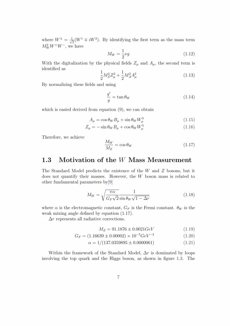
1.3 Motivation of the W Mass Measurement
The Standard Model predicts the existence of the W and Z bosons, but itdoes not quantify their masses. However, the W boson mass is related toother fundamental parameters by[9]
MW =
√πα
GF
√2
1
sin θW
√1−∆r
(1.18)
where α is the electromagnetic constant, GF is the Fermi constant. θW is theweak mixing angle defined by equation (1.17).
∆r represents all radiative corrections.
MZ = 91.1876± 0.0021GeV (1.19)
GF = (1.16639± 0.00002)× 10−5GeV −2 (1.20)
α = 1/(137.0359895± 0.0000061) (1.21)
Within the framework of the Standard Model, ∆r is dominated by loopsinvolving the top quark and the Higgs boson, as shown in figure 1.3. The
7

contribution from the tb loop is substantial due to the large mass differencebetween the two quarks. It depends on the top quark mass as ∝ M2
t . Thecorrection from the Higgs loop is proportional to lnMH . So by measuring thetop quark mass and W boson mass, the Higgs boson mass can be constrainedwithin the Standard Model. Beyond the Standard Model, there are also someother corrections. For example, in the minimal supersymmetric extension ofthe Standard Model (MSSM), corrections from the squark loops (figure 1.4)can increase the predicted W mass by up to 250 MeV[10][11].
For equal contributions to the Higgs mass, it is required that the accuraciesof the measurements of the W boson and top quark masses be related by
∆MW ≈ 0.006 ·∆Mt. (1.22)
Currently, the top quark has been measured with an uncertainty of about 1.3GeV[12]. That means the W mass needs to be measured with an uncertaintyof 8 MeV to provide an equivalent constraint. However, the world average ofthe W mass uncertainty is so far 25 MeV. The W boson mass is the limitingfactor in constraining the Higgs boson mass. Figure 1.5[13] shows the Higgsmass as a function of the W mass and top quark mass.
1.4 Previous Measurements of MW
Continuous efforts have been made to measure the W boson mass by dif-ferent experiments[15][16] as listed in figure 1.6[13] ever since the W and Zbosons[17] were discovered at CERN by UA1 and UA2 in 1983 with a Wmass of 81 ± 5 GeV . From 1996 to 2000, the four experiments of LEP atCERN - ALEPH, DELPHI, l3 and OPAL measured the boson mass with e+e−
collisions at center-of-mass energies above the W pair production threshold,√s > 2MW . The combined result of the W boson mass from LEP is 80.376
± 0.033 GeV [13]. The measurements were performed using W pair hadronicdecays into four quark jets, leptonic decays into four leptons(two charged lep-tons + two neutrinos) or hadronic + leptonic decays. The advantage of theLEP experiments is mainly their insensitivity to the theoretical description ofthe proton or anti-proton content. The bottom part in figure 1.6 from NuTeV,LEP1/SLD, and LEP1/SLD/mt show the indirect constraints[13][14] whichare not included in the world average.
The Collider Detector at Fermilab(CDF) and DØ experiments at the Fer-milab Tevatron collider(proton and anti-proton at
√s = 1.8 TeV) measured
the W mass using data collected from 1992 to 1995 with an uncertainty below100 MeV. Since 2001, the upgraded CDF and DØ experiment have been taking
8
data at the upgraded Tevatron at center-of-mass energy√
s = 1.96 TeV. In2007, CDF published their result using 200 pb−1 data with the measured Wmass value 80.413 ± 0.0048 GeV.
In this thesis, a precision measurement of the W boson mass using DØdata collected from 2002 to 2006 will be presented.
9

Figure 1.1: The fundamental particles in the Standard Model
10

Figure 1.2: Proton and Neutron
Figure 1.3: One-loop top quark and Higgs corrections to the W boson mass.
Figure 1.4: One-loop squark corrections to the W boson mass.
11

80.3
80.4
80.5
150 175 200
mH [GeV]114 300 1000
mt [GeV]
mW
[G
eV]
68% CL
∆α
LEP1 and SLD
LEP2 and Tevatron (prel.)
March 2009
Figure 1.5: Higgs mass constraints as function of MW and Mtop. The greenband is prediction of the Higgs mass, with 160 GeV to 170 GeV recently ruledout by Tevatron(the white stipe) with 95% C.L. The blue contour correspondsto the 68% C.L.
12

W-Boson Mass [GeV]
mW [GeV]80 80.2 80.4 80.6
χ2/DoF: 1.2 / 1
TEVATRON 80.432 ± 0.039
LEP2 80.376 ± 0.033
Average 80.399 ± 0.025
NuTeV 80.136 ± 0.084
LEP1/SLD 80.363 ± 0.032
LEP1/SLD/mt 80.364 ± 0.020
March 2009
Figure 1.6: Previous measurements of MW
13

Chapter 2
Experimental Apparatus
2.1 The Fermilab Accelerator System
The proton-antiproton collision beams are provided by the Tevatron, whichis a circular particle accelerator at the Fermi National Accelerator Labora-tory(FNAL) in Batavia, Illinois, USA. It is still the highest energy particlecollider operating in the world. Protons and antiprotons are accelerated toenergies of 0.98 TeV every 396 ns at Tevatron. Details about the acceleratorare documented in reference [15][18][19].
The accelerator is composed of a number of different accelerator systems:the Pre-accelerator, Linac, and Booster (collectively known as the ProtonSource), Main Injector, Tevatron, Debuncher and Accumulator (These lasttwo machines are referred to as the Antiproton Source). Figure 2.1 is theoverview of the accelerator at Fermilab.
2.1.1 Preac, Linac and Booster
The Pre-accelerator(Preacc), is a Cockcroft-Walton accelerator. It providesthe source of the negatively charged H− ions accelerated by the linear acceler-ator. The H− gas is accelerated through a column from the charged dome(-750kV) to the grounded wall to acquire an energy of 750 keV.
The Linear Accelerator(Linac) accelerates the H− ions with an energy of750 KeV to an energy of 400 MeV. It has two main sections, the low energydrift tube Linac(DTL) and the high energy side coupled cavity Linac(SCL).DTL focuses the beam by means of quadrupole magnets located inside thedrift tubes.The beam traveling through the SCL is focused by quadrupolesplaced between the accelerating modules.
The Booster is the first circular accelerator, or synchrotron, in the chain
14

MAIN INJECTOR (MI)
LINAC
BOOSTER
120 GeV p8 GeVINJ
p ABORT
TEVATRON
p ABORT
SWITCHYARD
RF150 GeV p INJ150 GeV p INJ
p SOURCE:DEBUNCHER &ACCUMULATOR
_
p_
pF0
A0
CDF DETECTOR& LOW BETA
E0 C0
DO DETECTOR& LOW BETA
p (1 TeV)
p (1 TeV)_
TeV EXTRACTIONCOLLIDER ABORTS
_
B0
D0
_
P1
A1
P8
P3
P2
TEVATRON EXTRACTIONfor FIXED TARGET EXPERIMENTS
& RECYCLER
PRE-ACC
Figure 2.1: Accelerator Overview
of accelerators. It takes the 400 MeV negative hydrogen ions from the Linacand strips the electrons off, which leaves only the proton, and accelerates theprotons to 8 GeV. The Booster can accelerate beam once every 66 milliseconds(15 Hz).
2.1.2 Main Injector
The Main Injector (MI) is a circular synchrotron seven times the circumferenceof the Booster and slightly more than half the circumference of the Tevatron.It consists of 6 sections, labeled MI-10 through MI-60. The MI can accelerate8 GeV protons from the Booster to either 120 GeV or 150 GeV, dependingon their destination. The Main Injector can provide beam to a number ofdifferent places at a number of different energies. It can operate in differentmodes:
• Pbar Production: It produces Pbars, to put in a stack in the accumula-
15

tor.
• Shot Setup: This mode relates to the act of extracting a bunch of antipro-tons from the Antiproton Source and inserting them into the Tevatron.
• The NuMI experiment: The MI sends protons to the NuMI target toproduce neutrinos.
• Other modes
2.1.3 Tevatron
The Tevatron is the largest of the Fermilab accelerators, with a circumferenceof approximately 4 miles. The Tevatron can accept both protons and antipro-tons from Main Injector and accelerate them from 150 GeV to 980 GeV. InCollider mode, the Tevatron can store beam for hours at a time. Because theTevatron is a primarily storage ring, the length of time between accelerationcycles is widely variable. The magnets used in the Tevatron use wire madefrom superconducting niobium/titanium alloy that needs to be kept extremelycold (∼4 K) by liquid helim to remain a superconductor.
2.1.4 Antiproton Source
The Antiproton Source is composed of the following parts.
• Target: During stacking, 120 GeV protons coming from the MI are di-rected to strike a nickel target. 8 GeV antiprotons are collected by usingmagnets out of all sorts of secondary particles produced by the collision.These antiprotons are directed down into the Debuncher.
• Debuncher: It can accept 8 GeV protons from Main Injector for beamstudies, and 8 GeV antiprotons from the target station. Its primarypurpose is to efficiently capture the high momentum spread antiprotonscoming off of the target.
• Accumulator: It is the second synchrotron of the antiproton source andused to store the antiprotons.
2.2 Run IIa DØ Detector
The DØ detector for Run IIa was constructed to study proton-antiprotoncollisions at a center of mass energy
√s = 1.96 TeV. It is a multipurpose
collider detector, optimized to follow three general goals[20]:
16

• Excellent identification and measurement of electrons and muons.
• Good measurement of high pT quark jets through finely segmented calorime-try with good energy resolution.
• A well-controlled measurement of missing transverse energy to charac-terize the presence of neutrinos and other non-interacting particles.
Figure 2.2 is the overview of the DØ detector. A Cartesian coordinatesystem is used with the z axis defined by the direction of the proton beam,the x axis pointing radially out of the Tevatron ring, and the y axis pointingup[25][26]. In proton-antiproton collisions the center of mass frame of thecolliding partons is approximately at rest in the plane transverse to the beamdirection, but the motion along the beam direction of some secondaries cannot be determined because of the beam pipe. Therefore the plane transverse tothe beam direction is of special importance, and sometimes we work with two-dimensional vectors defined in the x-y plane. We use rapidity y = +1
2ln(E+pz
E−pz)
to define the direction of a particle relative to the beam direction. The rapidityis additive under Lorentz boosts in the beam direction. For a particle withenergy much greater than its mass, the pseudorapidity η = −ln tan(θ/2) isused as a good approximation of rapidity. The DØ detector covers a rangeof |η| < 4.2. Its most important components are the central tracking system,uranium/liquid-argon calorimeter and muon system. In the next sections forthe subdetectors, we will follow the discussions in reference [26][28].
2.2.1 Central Tracking System
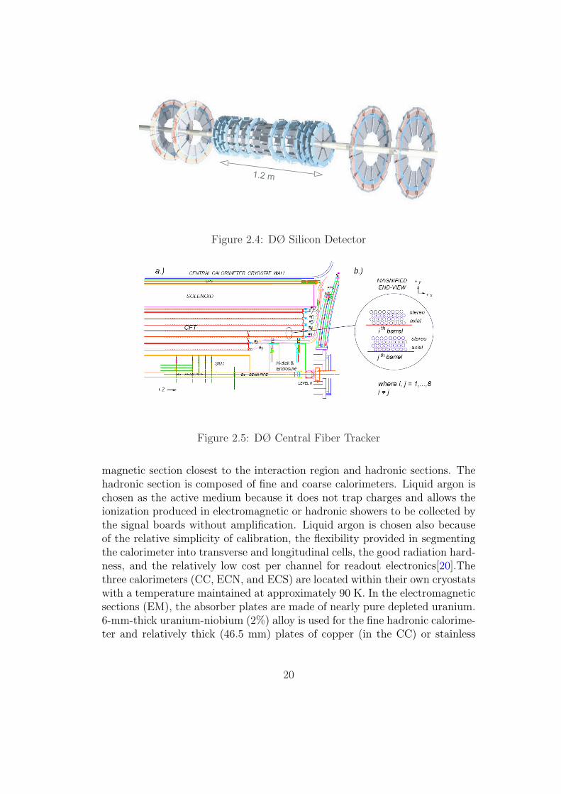
The central tracking system is composed of the silicon microstrip tracker(SMT)and the central fiber tracker (CFT) surrounded by a solenoidal magnet asshown in figure 2.3. They were designed for the excellent tracking measurementin the central region for studies of top quark, electroweak, and b physics andto search for new phenomena, including the Higgs boson.Silicon Microstrip Tracker(SMT)The SMT[21] is built to perform the tracking and vertexing over nearly thefull coverage of the calorimeter and muon systems. A overview of the SMTis shown in figure 2.4. It has six barrels in the central region, in each ofwhich there are four silicon readout layers. Each barrel is capped at high |z|with an F-disk, which consists of twelve double-sided wedge detectors. Thebarrel detectors primarily measure the position in the r-φ plane and the diskdetectors measure the position in both r-z and r-φ planes. There are anotherthree F-disks on each side of the forward region. H-disks are sitting in the
17

Calorimeter
Shielding
Toroid
Muon Chambers
Muon Scintillators
η = 0 η = 1
η = 2
[m]
η = 3
–10 –5 0 5 10
–5
0
5
Figure 2.2: DØ Detector
far forward regions to measure tracks at high |η|. The SMT has 912 readoutmodules, with 792,576 channels.Central Fiber Tracker(CFT)Outside the SMT is the Central fiber tracker(CFT)[22] as shown in figure2.5. The CFT is made up of scintillating fibers mounted on eight concentricsupport cylinders, at radii from 20 to 52 cm. It covers a range of η ≤ 1.7. Pho-tons produced by an ionizing particle are detected by a Visible Light PhotonCounter (VLPC) that converts the photons into an electrical pulse. The CFThas 76,800 scintillating fibers grouped into doublet layers and can measurethe position with a resolution on the order of 100 µm, corresponding to a φresolution of 2× 10⁻⁴ radians.
2.2.2 Solenoid and Preshower
The 2T magnetic field in the central tracking system is provided by the su-perconducting solenoidal magnet. The magnet was designed to optimize themomentum resolution and tracking pattern recognition within the constraints
18

Solenoid
Preshower
Fiber Tracker
Silicon Tracker
η = 0 η = 1
η = 2
[m]
η = 3
–0.5 0.0–1.5 0.5 1.0 1.5–1.0
–0.5
0.0
0.5
Figure 2.3: DØ Tracking System
imposed by the DØ calorimeter.The preshower[23][24] detectors are added to help identify electrons and
reject background during both triggering and offline reconstruction by en-hancing the spatial matching between tracks and calorimeter showers. Thecentral preshower detector covers the region |η| < 1.3 and the two forwardpreshower detectors cover 1.5 < |η| < 2.5. The preshower detectors are notused in the W mass measurement due to the electronics saturation from thehigh luminosity during the RunII data taking.
2.2.3 Calorimeter
To the W mass measurement at DØ the most important subdetector is theuranium/liquid-argon sampling calorimeter(figure 2.6). It is well suited toidentify electrons, photons and jets and also measure their energies. A signif-icant improvement to the detectors performance resulted from the removal ofthe old Main Ring beam pipe from the calorimeters(compared to Run I). Re-moval of the Main Ring increased the livetime of the detector by approximately10%, depending on the trigger[26][27].
The calorimeter has one central calorimeter covering |η| < 1.1. The twoforward calorimeter cover 1.5 < |η| < 4.2, as shown in figure 2.7. Each of themis contained in its own cryostat and can be further categorized into an electro-
19
1.2 m
Figure 2.4: DØ Silicon Detector
Figure 2.5: DØ Central Fiber Tracker
magnetic section closest to the interaction region and hadronic sections. Thehadronic section is composed of fine and coarse calorimeters. Liquid argon ischosen as the active medium because it does not trap charges and allows theionization produced in electromagnetic or hadronic showers to be collected bythe signal boards without amplification. Liquid argon is chosen also becauseof the relative simplicity of calibration, the flexibility provided in segmentingthe calorimeter into transverse and longitudinal cells, the good radiation hard-ness, and the relatively low cost per channel for readout electronics[20].Thethree calorimeters (CC, ECN, and ECS) are located within their own cryostatswith a temperature maintained at approximately 90 K. In the electromagneticsections (EM), the absorber plates are made of nearly pure depleted uranium.6-mm-thick uranium-niobium (2%) alloy is used for the fine hadronic calorime-ter and relatively thick (46.5 mm) plates of copper (in the CC) or stainless
20

steel (EC) are used for the coarse hadronic modules .
DØ's LIQUID-ARGON / URANIUMCALORIMETER
1m
CENTRAL
CALORIMETER
END CALORIMETER
Outer Hadronic
(Coarse)
Middle Hadronic
(Fine & Coarse)
Inner Hadronic
(Fine & Coarse)
Electromagnetic
Coarse Hadronic
Fine Hadronic
Electromagnetic
Figure 2.6: DØ Uranium/Liquid-argon Calorimeter
The CC-EM section is composed of 32 azimuthal modules. The entirecalorimeter is divided into about 5000 pseudoprojective towers, each covering0.1×0.1 in η×φ. The EM section is segmented into four layers, 2, 2, 7, and 10radiation lengths thick respectively. The third layer, in which electromagneticshowers typically reach their maximum, is transversely segmented into cellscovering 0.05×0.05 in η × φ (figure 2.8). The hadronic section is segmentedinto four layers (CC) or five layers (EC). The entire calorimeter is 7 to 9nuclear interaction lengths thick. The signals from arrays of 2×2 calorimetertowers, covering 0.2×0.2 in η×φ, are added together electronically for the EMsection only and for all sections, and shaped with a fast rise time for use in thelevel 1 trigger. We refer to these arrays of 2×2 calorimeter towers as triggertowers[25].
Figure 2.9 is the schematic view of a typical calorimeter cell. The metalabsorber plates are grounded and the signal boards(G10 boards) with resistivesurfaces are placed at a high voltage of 2.0 kV. The electron drift time acrossthe 2.3 mm liquid argon gap is approximately 450 ns. The gap thickness waschosen to be large enough to observe minimum ionizing particle signals and toavoid fabrication difficulties. Particles traversing the gap generate an ionizedtrail of electrons and ions. The current, produced by the electrons drift inthe electric field, induces an image charge on a copper pad etched on the G10
21

Figure 2.7: DØ Uranium/Liquid-argon Calorimeter showing segmentation inη and depth
board under the resistive coat. The charge is then transferred to calorimeterreadout system.
Figure 2.10 shows a schematic of this data path. The signal from eachreadout cell is brought to a feed-through port on a 30 Ω coaxial cable. Thesignals are carried from the feed-through ports to the preamplifier inputs on115 Ω twist & flat cables. The image charge induced on the readout pads bythe charge collected on the resistive coat is integrated by the charge-sensitivepreamplifiers. The voltage pulses are transferred to the shaper and baselinesubtracter (BLS), where the preamplifier outputs are shaped, sampled beforeand after the bunch crossing, and the difference is stored on a sample & holdcircuit. The sample & hold outputs are then read out and digitized by theanalog to digital converters(ADCs) when a trigger is received.
It is very important to understand the calorimeter performance. The en-ergy resolution of the calorimeter can be written as equation 2.1.
σE
E=
√(N
E
)2
+
(S√E
)2
+ C2 (2.1)
where N , S and C are used in the noise, sampling, and constant terms,respectively. The noise term is from electronic noise summed over readoutchannels. The sampling term reflects statistical fluctuations such as intrinsic
22

Figure 2.8: Calorimeter channel layout in directions of depth and η
shower fluctuations, including dead material in front of the calorimeter andsampling fluctuations. The constant term accounts for contributions fromdetector non-uniformity and calibration uncertainty.
2.2.4 Muon System
The upgraded detector uses the original central muon system proportionaldrift tubes (PDTs) and toroidal magnets, central scintillation counters (somenew and some installed during Run I), and a completely new forward muonsystem. The new forward muon system extends muon detection from |η| ≤1.0 to |η| ≈ 2.0, using mini drift tubes (MDTs) instead of PDTs and includingtrigger scintillation counters and beam pipe shielding. A 1.8 T magnetic fieldis generated by a toroidal iron magnet in a second tracking system outside thecalorimeter to detect muons. Positions are measured by drift chambers. Inthe DØ W mass measurement, only the tracking system and calorimeter areused.
23

G10 InsulatorLiquid Argon
GapAbsorber Plate Pad Resistive Coat
Unit Cell
Figure 2.9: Liquid argon gap and signal board unit cell for the calorimeter
Figure 2.10: Simplified diagram of the calorimeter data flow path.
24

Chapter 3
Measurement Strategy
In the Z → ee events, the energy and directions of both electrons are measuredprecisely by the calorimeter(with fluctuations of order 4% for pT (e)=50 GeV)and the tracking system respectively[31]. However, in the W → eν events, theneutrino escapes detection and leaves behind substantial missing energy. If theW or Z has transverse momentum energy from the recoiling system, the recoilsystem spreads over a wide range in the detector. It consists of clusteredenergy as well as unclustered hadronic particles, which cannot be detected.Some of the recoil particles might go along the beam direction and carrysubstantial longitudinal momentum pZ . The initial longitudinal momentumsum is unknown, in addition. Therefore, the momentum component along thebeam direction of the neutrino cannot be inferred. The invariant W bosonmass is unable to be reconstructed. We then resort to the variables in thetransverse plane for the W mass information. A variable “Transverse Mass”is defined as
mT =√
2pT (e)pT (ν)(1− cos(φ(e)− φ(ν))), (3.1)
where φ(e) and φ(ν) are the azimuthal angles of the electron momentum and
the−→/ET direction, respectively.The variables mT and pT (e) are the two main observables in this measure-
ment. Figure 3.1 shows the different sensitivity of mT and pT (e). In the leftplot, mT is relatively insensitive to the transverse momentum of the W boson.However, since mT is calculated by using the /ET which is subject to the recoilresolution, mT is sensitive to the detector effects. In the right hand plot, pT (e)is sensitive to the pT (W ), which requires a precise calculation of the produc-tion dynamics of the W boson. Thanks to the better resolution in measuringthe energy of electrons than neutrinos, pT (e) is barely sensitive to the detectoreffects. The variables mT and pT (e) thus provide us with two complementarydistributions. The pT (ν) is sensitive to both the detector and boson kinematic
25

effects, which can serve as a cross-check.
3.1 Fast Simulation
Due to the fact that the three distributions are sculpted by the complex de-tector acceptance and resolution effects, their shapes cannot be calculatedanalytically. We build a fast parameterized Monte Carlo(fast MC) to simulatethe detector and offline selection effects, which smears the events generated bycertain event generators. A group of mass templates(distributions predictedby the fast MC) of the prediction of the mT , pT (e) and /ET are generated byvarying the input W mass. We compare the templates with the correspond-ing distribution obtained from collider data to extract the W mass value withwhich the best agreement is achieved. High statistics(∼ 108 events) is requiredto characterize the different systematic uncertainties with sufficient precision.It is unpractical to simulate the same number of events by using the detailedsimulation based on GEANT(full MC), which uses physics principles to modelthe interaction between particles and detector material. It is also not feasibleto tune the full MC to simulate the real detector to the precision needed forthe W mass measurement. Due to the above reasons, the fast MC is a goodchoice, with which we can quickly simulate the necessary events and easilymake modifications to find the best match with the data during the modeltuning. In tuning the parameters used in the fast MC, Z → ee samples areextensively used to calibrate the detector response to the energy of electronsand the recoil system, find the selection efficiency, etc. The electron energyresponse is calibrated by forcing the simulated invariant mass of the two Zelectrons to be consistent with the world average Z mass. Since the mT andZ mass are equally sensitive to the electron energy response, we are essentiallymeasuring the ratio of W and Z masses.
3.2 Fitting Method
In extracting the W mass by fitting the mass templates with the distributionsfrom collider data, a binned negative log likelihood technique is used. Thelikelihood is calculated as the product of the Poisson probability for each bin,with ni observed events and mi expected events:
L =N∏
i=1
e−mimnii
ni!. (3.2)
26

By taking the logarithm on both sides, we get
lnL =N∑
i=1
(ni ln mi −mi) , (3.3)
where the ln(ni!) term is a constant so we can ignore it in performing thevariations.
Using Minuit [30] we find the mass that minimizes − lnL and the ±1σvalues that increase − lnL by 0.5. The fits are performed separately for eachof the mT , pT (e) and /ET distributions.
3.3 Blinding Technique
The W boson mass has been estimated to be a world average of 80.398 ±0.025 GeV by combining results from many experiments. To avoid the influ-ence on the analyzers from the world average W mass value, it is importantto not let the analyzers know the true measured W mass value during theanalysis. In light of that, we performed a ”blind analysis” in the Run II Wmass measurement[32]. The central value of the measured W mass was hiddenfrom the analyzers and the rest of the collaboration until the agreement be-tween the data and the fast MC reached sufficient quality and the analysis hasreceived preliminary approval from the Editorial Board and the collaboration.An unknown offset in the range [-2 GeV, 2 GeV] was added to the measured Wmass. To compare the measured W mass from the three variables(mT , pT (e)and /ET ), the same offset is applied to them.
27

mT (GeV)
dN/d
mT
55 60 65 70 75 80 85 90 95
pT(e) (GeV)
dN/d
p T(e
)
30 35 40 45 50
Figure 3.1: Top: mT distribution; Bottom: pT (e) distribution(Black: genera-tor level with zero pT (W ); Red: generator level with non-zero pT (W ); Yellow:Detector effect added)
28

Chapter 4
Data Samples
Three sets of data samples are used with an integrated luminosity of 1.046 fb−1
collected from 2002 to 2006 in Run II(figure 4.1): 2EM sample for selectingZ → ee events, EM+/ET sample for selecting W → eν events and EM+Jetsample for selecting 2Jet events for QCD background study. The averageinstantaneous luminosity during this period was 41 ×1030 cm−1s−1 with anaverage of 1.2 interactions per bunch crossing.
Figure 4.1: DØ RunII instantaneous luminosity vs time
29

The following requirements were used to select these three samples.
• EM+/ET :1 EM with pT > 20 GeV, | ηdet |< 1.2, fEM > 0.9 and raw /ET > 20 GeV
• 2 EM:2EM with pT > 20 GeV, fEM > 0.9 and fiso < 0.21
• EM+Jet:1 EM with pT > 20 GeV, | ηdet |< 1.2, fEM > 0.9, fiso < 0.2,1 Jet with pT > 20 GeV, | ηdet |< 0.8 or 1.5 <| ηdet |< 2.5,0.05<emfrac<0.95, chfrac<0.4, hotcellratio< 10 and n90>10
Here, emfrac is the fraction energy deposited in the electromagnetic section ofthe calorimeter, chfrac is the fraction of the jet energy deposited in the coarsehadronic section of the calorimeter, hotcellratio is the ratio of the highest tothe next-to-highest transverse energy cell in the calorimeter, n90 is the numberof towers containing 90% of the jet energy[33].
The sam dataset definitions for the selected samples are:
• EM+/ET :WMASSskim3-EMMET-WMRESK p17.09.03-ROOT-wm1,WMASSskim3-EMMET-WMRESK p17.09.06-ROOT-wm1,WMASSskim3-EMMET-WMRESK p17.09.06b-ROOT-wm1
• 2EM:WMASSskim3-2EM-WMRESK p17.09.03-ROOT-wm1,WMASSskim3-2EM-WMRESK p17.09.06-ROOT-wm1,WMASSskim3-2EM-WMRESK p17.09.06b-ROOT-wm1
• EM+Jet:tmb WMASSskim3-EMJET-WMRESK p17.09.03,tmb WMASSskim3-EMJET-WMRESK p17.09.06,tmb WMASSskim3-EMJET-WMRESK p17.09.06b.
4.1 Triggers
During the period of this data collecting, 4 trigger lists were used in the or-der of time: v8-11, v12, v13 and v14. Each trigger list is a combination ofthree trigger levels: L1/L2/L3. The first level(L1) is composed of hardwaretrigger elements which generate an acceptance rate of 2 kHz. On the second
1fEM and fiso are defined in section 4.2.2.
30
level(L2), a trigger decision is made based on individual objects as well as ob-ject correlations with an acceptance rate of about 1 kHz. The third level(L3)uses sophisticated algorithms on the candidate events sent by L1 and L2 andreduces the rate to approximately 50 Hz.
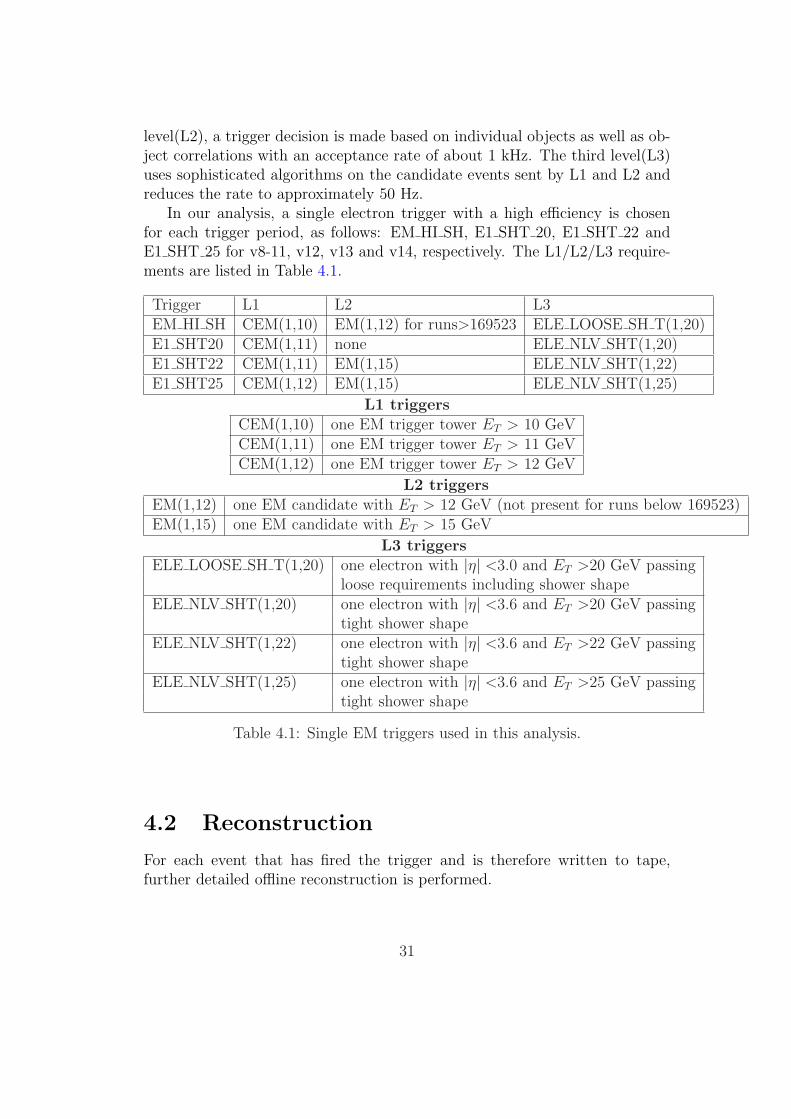
In our analysis, a single electron trigger with a high efficiency is chosenfor each trigger period, as follows: EM HI SH, E1 SHT 20, E1 SHT 22 andE1 SHT 25 for v8-11, v12, v13 and v14, respectively. The L1/L2/L3 require-ments are listed in Table 4.1.
Trigger L1 L2 L3EM HI SH CEM(1,10) EM(1,12) for runs>169523 ELE LOOSE SH T(1,20)E1 SHT20 CEM(1,11) none ELE NLV SHT(1,20)E1 SHT22 CEM(1,11) EM(1,15) ELE NLV SHT(1,22)E1 SHT25 CEM(1,12) EM(1,15) ELE NLV SHT(1,25)
L1 triggersCEM(1,10) one EM trigger tower ET > 10 GeVCEM(1,11) one EM trigger tower ET > 11 GeVCEM(1,12) one EM trigger tower ET > 12 GeV
L2 triggersEM(1,12) one EM candidate with ET > 12 GeV (not present for runs below 169523)EM(1,15) one EM candidate with ET > 15 GeV
L3 triggersELE LOOSE SH T(1,20) one electron with |η| <3.0 and ET >20 GeV passing
loose requirements including shower shapeELE NLV SHT(1,20) one electron with |η| <3.6 and ET >20 GeV passing
tight shower shapeELE NLV SHT(1,22) one electron with |η| <3.6 and ET >22 GeV passing
tight shower shapeELE NLV SHT(1,25) one electron with |η| <3.6 and ET >25 GeV passing
tight shower shape
Table 4.1: Single EM triggers used in this analysis.
4.2 Reconstruction
For each event that has fired the trigger and is therefore written to tape,further detailed offline reconstruction is performed.
31

4.2.1 Track and Vertex
Charged particles leave curved trajectories under the action of the magneticfield in the central tracking system. The transverse momentum(pT ) of the trackis measured from the curvature of the track. The track path is reconstructedby using the hits from the SMT and CFT. Since Run I, the road-followingalgorithm has been used in finding tracks[34]. In Run II, a Kalman filter[35]is implemented in addition. Global track candidates are constructed after thetrack segments that are produced for each layer are matched between layers.A χ2 calculated for the fit between a track and the nearby hits is used todetermine whether to accept the track or not.
The primary vertex tells us the parton collision location of incoming par-ticles, which is associated with a lot of tracks. Precise reconstruction of theprimary vertex is crucial in calculating the transverse momentum of the recoilsystem. Long-lived particles such as B, KS or D bring secondary vertices. Theprimary vertex candidate is selected by requiring global tracks with at leastSMT hit. Then a vertex position is extracted by fitting these tracks until thefit result converges. More details about the primary and secondary vertexreconstruction can be found in [36].
4.2.2 Electron
An electron is identified as a cluster of adjacent calorimeter cells. Its energy iscalculated as the sum of the energies in all the EM and FH1 cells in a cone ofsize R =
√(∆η)2 + (∆φ)2 = 0.2, centered on the tower with the highest frac-
tion of the electron energy. If the electron is associated with a track detectedin the central tracking system, the track direction will be taken as the electrondirection.
θ(e) = θtrack
φ(e) = φtrack
Otherwise, the electron direction is calculated using the calorimeter showercentroid position and the primary vertex position. For the final Z and Wsamples, the track match is always required to select electrons, so the electrondirection is using the track direction. When estimating the track match effi-ciency, we do use electrons without the track match where the electron clusterdirection is used.
Electromagnetic clusters found by the reconstruction(EMReco) are requiredto satisfy ET > 1.5 GeV, fEM > 0.9 and fiso < 0.15. ET is the transverseenergy of the EM cluster deposited in the calorimeter. fEM is the EM cluster
32

energy fraction in the EM part of the calorimeter
fEM =EEM
EEM + EHad
, (4.1)
where EEM and EHad are the energy measured in the EM and Hadronic partof the calorimeter in a cone of radius R =
√∆η2 + ∆φ2 = 0.2 , respectively.
fiso is the isolation with the definition
fiso =ETot(R < 0.4)− EEM(R < 0.2)
EEM(R < 0.2), (4.2)
where ETot(R < 0.4) is the total energy in a cone of radius R = 0.4 aroundthe direction of the cluster, summed over the entire depth of the calorimeterand EEM(R < 0.2) is the energy in a cone of R = 0.2, summed over the EMlayers only. Figure 4.2 gives a straightforward view of the isolation definition.
Figure 4.2: Isolation definition
The variables fEM and fiso provide powerful rejection to the hadronic jetsthat tend to deposit most of their energies in the hadronic calorimeter and arecomposed of nonisolated particles.
The shower shape of an electron is defined using a covariance matrix tech-nique for electron candidates central calorimeter(CC). To achieve the best
33

discrimination against hadronic jets, both longitudinal and transverse showershape variables are used, along with the correlations between energy depositsin the calorimeter cells. The inverse of this covariance matrix is called theH-matrix. The H-matrix(7)(HMx7) for central calorimeter is built up with aset of seven variables[37]:
• EM fraction in EM calorimeter layers EM1
• EM fraction in EM calorimeter layers EM2
• EM fraction in EM calorimeter layers EM3
• EM fraction in EM calorimeter layers EM4
• transverse shower width in the φ direction
• log10(Energy)
• vertex z position
HMx7 is optimized by using full MC to determine a χ2 value. Typicallywe require HMx7 < 12 to select electrons. For electrons in the End Calorime-ter(EC), HMx8 is used in stead, which is built up with the above seven vari-ables and the following variable:
• transverse shower width in the z direction
To further reject the hadronic jets background, a spatial track match vari-able is defined using both the track and calorimeter information.
χ2 = (∆z
σz
)2 + (∆φ
σφ
)2, (4.3)
where ∆z and ∆φ are the differences between the track position and the EMcluster position in the calorimeter. The σz and σφ are the tracking resolutionin z and φ, respectively. For a good match, the spatial track matching χ2
probability P (χ2) > 0.01.In the DØ W mass measurement, we also require each track to have at
least one hit in the SMT and the track pT measured by the tracking system isgreater than 10 GeV.
34

4.2.3 /ET
Since the neutrino escapes the detector without being detected, the rest of theevent is the hadronic recoil system, which mainly comes from the initial gluonradiation and hadronization, along with the spectator partons interactions, ad-ditional proton-antiproton interactions, electronic noise, etc. Since transversemomenta of all the particles except the neutrino in each event are measuredby the detector, we infer the neutrino transverse momentum by balancing thetransverse momentum from other particles in the event:
/ETraw = −
∑i
Ei sin θi
(cos φi
sin φi
)= −
∑i
EiT , (4.4)
where the sum goes over all the calorimeter(central and forward) read out cellsexcept cells in the coarse hadronic calorimeter. Ei are the cell energies, andφi and θi are the azimuth and colatitude of center of cell i with respect tothe primary vertex. After we have the raw missing transverse energy, we thenapply electron energy corrections on the selected EM cluster(s) from W (Z)decay to get the corrected missing transverse energy /ET . The IntercryostatDetector(ICD) (1.1 < |ηdet| < 1.4) is not included due to an unsatisfactorycalibration. As previously mentioned, the primary vertex is crucial in calcu-lating the /ET . In recognition of that, we compare the z-component of theelectron(s) vertex with that of the event primary vertex. If they are consistentwithin 2 cm, we will still use the event primary vertex, otherwise we will takethe electron(s) vertex as the primary vertex to calculate the /ET .
The scalar ET (SET) is defined as
SET =∑
i
Eisinθi (4.5)
in which cells in electron clusters are excluded from the sum. The sum goesthrough the whole calorimeter(both CC and EC) excluding the ICD and thecoarse hadronic calorimeter.
In this analysis the raw energy is used for the recoil since we mostly studyevents with low boson transverse momentum. In this situation the hadronicrecoil system is mainly composed of unclustered particles which spread widelyin the detector and therefore no jet energy scale is applied.
35

4.2.4 Recoil
The recoil uT for W/Z boson events can be defined from the /ET and theelectron(s) transverse momentum:
uT = −/ET −∑
e
peT =
∑i
EiT −
∑e
peT (4.6)
4.3 Offline Selection
The next step after the reconstruction is the offline selection.
• |Z|< 60 cm
Electron selection:
• EM ID=10,±11, fEM > 0.9, fiso < 0.15(EM=10 for an EM cluster without an associated track and ±11 withan associated track)
• pT > 25 GeV
• HMx7< 12 in CC and HMx8< 20 in EC
• In calorimeter fiducial region (in eta fiducial and in phi fiducial)
• Spatial track match
• Associated track must have at least one SMT hit and pT > 10 GeV
Z → ee requirements:
• At least one electron passes trigger requirements (L1/L2/L3)
• Both electrons have good matched track
• Electron |ηdet| < 1.05
• uT < 15 GeV
• 70 < Mee < 110 GeV
W → eν requirements:
• The electron must pass trigger requirements (L1/L2/L3)
• The electron must have a good matched track
36

• Electron |ηdet| < 1.05
• uT < 15 GeV
• 50 < MT < 200 GeV
After the offline selection we have 499,830 W → eν candidate events and18,725 Z → ee candidate events.
4.4 Energy Loss Correction
The electron energy is measured by the DØ uranium/liquid-argon samplingcalorimeter, where the electron largely develops its electromagnetic shower.However, before reaching the calorimeter, the electron has to travel throughdead material(figure 4.3) such as the inner detector, solenoidal magnet, inter-cryostat detector, etc. This uninstrumented material(for calorimetry) is calledthe “dead” material and is in cylindrical shape around the beam line with athickness of about 3.7 radiation lengths(X0). The electron loses some of itsenergy in this material. The lost energy is estimated by using the standardDØ full MC single electron events. In the full MC, the interaction betweenthe electron and the material in the detector is simulated. The concern is: isthe amount of material in front of the calorimeter simulated correctly in thefull MC or not? A detailed study did tell us the amount of the dead materialis underestimated in the full MC compared to the data.
To best estimate how much material is missing in the full MC, we needa good way to test the performance of simulations, and in particular aspectsrelated to the material model, for example, by checking the well-known invari-ant mass and the width of the Z boson. Another class of observables [38] aresuggested to exploit the longitudinal segmentation of the calorimeter readout.In our case this means looking at the “EM fractions”, i.e. at the fraction ofthe measured electron energy deposited in each one of the longitudinal layers(EM1, EM2, EM3 and EM4; and in principle also FH1 but the deposits in FH1are typically negligibly small) for electrons from a well-characterized source.Figure 4.4 shows the average electron shower profile with two different anglesof incidence. If we increase the amount of the dead material, the calorimeterwill be “shifted” deeper into the shower. The second and third EM layers aresitting right on the edge of the shower peak, so the electron energy fractiondeposited in these three layers is very sensitive to the amount of the deadmaterial.
The two plots in figure 4.4 also demonstrate the amount of deal materialthat an electron travels through strongly depends on the electron incidence
37

Figure 4.3: Overview of the uninstrumented (from the point of view ofcalorimetry) material in front of the Central Calorimeter. This drawing hasbeen reproduced from Ref. [26] and shows a cross-sectional view of the centraltracking system and in the x − z plane. Also shown are the locations of thesolenoid, the preshower detectors, luminosity monitor and the calorimeters.
angle. So instead of only looking at the observables averaged over our entire Zsample, we split the sample in a clever way, based on the electron energy andphysics η (which is related to angle of incidence on the dead material). Wedefine five bins in the absolute value of electron physics η (|ηphys|) which is usedas a measure of the angle of incidence on the dead material. The exact defini-tion is given in table 4.2. We classify these events into 15 distinct categoriesaccording to the |ηphys| bin of each of the two electrons without distinguishingthe leading and the subleading electron to avoid having to worry about thecalorimeter energy resolution. Therefore we have 15 unique categories, whichare defined in table 4.3.
To compare the different EM fractions for electrons from Z → ee be-
38
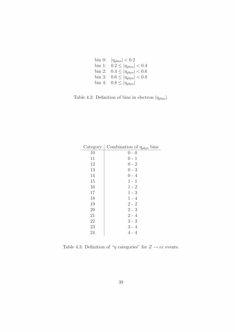
bin 0: |ηphys| < 0.2bin 1: 0.2 ≤ |ηphys| < 0.4bin 2: 0.4 ≤ |ηphys| < 0.6bin 3: 0.6 ≤ |ηphys| < 0.8bin 4: 0.8 ≤ |ηphys|
Table 4.2: Definition of bins in electron |ηphys|.
Category Combination of ηphys bins10 0 - 011 0 - 112 0 - 213 0 - 314 0 - 415 1 - 116 1 - 217 1 - 318 1 - 419 2 - 220 2 - 321 2 - 422 3 - 323 3 - 424 4 - 4
Table 4.3: Definition of “η categories” for Z → ee events.
39

tween data and the simulation, we make use of a combination of slow2 firstprinciples calculations and parametrized Monte Carlo. Based on the singleelectron events from the detailed simulation, we construct a parameterisationof the mean EM fractions and fluctuations as a function of true electron energyand ηphys. The single electrons are produced at different values of energy andηphys and span the entire region of the energy/ηphys plane that is relevant forZ → ee.
Figure 4.5 shows the data/MC comparison of the EM fractions of cate-gories 10 and 23 respectively, in which there is this clear discrepancy betweenthe data and simulation. The less energy in the first EM layer and more en-ergy in the third EM layer from the simulation than from the data means,the electron shower is developing a littler later in the simulation than in thedata, which also proves the underestimation of the dead material in the sim-ulation. Figure 4.6 shows the means of the EM fractions for all EM layersand for all categories; separately for data and the simulation. We plot thedata/simulation ratio for each of the mean EM fractions in figure 4.7. Al-though the data/MC disagreement(the ratio deviation from unity)that we seein figure 4.7 is not caused alone by the missing dead material(for example,the missing layer-intercalibration), it certainly is larger than what one wouldexpect.
Now we need to add some additional uninstrumented material to the de-tector model and we chose a relatively low-Z material, namely copper, andplace it inside the solenoid. More precisely, the shape of this chunk of copperis cylindrical, it has the same axis of rotational symmetry as the solenoid, andit extends over the whole length in z of the solenoid. The shape of the missingmaterial is driven by the observation that the material in front of the centralcalorimeter all have a geometry that is close to cylindrical. We use the detailedfirst principles simulation to simulate single electrons with different amount ofmissing material added. Again, we build a parametrized model of the meanEM fractions and the fluctuations around the average. We take the numberof radiation lengths(nX0) of the missing material as the free parameter.
As shown in figure 4.7, we fit each of the data/MC ratios with a flat lineand sum the fitted χ2 from the three fits. Due to the small energy deposit inEM4, we do not include EM4 in our fits. The number of degrees of freedomfor the combined χ2 is 3∗15−3−1 = 41. The minimization of the χ2 in the fitis shown in Fig. 4.8. The result of the minimization and the fit results of theper-layer constants for the optimal value of nX0 are summarized in Tab. 4.4.
2Here, “slow” mainly means we used a smaller step size than in the standard full MCwhen simulating the interaction between an electron or photon and the detector material.So more time is taken to generate full MC events.
40

Additional material: nX0 = 0.1633± 0.0095
Per-layer constants: c(EM1) = 1.0064± 0.0013c(EM2) = 1.0001± 0.0007c(EM3) = 0.9833± 0.0008c(EM4) ' 1.05
Table 4.4: Summary of the results of the adjustment of nX0.
As a cross-check, we repeat the fit for nX0, separately for each of the threelayers. The results are summarized in figure 4.9. Good agreement is foundbetween the results from each of the individual layers.
After adding the missing material into the full MC, we rederive the E-loss corrections and energy resolution function for this measurement and weinterpret the small residual deviations from unity in the per-layer factors aslayer-intercalibration gain factors that we use to correct the data. Figure4.10 is an equivalent of Figure 4.5, except that the optimal value of nX0 hasbeen used and that the layer-intercalibration has been applied. Figure 4.10is showing we have achieved a lot better agreement between the data andsimulation after we add the missing material.
41
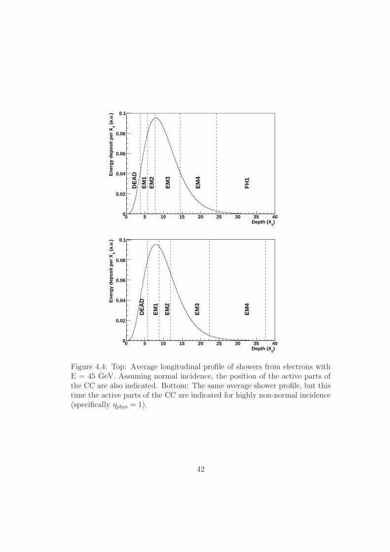
)0
Depth (X0 5 10 15 20 25 30 35 40
(a.
u.)
0E
ner
gy
dep
osi
t p
er X
0
0.02
0.04
0.06
0.08
0.1
DE
AD
EM
1E
M2
EM
3
EM
4
FH
1
)0
Depth (X0 5 10 15 20 25 30 35 40
(a.
u.)
0E
ner
gy
dep
osi
t p
er X
0
0.02
0.04
0.06
0.08
0.1
DE
AD
EM
1
EM
2
EM
3
EM
4
Figure 4.4: Top: Average longitudinal profile of showers from electrons withE = 45 GeV. Assuming normal incidence, the position of the active parts ofthe CC are also indicated. Bottom: The same average shower profile, but thistime the active parts of the CC are indicated for highly non-normal incidence(specifically ηphys = 1).
42

EMF10 0.1 0.2 0.3 0.4 0.5 0.6 0.7 0.8 0.9 1
0
50
100
150
200
250
300
ndof = 19 = 87.322χ
TOYEemf_1_10
EMF20 0.1 0.2 0.3 0.4 0.5 0.6 0.7 0.8 0.9 1
0
100
200
300
400
500
600
700
800
data
detailed response⊗ fast simulation
ndof = 6 = 29.082χ
TOYEemf_2_10
EMF30 0.1 0.2 0.3 0.4 0.5 0.6 0.7 0.8 0.9 1
0
50
100
150
200
250
300
350
ndof = 16 = 168.352χ
TOYEemf_3_10
EMF40 0.1 0.2 0.3 0.4 0.5 0.6 0.7 0.8 0.9 1
0
100
200
300
400
500
ndof = 12 = 4.482χ
TOYEemf_4_10
Figure 4.5: Comparison of EM fractions for electrons from Z → ee events incategory 10 in data and simulation. The four individual plots show the energyfraction in each of the four EM layers. The detailed response simulation usesthe default accounting of dead material.
43

Category10 12 14 16 18 20 22 24
EM
Fx
0
0.1
0.2
0.3
0.4
0.5
0.6EMF1, data
EMF2, data
EMF3, data
EMF4, data
EMFx, simulation
EMF per category
Figure 4.6: Summary of the means of the EM fraction distributions in Z → eeevents for each of the four EM layers and each of the 15 η categories; separatelyfor data and simulation.
44

Category10 12 14 16 18 20 22 24
MC
/ <E
MF
>d
ata
<EM
F>
0.85
0.9
0.95
1
1.05
1.1
1.15
EMF1
EMF2
EMF3
EMF4
EMF per category (data/MC)
Figure 4.7: Summary of the data/simulation ratios for the means of theEM fraction distributions in Z → ee events for each of the four EM layersand each of the 15 η categories. Each of the three horizontal lines indicatesthe result of a fit of a common constant to the the 15 data points from agiven EM layer. The fit was performed for EM1, EM2 and EM3. EM4 is notincluded because of the smallness of the energy deposits in it, especially atnon-normal incidence.
45

number of additional radiation lengths0.13 0.14 0.15 0.16 0.17 0.18 0.19
2 χ
38
40
42
44
46
48
ndof = 41 = 40.032χ
e e→ from longitudinal shower profiles in Z 0Fit for nX
Figure 4.8: Fit for nX0, the amount of uninstrumented material (in radiationlegths) missing from the nominal material map in the detailed simulation ofthe DØ detector. The five stars indicate the value of the combined χ2 forEM1-EM3, evaluated for five values of nX0. A parabola is fit through thesepoints in order to determine the minimum of the combined χ2. Also shownin the figure are the value of the combined χ2 at its minimum as well as theone-sigma variations of nX0.
46

0nX
0.05 0.1 0.15 0.2 0.25 0.3
EM1 0.0162±0.1648
EM2 0.0158±0.1705
EM3 0.0175±0.1528
Combined 0.0095±0.1633
Figure 4.9: Stability check: results of the fit for nX0, performed separately foreach of the three layers (EM1, EM2 and EM3). The result of the combined fitis also shown for comparison.
47

EMF10 0.1 0.2 0.3 0.4 0.5 0.6 0.7 0.8 0.9 1
0
50
100
150
200
250
ndof = 19 = 20.232χ
TOYEemf_1_10
EMF20 0.1 0.2 0.3 0.4 0.5 0.6 0.7 0.8 0.9 1
0
100
200
300
400
500
600
700
800data
detailed response⊗ fast simulation
ndof = 6 = 11.592χ
TOYEemf_2_10
EMF30 0.1 0.2 0.3 0.4 0.5 0.6 0.7 0.8 0.9 1
0
50
100
150
200
250
300
350
ndof = 16 = 18.772χ
TOYEemf_3_10
EMF40 0.1 0.2 0.3 0.4 0.5 0.6 0.7 0.8 0.9 1
0
50
100
150
200
250
300
350
400
450
ndof = 12 = 13.422χ
TOYEemf_4_10
Figure 4.10: Comparison of EM fractions for electrons from Z → ee eventsin category 10 in data and simulation. The simulation used here includesnX0 = 0.1633 radiation lengths of extra uninstrumented material in front ofthe CC calorimeter. The four individual plots show the energy fraction in eachof the four EM layers.
48

Chapter 5
Event Generation
The first step of the fast simulation is the event generation. Here the conciseintroduction will follow references [39] [40] [28].
5.1 Boson Production and Decay
At the Tevatron pp colliders large numbers of W± and Z0 bosons are produced,which are important to measure electroweak parameters, probe the internalstructure of nucleons, and monitor the collider luminosity. Any deviations ofthe observation from the theoretical prediction may imply new gauge inter-actions, supersymmetry, particle compositeness, or extra spatial dimensions.Understanding the boson production will also be crucial to the new physicssearches since the Standard Model W± and Z0 processes are the major irre-ducible backgrounds to these searches. At hadron colliders, the massive elec-troweak bosons are produced predominantly via quark-antiquark annihilationand detected by the decay into a pair of leptons. Typical W or Z observablesare modified by QCD and electroweak radiation from the hadronic initial state;production, propagation, and decay of massive bosons; and electroweak radi-ation from the leptonic final state. Fig. 5.1 shows the lowest order diagramsfor Z and W+ boson production.
For a process (pp → V ) (V stands for either the W or the Z intermediatevector boson) in the proton-antiproton collisions at the hadron collider, theparton-level cross section σ can be calculated as a function of the quark mo-menta, and then interplays with the distribution of quark momenta inside theproton and the antiproton
σ =∑i,j
∫ ∫dx1dx2fi/p(x1, s)fj/p(x2, s)σij(s) (5.1)
49

u
u–
Z0
u
d–
W+
Figure 5.1: Lowest order Feynman diagrams for Z and W+ boson production.
where the indices i and j run over the contributing quark flavors. The prob-ability density functions f are parton distribution functions (PDFs). Thedistributions are functions of x (the fraction of the hadron momentum carriedby the parton), and of s (the energy of the parton-parton collision). The inte-gration is over the partonic momentum fractions x1 and x2, and the summationis over the relevant parton flavors.
The parton-level cross section for qq, → V is given by
σij(s) =1
3
|Vij|23π
(GM2
V√2
)2s Γ2
V /M2V
(s−M2V )2 + (sΓV /MV )2
(5.2)
where V is the CKM matrix named after Cabibbo, Kobayashi and Maskawaand describes the quark mixing, G is the Fermi constant, and MV and ΓV arethe mass and the total decay width of the boson respectively. The factor 1/3in front accounts for the fact that the colliding partons must have the samecolor. The resonance shape is the relativistic Breit-Wigner distribution, thes-dependent factor in σ above.
The non-zero transverse momentum of the W and Z bosons is mainly due tothe initial gluon radiation off the interacting quarks and the initial transversemomentum of the interacting quarks. Higher order processes such as GluonCompton scattering can also produce the W and Z bosons with significanttransverse momentum. Figure 5.2 and 5.3 show the Feynman diagrams for theinitial state radiation and Compton scattering in the W+ and Z production,respectively.
50

Figure 5.2: Initial state gluon radiation(Top) and Compton scatter-ing(Bottom) in W+ production.
Since W and Z bosons are unstable particles, they can decay into quarkpairs(except to the higher-mass top quark) or other stable particles, such asleptons(figure 5.4), etc. Decays to quark pairs are not observable due to thelarge direct quark jets background. Decays to τ → ντ+hadrons are preciselymeasured and become a background for the electron channel decay. Since thethesis is about the W mass measurement in electron decay channel W → eν,we restrict the discussion to the direct electronic decays. In the rest frameof the boson, the electron and neutrino are back-to-back and have the sameenergy as half the original W mass. The decay can be completely specifiedfrom the boson 4-vector by fixing the polar and azimuthal angles, θ and φ, ofeither decay product in the boson rest frame. The angles distributions dependon the boson polarization. The θ distribution of the electron in the W restframe is given by the famous V-A coupling formula [40]
P (θ) ∝ (1− λQ cos θ)2 (5.3)
where λ is the W helicity, assumed to be ±1 and aligned along the pp axis, Q
51
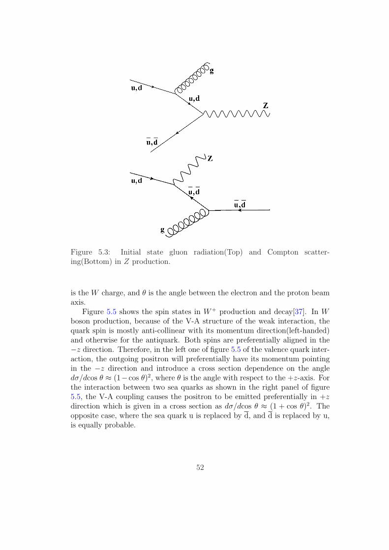
Figure 5.3: Initial state gluon radiation(Top) and Compton scatter-ing(Bottom) in Z production.
is the W charge, and θ is the angle between the electron and the proton beamaxis.
Figure 5.5 shows the spin states in W+ production and decay[37]. In Wboson production, because of the V-A structure of the weak interaction, thequark spin is mostly anti-collinear with its momentum direction(left-handed)and otherwise for the antiquark. Both spins are preferentially aligned in the−z direction. Therefore, in the left one of figure 5.5 of the valence quark inter-action, the outgoing positron will preferentially have its momentum pointingin the −z direction and introduce a cross section dependence on the angledσ/dcos θ ≈ (1−cos θ)2, where θ is the angle with respect to the +z-axis. Forthe interaction between two sea quarks as shown in the right panel of figure5.5, the V-A coupling causes the positron to be emitted preferentially in +zdirection which is given in a cross section as dσ/dcos θ ≈ (1 + cos θ)2. Theopposite case, where the sea quark u is replaced by d, and d is replaced by u,is equally probable.
52

Figure 5.4: Leading order W (Z) boson production and decay
5.2 Boson pT
As discussed in chapter 3, the W boson pT spectrum has a significant impacton the simulated pT (e) and /ET spectra so an accurate description of this isan important ingredient of the W mass measurement. We used RESBOS [41]to simulate the boson production and decay process, which gives reasonabledescription of the transverse momentum of the vector bosons. It extends theCollins-Soper-Sterman resummation formalism[42], for on-shell vector bosonproduction, to correctly include the effects of the polarization and the width ofthe vector boson to the distributions of the decay leptons. RESBOS computesthe triple differential cross section d3σ/dpT dy dm for Z/γ∗ and W processesat hadron colliders, where pT is the boson momentum in the plane transverseto the beam, y = 1
2ln[(E + pz)/(E − pz)] is the boson rapidity and m is the
boson mass. It uses a gluon resummation calculation for low boson transversemomentum pT and perturbative QCD calculations at high boson pT .
For low pT W and Z bosons, the main higher order correction to the overallcross section comes from multiple soft and collinear gluon emission which iscalculated using a gluon resummation technique. In impact-parameter spaceresummations, the W pT spectrum is parametrized using a non-perturbativeform-factor using three parameters called g1, g2 and g3. The values of thesethree parameters need to be determined from experimental data. The Z bosonpT distribution at the Fermilab Tevatron is by far the most sensitive to thevalue of g2, has limited sensitivity to g1, and is quite insensitive to the valueof g3. We use the global fit values listed at Ref. [43] with g2 = 0.68 ± 0.02and propagate the uncertainty on g2 to the W mass measurement. The un-
53

Figure 5.5: Spin states for W+ production and decay. Left: W+ producedwith valence quarks; Right : One of the cases of W+ production with seaquarks.(The opposite case with sea quark u and d switched with each other isequally probable.)
certainties from g1 and g3 are negligible. Figure 5.6 shows the propagation ofthe error on g2 to the measured value of the W mass uncertainty.
Table 5.1 lists the corresponding propagated uncertainty on the W mass.
mT fit pT (e) fit /ET fit
∆MW /∆g2(MeV ) 101 243 79∆MW (MeV) 2 5 2
Table 5.1: Systematic uncertainty on W mass measurement due to g2 uncer-tainty.
5.3 PDF
The partonic structure of hadrons plays a fundamental role in elementary par-ticle physics. Parton distribution functions (PDFs) enter into the W massmeasurement through their effects on the detector acceptance and kinemat-ics of the decay electron. The PDFs are determined phenomenologically bya global analysis of experimental data from a wide range of hard-scatteringprocesses, such as deep inelastic scattering, jet production and the W chargeasymmetry. The PDFs are specified in a parameterized form at a fixed low
54

Figure 5.6: The corresponding MW error versus g2: top for mT and bottomfor pT (e) methods respectively
55

energy scale(1 GeV), from which the PDFs at high energies are determined byNLO perturbative QCD. CTEQ uses an effective global χ2 function to mea-sure the quality of the fit between theory and experiment. The global χ2 iscalculated by using 15 data sets from 15 differents experiments around theworld. To study the uncertainties of PDF’s, the variation of χ2 is explored inthe neighborhood of its minimum.
We determine the systematic uncertainty arising from the PDFs using astandard prescription for the CTEQ6.1M [44] parton distribution function.We used pythia to generate W → eν events using the central PDF set.After passing through fast MC simulation and event selection, those eventswere treated as “data”. Then we use the standard PDF reweighting methodto generate mass templates for different ”theories” involving variation of thePDF’s. By performing the PDF reweighting, the statistical impact is mini-mized. There are 20 free parameters in the CTEQ6.1M PDF set. For theuncertainty calculation, 40 additional sets were defined by positive and nega-tive variation of each parameter until the global χ2 reached the 90% C.L. Thedefault values of W mass and width used in pythia are 80.450 GeV and 2.071GeV respectively. For each PDF set, we generated 100 MW templates centeredat 80.450 GeV with a step size of 2 MeV. To determine each mass shift, wecalculate the binned log-likelihood for the mT (or pT (e), /ET ) distribution usingthe central PDF and the 100 MW templates for each of 40 PDF sets[45].
We use the following formula to obtain the uncertainty with 68% C.L. [46]:
∆MW =1
2× 1.6
√√√√20∑i=1
(M+i −M−
i )2 (5.4)
where M+i and M−
i are the W masses determined using the ith uncertaintyPDF sets. The factor 1.6 is used to convert from a 90% confidence interval tothe more standard 68% confidence interval.
We did the same analysis using pT (e) and /ET methods. The final uncer-tainty is found to be 10 MeV for mT method, 11 MeV for pT (e) method and11 MeV for the /ET method[47].
5.4 Electroweak Corrections
Radiation from the decay electron or the W boson biases the mass measure-ment. W or Z decays into leptons (+neutrino) through electro-weak interac-tions.
56

q′q → W → lν(γ) (5.5)
qq → Z → ll(γ) (5.6)
There is a certain probability that an electron will radiate a photon, whichwill take away some of the energy of the electron. The invariant mass of leptons(or lepton + neutrino) is lower than the original boson. The radiated photonsare often collinear with the electrons and reconstructed as the same EM cluster,so modeling the photon radiation in generator and the fast simulation plays acrucial role in measuring the W mass.
The EW contributions to the W mass uncertainty mainly come from thefollowing sources:
• photon radiation off the incoming quarks
• photon radiation off the W propagator
• photon radiation off the final-state electron (the most important contri-bution)
• all other EW processes: virtual corrections via photons or Z bosons
The dominant effect from EW corrections to the W mass measurementcomes from radiation of a single photon from the final state charged lepton.The next-largest effect is due to two final state photon radiations. These pro-cesses are simulated by combining the PHOTOS program [48] with RESBOS.
PHOTOS is a universal Monte Carlo event generator simulating QED final-state radiation corrections in decays of particles and resonances. It takes theRESBOS output as the input to add the final state radiation and can radiateup to two photons off one electron.
The photon energy cut, controlled by the input parameter δs, is made onthe fraction of the parton’s energy carried by the emitted photon in the parton-parton center of mass system. Events with photon energy below the cut willbe thrown away:
Eγ > δs
√s/2 (5.7)
where√
s is the parton energy in the parton-parton center-of-mass system.So δs = 0.001 corresponds to the energy Eγ = 40 MeV. Events with photon
Eγ < δs
√s/2 are considered as two-body events.
In order to study the effect of varying the photon energy cut, we changeδs from 0.00025 to 0.02, corresponding the minimum photon energy from 10MeV to 800 MeV[49]. We run RESBOS+PHOTOS with variant δs, then go
57

δs Eγcut ∆MW ∆MW ∆MW ∆MZ ∆(MW
MZ) ∆(MW
MZ) ∆(MW
MZ)
(× (MeV) (mT ) (pT (e)) (/ET ) (Z Mass) (mT ) (pT (e)) (/ET )10−3) (MeV) (MeV) (MeV) (MeV) (×10−5) (×10−5) (×10−5)0.25 10 -25 ± 3 -23 ± 4 -22 ± 4 -34 ± 2 5.5 7.7 8.80.5 20 -29 -29 -27 -30 -2.8 -2.8 -0.60.6 24 -24 -27 -24 -32 4.6 1.3 4.60.7 28 -24 -29 -19 -32 4.6 -0.85 10.00.8 32 -21 -23 -20 -33 8.9 6.7 10.01 40 -20 -20 -20 -27 4.2 4.2 4.23 120 -17 -22 -14 -21 1.7 -3.8 5.05 200 -10 -13 -12 -15 3.5 0.25 1.310 400 0 0 0 0 0 0 015 600 5 8 6 11 -5.2 -1.9 -4.120 800 18 20 15 26 -5.4 -3.2 -8.7
Table 5.2: Mass shift of W and Z due to δs variation.
through the fast simulation, and fit the output using the mass templates withδs=0.01. δs=0.01 is the default value in our simulation. The variation rangefrom 0.00025 to 0.02 well covers the default value. We also go through thesame procedure for Z boson.
Table 5.2 shows the mass shifts of W and Z, and their mass ratio. Aswe lower the photon cut, more events will have FSR, so the W and Z masswill shift lower. Among three methods using mT , pT (e) and /ET , the methodpT (e) is most affected just as we expected. Z mass is more vulnerable to thephoto radiation because it decays into two electrons and its mass heavily relieson the reconstructed electron energy. Since we use Z → ee events to do thecalibration, what really matters is the W/Z mass ratio. We plot the mass ratioversus the photon energy cut and fit the plots with a flat line that gives a goodχ2/d.o.f . We take the fitted value multiplied by the Z mass to estimate theW mass uncertainty due the photon energy cut. So it introduces 2 MeV(mT ),1 MeV(pT (e)) and 3 MeV(/ET ) into the W mass uncertainty.
The effect of the minimum distance between the radiated photon andthe electron on the W mass measurement is negligible. We study the ef-fects of ISR, ISR-FSR interference and other EW corrections by using thewgrad(zgrad)[50][51] program. wgrad(zgrad) provides an option thatallows us to include FSR-only correction or the full electroweak corrections.By turning on and off this option and letting the generated events pass throughthe fast simulation, we measure the relative W mass shift between the two op-
58

cone ∆MW ∆MW ∆MW ∆MZ ∆(MW
MZ) ∆(MW
MZ) ∆(MW
MZ)
size (mT ) (pT (e)) (/ET ) (Z Mass) (mT ) (pT (e)) (/ET )(MeV) (MeV) (MeV) (MeV) (×10−5) (×10−5) (×10−5)
0.2 -18±3 -16±4 -8±4 -21±2 0.57 2.8 11.50.25 -7 -8 -1 -6 -1.9 -3.0 4.70.3 0 0 0 0 0 0 00.35 6 7 0 7 -0.19 0.9 -6.80.4 12 15 3 16 -2.3 0.98 -12.2
Table 5.3: Mass shift of W or Z due to change of photon merge cone size
tions, which is taken as the uncertainty due to the effect of ISR, ISR-FSRinterference and other EW corrections. The final uncertainty is found to be 5MeV for mT method, 5 MeV for pT (e) method and 5 MeV for /ET method.
Besides the uncertainty that comes from the theoretical prediction on pho-ton radiation, our treatment of radiated photons could also give us some biases.If a radiated photon is close to the electron, it will deposit most of its energy inthe electron shower, which we need to take into account in our fast simulation.Here is how we treat photons in the fast simulation. If a photon is within the0.3 cone around an electron, it will be merged into this electron and removedfrom the recoil system, otherwise it will be kept in the recoil system. The 0.3photon merge cone size will bring up some uncertainty into W mass becausesome photons will change the electron shower shape and not be reconstructedas an EM object.
To quantify the impact of photon merge cone size change, we vary the conesize as 0.2, 0.25, 0.3, 0.35, 0.4 to see W and Z mass shift. Table 5.3 lists themass shifts of W and Z. From the table, one can see that the W values ofpT (e) and mT are quite sensitive to the change of cone size while /ET is notvery sensitive. This is what we expected. The Z mass is even more sensitiveto the change of cone size because in each Z event there are two electrons, andtherefore the Z is more likely to have FSR than the W . Figure 5.7, shows theratio of fitted W mass to Z mass versus cone size using mT , pT (e) and /ET . Theratio is fit with a horizontal line, and the uncertainty propagated into the Wmass results in uncertainties 1 Mev, 1 MeV and 5 MeV. As discussed before,W pT (e), mT and Z Mass are all sensitive to the cone size change. When wetake the ratio between W and Z, the uncertainties cancel each other. /ET isnot sensitive to the cone size change, so its uncertainty does not cancel withthe uncertainty in the Z mass as well.
59

Merge-Cone Size0.2 0.25 0.3 0.35 0.4
-0.06
-0.04
-0.02
0
0.02
0.04
-310×p0 7.44e-05± 1.689e-05 p1 0.0002414± -8.17e-05 p0 7.44e-05± 1.689e-05 p1 0.0002414± -8.17e-05
Tratio: W mass / Z mass using M
Merge-Cone Size0.2 0.25 0.3 0.35 0.4
-0.08
-0.06
-0.04
-0.02
0
0.02
0.04
0.06
0.08
-310×p0 9.345e-05± 1.554e-06 p1 0.0003032± 5.989e-06 p0 9.345e-05± 1.554e-06 p1 0.0003032± 5.989e-06
(e)T
ratio: W mass / Z mass using p
Merge-Cone Size0.2 0.25 0.3 0.35 0.4-0.2
-0.15
-0.1
-0.05
0
0.05
0.1
0.15
-310×p0 9.345e-05± 0.0003481 p1 0.0003032± -0.001178 p0 9.345e-05± 0.0003481 p1 0.0003032± -0.001178
ratio: W mass / Z mass using MET
Figure 5.7: Mass ratio (W/Z) vs Photon Merge Cone Size: mT (top),pT (e)(middle) and /ET (bottom)
60

Chapter 6
Efficiency
A set of selection criteria are used to select electrons and events. These criteriaare powerful in rejecting the background. Meanwhile, they can also reject somegood electrons and W (Z) events. However, the reason the efficiency is impor-tant is not in its absolute value, but in its different dependencies, especiallythe kinematic dependencies(for example, the pT (e) dependence). It is the de-pendence that will shape the final spectrum of the three variables(MT , pT (e)and /ET ) we are using to measure the W boson mass. Because of the existenceof crack in the detector, we can only reconstruct events with electrons pointinginto the fiducial region, which defines the geometric acceptance. The imperfec-tion of the detector introduces the angular dependence of the efficiency, whichis not only important to the kinematic variables, but also crucial to the EMenergy resolution. Aside from the intrinsic pT (e) dependence, the efficiencyis also subject to effects from the recoil system(both the relative directionand the absolute magnitude of the energy from the rest of the event). Thefact we are using not just one selection criteria requires some extra measures,since different criteria have different sensitivities. The SMT hit requirementis extremely sensitive to the primary vertex z-component due to the limitedcoverage of SMT, while the variables based on the calorimeter information isfree from this problem.
To study the efficiency in the data, a method called tag-and-probe [52]is used on the Z → ee events. The basic idea is we require one of the twoelectrons(tag) to pass all the standard selection cuts, and also require theother electron(probe) to pass all the selection cuts except the one we want tostudy(for example, the track match). We also require the invariant mass ofthe tag and probe electron to be in the neighborhood of the well-known Zmass(70 GeV< Mee < 110 GeV). By means of this, we have a good handle onselecting good Z → ee electrons. Then the probe electron is used to measurethe efficiency. The two electrons can switch their roles in being the tag or
61

probe, in some cases.
6.1 Geometric Acceptance
There are 32 EM modules in the φ direction of the central calorimeter, eachmodule is 2π/32 ∼ 0.2 radian wide in φ. An intra-module φ variable, PhiMod,is defined as fmod1(32φ/2π, 1.0) with 0 ≤ phiMod < 1. In the region of inter-modular boundaries or gaps better known as the “φ cracks”, we have lesscalorimeter signal response. We exclude these regions in the data selection.so 20% of the azimuthal CC phase space is removed. At fixed ηdet each ofthe EM1, EM2 and EM4 layers in an EM module consists of 2 read out cells.The central value of PhiMod=0.5 corresponds to the inter-cell boundary, thevalues close to 0 and 1 are the module edges. The EM3 layer is segmentedtwice as finely in both eta and phi (0.05 radian wide). Thus in an EM modulethis layer contains 8 ‘readout cells’ at a “fixed ηdet” each with a width of 0.05.
Due to the EM clustering algorithms and the electronics, the electron clus-ter angle φEM calculated from the electron energy deposited in the third EMlayer is biased towards the center of the module [53]. Figure 6.1 (Left) showsthe PhiMod bias vs the PhiMod of the extrapolated track position across themodule (fmod(32φtrk/2π, 1.0)). Since φtrk is unbiased, we can see a strongtendency for the φEM to move towards the center of the module.
Due to the arrangement of the electrode pads in the calorimeter, the effi-ciency to find electron clusters varies with the φ of the incident particle [54].Figure 6.1 (Right) shows the efficiency of finding an EM cluster vs PhiMod indata. For the final analysis, we only keep electrons with 0.1 < PhiMod < 0.9.
Understanding both the efficiency and the bias is important for modelingthe Z boson transverse momentum distribution in the fast simulation andfurther impact the electron pT and recoil system pT distributions. Both theefficiency and the bias are measured using electrons from Z → ee events.
6.2 Trigger Efficiency
The data used for this measurement was collected from 2002 to 2006, coveringover four trigger periods, and the L1/L2/L3 requirements are different fordifferent periods. The trigger efficiency is measured using the tag-and-probemethod on Z → ee events. To pass the trigger requirement, an electronshould have a matching trigger object at each level which passes all cuts for
1fmod(numerator,denominator) is the floating-point remainder of numera-tor/denominator.
62
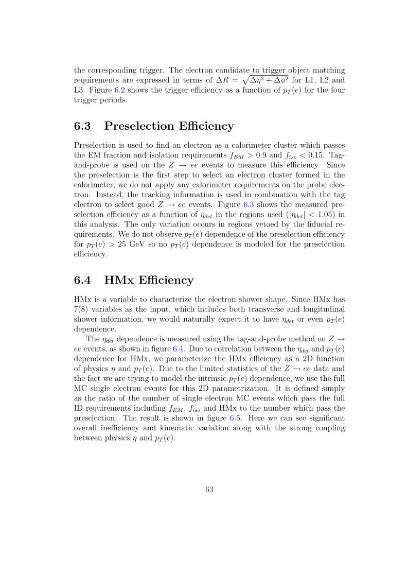
the corresponding trigger. The electron candidate to trigger object matchingrequirements are expressed in terms of ∆R =
√∆η2 + ∆φ2 for L1, L2 and
L3. Figure 6.2 shows the trigger efficiency as a function of pT (e) for the fourtrigger periods.
6.3 Preselection Efficiency
Preselection is used to find an electron as a calorimeter cluster which passesthe EM fraction and isolation requirements fEM > 0.9 and fiso < 0.15. Tag-and-probe is used on the Z → ee events to measure this efficiency. Sincethe preselection is the first step to select an electron cluster formed in thecalorimeter, we do not apply any calorimeter requirements on the probe elec-tron. Instead, the tracking information is used in combination with the tagelectron to select good Z → ee events. Figure 6.3 shows the measured pre-selection efficiency as a function of ηdet in the regions used (|ηdet| < 1.05) inthis analysis. The only variation occurs in regions vetoed by the fiducial re-quirements. We do not observe pT (e) dependence of the preselection efficiencyfor pT (e) > 25 GeV so no pT (e) dependence is modeled for the preselectionefficiency.
6.4 HMx Efficiency
HMx is a variable to characterize the electron shower shape. Since HMx has7(8) variables as the input, which includes both transverse and longitudinalshower information, we would naturally expect it to have ηdet or even pT (e)dependence.
The ηdet dependence is measured using the tag-and-probe method on Z →ee events, as shown in figure 6.4. Due to correlation between the ηdet and pT (e)dependence for HMx, we parameterize the HMx efficiency as a 2D functionof physics η and pT (e). Due to the limited statistics of the Z → ee data andthe fact we are trying to model the intrinsic pT (e) dependence, we use the fullMC single electron events for this 2D parametrization. It is defined simplyas the ratio of the number of single electron MC events which pass the fullID requirements including fEM , fiso and HMx to the number which pass thepreselection. The result is shown in figure 6.5. Here we can see significantoverall inefficiency and kinematic variation along with the strong couplingbetween physics η and pT (e).
63

6.5 Tracking Efficiency
The track-matching requirement is the spatial track match plus at least oneSMT hit and does not include the the track pT cut. The tracking resolutionand pT cut are modeled separately in the fast MC. As briefly discussed atthe beginning of this chapter, the limited SMT coverage introduces a strongcoupling between the ηphys and primary vertex z position for the trackingefficiency, which is measured using the tag-and-probe on the Z → ee data, asshown in figure 6.6.
To determine the dependence of the tracking efficiency on electron pT andηphys , the same single electron full MC sample is used as previously. Similar tothe HMx efficiency, the tracking efficiency is a relative efficiency, defined as theefficiency with which an electron that passes all of the calorimetric (EMID)requirements also passes the track-matching requirement. Figure 6.7 showsthe tracking efficiency as a function of pT (e) for different ηphys bins.
6.6 u||(Recoil Related) Efficiency
Among the electron selection cuts, isolation, HMx and track match are heavilyaffected by the recoil system, which is mainly composed of hadronic jets, alongwith the residuals from spectator parton interaction, electron noise and pileupfrom previous bunches. When the recoil system is not too far from the electron,it will change the electron shower shape and its isolation value. The recoilsystem also brings tracks, and therefore affects the track match. The projectionof the recoil pT to the electron transverse direction, u‖, is used to parameterizethe recoil effect on the electron selection criteria (electron isolation, HMx andtrack matching).
First, it is important to understand the u|| efficiency difference [55] in Z andW events, I will present the discussion using the full MC events. To measurethe u‖ efficiency in full MC, we used two different methods: the truth methodand the tag-and-probe method. For the truth method, since in the full MCsamples we know we have true electron(s) which decay from the Z or W boson,we simply remove the cuts under study (isolation, HMx and track matching),and then apply those cuts to determine the efficiency. We did this for both Wand Z full MC samples. For the tag-probe method, we only can use Z → eeevents. We require one tag electron that passes tighter selection cuts, and thencheck the second electron. This method can be applied for real data analysiswhere the truth information is not available, although background subtractionis needed.
Figure 6.8 shows the u‖ efficiency using the truth and tag-and-probe method
64

p0 p1 p2
(GeV) (GeV−1)Z → ee(truth) 1.473 ± 0.272 0.0071 ± 0.0004 0.8336 ± 0.0006Z → ee(tag-probe) 1.510 ± 0.290 0.0070 ± 0.0005 0.8442 ± 0.0007W → eν(truth) 1.064 ± 0.156 0.0078 ± 0.0003 0.8260 ± 0.0004W → eν(truth: fix p0) 1.473(fixed) 0.0083 ± 0.0002 0.8255 ± 0.0004
Table 6.1: p0, p1, p2 of Z → ee and W → eν
in Z → ee events. The distribution is fitted with a function of the form:
ε(u‖) = p2
1 for u‖ < p0
1− p1(u‖ − p0) otherwise(6.1)
The parameter p2 is an overall efficiency (εiso× εHMx× εtrk), p0 is the valueof u‖ at which the efficiency starts to decrease as a function of u‖, and p1 is therate of decrease. If u‖ is negative, the efficiency is basically flat because therecoil system and the electron are on the opposite hemisphere, and thus therecoil system has little effect on the electron identification. Once u‖ is greaterthan p0, the recoil system is getting closer to the electron and starts to distortthe electron identification. The more positive u‖ gets, the lower efficiency theelectron will be found at. The slope parameter p1 indicates how the electronselection will be affected by the recoil system. The fitted parameters using thetruth method and tag-probe method are listed in table 6.1. The parametervalues in table 6.1 clearly demonstrate the two methods give very consistentresults, which means eventually we could use the tag-probe method whendealing with the data.
Figure 6.9 shows the u‖ efficiency using the truth method in W → eνevents. The fitted values are also listed in table 6.1. In figure 6.9, the leftone allows the parameter p0, the turning point, to float, which gives the slopep1 = 0.0078 ± 0.0003 GeV−1, about 1.4σ larger than p1 = 0.0071 ± 0.0004GeV−1 obtained from Z . However, we also notice the turning point is differentbetween Z and W , which is highly correlated with the slope. To really comparethe slopes obtained from Z and W , we fix the turning point at the same value.The right plot in Fig. 6.9 shows the same distribution as the left one, but withfixing the turning point p0 at the value obtained from Z (left plot in Fig. 6.8).We find that the slope for W is even bigger with p1 = 0.0083± 0.0002 GeV−1,2.7σ larger than p1 in Z.
One might wonder why Z and W give different u|| slope. The left picturein Fig.6.10 shows an event of Z → ee. When we shrink each vector in this
65

p0 p1 p2
(GeV) (GeV−1)Z → ee(truth) 1.137 ± 0.231 0.0077 ± 0.0004 0.8338 ± 0.0007Z → ee(tag-probe) 1.192 ± 0.247 0.0076 ± 0.0005 0.8443 ± 0.0007W → eν(truth) 1.064 ± 0.156 0.0078 ± 0.0003 0.8260 ± 0.0004W → eν(truth: fix p0) 1.137(fixed) 0.0078 ± 0.0002 0.8259 ± 0.0004
Table 6.2: p0, p1, p2 of Z → ee after scaled to W and W → eν
event by a factor 80.419/90.188, i.e. the boson mass ratio, and replace one ofthe electrons by a neutrino, we then get a W → eν event, as shown in the righthand picture. So the open angle between the electron and the hard recoil andtheir energy ratio is the same in the two pictures. On the first (linear) orderapproximation, we would expect the electrons in this particular Z and W eventhave the same efficiency. However, the hard recoil system in W event is softer,therefore gives a smaller u|| when projected onto the electron direction. Thistranslates into the fact that W u|| efficiency presents a smaller turning pointand steeper slope, as we have just seen. So if we scale the u|| in Z by a factor80.419/90.188, we should be able to get the same u|| efficiency as W. Fig.6.11shows the Z u|| efficiency using the truth and tag-probe method after scalingto the W . Table 6.2 lists the new fitted parameters from Z by scaling it toW and the original values from W . These numbers clearly show the turningpoint and slope values from scaled Z agree very well with W .
We have been focusing on p0 and p1 because we only care about the turningpoint and the slope when parameterizing the efficiency in the fast simulation.However, we also have the plateau(p2) difference between Z and W , and evenbetween the truth and tag-and-probe method in Z. For Z events, the efficiencyplateau difference between the truth and tag-and-probe method is about 1%,which is reasonable since we have a 2%[52] systematic bias due to this tag-and-probe method. As we have previously mentioned, when we transfer for aZ event to a W event, the hard component of the recoil system gets softer.But the soft component of the recoil system is approximately the same for Zand W , which is composed of the spectator parton interaction, electronic noiseand pileup, etc. Since W electrons are softer than Z electrons on average, Welectrons are more affected by the soft recoil and show a slightly lower averageefficiency.
When we model the u|| efficiency in the fast simulation, however, we needto make a little adjustment. In the fast simulation, we also model the purepT (e) dependence of the track match and HMx by studying the full MC single
66

electron events that have no recoil. The u|| efficiency, measured from full MCwith the recoil, essentially consists of both the pure pT (e) dependence andthe recoil effect. When modeling the pT (e) and the u|| efficiency simultane-ously in the fast simulation, the double counting of the pure pT (e) dependenceneeds to be removed. To do the double counting removing, we perform thesame procedure in the fast simulation as in full MC to measure the u|| effi-ciency and compare it with the one we got from full MC. By adjusting the u||efficiency slope we put in the fast simulation, we can obtain the best agree-ment between full and fast simulation on the u|| efficiency. This way we canget the adjusted u|| efficiency slope for the fast simulation that is after thedouble-count-removing.
6.7 SET(Overall Hadronic Activity) Efficiency
The “rest of the event” mainly consists of hadronic activity from the spectatorpartons, additional pp interactions and the hadronic recoil that balances thevector boson. It has an important impact on the electron reconstruction andidentification efficiency. SET(Scalar Transverse Energy) is a good observableto reflect the effects from the overall hadronic energy in an event. It basicallyaccounts for the magnitude of activity in the rest of the event. The effectrelated to the relative direction between the electron and the rest of the eventis parameterized using u||.
Standard full MC plus overlay of collider data events are used to constructthe SET efficiency model. The efficiency is parameterized versus the SET fromthe overlay of ZB events and applied to the total SET in the event. Z → eefull MC events passing the standard selection without recoil pT requirementare used to derive the per-event reconstruction efficiency as a function of theSET of the ZB event used for overlay. The efficiency is defined as the numberof selected events divided by the total as a function of SET. The measuredSET efficiencies, separately for full MC Z and W events, are smoothed usinga polynomial function with coefficients by fitting the efficiency versus SEThistogram, shown in figure 6.12.
The higher pT electron is more likely to survive the “rest of the event”tobe reconstructed and pass the selection requirement. So we introduce a smallmultiplicative correction factor to the per-event efficiency depending on pT (e)and SET in the case of W → eν and two multiplicative correction factors(one per electron) in the case of Z → ee. The same procedure is followed asthe simple model above to derive the per-electron perturbations. But now weperform the analysis in bins of reconstructed electron pT . Figure 6.13 showsper-electron correction factors for the W → eν events. The correction factor
67

is multiplied to the SET efficiency shown in figure 6.12. We can see electronswith high pT (> 60 GeV) need a correction factor greater than 1 for the reasonmentioned above.
6.8 Final Efficiency Check
So far as we discussed, the geometric dependencies are measured using thetag-and-probe method on the Z → ee data. For the pT (e) related dependence,different full MC samples have been largely used. For example, the correlationsbetween the electron pT , the electron physics η and the event SET are studiedand modeled in detail in the fast simulation. Due to the truth method we areusing for the full MC and the limited statistics in the data, the correspondingprocedure and binning in η/pT (e) can not be repeated in the data. Since thefast simulation has been tuned to describe the detailed MC well, the best thingto do is to check if there is any difference between the data and full MC whenit comes to the pT (e) dependence of the selection efficiency. In case there isany difference, we can correct the efficiency measured in full MC by the ratiobetween the data and full MC. We perform the tag-and-probe method in boththe data and full MC to measure the pT dependence. Figure 6.14 shows thepT dependence of the HMx efficiency for CC electrons in the data and fullMC(left) and their ratio(right). It clearly demonstrates that the data andfull MC have the same pT dependence to within the errors from limited datastatistics, and we can simply fit their ratio by a flat line with a good χ2/dof.We observe a similar behavior for the track match, as shown in figure 6.15.Given these results, we can now securely rely on the pT dependence measuredfrom full MC for the data measurement.
68

Extrapolated track PhiMod0 0.2 0.4 0.6 0.8 1
π)/
2tr
kφ-
EM
φ32
(
-0.2
-0.1
0
0.1
0.2 Entries 57240Mean x 0.4991Mean y 0.00235RMS x 0.2759RMS y 0.02609
Entries 57240Mean x 0.4991Mean y 0.00235RMS x 0.2759RMS y 0.02609
Extrapolated track PhiMod0 0.2 0.4 0.6 0.8 1
Ph
iMo
d e
ff
0.4
0.6
0.8
1
Figure 6.1: Top: Difference between φEM and φtrk (fmod(32(φEM −φtrk)/2π, 1.0))in module units vs track phimod (fmod(32φtrk/2π, 1.0)). Bottom: PhiMod efficiencyas a function of the extrapolated track PhiMod.
69

pT [GeV]0 20 40 60 80
Eff
icie
ncy
0
0.2
0.4
0.6
0.8
1
pT [GeV]0 20 40 60 80
Eff
icie
ncy
0
0.2
0.4
0.6
0.8
1
pT [GeV]0 20 40 60 80
Eff
icie
ncy
0
0.2
0.4
0.6
0.8
1
pT [GeV]0 20 40 60 80
Eff
icie
ncy
0
0.2
0.4
0.6
0.8
1
Figure 6.2: Trigger efficiency vs electron pT for four different trigger periods.Top left: v8-11, top right: v12, bottom left: v13 and bottom right: v14.
detηElectron
-3 -2 -1 0 1 2 3
Eff
icie
ncy
0.8
0.85
0.9
0.95
1
Figure 6.3: The efficiency for reconstructing a loose EM cluster. The efficiencyis almost flat over the η region used here (|ηdet| < 1.05).
70

detηElectron
-3 -2 -1 0 1 2 3
Eff
icie
ncy
0.85
0.9
0.95
Figure 6.4: The ηdet dependence of the final HMx requirements relative to thepreselection.
71

pT, GeV20 40 60 80 100
0.6
0.7
0.8
0.9
1
1.1 < -1.1η-1.3 <
pT, GeV20 40 60 80 100
0.6
0.7
0.8
0.9
1
1.1 < -0.9η-1.1 <
pT, GeV20 40 60 80 100
0.6
0.7
0.8
0.9
1
1.1 < -0.7η-0.9 <
pT, GeV20 40 60 80 100
0.6
0.7
0.8
0.9
1
1.1 < -0.5η-0.7 <
pT, GeV20 40 60 80 100
0.6
0.7
0.8
0.9
1
1.1 < -0.3η-0.5 <
pT, GeV20 40 60 80 100
0.6
0.7
0.8
0.9
1
1.1 < -0.1η-0.3 <
pT, GeV20 40 60 80 100
0.6
0.7
0.8
0.9
1
1.1 < 0.1η-0.1 <
pT, GeV20 40 60 80 100
0.6
0.7
0.8
0.9
1
1.1 < 0.3η0.1 <
pT, GeV20 40 60 80 100
0.6
0.7
0.8
0.9
1
1.1 < 0.5η0.3 <
pT, GeV20 40 60 80 100
0.6
0.7
0.8
0.9
1
1.1 < 0.7η0.5 <
pT, GeV20 40 60 80 100
0.6
0.7
0.8
0.9
1
1.1 < 0.9η0.7 <
pT, GeV20 40 60 80 100
0.6
0.7
0.8
0.9
1
1.1 < 1.1η0.9 <
pT, GeV20 40 60 80 100
0.6
0.7
0.8
0.9
1
1.1 < 1.3η1.1 <
Figure 6.5: The η and pT dependence of the HMx efficiency for single electronsrelative to the preselection efficiency. Each pane shows the pT efficiency in agiven η bin. The bins are 0.2 units wide in η and cover the range −1.3 ≤ η ≤1.3, and the horizontal axes run from 20 GeV to 100 GeV.
72

-60-40
-200
2040
60
-3-2
-10
12
30
0.2
0.4
0.6
0.8
1
-60 -40 -20 0 20 40 60-2
-1.5
-1
-0.5
0
0.5
1
1.5
2
Figure 6.6: The tracking efficiency as a function of ηphys and vertex z positionshown as a lego plot(top) and as a box plot(bottom).
73

pT, GeV20 40 60 80 100
0.6
0.7
0.8
0.9
1
1.1 < -1.1η-1.3 <
pT, GeV20 40 60 80 100
0.6
0.7
0.8
0.9
1
1.1 < -0.9η-1.1 <
pT, GeV20 40 60 80 100
0.6
0.7
0.8
0.9
1
1.1 < -0.7η-0.9 <
pT, GeV20 40 60 80 100
0.6
0.7
0.8
0.9
1
1.1 < -0.5η-0.7 <
pT, GeV20 40 60 80 100
0.6
0.7
0.8
0.9
1
1.1 < -0.3η-0.5 <
pT, GeV20 40 60 80 100
0.6
0.7
0.8
0.9
1
1.1 < -0.1η-0.3 <
pT, GeV20 40 60 80 100
0.6
0.7
0.8
0.9
1
1.1 < 0.1η-0.1 <
pT, GeV20 40 60 80 100
0.6
0.7
0.8
0.9
1
1.1 < 0.3η0.1 <
pT, GeV20 40 60 80 100
0.6
0.7
0.8
0.9
1
1.1 < 0.5η0.3 <
pT, GeV20 40 60 80 100
0.6
0.7
0.8
0.9
1
1.1 < 0.7η0.5 <
pT, GeV20 40 60 80 100
0.6
0.7
0.8
0.9
1
1.1 < 0.9η0.7 <
pT, GeV20 40 60 80 100
0.6
0.7
0.8
0.9
1
1.1 < 1.1η0.9 <
pT, GeV20 40 60 80 100
0.6
0.7
0.8
0.9
1
1.1 < 1.3η1.1 <
Figure 6.7: The tracking efficiency as a function of η and pT determined usingsingle electron events. Each panel shows the pT efficiency in a given η bin.The η bins are 0.2 η-units wide and cover the range −1.3 ≤ η ≤ 1.3, and thehorizontal axis in each figure runs from 20 GeV to 100 GeV.
74

/ ndf 2χ 77.37 / 57Prob 0.03761p0 0.272± 1.473 p1 0.000427± 0.007085 p2 0.0006± 0.8336
(GeV)||u-30 -20 -10 0 10 20 300.6
0.65
0.7
0.75
0.8
0.85
0.9
0.95
1 / ndf 2χ 77.37 / 57Prob 0.03761p0 0.272± 1.473 p1 0.000427± 0.007085 p2 0.0006± 0.8336
/ ndf 2χ 58.51 / 57Prob 0.4199p0 0.29± 1.51 p1 0.000457± 0.007041 p2 0.0007± 0.8442
(GeV)||u-30 -20 -10 0 10 20 300.6
0.65
0.7
0.75
0.8
0.85
0.9
0.95
1 / ndf 2χ 58.51 / 57Prob 0.4199p0 0.29± 1.51 p1 0.000457± 0.007041 p2 0.0007± 0.8442
Figure 6.8: u‖ efficiency in full MC Z → ee: Top: Truth method; Bottom:tag-probe method
75

/ ndf 2χ 101.7 / 57p0 0.156± 1.064 p1 0.000278± 0.007758 p2 0.000± 0.826
(GeV)||u-30 -20 -10 0 10 20 300.6
0.65
0.7
0.75
0.8
0.85
0.9
0.95
1 / ndf 2χ 101.7 / 57
p0 0.156± 1.064 p1 0.000278± 0.007758 p2 0.0004 ± 0.8260
/ ndf 2χ 106.2 / 58
p1 0.000222± 0.008258
p2 0.0004± 0.8255
(GeV)||u-30 -20 -10 0 10 20 300.6
0.65
0.7
0.75
0.8
0.85
0.9
0.95
1 / ndf 2χ 106.2 / 58
p1 0.000222± 0.008258
p2 0.0004± 0.8255
Figure 6.9: u‖ efficiency in full MC W → eν using truth method: Top: allowp0 to float; Bottom: fix p0 the same as for Z
76

Figure 6.10: Left:Z → ee; Right:W → eν
77

/ ndf 2χ 76.42 / 57p0 0.231± 1.137 p1 0.000423± 0.007666 p2 0.0007± 0.8338
(GeV)||u-30 -20 -10 0 10 20 300.6
0.65
0.7
0.75
0.8
0.85
0.9
0.95
1 / ndf 2χ 76.42 / 57
p0 0.231± 1.137 p1 0.000423± 0.007666 p2 0.0007± 0.8338
/ ndf 2χ 64.88 / 57p0 0.247± 1.192 p1 0.000452± 0.007606 p2 0.0007± 0.8443
(GeV)||u-30 -20 -10 0 10 20 300.6
0.65
0.7
0.75
0.8
0.85
0.9
0.95
1 / ndf 2χ 64.88 / 57
p0 0.247± 1.192 p1 0.000452± 0.007606 p2 0.0007± 0.8443
/ ndf 2χ 101.7 / 57p0 0.156± 1.064 p1 0.000278± 0.007758 p2 0.000± 0.826
(GeV)||u-30 -20 -10 0 10 20 300.6
0.65
0.7
0.75
0.8
0.85
0.9
0.95
1 / ndf 2χ 101.7 / 57
p0 0.156± 1.064 p1 0.000278± 0.007758 p2 0.0004 ± 0.8260
/ ndf 2χ 102 / 58
p1 0.000210± 0.007844
p2 0.0004± 0.8259
(GeV)||u-30 -20 -10 0 10 20 300.6
0.65
0.7
0.75
0.8
0.85
0.9
0.95
1 / ndf 2χ 102 / 58
p1 0.000210± 0.007844
p2 0.0004± 0.8259
Figure 6.11: u‖ efficiency in full MC Z → ee after scaled to WTop: Left, Truth method in Z; Right, tag-probe methodBottom: Left, Truth method in W ; Right, Truth method in W by fixing p0 atthe value from Z
78

SET (GeV)0 50 100 150 200 250
Per
-eve
nt
effi
cien
cy
0
0.2
0.4
0.6
0.8
1
e e→Z
ν e →W
SET efficiency
Figure 6.12: The event reconstruction efficiency as a function of SET shownseparately for Z and W full MC events. The polynomial fits are used in thefast simulation.
79

SET (GeV)0 20 40 60 80 100 120 140
per
-ele
ctro
n c
orr
ecti
on
to
eve
nt
effi
cien
cy
0.8
0.85
0.9
0.95
1
1.05
1.1
1.15
1.2
(e) < 30 GeVT
25 < p(e) < 35 GeV
T30 < p
(e) < 40 GeVT
35 < p(e) < 45 GeV
T40 < p
(e) < 50 GeVT
45 < p(e) < 60 GeV
T50 < p
(e) < 70 GeVT
60 < p(e)
T70 < p
SET efficiency perturbation
Figure 6.13: The electron pT and SET based correction factors to the SETparameterization of event efficiency. Each curve corresponds to a different pT
range, and the horizontal axis is the SET.
80

(e) (GeV)T
p0 10 20 30 40 50 60 70 80 90 1000.85
0.9
0.95
1
1.05
/ ndf 2χ 18.05 / 14p0 0.0011± 0.9866
(e) (GeV)T
p0 10 20 30 40 50 60 70 80 90 1000.9
0.92
0.94
0.96
0.98
1
1.02
1.04
1.06
1.08
1.1
/ ndf 2χ 18.05 / 14p0 0.0011± 0.9866
Figure 6.14: Top: pT (e) dependence of HMx for CC electrons in data(black)and full MC(red); Bottom: Ratio between the black and red curve in the leftplot.
81

(e) (GeV)T
p0 10 20 30 40 50 60 70 80 90 1000.6
0.65
0.7
0.75
0.8
0.85
0.9
0.95
1
/ ndf 2χ 5.791 / 14p0 0.0022± 0.9461
(e) (GeV)T
p0 10 20 30 40 50 60 70 80 90 100
0.9
0.92
0.94
0.96
0.98
1
1.02
1.04
/ ndf 2χ 5.791 / 14p0 0.0022± 0.9461
Figure 6.15: Top: pT (e) dependence of Track match for CC electrons indata(black) and full MC(red); Bottom: Ratio between the black and red curvein the left plot.
82

Chapter 7
Electron Response
After plugging the efficiencies in the fast MC, the next step would naturallybe to model the electron energy response and resolution. In addition to theintrinsic detector response to the electron energy, there are also contributionsfrom other sources, for example, photon radiation, the hadronic recoil systemand zero-suppression, etc.
7.1 Photon Radiation
Photons radiated off the electrons in W → eν decays could carry substantialenergy. If a radiated photon is distant enough from the electron, the photonenergy will not be calculated as part of the electron energy, thus will lower themeasured electron energy and W boson mass. An electron can radiate photonsat the generation (internal bremsstrahlung) or during the interaction withmaterial (external bremsstrahlung). The external photon effect is correctedfor by the electron energy loss correction.
Since the photon radiation effect on the measurement of electron energystrongly depends on the distance between the photon and the electron, weparameterize both the electron efficiency and the electron energy versus thedistance between the photon and the detected electron.
∆R =
√[φ(e) − φ(γ)]2 + [η(e) − η(γ)]2
Two full MC samples are used to study the electron and photon responses:one with single electrons(from W → eν) without FSR(final state radiation)and the other with exactly the same events, but some of which could have FSR.Figure 7.1 shows the electron reconstruction efficiency versus the fraction ofthe energy carried by the leading photon (X). The events are binned in 12
83

∆R bins, with the first bin (top left) corresponding to 0.0 < ∆R < 0.05 andthe last bin (bottom right) corresponding to 0.55 < ∆R < 0.6.
In these plots, we can see the efficiency is influenced by the combinationof the isolation, HMx and track match requirements, which are dominating indifferent situations. The first few plots show similar dependence because theyare mainly affected by the track match requirement while the electron isolationand shower shape are not that biased when the photon is still very close tothe electron. The bump in the next few plots is a little complicated. In thesecases, the photon starts to be not too close to and also not too far from theelectron. When the photon energy grows, the photon might be reconstructedas the electron, therefore the efficiency could increase. That is how we seea bump in these plots. In the last few plots, the photon is distant from theelectron and has no direct impact on the electron reconstruction unless itsenergy is very large.
Aside from the effect on the electron efficiency, the photon radiation alsoimpacts the electron energy response. The radiated photon will take awaysome of the electron energy. If the photon is close to the electron, it will alsobias the electron shower shape and change the reconstructed electron energy.Figure 7.2 shows the average electron energy response difference between noFSR and FSR. The same 12 ∆R bins are used here. The horizontal axis isstill the fraction of energy carried by the leading photon (X). The verticalaxis is defined as the difference between the reconstructed electron energy withand without FSR divided by the true energy without FSR and divided by thefraction of energy carried out by the leading photon.
κ =(Ereco[withFSR]− Ereco[noFSR])/(Etrue[noFSR])
X
In plots with high ∆R, it is easy to understand that κ = −1 because thephoton is far away from the electron and just gets lost. The efficiency andenergy response shown in figure 7.1 and 7.2 are modeled in the fast MC.
7.2 ∆u|| Correction
The electron is reconstructed with a cone size 0.2. However, the energy de-posited in this cone is not completely from the electron. The hadronic recoilsystem generally spreads over a large range in the detector. Some of the recoilparticles could go into the electron cones and contribute their energies. Thiscontribution is called ∆u||.
To estimate the contribution from the recoil system, we use W → eν eventsthat pass the standard W selection. Each electron energy is calculated by
84

summing the energy deposited in an electron window. We rotate the electronreconstruction window azimuthally away from the electron cluster, just outsidethe isolation region(0.4 < ∆φ < 0.6), which is still close to the electron.Therefore we have a control region which has a minimal bias in estimating theenergy contribution to the electron from other sources. To avoid the regionwhere there are some jet activities from to the W/Z recoil, we require theratio between the energy for the rotated position and the raw electron energyshould be less than 0.15. Fig. 7.3 shows the transverse energy per region, ∆u‖.The average is 120 MeV, giving slightly less than 10 MeV per tower [56].
As the luminosity increases, the number of additional interactions per eventalso increases and contributes more energy into the electron window. When theu|| is larger, which means the recoil is closer to the electron, more recoil energywill go into the electron cluster. So we need to measure the ∆u|| dependenceon the luminosity and u||. Figure 7.3 shows the ∆u|| parametrization on theluminosity and u‖, which will be implemented in the fast MC.
7.3 Energy Response: EM Scale and Offset
After all the corrections have been done to the data, we need to study theelectron energy response that could be parameterized in the fast MC. In thefast MC, the measured electron energy is related to the true electron energyby
Emeas = α× Etrue + β, (7.1)
where α is the scale and β is the offset[57]. The reason we do not have a non-linear term in the equation is because the non-linear term is mainly caused bythe dead material which has already been dealt with by the energy loss cor-rection. We used Z decay events that pass the standard EM requirements andboth electrons need to have a matching track, which reduces the backgroundcontamination to a negligible level.
When the offset β satisfies β ¿ E(e1) + E(e2), the observed Z mass canbe expressed as
Mobs.(Z) = αMtrue(Z) + βf obsZ +O(β2), (7.2)
where f trueZ is a kinematic variable defined as:
f obsZ =
Eobs(e1) + Eobs(e2)
Mobs(Z)(1− cos θ), (7.3)
where Etrue(e1) and Etrue(e2) are the true energies of the two electrons, Mtrue(Z)
85

is the true Z mass, Mobs.(Z) is the observed Z mass, and θ is the openingangle between the electrons. fZ characterizes the energy spread of the twoelectrons from the Z decay. The scale and offset cannot be distinguished tothe precision required using only the MZ distribution. So the fact that thetwo electrons from Z decays are not monochromatic is used as an additionalconstraint. The fast MC is used to make templates of Mobs.(Z) vs f obs
Z for dif-ferent combinations of α and β values. Figure 7.5 and 7.6 show the Mobs.(Z)vs f obs
Z distribution in the full MC and the data respectively. The templatesare compared with the same Mobs.(Z) vs f obs
Z plot obtained from the data toextract the best α and β value. Figures 7.7 shows the measured result of αand β, which is highly anti-correlated. The fitted values are
α = 1.0111± 0.0043
β = −0.40± 0.21 GeV,
with the correlation -0.997.We propagate the α and β errors along with the anti-correlation into the
W mass uncertainty. The estimated M(W ) uncertainty due to electron energyscale and offset is found to be 34.0±0.9, 33.5±0.5, and 33.6±0.7 MeV fromMT (W ), pT (e), and pT (ν) measurements respectively. It is the dominantuncertainty in this W mass measurement and primarily limited by the numberof Z → ee events, which are used to do the calibration.
7.4 Energy Resolution: Constat, Sampling and
Noise Terms
For an electromagnetic calorimeter, the energy resolution of can be approxi-mately written as
σEM(E)
E=
√C2
EM +S2
EM
E+
N2EM
E2(7.4)
with C, S and N as the constant, sampling and noise terms respectively.[58]The constant term accounts for the non-uniformity of the calorimeter re-sponse. It has a constant effect on the fractional resolution, independent ofthe energy, and therefore is the dominant effect at high energies. The sam-pling term is due to the fluctuations related to the physical development ofthe shower, especially in sampling calorimeters where the energy depositedin the active medium fluctuates event by event because the active layers areinterleaved with absorber layers. The noise term comes from the electronic
86

noise of the readout system, radioactivity from the Uranium, and underlyingevents. Since the noise contribution is proportional to 1/E and the analysis isdealing with high energy electrons, it is basically negligible.
Due to the large amount of material in front of the calorimeter, SEM is nolonger a constant and need to be parameterized as
SEM = (S1 +S2√E
)× eSexp/ sin θ
eSexp
whereSexp = S3 − S4/E − S2
5/E2
This formula and the constants Si, i = 1, ..., 5 were derived using the fullMC with the missing dead material added in(chapter 4). The noise term wasfound to be 0.29 GeV, whose contribution, for the reason mentioned above, isnegligible. The constant term is derived by a fit to the width of the Z bosonmass distribution in the data with the sampling term fixed to the value deter-mined above. Z mass templates are made by using the fast MC for differentvalues of the constant term and compared with the Z mass distribution inthe data to extract the best value of the constant term [59]. The measuredconstant term is found to be
CEM = (2.04± 0.13)%
7.5 Quality of the Electron Energy Loss Cor-
rections
In chapter 4, we introduced the energy loss correction functions parameter-ized as a function of energy and ηphys, which are derived from the full MCsample. So the precision of the corrections are limited by the full MC sample.As discussed in the previous section, the final tuning of the electron energyresponse using Z → ee events from the data does fix some of imperfections inthe E-loss parameterizations, for example, a global scale mistake in the energyloss function.
The electrons from Z → ee populate one “band” in E/ηphys space, andelectrons from W → eν populate another band in E/ηphys space. The energyscale tuned based on Z → ee events might have a slightly different effect whenapplied to W → eν events.
To estimate the effect from the different E/ηphys space of Z → ee andW → eν, we did the following study. In the full MC Z → ee and W → eνevents, we calculate the difference between the reconstructed and the true
87

energy and divide it by the true energy as a function of the true electronenergy. This fractional energy difference reflects the imperfection of the energyloss corrections. Any difference in the imperfection of Z → ee and W → eνevents will be translated into the reconstructed W electron energy and theninto the measured W mass. After propagating the imperfection difference intothe W mass, we found the effect is negligible. And we put 4 MeV as thesystematic uncertainty due to the different E/ηphys space of electrons fromZ → ee and W → eν for the variables mT , pT (e) and /ET . This 4 MeV islimited by the statistics of the full MC events used for this study.
88

energy fractionγ0 0.2 0.4 0.6 0.8 1
0
0.3
0.6
0.9
1.2 R < 0.05∆0.00 <
energy fractionγ0 0.2 0.4 0.6 0.8 1
0
0.3
0.6
0.9
1.2 R < 0.10∆0.05 <
energy fractionγ0 0.2 0.4 0.6 0.8 1
0
0.3
0.6
0.9
1.2 R < 0.15∆0.10 <
energy fractionγ0 0.2 0.4 0.6 0.8 1
0
0.3
0.6
0.9
1.2 R < 0.20∆0.15 <
energy fractionγ0 0.2 0.4 0.6 0.8 1
0
0.3
0.6
0.9
1.2 R < 0.25∆0.20 <
energy fractionγ0 0.2 0.4 0.6 0.8 1
0
0.3
0.6
0.9
1.2 R < 0.30∆0.25 <
energy fractionγ0 0.2 0.4 0.6 0.8 1
0
0.3
0.6
0.9
1.2 R < 0.35∆0.30 <
energy fractionγ0 0.2 0.4 0.6 0.8 1
0
0.3
0.6
0.9
1.2 R < 0.40∆0.35 <
energy fractionγ0 0.2 0.4 0.6 0.8 1
0
0.3
0.6
0.9
1.2 R < 0.45∆0.40 <
energy fractionγ0 0.2 0.4 0.6 0.8 1
0
0.3
0.6
0.9
1.2 R < 0.50∆0.45 <
energy fractionγ0 0.2 0.4 0.6 0.8 1
0
0.3
0.6
0.9
1.2 R < 0.55∆0.50 <
energy fractionγ0 0.2 0.4 0.6 0.8 1
0
0.3
0.6
0.9
1.2 R < 0.60∆0.55 <
Figure 7.1: Electron identification efficiency as a function of fraction of theenergy carried out by the leading photon.
89

energy fractionγ0 0.2 0.4 0.6 0.8 1-1.2
-0.8
-0.4
0
0.4 R < 0.05∆0.00 <
energy fractionγ0 0.2 0.4 0.6 0.8 1-1.2
-0.8
-0.4
0
0.4 R < 0.10∆0.05 <
energy fractionγ0 0.2 0.4 0.6 0.8 1-1.2
-0.8
-0.4
0
0.4 R < 0.15∆0.10 <
energy fractionγ0 0.2 0.4 0.6 0.8 1-1.2
-0.8
-0.4
0
0.4 R < 0.20∆0.15 <
energy fractionγ0 0.2 0.4 0.6 0.8 1-1.2
-0.8
-0.4
0
0.4 R < 0.25∆0.20 <
energy fractionγ0 0.2 0.4 0.6 0.8 1-1.2
-0.8
-0.4
0
0.4 R < 0.30∆0.25 <
energy fractionγ0 0.2 0.4 0.6 0.8 1-1.2
-0.8
-0.4
0
0.4 R < 0.35∆0.30 <
energy fractionγ0 0.2 0.4 0.6 0.8 1-1.2
-0.8
-0.4
0
0.4 R < 0.40∆0.35 <
energy fractionγ0 0.2 0.4 0.6 0.8 1-1.2
-0.8
-0.4
0
0.4 R < 0.45∆0.40 <
energy fractionγ0 0.2 0.4 0.6 0.8 1-1.2
-0.8
-0.4
0
0.4 R < 0.50∆0.45 <
energy fractionγ0 0.2 0.4 0.6 0.8 1-1.2
-0.8
-0.4
0
0.4 R < 0.55∆0.50 <
energy fractionγ0 0.2 0.4 0.6 0.8 1-1.2
-0.8
-0.4
0
0.4 R < 0.60∆0.55 <
Figure 7.2: Electron energy correction as a function of fraction of the energycarried out by the leading photon.
90

Figure 7.3: ∆u‖ distributon in collider data.
91

Figure 7.4: Average ∆u‖ as functions of luminosity (top) and u‖ (bottom) incollider data.
92

Zf
0.8 1 1.2 1.4 1.6 1.8 2 2.2 2.4 [GeV]
ZM
7080
90100
110120
0500
10001500200025003000350040004500
ZCandMass_V_fZ_CCCC_2
Entries 111807Mean x 1.826Mean y 90.94RMS x 0.1862RMS y 4.905
ZCandMass_V_fZ_CCCC_2
Entries 111807Mean x 1.826Mean y 90.94RMS x 0.1862RMS y 4.905
DistributionZ vs. fZFull MC M
ZCandMass_V_fZ_CCCC_pro_2
Entries 111807
Zf1 1.2 1.4 1.6 1.8 2 2.2 2.4
per
bin
[G
eV]
Zm
ean
M
89.5
90
90.5
91
91.5
ZCandMass_V_fZ_CCCC_pro_2
Entries 111807 Distribution ProfileZ vs. fZM
Figure 7.5: Top: An example of the fZ vs. MZ distribution(full MC); Bottom:The profile histogram of the 2D distribution(full MC).
93

Zf0.8 1 1.2 1.4 1.6 1.8 2 2.2 2.4
(GeV)Z
M
6070
8090
100110
120130
Nu
mb
er o
f E
ven
ts
0
100
200
300
400
500
600
Zf1 1.2 1.4 1.6 1.8 2 2.2 2.4
per
bin
(G
eV)
Zm
ean
M
90
90.5
91
91.5
92
92.5
93
Figure 7.6: Top: An example of the fZ vs. MZ distribution(data); Bottom:The profile histogram of the 2D distribution(data).
94

Figure 7.7: The central value for α and β as determined from the fit to the Zmass distribution and the error ellipse defined by ∆χ2 = 1.
95

Chapter 8
Hadronic Recoil
The hadronic recoil system is defined as everything else except the electron(s)in each W or Z event. Correct understanding and modeling of the hadronicrecoil is crucial because the recoil basically affects almost every aspect of theW mass measurement: /ET is calculated by balancing pT (e) and the recoil pT ;the recoil contributes to the energy in the electron window by ∆u|| correction;the existence of the recoil also affects the electron reconstruction and selectionefficiency; since we make a cut on the recoil pT , it further affect the boson pT
and the electron pT . Figure 8.1 is an illustrative picture of a W → eν eventin the transverse plane.
Figure 8.1: W → eν event in the transverse plane
96

8.1 Concept of the Hadronic Recoil
The recoil pT in a W (Z) boson event mainly results from quark or gluon radi-ation in the initial state. A quark or gluon typically fragments into multiplehadrons and deposit their energies in the calorimeter. There are also con-tributions coming from other sources such as the underlying events, photonradiation, etc. The W and Z boson have similar boson pT and recoil pT distri-bution. And we can also select very clean Z → ee sample. So in constructingthe model to describe the recoil response and resolution, Z → ee events inboth the full MC and data are largely used.
To simulate the hadronic recoil system in the fast MC, we separate therecoil into four parts based on the source[60][31].
uT = u HARDT + u SOFT
T + u ELECT + u FSR
T (8.1)
• u HARDT = f(qT )
Here u HARDT denotes the recoil component coming from the initial gluon
radiation and hadronization, associated with the hard scattering of the qqpair that generates the W (Z) boson. This “hard” component balancesthe transverse momentum of the vector boson. Here qT is transversemomentum of the boson on the generator level. The f(qT ) is an ansatzfunction used for smearing the qT . It is derived from Z → νν full MCevents as described in [60].
• u SOFTT = − αmb · /ET
MB − αzb · /ETZB
Here u SOFTT , named the “soft” component, represents the other in-
teractions that contribute to the hadronic recoil. There are two sub-components here. The first is the “underlying event” and the secondis the “additional energy content in the event”. The underlying eventconsists of the interactions of the spectator partons of the same pp pairthat produces the vector boson. It is modeled with the help of minimumbias (MB) events. The additional energy content is associated with allthe other interactions occuring in the pp pairs present in the same orprevious beam crossings. Interactions contributing to detector noise arealso included in this sub-component. It is modeled using Zero Bias (ZB)events. We set αzb to unity because the ZB events are a reliable con-trol sample directly obtained from collider data, which has the sameluminosity profile as events with W and Z.
• u ELECT = −∑
e ∆u‖ · pT (e)This component serves as a correction for the recoil energy that is parallelto the electron direction. It is present under the electron window, is
97
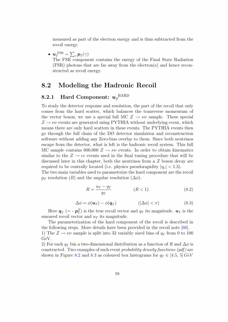
measured as part of the electron energy and is thus subtracted from therecoil energy.
• u FSRT =
∑γ pT (γ)
The FSR component contains the energy of the Final State Radiation(FSR) photons that are far away from the electron(s) and hence recon-structed as recoil energy.
8.2 Modeling the Hadronic Recoil
8.2.1 Hard Component: u HARDT
To study the detector response and resolution, the part of the recoil that onlycomes from the hard scatter, which balances the transverse momentum ofthe vector boson, we use a special full MC Z → νν sample. These specialZ → νν events are generated using PYTHIA without underlying event, whichmeans there are only hard scatters in these events. The PYTHIA events thengo through the full chain of the DØ detector simulation and reconstructionsoftware without adding any Zero-bias overlay to them. Since both neutrinosescape from the detector, what is left is the hadronic recoil system. This fullMC sample contains 600,000 Z → νν events. In order to obtain kinematicssimilar to the Z → ee events used in the final tuning procedure that will bediscussed later in this chapter, both the neutrinos from a Z boson decay arerequired to be centrally located (i.e. physics pseudorapidity |ην | < 1.3).The two main variables used to parameterize the hard component are the recoilpT resolution (R) and the angular resolution (∆φ).
R =uT − qT
qT
(R < 1) (8.2)
∆φ = φ(uT )− φ(qT ) (|∆φ| < π) (8.3)
Here qT (= - pZT ) is the true recoil vector and qT its magnitude. uT is the
smeared recoil vector and uT its magnitude.The parameterization of the hard component of the recoil is described in
the following steps. More details have been provided in the recoil note [60].1) The Z → νν sample is split into 32 variably sized bins of qT from 0 to 100GeV.2) For each qT bin a two-dimensional distribution as a function of R and ∆φ isconstructed. Two examples of such event probability density functions (pdf) areshown in Figure 8.2 and 8.3 as coloured box histograms for qT ∈ [4.5, 5] GeV
98

and qT ∈ [18, 20] GeV bins respectively. From here it is evident that forlow values of qT there is a correlation between R and ∆φ. Moreover thedistributions of R for slices of ∆φ = const are non-gaussian.3)For each qT bin a fit to the pdf observed in the FULL MC sample waspreformed using an ansatz parameterisation:
pdf(x, y) = p0 exp
[−1
2
(x− µ(y)
σx(x, y)
)2]
exp
[−1
2
(y
σy(y)
)2],
where: x ≡ R, y ≡ ∆φ [rad], µ(y) = p1 + p2 · y,
σx(x, y) =
p3, x < µ(y)p4, x > µ(y)
, σy(y) = p5 + p2 · y and
p0 . . . p5 are parameters of the fit.
Effectively only 5 parameters are needed to describe the two-dimensional dis-tribution of R, ∆φ pairs for a given qT bin since p0 is for normalization only.Two such fits are shown in Figures 8.2 and 8.3 as coloured contours forqT ∈ [4.5, 5] GeV and qT ∈ [18, 20] GeV bins respectively.4) A smearing function (f(qT )) is built based on these 32 fits. Hence f(qT )determines the smeared momentum (or uT ) of the boson from its generatorlevel momentum (or qT ) as the input. The smearing of the hadronic responseand resolution (pT and φ) are performed in a single step by f(qT ), inherentlyincluding the correlations between them.
8.2.2 Soft Component: u SOFTT
In the DØ Run I W mass measurement[10], the soft component(underlyingevent and the additional pp interactions) were modeled together by using min-imum bias (MB) events adjusted by a factor that scaled the /ET two-vector ofthese events. This approach, however, is not sufficient for the RunII scenariodue to the much higher instantaneous luminosities and event complexities. InRun II, the underlying event and the interactions of the additional pp pairs,on average, have comparable scalar ET (SET), as shown in figure 8.4. ScalarET of an event is defined as the energy flow in the plane transverse to thebeams. Specifically in the Run IIa Z → e+e− sample, we find 0.9 vertices inaddition to the vertex of the hard scatter, on average. Table 8.1 summarizesthe average scalar ET observed as a function of the number of primary ver-tices reconstructed in a Z event. To deal with the more additional activitycoming from the higher luminosity, we handle the underlying event and theadditional pp interactions by using two separate models, minimum-bias(MB)
99
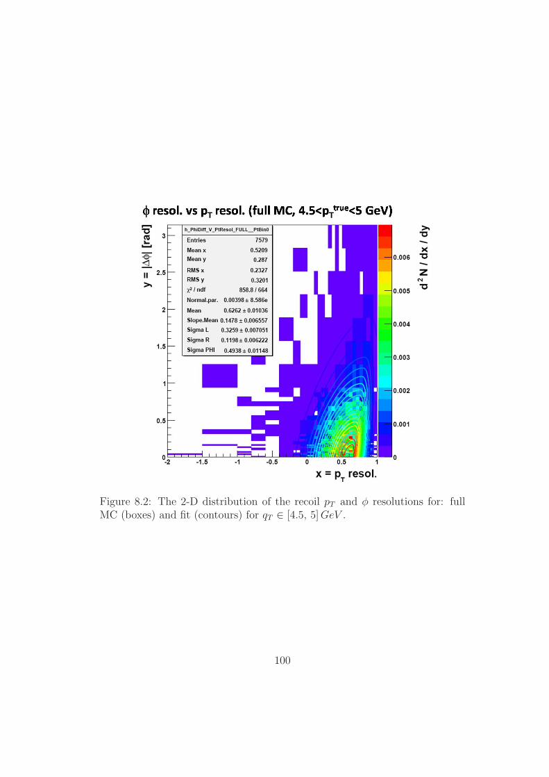
Figure 8.2: The 2-D distribution of the recoil pT and φ resolutions for: fullMC (boxes) and fit (contours) for qT ∈ [4.5, 5] GeV .
100

Figure 8.3: 2-D distribution of the recoil pT and φ resolutions for: full MC(boxes) and fit (contours) for qT ∈ [18, 20] GeV .
101

and zero-bias(ZB) events respectively, as the first step in modeling the softcomponent.
102

Figure 8.4: Underlying event and additional energy contributions to the Zenergy content. The horizontal axis represents the angle δφ between the recoiland the boson. The vertical axis shows the transverse energy flow.
Underlying Event
The underlying event accounts for the interactions between spectator quarks inthe same qq collision that produced the W (Z) boson, which does not dependon the instantaneous luminosity. To model this part,we use the MinimumBias(MB) events with only one reconstructed primary vertex. Minimum biasevents are chosen by a trigger requiring hits in both luminosity counters whichare in time with a beam crossing.
There is no perfect model to describe the underlying event. We need to firstreweight the MB events to match the data. The MB events are reweighted tomake their scalar ET (SET) match the scalar ET of those Z → ee events wherethe electron energy contribution has been removed [60]. The reweighting helpsthe MB events model the underlying event better. The reweighted MB eventinformation is stored in an event library that is used as a lookup table and the/ET of the MB events are used for modeling the underlying event. To improvethe underlying event model, a multiplicative scale factor called αmb is also usedas part of final tuning parameters for the hadronic recoil. αmb is introduced to
103

Table 8.1: Average SET for different numbers of primary vertices in a Z event
Number of primary vertices(excluding vertex of Z)
Mean SET [GeV](excluding electron cones)
0 331 532 743 92
remove any possible double-counting(explained in the next page) and accountfor the difference between the full MC(Z → νν) and the data.
Additional Activity
The additional activity consists of the additional pp interactions that occurin the same or previous beam crossings, detector noise and pileup, etc. The“noise” describes all the sorts of noise in the calorimeter (e.g. from electron-ics, uranium decays, cosmics, beam related backgrounds, etc.). The “pileup”refers to the residual energy in the calorimeter from previous beam crossings.These components are not correlated with the boson pT and do depend on theinstantaneous luminosity.
This part is modeled by using zero-bias(ZB) events. The ZB events weredefined by a trigger requiring only synchronization with the beam crossingclock. The instantaneous luminosity profiles and run number sets of the ZBoverlay have been recorded in the non zero-suppressed1 mode and are used inthe modeling of the recoil to match those of the W (Z) data taking period.
The fact we are using two event information libraries obtained from thedata to model the two sub-components of the “soft” component of the recoilwill cause double counting between the MB and ZB events. Both event li-braries contain the detector noise and soft interactions which do not possessa primary vertex. As mentioned in the above underlying event section, thisdouble counting effect is eliminated by introducing the multipurpose factorαmb for the MB events and tuning αmb to the Z → ee data.
1zero-suppress is a way to suppress energy from the detector noise when recording data.If the signal in one channel is within 1.5 σ around zero after the noise subtraction, the signalwill not be read out. Here, σ is the standard deviation of the noise level.
104

8.2.3 Energy Exchange between Electron and Recoil:u ELEC
T
Since we use a limited cone size to reconstruct the electron energy, some ofthe electron energy outside the reconstruction cone will be calculated into therecoil energy. This is what is called the “electron energy leakage”. On theother hand, as discussed in chapter 7, some of the recoil energy is depositedin the electron reconstruction window(∆u||), which should be subtracted fromthe recoil energy.
8.2.4 Final State Radiation: u FSRT
For final state radiated photons, which are far way from the electron, theirenergies will be included into the hadronic recoil system instead of the electron.
8.3 Over-smearing: Final tuning to the Z → ee
data
As the first step, we have built the hadronic recoil model by dividing it intofour parts. There are correlations between the four parts, along with thedouble-counting we mentioned earlier in this chapter. In simulating the hardcomponent of the recoil, Z → νν full MC events have been used and thereis always some difference between the full MC and data. To account for thecorrelation between the four parts and the difference between the full MCand the data, and also to eliminate the double-counting, we introduce “fine-tuning” or “over-smearing”, in the form of free tunable parameters, to reflectthe differences between our modeled recoil (Z → νν + MB + ZB) and colliderdata.
There are six free parameters, of which three are for the recoil response andthe other three for the recoil resolution. These parameters are determined bycomparing the simulated recoil using the fast MC to collider data for Z → eeevents and will be plugged back into the fast MC to simulate the recoil of theW → eν events.
Figure 8.5 shows the variables of the η and ξ that we are using in deter-mining the tuning parameters[17]. The η axis is defined as the inner bisectorof the angle between the two electrons. The electron direction can be mea-sured very precisely by the tracking system, but the electron energy measuredby the calorimeter could fluctuate due to the calorimeter resolution. So theprojection of the pT of the two electrons onto the η axis only depends on the
105

Figure 8.5: The η − ξ coordinate system in a Z → ee event.
directions of the electrons and is less sensitive to their measured energy. Bydefinition, η imbalance (ηimb) is the sum of these two projections :
ηimb = uT · η + p eeT · η (8.4)
The mean of the ηimb is sensitive to the recoil response and the width ofthe ηimb is sensitive to the recoil resolution. Therefore, the mean and width ofthe ηimb are used to tune the the recoil response and resolution respectively byusing the Z → ee events with a kinematical upper limit of 30 GeV on the recoilpT both in the both data and the fast MC. We make plots of the mean andwidth of the ηimb versus p ee
T . The high p eeT bins are mainly dominated by the
hard component from the initial gluon radiation and hadronization, while thelow p ee
T bins are more affected by the soft component from the initial gluonradiation and hadronization. So by dividing events into different p ee
T bins, wecan gain some extra sensitivity.
8.3.1 Tuning the Hadronic Response
The formula to over-smear the hadronic response RelResp is defined in termsof three tuning parameters named RelScale, RelOffset and τHAD as follows :
RelResp = RelScale + RelOffset · exp−qT
τHAD(8.5)
Here τHAD describes the response of the calorimeter at low values of the recoilmomentum. RelResp is a relative response applied after the hard componentmodeling in section 8.2.1. It greatly affects the mean value of ηimb. qT is the
106

magnitude of the recoil momentum at the generator level. To determine thefine-tuning parameters, templates of the η imbalance distribution with highstatistics are made for the same pZ
T ranges using the fast MC by varying thevalues of the above three parameters. A χ2 is defined by comparing the meanof the ηimb versus p ee
T from the data with that from the fast MC templates.By minimizing the χ2, we found the best fit values are
RelScale = 0.9413 ± 0.0109RelOffset = 1.2016 ± 0.1783τHAD = 3.1758 ± 0.8981 GeV
Figure 8.6 shows the central value and the one standard deviation contourfor the RelScale and RelOffset from the tuning of the hadronic response.Figure 8.7 shows a comparison of the mean of the η imbalance between thedata and fast MC, for the ten different pZ
T bins.
RelScale0.93 0.935 0.94 0.945 0.95
Rel
Off
set
1
1.1
1.2
1.3
1.4 contour for RelScale and RelOffsetσ1
Figure 8.6: Central value and one sigma contour plot for RelScale andRelOffset corresponding to an optimum value of τHAD = 3.1758
8.3.2 Tuning the Hadronic Resolution
The two parameters for the tuning of the hadronic resolution of soft compo-nent in our recoil model are RelSampA and RelSampB. The relative resolutionRelResn is defined as follows :
107

(GeV)eeT
p0 5 10 15 20 25 30
mea
nim
bη
0
2.5
5
7.5
10
Data
FAST MC
(GeV)eeT
p0 5 10 15 20 25 30
χ
-4
-2
0
2
4
Figure 8.7: DATA and FAST MC comparison of the mean of the η imbalancefor the ten different bins in pZ
T .
RelResn = RelSampA +RelSampB√
qT
(8.6)
Here qT is the magnitude of the recoil momentum at the generator level.RelResn is used as a relative resolution smearing applied after the hard compo-nent modeling in section 8.2.1. To tune the resolution of the soft component,the multipurpose scale factor αmb introduced earlier is tuned here. The im-plementation of αmb to tune the soft component is in the same step that hasbeen shown earlier in this chapter as follows :
u SOFTT = − αmb · /ET
MB − αzb · /ETZB (8.7)
The αmb is a free parameter used to adjust the MB events in the softcomponent to help the modeled recoil match the recoil in the data.
The over-smeared hard component by RelSampA and RelSampB and theover-smeared soft component by αmb and αzb are added to predict the finalhadronic recoil pT , which is used to calculate the ηimb in the fast MC to studythe hadronic resolution. Just as the previous tuning for the hadronic response,a χ2 is defined by comparing the width of the ηimb versus p ee
T from the datawith that from the fast MC templates. By minimizing the χ2, we found thebest fit values are
RelSampA = 1.0839 ± 0.0573RelSampB = 0.0αmb = 0.6180 ± 0.0662
108
Here RelSampB = 0.0 without showing the error is because during thefitting we found RelSampB is very consistent with 0 and therefore we fixed itat 0. Figure 8.8 shows the central value and one sigma contour of the αmb
and RelSampA from the tuning of the hadronic resolution. Figure 8.9 shows acomparison of the width of the η imbalance between the data and FAST MC,for the ten different pZ
T bins.
RelSamplingA1.02 1.04 1.06 1.08 1.1 1.12 1.14
mb
α
0.55
0.6
0.65
mbα contour for RelSamplingA and σ1
Figure 8.8: Central value and one sigma contour plot for αmb and RelSampA
corresponding to an optimum value of RelSampB = 0.0
After tuning the free parameters for the response and resolution of therecoil model, we plug the tuned values into the fast MC to combine with theother components (u ELEC
T and u FSRT ) to form the final smeared recoil uT .
8.4 W Mass Uncertainty from the Hadronic
Recoil
To estimate the effect on the W mass from the hadronic recoil, we propagatethe errors of the tuned parameters into the W mass uncertainty. Any imper-fections of the model we built as the first step are transferred into the freeparameters we are tuning. The procedure to determine the W mass uncer-tainty due to the various uncertainties here is by performing fast MC studies[60]. Fast MC W → eν event samples with high statistics are generated byvarying the optimal value of the relevant parameter in steps of its standarddeviation (±1σ, ±2σ). These fast MC samples(“fast MC toy samples”) are
109

(GeV)eeT
p0 5 10 15 20 25 30
wid
thim
bη
0
2.5
5
7.5
10
Data
FAST MC
(GeV)eeT
p0 5 10 15 20 25 30
χ
-4
-2
0
2
4
Figure 8.9: Right: DATA and FAST MC comparison of the width of the ηimbalance for the ten different bins in pZ
T .
fit to the templates (also generated from fast MC with the optimal settings ofthe parameters) to determine the systematic error.
The estimated W mass uncertainty for the three variables(MT , peT and
/ET )are shown in table 8.2.
Table 8.2: Systematic Uncertainties on the W mass obtained for data, due tothe recoil model (for pW
T < 15 GeV).
peT method(MeV) mT method(MeV) pν
T method(MeV)12 6 20
110

Chapter 9
Background
The QCD multi-jet (mostly di-jet) production, W → τν → eννν and Z → eeevents are the major background sources for W → eν events. QCD and Z → eebackground are measured from the real data and the W → τν background isobtained from Geant MC.
9.1 QCD background
Dijet events can pass the W selection cuts if one of the jets mimics an electronand the other is mismeasured. The 2EM and EM+Jet events from colliderdata(see chapter 4) are used for this background study. The number of Wevents is extracted using the matrix method:
N = NW + NQCD (9.1)
Ntrk = εtrkNW + fQCDNQCD (9.2)
where Ntrk and N are the numbers of the W candidate events with and withoutthe track matching requirement, NW is the true number of the real W bosonsand NQCD is the number of QCD events for W candidates without trackmatching requirements. fQCD is the track match fake probability and εtrk isthe track match efficiency, as described below. fQCD and εtrk are measuredusing em+jet and diem events. The track match requirement we used in ouranalysis is the good spatial track matching, which means the matched trackmust have at least one SMT hit and with the track pT > 10 GeV.
Detailed study [62] shows the ηdet and vertex dependence do not affectthe final QCD background shape significantly, even though the fake rate andelectron efficiency are strongly dependent on them. We rely on the kinematicspectrum to measure the W mass. The pT (e) dependence of fQCD and εtrk
111

need to be considered in estimating the QCD background shape and fraction.
9.1.1 fQCD and εtrk
EM+jet events are used to study the fake track match probability. TheseEM+jet events are really dijet events where one of the jets fakes an EM ob-ject. The EM+jets samples are skimmed from RunIIa data with an integratedluminosity of 1 fb−1. We select events by requiring an EM cluster that passesthe EMID requirements and is back-to-back with a jet passing the JET IDrequirements. The fake probability is then the fraction of those EM objectsthat are found to have a matching track. Figure 9.1 shows the pT dependenceof fQCD binned in ηdet. ηdet is binned as (-∞, -1.3), (-1.3, -1.1), ...., (1.1, 1.3),(1.3, +∞).
pT(GeV)30 40 50 60 70 80 90 1000
0.010.020.030.040.050.060.070.080.09
0.1 DetEta region:( -1.1, -0.9)
pT(GeV)30 40 50 60 70 80 90 1000
0.010.020.030.040.050.060.070.080.09
0.1 DetEta region:( -0.9, -0.7)
pT(GeV)30 40 50 60 70 80 90 1000
0.010.020.030.040.050.060.070.080.09
0.1 DetEta region:( -0.7, -0.5)
pT(GeV)30 40 50 60 70 80 90 1000
0.010.020.030.040.050.060.070.080.09
0.1 DetEta region:( -0.5, -0.3)
pT(GeV)30 40 50 60 70 80 90 1000
0.010.020.030.040.050.060.070.080.09
0.1 DetEta region:( -0.3, -0.1)
pT(GeV)30 40 50 60 70 80 90 1000
0.010.020.030.040.050.060.070.080.09
0.1 DetEta region:( -0.1, 0.1)
pT(GeV)30 40 50 60 70 80 90 1000
0.010.020.030.040.050.060.070.080.09
0.1 DetEta region:( 0.1, 0.3)
pT(GeV)30 40 50 60 70 80 90 1000
0.010.020.030.040.050.060.070.080.09
0.1 DetEta region:( 0.3, 0.5)
pT(GeV)30 40 50 60 70 80 90 1000
0.010.020.030.040.050.060.070.080.09
0.1 DetEta region:( 0.5, 0.7)
pT(GeV)30 40 50 60 70 80 90 10000.010.020.030.040.050.060.070.080.09
0.1 DetEta region:( 0.7, 0.9)
pT(GeV)30 40 50 60 70 80 90 10000.010.020.030.040.050.060.070.080.09
0.1 DetEta region:( 0.9, 1.1)
Figure 9.1: fQCD in ηdet bins
Z → ee events from RunIIa are used to study the single electron efficiency.The tag-and-probe method is used [52]. This method was found to bringsome bias based on GEANT MC studies. A 2% uncertainty due to the tag-
112
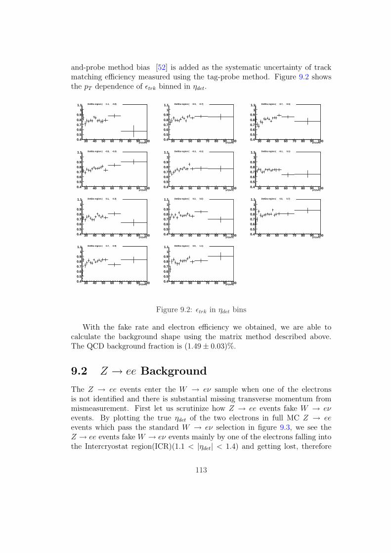
and-probe method bias [52] is added as the systematic uncertainty of trackmatching efficiency measured using the tag-probe method. Figure 9.2 showsthe pT dependence of εtrk binned in ηdet.
pT(GeV)30 40 50 60 70 80 90 1000.4
0.5
0.60.7
0.8
0.91
1.1 DetEta region:( -1.1, -0.9)
pT(GeV)30 40 50 60 70 80 90 1000.4
0.5
0.60.7
0.8
0.91
1.1 DetEta region:( -0.9, -0.7)
pT(GeV)30 40 50 60 70 80 90 1000.4
0.5
0.60.7
0.8
0.91
1.1 DetEta region:( -0.7, -0.5)
pT(GeV)30 40 50 60 70 80 90 1000.4
0.5
0.6
0.7
0.8
0.9
1
1.1 DetEta region:( -0.5, -0.3)
pT(GeV)30 40 50 60 70 80 90 1000.4
0.5
0.6
0.7
0.8
0.9
1
1.1 DetEta region:( -0.3, -0.1)
pT(GeV)30 40 50 60 70 80 90 1000.4
0.5
0.6
0.7
0.8
0.9
1
1.1 DetEta region:( -0.1, 0.1)
pT(GeV)30 40 50 60 70 80 90 1000.4
0.5
0.6
0.7
0.8
0.91
1.1 DetEta region:( 0.1, 0.3)
pT(GeV)30 40 50 60 70 80 90 1000.4
0.5
0.6
0.7
0.8
0.91
1.1 DetEta region:( 0.3, 0.5)
pT(GeV)30 40 50 60 70 80 90 1000.4
0.5
0.6
0.7
0.8
0.91
1.1 DetEta region:( 0.5, 0.7)
pT(GeV)30 40 50 60 70 80 90 1000.4
0.5
0.6
0.7
0.8
0.91
1.1 DetEta region:( 0.7, 0.9)
pT(GeV)30 40 50 60 70 80 90 1000.4
0.5
0.6
0.7
0.8
0.91
1.1 DetEta region:( 0.9, 1.1)
Figure 9.2: εtrk in ηdet bins
With the fake rate and electron efficiency we obtained, we are able tocalculate the background shape using the matrix method described above.The QCD background fraction is (1.49± 0.03)%.
9.2 Z → ee Background
The Z → ee events enter the W → eν sample when one of the electronsis not identified and there is substantial missing transverse momentum frommismeasurement. First let us scrutinize how Z → ee events fake W → eνevents. By plotting the true ηdet of the two electrons in full MC Z → eeevents which pass the standard W → eν selection in figure 9.3, we see theZ → ee events fake W → eν events mainly by one of the electrons falling intothe Intercryostat region(ICR)(1.1 < |ηdet| < 1.4) and getting lost, therefore
113

causing a large missing energy reconstructed. Since our geant simulation is notdoing a good job in describing the real ICR detector, it is certainly necessaryto find another way to estimate the Z → ee Background. We directly extractthe Z → ee events from the real W → eν data.
Figure 9.3: True ηdet of the two electrons in the full MC Z → ee events
The requirements used in selecting Z → ee events out of W → eν data arelisted below.
• Pass standard W → eν selection.
• Require a track with the following properties:
– back to back with the electron
– pT > 25 GeV
– 1.0 < |ηdet| < 1.5
– |z0 − zPV | < 1 cm
114

– opposite charge of the track to the electron
– Scalar sum over pT of all other tracks within a cone of ∆R < 0.4around our track has to be smaller than 4 GeV. Here ∆R is thedistance in η × φ space
– Mass cut: 70 <invariant mass(track, cluster)< 110 GeV
Using this method, the fraction of Z → ee background is found to be(0.80± 0.01)%.
9.3 W → τν Background
The W → τν events, where the τ decays into eνν, could fake the W →eν signal. The electron from τ decay is much softer than the one directlyfrom W decay. Instead of the Jacobian peak at MW /2, the peak appearsat low momenta and falls off rapidly. According to lepton universality, thecross sections of W decays into electrons and τ leptons are the same, butthe τ background is further reduced by the branching ratio of the subsequentτ → eνν decay. Using a detailed simulation of this process, we determine theW → τν → eννν background fraction to be (1.60± 0.02)%.
9.4 Systematics from backgrounds on the W
mass Measurement
The backgrounds from QCD, W → τν and Z → ee are normalized in thesame plot, which is shown in figure 9.4. The W mass uncertainty due toeach background is estimated separately by varying it by ±σ after adding allthe three background to the signal predicted by the fast MC. The results aresummarized in table 9.1. We take the background systematic uncertainties tobe uncorrelated with each other.
115

Fraction Uncertainty Uncertainty UncertaintyMT (MeV) pT (e) (MeV) /ET (MeV)
QCD (1.49±0.03)% 2 4 3Z → ee (0.80±0.01)% 1 2 2W → τν (1.60±0.02)% 1 2 2
Table 9.1: W mass uncertainty due to the QCD, W → τν and Z → eebackgrounds.
(GeV)TM50 60 70 80 90 100 110 1200
50
100
150
200
250
(e) (GeV)T
p25 30 35 40 45 50 55 600
50
100
150
200
250
300
350
400
450
MET (GeV)25 30 35 40 45 50 55 600
100
200
300
400
500
600
700
Figure 9.4: mT , pT (e) and /ET of three different backgrounds with the properrelative normalization. Black: QCD, Red: Z → ee, Blue: W → τν.
116

Chapter 10
Systematic Uncertainties
As discussed separately in the previous chapters, the fast MC is composed ofdifferent parts from different sources, which are parameterized. The param-eters of these different parts have their own uncertainties and therefore havetheir own effects on the W mass uncertainty. To estimate the W mass uncer-tainty due to one specific parameter of the fast MC, we use a large ensembleof pseudo-experiments simulated using the fast MC. A set of high statistics Wmass templates are generated using the fast MC with the default parameters.Pseudo-experiments are performed in a way that a specific parameter is variedindividually ±1σ and ±2σ while keeping all the other parameters unchanged.The pseudo-experiments are fitted using the W mass templates and thereforethe W mass shifts due to the variance of the specific parameter by ±1σ and±2σ are obtained. The W mass change due to the change of the parameteris fit to a line and the slope of the line is used in the usual error propagationformula:
σ2MW
(X) =
(∂MW
∂X
)2
σ2X , (10.1)
where ∂MW
∂Xis the slope and σX is the uncertainty on parameter X. This for-
mula does not include correlations and in many cases we can safely assumethe parameters are nearly uncorrelated. In case there is a strong unavoidablecorrelation, we use the more correct formula which is (here for just two pa-rameters. The extension to three or more parameters can be easily achievedin the same manner.):
σ2MW
(X) =
(∂MW
∂X1
)2
σ2X1
+
(∂MW
∂X2
)2
σ2X2
+ 2σ212
(∂MW
∂X1
)(∂MW
∂X2
)(10.2)
117

where σ12 is the covariance found using the error matrix1.
10.1 Theoretical Uncertainties
The theoretical uncertainties of the W mass measurement are coming fromthe theoretical model we use to generator the events. In chapter 5, we al-ready introduced the event generation and their contribution to the W massuncertainty. Here is the summary.
10.1.1 PDF
The Parton Distribution Functions(PDFs) are derived from fitting experimen-tal results and the uncertainties are propagated to the PDF and then to theW mass measurement. The contribution to the mass uncertainty is 10 MeVfor mT , 11 MeV for pT (e) and 11 MeV for /ET . The systematic error due to thePDF uncertainties is the leading uncertainty from the theoretical descriptionof W boson production.
10.1.2 Boson pT
For the DØ W mass measurement, the uncertainty due to the theoreticaldescription of the transverse momentum spectrum of the boson depend mostsignificantly on the value of g2 in the BLNY parametrization[43] of the non-perturbative region of the spectrum. We use the global fit value of 0.68± 0.02and propagate this uncertainty to the W mass measurement. We find the Wmass uncertainty of 2 MeV when using mT , 5 MeV when using pT (e) and 2MeV for the /ET distribution.
10.1.3 Electroweak Corrections
The dominant electroweak uncertainties come from the final state radiation(FSR).Other electroweak processes, such as ISR, ISR-FSR interference, etc., are stud-ied using WGRAD and ZGRAD programs [50], which are not actually eventgenerators and are used to calculate the cross-sections for these processes. Theelectroweak effect contains the minimum photon energy cut, ISR, ISR-FSR in-terference, photon merge, etc. We find that the uncertainty contribution to
1Error matrix contains information of errors of individual parameters and their corre-lation. The diagonal elements are the square of each parameter error. Other elements arethe covariance of a pair of parameters, which takes into account their correlation.
118

the W mass to be 7 MeV for pT (e), 7 MeV for mT and 9 MeV for the /ET
distribution.
10.2 Experimental Uncertainties
10.2.1 Electron Energy Response
The electron energy response has been tuned using the Z → ee data(Chapter7). Although the individual errors of the scale and the offset are large, thepropagated W mass uncertainty after taking into account of the their highanti-correlation(almost -100%) are greatly reduced. Using this correlation wefind that the systematic uncertainty on the electron energy is 33 MeV,usingmT , pT (e) and /ET . It is the dominant systematic uncertainty for the W massmeasurement and simply limited by the Z → ee statistics.
10.2.2 Electron Energy Resolution
The electron energy resolution is described by three terms: Constant, Sam-pling and Noise(chapter 7). Thanks to the fact we are dealing with electronswith high energy, the noise contribution is negligible. The sampling term wasdetermined using the single electron full MC events. Then the constant termwas determined by forcing the simulated Z in the fast MC to agree with theone measured in the data. So the error of the constant term from the finalstep tuning contains the uncertainty from both the noise and constant terms.The W mass uncertainty from the electron energy resolution is found to besmall and is estimated to be 2 MeV for mT and pT (e) of the electron and 3MeV for /ET .
10.2.3 Electron Energy Non-linearity - Detector Mate-rial Understanding
The non-linearity of the electron energy response is mainly caused by the up-stream material, namely the dead material in front of the calorimeter. Theimpact of the dead material was accounted for by the energy loss correctionapplied to the data(chapter 4). The error of the amount of the dead mate-rial used is propagated into the W mass uncertainty. The uncertainty of theamount of the upstream material results in a W mass uncertainty of 4 MeVmT , 6 MeV pT (e) and 7 MeV for the /ET .
119

10.2.4 Quality of the Electron Energy Loss Corrections
In chapter 7, we discussed the possible bias caused by the different E/ηphys
space of electrons from Z → ee and W → eν events, which we found wasnegligible in the end. Its propagated W mass uncertainty is 4 MeV by usingmT , pT (e) and /ET .
10.2.5 Efficiency
The most influential efficiency for the W mass uncertainty is the u‖ effi-ciency(chapter 6). The u‖ efficiency was fitted with three parameters. Amongthem, what really matters to the W mass measurement is the kink point andthe slope. Their errors along with the correlation are propagated into the Wmass uncertainty. This uncertainty was determined in two steps: First, thedetermination of the efficiency itself from the Z → ee events, and second thescaling of this efficiency to the W events, determined using the DØGeant de-tector simulation. Together the uncertainty is 5 MeV for mT , 6 MeV for pT (e)and 5 MeV for /ET .
10.2.6 Hadronic Recoil
The hadronic recoil is another major source for the W mass uncertainty be-cause it largely affects the determination of /ET and therefore mT (chapter 8).The errors of the parameters for the final tuning of the hadronic recoil arepropagated into the W mass uncertainty due to the recoil. The total uncer-tainty including the hadronic response and resolution is 6 MeV for mT , 12MeV for pT (e) and 20 MeV for /ET .
10.2.7 Background
The systematics from the background(chapter 9) are 2 MeV for mT , 5 MeVfor pT (e) and 4 MeV for /ET . They have a small contribution to the total Wmass uncertainty.
10.3 Summary of the W Mass Uncertainties
The systematic uncertainties due to different sources are summarized in table10.1. First listed are the experimental uncertainties and second are the the-oretical uncertainties, both summed separately. The dominant experimentalsystematic uncertainty is from the electron energy response. Other major con-tributions such as the hadronic recoil and efficiency, etc. are also studied by
120

Source σ(mW ) MeV σ(mW ) MeV σ(mW ) MeVmT pT (e) /ET
ExperimentalElectron Energy Scale 34 34 34Electron Energy Resolution Model 2 2 3Electron Energy Nonlinearity 4 6 7W and Z Electron energy 4 4 4
loss differencesRecoil Model 6 12 20Electron Efficiencies 5 6 5Backgrounds 2 5 4Experimental Total 35 37 41W production anddecay modelPDF 10 11 11QED 7 7 9Boson pT 2 5 2W model Total 12 14 14Total 37 40 43
Table 10.1: Systematic uncertainties on the W mass results.
using the Z → ee events from collider data. So the Z → ee statistics is thelimiting factor in improving the experimental systematics.
121

Chapter 11
Result
11.1 Monte Carlo Closure Test
In previous chapters, the procedure and the various techniques in measuringthe W boson mass have been introduced, some of them in detail. To validatethe whole procedure and the techniques that will be used on data, we per-formed a closure test using the standard DØ full Monte Carlo simulation. Wetreated the full MC sample as collider data to apply the analyzing procedure,including performing the Z boson-based tuning using simulated events.
The differences ∆mW between the fitted W mass and input W massvalue of 80.450 GeV are ∆mW = −0.009 ± 0.015(stat) ± 0.011 ± 0.010 GeV,∆mW = −0.009 ± 0.019(stat) ± 0.007 ± 0.010 GeV and ∆mW = −0.021 ±0.019(stat) ± 0.011 ± 0.010 GeV for the mT , pT (e) and /ET fits respectively.The first uncertainty is from W statistics in the full Monte Carlo sample, thesecond uncertainty is from the statistics of the Z used in the tuning, and thethird uncertainty is due to the residual difference between Z and W in theenergy loss corrections because electrons in the full Monte Carlo sample fromW decay have different energy and η distributions from those from Z decay.
11.2 Result for 1 fb−1 Collider Data
Z → ee events have been largely used as control sample in many aspects of theanalysis, including the data calibration, parameter tuning of the fast MC. Inparticular, Z → ee events were used to calibrate the electron energy responseby forcing the reconstructed Z mass to agree with the world average. So afterall the tuning for the fast MC, it is necessary to check how we have done inpredicting the Z → ee events using the fast MC, especially if the measuredZ mass agrees with with world average as expected. The Z mass fit is shown
122

in figure 11.1. For an input value mZ = 91.188 GeV used in the tuning, thevalue returned from the fit is 91.185± 0.033(stat).
, GeVeem70 75 80 85 90 95 100 105 110
Eve
nts/
0.5
GeV
0
125
250
375
500Data
Fast MC
Fit Region/dof = 153/1602χ
, GeVeem70 75 80 85 90 95 100 105 110
χ
-4
-2
0
2
4
Figure 11.1: The Z mass distribution in data and from the fast simulation(top) and the χ values for each bin (bottom).
Figure 11.2, 11.3 and 11.4 show the distributions of mT , pt(e), /ET with thedata and the fast simulation with the background for the best fit value. Thesefigures also show the bin-by-bin χ values defined as the difference between thedata and the fast simulation divided by the data uncertainty. The potentialstructure in the χ plot in figure 11.4 resides in a region of the distribution thatdoes not carry much mass information.
The measured W mass from the data are shown in table 11.1. One mightwonder why the statistical uncertainty by using the /ET fit is smaller thanthat by using the pT (e) fit since we use the same fit range for both them.The reason is because the average recoil response is not close to 100%, butjust about 60%. So the inferred /ET magnitude is scaled down. Equivalentlywe squeeze more events into the same range for the /ET distribution. This isconfirmed by changing the recoil response to 100% in the fast simulation.
Figure 11.5, 11.6 and 11.7 show the variations of the fitted W mass valuesby changing the lower or higher limit of the fit range.
123

, GeVTm50 60 70 80 90 100
Eve
nts/
0.5
GeV
0
2500
5000
7500
10000
DATAFAST MC
ντW->Z->ee
QCDFit Region/dof = 48/492χ
, GeVTm50 60 70 80 90 100
χ
-4
-2
0
2
4
Figure 11.2: The mT distribution for the data and fast simulation with back-grounds added.
Variable Fit Range (GeV) Result (GeV) χ2/dofmT 65 < mT < 90 80.401± 0.023 48/49
pT (e) 32 < pT (e) < 48 80.400± 0.027 39/31/ET 32 < /ET < 48 80.402± 0.023 32/31
Table 11.1: W mass results from the fits to the data. The uncertainty is onlythe statistical component. The χ2/dof values are computed over the fit range.
124

, GeVeT
p25 30 35 40 45 50 55 60
Eve
nts/
0.5
GeV
0
5000
10000
15000
20000
DATAFAST MC
ντW->Z->ee
QCDFit Region/dof = 39/312χ
, GeVeT
p25 30 35 40 45 50 55 60
χ
-4
-2
0
2
4
Figure 11.3: The pT (e) distribution for the data and fast simulation withbackgrounds added.
125

MET, GeV25 30 35 40 45 50 55 60
Eve
nts/
0.5
GeV
0
5000
10000
15000
20000
DATAFAST MC
ντW->Z->ee
QCDFit Region/dof = 32/312χ
MET, GeV25 30 35 40 45 50 55 60
χ
-4
-2
0
2
4
Figure 11.4: The /ET distribution for the data and fast simulation with back-grounds added.
126

11.3 Combination of Results from Different
Observables
To combine the results from the three observables(mT , pT (e) and /ET ), ensembletests and standard uncertainty propagation methods are used to determine thecorrelation matrix1 which is found to be
ρ =
ρmT mTρmT pT (e) ρmT /ET
ρmT pT (e) ρpT (e)pT (e) ρpT (e) /ET
ρmT /ETρpT (e) /ET
ρ /ET /ET
=
1.0 0.83 0.820.83 1.0 0.680.82 0.68 1.0
,where correlations between the three observables due to statistics, electronenergy response, recoil model and the PDF systematics have been considered.All other sources of systematics (such as QED, backgrounds, efficiencies) havebeen considered as 100% correlated. The results from the three observablesare combined [63] using this correlation matrix. The combined result is
mW = 80.401± 0.021 (stat)± 0.038 (syst) GeV = 80.401± 0.043 GeV.
11.4 Consistency Check
To check the stability of the W mass result, we performed a bunch of consis-tency checks. The basic idea is that we change some aspect of the analysis,especially the parameter on which we model the dependence, to check if westill can obtain consistent result.
A first set of consistency checks has already been presented in the previoussection where we have shown the variation of the measured W mass due tothe change of the fitting range. Here we present additional checks which aredirectly plugged in the middle of the analysis. As mentioned earlier in chapter3, we are essentially measuring the the ratio of the W and Z mass. Whatreally matters is the effect on the measured boson mass ratio by changingsome aspect of this analysis. This means that, whenever we change somethingin the analysis for a consistency check, we should retune the EM energy scaleto the Z. However, we did not do it this way. Instead, we studied the impactof a cut variation or a sample splitting simultaneously in both the data andfast MC to measure the W mass and Z mass separately. Then we check howthe W/Z mass ratio changed.
1The correlation matrix is obtained from the error matrix by dividing each of its elementsby the corresponding pair of parameter errors.
127

Lower window limit (GeV)50 55 60 65 70
(G
eV
)W
M∆
-0.03
-0.02
-0.01
0
0.01
0.02
0.03
Upper limit fixed at 90 GeV - MT
Upper window limit (GeV)80 85 90 95
(G
eV
)W
M∆
-0.06
-0.04
-0.02
0
0.02
0.04
0.06
Lower limit fixed at 65 GeV - MT
Figure 11.5: Sensitivity of the fitted mass values to the choice of fit intervalfor mT distributions when upper edge is fixed (top) and lower edge is fixed(bottom). The yellow regions indicate the expected statistical variations fromsimulation pseudoexperiments. The dashed lines indicate the statistical un-certainty on the mW fit using the default fit range.
128
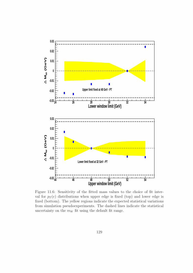
Lower window limit (GeV)24 26 28 30 32 34
(G
eV
)W
M∆
-0.03
-0.02
-0.01
0
0.01
0.02
0.03
Upper limit fixed at 48 GeV - PT
Upper window limit (GeV)44 46 48 50 52 54
(G
eV
)W
M∆
-0.03
-0.02
-0.01
0
0.01
0.02
0.03
Lower limit fixed at 32 GeV - PT
Figure 11.6: Sensitivity of the fitted mass values to the choice of fit inter-val for pT (e) distributions when upper edge is fixed (top) and lower edge isfixed (bottom). The yellow regions indicate the expected statistical variationsfrom simulation pseudoexperiments. The dashed lines indicate the statisticaluncertainty on the mW fit using the default fit range.
129

Lower window limit (GeV)24 26 28 30 32 34
(G
eV
)W
M∆
-0.03
-0.02
-0.01
0
0.01
0.02
0.03
Upper limit fixed at 48 GeV - MET
Upper window limit (GeV)44 46 48 50 52 54
(G
eV
)W
M∆
-0.06
-0.04
-0.02
-0
0.02
0.04
Lower limit fixed at 32 GeV - MET
Figure 11.7: Sensitivity of the fitted mass values to the choice of fit intervalfor /ET distributions when upper edge is fixed (top) and lower edge is fixed(bottom). The yellow regions indicate the expected statistical variations fromsimulation pseudoexperiments. The dashed lines indicate the statistical un-certainty on the mW fit using the default fit range.
130
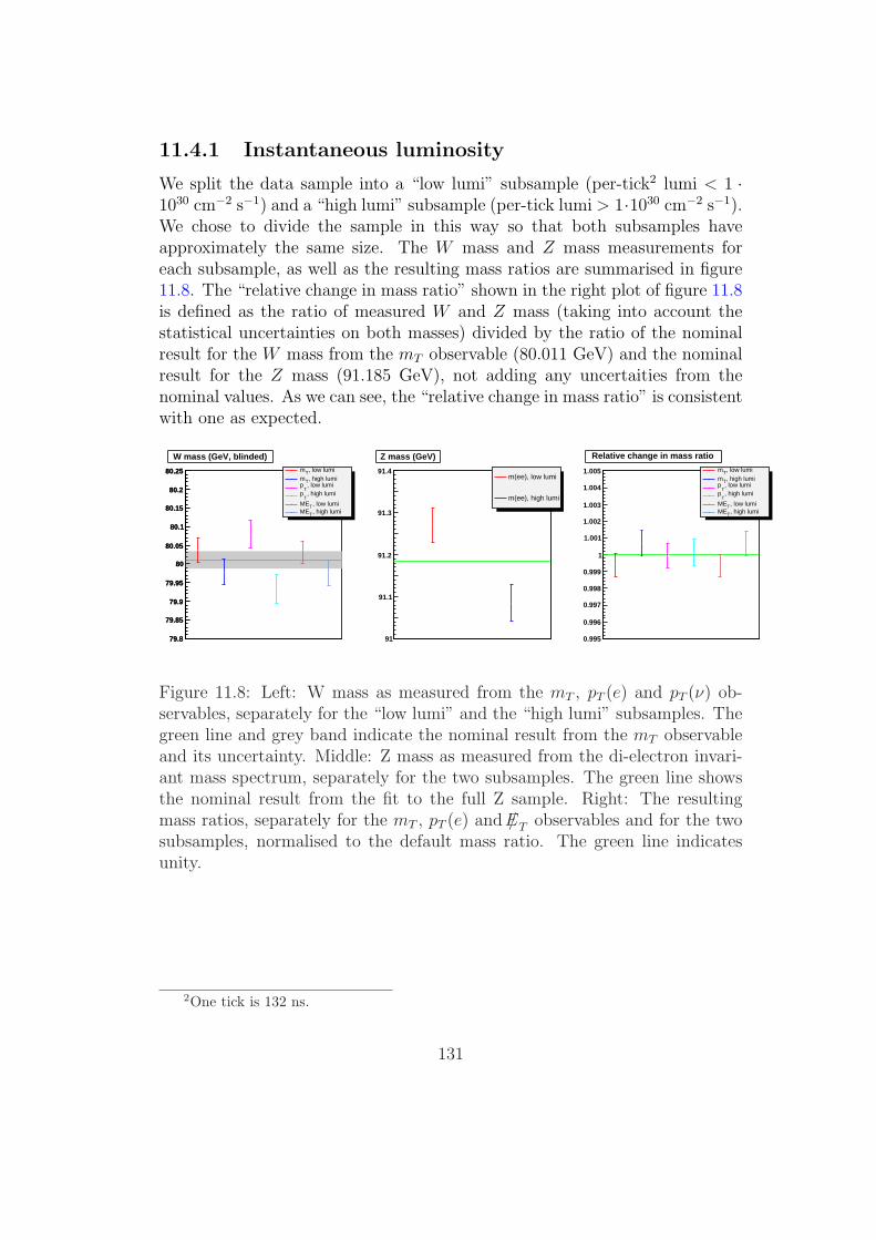
11.4.1 Instantaneous luminosity
We split the data sample into a “low lumi” subsample (per-tick2 lumi < 1 ·1030 cm−2 s−1) and a “high lumi” subsample (per-tick lumi > 1·1030 cm−2 s−1).We chose to divide the sample in this way so that both subsamples haveapproximately the same size. The W mass and Z mass measurements foreach subsample, as well as the resulting mass ratios are summarised in figure11.8. The “relative change in mass ratio” shown in the right plot of figure 11.8is defined as the ratio of measured W and Z mass (taking into account thestatistical uncertainties on both masses) divided by the ratio of the nominalresult for the W mass from the mT observable (80.011 GeV) and the nominalresult for the Z mass (91.185 GeV), not adding any uncertaities from thenominal values. As we can see, the “relative change in mass ratio” is consistentwith one as expected.
79.8
79.85
79.9
79.95
80
80.05
80.1
80.15
80.2
80.25
79.8
79.85
79.9
79.95
80
80.05
80.1
80.15
80.2
80.25 , low lumiTm, high lumiTm, low lumi
Tp
, high lumiT
p
, low lumiTME, high lumiTME
W mass (GeV, blinded)
91
91.1
91.2
91.3
91.4m(ee), low lumi
m(ee), high lumi
Z mass (GeV)
0.995
0.996
0.997
0.998
0.999
1
1.001
1.002
1.003
1.004
1.005 , low lumiTm, high lumiTm, low lumi
Tp
, high lumiT
p
, low lumiTME, high lumiTME
Relative change in mass ratio
Figure 11.8: Left: W mass as measured from the mT , pT (e) and pT (ν) ob-servables, separately for the “low lumi” and the “high lumi” subsamples. Thegreen line and grey band indicate the nominal result from the mT observableand its uncertainty. Middle: Z mass as measured from the di-electron invari-ant mass spectrum, separately for the two subsamples. The green line showsthe nominal result from the fit to the full Z sample. Right: The resultingmass ratios, separately for the mT , pT (e) and /ET observables and for the twosubsamples, normalised to the default mass ratio. The green line indicatesunity.
2One tick is 132 ns.
131

11.4.2 Time
We can also split our data sample into an “early” subsample (before Au-gust 2004) and a “late” subsample (after August 2004). The measured W massand Z mass measurements for each of of the two subsamples, as well as themeasured mass ratios are summarized in figure 11.9. The measured “relativechange in mass ratio” is consistent with one.
79.8
79.85
79.9
79.95
80
80.05
80.1
80.15
80.2
80.25
79.8
79.85
79.9
79.95
80
80.05
80.1
80.15
80.2
80.25 , earlyTm, lateTm, early
Tp
, lateT
p
, earlyTME, lateTME
W mass (GeV, blinded)
91
91.1
91.2
91.3
91.4m(ee), early
m(ee), late
Z mass (GeV)
0.995
0.996
0.997
0.998
0.999
1
1.001
1.002
1.003
1.004
1.005 , earlyTm, lateTm, early
Tp
, lateT
p
, earlyTME, lateTME
Relative change in mass ratio
Figure 11.9: Left: W mass as measured from the mT , pT (e) and pT (ν) ob-servables, separately for the “early” and the “late” subsamples. The greenline and grey band indicate the nominal result from the mT observable and itsuncertainty. Middle: Z mass as measured from the di-electron invariant massspectrum, separately for the two subsamples. The green line shows the nomi-nal result from the fit to the full Z sample. Right: The resulting mass ratios,separately for the mT , pT (e) and /ET observables and for the two subsamples,normalised to the default mass ratio. The green line indicates unity.
11.4.3 Scalar ET(SET)
We now split the data sample into an “low SET” subsample (SET < 50 GeV)and a “high SET” subsample (SET > 50 GeV). The measured W mass andZ mass for each subsample, as well as the resulting mass ratios are summarizedin figure 11.10. Again, the “relative change in mass ratio” is consistent withunity.
132

79.8
79.85
79.9
79.95
80
80.05
80.1
80.15
80.2
80.25
79.8
79.85
79.9
79.95
80
80.05
80.1
80.15
80.2
80.25 , low SETTm, high SETTm, low SET
Tp
, high SETT
p
, low SETTME, high SETTME
W mass (GeV, blinded)
91
91.1
91.2
91.3
91.4m(ee), low SET
m(ee), high SET
Z mass (GeV)
0.995
0.996
0.997
0.998
0.999
1
1.001
1.002
1.003
1.004
1.005 , low SETTm, high SETTm, low SET
Tp
, high SETT
p
, low SETTME, high SETTME
Relative change in mass ratio
Figure 11.10: Left: W mass as measured from the mT , pT (e) and pT (ν) ob-servables, separately for the “low SET” and the “high SET” subsamples. Thegreen line and grey band indicate the nominal result from the mT observableand its uncertainty. Middle: Z mass as measured from the di-electron invari-ant mass spectrum, separately for the two subsamples. The green line showsthe nominal result from the fit to the full Z sample. Right: The resultingmass ratios, separately for the mT , pT (e) and /ET observables and for the twosubsamples, normalised to the default mass ratio. The green line indicatesunity.
11.4.4 Phi fiducial cut
We now vary the phi fiducial requirement. The default requirement, Phi-Mod 3< 0.80, cuts away 10 % of the phase space at each edge of each CCEM mod-ule. We also study two tighter versions of the requirement, namely PhiMod<0.75 and PhiMod< 0.70. The effects of these cut variations are summarizedin figure 11.11. Again, the “relative change in mass ratio” is consistent withunity.
11.4.5 uT cut
We now vary the uT requirement. The default requirement is uT < 15 GeV. Wenow study one tighter version and one more loose version of this requirement,namely uT < 10 GeV and uT < 20 GeV. The effects of these cut variationsare summarized in figure 11.12. Again, the “relative change in mass ratio” isconsistent with unity.
3See section 6.1.
133
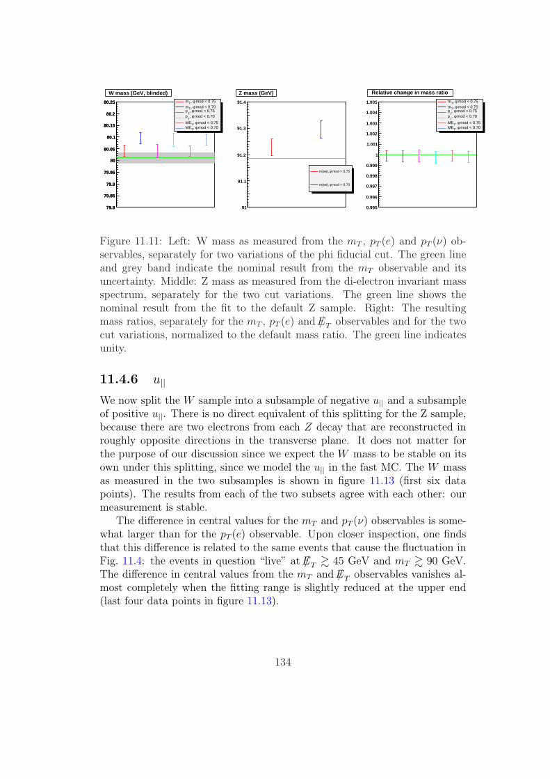
79.8
79.85
79.9
79.95
80
80.05
80.1
80.15
80.2
80.25
79.8
79.85
79.9
79.95
80
80.05
80.1
80.15
80.2
80.25 mod < 0.75φ, Tm mod < 0.70φ, Tm mod < 0.75φ,
Tp
mod < 0.70φ, T
p
mod < 0.75φ, TME mod < 0.70φ, TME
W mass (GeV, blinded)
91
91.1
91.2
91.3
91.4
mod < 0.75φm(ee),
mod < 0.70φm(ee),
Z mass (GeV)
0.995
0.996
0.997
0.998
0.999
1
1.001
1.002
1.003
1.004
1.005 mod < 0.75φ, Tm mod < 0.70φ, Tm mod < 0.75φ,
Tp
mod < 0.70φ, T
p
mod < 0.75φ, TME mod < 0.70φ, TME
Relative change in mass ratio
Figure 11.11: Left: W mass as measured from the mT , pT (e) and pT (ν) ob-servables, separately for two variations of the phi fiducial cut. The green lineand grey band indicate the nominal result from the mT observable and itsuncertainty. Middle: Z mass as measured from the di-electron invariant massspectrum, separately for the two cut variations. The green line shows thenominal result from the fit to the default Z sample. Right: The resultingmass ratios, separately for the mT , pT (e) and /ET observables and for the twocut variations, normalized to the default mass ratio. The green line indicatesunity.
11.4.6 u||We now split the W sample into a subsample of negative u|| and a subsampleof positive u||. There is no direct equivalent of this splitting for the Z sample,because there are two electrons from each Z decay that are reconstructed inroughly opposite directions in the transverse plane. It does not matter forthe purpose of our discussion since we expect the W mass to be stable on itsown under this splitting, since we model the u|| in the fast MC. The W massas measured in the two subsamples is shown in figure 11.13 (first six datapoints). The results from each of the two subsets agree with each other: ourmeasurement is stable.
The difference in central values for the mT and pT (ν) observables is some-what larger than for the pT (e) observable. Upon closer inspection, one findsthat this difference is related to the same events that cause the fluctuation inFig. 11.4: the events in question “live” at /ET & 45 GeV and mT & 90 GeV.The difference in central values from the mT and /ET observables vanishes al-most completely when the fitting range is slightly reduced at the upper end(last four data points in figure 11.13).
134
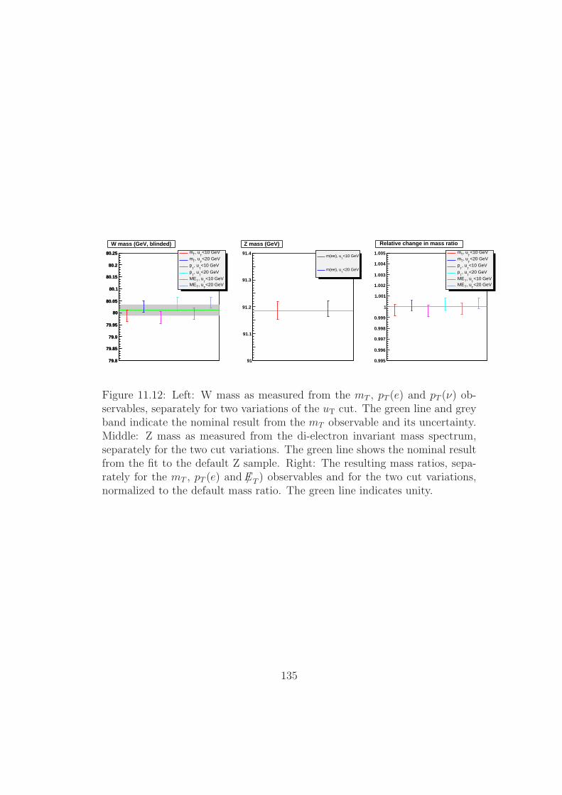
79.8
79.85
79.9
79.95
80
80.05
80.1
80.15
80.2
80.25
79.8
79.85
79.9
79.95
80
80.05
80.1
80.15
80.2
80.25 <10 GeVT
, uTm<20 GeV
T, uTm
<10 GeVT
, uT
p
<20 GeVT
, uT
p<10 GeV
T, uTME
<20 GeVT
, uTME
W mass (GeV, blinded)
91
91.1
91.2
91.3
91.4<10 GeV
Tm(ee), u
<20 GeVT
m(ee), u
Z mass (GeV)
0.995
0.996
0.997
0.998
0.999
1
1.001
1.002
1.003
1.004
1.005 <10 GeVT
, uTm<20 GeV
T, uTm
<10 GeVT
, uT
p
<20 GeVT
, uT
p<10 GeV
T, uTME
<20 GeVT
, uTME
Relative change in mass ratio
Figure 11.12: Left: W mass as measured from the mT , pT (e) and pT (ν) ob-servables, separately for two variations of the uT cut. The green line and greyband indicate the nominal result from the mT observable and its uncertainty.Middle: Z mass as measured from the di-electron invariant mass spectrum,separately for the two cut variations. The green line shows the nominal resultfrom the fit to the default Z sample. Right: The resulting mass ratios, sepa-rately for the mT , pT (e) and /ET ) observables and for the two cut variations,normalized to the default mass ratio. The green line indicates unity.
135

79.8
79.85
79.9
79.95
80
80.05
80.1
80.15
80.2
80.25
79.8
79.85
79.9
79.95
80
80.05
80.1
80.15
80.2
80.25
< 0||
, uTm > 0
||, uTm
< 0||
, uT
p > 0
||, u
Tp
< 0||
, uTME > 0
||, uTME
< 0||
[65,88], uTm > 0
||[65,88], uTm
< 0||
[32,42], uTME > 0
||[32,42], uTME
W mass (GeV, blinded)
Figure 11.13: W mass as measured from the mT , pT (e) and /ET observables,separately for the subsamples of negative and positive u||. For the mT ob-servable, in addition to the results obtained using the nominal fitting range(65− 90 GeV), we also report results from the slightly more restricted fittingrange 65− 88 GeV. Similarly, for the pT (ν) observable additional results fromthe more restricted fitting range 32− 42 GeV are included.
136

Chapter 12
Conclusion and Outlook
12.1 Conclusion
The DØ group has analyzed 1 fb−1 Run II a data, which was collected from2002 to 2006, to measure to W boson mass. We present a precision measure-ment of the mass of the W boson.
MW (mT ) = 80.401± 0.023(stat)± 0.037(syst) GeV (12.1)
MW (pT (e)) = 80.400± 0.027(stat)± 0.040(syst) GeV (12.2)
MW (/ET ) = 80.402± 0.023(stat)± 0.043(syst) GeV (12.3)
The combined result is
mW = 80.401± 0.021 (stat)± 0.038 (syst) GeV = 80.401± 0.043 GeV.
These results are in very good agreement with each other.In the event generation, a W width of 2099.6 MeV was used. It is different
from the value 2093 MeV[64] that has been used for the Tevatron combination.The DØ W mass result is then corrected to[65]
mW = 80.402± 0.043 GeV.
Figure 12.1 shows the results from experiments carried out by the Teva-tron and LEP2. The DØ Run II result agrees well with these experimentand the world average. The DØ measurement is the most precise W bosonmeasurement from one single experiment.
137

(GeV)Wm80 80.2 80.4 80.6
LEP2 average 0.033±80.376
Tevatron 2009 0.031±80.420
D0 Run II 0.043±80.402
D0 Run I 0.083±80.478
Tevatron 2007 0.039±80.432
CDF Run II 0.048±80.413
CDF Run 0/I 0.081±80.436
World average 0.023±80.400
Figure 12.1: W mass measurements at Tevatron and LEP2.
138

12.2 Outlook
From the W mass uncertainty table in the previous chapter, we already men-tioned the dominant experimental systematic is from the electron energy re-sponse, which is simply limited by the Z → ee statistics. Therefore, the easiestway to improve the DØ W mass experimental uncertainty is too increase thesize of the data set. Currently the DØ W mass group has already startedanalyzing the 5 fb−1 Run II data. Assuming the same theoretical uncertainty,we will achieve a W mass uncertainty about 25 MeV. On the other hand,the PDF uncertainty is the dominant one in the theoretical part. With moredata available, the PDF set can also be constrained more precisely. For exam-ple, the W charge asymmetry and jet production measurement will provide apowerful handle on constraining the PDF set.
With the 5 fb−1 DØ result and the 2.3 fb−1 CDF result, we would expecta W mass uncertainty of about 15 MeV for the Tevatron combination.
139

Bibliography
[1] S. Glashow, Nucl. Phys. 22, 579 (1961); S. Weinberg, Phys. Rev. Lett.19, 1264 (1967); A. Salam, Elementary Particle Theory: RelativisticGroups and Analyticity, Nobel Symposium No. 8, edited by N. Svartholm(Almqvist and Wiksell, Stockholm, 1968), p. 367.
[2] D. Griffiths, Introduction to Elementary Particles, John Wiley & SonsInc (1987).
[3] F. Halzen and A. Martin, Quarks and Leptons: An Introductory Coursein Modern Particle Physics,Wiley, 1st edition (1984).
[4] J. Goldstone et al., Phys. Rev. 127: 965 C 970(1962).
[5] Y. Nambu and G. Jona-Lasinio, Phys. Rev. 122, 345-358 (1961).
[6] Y. Nambu and G. Jona-Lasinio,Phys. Rev.124, 246-254 (1961).
[7] M. Peskin and D. Schroeder, An Introduction to Quantum Field The-ory,Westview Press (1995).
[8] L. Ryder, Quantum Field Theory, Cambridge University Press; 2 edition(1996).
[9] A. Sirlin, Phys. Rev. D 22, 971 (1980).
[10] B. Abbott et al. (DØ Collaboration), Phys. Rev. D 58, 092003 (1998).
[11] A. Kotwal and J. Stark, Measurement of the W Boson Mass at the Teva-tron, Annual Review of Nuclear and Particle Science, Nov. 2008.
[12] http://lepewwg.web.cern.ch/LEPEWWG/plots/winter2009/w09 plot mt.pdf
[13] The LEP Electroweak Working Group:http://lepewwg.web.cern.ch/LEPEWWG/plots/winter2009/
140

[14] ALEPH, CDF, DØ DELPHI, L3, OPAL, SLD Collaborations, DØ note5802(2008).
[15] I. Adam, Measurement of the W Boson Mass with the DØ Detector usingthe Electron ET Spectrum, PhD Thesis, Columbia University, New York,New York(1997).
[16] T. Andeen, Ph.D. thesis, Northwestern Unversity, Measurement of theW Boson Mass with the DØ Run II Detector Using the Electron PT
Spectrum(2008).
[17] UA1 Collaboration, G. Arnison et al., Phys. Lett. 122B, 103 (1983);UA2 Collaboration, M. Banner et al., Phys. Lett. 122B, 476 (1983);UA1 Collaboration, G. Arnison et al., Phys. Lett. 126B, 398 (1983);UA2 Collaboration, P. Bagnaia et al., Phys. Lett. 129B, 130 (1983).
[18] M. Syphers, Fermilab Accelerator Division, Accelerator Concepts, Version3.0 (2002).
[19] Fermilab Accelerator Division Document Databases,http://beamdocs.fnal.gov/DocDB//Static/Lists//FullList.html
[20] S. Abachi et al. (DØ Collaboration), The DØ Detector, Nucl. Instr. andMethods, A338, 185 (1994)
[21] DØ Upgrade Collaboration, “DØ Silicon Tracker Technical Design Re-port”, http://www-d0.fnal.gov/trigger/stt/smt/smt tdr.ps.
[22] D. Adams et al. (DØ Collaboration), The D0 Upgrade: Central FiberTracker, Technical Design Report, DØ note 4164(1999).
[23] M. Adams et al. (DØ Collaboration), Central Fiber Tracker TechnicalDesign Report, DØ note 3014(1996).
[24] DØ Collaboration, The DØ Upgrade: Forward Preshower, Muon Systemand Level 2 Trigger, DØ note 2894(1996).
[25] B. Abbott et al. (DØ Collaboration), Measurement of the W boson mass,Phys. Rev. D 58, 092003(1998).
[26] V. Abazov et. al, The Upgraded DØ Detector, Nucl. Instrum. MethodsPhys. Res., A565, 463(2006).
[27] DØ Collaboration, Calorimeter Electronics Upgrade for Run 2, (1998).
141

[28] J. Zhu, Direct Measurement of the W Boson Decay Width in Proton-Antiproton Collisions at
√s = 1.96 TeV, PhD Thesis, University of Mary-
land, College Park, Maryland (2004).
[29] Particle Data Group, Phys. Lett. B, Vol. 667(2008).
[30] F. James, Minuit: A system for Function Minimization and Analysis ofParameters Errors and Correlations, M. Roos Comput. Phys. Commun.10, 343 (1975).
[31] DØ W mass group, Measurement of the W boson mass using Run IIadata, DØ note 5868, (2009).
[32] P. Petroff and J. Stark, Proposal to perform a blind measurement of theW mass in Run II, DØ note 5388(2007).
[33] T. Golling, Measurement of the tt Production Cross-Section at√
s =1.96 TeV in the Muon+Jets Final State using a Topological Method, DØnote 4667(2005).
[34] D. Adams, Finding Tracks, DØ note 2958(1996).
[35] H. Greenlee, The DØ Kalman Track Fit, DØ note 4303(2004).
[36] A. Schwartzman and M. Narain, Vertex Fitting by means of the KalmanFilter techinque , DØ note 3907(2001).
[37] G. Steinbruck, Measurement of the Angular Distribution of Electronsfrom W Boson Decay at DØ PhD Thesis, University of Oklahoma (1999).
[38] R. Wigmans, Calorimetry, Oxford University Press (2000).
[39] P. Nadolsky, Theory of W and Z boson production, ANL-HEP-CP-04-138,(2004).
[40] E. Mirkes, J. Ohnemus, W and Z polarization effects in hadronic collisions,Physical Review D, 50, 5692, (1994).
[41] C. Balazs and C.P. Yuan, Soft gluon effects on lepton pairs at hadroncolliders, Phys. Rev. D 56, 5558 (1997).
[42] J. Collins, D. Soper and G. Sterman. Nucl. Phys. B250(1985) 199.
[43] F. Landry, R.Brock, P. Nadosky, C.P. Yuan, Fermilab Tevatron run-1 Zboson data and the Collins-Soper-Sterman resummation formalism, Phys.Rev. D 67, 073016 (2003).
142

[44] H.L. Lai et al., Phys. Rev. D 55, 1280 (1997); J. Pumplin et al., JHEP0310, 046 (2003).
[45] J. Guo, J. Zhu, J. Hobbs and R. Mccarthy, PDF Uncertainty for W massMeasurement, DØ note 5078(2006).
[46] T. Aaltonen et al. (CDF Collaboration), Phys. Rev. Lett. 99, 151801(2007); T. Aaltonen et al. (CDF Collaboration), Phys. Rev. D 77, 112001(2008).
[47] J. Osta, Combination of the Run IIa W boson mass measurements, DØnote 5913(2009).
[48] E. Barbiero and Z. Was, Comp. Phys. Commun. 79, 291 (1994).
[49] J. Guo, J. Zhu, J. Hobbs and R. Mccarthy, Electroweak Uncertainty forthe W Mass Measurement, DØ note 5666(2008).
[50] U. Baur, S. Keller and D. Wackeroth, Phys. Rev. D 59 013002 (1999).
[51] U. Baur, S. Keller and D. Wackeroth, A Monte Carlo pro-gram for the calculation of electroweak radiative correc-tions to Z boson production at hadron colliders, Available athttp://ubhex.physics.buffalo.edu/∼baur/zgrad2.tar.gz
[52] J.Hays, J.Mitrevske,C.Schwanenberger,T.Toole, Single Electron Efficien-cies in p17 Data and Monte-Carlo Using p18.05.00 d0correct, DØ note5105(2006)
[53] Talk given by H. Schellman and D. Chapin, W/Z toelectrons weekly meeting, March 23, 2004 (http://www-d0.hef.kun.nl//fullAgenda.php?ida=a0429&fid=61).
[54] Talk given by J. Stark, W mass meeting, May 23, 2007 (http://www-d0.hef.kun.nl//askArchive.php?base=agenda&categ=a07740&id=a07740s1t0/transparencies).
[55] Tim Andeen, Feng Guo, Jun Guo and Junjie Zhu, Effect of Recoil onElectron Identification Efficiency, DØ note 5686(2009).
[56] “Studies of energies below electron window for W mass measurement”,F. Guo, J. Hobbs, R. Mccarthy, P. Petroff, M. Rijssenbeek, J. Stark,J.Zhu, DØ Note 5661(2008).
143
[57] Tim Andeen and Alex Melnitchouk, Measurement of Electron EnergyScale and Offset with Z → ee Full Monte Carlo and Data, DØ Note5662(2009)
[58] C. Fabjan and F. Gianotti, Calorimetry for particla physics, Rev. Mod.Phys., Vol.75 (2003).
[59] A. Melnitchouk, M. Wetstein, Determination of the constant term of theelectron resolution, DØ Note 5879(2009).
[60] T. Andeen, M. Cwiok, J. Guo, J. Hobbs, J. Osta, J. Stark, J. Zhu, Model-ing the Hadronic Recoil for the W Mass Measurement in Run IIa (MethodI), DØ Note 5668 (2008).
[61] Philip R. Bevington Data Reduction and Error Analysis for the PhysicalSciences, Mc-Graw Hill Inc.
[62] J. Guo, J. Zhu, J. Hobbs and R. Mccarthy, Background for W MassMeasurement, DØ note 5665(2008).
[63] L. Lyons, D. Gibout, and P. Clifford, Nucl. Instrum. Methods in Phys.Res. A 270, 110 (1988).
[64] The Tevatron Electroweak Working Group, Combination of CDF and DØResults on W Boson Mass and Width, FERMILAB-TM-2415 1st August2008
[65] DØ W mass group, Combination of CDF and DØ Results on the W BosonMass, DØ note 5938(2009).
144