Vol.:(0123456789)

SN Computer Science (2021) 2:473 https://doi.org/10.1007/s42979-021-00854-8

SN Computer Science

ORIGINAL RESEARCH

A Predictive Resource Allocation for Wireless Communications Systems

Márcio J. Teixeira1  · Varese S. Timóteo1

Received: 19 November 2020 / Accepted: 6 September 2021 / Published online: 27 September 2021 © The Author(s), under exclusive licence to Springer Nature Singapore Pte Ltd 2021

AbstractUsing event-driven computer simulations, we test a predictive resource allocation scheme for broadband wireless commu-nications systems based on the Kalman Filter. We implemented the filter in six different scheduling algorithms and selected the best performing of them (EXP Rule and FLS) for a detailed analysis. We considered several simulation scenarios with velocities ranging from 0 to 350 km/h representing pedestrian, vehicular and high-speed train scenarios. We also considered different traffic profiles by changing the number of mobile devices between 10 and 250. Our simulations showed improve-ment in throughput, spectral efficiency, and a decrease in packet loss rates for two schedulers: the EXP Rule and the Frame Level Scheduler. Our predictor can be applied to any wireless system that performs centralized resource allocation based on data rate or any other quantity that needs to be estimated for resource distribution in a network.

Keywords Resource allocation · Mobile networks · Predictive scheduler · Event-driven simulation

Introduction

Historical Background and Motivation

Mobile communication systems changed dramatically the traffic paradigm since their appearance in the late 1970s both in volume and profile. With 2G systems traffic was circuit-switched and network planning based on the availability of voice channels. For this reason, design was focused on the blocking probability of the voice channels because data demand was very incipient. The change to 3G systems intro-duced dedicated traffic channels for data sessions and the dimensioning process required to take the data traffic profile

into account. The arrival of 3.5G made for the first time possible to users have mobile applications with an accept-able Quality of Service (QoS) and this feature increased the usage of video, Voice over IP (VoIP), and other multimedia services through cellular network together with the massive adoption of social media in the decade of 2010.

Available bandwidth in mobile networks, which was already a problem for data transmissions, became criti-cal with most of the subscribers requesting more radio resources for their video and data applications. Ericsson mobility report forecasts that the 4G long-term evolution (LTE) networks will remain the most used access technology until 2026 after reaching a peak of 4.5 billion subscribers in 2021 while 5G is expected to approach 3.5 billion users mostly in early adopters such as North America and Western Europe. This will increase mobile traffic from the current 51 EB/month to 226 EB/month. Around 97 % of this volume will come from smartphones carrying an average of 34 GB/month (nowadays this traffic is close to 9.5 GB/month) [1].

The Covid-19 pandemics shifted the traffic locations from offices and public places to homes and this change was driven mostly by virtual working environments, usage of applications for food and goods delivery, and entertain-ment (e.g. streaming and gaming). Optimization of network resources is critical to ensure QoS and, regardless of the access technology, spectrum will always be a limited and disputed resource. Therefore, efficient schedulers performing

This work was supported by the Coordenação de Aperfeiçoamento de Pessoal de Nível Superior - CAPES, Finance Code 001 (MJT), Fundação de Amparo à Pesquisa do Estado de São Paulo - FAPESP, grant 2019/010889-1 (VST), Fundo de Apoio ao Ensino, à Pesquisa e à Extensão - FAEPEX, grant 3258/19 (VST) and Conselho Nacional de Desenvolvimento Científico e Tecnológico - CNPq, grant 306615/2018-5 (VST).

* Márcio J. Teixeira mjteixeira@gmail.com

Varese S. Timóteo varese@unicamp.br

1 Grupo de Óptica e Modelagem Numérica - GOMNI, Faculdade de Tecnologia - FT, Universidade Estadual de Campinas - UNICAMP, Limeira, SP, Brazil

SN Computer Science (2021) 2:473473 Page 2 of 15

SN Computer Science

resource allocation (RA) in mobile networks are of key importance. References [2, 3] reviewed developments of downlink and uplink schedulers in LTE Networks.

Some Developments on Resource Allocation and Contribution of This Work

In cellular networks, media access control (MAC) layer is responsible for RA and scheduling is performed at Evolved NodeB (eNodeB) in LTE and at Next Generation Node B (gNB) in 5G networks. Depending on objective and net-work constraints schedulers may engage at every transmis-sion time interval (TTI) or multiples of these intervals. Fre-quent triggering of the scheduling algorithm has a two-fold effect: on one side it allows a better distribution of network resources at the cost of extra signaling between the radio access nodes [4].

One of the goals of an efficient scheduler is to maximize aggregated network throughput and spectrum efficiency. To maintain quality in video calls and transmissions packet loss ratio (PLR) should also be kept low. For delay-sensitive applications, it is expected that it can handle User Equip-ment (UE) requests and remain within the maximum delay allowed by applications. Fairness is also an important feature and, in general, these goals are not achieved simultaneously and one must make a few compromises when designing a new scheduler. There are various solutions in literature with different approaches and results. Below we list a few of them. In [5] authors explained that increased throughput does not necessarily mean quality as it also increases the average PLR. They proposed a cross-layer design for the scheduler combining information on throughput, application QoS and fairness that dynamically allocate resources and optimize system parameters such as modulation and coding scheme (MCS) adapting channel quality at each resource block. Following this cross-layer paradigm, the work of [6] blended objective measurements with a mean opinion score experience of users providing a scheduler whose perfor-mance is also tied to quality of experience (QoE). Separating real-time from non-real-time traffic aiming to balance data delivery is also a common strategy for RA as exemplified in [7] where authors proposed a change in the maximum-largest weighted delay first (M-LWDF) scheduler. Solving a minimization or a maximization problem (e.g. get the maxi-mum rate per user) is another common approach to design schedulers. However, some of them are NP-hard problems and can only be solved by heuristic methods [8, 9]. All the works exemplified above use the non-predictive approach meaning that there is no dynamic scheme to change prede-fined parameters in schedulers.

Conversely, predictive schedulers forecast values of a given measured quantity or a performance indicator to maximize the allocation of resources. The work of [10]

used neural networks consisting of long–short term mem-ory (LSTM) using Keras and TensorFlow as back-end and predicted traffic patterns for one week with good accuracy. An interesting possibility, in this case applied to machine-to-machine (M2M) communications, appeared in [11] where they used the concept of directed information (DI) to cal-culate the correlation between four devices to predict traffic based on entropy and mutual information. The work of [12] proposed a guided search algorithm as an alternative low-complexity solution. The solution of this guided search is highly dependent on the variance of signal measurements over time: a super estimated variance can allocate excessive airtime to users while underestimated variance would sub allocate resources. These authors used the Kalman Filter (KF) to predict these variances and adaptively configure the guided search algorithm to optimal values. Their results were verified with an open-source simulator and a commer-cial optimization solver and they reported that the proposed solution runs in less than one millisecond but this study is restricted for a maximum of 12 users moving at 60 km/h.

The contribution of our work is to use a simple, real-time predictor based in the Kalman Filter that improves through-put and spectrum efficiency and reduces packet loss. This approach does not rely on historical data or training of neural networks; it predicts the rate R̄ every TTI instead of using a blind equal throughput formula, Eq. (12). When we increase the number of users disputing network resources the filter effect is more noticeable as we will show in following sec-tions. The drawback is that the predictor compromise fair-ness of resource distribution among users.

This work is organized as follows: In Sect. 2 we briefly describe the Kalman filter (2.1), the RA process in mobile systems (2.2), six selected schedulers and their metrics (2.3) and finally how we use the filter to improve these metrics (2.4). Section 3 compares the values of throughput, packet loss rates and delay with and without the predictor when we increase the number of users and velocity of mobiles. Then we selected the best performing schedulers in this test (the FLS and EXP Rule) and proceeded to extended simulations (Sect. 4) where the number of users (and consequently the network traffic) was extended to 250 mobiles. We studied the effect of the predictor in throughput (4.1), packet loss (4.2) and added to our study spectral efficiency (4.3) and fairness index (4.4). Finally, Sect. 5 discusses results and outlines future extensions of this work.

SN Computer Science (2021) 2:473 Page 3 of 15 473

SN Computer Science

Resource Allocation with the Kalman Filter

Short Description of the Kalman Filter

As it is well-known the KF [13] has two steps: prediction and correction. For given initial estimates of x̂k−1 and Pk−1 , the prediction steps calculate the values of x̂−

k and P−

k the

projected error covariance (see for example [14]) :

with A as a matrix that relates the state at the previous time step k − 1 to the state at the current step. The superscript minus sign mean that it is a a priori value of given state x and the circumflex that it is an estimated quantity. So is x̂−

k

the a priori estimate of state x. The correction step is given by the following equations:

where � represents the identity matrix. During the cycle of prediction and correction, we calculate the Kalman gain Kk using the new estimates for x̂k and Pk . At the end of the loop k is incremented by 1, the values of x̂−

k and P−

k are updated

and the cycle restarts. Similarly to A, the matrix H will relate the state of the system X to the measurement z by the relation zk = Hxk +R . The quantities Q and R are the process and measurement noise covariance respectively that may or may not change at every step of the simulation [14].

Resource Allocation

The resource scheduler is the logical entity in the eNodeB or gNB that assigns for a given user enough bandwidth in downlink and uplink to match QoS requirements of their applications. With distinct requirements on jitter, throughput, delay and packet loss, the role of the scheduler is to maintain the guaranteed QoS of applications regardless of the uncer-tainties of radio environment [15]. LTE uses the orthogonal frequency division multiple access (OFDMA) as modulation technique meaning that a UE has resources assigned both in the time domain (symbols) as well as in frequency domain (sub-carriers). One LTE frame is composed of ten subframes of 1 ms each that are subdivided into time slots of 0.5 ms. Together these subframes in the time domain and 12 sub-carriers of 15 kHz (180 kHz) in the frequency domain build a Resource Block (RB), the smallest resource unit assigned to

(1)x̂−k=A x̂k−1 ,

(2)P−k=A Pk−1 A

T + Q ,

(3)Kk= P

−kH

T (H P−kH

T +R)−1 ,

(4)x̂k= x̂

−k

+ Kk(z

k− H x̂

−k) ,

(5)Pk= (� − K

kH) P−

k,

a user within an LTE frame. Resource scheduler will allocate the RBs based on UEs requests and the number of available blocks will depend on the bandwidth assigned to LTE. For 1.5 MHz only six RB are assignable, for 5 MHz there will be 25 RBs going up to 100 RBs when operator has 20 MHz of available spectrum [16]. Every application session started in the network is called a flow and the goal of the scheduler is to give the right amount of RBs to users to maintain the QoS of their flows. The output of the scheduler algorithm is a number mi,j called metric. So, given a flow i with a given RB j, the metric is the priority that a scheduler will allocate the RB j for a flow i, that is, the bigger the metrics the stronger the priority of allocation to a RB [2].

To have an efficient scheduler handling real time traffic a few basic requirements must be fulfilled. The first is computa-tional simplicity specially if they work within the time window of one TTI, i.e.,1 ms. As the usage of networks increase scal-ability is important because calculations will raise by a factor of N ×M per TTI [2] with N representing the number of users and M the available RBs. Finally, it is desirable to distribute RBs equally among users, that is, fairness. Achieving these goals simultaneously may not be an easy task.

There is no requirement in 3GPP standards for a specific type of scheduler so we can, in principle, pick anyone. We ruled out the popular Round Robin scheduler because its per-formance gets worse in mobile environments compared to the Proportional Fair (PF) as shown in [17]. Therefore, we selected six schedulers that make use of channel aware strate-gies aiming to maximize throughput by measurements of the quality perceived by users. Except for the simplest of them, the Proportional Fair, all make use of QoS aware strategies that are based on maximum delay and allowed packet loss. Some schedulers require a predefined maximum allowed packet loss per user. When this is the case, we set �i = 1%.

Schedulers and Metrics

Proportional Fair

This scheduler favors the users with smaller data rates in past periods. The proportional fair scheduler metric �i,j is propor-tional to the inverse of past data rates and is defined by:

where R̄i(t − 1) is the estimate of the i-th flow in previous TTI and di

j(t) is the data rate of i-th flow at the j-th RB.

M‑LWDF

This scheduler uses a bounded delay, i.e., it will differentiate the real-time versus non-real-time traffic. Treating the former with the PF metric, Eq. (6), and the later by:

(6)𝜔i,j = d ij(t) ∕ R̄i(t − 1) ,

SN Computer Science (2021) 2:473473 Page 4 of 15

SN Computer Science

It considers the Head of Line packet (HOL) delay DHOL,i multiplied by a factor �i = − log �i∕�i , being �i the accept-able PLR for user i and �i the delay threshold for that user.

Exponential Rule/Proportional Fair (EXP/PF)

As its name says it combines two parts: an exponential function End-to-End (E2E) delay and the PF metric for non-real-time flows. The metrics is given by:

where � is defined as:

and 1∕Nrt is the active number of downlink real-time flows.

LOG Rule

The LOG rule scheduler is very similar to the EXP Rule. It is given by:

with a = 5∕�i , b = 1 and c = 1.1 according to Ref. [2].

EXP Rule

EXP Rule has a similar metric of the one shown in Eq. (8) and it is given by the generic expression:

In our simulations we use ai = 6∕�i , b = c = 1 as in Ref. [18]. The term under the square root is the average delay of the HOL.

The Frame Level Scheduler (FLS)

This scheduler was designed to handle real-time multime-dia services in LTE networks and has an upper level that analyses the needs of transmission flows at the beginning of each LTE frame. The design of the upper layer was

(7)mM-LWDFi,j

= �i DHOL,i ⋅ �i,j .

(8)mEXP/PFi,j

= exp

��i DHOL,i − �

1 +√�

�⋅ di

k(t) ⋅ �i,j ,

(9)� =1

Nrt

Nrt∑i=1

�i DHOL,i ,

(10)mLOGi,j

= bi log(c + ai DHOL,i) ⋅ �i,j ,

(11)mEXPi,j

= bi exp

⎛⎜⎜⎜⎝

ai DHOL,i

c +�

(1∕Nrt)∑

j ai DHOL,j

⎞⎟⎟⎟⎠⋅ �i,j .

based on control theory and at the lower layer a PF algo-rithm is chosen to handle the non-real-time flows. Despite its implementation complexity, the scheduler handles well video and multimedia traffic. There is no closed-form for a metric mi,j in this scheduler, and details of its design are explained in [19].

Using the KF to Predict Traffic Flows

As seen in Sec. 2.3 all schedulers, except the FLS, will make explicit use of the proportional fair metric, Eq. (6), to handle real-time flows. The denominator of �i,j is estimated every TTI for each user [2] so that:

with k being the time-stamp and � = 0.8 as used in ref. [18].Our contribution is to improve the estimate of R̄k using a

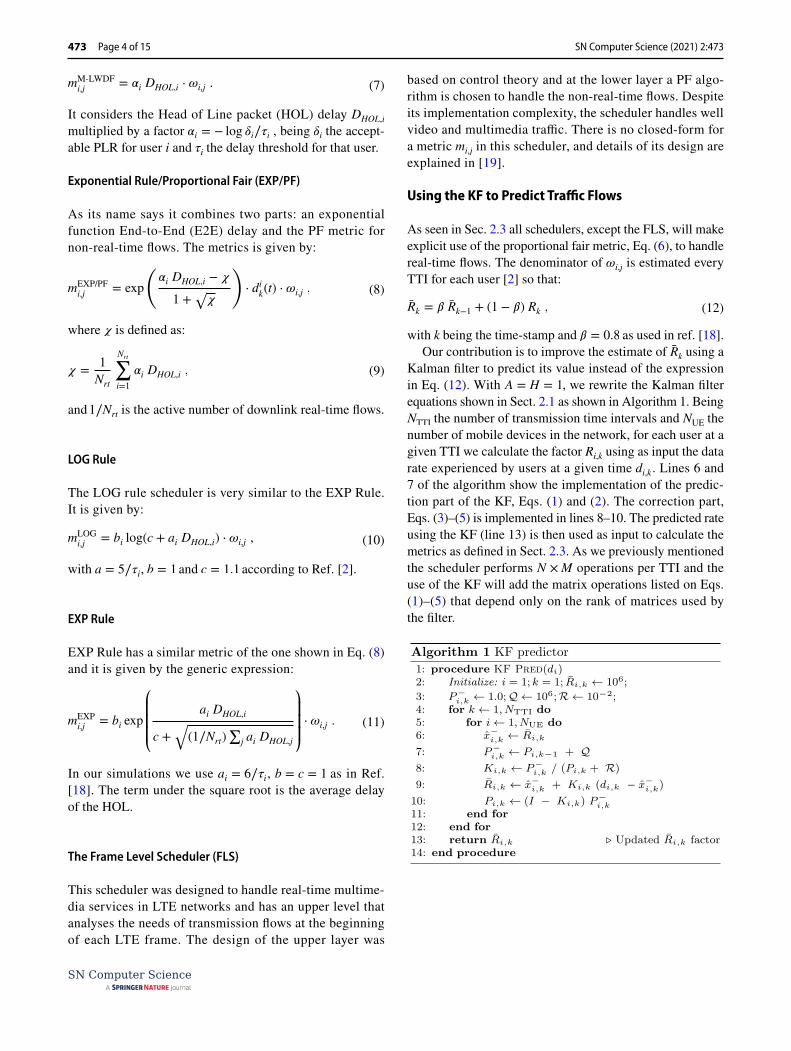
Kalman filter to predict its value instead of the expression in Eq. (12). With A = H = 1 , we rewrite the Kalman filter equations shown in Sect. 2.1 as shown in Algorithm 1. Being NTTI the number of transmission time intervals and NUE the number of mobile devices in the network, for each user at a given TTI we calculate the factor Ri,k using as input the data rate experienced by users at a given time di,k . Lines 6 and 7 of the algorithm show the implementation of the predic-tion part of the KF, Eqs. (1) and (2). The correction part, Eqs. (3)–(5) is implemented in lines 8–10. The predicted rate using the KF (line 13) is then used as input to calculate the metrics as defined in Sect. 2.3. As we previously mentioned the scheduler performs N ×M operations per TTI and the use of the KF will add the matrix operations listed on Eqs. (1)–(5) that depend only on the rank of matrices used by the filter.

(12)R̄k = 𝛽 R̄k−1 + (1 − 𝛽) Rk ,

SN Computer Science (2021) 2:473 Page 5 of 15 473

SN Computer Science

Effects of KF Predictor in the Schedulers

In this section, we perform a systematic analysis of the use of Kalman filter to predict R̄k in the schedulers and compare it with the usual expression for given by Eq. (12). For this study, we used LTE-Sim [18] a flexible open-source simu-lator coded in C++ that allows various configurations such as radio propagation models (urban, suburban, and rural), movement pattern (random or fixed direction), number of UEs, number of cells, available bandwidth, effective cell radius among others. When a simulation ends, the output is a list of events with a timestamp, type of traffic, bearer (i.e. application per user), packet size in bytes and delays that are post-processed to get the performance indicators. Simulated scenarios consisted of variations in the number of UEs, mobile velocity, and maximum delay for both selected schedulers. To ensure accuracy, each scenario is simulated 10 times, and the values of performance indicators are aver-aged. The parameters used for this simulation are shown in Table 1.

Dependence on the Number of UEs

Our previous work [20] implemented the KF in the resource allocation routine of LTE-Sim and studied some perfor-mance indicators for 6 schedulers (PF, M-LWDF, EXP, FLS, EXP Rule and LOG Rule) and two mobility scenarios: pedestrian with v = 3 km/h and vehicular with v = 120 km/h and 10, 20, 30 and 40 UEs. Data in Fig. 1 use an intermedi-ate value of v = 90 km/h to assess performance of the sched-ulers with respect to increasing number of UEs.

We obtained, as expected, a similar result as our previ-ous study [20]. The throughput increases for FLS and EXP

Rule is observed when we introduce the filter, and the effect gets more noticeable as the number of UEs increment in the network. This can be observed by comparing the left (without prediction) and right (with prediction) top panels of Fig. 1. We also observe a significant decrease in the packet loss rate when we compare the two bottom panels of Fig. 1, which display the results with (right) and without (left) the KF based predictor.

Dependence on the Velocity

From Fig. 2 we see that both throughput and PLR have a relatively small variation with the change in velocity, which validates our choice of Sect. 3.1 to use v = 90 km/h . We see similarities with Fig. 1 when we apply the KF, i.e., perfor-mance of FLS and EXP Rule improve significantly com-pared to other schedulers.

Best results happen for the EXP Rule that shows an improvement of about two times in throughput (see green lines in the top panels of Fig. 2) and a reduction from ∼ 12 to ∼ 4% in the packet loss rate (see green lines in the bot-tom panels of Fig. 2). This shows that the performance of the EXP Rule scheduler with the predictor approaches the performance of the FLS scheduler which is particularly designed for handling real-time multimedia traffic [19]. The improvement of more than 35 % in throughput for M-LWDF although significant in relative numbers is no match for the absolute values achieved by FLS or the EXP Rule schedul-ers. The same applies to other schedulers that do not benefit from KF sometimes even having its performance degraded, for example the PF.

Effects on the Delay

Some schedulers such as the EXP and LOG rule take the maximum allowed application delay in their metrics as we mentioned in Sect. 2.3. This is important because some applications have strict requirements on maximum permit-ted delay. In this paper, we used two different values for the target delay: 0.04 s and 0.1 s. The simulated measurements of delay when we introduce the KF schedulers are compiled in Fig. 3. First thing to notice is that PF scheduler fails to remain within required delay. (note that we scaled down the values by a factor of 10 for better visualization). This is expected because the simplicity of the PF metric is not suited for handling real or near real-time flows. For remain-ing schedulers, addition of filter does not help to reduce delay. As all of them remain in the region well below the target delay we can say that these schedulers are “delay neu-tral” with respect to the use of the predictor.

Before proceeding, we summarize our findings on the use of the Kalman filter to predict R̄k :

Table 1 Simulation parameters

Parameter Value

Bandwidth (MHz) 5.0Resource blocks 25Number of TTI 1000Cell radius(km) 0.5Number of UEs 10, 20, 30, 40Moving pattern Random directionApplications Video, VoIP and CBRVideo bit rate (kbps) 128Velocities (km/h) 0, 3, 6, 10, 15, 20, 25,

30, 60, 90, 120, 150, 200,250, 300 and 350

Maximum delay (ms) 0.1 and 0.04Schedulers M-LWDF, EXP, FLS,

EXP Rule, LOG rule, PF

SN Computer Science (2021) 2:473473 Page 6 of 15

SN Computer Science

(i) the use of KF shows better performance for an increasing number of UEs in accordance to our pre-vious work [20],

(ii) velocity has little influence in schedulers throughput, PLR and delay regardless of the filter,

(iii) FLS and EXP Rule schedulers perform better when we apply the predictive filters. In general, the other schedulers studied show little or no benefit when KF is introduced.

(iv) except for the PF, the delay is within the required limits of applications and the effect of the filter is this metric is negligible.

These findings suggested to extend our investigations with increased number of UEs disputing for network resources and check if the predictor is still effective in these extreme situations. So, in next sections we will investigate the effects of filter in throughput and PLR (Sect. 4.1 and Sect. 4.2) and additionally the impacts in spectrum efficiency (Sect. 4.3)

and fairness (Sect. 4.4) for the best performing schedulers in this study: the EXP Rule and FLS.

Extended Simulations with Selected Schedulers

Like in the previous section, we simulate various network configurations to verify the impact of a prediction model in the performance of the resource allocation schedulers. Simulated scenarios consisted of variations in the number of UEs, mobile velocity, and maximum delay for both selected schedulers as we explained in Sect. 3.

To test the accuracy of the results we repeated the same scenario 10 times resulting in 7680 output files for each case, that is, with or without the KF predictor. Simulations took from a few minutes (up to 40 UEs) to 30 h (for the maximum 250 UEs simulated) showing that the number of users is the major computational bottleneck. To optimize simulation time, we distributed the executions among 24 processors in

Fig. 1 Simulated cell throughput in Mbps (top panels) and packet loss rate, showing the effect of KF in schedulers performance. Left panels show the original schedulers while right panels display the effect of Kalman filter predictor for a fixed v = 90 km∕h

SN Computer Science (2021) 2:473 Page 7 of 15 473

SN Computer Science

our cluster. Table 2 summarizes the parameters used in our simulations and the values for each studied scenario.

As the number of schedulers is now limited to two, we increased the simulation time to six thousand TTI to col-lect more samples and keep simulation within a reasonable running time. The choice of bandwidth (and consequently resource blocks) is to reach cell throughput saturation with increased number of users. Other parameters are selected to emulate real world scenarios and replicate mobility and traf-fic patterns as accurate as possible. As an extreme example consider a cell with 50 m radius. That would not simulate vehicular traffic because the cars would enter and leave cell many times and there would be more signaling than traffic itself. In other hand a cell with coverage of thousands of meters the UEs situated close to the cell boundaries would show a low Channel Quality Information (CQI) and there-fore have the RBs allocation requests queued by eNodeB.

Simulation results are displayed using contour plots so that we can observe the variation with both velocity and number of users simultaneously. The x-axis represents the

velocities and the y-axis the number of UEs. Performance indicators are then scaled by colors in a rainbow scale, i.e., the lower values are shown in purple/blue while the upper values are displayed in orange/red. These plots provide a macro view of the filter effect in the FLS and EXP Rule schedulers.

To help visualization and discussion of results for each contour plot we also show horizontal and vertical cross-sections for a fixed number of UEs ( NUE = 60 ) velocity ( v = 90 km/h ) respectively.

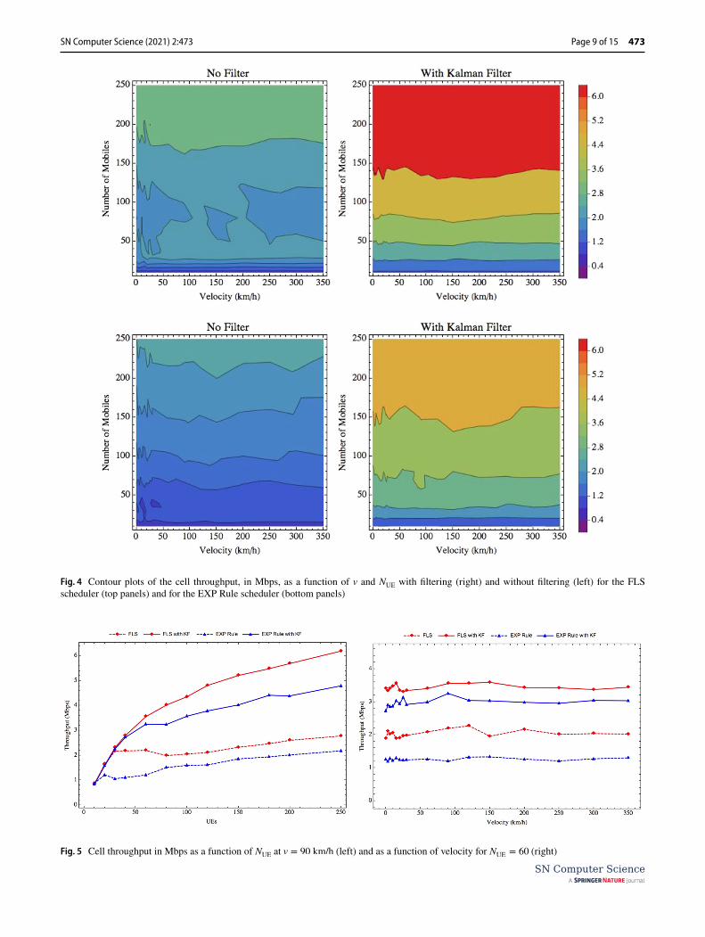
Throughput Performance

Figure 4 shows the effect of KF on cell throughput. When we compare the left panels with the right panels it is evident the benefits of including the filter notably for the FLS. The EXP Rule scheduler, although not achieving data rates as high as the FLS, also shows significant improvement.

The left panel of Fig. 5 shows clearly the improvement in the EXP Rule schedule. For the region until 60 UEs the FLS

Fig. 2 Simulated cell throughput in Mbps (top panels) and packet loss rate (bottom panels) showing the effect of KF in schedulers. Left panels show the original schedulers while right panels display the effect of Kalman filter predictor. In this simulation N

UE= 40

SN Computer Science (2021) 2:473473 Page 8 of 15

SN Computer Science

outperforms the EXP Rule (dashed lines). With the KF both schedulers have similar performance (solid lines). Increasing the number of UEs the FLS outperforms EXP Rule, but the relative improvement of the latest with the filter is signifi-cant. This is shown by the gap between schedulers in right panel of Fig. 5.

PLR Performance

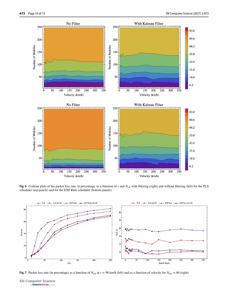
Figure 6 shows simulated measurements of PLR and the effect of the filter. We can readily see the overall improve-ment as the orange–reddish colors representing high PLR in left panels (no predictor) are flushed away in right pan-els (with predictor).

Once more both schedulers benefit from the introduc-tion of KF predictor. In particular, the FLS benefits from filter when the number of UEs is greater than 30 suggest-ing that the scheduler is pre-optimized for a maximum of

Fig. 3 Effect of KF for an application with a given maximum delay. Top panels display the case where the target delay is 0.04 s while bottom panels correspond to a target delay of 0.1 s, for velocities between 0 and 350 km∕h . Left panels show the original schedulers

while right panels display the effect of Kalman filter predictor for a fixed number of 40 UEs. Note that we divided the results of the PF scheduler by ten to compare to the others

Table 2 Simulation parameters

Parameter Value

Bandwidth (MHz) 5.0Resource blocks 25Number of TTI 6000Cell radius (km) 0.5Number of UEs 10, 20, 30, 40, 60, 80, 100,

120, 150, 180, 200 and 250Moving pattern Random directionApplications Video, VoIP and CBRVideo bit rate (kbps) 128Velocity (km/h) 0, 3, 6, 10, 15, 20, 25,

30, 60, 90, 120, 150, 200,250, 300 and 350

Maximum delay (ms) 0.04Schedulers FLS and EXP rule

SN Computer Science (2021) 2:473 Page 9 of 15 473

SN Computer Science

Fig. 4 Contour plots of the cell throughput, in Mbps, as a function of v and NUE

with filtering (right) and without filtering (left) for the FLS scheduler (top panels) and for the EXP Rule scheduler (bottom panels)

Fig. 5 Cell throughput in Mbps as a function of NUE

at v = 90 km/h (left) and as a function of velocity for NUE

= 60 (right)

SN Computer Science (2021) 2:473473 Page 10 of 15

SN Computer Science

Fig. 6 Contour plots of the packet loss rate, in percentage, as a function of v and NUE

with filtering (right) and without filtering (left) for the FLS scheduler (top panels) and for the EXP Rule scheduler (bottom panels)

Fig. 7 Packet loss rate (in percentage) as a function of NUE

at v = 90 km/h (left) and as a function of velocity for NUE

= 60 (right)

SN Computer Science (2021) 2:473 Page 11 of 15 473

SN Computer Science

users/traffic (see left pane of Fig. 7). When the number of users increase the FLS shows effects of filter diminishing the packet loss rate (red solid line).

In its original version, the EXP Rule scheduler drops more packets than FLS during all simulation without pre-dictor (dashed blue line) but when the filter is applied these rates get closer to those from FLS (blue solid line). Right panel of Fig. 7 shows this relative improvement for the EXP rule scheduler and how their performance is simi-lar with the KF.

So, choosing a general propose and relatively simple scheduler such as EXP Rule consistently reduces overall packet losses in the system with the aid of the KF predictor running TTI level without the need of complex algorithms.

The Spectral Efficiency

The quantity spectral efficiency (SE) is a measure of how much data a system can transmit with given bandwidth and its unit is bps∕Hz . In our simulations, we calculated the cell spectral efficiency dividing the total throughput by the simu-lation time and the available bandwidth which is in our case 5 MHz.

In Fig. 8 comparing left with right panels we see again that predictor improve SE for both schedulers. Before the predictor spectral efficiency was around 0.38 bps∕Hz and after prediction, we see values close to 0.6 bps∕Hz . Left pane of Fig. 9 shows that both schedulers have similar SE values as we increased the number of users in simula-tion with and without the KF predictor as seen compar-ing dashed with solid lines. The right pane of same figure

Fig. 8 Contour plots of the spectral efficiency, in bps/Hz, as a function of v and NUE

with filtering (right) and without filtering (left) for the FLS scheduler (top panels) and for the EXP Rule scheduler (bottom panels)

SN Computer Science (2021) 2:473473 Page 12 of 15

SN Computer Science

helps to visualize the gap between the original and modi-fied schedulers.

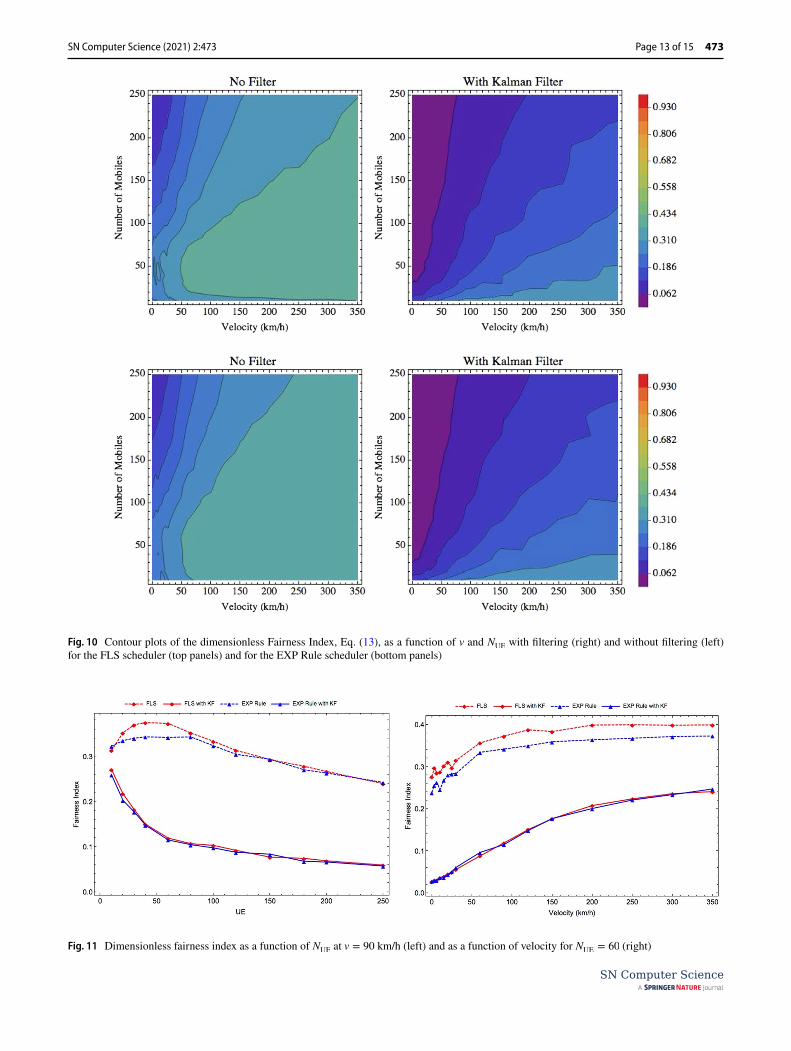
Fairness Index

Jain’s Fairness Index [21] is a quantity representing how equally the resources are allocated among all users in the network and it is given by:

where xi represents the resource consumed by user i.If the network resources have been equally shared, FI = 1 .

However, if the resources are concentrated in a few users, then FI → 1∕N . In Fig. 10 we show the calculated fairness index before and after the introduction of the KF. The first thing to note is that the horizontal patterns seen in previous measurements disappear. The right panel of Fig. 11 shows the sensitivity of Fairness Index (FI) velocity differently from what we observed in previous quantities.

Recalling that we are simulating a single cell with inter-ference, a possible explanation for the dependence on veloci-ties could be that at higher speeds the UEs use cell resources for less time and the schedulers have more spectrum avail-ability. We can also see that the addition of KF degrades by a factor of two the FI meaning that resources are more concentrated among a few users. As the number of users increase, we see that FI quickly decreases (Fig. 11, left pane) showing that all improvements were achieved at the expense of concentrating resources.

(13)FI(x) =1

N

(N∑i=1

xi

)2

×

(N∑i=1

x2i

)−1

,

Conclusions and Outlook

Before reviewing our results, it is important to discuss why the Kalman filter improved the schedulers performance. It is known that the Kalman filter works better when the sys-tem exhibits memory which, in principle, is not the case of scheduling in radio access networks. However, in prac-tice, few allocation types occur for multimedia calls (VoIP, Audio, Video) and in the end, the system behaves as it had some memory.

In this paper, we propose the use of KF to predict the average data rates used by the schedulers algorithm to improve their performance. According to our simulations, the inclusion of the Kalman predictor increases both the throughput and spectral efficiency and reduces the packet loss rate at the cost of fairness in resource allocation.

We also concluded that the best schedulers, when com-petition for resources increase, are the EXP Rule and the FLS (as explained at the end of Sect. 4). It is important to reinforce that the predictive model implemented here in LTE schedulers can be applied to any other system with a centralized resource allocation scheme and therefore can be extended to vehicular, Internet of Things (IoT), 5G networks, and other wideband wireless systems.

A possible reason for the good performance of the EXP Rule is given as follows: examining the M-LWDF and the EXP/PF schedulers we deduce that the �i term is overriding the effect of the predictor. This term is the logarithm of the acceptable packet loss −�i divided by the delay threshold �i for user i. So, the users having less tolerance to delays and requiring low packet loss rates will receive more resources.

Comparing with the LOG rule scheduler, the EXP per-forms better because its metric increases faster than LOG Rule for a given HOL. Also, the denominator of EXP rule normalizes the delay of user i with the delays of all users

Fig. 9 Spectral efficiency in bps/Hz as a function of NUE

at v = 90 km/h (left) and as a function of velocity for NUE

= 60 (right)

SN Computer Science (2021) 2:473 Page 13 of 15 473

SN Computer Science

Fig. 10 Contour plots of the dimensionless Fairness Index, Eq. (13), as a function of v and NUE

with filtering (right) and without filtering (left) for the FLS scheduler (top panels) and for the EXP Rule scheduler (bottom panels)

Fig. 11 Dimensionless fairness index as a function of NUE

at v = 90 km/h (left) and as a function of velocity for NUE

= 60 (right)

SN Computer Science (2021) 2:473473 Page 14 of 15

SN Computer Science

in the network making it a more robust solution compared with LOG Rule [2].

The FLS scheduler also presents good results and this is mostly because it runs on two levels: the low level meaning it acts on TTI and frame level, i.e., working on ten TTIs. This scheduler was designed for real-time video applications and uses as main inputs the queue size and maximum delay for application [2, 19].

Here, we show that the FLS performs well under most cases studied and predictor also improves its performance. Nevertheless, when we use the KF predictor both schedul-ers have similar performances. In other words, applying our predictor to a scheduler that uses a simple metric (EXP Rule) matches the performance of a specialized and comparably complex scheduler (FLS).

The use of our predictor is delay neutral meaning that the schedulers comply with maximum delay required for appli-cation, except for the PF. Fairness in other hand is degraded so some users will show consistently higher throughput that others. A recent work used a fuzzy-logic based packet scheduler which goal is to achieve maximum fairness for a given pool of resources [22]. It would be interesting to check if this approach can equate resources among users without compromising the other performance indicators.

Applying the KF predictor in controlled, test-bed environ-ment can demonstrate the validity of our approach and the real impact on the network processing capacity because the computer will no longer calculate mobility, fading, and other physical aspects of the mobile environment. We also con-sider the introduction of other predictive or machine learning methods if it shows benefits to the system and is sufficiently simple to run on a TTI base.

Finally, we plan to use the Kalman-Takens filter as pre-dictor [23]. With this approach the KF does not require any state model a priori. Using this filter we expect to break the limitations of a fixed state model used for dynamic radio signals therefore expecting to have a more flexible, accurate, and efficient predictor.

Author Contributions MJT: conceptualization, methodology, software, validation, formal analysis, investigation, writing—original draft, visualization. VST: conceptualization, writing—review & editing, supervision.

Funding This work was supported by the Coordenação de Aper-feiçoamento de Pessoal de Nível Superior (CAPES), Finance Code 001, Conselho Nacional de Desenvolvimento Científico e Tecnológico (CNPq) and Fundação de Amparo à Pesquisa do Estado de São Paulo (FAPESP).

Data Availability Not applicable.

Declarations

Conflict of interest/Competing Interests The authors declare no con-flicting/competing interests.

Code availability Code used is available at: https:// github. com/ mteix/ LTESim/ tree/ Kalma nFilt er.

References

1. Ericsson. Ericsson mobility report. 2020. https:// www. erics son. com/ en/ mobil ity- report/ repor ts/ june- 2020.

2. Capozzi F, Piro G, Grieco LA, Boggia G, Camarda P. Downlink packet scheduling in LTE cellular networks: key design issues and a survey. IEEE Commun Surv Tutor. 2013;15(2):678. https:// doi. org/ 10. 1109/ SURV. 2012. 060912. 00100.

3. Abu-Ali N, Taha AEM, Salah M, Hassanein H. Uplink schedul-ing in LTE and LTE-advanced: tutorial, survey and evaluation framework. IEEE Commun Surv Tutor. 2014;16(3):1239. https:// doi. org/ 10. 1109/ SURV. 2013. 1127. 00161http:// ieeex plore. ieee. org/ docum ent/ 66873 13/.

4. Hamza AS, Khalifa SS, Hamza HS, Elsayed K. A survey on inter-cell interference coordination techniques in OFDMA-based cellular networks. IEEE Commun Surv Tutor. 2013;15(4):1642. https:// doi. org/ 10. 1109/ SURV. 2013. 013013. 00028. http:// ieeex plore. ieee. org/ docum ent/ 64760 63/.

5. Luo H, Ci S, Wu D, Wu J, Tang H. Quality-driven cross-layer optimized video delivery over LTE. IEEE Commun Mag. 2010;48(2):102. https:// doi. org/ 10. 1109/ MCOM. 2010. 54026 71. http:// ieeex plore. ieee. org/ docum ent/ 54026 71/.

6. Ameigeiras P, Ramos-Munoz JJ, Navarro-Ortiz J, Mogensen P, Lopez-Soler JM. QoE oriented cross-layer design of a resource allocation algorithm in beyond 3G systems. Comput Commun. 2010;33(5):571. https:// doi. org/ 10. 1016/j. comcom. 2009. 10. 016. https:// linki nghub. elsev ier. com/ retri eve/ pii/ S0140 36640 90028 37.

7. Nasralla MM, Martini MG. 24th International symposium on per-sonal, indoor and mobile radio communications (PIMRC). IEEE (IEEE, 345 E 47TH ST, NEW YORK, NY 10017 USA) 2013; 1571–1575. https:// ieeex plore. ieee. org/ docum ent/ 66663 92.

8. Burchardt H, Sinanovic S, Bharucha Z, Haas H. Distributed and autonomous resource and power allocation for wireless networks. IEEE Trans Commun. 2013;61(7):2758. https:// doi. org/ 10. 1109/ TCOMM. 2013. 053013. 120916. https:// ieeex plore. ieee. org/ docum ent/ 65280 71/.

9. Araniti G, Condoluci M, Iera A, Molinaro A, Cosmas J, Behjati M. A low-complexity resource allocation algorithm for multicast service delivery in OFDMA networks. IEEE Trans Broadcast. 2014;60(2):358. https:// doi. org/ 10. 1109/ TBC. 2014. 23216 78. http:// ieeex plore. ieee. org/ docum ent/ 68236 69/.

10. Trinh HD, Giupponi L, Dini P. 29th IEEE annual international symposium on personal, indoor and mobile radio communica-tions (PIMRC) (IEEE), 2018; 1827–32. https:// ieeex plore. ieee. org/ docum ent/ 85810 00.

11. Ali S, Saad W, Rajatheva N. A directed information learning framework for event-driven M2M traffic prediction. IEEE Com-mun Lett. 2018;22(11):2378. https:// doi. org/ 10. 1109/ LCOMM. 2018. 28680 72.

12. Atawia R, Abou-Zeid H, Hassanein HS, Noureldin A. Joint chance-constrained predictive resource allocation for energy-efficient video streaming. IEEE J Sel Areas Commun. 2016;34(5):1389. https:// doi. org/ 10. 1109/ JSAC. 2016. 25453 58.

SN Computer Science (2021) 2:473 Page 15 of 15 473

SN Computer Science

13. Kalman RE. A new approach to linear filtering and prediction problems. J Basic Eng. 1960;82(1):35.

14. Bishop G, Welch G, et al. An introduction to the Kalman filter. Proc SIGGRAPH Course. 2001;8(27599–3175):59.

15. Acharya J, Gao L, Gaur S. Heterogeneous networks in LTE-advanced. Hoboken: Wiley; 2014.

16. Smith C, Collins D. Wireless networks: design and integration for LTE. EVDO: HSPA, and WiMAX. New York: McGraw-Hill Education LLC; 2014.

17. Swetha Mohankumar N, Devaraju J. Performance evaluation of Round Robin and Proportional Fair scheduling algorithms for con-stant bit rate traffic in LTE. Int J Comput Netw Wirel Commun. 2013;3(1):41.

18. Piro G, Grieco LA, Boggia G, Capozzi F, Camarda P. Simulating LTE cellular systems: an open-source framework. IEEE Trans Veh Technol. 2011;60(2):498. https:// doi. org/ 10. 1109/ TVT. 2010. 20916 60. http:// ieeex plore. ieee. org/ docum ent/ 56341 34/.

19. Piro G, Grieco LA, Boggia G, Fortuna R, Camarda P. Two-level downlink scheduling for real-time multimedia services in LTE networks. IEEE Trans Multimed. 2011;13(5):1052. https:// doi.

org/ 10. 1109/ TMM. 2011. 21523 81. http:// ieeex plore. ieee. org/ docum ent/ 57655 03/.

20. Teixeira MJ, Timoteo VS. 15th International wireless communica-tions and mobile computing conference (IWCMC) (IEEE) 2019; 853–8. https:// doi. org/ 10. 1109/ IWCMC. 2019. 87666 10. https:// ieeex plore. ieee. org/ docum ent/ 87666 10/.

21. Jain RK, Chiu DMW, Hawe WR. Eastern research laboratory. Hudson: Digital Equipment Corporation; 1984.

22. de Souza FR, Duarte-Figueiredo F, Meireles MRG. Telecommu-nication systems. 2020.

23. Hamilton F, Berry T, Sauer T. Ensemble Kalman filtering without a model. Phys Rev X. 2016;6(011021):11021. https:// doi. org/ 10. 1103/ PhysR evX.6. 011021. https:// link. aps. org/ doi/ 10. 1103/ PhysR evX.6. 011021.

Publisher's Note Springer Nature remains neutral with regard to jurisdictional claims in published maps and institutional affiliations.