A Probabilistic Framework for Real-time 3DSegmentation using Spatial, Temporal, and

Semantic CuesDavid Held, Devin Guillory, Brice Rebsamen, Sebastian Thrun, Silvio Savarese

Computer Science Department, Stanford University{davheld, deving, thrun, ssilvio}@cs.stanford.edu

Abstract—In order to track dynamic objects in a robot’senvironment, one must first segment the scene into a collectionof separate objects. Most real-time robotic vision systems todayrely on simple spatial relations to segment the scene into separateobjects. However, such methods fail under a variety of real-world situations such as occlusions or crowds of closely-packedobjects. We propose a probabilistic 3D segmentation method thatcombines spatial, temporal, and semantic information to makebetter-informed decisions about how to segment a scene. Webegin with a coarse initial segmentation. We then compute theprobability that a given segment should be split into multiplesegments or that multiple segments should be merged into asingle segment, using spatial, semantic, and temporal cues. Ourprobabilistic segmentation framework enables us to significantlyreduce both undersegmentations and oversegmentations on theKITTI dataset [3, 4, 5] while still running in real-time. Bycombining spatial, temporal, and semantic information, we areable to create a more robust 3D segmentation system that leadsto better overall perception in crowded dynamic environments.

I. INTRODUCTION

A robot operating in a dynamic environment must identifyobstacles in the world and track them to avoid collisions.Robotic vision systems often begin by segmenting a sceneinto a separate component for each object in the environ-ment [2, 11, 24]. Each component can then be tracked overtime to estimate its velocity and predict where each objectwill move in the future. The robot can use these predictionsto plan its own trajectory and avoid colliding into any staticor dynamic obstacles.

Due to the real-time constraint on these systems, many 3Drobotic perception systems rely on simple spatial relationshipsto find the objects in a scene [2, 11, 14, 24]. For instance, acommon strategy is to use proximity to group points together:if two 3D points are sufficiently close, they are assumed tobe part of the same object, and if the points are far apart anddisconnected, they are assumed to belong to different objects.

However, spatial relations alone are not sufficient for dis-tinguishing between objects in many real-world cases. Forexample, in autonomous driving, it is common for a pedestrianto get undersegmented together with a neighboring object,such as a tree, a nearby car, or a building, as shown inFigure 1 (top). If an autonomous vehicle is not aware of anearby pedestrian, the vehicle will have difficulty anticipatingthe pedestrian’s actions, which could lead to a disastrous

collision. It is also common for a nearby object such as acar to get oversegmented into multiple pieces, with the front,side, and interior of the object being considered as separatesegments (Figure 1, bottom). This oversegmentation can leadto poor tracking estimates, causing the autonomous vehicle toincorrectly predict the future position of nearby objects.

Fig. 1. Top: Using only spatial cues, a person is segmented together with anearby building. By tracking this person over time, we segment it as a separateobject. Bottom: Using only spatial cues, a car is oversegmented into multiplepieces. Using semantic and temporal information, we determine that thesemultiple pieces all belong to a single object. Each color denotes a separateobject instance, estimated by the segmentation algorithm. (Best viewed incolor)

We present the first real-time 3D segmentation algorithmthat combines spatial, temporal, and semantic information ina coherent probabilistic framework. A single frame of anenvironment is often ambiguous, as it can be difficult todetermine if a segment consists of one object or multipleobjects. The temporal cues in our framework allow us toresolve such ambiguities. By watching objects over time, weobtain more information that can help us determine how tosegment the scene.

If we can recognize an object, then we can also incorporatethe object class into our framework to assist our segmentation.At the same time, because we are using a probabilisticframework, the semantic cues are optional, enabling us tosegment unknown objects: if we do not recognize an object,then our semantic probabilities will be uninformative and ourframework will automatically rely on the spatial and temporalinformation for segmentation.

Our method outputs an “instance segmentation”, i.e. apartition of a collection of 3D points into a set of clusters, withone cluster corresponding to each object instance in the scene.These objects can then be individually tracked to estimate theirfuture positions and avoid collisions.

We apply this method to the KITTI dataset, which wascollected from a moving car on crowded city streets forthe purpose of evaluating perception for autonomous driv-ing [3, 4, 5]. We show that our framework significantly reducesboth oversegmentation and undersegmentation errors, withthe total number of errors decreasing by 47%. Our methodruns in only 34 milliseconds per frame (not including theinitial coarse segmentation, which is an input to our methodand requires an additional 19.6 ms) and is thus suitable forreal-time use in robotic applications. By combining spatial,semantic, and temporal information, we are able to createa more robust perception pipeline that should lead to morereliable autonomous driving. More information about ourapproach can be found on our website: http://davheld.github.io/segmentation3D/segmentation3D.html

II. RELATED WORK

Spatial segmentation. Most real-time 3D segmentationmethods only use the spatial distance between points in thecurrent frame for clustering [2, 11, 24], ignoring semanticinformation as well as temporal information from previousframes. However, because these methods only use the spatialdistance between points, they cannot resolve ambiguous caseswhere an occlusion causes an object to become oversegmentedor when multiple nearby objects become segmented together.

Temporal segmentation. Some methods focus on seg-menting objects that are currently moving [1, 17, 27]. Forexample, Petrovskaya and Thrun [17] use “motion evidence”to detect moving vehicles. After filtering out static objects,clustering the remaining moving objects becomes simpler.Another approach is to estimate the motion for each point inthe scene and then to cluster these motions [22, 8]. However,these methods would not be able to segment a stopped car orother objects that are currently stationary but may move in thefuture.

An additional approach is to cluster an image into coherentsuperpixels by enforcing spatial and temporal consistency [9,28, 29]. However, these superpixels do not represent wholeobjects, so a post-processing method must be used to findthe objects in the scene so that each object can be trackedfor autonomous driving or other robotics applications. Further,most of these methods are applied to dense RGB-D imagesfrom indoor scenes [9, 28, 29, 22, 8] and would not directlyapply to large outdoor scenes with sparse 3D sensors.

Semantic segmentation. Other papers have attempted toincorporate semantic information for 3D segmentation. Manyof these methods can only segment objects of particular classesthat can be recognized by a detector [21, 13, 6]. Using ourprobabilistic framework, semantic information is an optionalcue; we are able to use spatial and temporal information

to segment novel objects that we cannot identify, which isimportant for robust autonomous driving in the real world.

Wang et al. [26] use a foreground/background classifierto detect and segment objects. We compare to this methodand demonstrate that we achieve much better performance byalso incorporating temporal information. Further, their methodassumes that foreground objects are well-separated from eachother, which does not hold for crowded urban environments.

Point-wise labeling. Some papers apply a semantic label toeach individual point in the scene [12, 20]. For example, thesemethods will give a label “person” to every point in a crowd ofpedestrians or “car” to every point in a group of cars, withoutlocating the individual objects in this group. The output ofthese methods are less useful for autonomous driving, sincewe need to be able to segment and track each object instancein our environment so we can predict where the object willgo and avoid collisions.

Our approach. We are able to segment both known andunknown objects, as well as objects that are either moving orstationary. Each segment output by our method represents asingle object instance. Our real-time segmentation method isthus suitable for autonomous driving and other mobile robotapplications, in which all objects in our environment must besegmented so we can track each one and avoid collisions.

III. SYSTEM OVERVIEW

Given a stream of input data, we first perform ground-detection, i.e. we determine which points belong to the groundand which points belong to objects. Next, we apply a fastinitial segmentation method to cluster the non-ground pointsinto separate segments (see Section VI-D for details).

We modify these initial segments using our probabilisticframework, splitting segments apart or merging segmentstogether using spatial, temporal, and semantic information.Our framework computes the probability that a set of pointsrepresents a single object or more than object. If we estimatethat a segment consists of more than one object, then we splitthis segment apart; if we estimate that a group of segmentsrepresents a single object, then we merge these segmentstogether. Our goal is to obtain a final set of segments whereeach segment is estimated to represent a single object.

After obtaining the final segmentation for a given frame,each segment is tracked and classified to further improve therobot’s understanding of its environment. Various methodsfor the ground-detection, initial segmentation, tracking, andclassification may be used; the methods used in our pipelineare listed in Section VI-D.

IV. PROBABILISTIC FRAMEWORK

A. Segmentation Model

Our probabilistic framework estimates whether a segmentrepresents a single object or multiple objects, incorporatingthe current observation, the estimated data association, and theestimated segmentation of previous frames. We also optionallyincorporate semantic information if we can recognize the typeof object being segmented, as explained in Section IV-E.

At each time frame i, we observe a set of 3D points.We define a segmentation at frame i as a partitioning of the3D points in frame i into disjoint subsets (“segments”). Werepresent this segmentation as Si = {si,1 · · · si,n}, where eachsegment si,j is a subset of the 3D points observed at frame i.

For the current frame t, St represents our initial segmenta-tion at frame t, whereas for previous frames tj ∈ {1...t− 1},Stj represents the final estimated segmentation at frame tj .For each segment si,j , let zi,j be a set of features (defined inSection IV-D) computed over that segment. Then let Zi be theunion of all of these features, i.e. Zi = {zi,1 · · · zi,n}.

From our initial segmentation St at frame t, let st be aset of segments formed by the union of one or more of ourinitial segments st,j , i.e. st ⊆ St. Further, let zt be a set offeatures computed based on the points in st. We will use theterm “segment” to refer to either a set of points, such as st,j ,or a set of sets of points, such as st.

We want to estimate whether the points in st belong toa single object or more than one object, and based on thisestimate, we will merge the segments in st together into asingle segment, or we can split the segments in st apart intosmaller segments, as explained in Section V. To determinewhether the points in st belong to a single object or morethan one object, we compute a probability p(Nst

t |Z1..t) whereNstt = true if the points in st belong to only one object, and

Nstt = false if the points belong to more than one object. We

make the simplifying assumption that we can compute Nstt

only from the features zt independently from the features ofall other segments at frame t, i.e.

p(Nstt |Z1..t) = p(Nst

t |Z1..t−1, zt). (1)

We abbreviate Nstt as Nt when it is clear which segment it

refers to.

B. Data Association

We accumulate segmentation evidence across time to betterestimate the probability that st consists of only one object.To do so, we incorporate the data association astt , whichrepresents a matching between the points in st in the currentframe and a collection of points in the previous frame t − 1.Suppose that the estimated final segmentation at frame t− 1,given by St−1, is some partition of the points observed atframe t−1 into n segments, St−1 = {st−1,1 · · · st−1,n}. Thenastt is an n-dimensional vector where the ith element is 1 ifa subset of the points in st “match” to a subset of the pointsin st−1,i and 0 otherwise. The data association “matching”indicates that these points belong to the same object or groupof objects viewed at different points in time. An illustrationof the data association is shown in Figure 5.

By determining which points across time correspond tothe same set of objects, the data association creates a setof context-specific independences. Specifically, let astt,i be theith element of astt . If astt,i = 0, then the points in st−1,ido not belong to the same object or group of objects asthe points in st. The 3D points corresponding to differentobjects are assumed to be independent of each other. If we

ft

ft-1,1

at,1=1

...

ft-1,n

at,n=1

...

at,i=1ft-1,i

Fig. 2. The data association at,i creates context-specific independenciesvisualized in this Bayes Net: ft is only dependent on ft−1,i if at,i = 1,indicating that the corresponding 3D points from st and st−1,i may be partof the same object or group of objects.

define ft = {zt, Nt} as the set of variables that correspondto st (and we likewise define ft−1,i to correspond to segmentst−1,i), then ft and ft−1,i are only dependent on each other ifastt,i = 1, indicating that the points in st and st−1,i correspondto the same object or set of objects. Thus we have the context-specific independence

p(ft|astt,i = 0, ft−1,i) = p(ft|astt,i = 0). (2)

This relationship is visualized in Figure 2.For a given value of astt , let st−1 be the set of all segments

from time t− 1 for which the ith element of astt is 1, i.e.

st−1 = {st−1,i : astt,i = 1, i ∈ {1...n}} (3)

where astt,i is the ith element of astt . Further, let zt−1 be thefeatures computed on the set of all points in st−1, let Nt−1indicate whether the points in st−1 constitute a single objector more than one object, and let ft−1 = {zt−1, Nt−1}. Let usfurther define

¬st−1 = {st−1,i : astt,i = 0, i ∈ {1...n}}. (4)

and we similarly define ¬ft−1. Note that St−1 = st−1∪¬st−1.Let us also define Ft−1 = {ft−1,¬ft−1}. Then by applyingequation 2 repeatedly for each i such that astt,i = 0, we havethat

p(ft|astt , Ft−1) = p(ft|astt , ft−1,¬ft−1) (5)= p(ft|astt , ft−1). (6)

In other words, ft is independent of all segments for whichastt,i = 0 and their corresponding features ¬ft−1. We abbrevi-ate astt as at when it is clear which segment it refers to.

The data associations shown in Figure 2 extend backwardthrough time to form a graph, where all nodes at time t−k areconnected to all nodes at time t− k − 1. Performing compu-tations on this graph would be computationally intractable.Instead, we take advantage of the fact that the points inthe previous frames have already been segmented using themethod described in this paper. As a result, each segment from

time t−k (for k ≥ 1) will usually be associated with (at most)a single segment from time t − k − 1 with high probability;if this were not the case, then the segmentation would likelyhave been modified (either splitting or merging segments, asdescribed below) to make this true.

We can take advantage of this property to simplify ourcomputation. For segment st−k (for k ≥ 1), let st−k−1 bethe single most likely associated segment from time t−k−1,with index i. We make the simplifying assumption that thedata association a

st−k

t−k can take on only 2 possible values:either all elements are 0, or element i (corresponding to thesingle most likely associated segment) is equal to 1 and therest are 0. Because we have already segmented frame t−k (andprior frames) using our method, the other data associations areassumed to have sufficiently low probability that they can beignored.

In other words, we assume that only two options are possiblewith high likelihood: either the points in st−k and st−k−1belong to the same object(s), or the points in st−k belong toa new object that appeared at time t− k for the first time. Ineither case, st−k is assumed to be independent of all pointsfrom time t− k− 1 other than those in segment st−k−1. Thisrelationship is visualized in Figure 3.

ft

ft-1,1

at,1=1

...

ft-1,n

at,n=1

...

at,i=1ft-1,i

at-1,1=1ft-2,1

at-2,1=1ft-3,1

...

at-1,i=1ft-2,1

at-2,i=1ft-3,i

...

at-1,n=1ft-2,n

at-2,n=1ft-3,n

...

...

...

...

...

Fig. 3. An extension of Figure 2, we assume that for times t−k (for k ≥ 1)each segment is associated with at most 1 previous segment, given by themost likely data association. The segment is only associated with a previoussegment if at−k,i = 1, as shown by the context-specific independences inthis figure; otherwise the segment is assumed to correspond to a new object.

As shown in Figure 3, the segment st−1,i is thus associatedwith an entire history of segments s1,i...st−2,i, given by themost likely data association at each time step. Similarly, st−1(defined in equation 3) is associated a history of segmentss1...t−2 with features z1..t−2. Further, st−1 is independent ofall prior segments that are not included in s1...t−2. We thushave the independence relationship that

p(ft−1|F1..t−2) = p(ft−1|f1..t−2,¬f1..t−2)

= p(ft−1|f1..t−2) (7)

Based on these independence relationships (shown in Fig-ure 3), we can now extend equation 6 to write

p(ft|astt , F1...t−1) = p(ft|astt , f1...t−1). (8)

The same relationship holds for any subset of the features inft or ft−1, as shown in Figure 3, so we have that

p(zt, Nt|astt , Z1...t−1) = p(zt, Nt|astt , z1...t−1). (9)

and thus by the laws of conditional independences we alsohave that

p(zt|Nt, astt , Z1...t−1) = p(zt|Nt, astt , z1...t−1). (10)

Note that the features zt can be computed directly fromthe observed points st, whereas the boolean variables Ntare unobserved and must be inferred from the observations.Conditioned on the data association at, these variables definea Hidden Markov Model (HMM) shown in Figure 4, where theobserved variables are zt and the hidden variables are Nt. Asnoted above and shown in this figure, the segment st−1 (withcorresponding variables zt−1 and Nt−1) is associated with ahistory of segments s1...st−2 based on the most likely dataassociation, with associated features z1...zt−2 and booleanvariables N1...Nt−2.

NtNt-1Nt-2Nt-3

...

Zt-3 Zt-2 Zt-1 Zt

atat-1at-2

Fig. 4. The Hidden Markov Model (HMM) defined by the observed featureszt and the boolean variable Nt that indicates whether a segment consistsof one object or more than one object. The variables Nt are not observedand must be inferred. The data association at defines the dependency of thesegments across time; see the text for more details.

An example of how the data association can be used forsegmentation is shown in Figure 5. In the top example, thepoints in st have been incorrectly estimated to belong totwo separate objects, even though they are both part of thesame car. However, in the previous time frame, the car wassegmented correctly into a single segment st−1. By associatingthese segments across time, we can obtain a better estimateof whether the points in st should be merged together into asingle segment.

Likewise, the bottom example in Figure 5 shows twopeople that have initially been incorrectly merged into asingle segment st. However, in the previous time frame, thetwo people were each segmented separately. By associatingthese segments across time, we can obtain a better estimateof whether the points in st should be split apart into twoseparate segments. In our framework, we do not assume thatthe previous segmentation was correct; rather, we incorporate aprobabilistic estimate of the previous segmentation to improvethe current segmentation. Below, we will describe how wecompute the probabilities needed to make these decisions.

C. Estimating number of objectsNext we describe how we use our model to estimate Nt,

which indicates whether segment st consists of one object

DataAssocia*onat

stst-1

DataAssocia*onat

st-1,1 stst-1,2

Fig. 5. Top: at time t, a car is initially oversegemented into two pieces.We use our framework to estimate whether these two segments should bemerged together into a single segment st, by matching the segments tocorresponding segments at time t − 1. Bottom: At time t, two people areinitially undersegmented together. We use our framework to estimate whetherthis segment should be split apart, by matching the segment to correspondingsegments at time t−1. Each color represents a separate segment. (Best viewedin color)

or more than one object. We estimate this from the featureszt from the current segment as well as features Z1..t−1 frompast segments. We do not know the true data association forthe current frame, so we sum over different possible dataassociations. Continuing from equation 1, we can write

p(Nt|zt, Z1..t−1) = η1∑at

p(zt|Nt, at, Z1..t−1) p(Nt, at|Z1..t−1)

(11)

where we have expanded the probability using Bayes’ rule,with the normalization constant η1 = 1/p(zt|Z1..t−1). Al-though at can take on 2n possible values, we show a tractableway to compute this in Section VI-A.

The data association at matches the segment st with aprevious segment st−1 that represents the same object orset of objects as the points in st. The segment st−1 has anassociated variable Nt−1 that represents whether the points inst−1 correspond to a single object or to more than one object.We would like to use our estimate of Nt−1 to allow us tobetter estimate Nt. To do so, we can expand the final term ofequation 11 as

p(Nt, at|Z1..t−1) =∑Nt−1

p(Nt, at, Nt−1|Z1..t−1)

=∑Nt−1

p(Nt|at, Nt−1, Z1..t−1)

p(at|Nt−1, Z1..t−1) p(Nt−1|Z1..t−1)(12)

The data association at is a matching between thepoints in st and the points in St−1. Since the probabilityp(at|Nt−1, Z1..t−1) in equation 12 does not condition onany information from segment st, this probability is simply

computed as the prior p(at). We use a constant prior for thedata association, i.e. p(at) = η2, so we have

p(Nt, at|Z1..t−1) = η2∑Nt−1

p(Nt|at, Nt−1, Z1..t−1)

p(Nt−1|Z1..t−1). (13)

Based on the HMM from Figure 4, we also have that

p(Nt|at, Nt−1, Z1..t−1) = p(Nt|at, Nt−1). (14)

Thus we can simplify equation 13 as

p(Nt, at|Z1..t−1) = η2∑Nt−1

p(Nt|at, Nt−1) p(Nt−1|Z1..t−1)

(15)

Using the same assumptions as in equation 1, we can rewritethe final term from equation 15 as

p(Nt−1|Z1..t−1) = p(Nt−1|zt−1, Z1..t−2) (16)

The expression on the right of equation 16 is similar to theexpression on the left side of equation 11 for the previous timestep (replacing t with t− 1), so we compute this recursively,allowing us to accumulate segmentation evidence across time.

The term p(Nt|at, Nt−1) in equation 15 represents theprobability that a segmentation remains consistent across time.This term corresponds to the transition probability in anHMM. Although a segmentation usually remains consistent,sometimes a single object can split to become more thanone object. For example, a person might dismount from abicycle; in this case, a single object (person-riding-bicycle)now becomes two separate objects as the person moves awayfrom the bicycle. Conversely, a person can enter into a car, inwhich case two objects (person and car) are now treated as asingle object.

The overall probability can now be written as:

p(Nt|zt, Z1..t−1) = η∑at

p(zt|Nt, at, z1..t−1)∑Nt−1

p(Nt|at, Nt−1) p(Nt−1|zt−1, Z1..t−2)

(17)

where η = η1 η2. The three terms in equation 17 representour current measurement model, temporal consistency, andour previous estimate, respectively. Note that these termscorrespond to those in the standard update equations for aBayes filter [25].

D. Measurement Model

The term p(zt|Nt, at, z1..t−1) of equation 17 represents theprobability of our current observation’s features zt, knownas a “measurement model”. For segment st, we define zt ={zpt , zst } as a set of features for this segment, where zpt is theposition of the segment’s centroid and zst are a set of featuresthat represent the segment’s shape (defined below).

Assuming that the position and shape are independent, wecan now write this as

p(zt|Nt, at, z1..t−1) = pP (zpt |at, z1..t−1) pS(zst |Nt). (18)

We have eliminated the dependency of the first term on Ntsince the centroid’s position is not dependent on the number ofobjects. We have further simplified our shape probability com-putation by assuming that pS(zst |Nt, at, z1..t−1) = pS(zst |Nt).Although in reality our current shape features zst depend on theprevious shape features zs1..t−1, this conditional independenceassumption will greatly simplify our calculations. These twoterms will be explained in more detail below. The overallprobability can now be written as:

p(Nt|zt, Z1..t−1) =η∑at

pP (zpt |at, z1..t−1) pS(zst |Nt)∑Nt−1

p(Nt|at, Nt−1) p(Nt−1|zt−1, Z1..t−2).

(19)

1) Position Probability: In equation 19, we sum over thedifferent possible data associations at. Each data associationrepresents a matching between the set of points st and aprevious set of points, st−1 (where st−1 might be a unionof one or more of our previous segments). However, someof the data associations are more likely than others. Theprobability pP (zpt |at, z1..t−1) in equation 19 will allow us toweight more highly the terms in the summation correspondingto more likely data associations and down-weight the termscorresponding to less likely data assocations.

The position probability, pP (zpt |at, z1..t−1), is computedfrom the position of the (noisy) centroid observation zptcompared to its predicted position, based on the estimatedobject velocity. We represent the object state xt as its positionand velocity, and we integrate over the different states xt:

pP (zpt |at, z1..t−1) =

∫xt

p(zpt |xt) p(xt|at, z1..t−1) dxt. (20)

This probability is computed using a Kalman Filter [25]. Weassume that we have modeled the previous distribution overobject states p(xt−1|z1..t−1) as a Gaussian with mean µ andcovariance Σ.

To compute this integral, we first perform the Kalman Filterprediction step to get a prediction of the object’s currentposition and velocity (see [25] for details). The resultingprediction is given by a Gaussian with mean µ = [µv, µx] andcovariance Σ, with the predicted mean velocity and positiongiven by µv and µx respectively. If we model the measurementprobability p(zpt |xt) by a Gaussian with measurement noise Q,then equation 20 is the convolution of two Gaussians, whichresults in another Gaussian. The probability is thus given by

pP (zpt |at, z1..t−1) = N (zpt ; µ, Σ +Q). (21)

To compute this probability, we first shift the point cloudfrom segment st−1 to its predicted position µx to get thepredicted point cloud st. Next, we find the point pi ∈ st that

is nearest to the centroid zpt . We then compute the probabilityas

pP (zpt |at, z1..t−1) = C1 exp(− 1

2(zpt − pi)TΣ−1(zpt − pi)

)(22)

where C1 = η3 |Σ|−1/2 and Σ = Σ + Q (and η3 is anormalization constant). We find that using the entire predictedpoint cloud st is more robust than simply using its centroid.

2) Shape Probability: The second term of equation 19,pS(zst |Nt), is the probability of observing a measurementwith shape features zst (defined below) conditioned on thenumber of objects in the points st. This probability is themain term in equation 19 that directly relates to the number ofobjects; the other terms are used to accumulate segmentationevidence across time. Without any semantic information, thisprobability is based only on the distance between points, as isnormally used in spatial clustering [2, 11, 24]. However, in ourframework, this probability is accumulated across time to givea more accurate segmentation, as described in Section IV-C.

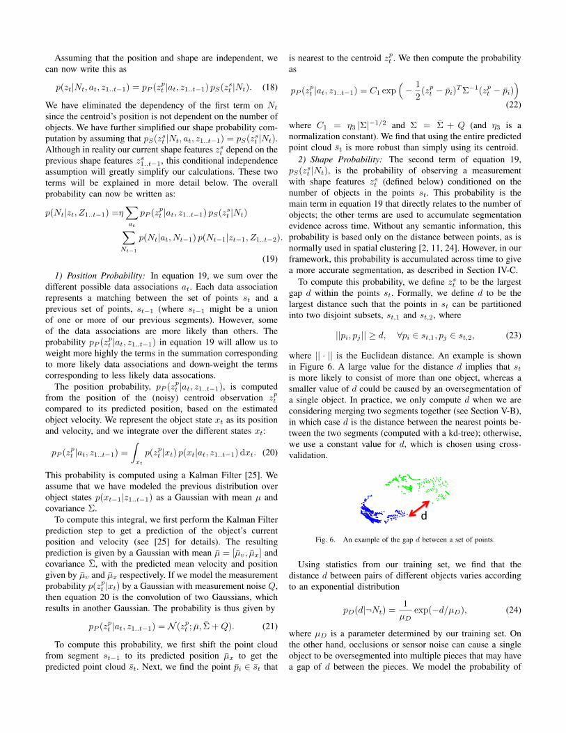
To compute this probability, we define zst to be the largestgap d within the points st. Formally, we define d to be thelargest distance such that the points in st can be partitionedinto two disjoint subsets, st,1 and st,2, where

||pi, pj || ≥ d, ∀pi ∈ st,1, pj ∈ st,2, (23)

where || · || is the Euclidean distance. An example is shownin Figure 6. A large value for the distance d implies that stis more likely to consist of more than one object, whereas asmaller value of d could be caused by an oversegmentation ofa single object. In practice, we only compute d when we areconsidering merging two segments together (see Section V-B),in which case d is the distance between the nearest points be-tween the two segments (computed with a kd-tree); otherwise,we use a constant value for d, which is chosen using cross-validation.

d

Fig. 6. An example of the gap d between a set of points.

Using statistics from our training set, we find that thedistance d between pairs of different objects varies accordingto an exponential distribution

pD(d|¬Nt) =1

µDexp(−d/µD), (24)

where µD is a parameter determined by our training set. Onthe other hand, occlusions or sensor noise can cause a singleobject to be oversegmented into multiple pieces that may havea gap of d between the pieces. We model the probability of

observing an oversegmentation of a single object with a gapof d between two pieces by an exponential distribution

pD(d|Nt) =1

µSexp(−d/µS), (25)

where µS is determined using cross-validation on our trainingset. Typically we have that µD > µS based on the intuitiondescribed above: a larger gap between points is indicativethat the points may belong to multiple objects. The shapeprobability is then set to be equal to this distribution:

pS(zst |Nt) = pD(d|Nt). (26)

E. Semantics

In the previous sections we have used spatial and temporalinformation (accumulating segmentation evidence across time)to estimate the segmentation. In this section we show how toincorporate semantic information: if we can recognize the typeof object for a given segment, this should give us additional in-formation about how to segment the scene. On the other hand,if we cannot recognize the object, then the probabilistic modelnaturally reverts to the model of Sections IV-A through IV-Dthat incorporates only spatial and temporal information.

We assume that we have a segment classifier p(c|zc1..t) thatcomputes the probability that the set of segments s1..t is someclass c, based on a set of features zc1..t. To use the classifier, wemust sum over class labels. Equation 11 can now be rewrittenas

p(Nt|zt, Z1..t−1) =η1∑at

∑c

p(zt|Nt, at, c, Z1..t−1)

p(Nt, at, c|Z1..t−1). (27)

The second term of equation 27 can be expanded as

p(Nt, at, c|Z1..t−1) = p(Nt, at|Z1..t−1) p(c|Nt, at, Z1..t−1).(28)

For the second term of equation 28, if the data associationis given then the class label c is only dependent on the cor-responding matching segments s1..t−1 (based on equation 8),so we compute this term as p(c|at, zc1..t−1) using the segmentclassifier.

We now compute a more accurate measurement probability,since we are also conditioning on the class label c. Forexample, we now compute equation 25 as

pD(d|Nt, c) =1

µS,cexp(−d/µS,c), (29)

where the parameter µS,c can vary based on the class label.For example, for a car, an oversegmentation might reasonablycause a 15 cm gap between points, whereas for a single person,only a 3 cm gap might be considered reasonable. We chooseµS,c for each class using cross-validation on the training set.

We also incorporate more information about the objectshape into the computation of pS(zst |Nt, c), since we areconditioning on the object class. Although a complex shapemodel can be used, for sake of efficiency we use the volumetricsize of the segment st. We first compute the length and width

(l1, l2) of a bounding box fit to the segment st. We nowdefine zst to be the set {d, l1, l2}, where d was defined inSection IV-D2. For each class, we model the size of an averagesegment for that class by a Gaussian with parameters µi,c andσi,c along each dimension i. However, a partially occludedsegment may appear smaller than this; thus, we compute theprobability along each dimension as

pV (li|Nt, c) = η4

{exp

(−(li−µi,c)

2

2σ2i,c

), if li ≥ µi,c

1, otherwise.(30)

where η4 is a normalization constant. If Nt = false (i.e. thepoints in st consist of more than one object), we expect thesegment to be bigger than average with a large variance. Wethus compute this probability as

pV (li|¬Nt, c) = N (li;µ′i,c, σ

′i,c) (31)

with µ′i,c = k1µi,c and σ′i,c = k2σi,c for constants k1, k2 > 1chosen using cross-validation on our training set. We can nowreplace the shape probability from equation 26 with

pS(zst |Nt, c) =pD(d|Nt, c)∏i

pV (li|Nt, c). (32)

Note that one of the classes may be “unknown.” When wecondition on the “unknown” class, then the size probabilitypV (li|Nt, c) will be uninformative; however, the probabilisticmodels from Sections IV-A through IV-D are still used. Thus,our segmentation model benefits when we recognize the objectclass, but we can still segment the scene even for unknownobjects.

V. SEGMENTATION ALGORITHM

We now describe how we use the probabilistic modeldescribed above, combining spatial, temporal, and (optionally)semantic information to improve our scene segmentation.

A. Splitting

After obtaining an initial coarse segmentation, we iterateover all of our initial segments st and compute the probabilityp(Nt|zt, Z1..t−1) using equation 19 to determine whether thesegment should be further split. Although the initial coarsesegmentation might only use spatial information, the com-putation of p(Nt|zt, Z1..t−1) also incorporates semantic andtemporal information, allowing us to make a more informeddecision about how to segment the points in st. We definedNt = false if the points in st belong to more than oneobject. Thus if p(¬Nt|zt, Z1..t−1) > 0.5, we conclude thatthe segment st represents more than one object and shouldbe split into smaller segments. The details of this splittingoperation are explained in Section VI-C.

B. Merging

After all of our segments have been split using spatial,semantic, and temporal information, some objects may havebecome oversegmented. We now use our probabilistic modelto determine when to merge some of these segments backtogether. To do this, we iterate over pairs of segments st,i

and st,j , and we propose a merge of these segments to createa single merged segment st,ij = st,i ∪ st,j with featureszt,ij . We then compute the probability p(Nt|zt,ij , Z1..t−1) forthis proposed merged segment, again using equation 19. Ifp(Nt|zt,ij , Z1..t−1) > 0.5, then we conclude that these twosegments are actually part of one object and we merge themtogether; otherwise, we keep these two segments separate. Wecontinue to merge segments until no more segments can bemerged, meaning that our segmentation has converged.

VI. IMPLEMENTATION DETAILS

A. Approximations

In order to make our method run in real-time, we haveto perform a number of approximations. For example, inequation 11, we sum over all data associations for segment st.However, segment st can match to any number of segmentsfrom the previous frame; if there are n segments in theprevious frame, then there are 2n possible data associations.

However, it is not necessary to compute all of these as-sociations, since we only want to know whether segment stconsists of one object or more than object. Therefore, wesimplify the problem by only considering matches to eithersingle segments, to pairs of segments, or to no segments fromthe previous frame. Formally, we only consider values of atwhere 0, 1, or 2 elements are equal to 1 and the rest are equalto 0. Thus we only need to consider n2 +n+ 1 potential dataassociations, making this summation much faster to compute.Further, if a segment from the previous frame is sufficientlyfar away from the current segment, then it will likely notcontribute very much to this probability, so we do not need toconsider this segment for data association.

Additionally, when we match to a single segment in theprevious frame, we use the prior probability in the recursivecomputation, i.e. p1(Nt−1|zt−1, Z1..t−2) ≈ p1(Nt−1), whichspeeds up our method at little cost in accuracy. We still com-pute the probability p(Nt−1|zt−1, Z1..t−2) recursively whenwe consider a data association to multiple prior segments.

We precompute the class probability p(c|at, zc1..t−1) foreach individual segment st−1. For efficiency reasons, wetherefore do not use semantics when conditioning on a valueof at such that st matches to more than one previous segment.

B. Lazy computation

Normally, when using a Bayes filter, we take advantage ofthe Markov property: when computing frame t, we only needinformation from frame t − 1, so we do not need to keepany information from prior frames. Normally, one would pre-compute all information at time t− 1 that one might need fortime t. However, in our segmentation framework, we only needa subset of the information from the previous frame, but wecannot determine which subset in advance. Thus, we insteadperform a lazy computation: we keep the last T frames of data,and we make use of the prior information only as needed forour recursive computation p(Nt−1|zt−1, Z1..t−2). This allowsour method to be much more efficient, because we do not

perform computations from prior frames that are not neededby our framework.

C. Splitting Operation

As described above, we use our probabilistic frameworkto decide which segments st represent more than one objectand therefore must be split into smaller segments. Once thedecision to split segment st is made, the segment can be splitusing a variety of methods. We split the segment using spatialand temporal information as described below.

1) Temporal Splitting: At a high level, our temporal split-ting method matches the segment st in the current frame tosegments from the previous frame. If more than one segmentfrom the previous frame matches to segment st with highprobability, then we split st based on the shape of thoseprevious segments. For example, if a crowd of pedestriansin the current frame matches to separate pedestrian segmentsin the previous frame, then we try to associate each 3D pointin the crowd to a 3D point in an individual pedestrian in theprevious frame. We then use the associations to split the crowdinto multiple segments, where each segment consists of all3D points that were matched to the same previously observedpedestrian.

Specifically, we first find the segments st−1,1 · · · st−1,nfrom the previous frame that have a strong match to thesegment st in the current frame according to equation 22. Next,we compute whether these segments from the previous frameare likely to represent different objects; they may have merelybeen the result of a previous oversegmentation. To do this, wetake all pairs of these matching segments st−1,i and st−1,j andwe merge each pair into a single segment st−1,ij . We thencompute p(Nt−1|zt−1,ij , S1..t−2) for this merged segmentusing equation 19. If p(¬Nt−1|zt−1,ij , S1..t−2) > 0.5, then weassume that st−1,i and st−1,j belong to two different objectsand can be used for temporal splitting. We then find the setof all such segments st−1,1 · · · st−1,m with a strong match tost that are all estimated to represent different objects.

To perform the split, for each point in the current framepi ∈ st, we compute the probability pP (pi|at, z1..t−1,j) usingequation 22 that this point matches to each segment st−1,jfrom the previous frame. We assign point pi to the segmentwith the highest probability, and then the point assignmentsdefine a set of m new segments that get created. Usingthis approach, we split segment st into m new segments bymatching the points in st to segments from the previous frame.

2) Spatial Splitting: The temporal splitting process de-scribed above may not lead to the segment st being splitinto multiple segments, for various reasons. For example, thesegment st may not match to multiple previous segment withhigh probability.

In such a case, we will split segment st using spatialinformation, using a smaller threshold than was used in ourinitial segmentation. Note that we would not want to applysuch a small threshold to all segments; however, we havedetermined using semantic and temporal information thatsegment st is too large, so a smaller threshold may be used. In

our implementation, we split segment st using the Euclideanclustering method in PCL [18, 19], with a clustering thresholdbased on the sensor resolution r, ensuring that all points ineach segment are at least a distance of k3 r from all pointsin a neighboring segment, for some constant k3 chosen usingour training set.

D. Pre- and Post-processing

As a pre-processing step, we remove the points that belongto the ground using the method of Montemerlo et al. [15]. Theinitial coarse segmentation for our method is obtained usingthe Flood-fill method of Teichman et al. [24], extended touse a 3D obstacle grid. After segmentation, we perform dataassociation using the position probability of Section IV-D1.We next estimate a velocity for each object using the trackerof Held et al. [7]. Finally, we classify these segments using theboosting framework of Teichman and Thrun [23], and we usethe same classes as in that reference: pedestrians, bicyclists,cars, and background (which we refer to as unknown). Thevelocity and classification estimates are used to provide tem-poral and semantic cues to improve the segmentation, as wehave described. We find the components listed here to be bothfast and accurate; however, any method for ground-detection,tracking, the initial coarse segmentation, and 3D classificationmay be used.

VII. EVALUATION

Below we discuss our quantitative evaluation. A videodemonstrating our segmentation performance can be found onthe project website.

Dataset: We evaluate our segmentation method on theKITTI tracking dataset [3, 4, 5]. The KITTI dataset wascollected from a moving car on city streets in Karlsruhe,Germany for the purpose of evaluating perception for au-tonomous driving. The 3D point clouds are recorded with aVelodyne HDL-64E 64-beam LIDAR sensor, which is oftenused for autonomous driving [15, 16, 26]. This dataset ispublicly available and consists of over 42,000 3D boundingbox labels on almost 7,000 frames across 21 sequences.Although the bounding boxes do not create point-wise accuratesegmentation labels, the segments produced by these boundingboxes are sufficiently accurate to evaluate our method.

We use 2 of these sequences to train our method and selectparameters, and the remaining 19 sequences are used fortesting and evaluation. The specific parameter values chosenusing our training set are listed in the project website.

Although the KITTI tracking dataset has been made publiclyavailable, the dataset has typically been used to evaluate onlytracking and object detection rather than evaluating segmenta-tion directly. However, segmentation is an important step of a3D perception pipeline, and errors in segmentation can causesubsequent problems for other components of the system.Because the KITTI dataset is publicly available, we encourageother researchers to evaluate their 3D segmentation methodson this dataset using the procedure that we describe here.

Evaluation Metric: The output of our method is a par-titioning of the points in each frame into disjoint subsets(“segments”), where each segment is intended to representa single object instance. The KITTI dataset has labeled asubset of objects with a ground-truth bounding box, indicatingthe correct segmentation. We wish to evaluate how well oursegmentation matches the ground-truth for the labeled objects.

To evaluate our segmentation, we first find the segmentfrom our segmentation that best matches to each ground-truthbounding box. For each ground-truth bounding box gt, letCgt be the set of non-ground points within this box. For eachsegment s from our segmentation, let Cs be the set of pointsthat belong to this segment. We then find the segment that bestmatches to this ground-truth bounding box by computing

s = arg maxs′

|Cs′ ∩ Cgt| (33)

The best-matching segment is then assigned to this ground-truth bounding box for the evaluation metrics described below.

We describe on the project website how the intersection-over-union metric on 3D points [26] is non-ideal for au-tonomous driving because this score penalizes undersegmen-tation errors more than oversegmentation errors. Instead, wepropose to count the number of oversegmentation and under-segmentation errors directly. Roughly speaking, an underseg-mentation error occurs when an object is segmented togetherwith a nearby object, and an oversegmentation error occurswhen a single object is segmented into multiple pieces. Moreformally, we count the fraction of undersegmentation errors as

U =1

N

∑gt

1( |Cs ∩ Cgt|

|Cs|< τu

)(34)

where 1 is an indicator function that is equal to 1 if the inputis true and 0 otherwise and τu is a constant threshold. Wecount the fraction of oversegmentation errors as

O =1

N

∑gt

1( |Cs ∩ Cgt||Cgt|

< τo

), (35)

where τo is a constant threshold. In our experiments, wechoose τu = 0.5 to allow for minor undersegmentation errorsas well as errors in the ground-truth labeling. We use τo = 1,since even a minor oversegmentation error causes a new (false)object to be created. We do not evaluate oversegmentations orundersegmentations when two ground-truth bounding boxesoverlap. In such cases, it is difficult to tell whether thesegmentation result is correct without more accurate ground-truth segmentation annotations (i.e. point-wise labeling insteadof bounding boxes). Examples of undersegmentation and over-segmentation errors are shown in Figure 7.

We then compute an overall error rate based on the totalnumber of undersegmentation and oversegmentation errors, as

E = U + λcO (36)

where λc is a class-specific weighting parameter that penalizesoversegmentation errors relative to undersegmentation errors.For our experiments we simply choose λc = 1 for all classes,

Undersegmenta+on Correct

Oversegmenta+on Correct

Fig. 7. Examples of an undersegmentation error (top) and an oversegmenta-tion error (bottom). Each color denotes a single segment, and the ground-truthannotations are shown with a purple box, where each box represents a singleobject instance. (Best viewed in color)

but λc can also be chosen for each application based on theeffect of oversegmentation and undersegmetation errors foreach class on the final performance.

VIII. RESULTS

Baselines: We compare our segmentation method to anumber of baseline methods. First, we compare to the Flood-fill method of Teichman et al. [24], which is also used as apre-processing step for our method. We also compare to theEuclidean Clustering (EC) method of Rusu [18], which wasapplied to segmentation of urban scenes in Ioannou et al. [10].We evaluate the method of Rusu [18] using cluster tolerancesof 0.1 m, 0.2 m, or 1 m (EC 0.1, EC 0.2, EC 1).

Finally, we compare to the method of Wang et al. [26],which also incorporates semantic information into the segmen-tation. Because the code of Wang et al. [26] was not available,we re-implemented their method. We classify segments usingthe method of Teichman and Thrun [23]. The initial segmenta-tion for this method is obtained using Flood-fill [24], and thepost-processing step is obtained using Euclidean Clusteringwith a dynamic cluster tolerance chosen based on the sensorresolution. This setup was the best-scoring implementation oftheir method that we were able to achieve. We experimentwith three different parameter settings for this method (Wang1,Wang2, Wang3).

Baseline Comparison: Our method operates on the fullpoint-cloud in real-time, and we improve the segmentationat all distances. However, our analysis focuses on segmentswithin 15 m because these are the objects that our autonomousvehicle will most immediately encounter.

The segmentation evaluation is shown in Figure 8, forsegments within 15 m. Combining oversegmentation and un-dersegentation errors, our method has the lowest error rate of10.2%, compared to the Flood-fill baseline [23] with 19.4%.Our method thus reduces the total number of oversegmentationand undersegmentation errors by 47%, demonstrating the ben-efit of combining spatial, temporal, and semantic informationfor 3D segmentation. Our method runs in real-time, taking anaverage of 33.7 ms per frame, or 29.7 Hz, not including theinitial coarse segmentation of [24] which requires an additional19.6 ms.

0 10 20 300

5

10

15

20

25

30

35

% Undersegmentation Errors

% O

vers

egm

enta

tion

Erro

rs

Baseline − Flood−fillBaseline − EC 0.1Baseline − EC 0.2Baseline − EC 1Baseline − Wang1Baseline − Wang2Baseline − Wang3Ours

Fig. 8. Oversegmentation vs Undersegmentation errors for a variety ofsegmentation methods. Best-performing methods appear in the lower-leftcorner of the graph.

The Euclidean Clustering baselines achieved error rates of23%, 26%, or 40% (for different parameter settings). Themethod of Wang et al. [26] achieved error rates of 20.9%,21.3% or 22.3% (for different parameter settings). Althoughthis method incorporates semantic information, they makeassumptions that do not hold in crowded environments. Theirmethod assumes that, after removing the ground points andbackground objects, the remaining foreground objects can besegmented using a spatial clustering approach. Their underly-ing assumption is that foreground objects tend to remain sep-arated from each other in 3D space. Although this assumptionmay hold true for cars, it does not hold true for pedestrians,which often stand in crowds. Furthermore, pedestrians andbicyclists may move close to parked cars, or they may movepast cars at a cross-walk, causing the assumptions of thismethod to fail to hold.

Ablative analysis: To understand the cause for the improve-ment in performance, we separately analyze the benefit ofusing only temporal information and only semantic informa-tion, shown in Table I. As can be seen, adding either temporalor semantic information alone results in small improvementsin performance. However, the largest gains are achieved bycombining spatial, semantic, and temporal information, thusshowing that all three components are important for theaccuracy of our system.

Method % Errors (< 15 m) % Errors (all)Spatial only [24] 19.4 11.6Spatial + Temporal 16.4 10.8Spatial + Semantic 15.4 10.8Spatial + Semantic + Temporal 10.2 8.2

TABLE ISEGMENTATION ACCURACIES FOR VARIOUS VERSIONS OF OUR METHOD.

Performance Analysis: We evaluate the effect of classi-fication on segmentation by separately evaluating our seg-mentation performance on objects that we classify correctlycompared to objects that we classify incorrectly. For objects

that we classify correctly, we reduce the segmentation errorsby 48.4%, compared to 5.8% for objects that we classifyincorrectly (for objects at all distances). Thus, improving theclassification accuracy can lead to significant gains in oursegmentation performance, when using our method whichcombines spatial, temporal, and semantic information.

Effect on Tracking: Finally, we show the effect of seg-mentation accuracy on object tracking. In the KITTI trackingdataset, the ground-truth bounding boxes are also annotatedwith object IDs, so we are able to compute the number ofID switches of our system. Using our segmentation method,we get 25% fewer ID switches compared to the baseline [24]Thus, accurate segmentation is also important for accuratetracking. Because segmentation occurs at the beginning ofthe perception pipeline, errors in segmentation can propagatethroughout the rest of the system, and improving segmentationwill improve other aspects of the system such as tracking, aswe have shown.

IX. CONCLUSION

To perform accurate 3D segmentation, it is not sufficient toonly use the spatial distance between points, as there will bemany ambiguous cases caused by occlusions or neighboringobjects. Our method is able to incorporate spatial, semantic,and temporal cues in a coherent probabilistic framework for3D segmentation. We are able to significantly reduce the num-ber of segmentation errors while running in real-time. Roboticsystems should thus combine spatial, temporal, and semanticinformation to achieve accurate real-time segmentation andmore reliable perception in dynamic environments.

REFERENCES

[1] Asma Azim and Olivier Aycard. Detection, classificationand tracking of moving objects in a 3d environment. InIntelligent Vehicles Symposium (IV), 2012 IEEE, pages802–807. IEEE, 2012.

[2] Bertrand Douillard, James Underwood, Noah Kuntz,Vsevolod Vlaskine, Alastair Quadros, Peter Morton, andAlon Frenkel. On the segmentation of 3d lidar pointclouds. In Robotics and Automation (ICRA), 2011 IEEEInternational Conference on, pages 2798–2805. IEEE,2011.

[3] Jannik Fritsch, Tobias Kuehnl, and Andreas Geiger. Anew performance measure and evaluation benchmark forroad detection algorithms. In International Conferenceon Intelligent Transportation Systems (ITSC), 2013.

[4] Andreas Geiger, Philip Lenz, and Raquel Urtasun. Arewe ready for autonomous driving? the kitti vision bench-mark suite. In Conference on Computer Vision andPattern Recognition (CVPR), 2012.

[5] Andreas Geiger, Philip Lenz, Christoph Stiller, andRaquel Urtasun. Vision meets robotics: The kitti dataset.International Journal of Robotics Research (IJRR), 2013.

[6] Saurabh Gupta, Ross Girshick, Pablo Arbelaez, and Jiten-dra Malik. Learning rich features from rgb-d images for

object detection and segmentation. In Computer Vision–ECCV 2014, pages 345–360. Springer, 2014.

[7] David Held, Jesse Levinson, Sebastian Thrun, and SilvioSavarese. Combining 3d shape, color, and motion forrobust anytime tracking. In Proceedings of Robotics:Science and Systems, Berkeley, USA, July 2014.

[8] Evan Herbst, Xiaofeng Ren, and Dieter Fox. Rgb-d flow: Dense 3-d motion estimation using color anddepth. In Robotics and Automation (ICRA), 2013 IEEEInternational Conference on, pages 2276–2282. IEEE,2013.

[9] Steven Hickson, Stan Birchfield, Irfan Essa, and HelenChristensen. Efficient hierarchical graph-based segmen-tation of rgbd videos. In Computer Vision and PatternRecognition (CVPR), 2014 IEEE Conference on, pages344–351. IEEE, 2014.

[10] Yani Ioannou, Babak Taati, Robin Harrap, and MichaelGreenspan. Difference of normals as a multi-scaleoperator in unorganized point clouds. In 3D Imaging,Modeling, Processing, Visualization and Transmission(3DIMPVT), 2012 Second International Conference on,pages 501–508. IEEE, 2012.

[11] Klaas Klasing, Dirk Wollherr, and Martin Buss. Aclustering method for efficient segmentation of 3d laserdata. In ICRA, pages 4043–4048, 2008.

[12] Abhijit Kundu, Yin Li, Frank Dellaert, Fuxin Li, andJames M Rehg. Joint semantic segmentation and 3dreconstruction from monocular video. In ComputerVision–ECCV 2014, pages 703–718. Springer, 2014.

[13] Kevin Lai, Liefeng Bo, Xiaofeng Ren, and Dieter Fox.Detection-based object labeling in 3d scenes. In Roboticsand Automation (ICRA), 2012 IEEE International Con-ference on, pages 1330–1337. IEEE, 2012.

[14] John Leonard, Jonathan How, Seth Teller, Mitch Berger,Stefan Campbell, Gaston Fiore, Luke Fletcher, EmilioFrazzoli, Albert Huang, Sertac Karaman, et al. Aperception-driven autonomous urban vehicle. Journal ofField Robotics, 25(10):727–774, 2008.

[15] Michael Montemerlo, Jan Becker, Suhrid Bhat, HendrikDahlkamp, Dmitri Dolgov, Scott Ettinger, Dirk Haehnel,Tim Hilden, Gabe Hoffmann, Burkhard Huhnke, et al.Junior: The stanford entry in the urban challenge. Journalof field Robotics, 25(9):569–597, 2008.

[16] Frank Moosmann and Christoph Stiller. Joint self-localization and tracking of generic objects in 3d rangedata. In Robotics and Automation (ICRA), 2013 IEEEInternational Conference on, pages 1146–1152. IEEE,2013.

[17] Anna Petrovskaya and Sebastian Thrun. Model basedvehicle detection and tracking for autonomous urbandriving. Autonomous Robots, 26(2-3):123–139, 2009.

[18] Radu Bogdan Rusu. Semantic 3D Object Maps forEveryday Manipulation in Human Living Environments.PhD thesis, Computer Science department, TechnischeUniversitaet Muenchen, Germany, October 2009.

[19] Radu Bogdan Rusu and Steve Cousins. 3D is here: Point

Cloud Library (PCL). In IEEE International Conferenceon Robotics and Automation (ICRA), Shanghai, China,May 9-13 2011.

[20] Sabyasachi Sengupta, Eric Greveson, Ali Shahrokni, andPhilip HS Torr. Urban 3d semantic modelling usingstereo vision. In Robotics and Automation (ICRA),2013 IEEE International Conference on, pages 580–585.IEEE, 2013.

[21] Luciano Spinello, Kai Oliver Arras, Rudolph Triebel, andRoland Siegwart. A layered approach to people detectionin 3d range data. In AAAI, 2010.

[22] Jorg Stuckler and Sven Behnke. Efficient dense rigid-body motion segmentation and estimation in rgb-d video.International Journal of Computer Vision, pages 1–13,2015.

[23] Alex Teichman and Sebastian Thrun. Group induction. InIntelligent Robots and Systems (IROS), 2013 IEEE/RSJInternational Conference on, pages 2757–2763. IEEE,2013.

[24] Alex Teichman, Jesse Levinson, and Sebastian Thrun.Towards 3d object recognition via classification of arbi-trary object tracks. In Robotics and Automation (ICRA),2011 IEEE International Conference on, pages 4034–4041. IEEE, 2011.

[25] Sebastian Thrun, Wolfram Burgard, and Dieter Fox.Probabilistic robotics. MIT press, 2005.

[26] Dominic Zeng Wang, Ingmar Posner, and Paul Newman.What could move? finding cars, pedestrians and bicyclistsin 3d laser data. In Robotics and Automation (ICRA),2012 IEEE International Conference on, pages 4038–4044. IEEE, 2012.

[27] Nicolai Wojke and M Haselich. Moving vehicle detectionand tracking in unstructured environments. In Roboticsand Automation (ICRA), 2012 IEEE International Con-ference on, pages 3082–3087. IEEE, 2012.

[28] Chenliang Xu, Caiming Xiong, and Jason J Corso.Streaming hierarchical video segmentation. In ComputerVision–ECCV 2012, pages 626–639. Springer, 2012.

[29] Chenliang Xu, Spencer Whitt, and Jason J Corso. Flatten-ing supervoxel hierarchies by the uniform entropy slice.In Computer Vision (ICCV), 2013 IEEE InternationalConference on, pages 2240–2247. IEEE, 2013.