a process for separation by semi-continuous counter

A Process for Separation by Semi-Continuous

Counter-Current Crystallization

By

Nathan M. Aumock

B.S. Chemical Engineering - University of Wisconsin, 2004

M.S. Chemical Engineering Practice - Massachusetts Institute of Technology, 2006

Submitted to the Department of Chemical Engineering in partial fulfillment of the requirements for the degree of

Doctor of Philosophy at the

Massachusetts Institute of Technology

February 2011

© 2011 Massachusetts Institute of Technology. All rights reserved.

Signature of Author .………………………………………………………………………………………………………………………………… Department of Chemical Engineering

December 23, 2010

Certified by ……………………………………………………………………………………………………………………………………………… T. Alan Hatton

Ralph Landau Professor of Chemical Engineering Practice Thesis Supervisor

Certified by ……………………………………………………………………………………………………………………………………………… Kenneth A. Smith

Gilliland Professor of Chemical Engineering Thesis Supervisor

Accepted by ……………………………………………………………………………………………………………………………………………. William M. Deen

Professor of Chemical Engineering Chairman, Committee for Graduate Students

3

A Process for Separation by Semi-Continuous Counter-Current Crystallization

By

Nathan M. Aumock

Submitted to the Department of Chemical Engineering on December 23, 2010 in partial fulfillment of the requirements for the degree of

Doctor of Philosophy in Chemical Engineering

Abstract

A process is proposed to perform separations via crystallization by using multiple tanks and constraining crystal growth to solid surfaces. Multiple tanks allow multiple recrystalliza-tions to improve product purity and to ensure high recovery of the component of interest. Crystal growth on solid surfaces avoids multi-phase flow handling which can cause operational difficulties. A model is developed for this process for solid solution forming systems which is also applied to batch crystallization for comparison. The solid product from the process is found to provide enhanced purity (1-2% increase) at yields approaching the batch yield when a large number of tanks are used; the ratio of incor-poration rate constants (γ) is significantly less than one; and the surface equilibrium constant (K) is less than order one. The liquid effluent from the process is also a viable product when γ>1 and K is close to or greater than one. The use of a sweep stream entering at a tank up-stream of the feed tank was determined to be undesirable due to diminished yield. Batch experiments performed to validate the proposed model with asparagine as the component of interest and aspartic acid as the impurity in water were found to be inconclusive. Fitting of parameter values to the liquid phase was not successful due to crystal growth on sur-faces other than the designated seed. The parameters γ and K fitted to solid phase data were found to be 0.1-3 and 0.4-0.6 respectively which are favorable parameters for use of the semi-continuous process with the solid taken as the product. The presence of crystals on multiple surfaces in the liquid phase indicates that constraint of crystallization to a specific surface was not achieved. The impurity distribution in the solid layer did not match the model prediction through-out the crystal. Non-uniform initial growth behavior or uneven dissolution of the crystal during analysis could cause the observed behavior. Further experiments should be conducted that in-crease the ratio of product to accumulation in the liquid phase and employ solid sampling me-thods that give more consistent results. Thesis Supervisor: T. Alan Hatton Title: Ralph Landau Professor of Chemical Engineering Practice Thesis Supervisor: Kenneth A. Smith Title: Gilliland Professor of Chemical Engineering

5

Acknowledgements

Graduate school is a trying endeavor and no one can complete alone. I’d first like to

thank my advisors for their support and encouragement during my time at MIT. Working with

both of you has been a valuable experience and I am thankful for your guidance throughout the

last 6 years. I’d also like to thank my committee members Professors Trout and Cooney for

their input and the Singapore-MIT alliance and the Novartis-MIT Center for Continuous Manu-

facturing for funding at various stages of my PhD.

Next I’d like to thank Bertold Schenkel, Felix Kollmer and Dragoslav Jetvic from Novartis

AG in Basel, Switzerland. Bertold and Felix were heavily involved in the early stages of this

project and discussions with them have influenced this work significantly. They also made poss-

ible a visit to a Novartis research lab in Basel where Dragoslav was very generous with his time

helping me to make the most of the short time I spent there. Thank you all for your help.

I also must thank Diana Bower and the Prather lab for allowing me to use their HPLC

over the last few months of my experimental work. With their help I avoided a significant

headache that I otherwise would have developed. Thank you again.

The Hatton group is an incredibly fun and friendly place to work. Everyone is willing to

lend a helping hand with a derivation or to discuss the best monkey with bird picture on the

internet. I’d like to especially thank Saurabh, Sanjoy, Brad, Lino, Fritz, Andrea, Ying D. and

Smeet for their help both with work and beyond.

My friends have been invaluable in maintaining my sanity during my time at MIT. The

Chemical Engineering Department is a fantastic place to work in particular I’d like to thank

Dave, Kevin, the Captain, Matt, Sohan, Melanie, John, Dave, Charles, Ben and Sty for making my

time here as enjoyable as it was.

My family back in Minnesota have been very understanding through the years as I ex-

plain that no, I am not done yet and no, I do not know when I will be. Thank you all for your

support and I’m happy to report that I’m finally done with school.

Finally and most importantly I would like to thank my fiancée, Gina, for her love and

support. She has been my strongest supporter in the past few years and I am lucky to have her

in my life. I hope that I can as valuable to her in the future.

7

Table of Contents

1. Introduction ............................................................................................................................... 17 1.1 Crystallization .............................................................................................................................. 18

1.1.1 Nucleation ........................................................................................................................... 20 1.1.2 Growth ................................................................................................................................ 26 1.1.3 Crystal Size Distribution ...................................................................................................... 30 1.1.4 Polymorphism ..................................................................................................................... 31

1.2 Impurity Incorporation During Crystallization ............................................................................ 33 1.2.1 Non-thermodynamic Impurity Incorporation ..................................................................... 33 1.2.2 Thermodynamic Impurity Incorporation ............................................................................ 34

1.3 Types of Industrial Crystallization Unit Operations .................................................................... 36 1.3.1 Industrial Solution Crystallization Operations .................................................................... 37 1.3.2 Industrial Melt Crystallization Operations .......................................................................... 41

1.4 Summary of Crystallization and Industrial Unit Operations ....................................................... 43

2. Counter-Current Crystallization Process ...................................................................................... 45 2.1 Process Overview ........................................................................................................................ 47

2.1.1 Process Description ............................................................................................................. 50 2.1.2 Alternative Processing Method .......................................................................................... 54 2.1.3 Operational Similarity to Simulated Moving Bed Chromatography ................................... 56 2.1.4 Process Discussion .............................................................................................................. 58

2.2 Batch Modeling ........................................................................................................................... 60 2.2.1 Non-Dimensionalization ..................................................................................................... 65 2.2.2 Batch Model Analysis .......................................................................................................... 66 2.2.3 Discussion of Impurity Concentration when γ>>1 .............................................................. 68

2.3 CCC Modeling .............................................................................................................................. 69 2.3.1 Non-Dimensionalization ..................................................................................................... 71 2.3.2 Analytical Solution for Yield in Three Stage Cascade .......................................................... 74 2.3.3 Analytical Purity for Certain Values of the System Specific Parameters ............................ 78 2.3.4 General Model Comments .................................................................................................. 82

2.4 CCC Model Results ...................................................................................................................... 82 2.4.1 Effect of the chemical system parameters K and γ ............................................................ 89

2.4.1.1 Effects of varying γ .......................................................................................................... 89 2.4.1.2 Analysis of Behavior at γ=1 ............................................................................................. 90 2.4.1.3 Effect of varying K .......................................................................................................... 93

2.4.2 Effect of varying τf ............................................................................................................... 96 2.4.3 Effect of the sweep stream flow rate, feed stage and number of stages ........................... 99 2.4.4 Variation of γ necessary for purity to depend on βA ........................................................ 108 2.4.5 Consideration of possible combinations of K and γ ......................................................... 109 2.4.6 Comparison of Operation with and without a Liquid Handling Tank ............................... 114

2.5 Summary of Process Description and Simulation ..................................................................... 117

3. Preliminary Batch Experiments ................................................................................................. 119 3.1 Chemical System for Experimentation ...................................................................................... 119 3.2 Experimental Method ............................................................................................................... 120 3.3 Experimental Results................................................................................................................. 122

3.3.1 Cyclosporine C, U and V .................................................................................................... 123

8

3.3.2 Cyclosporine D .................................................................................................................. 127 3.4 Summary and Conclusions ........................................................................................................ 130

4. Model Validation by Batch Crystallization ................................................................................ 131 4.1 Further Analysis of Batch Model ............................................................................................... 131

4.1.1 Analysis of the Liquid Phase Concentration of Impurity ................................................... 134 4.1.2 Analysis of the concentration gradient of impurity in the solid ....................................... 135 4.1.3 Analysis of the separation factor ...................................................................................... 137

4.2 Batch Crystallization Experiments ............................................................................................ 138 4.2.1 Experimental Apparatus ................................................................................................... 139 4.2.2 Modification to Model Due to Experimental Setup .......................................................... 144 4.2.3 Model Chemical System .................................................................................................... 151 4.2.4 Estimation of Maximum Mass Transfer Rate .................................................................... 152 4.2.5 Concentration Measurements .......................................................................................... 155

4.3 Experimental Results and Discussion ........................................................................................ 158 4.3.1 Experimental Results ........................................................................................................ 158

4.3.1.1 Experiments with a seed tube water source temperature of 50C ................................ 160 4.3.1.2 Experiments with a seed tube water source temperature of 100C .............................. 163 4.3.1.3 Experiments with a seed tube water source temperature of 150C .............................. 165 4.3.1.4 Experimental separation factors ................................................................................... 167 4.3.1.5 Experiments with pure asparagine ............................................................................... 168

4.3.2 Discussion of Experimental Results .................................................................................. 169 4.3.2.1 Discussion of mass balance ........................................................................................... 169 4.3.2.2 Discussion of fitted parameters .................................................................................... 171 4.3.2.3 Discussion of Sum of Squared Residuals for Liquid and Solid Phase Data .................... 174 4.3.2.4 Comparison of model predictions to the data using the fitted parameters ................. 178 4.3.2.5 Adjustment of kA to account for accumulation in the liquid phase ............................. 181 4.3.2.6 Discussion of surface impurity mole fraction trends from solid phase data ................ 182 4.3.2.7 Discussion of dissolution rate ....................................................................................... 184 4.3.2.8 Summary of Experimental Discussion ........................................................................... 185

4.4 Summary of Experimental Work ............................................................................................... 186

5. Conclusions .............................................................................................................................. 189 5.1 Summary of Findings ................................................................................................................. 189 5.2 Future Work .............................................................................................................................. 193

6. Appendices .............................................................................................................................. 195 6.1 Batch separation factor limit derivation ................................................................................... 195 6.2 Analytical Yield for Counter-Current Crystallization Process .................................................... 197 6.3 Analytical Concentration Profile for Species B When γ<<1 or γ>>1 and K<<1 ........................ 205

6.3.1 Impurity concentration profile when γ<<1 ....................................................................... 208 6.3.2 Impurity concentration profile when γ>>1 and K<<1 ...................................................... 210

6.4 Analytical Concentration Profile for Species B in Tank 1 When γ=1 ......................................... 213 6.5 Solid Solution Verification ......................................................................................................... 219

7. References ............................................................................................................................... 223

9

Table of Figures

Figure 1. Free energy diagram for classical nucleation theory showing the surface and volume excess free energies. ........................................................................................................................................................... 25

Figure 2. Picture of an Oslo-Krystal type continuous crystallizer. Feed is added in the external recirculation loop before heating.122 .............................................................................................................................................. 39

Figure 3. Picture of a draft-tube and baffle crystallizer.124 The feed enters at the bottom of the draft tube. Supersaturation is generated by evaporation of solvent from the liquid surface just above the outlet of the draft tube. ................................................................................................................................................................. 40

Figure 4. Diagram of continuous crystallization process developed by Godfrey.145 ............................................. 46

Figure 5. Schematic of the Upjohn process for counter-current crystallization.147 .............................................. 47

Figure 6. Schematic of a multi-stage counter-current crystallization process with feed entering at an intermediate tank and waste being removed from tank N. The sweep stream entering at tank one may be omitted............................................................................................................................................................. 48

Figure 7. Schematic of the equipment to be used in a counter-current crystallization process with three active tanks and four total tanks. ................................................................................................................................ 51

Figure 8. Schematic of processing vessels during growth operation showing relative amounts of impurity and component of interest. ..................................................................................................................................... 51

Figure 9. Schematic showing the contents of the tanks in the cascade after removal of product and dissolution of crystal. The two sets of letters in tanks 3 and 4 indicate the contribution from the dissolved crystal and the liquid phase. ..................................................................................................................................................... 53

Figure 10. Contents of tanks in CCC process after nucleation has occurred. ....................................................... 53

Figure 11. Schematic of cascade during the growth operation after the input and output streams have been shifted. ............................................................................................................................................................. 53

Figure 12. Schematic of process operation when liquid contents of last tank in cascade are discarded. A) Contents of each tank at the end of one growth cycle. B) Contents of each tank after the liquid transfer operation. Product has been removed and liquid initially in tank 3 has been discarded. C) Conditions at end of next growth cycle after inlet and outlet points have been moved. ..................................................................... 55

Figure 13. Schematic of a simulated moving bed chromatography device. A represents the component of interest, B is the impurity and S is the solvent. The block between each inlet/outlet point represents N stages for a 4N stage cascade in total. .......................................................................................................................... 57

Figure 14. Drawing of a batch crystallization tank along with all possible variables for use in deriving equation system for batch crystallization model. ............................................................................................................. 61

Figure 15. Drawing of one tank along with all possible variables for use in deriving equation system for counter-current crystallization model. ............................................................................................................................ 69

Figure 16. Dimensionless concentration plots for stage 1 vs. time over one growth cycle after cyclic steady state has been achieved in the semi-continuous process. Simulated process is 3 stages with feed at stage 2 with K=0.5, γ=0.5, ψ=0.1, βA=2, τf=2 and T=273.15 K ................................................................................................. 85

10



Figure 19. Mole fraction impurity at the crystal surface vs. time over one growth cycle after cyclic steady state has been achieved in the semi-continuous process. Simulated process is 3 stages with feed at stage 2 with K=0.5, γ=0.5, ψ=0.1, βA=2, τf=2 and T=273.15 K ................................................................................................. 87

Figure 20. Plot of purity vs. yield when βA is varied at various values of the constant ratio γ. τf=2, ψ=0, 3 stages, feed at stage 1, K=0.5, and T=273.15 K. βA varies from 0.1 to 30 moving left to right in each individual line. Vertical dotted lines represent constant values of βA and individual points correspond to the batch comparison points for different values of γ. The purity of the feed solution is 0.9259. .......................................................... 89

Figure 21. Plots of the ratio of crystallization driving forces for A and B in stage 1 vs. τ for βA=2. τf=2, ψ=0, 3 stages, feed at stage 1, K=0.5, and T=273.15 K. γ is 2 for the top line, 1 for the middle line and 0.5 for the lower line. .................................................................................................................................................................. 91

Figure 22. Plots of purity vs. yield when βA is varied at various values of the surface equilibrium constant K. τf=3, ψ=0, 3 stages, feed at stage 1 and T=260 K. βA varies from 0.1 to 30 moving left to right in each individual line. Vertical dotted lines indicate constant βA and the points represent the batch comparison point at a particular value of K. The initial purity of the feed is 0.9259. a) γ=0.5 b) γ=1 c) γ=2 ........................................... 95

Figure 23. Plot of purity vs. yield when τf is varied for γ values greater and less than one. Results are for a 3 stage cascade with feed at stage 1, βA=2, ψ=0, K=0.5 and T=273.15 K. τf varies from 0.1 to 80 moving from left to right. Vertical dotted lines indicate constant values of τf. γ=0.5 in the top curve and γ=2 in the lower curve. Maximum variation in yield and purity between two points on either line are 3.0 and 0.3% of the smaller value respectively. Purity of the feed solution is 0.9259. ............................................................................................. 96

Figure 24. Growth time at which the maximum purity is achieved and the purity at that time vs. βA. Other simulation parameters are ψ=0, γ=0.5, K=0.5 and T=273.15 K for a 3 stage cascade with feed at stage 1. Purity of the feed solution is 0.9259. The solid, gray line is the growth time at which the maximum purity is achieved and corresponds to the left axis. The red dashed line is the maximum purity and corresponds to the right axis. ...... 98

Figure 25. Growth time at which the maximum purity is achieved and the purity at that time vs. ψ. Other simulation parameters are βA=2, γ=0.5, K=0.5 and T=273.15 K for a 3 stage cascade with feed at stage 1. Purity of the feed solution is 0.9259. The solid, gray line is the growth time at which the maximum purity is achieved and corresponds to the left axis. The red dashed line is the maximum purity and corresponds to the right axis. 98

Figure 26. Plot of purity vs. yield when βA is varied for various values of ψ. Results are for a 5 stage cascade with feed at stage 2, τf=3, γ=0.5, K=0.5 and T=273.15 K. Purity of the feed solution is 0.9259. βA varies from a minimum equal to the value of ψ for that line to 100 moving left to right in each individual line. ...................... 99

Figure 27. Plot of purity vs. yield when βA is varied for various values of ψ. Results are for a 5 stage cascade with feed at stage 2, τf=3, γ=2, K=0.5 and T=273.15 K. Feed solution purity is 0.9259. βA varies from 0.1 to 100 moving left to right in each individual line. ...................................................................................................... 101

Figure 28. Plot of purity vs. yield when βA is varied for various values of ψ. Results are for a 5 stage cascade with feed at stage 2, τf=0.5, γ=2, K=0.5 and T=273.15 K. Feed solution purity is 0.9259. βA varies from 0.1 to 100 moving left to right in each individual line. ...................................................................................................... 102

11

Figure 29. Plot of purity vs. yield when βA is varied at various feed stages. τf=3, ψ =0.1, γ=0.5, K=0.5, 5 stages, and T=273.15 K. Purity of feed solution is 0.9259. βA varies from 0.1 to 100 moving left to right in each individual line. The curve for feed at stage one has a sweep stream flow rate of zero. .................................................... 103

Figure 30. Plot of purity vs. yield when βA is varied at various feed stages. τf=3, ψ =0.1, γ=2, K=0.5, 5 stages, and T=273.15 K. Purity of feed solution is 0.9259. βA varies from 0.1 to 100 moving left to right in each individual line. The curve for feed at stage one has a sweep stream flow rate of zero. .................................................... 104

Figure 31. Plot of purity vs. yield when βA is varied for different cascade lengths. τf=3, ψ =0, γ=0.5, K=0.5, feed at stage 1 and T=273.15 K. Feed solution purity is 0.9259. βA varies from 0.1 to 30 from left to right in each line. ....................................................................................................................................................................... 106

Figure 32. Plot of purity vs. yield when βA is varied for different cascade lengths. τf=3, ψ =0, γ=2, K=0.5, feed at stage 1 and T=273.15 K. Feed solution purity is 0.9259. βA varies from 0.1 to 30 from left to right in each line. 106

Figure 33. Plot of purity vs. yield when βA is varied for different values of γ near 1. τf=3, ψ =0, K=0.5, 9 stages, feed at stage 1 and T=273.15 K. Feed purity is 0.9259. βA varies from 0.1 to 70 moving left to right in each individual line. ................................................................................................................................................ 108

Figure 34. Plot of purity vs. yield for the solid product and the liquid effluent when βA is varied at two different sweep stream flow rates. τf=3, γ=2, K=0.5, feed at stage 2, 5 total stages and T=273.15 K. Feed solution purity is 0.9259. βA increases in the direction indicated by the arrow on each curve. Points of the same shape correspond to the same value of βA. ................................................................................................................ 111

Figure 35. Plot of purity vs. yield for the solid product and the liquid effluent when βA is varied at two different sweep stream flow rates. τf=3, γ=2, K=0.8, feed at stage 2, 5 total stages and T=273.15 K. Feed solution purity is 0.9259. βA increases in the direction indicated by the arrow on each curve. Points of the same shape correspond to the same value of βA. ................................................................................................................ 111

Figure 36. Plot of purity vs. yield for the solid product and the liquid effluent when βA is varied at two different sweep stream flow rates. τf=3, γ=0.5, K=2, feed at stage 2, 5 total stages and T=273.15 K. Feed solution purity is 0.9259. βA increases in the direction indicated by the arrow on each curve. Points of the same shape correspond to the same value of βA. ................................................................................................................ 112

Figure 37. Plot of purity vs. yield for the solid product and the liquid effluent when βA is varied at two different sweep stream flow rates. τf=3, γ=2, K=2, feed at stage 2, 5 total stages and T=273.15 K. Feed solution purity is 0.9259. βA increases in the direction indicated by the arrow on each curve. Points of the same shape correspond to the same value of βA. ................................................................................................................ 112

Figure 38. Diagram of different combinations of the chemical system specific parameter and their utility with the proposed counter-current crystallization process. ..................................................................................... 114

Figure 39. Plot of purity vs. yield comparing process with retention of liquid from final stage with removal of liquid from final stage when βA is varied at various values of the constant ratio γ. τf=2, ψ=0, 3 stages, feed at stage 1, K=0.5, and T=273.15 K. βA varies from 0.1 to 30 moving left to right in each individual line. Individual points correspond to the batch comparison points for different values of γ. The purity of the feed solution is 0.9259. ........................................................................................................................................................... 115

Figure 40. Plot of purity vs. yield comparing a 3 stage process with retention of liquid from final stage to a 4 stage process with removal of liquid from final stage when βA is varied at different values of γ. τf=2, ψ=0, feed at stage 1, K=0.5, and T=273.15 K. βA varies from 0.1 to 30 moving left to right in each individual line. Individual points correspond to the batch comparison points for different values of γ. The purity of the feed solution is 0.9259. ........................................................................................................................................................... 116

Figure 41. Chemical Structure of Cyclosporine A. ............................................................................................ 120

12

Figure 42. Experimental separation factors as a function of final temperature from batch experiments for three cyclosporine impurities. .................................................................................................................................. 123

Figure 43. Yield as a function of final temperature from batch experiments. ................................................... 124

Figure 44. Separation factor as a function of initial concentration for three cyclosporine impurities from batch experiments. ................................................................................................................................................... 125

Figure 45. Yield as a function of initial cyclosporine A concentration from batch experiments. ........................ 125

Figure 46. Separation factor as a function of initial purity of cyclosporine A for three cyclosporine impurities from batch experiments. Purity is defined as mass fraction of cyclosporine A on a solvent free basis. ............. 128

Figure 47. Yield as a function of initial purity from batch experiments. Purity is defined as mass fraction of cyclosporine A on a solvent free basis. ............................................................................................................ 128

Figure 48. Separation factor as function of final temperature for cyclosporine D from batch experiments. ...... 129

Figure 49. Separation Factor of cyclosporine D as a function of initial concentration of cyclosporine A from batch experiments. ................................................................................................................................................... 129

Figure 50. Picture of aluminum seed tube coated with asparagine. ................................................................. 140

Figure 51. Schematic of Nemo progressive cavity pump used during experimentation.151 ................................ 141

Figure 52. Experimental setup showing external temperature bath, crystallization flask and seed tube with attached tubing for surface temperature control. ............................................................................................ 142

Figure 53. Crystalline product grown on a seed tube during a batch experiment. ............................................ 144

Figure 54. Diagram of heterogeneous batch crystallization system for energy balance purposes. Half of system is shown with mirror plane of symmetry at r=0. Tj and rj represent the temperature and radial distance at location j. ........................................................................................................................................................ 146

Figure 55. Structure of the amino acids asparagine and aspartic acid. ............................................................. 151

Figure 56. Schematic of reaction of primary amino acid with o-phthalaldehyde in the presence of 3-mercaptopropionic acid to give a derivative detectable with absorbance spectroscopy. .................................. 155

Figure 57. Percentage of solvent B in HPLC effluent vs. time for separation of amino acids asparagine and aspartic acid. ................................................................................................................................................... 156

Figure 58. Typical chromatogram from HPLC separation of aspartic acid, asparagine and valine. ..................... 157

Figure 59. Concentration of asparagine versus time as determined by HPLC for a batch experiment with the seed tube water source at 50C and 2.6 g of asparagine and 0.4 g of aspartic acid in 100 g of water. The solid line is the curve representing the best fit of the model for this crystallization process to the data. The solution is stirred at 200 rpm and the water is passed through the seed tube at 1.4 LPM. ................................................................ 161

Figure 60. Concentration of asparagine versus time as determined by HPLC for a batch experiment with the seed tube water source at 50C and 2.6 g of asparagine and 0.4 g of aspartic acid in 100 g of water. The solid line is the curve representing the best fit of the model for this crystallization process to the data. The solution is stirred at 200 rpm and the water is passed through the seed tube at 1.4 LPM. ................................................................ 161

Figure 61. Mole fraction of aspartic acid versus relative crystal mass as determined by HPLC for a batch experiment with the seed tube water source at 50C and 2.6 g of asparagine and 0.4 g of aspartic acid in 100 g of

13

water. The dashed line is the curve representing the best fit of the model for this crystallization process to the data. The solution is stirred at 200 rpm and the water is passed through the seed tube at 1.4 LPM. ................ 162

Figure 62. Concentration of asparagine versus time as determined by HPLC for a batch experiment with the seed tube water source at 100C and 2.6 g of asparagine and 0.4 g of aspartic acid in 100 g of water. The solid line is the curve representing the best fit of the model for this crystallization process to the data. The solution is stirred at 200 rpm and the water is passed through the seed tube at 1.4 LPM. ................................................. 163

Figure 63. Concentration of aspartic acid versus time as determined by HPLC for a batch experiment with the seed tube water source at 100C and 2.6 g of asparagine and 0.4 g of aspartic acid in 100 g of water. The solid line is the curve representing the best fit of the model for this crystallization process to the data. The solution is stirred at 200 rpm and the water is passed through the seed tube at 1.4 LPM. ................................................. 164

Figure 64. Mole fraction of aspartic acid versus relative crystal mass as determined by HPLC for a batch experiment with the seed tube water source at 100C and 2.6 g of asparagine and 0.4 g of aspartic acid in 100 g of water. The dashed line is the curve representing the best fit of the model for this crystallization process to the data. The solution is stirred at 200 rpm and the water is passed through the seed tube at 1.4 LPM. ................ 164

Figure 65. Concentration of asparagine versus time as determined by HPLC for a batch experiment with the seed tube water source at 150C and 2.6 g of asparagine and 0.4 g of aspartic acid in 100 g of water. The solid line is the curve representing the best fit of the model for this crystallization process to the data. The solution is stirred at 200 rpm and the water is passed through the seed tube at 1.4 LPM. ................................................. 166

Figure 66. Concentration of aspartic acid versus time as determined by HPLC for a batch experiment with the seed tube water source at 150C and 2.6 g of asparagine and 0.4 g of aspartic acid in 100 g of water. The solid line is the curve representing the best fit of the model for this crystallization process to the data. The solution is stirred at 200 rpm and the water is passed through the seed tube at 1.4 LPM. ................................................. 166

Figure 67. Mole fraction of aspartic acid versus relative crystal mass as determined by HPLC for a batch experiment with the seed tube water source at 150C and 2.6 g of asparagine and 0.4 g of aspartic acid in 100 g of water. The dashed line is the curve representing the best fit of the model for this crystallization process to the data. The solution is stirred at 200 rpm and the water is passed through the seed tube at 1.4 LPM. ................ 167

Figure 68. Concentration of asparagine versus time as determined by HPLC for a batch dissolution experiment of 0.25 g of asparagine on a seed tube placed in 100 g of water. The solid line is the curve representing the best fit of the model to the initial data points. The solution is stirred at 200 rpm and the bulk temperature is maintained at 250C. ......................................................................................................................................... 169

Figure 69. Log of the sum of squared residuals for fitting of liquid phase data for an experiment with seed tube water source temperature of 100C at various γ and K values. SSR values that are more than 100 times greater than the minimum value have been set equal to 100 times the minimum value so that the minimum values are easier to see. .................................................................................................................................................. 174

Figure 70. Log of the sum of squared residuals for fitting of solid phase data for an experiment with seed tube water source temperature of 100C at various γ and K values. SSR values that are more than 100 times greater than the minimum value have been set equal to 100 times the minimum value so that the minimum values are easier to see. .................................................................................................................................................. 175

Figure 71. Concentration profile of aspartic acid and aspartic acid concentration driving force from model using best fit parameters for experiment performed with seed tube water source temperature of 100C. .................. 176

Figure 72. Concentration profile of asparagine from model using best fit parameters for experiment performed with seed tube water source temperature of 100C. .......................................................................................... 177

14

Figure 73. Concentration of asparagine versus time as determined by HPLC for a batch experiment with the seed tube water source at 50C and 2.6 g of asparagine and 0.4 g of aspartic acid in 100 g of water. The solid line is the curve representing the best fit of the batch crystallization model to the liquid phase data and the dashed line is the concentration profile predicted using the best fit parameters from the solid phase data for this experiment. The solution is stirred at 200 rpm and the water is passed through the seed tube at 1.4 LPM. .......................... 179

Figure 74. Concentration of aspartic acid versus time as determined by HPLC for a batch experiment with the seed tube water source at 50C and 2.6 g of asparagine and 0.4 g of aspartic acid in 100 g of water. The solid line is the curve representing the best fit of the batch crystallization model to the liquid phase data and the dashed line is the concentration profile predicted using the best fit parameters from the solid phase data for this experiment. The solution is stirred at 200 rpm and the water is passed through the seed tube at 1.4 LPM. ..... 179

Figure 75. Mole fraction of aspartic acid versus relative crystal mass as determined by HPLC for a batch experiment with the seed tube water source at 50C and 2.6 g of asparagine and 0.4 g of aspartic acid in 100 g of water. The dashed line is the curve representing the best fit of surface mole fraction of impurity equation derived from the batch crystallization model to the data and the solid line is the prediction for the impurity mole fraction using the parameters fitted to the liquid phase data. The solution is stirred at 200 rpm and the water is passed through the seed tube at 1.4 LPM. ....................................................................................................... 180

Figure 76. Mole fraction of aspartic acid versus relative crystal mass as determined by HPLC for a batch experiment with the seed tube water source at 150C and 2.6 g of asparagine and 0.4 g of aspartic acid in 100 g of water. The dashed line is the curve representing the best fit of surface mole fraction of impurity equation derived from the batch crystallization model to the data and the solid line is the prediction for the impurity mole fraction using the parameters fitted to the liquid phase data. The solution is stirred at 200 rpm and the water is passed through the seed tube at 1.4 LPM. ....................................................................................................... 180

Figure 77. Partial phase diagram for asparagine and aspartic acid in water. .................................................... 220

Figure 78. Partial phase diagram for asparagine and aspartic acid in water showing primarily the initial and liquid phase concentrations. Liquid phase concentrations are the left most point in each set. ......................... 221

15

Table of Tables

Table 1. Parameters values and variable ranges used for MATLAB simulation of semi-continuous counter current crystallization process. ...................................................................................................................................... 83

Table 2. Autosampler program used with the Agilent 1200 autosampler in order to perform pre-column derivatization reaction of amino acids with o-phthalaldehyde. Mixing of syringe contents is done by moving the injector piston back and forth in air. ................................................................................................................ 156

Table 3. Average experimentally determined values for parameters kA, γ and K along with the yield of asparagine, the mass of product and the mass of accumulation in the system for experiments with starting amounts of 2.6 g of asparagine, 0.4 g aspartic acid in 100 g water, stirred at 200 rpm with water flowing through the seed tube at 1.4 LPM with a seed tube water source temperature of 50C. Parameters γ and K were determined from both liquid and solid phase data. ......................................................................................... 163



Table 6. Separation factors as a function of seed tube water source temperature from experimental data (αexp) and from the batch model using the best fit parameters for both the liquid (αL,fit) and solid (αS,fit) phase experimental data. Data was collected for experiments with 2.6 g of asparagine, 0.4 g aspartic acid in 100 g water, stirred at 200 rpm with water flowing through the seed tube at 1.4 LPM with a seed tube water source temperature of 5, 10 or 150C. .......................................................................................................................... 168

Table 7. Average experimentally determined values for yield (in relation to initial amount of asparagine), product and accumulation for experiments with 2.6 g of asparagine, 0.4 g aspartic acid in 100 g water, stirred at 200 rpm with water flowing through the seed tube at 1.4 ............................................................................... 170

Table 8. Average experimentally determined values for the parameters kA, γ and K for experiments with 2.6 g of asparagine, 0.4 g aspartic acid in 100 g water, stirred at 200 rpm with water flowing through the seed tube at 1.4 LPM with a seed tube water source temperature of 5, 10 or 150C. Parameters γ and K were determined from both liquid and solid phase data. ..................................................................................................................... 172

Table 9. Average values for the parameters γ and K fitted to experiments with 2.6 g of asparagine, 0.4 g aspartic acid in 100 g water, stirred at 200 rpm with water flowing through the seed tube at 1.4 LPM with a seed tube water source temperature of 5, 10 or 150C. The value of kA is the value of kA fitted to the liquid phase data and multiplied by the amount of crystal product divided by the amount of crystal product plus the amount of accumulation in the liquid phase. The separation factor, αS,fit, is the value calculated from the model using the parameter values in this table. ........................................................................................................................ 181

Table 10. Composition of solutions prepared in order to check for solid solution formation by asparagine and aspartic acid in water. xi is the mole fraction of species i. ................................................................................ 219

17

1. Introduction

Crystallization is one of the most important chemical separation processes. It is a

process in which a species undergoes a transition from a liquid to a solid phase or from a state

of dissolution to a solid. It has been used for years to separate and purify chemical compounds.

Crystallization can be done in batch or continuous fashion and many processes have been de-

veloped to perform batch and continuous crystallizations.

Crystallization is separation process and the methods by which impurities enter a crystal

should be considered when designing a unit operation. One common mechanism that occurs

for molecules that have very similar structures is solid solution formation. The impurity mole-

cule enters the crystalline lattice in place of a molecule of the desired compound. The re-

placement can occur over a limited or the full concentration range. This type of impurity inclu-

sions is expected to be important for separations resulting from chemical reactions where by-

products with similar structures are generated.

It is expected that impurity incorporation into a growing crystal via solid solution forma-

tion will result in a concentration gradient in the crystal. This is expected because once a layer

of crystal has been deposited; it will not interact with the subsequent layer of deposition on the

time scale of crystal growth from solution. This effect will be especially prominent in a system

where growth is occurring on a fixed surface. Growth in solution by seeding with many small

particles can minimize the magnitude of this gradient if each individual particle remains small

but growth on large particles or large surfaces should allow gradients to develop.

A new semi-continuous process employing multiple crystallization vessels and targeted

growth on fixed surfaces is proposed. This process seeks to increase purity with respect to

batch crystallizations while also eliminating the need for handling of multi-phase flows. A mod-

el of this process is developed with the assumption that impurity inclusion occurs through solid

solution formation. The proposed model is analyzed to determine practical implications and

the model is validated using batch crystallization experiments.

Before detailing the proposed process which uses crystallization to effect a separation,

an overview of crystallization will be given. This will be followed by a description of current in-

dustrial crystallization processes. Both batch and continuous operations will be discussed.

18

1.1 Crystallization

Crystallization is a process where a compound present in a liquid phase undergoes a

phase transformation into the solid phase. The process of crystallization can occur in two

ways; solution crystallization for a component in a solution; or melt crystallization for a single

compound going from its liquid phase to a solid phase (as in water to ice). Solution crystalliza-

tion is commonly used for small molecules that may be sensitive to temperature or for com-

pounds produced in limited quantities. This is the case for a large number of pharmaceutical

compounds. Melt crystallization is more common for polymer systems and other compounds

with low melting points and in large amounts.

Crystallization occurs when the chemical potential of a species in the liquid phase be-

comes larger than the chemical potential for that species in the solid phase. The amount by

which the chemical potential in the liquid exceeds the saturation value is referred to as the driv-

ing force for crystallization.

, ,i L i S (1.1)

where μi,L is the chemical potential of species i in the liquid phase and μi,S is the chemical po-

tential of species i in the solid phase.

Because it is difficult to measure chemical potentials, the driving force for crystallization

is generally expressed in terms of concentrations. The concentration driving force is given in

equation (1.2).

*

i iC C C (1.2)

where iC is the liquid phase concentration of species i and *

iC is the saturation concentration

of species i in the liquid phase

Two useful quantities related to the concentration driving force are given in the follow-

ing equations.

19

*

ii

i

CS

C (1.3)

*

*

i ii

i

C C

C

(1.4)

where iS is the supersaturation ratio of species i and i is the relative supersaturation of spe-

cies i . Supersaturation and the driving force for crystallization are directly related quantities. If

a driving force for crystallization exists in a system, then the relative supersaturation must be

positive and the supersaturation ratio must be greater than one.

Supersaturation can be generated in multiple ways. For solution crystallization the

temperature of the solution can be changed, the concentration of the solution can be changed

or an additional compound may be added to the solution that changes the solubility of the

component of interest. Temperature control and addition of another component are also ap-

plicable to melt crystallization but concentration change by solvent evaporation is not possible.

The solubility of a compound is often dependent on the temperature of the solution.

Generally the solubility increases as the temperature increases but the converse situation does

exist for some molecules, such as calcium sulfate in water.1 An initially saturated or undersatu-

rated solution may be cooled in order to decrease the saturation concentration so that the so-

lution becomes supersaturated.

Instead of changing the saturation concentration, the concentration of the crystallizing

component can be changed by decreasing the amount of solvent. Decreasing the amount of

solvent will increase the concentration of the component of interest and this can also generate

supersaturation.

A third method for generating supersaturation requires that an added component affect

the solubility of the component of interest such that the saturation concentration is lowered

enough that supersaturation is generated. This is also known as “salting out” due to the fre-

quent use of electrolytes as the added component.

20

Other types of crystallization including reactive2 and extractive3 crystallization are possi-

ble. Reactive crystallization, also known as precipitation occurs when a chemical reaction be-

tween multiple compounds results in a crystalline solid product. Extractive crystallization re-

quires the addition of an additional component in the form of a solvent to alter the phase rela-

tionship between the species in question. This can be considered a special case of the salting

out crystallization.

No matter how supersaturation is generated, both solution and melt crystallization can

be divided into two major parts; nucleation and growth. Nucleation refers to the processes

leading to formation of the initial solid particle from the liquid phase and growth is addition of

more molecules from the liquid phase to that initial solid particle. These two processes will be

looked at in the next two sections.

It is possible for the supersaturation to be increased to a point such that solid formation

happens immediately. This corresponds to spinodal decomposition4. Conversely, although su-

persaturation occurs for any solution with a concentration higher than the saturation concen-

tration, not all supersaturated solutions will crystallize in a finite period of time. A supersatu-

rated solution may exist in the meta-stable zone where no crystals will be formed unless some

external input is applied. Solutions in the meta-stable zone can exist without crystallizing for

long periods of time. This consideration applies to solutions that have not undergone nuclea-

tion because if a crystal is introduced into a solution in the meta-stable zone, growth and nuc-

leation will occur. Other inputs such as mechanical agitation or the presence of a solid surface

can also lead to nucleation as will be described further in the following section.

1.1.1 Nucleation

The creation of new solid particles in a liquid phase is referred to as nucleation. Primary

nucleation refers to the creation of the initial particle of solid phase in a liquid phase while sec-

ondary nucleation refers to any particles that are created when other particles are present.

Primary nucleation is the process by which a critical number of molecules associate in

the liquid phase and undergo a phase transformation into the solid phase. This critical number

of molecules depends on the chemical in question and is difficult to measure. Nucleation is a

21

statistical process because it relies on collisions or near collisions of multiple molecules and

cannot be characterized by simple parameters.

The average time before a crystal nucleus is observed is known as the induction time

which is often used to characterize primary nucleation. The definition of induction time is im-

portant because the initial nucleus formed is generally very small and difficult to detect. The

reported induction time will often be the time necessary for a crystal nucleus to become visible,

either to the naked eye or with optical microscopy.

System parameters including geometry, stirring speed, type of stirring, supersaturation,

and impurity concentration can all affect primary nucleation. Geometry and speed and type of

stirring can affect how easy it is for the critical cluster of molecules to form in the liquid phase.

Supersaturation is very important because the larger the number of molecules in excess of the

saturation concentration, the larger the chance that a critical number of them will interact to

form a nucleus. The impact of impurities is less obvious but very significant because an impuri-

ty can change the energetics of nucleus formation. An impurity can serve to lower the energy

needed to form a solid particle thereby reducing the induction time and facilitating nucleation.

The opposite effect were the impurity raises the energy of solid phase formation is also possi-

ble.

The effect of impurities requires that primary nucleation behavior be described as either

homogeneous or heterogeneous. Homogeneous nucleation refers to a nucleus that forms

through interactions of species present in the liquid phase including the component of interest

and the solvent. Dissolved impurity molecules may also participate in homogeneous nucleation

although they would be unlikely to do so unless they were structurally similar to the compo-

nent of interest. Heterogeneous nucleation occurs when any solid species is involved in the

formation of the initial solid particle. Heterogeneous nucleation can be caused by the surface

of the vessel in which the crystallization is performed or by dust or other small particles present

in solution.5-11 Porous materials can also impact nucleation.12

It is very difficult to have exclusively homogeneous nucleation because so many differ-

ent materials can lead to heterogeneous nucleation and making perfectly clean solutions is dif-

ficult in practice. In general heterogeneous nucleation will dominate except at extremely high

22

supersaturations where the number of molecules of the component of interest is much larger

than the number of solid impurities present so that it is more likely for molecules to interact

without being affected by a solid impurity.8 One method for studying homogeneous nucleation

at moderate supersaturations involves suspension of extremely pure supersaturated droplets in

an immiscible solvent.13, 14

If nucleation occurs on a material that has a matching crystal structure to the compo-

nent being crystallized this process is called epitaxy. When the crystal structure of the material

matches or very nearly matches the crystal structure of the crystallizing component then the

energy barrier to nucleation is reduced15. Various examples of epitaxy have been reported in

the literature including the use of thin films16-22 and other crystals23-26 as the surface for nuclea-

tion. A special case of epitaxy occurs when crystals of the component being crystallized are

added to the solution in order to facilitate nucleation. This process is referred to as seeding and

in this case nucleation is not necessary as growth will generally begin immediately upon addi-

tion of the seeds.

Secondary nucleation is the formation of new solid particles in the presence of other

solid particles of that same species. Common modes of secondary nucleation are particle brea-

kage and contact nucleation. When a crystal particle breaks into two or more pieces the total

number of particles in solution will increase. Contact nucleation is a process by which a crystal

will move across a solid surface, such as an impeller blade or a vessel wall, and will generate a

new solid particle. This new particle is not created by breakage of the first particle but instead

results from the interactions of the surface of a formed crystal and a second surface. It is

thought that this may result in very high local supersaturations which result in the nucleation of

a particle but this phenomenon is not well understood. 27, 28

The meta-stable zone is the range of supersaturations defined by a lack of primary nuc-

leation for a given system. The system will maintain that supersaturation without generating

any crystal nuclei until an external input such as an impurity addition, seed crystal addition, me-

chanical agitation, temperature change or solvent evaporation results in a nucleus and subse-

quent crystal growth. Once nucleation is induced in these solutions growth and secondary nuc-

leation will result in the liquid phase concentration approaching the equilibrium value over

23

time. Foreign surfaces can also induce nucleation in a system initially in the meta-stable zone.

This occurs because the width of the meta-stable zone actually depends on all system parame-

ters, including foreign surfaces and particles.29, 30 These solids serve to change the meta-stable

zone width just as they change the energetic requirements for nucleation.

The thermodynamic nucleation rate has been modeled by several different approaches.

The nucleation rate (with units of number of nuclei/time/volume) is often assumed to have an

Arrhenius dependence on temperature as shown in equation (1.5).

CG

kTJ Ae

(1.5)

where A (number of nuclei/time/volume) and ΔGC (energy/molecule) are the pre-factor and

the energy barrier to nucleation respectively. The role of a specific nucleation model is to eva-

luate these expressions. The induction time is often assumed to be proportional to the inverse

nucleation rate because induction time data are easy to collect31. This approximation has been

used to estimate the factor A using experimental data32-34.

In classical nucleation theory as developed primarily by Gibbs, Volmer and Becker and

Döring.31, 35, 36 the energy barrier is related to that necessary to form a critically sized cluster.

The cluster is assumed to be spherically shaped and described by the radius, r. The energy of a

cluster of arbitrary size (ΔG) is found by balancing the surface excess free energy (ΔGS) with the

volume excess free energy (ΔGV) of the cluster. The sum of these two energies as a function of

cluster size will exhibit a maximum and this corresponds to the energy necessary (ΔGC) to form

a critical sized cluster (rC). The qualitative behavior of these energies as a function of cluster

size is shown in Figure 1.

Figure 1 shows that a cluster larger than the critical size decreases its energy by growing

larger while a cluster smaller than the critical size will decrease its energy by decreasing in size.

This explains why a cluster of a critical size is necessary for a solid phase to persist. The energy

of this critical cluster is given by the following equation.

24

24

3

CC

rG

(1.6)

where γ is the surface energy of the interaction between the cluster and the bulk solution. This

quantity can be related to the supersaturation by using the Gibbs-Thomson equation relating

solubility to particle size. For a non-electrolyte, this equation can be written as the following.

2ln S

kTr

(1.7)

where ν is the molecular volume and k is the Boltzmann constant. Using equation (1.7) to re-

place rC in equation (1.6) gives the critical energy as a function of temperature, surface energy

and supersaturation.

3 2

22 2

16

3 lnCG

k T S

(1.8)

The rate of nucleation is then found by using the energy of this critical cluster size in an

Arrhenius type expression as shown in equation (1.9).

3 2

22 2

16exp

3 lnJ A

k T S

(1.9)

25

Classical nucleation theory predicts that the nucleation rate will depend on the absolute tem-

perature, the supersaturation and the surface energy between the forming solid particle and

the bulk liquid. This surface energy in this model is equal to the bulk surface energy between

solid and liquid but it is unlikely that a continuum model is the best choice for a process occur-

ring on a molecular level. Newer nucleation rate expressions seek to account for the molecular

nature of this process and improve upon the simple result from classical nucleation theory.

Various methods to improve nucleation modeling have been attempted. A kinetic mod-

el for nucleation has been developed by the combined work of Kolmogorv, Avrami and Johnson

and Mehl37-39. This kinetic model along with the classical thermodynamic model have been ex-

tended and improved by various authors.32, 40-48 A simplified model for engineering purposes

has also been proposed49.

Figure 1. Free energy diagram for classical nucleation theory showing the surface and volume excess free energies.

0

0Cluster Size

Fre

e E

ner

gy

rC ΔGC

26

Models for nucleation have also been developed that focus on the molecular nature of

nucleation. Density functional theory has been used to remove the need for bulk surface ten-

sion values50, 51 while variational transition state theory was used to calculate directly the for-

ward and reverse reaction constants for molecular clusters of various sizes. 52

Molecular simulations have also been used to model nucleation.53-56 The difficulty with

this approach is that a large simulation area or a long simulation time is necessary to observe a

nucleation event.57, 58 Molecular simulations are in concept better than the classical nucleation

theory but they depend on the intermolecular potentials used and in some cases require signif-

icant computer power. These methods will surely improve as advances are made in these two

fields.

1.1.2 Growth

After a solid particle is present in solution, that particle will incorporate more molecules

from solution and increase in size through crystal growth. Growth is a simpler process to model

than nucleation because there is no induction time before it begins. Once a crystal is present

growth will continue until the concentration in the solution has reached its saturation value

(supersaturation becomes 0).

Various models for crystal growth have been proposed. They include birth and spread,

surface energy, adsorption layer and diffusion-reaction. The birth and spread and adsorption

models are similar and both require 2-dimensional nucleation on the surface of a crystal to

propagate growth. The birth and spread models assume that a new surface layer is nucleated

at a corner or some defect in the crystal and growth then spreads across the surface of the crys-

tal from this nucleus. Other surface nucleation events can occur on the same surface as the

first or on top of the growing surface. Many of these models have been developed for crystal

growth from a vapor phase but are generally appropriate for solution crystallization as well.

Some of the assumptions made in their development need to be adjusted for crystallization

from solution.

The adsorption models assume that molecules from the bulk liquid first adsorb to the

surface of the crystal without being immediately incorporated into the crystal lattice.59, 60 The

27

first adsorption model is credited to Volmer in 193931 with heavy influence from the work of

Gibbs.35 The adsorbed molecules are then free to move over the surface of the crystal until

they encounter an edge or a kink where the interaction energy becomes strong enough to in-

corporate that molecule into the crystal. This method then requires active edges, defects or

kinks in the crystal surface for growth to occur. It has been postulated that these edges can be

generated by 2-dimensional nucleation.

An alternative to this is the Burton-Cabrera-Frank (BCF) theory that gives a model for

spiral growth of a crystal.61 With a spiraling growth surface, there is always an edge present so

that surface nucleation events are not necessary. BCF theory predicts the following crystal

growth rate for growth from the vapor phase:

2 tanhB

R A

(1.10)

where R is the crystal growth rate (length/time), σ is the relative supersaturation (Ci/Ci*-1) and

A and B are complicated temperature-dependent constants. The most important point to take

from this expression is that crystal growth will be proportional to σ2 at low supersaturations

and σ at higher supersaturations*. The meaning of high and low supersaturations depends on

physical properties of the system. The BCF theory has been adapted more explicitly to solution

crystallization.62, 63

Surface energy theories predict that the shape and growth rate of crystals will be de-

termined by overall minimization of surface energy. This was initially proposed by Gibbs as an

analogy to a droplet immersed in a fluid that minimizes its energy by minimizing its surface

area.35 Different faces of a crystal will have different molecular interactions with the solvent

and so will have different surface energies. Growth will occur in order to minimize this energy

over the sum of all faces of the crystal. This approach has not been shown to match experi-

* 0

1lim tanh 1x x

and

3

1 1 1tanh O

x x x

28

mental data regarding the dependence of crystal growth on supersaturation and so is not wide-

ly accepted.

The diffusion-reaction approach combines transport of a molecule to the surface of the

crystal and then incorporation of that molecule into the crystal. This approach was developed

as a modification of a purely diffusive mechanism by Berthoud64 and Valeton65. The kinetics of

these steps are considered separately with either one potentially being the rate limiting step.

The rate expressions for these two steps are given in equations (1.11) and (1.12).

d j

dmk A C C

dt (1.11)

*r

r j

dmk A C C

dt (1.12)

where dm

dt is change of crystal mass with time, kd and kr are the diffusion and reaction rate

constants, r is the order of the surface integration reaction, A is the surface area for crystal

growth, C is the bulk concentration, C* is the saturation concentration and Cj is an interme-

diate concentration between C and C* that is determined by the balance of mass transfer and

reaction rates.

These equations show that the two steps of the growth process operate under different

driving forces and can have different dependences on their respective driving forces. Mea-

surement of the intermediate concentration Cj is difficult so often the two expressions are

combined into equation (1.13)66.

*gdm

kA C Cdt

(1.13)

where k is now the overall rate constant and g is the order of the overall crystallization process.

The exponent g must be determined experimentally and it does not have a fundamental signi-

ficance in the way in which an exponent in chemical reaction kinetics would.

29

Crystals that have high surface roughness have been shown to have a kinetic growth ex-

pression with first order dependence on the supersaturation.67 Rough surfaces provide many

sites at which molecules may be added to the crystal so that generation of an active site is not a

limiting process. A surface entropy factor† has been defined by Jackson68 that can provide guid-

ance as to when a surface will have first order dependence on the supersaturation.

4

kT

(1.14)

where k is Boltzmann’s constant, T is the temperature and ε is the potential energy change per

solid-fluid bond. Smaller values of x correspond to a rougher surface and when χ is less than

approximately three, growth will occur with a first order dependence on the supersaturation.

For higher values of χ (smoother surfaces) other growth mechanisms will apply. Evaluation of χ

and comparison to experimental data has been studied by other authors.69, 70

The surface entropy factor refers to the microscopic surface of the crystal where new

molecules are added. The macroscopic roughness of a surface is not addressed by this consid-

eration although it can have an effect on the crystal growth rate and does have an effect on the

nucleation kinetics as discussed in section 1.1.1.

If the surface integration reaction is order 1 (r = 1), then g will also be one and the over-

all rate constant k can be easily related to the diffusion and reaction rate constants:

d r

d r

k kk

k k

(1.15)

The diffusion-reaction approach to modeling crystallization is very attractive from an

engineering perspective and has been used in the literature.71-73 The only physical information

about the crystallizing species required is the solubility as a function of temperature. The rate

constant k and empirical order g can be determined experimentally. This allows a framework

† The symbol for this value in the original articles is α, but χ is used here to avoid confusion with the separation factor to be defined in section 1.2.2.

30

developed with this formulation to be applicable to a large number of compounds with only a

few experiments.

1.1.3 Crystal Size Distribution

The combined details of the nucleation and growth processes along with system operat-

ing parameters dictate the final distribution of the number and size of crystals in solution crys-

tallization. Control of the crystal size distribution is often one of the key goals when performing

an industrial crystallization. The first experimental study of the size distribution from a conti-

nuous crystallizer was done by Montillon and Badger in 192774 and the basis for a large portion

of subsequent theoretical work was done by McCabe in 192975, 76. Generally it is desired to

have the majority of crystals in a small size range in order to simplify other unit operations

downstream of the crystallization. It may in some cases also be important to have crystals that

are bigger than some critical size.

The crystal size distribution is modeled using a population balance77 which keeps track

of the number of crystals present in the system as a function of the crystal size.

n f L (1.16)

where n is the crystal population density in number of crystals per unit size per unit volume and

L is a characteristic dimension of the crystal. The population balance takes into account both

nucleation and growth kinetics along with the operating parameters of the crystallizer. Other

factors that may be important depending on the system include size dependent crystal growth

rate and the rate of secondary nucleation

The moments of the crystal size distribution give valuable information about the crystal

product. The zeroth moment gives the number of crystals N, the second moment gives the sur-

face area A and the third moment gives the mass M up to a certain size L. These moments are

given in equations (1.17) to (1.19).

31

0

L

N n dL (1.17)

2

0

L

A nL dL (1.18)

3

0

L

M nL dL (1.19)

Key parameters used to control the crystal size distribution are the supersaturation, stir-

ring properties and method for generating initial crystals. The supersaturation can be con-

trolled either by temperature changes, solvent evaporation or salting-out so that a prescribed

level of supersaturation is always present. This could be done so that supersaturation is high at

the beginning when nucleation is desired and then becomes much smaller so that growth oc-

curs but nucleation is minimized later during the crystallization process.

Control of the stirring is important because it has a significant effect on secondary nuc-

leation.78 Vigorous stirring can lead to particle breakage or contact nucleation that can signifi-

cantly affect the particle distribution by creating a large number of very small particles.

Because nucleation is a difficult process to predict and control, many industrial crystalli-

zations seek to minimize nucleation all together. Seed particles are added to the solution in-

stead of waiting for primary nucleation to occur. These seed particles then can immediately

undergo growth so that the kinetics of the overall process becomes more easily defined. If

these seed crystals have a very narrow size distribution then the process can be designed to

minimize secondary nucleation so that the final size distribution will also be narrow. This is

done by choosing a very low supersaturation in order to minimize primary nucleation and

choosing operating parameters such that secondary nucleation is also minimized.

1.1.4 Polymorphism

An individual compound may be capable of existing in more than one crystalline state.

The property of having more than one chemically identical but different crystalline structure is

called polymorphism. The physical properties of different crystal polymorphs will generally be

32

different. This has important consequences in pharmaceutical applications where dissolution

and other physical properties are very important for consumable products.66

The achieved polymorphs can be influenced by the rate of crystallization, the tempera-

ture, the solvent and the presence of impurities. The rate of crystallization is generally con-

trolled by the supersaturation and larger supersaturations can lead to different polymorphs.

The temperature at which the crystallization is carried out can also dictate the polymorph of

the crystal. Different solvents will interact differently with the crystallizing component and this

can also impact the structure of the crystal formed from that solution. Impurities can also play

a role in the structure of the crystalline product by disrupting the structure of the crystal and

making another form more energetically favorable.

The initial polymorph that is formed during crystallization may not be the most stable

polymorph of that crystal. The initial polymorph may be influenced by kinetic factors or by im-

purities but given enough time the crystal will transition into the most thermodynamically sta-

ble polymorph.66 The amount of time necessary for this transition to occur can be extremely

long and so newly grown crystals must be observed over the time frame in which they would be

used to see if any polymorphic transitions occur.

Discovery of different polymorphs for a specific compound is largely done by trial and

error. Various temperatures, supersaturations and impurity concentrations are employed and

the resulting polymorph is noted.79 Impurities in the form of solid surfaces can also sometimes

be very useful in generating different polymorphs. It is difficult to say definitively that all poly-

morphs have been determined because there is no way currently to know all of the possible

polymorphs.

Simulation methods have become more popular and are another way to study possible

polymorphs available to a given substance.80-82 Advances in computational capability can lead

to predicted polymorphs that cannot be obtained experimentally. Knowing the structure of a

particular polymorph does not provide sufficient information on what to do to obtain that po-

lymorph in practice.

33

1.2 Impurity Incorporation During Crystallization

Crystallization is a purification unit operation and so the methods by which impurities

are included in the crystal must be considered. Different mechanisms for impurity incorpora-

tion include adsorption, inclusions, co-crystal formation, and solid solution formation. The first

two mechanisms can occur in any system depending on operating conditions while the last two

mechanisms relate to thermodynamic states that are only applicable to certain chemical sys-

tems.

Understanding the mechanism of impurity incorporation is important when designing

crystallization processes in order to maximize purity of the product. While any species can ad-

sorb to the surface of a growing crystal, only certain species will be able to form a solid solution

or a co-crystal solid with a given component of interest. The particular equipment, tempera-

ture profiles and operating times of a given separation can be chosen in order to minimize the

effect of the most important impurity incorporation mechanism for a given crystallization.

1.2.1 Non-thermodynamic Impurity Incorporation

Adsorption of impurities to the surface of a growing crystal can have a dramatic effect

on the crystal growth process. The adsorbing molecule could be either the solvent or any spe-

cies present in solution that is not the component of interest. Molecules adsorbed to the sur-

face of a growing crystal can reduce the growth rate of that crystal even at low concentrations.

This occurs because the adsorbed impurity occupies a site on the surface where the component

of interest could incorporate into the crystal.83, 84 Because adsorption may occur preferentially

on a certain face of the crystal, impurities can also affect the morphology of the growing crystal.

If the dominant growth face in the absence of impurities is impeded due to impurity adsorption

then other faces will continue to grow which can result in a different final morphology.85, 86 The

supersaturation can also effect the adsorption of impurities. Models of the effects of impurity

adsorption using the Langmuir adsorption isotherm87-89 and other approaches have been de-

veloped.

Inclusions occur when the growing crystal traps an impurity inside the crystal structure.

This is more commonly found in fast growing crystal systems with larger crystal sizes.90, 91 The

34

solution in which crystallization takes place is a common inclusion. These solvent inclusions will

decrease the purity of the final product because they contain a high level of impurity in relation

to the growing crystal. Inclusions can also be generated if the crystal is generated by heteroge-

neous nucleation on an impurity particle or a designed nucleation surface. Inclusions can be

formed when the edges of a crystal face grow faster than the center allowing a depression to

form in which an impurity can be trapped.92-94 They can also be formed by the collision of den-

drites under conditions resulting in dendritic crystal growth.95

1.2.2 Thermodynamic Impurity Incorporation

Impurity incorporation in a growing crystal can also occur due to formation of a ther-

modynamically stable phase. Types of binary phases that may be encountered include co-

crystals and solid solutions. Both of these thermodynamic states will be represented on the

phase diagram of the system of interest. Preparing phase diagrams for real systems that in-

clude a solvent, the component of interest and multiple impurities is very difficult because of

the large number of parameters. Real phase diagrams are extremely useful in designing a crys-

tallization operation but are unfortunately not widely available.

A co-crystal is composed of two or more distinct compounds organized in a regular way

in the crystal lattice. A co-crystal can be represented by a unit cell with a formula such as AnBm.

The component of interest and the impurity are arranged in a regular pattern throughout the

crystal. The solvent in solution crystallization can also be the impurity in the crystal. The result-

ing co-crystals are called solvates for general solvents and hydrates96 when the solvent is water.

If the solvate is undesirable, the isolated solvate crystals can be dried in order to remove the

solvent.

A solid solution occurs when a crystal is able to incorporate an impurity into the crystal-

line lattice in an irregular way. Solid solutions are a very common method of impurity incorpo-

ration and have also been referred to as mixed crystals. The impurity may replace a molecule

of the component of interest or it may be able to fit in the interstitial space in the crystal lattice.

The amount of impurity present in the crystal will depend on the solution concentrations and

the temperature and pressure of the system. The concentration of the impurity can also

35

change if conditions in the bulk are changed which is not possible for a co-crystal. Purification

of a system that forms solid solutions will require multiple recrystallizations in order to attain

high purity product.

Compounds that have very similar structures are more likely to form a solid solution be-

cause they form by substitution of an impurity for the component of interest in the crystal lat-

tice.97-101 Introducing an impurity into the crystal lattice causes strain on the crystal and if the

strain is too great then the crystal cannot grow any further.102 Compounds with similar struc-

tures are more likely to substitute into the crystal lattice without preventing further growth.

Various models have been developed to predict impurity concentrations in solid solutions using

kinetic103, 104 and thermodynamic105-108 approaches. An important parameter in models ad-

dressing the impurity distribution in solid solutions is the distribution coefficient,

,

,

i S

i

i L

CD

C (1.20)

where Ci,s is the concentration of component i in the solid phase and Ci,L is the concentration

of component i in the liquid phase. This quantity relates the concentrations of a species in the

liquid and solid phases for a system at equilibrium. Another useful quantity is the separation

factor.

,

, , ,

, , ,

,

j S

j j L j S i L

iji Si i S j L

i L

C

D C C C

CD C CC

(1.21)

The separation factor is an equilibrium measure of the separation of species i and j after crys-

tallization. A separation factor of one indicates there has been no change in the relative

amounts of i and j from the liquid to the solid phase. A separation factor greater than one indi-

cates that there is relatively more species j compared to species i in the solid phase than the

36

liquid phase, or the solid phase has been enriched in species j. Conversely, for separation fac-

tors less than one i is enriched in the solid phase compared to the liquid phase.

Values for Di and αij can be determined from an appropriate phase diagram. Given a

temperature, the equilibrium concentrations in the solid and liquid phase can be read from the

diagram and used to calculate a distribution coefficient or a separation factor. Unfortunately

phase diagrams are not available for a large number of systems, especially for ternary systems

necessary for solution crystallization, which often requires that these parameters be measured

at the appropriate operating conditions.

Rosenberger and Riveros developed an equation to estimate the separation factor for

crystallization from melt and from solution.109 The simplified equation for crystallization from

solution depends on the ratio of solubilities of the component of interest and the impurity in

the liquid phase and the heat of solution of adding the impurity to the solid phase. These pa-

rameters can be measured allowing determination of the separation factor.

The non-equilibrium nature of many crystallization operations has also been addressed.

An effective separation factor is found by taking into account the diffusion boundary layer

thickness and the growth rate of the crystal.110 The diffusion boundary layer thickness must be

estimated to use this approach but it is generally true that decreasing the boundary layer thick-

ness will result in an effective separation factor that is closer to the equilibrium value. The

boundary layer thickness depends strongly on the agitation and can be decreased with more

vigorous agitation of the solution.111

Even with the use of effective separation factors previous solution crystallization results

focus on the average impurity concentration of the solid product.112 No model has been found

for crystallization from solution that addresses impurity gradients in solid solutions. This issue

has been studied extensively for melt crystallization as summarized by Sloan and McGhie113.

1.3 Types of Industrial Crystallization Unit Operations

There are a wide variety of industrial crystallization operations. These operations can be

run batch wise, continuously or somewhere in between. Different processes make use of all

three methods for generating supersaturation; temperature control, solvent evaporation and

37

addition of a component affecting solubility of the component of interest. The most common

methods for generating supersaturation are temperature and solvent evaporation so those will

be the focus here. A few of these processes will be detailed in order to frame the discussion of

the new process that is proposed in the next chapter.

1.3.1 Industrial Solution Crystallization Operations

The first industrial crystallization to be discussed which is also the simplest is tank crys-

tallization.114, 115 This operation may be carried out with or without agitation. The feed solution

is charged to the tank where either cooling or evaporation is carried out in order to induce crys-

tallization. Cooling may be via convection from the tank to the environment over a long period

of time or it can be accomplished using a jacketed vessel and a heat transfer medium such as

water. Internal coils may also be used for cooling but these are prone to encrustation of crys-

tals which reduces the efficiency of cooling. The temperature of the tank is often varied with

time during batch crystallization in order to control the supersaturation and product size distri-

bution. Optimal cooling profiles for seeded batch crystallizations have been calculated and im-

plemented in practice.116-118

Evaporation can be done by long term exposure to the environment (open tank), solar

evaporation, or steam heating. Solar evaporation is used in large open-air ponds to recover salt

from salt water119, 120 but is in principle a large unstirred tank. Steam can be introduced

through a coil inside the tank in order to provide energy for solvent evaporation. This type of

crystallizer is a batch operation and is simple to operate and cheap to build but can be labor

intensive and offers lower productivity than other methods.

Another type of unit operation is the trough crystallizer. This is a continuous crystalliza-

tion operation where a feed solution is fed to a long unit that can be agitated or otherwise pro-

pelled in order to move the solution along the length of the trough with crystals exiting at the

far end. The length of the device or speed of conveyance is adjusted in order to establish the

desired operating time in the crystallizing unit. In its simplest implementation, crystallization

occurs due to cooling associated with natural convective exchange with the surroundings.

38

Units have also been designed that incorporate direct cooling by using internal coils, jacketing

the trough or by spraying of a coolant such as water on the exterior of the trough.66

The Oslo-Krystal crystallizer121 is a more complicated unit operation that can deliver

crystals continuously with a narrow size distribution. This unit operation is an example of a cir-

culating liquor crystallizer in which the solution is circulated while the crystalline particles are

not. This is accomplished by very careful determination of flow rates in the device so that the

crystals remain fluidized in one section of the crystallizer. The solution without crystals is circu-

lated through an external loop, where supersaturation is generated either by cooling or by eva-

poration, before being recirculated to the region of the crystallizer where the crystals are

present. A schematic of this crystallizer using evaporation to generate supersaturation is

shown in Figure 2.

The amount of supersaturation generated must be small so that nucleation does not

occur during the solution circulation. The supersaturated solution when reintroduced to the

crystals results in crystal growth. As the crystals grow they sink lower in the vessel until they

reach a desired size and position in the tank at which point they are discharged as a slurry.

Careful control is necessary to ensure that nucleation does not occur in the solution circulation

loop and that the crystals remain fluidized in the desired location in the crystallizer.

39

Figure 2. Picture of an Oslo-Krystal type continuous crystallizer. Feed is added in the external recirculation loop before heating.122

Another common type of crystallizer is the draft-tube with agitation crystallizer. The

most common example of this is the draft-tube baffled crystallizer123, shown schematically in

Figure 3. A draft tube with an agitator is placed in a larger tank such that the top of the draft

tube is below the liquid level in the tank. The feed is introduced at the base of the draft tube.

The hot solution moves up the draft tube and solvent boils at the liquid surface giving supersa-

turation. The supersaturated solution then falls along the side of the draft tube and passes

through a fluidized bed of particles in the same way as in an Oslo-Krystal crystallizer. There is

an internal liquor recycle loop again similar to an Oslo-Krystal unit which serves to fluidize the

crystals outside of the draft tube. The baffle in the wall serves to minimize crystals in the solu-

tion recycle loop. The product crystals are removed from the bottom of the vessel once they

have achieved the desired size.

40

Figure 3. Picture of a draft-tube and baffle crystallizer.124 The feed enters at the bottom of the draft tube. Su-persaturation is generated by evaporation of solvent from the liquid surface just above the outlet of the draft tube.

The continuous crystallizations described above all deliver a slurry of crystalline particles

entrained in solution as the product. The difference between the stirred tank and trough ver-

sus the Oslo-Krystal or the DTB crystallizer is that the stirred tank and trough deliver a wide size

distribution of crystal particles while the latter two methods are designed to give tighter size

distributions. But the cost of the tighter size distribution is the need for careful control of oper-

ating parameters to maintain fluidization of crystal particles in the crystallizer.

Slurry Product

41

All of these crystallization operations can also be operated as cascades of individual

crystallization operations to allow better control of the required heat transfer. Multiple stages

allow the temperature gradient needed to achieve the desired yield to distributed over the

tanks, such that smaller temperature differences can be used in each tank to minimize encrus-

tation of the cooling elements and give overall better energy efficiency. The use of a multiple

stage cascade to impact the crystal size distribution has also been explored but no significant

benefit has been found.125-127

1.3.2 Industrial Melt Crystallization Operations

In melt crystallization, supersaturation is generated via temperature control. This tem-

perature control, generally in the form of cooling, is introduced through cooled surfaces. Foul-

ing of the cooling surfaces by crystal growth is a significant concern. This is more important

than in solution crystallization because the amount of the feed that is crystallized is generally

much higher in melt crystallization than in solution crystallization.66 Also, the feed density can

be much higher in melt crystallization which makes uniform stirring very difficult. The stirred

tank operations used in solution crystallization are not useful for melt crystallization.

A sweat tank crystallizer is one of the simplest units for melt crystallization. A melt is

charged to a tank and cooled through a jacket or internal elements. Initial crystal formation will

occur on the cooling surfaces. Once the feed has totally solidified, steam will be introduced in-

to the unit in order to re-melt the crystals. The steam will also serve to sweat out impurities

trapped in the melt so that the final product will have higher purity than the initially formed

solid. If the composition of the melt is continuously monitored, the product can be collected

once the desired purity threshold has been reached.

Scraped surface crystallizers deal with cooling element encrustation by physical removal

of the solid layer. The melt is passed through a tube with the cooling medium exposed to the

outer wall of the tube, often in the annular region of a second pipe encasing the first. The crys-

tallization occurs on the interior wall of the pipe but a scraping mechanism serves to remove

crystals from the surface and allow new crystals to form. This scraping operation can lead to

42

very small crystals due to breakage but this type of operation has been used effectively for crys-

tallization of fats and waxes.128-130

Various column crystallizers have also been used for melt crystallization.131-133 The gen-

eral principle as first developed by Arnold and then extended by Schildknecht134 is to introduce

a liquid feed to the middle of column. The liquid will then be pushed towards the top of the

column while crystals that are formed will fall towards the bottom of the column. The move-

ment of these crystals may be aided by a conveyor. At the bottom of the column is a heater

that melts some of the crystals to provide a liquid flow that moves counter-currently to the sol-

id particles in order to provide purification. There is also a chiller at the top of the column in

order to promote crystallization. The overall operation of this type of system is very similar to a

distillation column with a condenser, with the understanding that the product is removed from

the bottom in the crystallization compared to the top for distillation.

The column crystallizer has been extended further by Brodie and the Tsukishima Kikai

Company. Brodie135 introduced a column crystallizer with a temperature gradient throughout

the column. The column is broken into several segments with individual heat exchangers in or-

der to impose a gradient. The presence of heat exchangers requires the use of a scraping oper-

ation to keep the heat transfer surfaces functioning. This scraping operation also serves to con-

vey the crystals towards the outlet of the column. The Tsukishima Kikai process uses a series of

cooling crystallizers instead of the column to impose a temperature gradient. Multiple stirred

tanks can approximate the performance of a column while allowing for easier imposition of a

temperature gradient.

The Sulzer MWB crystallizer136 is a falling film crystallizer that can be staged sequentially

in order to improve purifications. The ability to stage this operation allows for the separation of

mixtures that form solid solutions. The melt to be separated is passed over a solid surface.

Crystallization is induced by cooling of the surface. A falling film is used instead of a filled tube

to improve the mixing properties of the melt in order to approach ideal impurity distribution

coefficients. Periodically the melt added to the top of the crystallizer is heated before being

passed over the surface of the growing crystal. This heated melt will dissolve a small amount of

the crystal and sweat out some of the impurities present. After the desired amount of crystal is

43

grown, it is removed from the process by heating the surface on which crystallization occurred.

This melts the crystal on the wall and allows the entire crystal mass to be removed from the

crystallizer. This crystal mass can then be melted completely before being removed as the

product or being fed to a subsequent step in order to increase purity.

An alternative to temperature control using cooled surfaces is to directly inject the cool-

ing medium into the melt.137-139 Either air or some liquid may be injected directly into the melt

in order to induce crystallization without causing the walls to become covered in crystal. This

approach is not widely used but does provide an interesting alternative to cooled surfaces.

Complications can arise if the cooling medium is incorporated into the crystal either as an inclu-

sion or directly in the crystal structure.140 Any subsequent separations necessary to remove the

cooling medium from the crystal would have to be considered before implementing this type of

operation.

1.4 Summary of Crystallization and Industrial Unit Operations

The basic processes of crystallization are nucleation and growth and models for these

two processes from the literature have been discussed. It is evident that nucleation is a more

difficult phenomenon to predict and control and often times it is avoided in practical crystalliza-

tions by the addition of seed crystals. The various methods for impurity incorporation during

crystallization were also discussed. The formation of solid solutions is a common method for

impurity incorporation and the separation of solid solutions requires multiple crystallization

operations. Solid solutions may have inhomogeneous distributions of impurity but no previous

study of this phenomenon for solution crystallization was found. Impurity distribution in solid

solution formation from the melt has been studied previously.

The major types of industrial crystallization operations have also been presented for

both solution and melt crystallization. The counter-current column crystallization used in melt

crystallization is attractive for separation of a solid-solution because multiple recrystallizations

are carried out in a single operation.

Industrial crystallizations from solution generally have multiphase mixtures during the

crystallization and as the product. Crystal particles are distributed throughout the solvent in a

44

slurry. This approach has the advantage of allowing control of the crystal size distribution and

of easier control of heat transfer during crystallization. But the slurry nature of these processes

can lead to processing difficulties.

A process that did not involve multiphase flow would be advantageous from an opera-

tional perspective. One way to avoid multiphase flows would be to constrain growth to occur

on fixed surfaces so that the amount of solid particles in the bulk is minimized. This type of

process would also not have to worry about encrustation of heat transfer elements because

this behavior would be built into the design of the system. The crystal size distribution would

also be unimportant because a polycrystalline mass would be developed and this mass could be

dissolved in order to deliver the product as a liquid stream.

A greater focus on the impurity distribution during crystallization would be necessary

than in suspension crystallizations. The large number of crystals formed and the vigorous stir-

ring allow use of average concentrations in suspension operations but growth on solid surfaces

would require the impurity concentration over the course of the crystallization to be accounted

for. This is in much the same way as the impurity profiles are studied for melt crystallizations.

The solid surfaces could also be used to avoid the need for nucleation. An initial layer of

crystals could be generated on the solid surface so that the complicated kinetics of nucleation

could be neglected when designing the process.

A process based on these basic principles will be discussed in the next chapter. A model

will also be introduced that can predict impurity concentration profiles in the solid phase.

45

2. Counter-Current Crystallization Process

Crystallization unit operations are very important in industrial purifications. Traditional

crystallizations have been performed in a batch manner and although continuous crystallization

operations have been developed, the required multi-phase flow handling can lead to complica-

tions. High purity products from crystallization can require multiple recrystallization opera-

tions. A crystallization operation that worked in a continuous or semi-continuous manner while

providing multiple recrystallizations to enhance product purity would be advantageous for in-

dustrial separations.

A new process is proposed here that utilizes crystallization in a counter current, semi-

continuous manner. Staging crystallizations in a counter current manner is done in order to fa-

cilitate multiple crystallizations which are expected to lead to a higher purity product. The pro-

posed process will also attempt to avoid solids handling operations such as filtering and drying

by confining crystal growth to defined growth surfaces and dissolving the crystalline product in

order to remove it as a liquid. Solids handling is often the source of complications and malfunc-

tions141-143 during operation and eliminating solid phase handling operations should increase

process reliability. The proposed process is semi-continuous but could be operated as part of a

continuous process if two were operated in parallel.

Processes similar to the one proposed here have been studied in the past. A semi-

continuous counter-current crystallization operation has been performed using a series of con-

nected tanks. A diagram of this taken from an article in Simulation is shown in Figure 4. This

process works by first charging a discrete amount of liquid to the left side of the cascade and

allowing that liquid to overflow and fill the rest of the tanks with the overflow from the last

tank taken as the product. All valves are then closed and the tanks are cooled so that batch

crystallization occurs in all tanks. After crystallization is completed, a wash liquid is introduced

at the right end of the cascade which overflows in the opposite direction and the amount that

overflows from tank one is removed as the waste. This process removes the mother liquor pre-

ferentially to the crystals which have settled to the bottoms of the tanks. After the waste is

removed, the tanks are heated in order to dissolve the crystals before adding more of the feed.

144, 145

46

Figure 4. Diagram of continuous crystallization process developed by Godfrey.145

Another previous process developed by the Upjohn Corporation achieves counter cur-

rent operation by performing a batch crystallization, removing the resulting crystals and intro-

ducing them to the previous tank and moving the solution to the next tank in the series. The

crystals moved to the previous tank in the cascade act as the seed crystals for that crystalliza-

tion. This process employs a cascade of tanks divided into an enriching and a stripping section.

A diagram of this process from an article in Industrial and Engineering Chemistry is shown in

Figure 5. This process provides counter current action and the ability to perform multiple re-

crystallizations in order to improve purity but requires handling of multiphase flows and signifi-

cant material handling.146, 147

The proposed process will differ from previous solution crystallization processes by con-

straining crystallization to a solid surface and by accounting for the kinetics of impurity incorpo-

ration. Previous processes were studied in terms of equilibrium crystallization only and so any

possible advantages available from kinetic considerations were ignored. The physical equip-

ment necessary for this process will be simple although the operation will require more sophis-

ticated planning and execution than single-pass continuous crystallizations.

Product

Wash Feed

Waste

47

Figure 5. Schematic of the Upjohn process for counter-current crystallization.147

First the process will be described and explained. Then a model for batch crystallization

will be outlined before being adapted to the process. Analysis of these models and results from

model simulations will conclude this chapter.

2.1 Process Overview

The proposed counter-current crystallization (CCC) process consists of a series of vessels

in which crystallization occurs on defined surfaces semi-continuously. A schematic of the

process is shown in Figure 6 for a cascade with an arbitrary number of vessels N and a feed

stream entering at tank F which is between tanks 1 and N.

48

Figure 6. Schematic of a multi-stage counter-current crystallization process with feed entering at an interme-diate tank and waste being removed from tank N. The sweep stream entering at tank one may be omitted.

Figure 6 shows the feed entering at stage F which is between the first and last stages, a sweep

stream at the first stage and a waste stream leaving from the last stage (stage N). The feed

stream could be added at any tank including the first or last tank and the sweep stream can be

omitted entirely. If a sweep stream is not used the feed will be introduced at stage 1. As will

be seen below, the product is removed from the first tank. The intent of the sweep stream is to

sweep impurity out of tank one and increase the overall product purity and it could be either a

pure solvent stream or some type of recycle stream.

Crystal growth will be designed to occur on fixed surfaces in each tank. These surfaces

will act as seeds for crystallization so that nucleation is not necessary. To this end, the surfaces

can be functionalized or otherwise treated in order to strongly promote crystal growth; they

can be physically coated with seed crystal through rapid sudden cooling of a highly supersatu-

rated solution; or they can be coated by evaporation after dipping the surface in a supersatu-

rated solution. A designed surface is the preferred method but a method for developing such a

surface for an arbitrary compound is not currently available. Seeding via evaporative coating

has been demonstrated and is currently accessible for use with this process.

Supersaturation will be generated in this process by cooling. Other methods to gener-

ate supersaturation such as anti-solvent addition and solvent evaporation could potentially be

used but this description will assume that cooling is used. The cooling can occur in two ways.

The first is to operate each tank isothermally. The feed will enter at a higher temperature than

the tank so that upon cooling to the tank temperature the solution will be supersaturated. Me-

Feed

Sweep

Tank 1 Tank F Tank N

Waste

49

thods for implementing this temperature control are jacketing of the vessels or insertion of a

cooling coil into the vessel.

In this type of operation the heat transfer equipment should be designed to maintain

the bulk liquid in each tank at nearly the same temperature as the crystallization surface. This

will require strong mixing and sufficient heat removal or generation from the temperature con-

trol device to maintain the liquid volume of each tank at the desired temperature. The bulk

temperature must be controlled tightly so that the supersaturation generated throughout each

tank is small and homogeneous nucleation is minimized. The relationship between bulk tem-

perature and supersaturation is given by the solubility as a function of temperature data for the

component of interest.

If a uniform temperature throughout the tank is not achieved in practice the slight tem-

perature gradient that is developed will depend on the relationship between the ambient tem-

perature and the desired temperature of the tank. If the desired temperature is greater than

the ambient temperature the temperature gradient will result in a lower temperature of the

liquid compared to the temperature at the surface of the jacket or cooling coil. And if the am-

bient temperature is greater than the desired temperature, the temperature of the liquid will

be greater than the temperature at the surface of the jacket or cooling coil. The magnitude of

this temperature gradient is determined by the stirring rate, system geometry, system mate-

rials of construction and the ambient and desired temperature values.

If the bulk temperature in a tank is controlled at a value less than the ambient tempera-

ture then the temperature gradient will likely result in temperature control surfaces coated

with crystal. This will hamper further temperature control and should be avoided. Alternative-

ly, the bulk temperature can be held somewhat above the ambient temperature. This situation

requires the feed to be much hotter than the ambient temperature so that upon cooling to the

vessel temperature the supersaturation of the solution is increased. The high temperature re-

quired to avoid encrustation of the cooling surfaces by this approach would result in lower

yields since the saturation concentration of most species decreases with temperature.

The second method of generating supersaturation is to cool the desired surfaces for

crystallization relative to the bulk liquid. This method is a natural extension of using cooling

50

coils in the tank volume because it combines the necessary cooling element with the designat-

ed surface for crystallization. In this situation, the bulk temperature in each tank will be higher

than the temperature at the crystallization surface. The benefits of this approach are that crys-

tallization in the bulk will be decreased due to decreased homogeneous nucleation and any

secondary crystals formed could dissolve in solution. This method eliminates the problem of

fouling of the cooling surfaces because growth on the cooling surfaces is now the desired out-

come. The cooling surface can now be held at the lowest possible temperatures in order to

maximize the amount of crystallization without any operational complications.

The temperature in each stage is controlled separately such that different tanks may

have different temperatures. In the case where the growth surfaces are cooled, each tank

could have two controllable temperatures, one corresponding to the bulk liquid (controlled by

an external jacket) and the other at the surface of the crystal growth surface (controlled by in-

ternal coolant flow).

2.1.1 Process Description

In the following description of the operation of this process, A refers to the component

of interest, B refers to an impurity and the cascade will consist of three stages with feed at

stage two and a sweep stream at stage one. This description can be generalized to any number

of stages with or without a sweep stream. Even though three tanks are used during the growth

phase, a fourth tank will be used to facilitate liquid handling and product removal. In general,

for an N stage growth cascade, the process will require N+1 total tanks.

The operation consists of two phases: a growth phase and a product removal phase.

During the growth operation crystal will grow on the designated surface in each tank while the

feed and sweep streams are added continuously to the cascade. In the product removal phase,

a liquid transfer operation will occur that mixes the crystals in one tank with the liquid from the

tank immediately upstream of that tank. The crystals in every tank are then dissolved by heat-

ing and the contents of the first tank are removed as the product. The redissolution occurs so

that the so the product can be removed in the liquid phase and the component of interest can

be recrystallized in order to improve the purity of the product.

51

Figure 7. Schematic of the equipment to be used in a counter-current crystallization process with three active tanks and four total tanks.

A schematic of the tanks during the growth phase is shown in Figure 8. The relative siz-

es of the letters A and B give a qualitative idea of the amount of that species present. The crys-

tal is represented by the grey rectangle at the bottom of each tank and the size qualitatively

represents the amount of crystal.

Figure 8. Schematic of processing vessels during growth operation showing relative amounts of impurity and component of interest.

The growth operation is run until a predetermined end point is reached. This endpoint

could be based on time or it could be based on an amount of crystal grown in a particular tank.

If this process is run for too long with fast growing crystals and a very concentrated solution

there is the potential to fill the tank with crystal which would cause the process to fail by pre-

Feed

Waste

Sweep

A B

A B A B

A B

Tank 1 Tank 2 Tank 3 Tank 4

Feed

Waste

Sweep


52

venting further fluid flow. The end point for the growth phase could also be constrained by

other processing operations up or downstream from this unit operation.

After this stop condition has been met, the flow to the cascade is stopped. The liquid

tank contents are then transferred in the following manner while the crystal remains in its orig-

inal tank. The liquid contents of the third tank are moved into a fourth tank that was unused

during the growth phase. The liquid contents of the second tank are then transferred into the

third tank. Then the contents of the first tank are emptied into the second tank.

Note that there can be a complication with this transfer operation. The liquid from

tanks 1, 2 and 3 is being added to tanks 2, 3 and 4 respectively with tanks 2 and 3 still contain-

ing crystals. If the liquid volume of tank 1 or 2 plus the crystal volume of tank 2 or 3 respective-

ly is greater than the total volume of the vessel then there would be overflow. This can be

avoided as follows. Liquid is transferred from tank 1, 2 or 3 to tank 2, 3, or 4 until all the liquid

is transferred or until tank 2, 3 or 4 is full. If there is still liquid in tank 1 after this process is ap-

plied to the entire cascade, that liquid is transferred to tank 4 along with the liquid from tank 3.

All four tanks will be full or less than full following this procedure.

At this point tank 1 contains only crystal while tanks 2 and 3 contain crystal and solution.

Pure solvent is added to tank one and the contents of all tanks are heated in order to dissolve

the crystal. The amount of solvent needed in tank 1 is determined by the solubility of the

product and the concentration requirements for subsequent processing operations. Once fully

dissolved, the contents of tank one are removed as the product. The result of this operation is

that tanks 2, 3 and 4 are full of liquid at varying concentrations of species A and B while tank 1

is empty. Tank 1 becomes the unused tank during the next growth operation.

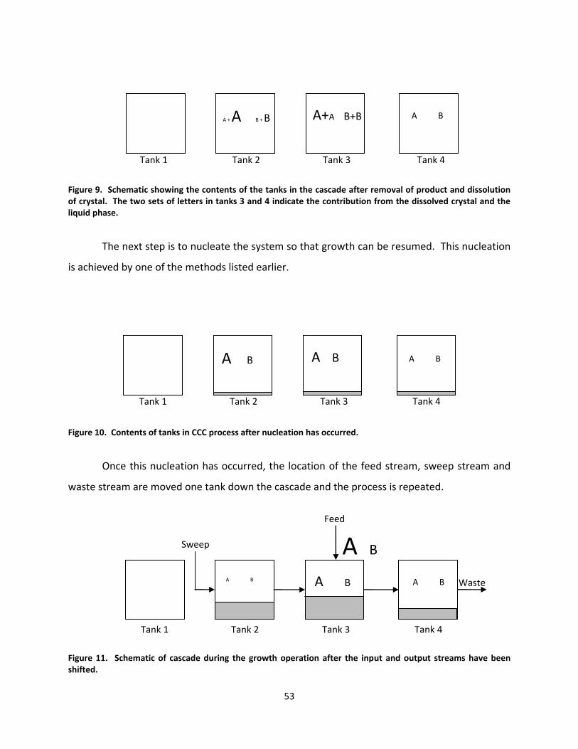
53

Figure 9. Schematic showing the contents of the tanks in the cascade after removal of product and dissolution of crystal. The two sets of letters in tanks 3 and 4 indicate the contribution from the dissolved crystal and the liquid phase.

The next step is to nucleate the system so that growth can be resumed. This nucleation

is achieved by one of the methods listed earlier.

Figure 10. Contents of tanks in CCC process after nucleation has occurred.

Once this nucleation has occurred, the location of the feed stream, sweep stream and

waste stream are moved one tank down the cascade and the process is repeated.

Figure 11. Schematic of cascade during the growth operation after the input and output streams have been shifted.

Feed

Sweep

A B

A B A B

A B


Waste

A B A B A B


A B A + A B + B A+A B+B


54

It was earlier mentioned that there is the possibility for overflow when transferring the

liquid contents after the growth operation. There is also the possibility that tanks will be under-

filled after this transfer operation. If a tank is not full at the beginning of the next growth oper-

ation, the outflow from that tank remains zero until the tank is full, at which point outflow is

resumed.

2.1.2 Alternative Processing Method

The process described above utilized an extra tank for the liquid transfer operation. An

alternative method of operation is to discard the entire liquid contents of the last tank as

waste. The liquid transfer operation as described could then be completed without the need

for an extra tank. The tank from which the product was removed in one cycle becomes the

tank from which the effluent leaves in the next cycle. An overview schematic of this mode of

operation is given in Figure 12.

This implementation of the process without the use of an extra tank is simpler because

it requires less equipment and less liquid transfers. The performance for implementation of

this process with and without an extra tank will be discussed in section 2.4.6.

55

Figure 12. Schematic of process operation when liquid contents of last tank in cascade are discarded. A) Con-tents of each tank at the end of one growth cycle. B) Contents of each tank after the liquid transfer operation. Product has been removed and liquid initially in tank 3 has been discarded. C) Conditions at end of next growth cycle after inlet and outlet points have been moved.

Feed

Waste

Sweep

A B

A B A B

A B

Tank 1 Tank 2 Tank 3

A + A B + B


Feed

Sweep

A B

A B A B

A B


Waste

A+A B+B

A)

B)

C)

56

2.1.3 Operational Similarity to Simulated Moving Bed Chromatography

Although this process seems quite complicated to operate it shares many operational

similarities to simulated moving bed chromatography148. A simulated moving bed is a practical

approximation to a true moving bed process where a separation occurs between a liquid and a

solid phase and both phases move counter-currently to each other. Moving a solid phase is not

a desirable operation and so the simulated moving bed can be used. The proposed crystalliza-

tion operation is not an approximation to an ideal separation process design as a simulated

moving bed is but it is desirable because it provides multiple recrystallizations which give in-

creased purity.

In a simulated moving bed, feed is added continuously to a multi-stage cascade. The

stages are filled with a solid, stationary phase that interacts with the component of interest or

the impurity. The species that interacts with the stationary phase will move more slowly

through the cascade than the other species, leading to separation. To simulate counter-current

operation, the feed and product removal points are periodically shifted in the direction of liquid

flow.

This movement of the flow entry and exit points results in the “movement” of the solid

phase in the opposite direction of the fluid flow. An equivalent process would be to leave the

fluid entry and exit points in place but to move the solid phase one tank in the direction oppo-

site of the fluid flow. This is more difficult than moving the fluid entry and exit points in prac-

tice but it may be simpler to envision the counter-current nature of the process with this de-

scription. A schematic of a simulated moving bed chromatography unit is shown in

Figure 13.

57

Figure 13. Schematic of a simulated moving bed chromatography device. A represents the component of inter-est, B is the impurity and S is the solvent. The block between each inlet/outlet point represents N stages for a 4N stage cascade in total.

The proposed crystallization process is fundamentally different than simulated moving

bed chromatography due to crystallization as the mechanism for separation and the redissolu-

tion of the crystal which allows for multiple recrystallizations but it does share similar operating

principles. The proposed crystallization process can be viewed as the liquid phase moving in

one direction while the crystal moves in the other direction which is similar to the overall result

of the SMB process. The feed and withdrawal points also shift along the length of the cascade

during the course of a cyclical operation and the equipment must be designed to allow for this

to occur. Both the simulated moving bed and the proposed crystallization process will require

significant equipment and control infrastructure in order to carry out the complicated process.

Feed Components: A, B and S

Waste Components: B and S

Sweep Components: S

Product Components: A and S

Direction of Flow

N stages

N stages

N s

tage

s N stages

58

The proposed crystallization process will require some additional equipment that has no

analog in the SMB process. The ability to pump liquid between stages is required in order to

enact the liquid transfer operation which is used to facilitate the recrystallization operations

that increase product purity. Heat transfer equipment to control the temperature of the bulk

liquid in each tank and possibly the temperature at the crystallization surface must also be

present. These are standard, readily available unit operations but the added costs of their con-

struction and operation will need to be considered.

While the simulated moving bed differs significantly from the proposed crystallization

operation because of a different underlying mechanism of separation and the use of batch-like

recrystallization operations, both have similar operational requirements. The complicated na-

ture of the proposed crystallization operation should not immediately disqualify it from consid-

eration although it must be considered when designing separations for a specific application.

2.1.4 Process Discussion

The proposed process has similarities to both a batch crystallization operation and con-

tinuous flow crystallization. The multiple recrystallizations that occur due to the dissolution

and liquid transfer operations are similar to batch recrystallizations while each individual

growth cycle operates as a continuous crystallizer. The benefits of this process are multiple

crystallizations of the component of interest, semi-continuous operation and avoidance of mul-

ti-phase flows. Multiple crystallizations serve to increase the purity of the product while semi-

continuous operation is important for implementation in an overall continuous process and

eliminating multi-phase flows can enhance reliability of the process. The use of a semi-

continuous flow process is important because this process could be implemented in a com-

pletely continuous process if two of these counter-current crystallization operations are run in

parallel. Continuous operation should then be possible with the feed continuously flowing to

one of the two setups.

Multiple recrystallizations are possible due to the use of multiple stages and redissolu-

tion of the crystals after every growth operation. This also allows for smaller supersaturations

to be used in each tank. Supersaturation results from temperature gradients between the bulk

59

liquid and the crystal surface and smaller supersaturations also mean smaller temperature dif-

ferences. This arrangement allows for more economical heat management in addition to the

main benefit of multiple recrystallizations. If crystallization occurs such that higher purity solu-

tions give higher purity crystals then limiting the supersaturation in the first tank will also result

in higher purity product which is the desired outcome. The multiple tanks allow for the yield to

be maintained while getting high crystal purity from a smaller amount of crystallization in the

first tank.

The yield can approach the maximum value through careful selection of the number of

stages and other operating parameters. The yield is limited by how much of species A leaves

the system in the waste stream which is determined by the concentration of A in the final stage

and the flow rate of the waste stream. The concentration in the final stage is limited by the so-

lubility of species A in this stage. This solubility usually decreases with temperature so that the

practical limitation is the lowest feasible operating temperature.

The performance of the proposed process is compared to batch crystallization run to

completion. Batch crystallization is a good comparison because it represents a very common

method of purification and a batch operation run until completion will result in a liquid phase

concentration equal to the equilibrium concentration of species A at the employed tempera-

ture which will give the maximum yield. If this complicated process cannot approach the max-

imum yield while providing higher purity than the batch operation then it will not be worth-

while. A model is first developed for batch crystallization before it is extended to the semi-

continuous process because the batch model is simpler but is readily transferrable to the conti-

nuous process.

In order to maximize yield from the semi-continuous process the concentration in the

final stage and flow rate out of the final stage could be minimized. While the solubility of spe-

cies A may be changed only by changing the temperature, the flow rate of the waste stream

could be lowered in two ways. If some solvent is evaporated between stages after the feed

stage, this will concentrate the stream entering the following stage and decrease the amount of

effluent from that stage. The concentrated stream will have a larger supersaturation driving

force and will deposit more crystal than the original stream.

60

The other option is to recycle some of the waste stream. But in order to recycle, some

of the solvent must first be evaporated. The waste stream is at the lowest possible concentra-

tion of species A (as dictated by the solubility of A) and so adding it directly into the feed stream

will only dilute the feed and lead to worse performance. By evaporating some of the solvent,

the waste stream is concentrated and can be mixed with the feed stream for a possible im-

provement in performance. But the recycling of the waste stream will result in a less pure feed

material that could diminish the overall purity. A good starting point for the amount of solvent

to be evaporated is to match the concentration of species A in the feed and recycle streams.

Either method of decreasing the flow rate requires solvent evaporation which would require a

significant input of energy.

Although the process has been described with the solid crystal being removed as the

product it is possible that a specific chemical system will tend to crystallize the impurity prefe-

rentially to the component of interest. In this situation, the “waste” stream may be enriched in

the component of interest and could be removed as the product. This would be a desirable sit-

uation because the product would already be in liquid form and ready for the next processing

operation but this situation is not expected to be common.

2.2 Batch Modeling

The initial system to be modeled is a batch reactor with three components: the compo-

nent of interest (A), the impurity (B) and the solvent (S). A schematic of the system showing the

important variables is included in Figure 14.

The variables in Figure 14 are defined as follows: mA, mB and mS are the masses (kg) of

species A, B and solvent in the liquid phase respectively; mAc and mBc are the masses (kg) of

each component in the crystal phase; Vl, and Vc are the liquid and crystal phase volumes re-

spectively (m3); CA* and CB

* are the equilibrium liquid phase concentrations; and CAcS and CBc

S

are the surface concentrations of A and B in the solid phases. The total volume of the reactor is

VR. Note that we can define concentrations in the liquid and crystal phases as mj/Vj.

61

Figure 14. Drawing of a batch crystallization tank along with all possible variables for use in deriving equation system for batch crystallization model.

This system has 11 unknowns (mA, mB, ms, mAc, mbc, Vl, Vc, CA*, CB

*, CAc

s and CBcs) Equa-

tions (2.1) through (2.5) are mass balances for the batch system.

*

nA

A A

d mka C C

dt

(2.1)

*

nb

b b b

d mk a C C

dt

(2.2)

0

sd m

dt

(2.3)

Ac Ad m d m

dt dt

(2.4)

bc bd m d m

dt dt

(2.5)

The new variables in the above equations are a, ki and n which are the surface area for

crystal growth, the kinetic incorporation rate constant of species i into the crystal and the ex-

ponential dependence of crystal growth on the supersaturation. These quantities are intro-

duced through the crystal growth mechanism and only a is potentially a controllable parameter.

Values for the parameters ki and n must be measured experimentally because they are chemi-

Vl

mA mB mS

Vc

mAc mBc

CA* CB

*

CAcS CBc

S

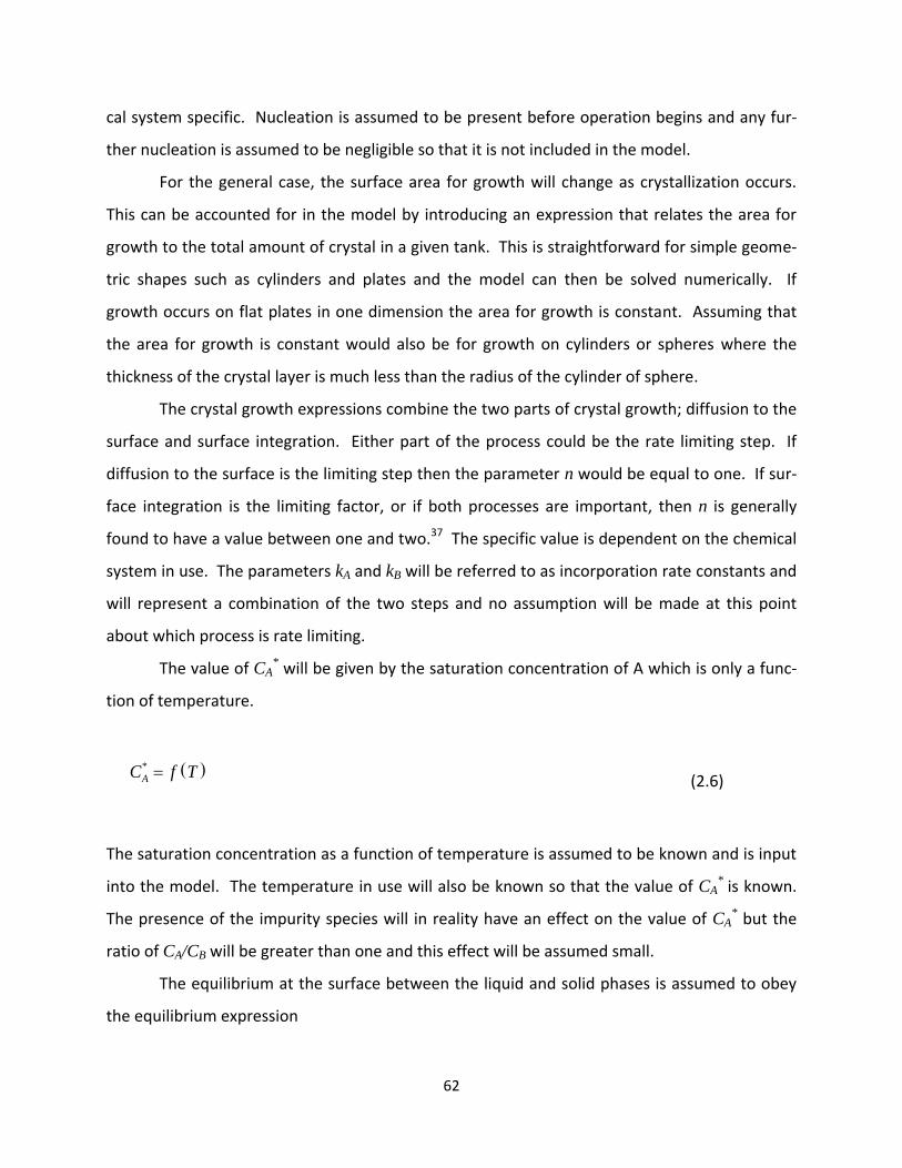
62

cal system specific. Nucleation is assumed to be present before operation begins and any fur-

ther nucleation is assumed to be negligible so that it is not included in the model.

For the general case, the surface area for growth will change as crystallization occurs.

This can be accounted for in the model by introducing an expression that relates the area for

growth to the total amount of crystal in a given tank. This is straightforward for simple geome-

tric shapes such as cylinders and plates and the model can then be solved numerically. If

growth occurs on flat plates in one dimension the area for growth is constant. Assuming that

the area for growth is constant would also be for growth on cylinders or spheres where the

thickness of the crystal layer is much less than the radius of the cylinder of sphere.

The crystal growth expressions combine the two parts of crystal growth; diffusion to the

surface and surface integration. Either part of the process could be the rate limiting step. If

diffusion to the surface is the limiting step then the parameter n would be equal to one. If sur-

face integration is the limiting factor, or if both processes are important, then n is generally

found to have a value between one and two.37 The specific value is dependent on the chemical

system in use. The parameters kA and kB will be referred to as incorporation rate constants and

will represent a combination of the two steps and no assumption will be made at this point

about which process is rate limiting.

The value of CA* will be given by the saturation concentration of A which is only a func-

tion of temperature.

*

AC f T (2.6)

The saturation concentration as a function of temperature is assumed to be known and is input

into the model. The temperature in use will also be known so that the value of CA* is known.

The presence of the impurity species will in reality have an effect on the value of CA* but the

ratio of CA/CB will be greater than one and this effect will be assumed small.

The equilibrium at the surface between the liquid and solid phases is assumed to obey

the equilibrium expression

63

*

*

Ac

s

BcA

s

B

CCK

C C (2.7)

This relationship is similar in form to the separation factor used to measure impurity distribu-

tion in separation of solid solutions by crystallization‡ but instead of relating bulk phase concen-

trations, Equation (2.7) compares equilibrium liquid concentrations to surface solid concentra-

tions.

The parameter K relates changes in equilibrium liquid phase concentrations to changes

in surface solid concentrations which is important for modeling impurity incorporation into the

solid. This parameter will be assumed to only depend on temperature. Because CA* is known

as a function of temperature, K can be used to find the value of the previously unknown para-

meter CB*. Requiring that K be constant is a key assumption of this model.

If a batch experiment were allowed to run for a long time so that complete equilibration

of the solid and liquid occurred, then the value of K could be measured from the bulk proper-

ties of the liquid and solid. Even in this situation, the surface concentration of the solid should

be used for calculating the value of K instead of the average solid concentration. If the crystal

particle size was kept very small during growth and enough time was allowed for solid diffusion

to smooth out any impurity distribution in the solid then the average concentration of the crys-

tals could be used for calculation of K. The average concentration is easier to measure but ex-

perimentally obtaining crystals that are in equilibrium is expected to be difficult and so the sur-

face concentration is a better choice for determination of K.

The ratio of differential crystal growth of species A to species B will be equal to the ratio

of the crystal surface concentration at that time, i.e.

Ac s

Ac

sBc Bc

d mCdt

d m Cdt

(2.8)

‡ See section 1.2.2 and equation (1.21).

64

This equation relates the unknown surface concentrations of the solid to the known growth

rates of the crystal.

The last three equations describe the volumes in the liquid and solid phases.

A A B B s s lm V m V m V V (2.9)

Ac Bcc

c

m m

V

(2.10)

s s

Ac Bc cC C (2.11)

where iV is the partial mass volume of species i and ρc is the density of the crystal.

Equation (2.9) may be simplified for certain systems that form ideal solutions or are di-

lute. If equation cannot be simplified then the partial mass volumes must be known as func-

tions of the composition of the system and temperature. An appropriate activity coefficient

model can be used to find the expressions for partial mass volume.

Equations (2.10) and (2.11) are derived by assuming constant density of the crystal

phase. The constant density of the solid is a good assumption because when dealing with sys-

tems forming solid solutions the A and B species will be very similar chemically. Equation (2.11)

is a special case of equation (2.10) indicating that the surface layer will have the same density

as the bulk of the crystal. This is important because of the use of surface concentration in the

definition of the surface equilibrium constant K.

Assumptions made in developing this model include that the solvent is absent from the

crystal (no inclusions or solid solutions with the component of interest or the impurity) and the

surface equilibrium constant is only a function of temperature. At the beginning of operation

the reactor is full of liquid and a small coating of crystal on a solid surface that will act as a seed

for crystal growth.

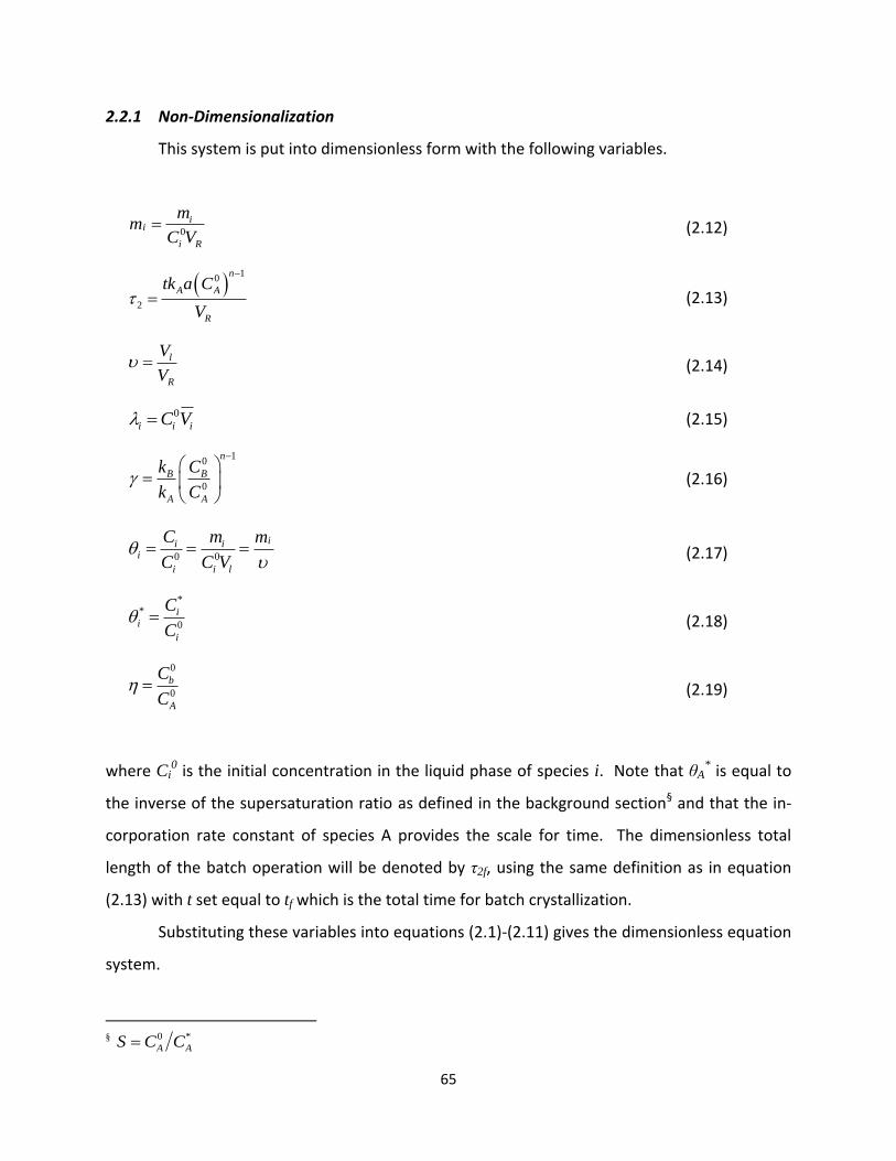
65

2.2.1 Non-Dimensionalization

This system is put into dimensionless form with the following variables.

0

ii

i R

mm

C V (2.12)

1

0

2

n

A A

R

tk a C

V

(2.13)

l

R

V

V (2.14)

0

i i iC V (2.15)

10

0

n

B B

A A

k C

k C

(2.16)

0 0

ii ii

i i l

C m m

C C V

(2.17)

**

0

ii

i

C

C (2.18)

0

0

b

A

C

C (2.19)

where Ci0 is the initial concentration in the liquid phase of species i. Note that θA

* is equal to

the inverse of the supersaturation ratio as defined in the background section§ and that the in-

corporation rate constant of species A provides the scale for time. The dimensionless total

length of the batch operation will be denoted by τ2f, using the same definition as in equation

(2.13) with t set equal to tf which is the total time for batch crystallization.

Substituting these variables into equations (2.1)-(2.11) gives the dimensionless equation

system.

§

0 *

A AS C C

66

*

2

A n

A A

d m

d

(2.20)

*

2

B n

B B

d m

d

(2.21)

2

0sd m

d

(2.22)

2 2

Ac Ad m d m

d d

(2.23)

2 2

Bc Bd m d m

d d

(2.24)

*

A f T (2.25)

*

*

Ac

s

BcA

s

B

K

(2.26)

2

2

Ac

s

Ac

sBc Bc

d m

d

d m

d

(2.27)

A B sA B sm m m (2.28)

Ac Bc c cm m (2.29)

s s

cAc Bc (2.30)

2.2.2 Batch Model Analysis

It will also be assumed for the following analysis that the liquid volume is constant (di-

lute system), the temperature is constant and the parameter n is equal to one. Note that the

initial condition Vl0=VR and the assumption that liquid volume is constant implies that Vl=VR.

Under this assumption i im . Constant temperature means that K and θA* are constant be-

cause both K and θA* have been assumed to depend only on temperature. These assumptions

67

limit this model to systems with low saturation concentrations and low supersaturations but

allow the development of closed form analytical solutions.

Under these assumptions equation (2.20) becomes:

*

2

A

A A

d

d

(2.31)

This can be solved directly for θA recalling that the initial concentration in dimensionless form is

1 by definition.

2* *

2 1A A A e (2.32)

In order to solve for θB, an expression for θB* is required. First combine equations (2.23),

(2.24) and (2.27) to give equation (2.33).

*

2 2 2

*

22 2

Ac AA

sA AAc

sBc B BBc B B

d m d m dd d d

dd m d mdd d

(2.33)

Then combine equations (2.33) and (2.26) and solve for θB* to give equation (2.34).

**

* *

A BB

A A AK

(2.34)

A solvable differential equation for θB is then given by combining equations (2.21), (2.32) and

(2.34). This is presented in equation (2.35).

68

22

*

11 1

b BB

A

d

d Ke

(2.35)

The initial condition by definition is θB0=1 and the solution to equation (2.35) is given in

equation (2.36).

2

*

*

11 1

11 1

A

B

A

Ke

K

(2.36)

These expressions for the liquid phase concentrations will be useful during the analysis

of the model for the semi-continuous process.

2.2.3 Discussion of Impurity Concentration when γ>>1

When γ is very large, equation (2.34) indicates that the critical concentration of the im-

purity in the liquid becomes equal to the concentration of the impurity in the liquid.

**

* *lim lim A B

B B

A A AK

(2.37)

This expression also requires that γ<<K.

This result indicates that when γ is very large there is no resistance to incorporation of

the impurity into the solid. γ is the ratio of incorporation rate constants and it will be much

greater than one when the incorporation rate constant of the impurity is much greater than the

incorporation rate constant of the component of interest.

69

In this situation the only limitation to impurity addition to the solid phase will be the

amount of solid phase present which is controlled by the growth of species A. Impurity will be

added to the crystal as soon as the crystal is grown. This means that concentration change in B

will have the same time constant as the concentration profile for A. The amount of change in

the concentration of B can be different than the change in A but the time scales over which the

concentration changes occur will be the same.

2.3 CCC Modeling

A model of the semi-continuous process described in section 2.1 was developed in order

to estimate the possible benefits of this process and to provide guidance for experimentation.

The equations needed to model the semi-continuous process are very similar to the equations

that describe batch crystallization.

The following set of equations will be derived for a single tank. These equations can be

applied to any number of tanks to give the full equation system for a multi-tank process. The

system is shown in Figure 15.

Figure 15. Drawing of one tank along with all possible variables for use in deriving equation system for counter-current crystallization model.

F

CAf CB

f CSf

Q

CA CB Cs

Vl

mA mB mS

Vc

mAc mBc

P

CAP CB

P

CSP

CA* CB

*

CAcS CBc

S

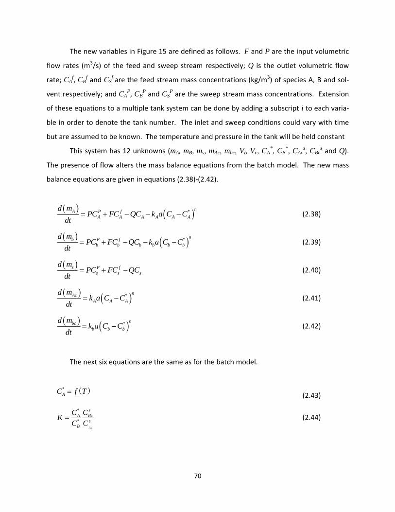
70

The new variables in Figure 15 are defined as follows. F and P are the input volumetric

flow rates (m3/s) of the feed and sweep stream respectively; Q is the outlet volumetric flow

rate; CAf, CB

f and CSf are the feed stream mass concentrations (kg/m3) of species A, B and sol-

vent respectively; and CAP, CB

P and CSP are the sweep stream mass concentrations. Extension

of these equations to a multiple tank system can be done by adding a subscript i to each varia-

ble in order to denote the tank number. The inlet and sweep conditions could vary with time

but are assumed to be known. The temperature and pressure in the tank will be held constant

This system has 12 unknowns (mA, mB, ms, mAc, mbc, Vl, Vc, CA*, CB

*, CAc

s, CBc

s and Q).

The presence of flow alters the mass balance equations from the batch model. The new mass

balance equations are given in equations (2.38)-(2.42).

*

nA P f

A A A A A A

d mPC FC QC k a C C

dt (2.38)

*

nb P f

b b b b b b

d mPC FC QC k a C C

dt (2.39)

s P f

s s s

d mPC FC QC

dt (2.40)

*

nAc

A A A

d mk a C C

dt (2.41)

*

nbc

b b b

d mk a C C

dt (2.42)

The next six equations are the same as for the batch model.

*

AC f T (2.43)

*

*

Ac

s

BcA

s

B

CCK

C C (2.44)

71

Ac s

Ac

sBc Bc

d mCdt

d m Cdt

(2.45)

A A B B s s lm V m V m V V (2.46)

Ac Bcc

c

m m

V

(2.47)

s s

Ac Bc cC C (2.48)

A new equation is needed because of flow through the cascade and it relates to the op-

eration of the system. The chosen constraint will be that the total volume in the reactor (Vl +

Vc) is constant. Alternatively, an assumption about the solid phase volume, liquid phase vo-

lume or outlet flow rate could be made.

R l cV V V (2.49)

This volume is the volume for a single tank. A cascade of N reactors would have a total volume

equal to NVR.

2.3.1 Non-Dimensionalization

The model equations were non-dimensionalized using the following dimensionless va-

riables.

0

ii

i R

mm

C V (2.50)

R

tF

V (2.51)

l

R

V

V (2.52)

72

0

i i iC V (2.53)

1

0n

i i

i

k a C

F

(2.54)

10

0

n

B B B

A A A

k C

k C

(2.55)

0 0

ii ii

i i l

C m m

C C V

(2.56)

**

0

ii

i

C

C

(2.57)

P

F (2.58)

Q

F (2.59)

0

cc

AC

(2.60)

0

0

b

A

C

C (2.61)

The difference from the batch equations is that the time is now non-dimensionalized using the

feed flow rate instead of the incorporation rate constant of A. The dimensionless time in the

flow system is denoted as τ as opposed to τ2 in the batch system. The dimensionless total

length of the growth operation will be denoted by τf, using the same definition as in equation

(2.51) with t set equal to tf which is the total time for growth.

These variables when inserted into equations (2.38)-(2.49) give the following dimension-

less system of equations.

*

A nP f

A A A A A A

d m

d

(2.62)

73

*

B nP f

B B B B B B

d m

d

(2.63)

sP f

s s s

d m

d

(2.64)

*

Ac n

A A A

d m

d

(2.65)

*

Bc n

B B B

d m

d

(2.66)

*

A f T (2.67)

*

*

B Ac

s

BcA

sK

(2.68)

Acs

Ac

sBc Bc

d m

d

d m

d

(2.69)

A B sA B sm m m (2.70)

Ac Bc c cm m (2.71)

s s

cAc Bc (2.72)

1 c (2.73)

This system of equations was solved using MATLAB. Starting from an arbitrary initial

state the simulation is repeated for many cycles of operation until the concentrations in each

tank at the beginning of one growth operation are the same as at the beginning of the next

growth operation. This condition is referred to as cyclical steady state.

The mole fraction of the impurity in the solid at the surface is given by equation (2.74).

74

0 0

0 0

1 1

1 1

ss BcBc s ss s

Ac AcA BBc Ac

s s

A B Bc Bc

Cx

C C CC C

C C C

(2.74)

where η is the ratio of the initial concentrations of species B to species A as defined in equation

(2.61). Once a layer of crystal is deposited, its concentration is assumed constant on the time

scale of this process so the value of xBcs as a function of time will give the concentration profile

of the crystal as a function of time. The value of this mole fraction can be calculated from the

solution to the above set of equations.

2.3.2 Analytical Solution for Yield in Three Stage Cascade

An analytical expression for the yield at cyclic steady state from this process was devel-

oped for a three stage cascade with feed at stage two and a sweep stream at stage 1. This is

the smallest number of stages able to capture all of the possible advantages of the proposed

counter-current crystallization. It was also assumed for this analysis that the temperature in

every stage was the same, the parameter n is equal to one, crystal growth only occurs in one

planar dimension so that the area for crystal growth is constant and that the system is dilute in

A and B so that the liquid volume remains constant. The expression for yield was generated via

a stage by stage calculation. It is straightforward to extend this analysis to a system with more

stages but the algebra required is significant.

The expression for the yield of a three stage cascade with feed at stage two and a sweep

stream is given in equation (2.75). A full derivation of this quantity is included in section 6.2.

75

**0

tank 1

**0

*

2

tank 2

**0

*

*

1

1

1

1 1

1

11

1

AA

A

AA

A

A

A

AA

A A A

AA

A

A

A

A

A

y

2

tank 3

11 1

1 1 1

AA A

A A A A A

(2.75)

Equation (2.75) can be simplified to give the expression for yield from a two stage cas-

cade with feed at stage 1 by setting the sweep stream flow rate to zero. This follows from the

sequential nature of the process. A downstream tank is only affected by its nearest neighbor

tank in the upstream direction. Setting the sweep flow rate equal to zero results in no outflow

from tank one and therefore no input into tank two. It will not be necessary to study this spe-

cial case because a more general analysis will cover the interesting details of this solution.

Analysis of this solution will be facilitated by looking at the individual yield in each of the

three tanks if a single growth operation were run until steady state is achieved in each stage.

The expressions for the yield from the three tanks in this situation are given in equations (2.76)-

(2.78)

**0

ss,tank 1A

A

A

y

(2.76)

76

**0

*

ss,tank 2

1

1

AA

A

A

A

y

(2.77)

**0

*

*

ss,tank 3

1

11

1

AA

A

A

A

A

A

y

(2.78)

Equations (2.75)-(2.78) show that the yield of the counter-current crystallization process

at cyclical steady given in equation (2.75) is a weighted sum of the yield from each tank during a

single growth phase run until steady state is achieved. The weight on tank 1 is 1 while the

weights on the other tanks in the cascade are functions of the dimensionless sweep flow rate ψ

and the dimensionless reaction rate βA. If the sweep flow rate is set to zero the weighting factor

on tank two yield will become one. The weighting factor on the first tank in any cascade will be

one because that is the tank from which the product is removed.

The weighting factor for each tank is composed of the weighting factor from the adja-

cent upstream tank multiplied by an additional unique factor. The weighting factor for the

second/feed tank is more complicated that the unique portion of the weighting factor from the

third tank. The presence of input streams is seen to result in more complicated weighting fac-

tors.

The values of the weighting factors in any tank except tank 1 are strictly less than or

equal to one. This indicates that the proposed cyclical process can at best match the yield for a

single growth operation run until steady state is achieved if the crystal is collected from all

tanks but will likely have worse yield than a single pass operation with recovery from every

tank.

Another important point to be gleaned is that the operating time for the growth phase

of the counter-current crystallization operation does not affect the cyclical steady state yield

under these conditions. Equation (2.75) was generated using the full transient equation system

and all terms involving time cancelled out when solving for the yield. As long as the process is

77

run until cyclical steady state is achieved the duration of each individual growth cycle does not

matter. The effect of varying total growth times on the process will be to change the number of

cycles necessary to achieve cyclical steady state with shorter growth times requiring more

cycles until steady state.

This conclusion is dependent on the assumption used in the derivation of the yield that

the liquid volume remains constant. This assumption means that only a small amount of

growth can occur because the simulation constrains the sum of liquid and solid volume to be

constant. Even in dilute systems a large amount of crystal can be grown if the cascade is oper-

ated for long times. This expression for the yield is limited to short operating times and the ef-

fect of longer operating times for appreciable crystal growth is discussed below along with the

results from the full simulation.

The sweep tank (tank 1) will always decrease overall yield unless the sweep stream con-

centration is greater than or equal to the saturation concentration. The intended purpose of

the sweep stream is to increase the purity of the final product and this expression indicates that

any increase in purity will come at a cost of yield unless the sweep stream is highly concen-

trated in species A. The effect of the sweep stream flow rate and concentration on product

purity is analyzed using MATLAB simulations because an analytical solution for the purity was

not obtained.

Excessively high sweep stream flow rates can result in zero net crystal growth in tank 1.

The product is the crystal formed in tank 1 of the cascade so the sweep stream must be low

enough to allow net crystal growth to occur in tank 1. Conditions for which there is no crystal

growth in tank 1 were not studied. The sweep stream flow rate can be so high as to eliminate

growth in tank 1 while still allowing growth in tanks 2 and 3 but this situation is not important

because no product can be removed if there is no growth in tank 1.

Examination of equations (2.76)-(2.78) also shows that the yield from each tank after

the feed is less than that from the immediately preceding tank. Adding more tanks in order to

increase yield then is subject to diminishing returns. Multiple tanks do increase the overall

yield but small increases in yield must be balanced against the increase in equipment and oper-

ating costs to perform the cyclical counter current crystallization process in a large cascade.

78

This analysis was performed under the assumption that the temperature in each stage

was constant. Constant temperature also implies that βA is the same in each stage. Moving to

a system with different temperature in each stage would complicate the algebra but the same

types of relationship would be expected. The main difference would be that instead of only βA

appearing in the equations, there would be a βA,i for every stage. This modification is not ex-

pected to change the preceding analysis.

2.3.3 Analytical Purity for Certain Values of the System Specific Parameters

The concentration profile of the impurity cannot be solved for analytically in general us-

ing the equation system outlined in section 2.3. But for limited values of the system specific

parameters γ and K analytical solutions can be determined. The concentration profile of the

impurity can be determined when γ<<1 or when γ>>1 and K<<1 with an arbitrary number of

stages with or without a sweep stream.

While solutions are possible for large cascades, a one stage system was used because

the results become quite complicated with multiple stages and are difficult to analyze. The de-

rivation of the concentration profiles for this system is discussed in appendix 6.3. A one stage

system can provide insight that can inform further study using numerical simulations. The use

of a sweep stream with the one stage system is done only to provide insight on the effect of a

sweep stream when longer cascades are used. A sweep stream would not be employed in prac-

tice with a one stage system.

The availability of an analytical impurity concentration profile allows an analytical ex-

pression for the purity to be determined. The purity and yield for the one stage system with a

sweep stream at cyclical steady state is given in the following equations for both situations.

When γ<<1 the purity is given by

*

*

1

11

11 1 1

1

B

B AA

A

p

K

(2.79)

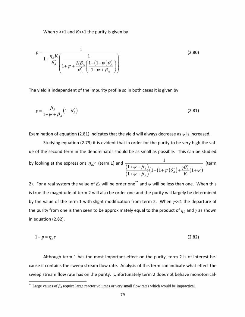
79

When γ >>1 and K<<1 the purity is given by

* *

*

1

11

1 11

1

B

A AA

A A

pK

K

(2.80)

The yield is independent of the impurity profile so in both cases it is given by

*11

AA

A

y

(2.81)

Examination of equation (2.81) indicates that the yield will always decrease as ψ is increased.

Studying equation (2.79) it is evident that in order for the purity to be very high the val-

ue of the second term in the denominator should be as small as possible. This can be studied

by looking at the expressions B (term 1) and

*

*

1

11 1 1

1

B AA

A K

(term

2). For a real system the value of βA will be order one** and ψ will be less than one. When this

is true the magnitude of term 2 will also be order one and the purity will largely be determined

by the value of the term 1 with slight modification from term 2. When γ<<1 the departure of

the purity from one is then seen to be approximately equal to the product of ηB and γ as shown

in equation (2.82).

1 Bp (2.82)

Although term 1 has the most important effect on the purity, term 2 is of interest be-

cause it contains the sweep stream flow rate. Analysis of this term can indicate what effect the

sweep stream flow rate has on the purity. Unfortunately term 2 does not behave monotonical-

** Large values of βA require large reactor volumes or very small flow rates which would be impractical.

80

ly for all parameter values. No simple analysis is possible but once the relevant system specific

parameters are known equation (2.79) could be used to understand how the operating parame-

ters impact the purity from this process.

A more instructive analysis can be performed on equation (2.80) for the situation when

γ >>1 and K <<1. Purity will be higher when the second term in the denominator is as small as

possible. The expression determining the purity now consists of two terms: *

B

A

K

(term 3)

and

*

*

1

1 11

1

AA

A A

K

(term 4). The value of term 3 is controlled by the product of ηB

and K while term 4 will be order one for the parameter values expected for a practical system.

This indicates that the departure of the purity from one when γ >>1 and K <<1 is roughly de-

termined by the product of ηB and K as shown in equation (2.83).

1 Bp K (2.83)

To understand the effect of the sweep stream flow rate on the purity in this situation,

term 4 is compared to its value at ψ=0. The equality will again be assumed so that increasing ψ

gives a decreasing value for this term.

* *

* *

1 1

1 1 11 1

1 1

A A AA

A A A A

K K

(2.84)

This can be rearranged to give

*

*

11 1

1

A AA

A A

K

(2.85)

81

If this equality is satisfied then the purity will increase with increasing sweep stream flow rate.

If the right hand side of the equality in equation (2.85) is less than zero then any value of the

sweep stream flow rate greater than zero will give increased purity. Assuming this is the case

and performing some rearrangement gives

*

*

11 1 0

1

A AA

A A

K

(2.86)

2*

*

1

1 1

A A

A A A

K

(2.87)

*

2* *

11

1 1

A AA

A A A AK

(2.88)

Recall that θA* is order one and note that ratio of βA/(1+ βA) or βA /(1+ βA)2 will always be

between zero and 1 for βA>0. This means the right hand side of equation (2.88) will always be

order 1. K was constrained at the beginning of the derivation to be much less than one so that

1/K will be much greater than one and therefore equality (2.88) is true. This means that equali-

ty (2.86) is also true and increasing ψ will result in increased purity when K<<1 and γ>>1.

The analysis in this section has shown that in situations where γ<<1 or when K<<1 and

γ>>1 the departure of the purity from unity is approximately given by the product of ηB and γ or

the product of ηB and K respectively for a one stage system. Higher purities will result from

lower system specific parameter values (γ and K) and lower values of the initial concentration

ratio of the impurity to the component of interest (ηB). These parameters will often be fixed by

the specific chemical system and a given feed stream concentration but systems with lower

values of these parameters will result in higher purity products.

The intended purpose of the sweep stream was to increase product purity and this is

seen to be the case under certain conditions although the magnitude of this effect is expected

to be small in practical systems (βA order one and ψ order one or less). Also recall that the yield

always decreases with increasing sweep stream flow rate. A more general analysis of the effect

82

of different parameters on the purity will be done using the numerical solution to the full model

in section 2.4.

2.3.4 General Model Comments

The major assumptions made in this model are the temperature dependent equilibrium

relationship at the surface and the expressions for crystal growth. These expressions govern

the incorporation of the impurity into the crystal and if they are not reasonable then the results

will not be useful. Experimentation is required in order to determine how valid these assump-

tions are and to provide guidance for better functional forms if these are not appropriate.

Another assumption is that temperature in each tank and at the crystallization surface

can be held constant. Depending on the amount of crystallization occurring and the size of

each tank heat transfer limitations could be important. This is an important consideration

when designing the process equipment which may dictate a particular cooling method.

This model does not assume dilute solutions. It accounts for variable liquid phase vo-

lumes for systems with high concentrations in the liquid phase. Issues with the liquid transfer

operation such as under and overfilling are only expected to apply in concentrated systems so

that operation of dilute systems will be less complicated in terms of operational programming.

2.4 CCC Model Results

The physical parameter values and variable ranges used in the model simulation are

shown in Table 1 and are based on published physical properties of asparagines.149, 150 The rea-

son for the use of asparagine properties will be discussed in section 4.2.3 when the model ex-

perimental system is discussed but for now it is only necessary to note that the density is in a

common range for small molecule solids150 and the solubility varies strongly with temperature

in the vicinity of room temperature. The mass specific volumes for A and B are at infinite dilu-

tion because the solubility of asparagine in water is low. A and B will have very similar struc-

tures in solid-solution-forming systems so the mass specific volume of the impurity will be as-

sumed to be the same as for species A.

83

Parameter Value(s) Operational Variable

Range of Values

CA* 7.4x10-5e.04*T g/kg solvent (T in Kelvin) ψ 0-1

ρC 1543 kg/m3 βA 0.1-100

VA0=VB

0 6x10-4 m3/kg K 0.1-10

Vs0 0.001 m3/kg γ 0.1-10

τ 3

T 273.15 K

n 1

CA0 25 kg/m3

CB0 2 kg/m3

Table 1. Parameters values and variable ranges used for MATLAB simulation of semi-continuous counter current crystallization process.

The value of the parameter n is assumed to be one and growth is assumed to occur in

only one dimension. Planar one-dimensional growth allows the area a to be constant so that βA

is only dependent on the feed stream flow rate. Assuming that n is one will be valid in systems

operated at high supersaturations and for systems with microscopically rough surface as dis-

cussed in section 1.1.2. The roughness of the surface of a growing crystal is a property of the

specific chemical undergoing growth and must be determined for each unique system.

The use of a dilute system allows equation (2.46) to be simplified. Instead of using par-

tial mass volumes for A, B and the solvent the mass specific volume at infinite dilution can be

used for A and B and the pure component specific volume can be used for the solvent. This

simplification removes the need to find a relationship for the partial mass volumes as a function

of the concentration of all species.

The concentration profiles for species A and B in each stage of a three stage cascade

with feed at stage two are shown in Figure 16, Figure 17 and Figure 18. The system and opera-

tional parameters in these figures are K=0.5, γ=0.5, ψ=0.1, βA=2, τf=2 and T=273.15 K. Note that

the concentration of each species is normalized to the feed concentration of that species so

84

that the dimensionless concentration of B can be greater than the dimensionless concentration

of A even though the actual concentration of A is always higher than B.

These figures show a process occurring with a time constant for θA of roughly 0.5. The

time constant for flow-dependent phenomena in tanks 2 and 3 should be approximately one

because of the definition of τ and in tank 1 it should be 10 because the sweep stream flow rate

is set to 0.1. However, if this was a batch operation the time constant for θA would instead be

given by 1/βA. This represents the time constant for crystallization which in this case is 0.5. The

growth cycle is therefore seen to be dominated by crystallization and behave very much like

batch crystallization over the initial period of time. For the impurity, the time constant in the

first tank is approximately 1. This is the expected result with γ equal to 0.5 and βA equal to 2.

This means that the crystallization and flow time constant for the impurity in tanks 2 and 3 are

nearly equal. The observed time constant in tanks 2 and 3 are slightly shorter than in tank 1

because the flow rate is much higher allowing some depletion to occur by flow out of the stage

in addition to depletion by crystallization.

If the growth cycle is operated for a long period of time, the steady state profile will be

achieved and further deposition will be at constant rate and composition. Operating for very

long times will result in the average composition of the crystal being controlled by the steady

state deposition with the initial transient representing a very small fraction of the total crystal.

These figures demonstrate that the continuous process is controlled by the fastest time

constant of the system. The competing time constants are proportional to 1/βA and 1/(1+ ψ).

When βA is greater than 1+ψ the reaction time constant will be much smaller than the flow time

constant and the concentration decrease is controlled by crystallization.

85

Figure 16. Dimensionless concentration plots for stage 1 vs. time over one growth cycle after cyclic steady state has been achieved in the semi-continuous process. Simulated process is 3 stages with feed at stage 2 with K=0.5, γ=0.5, ψ=0.1, βA=2, τf=2 and T=273.15 K


0

0.2

0.4

0.6

0.8

1

1.2

1.4

1.6

0 0.5 1 1.5 2

Dim

ensi

on

less

Con

cen

trati

on

τ

0

0.2

0.4

0.6

0.8

1

1.2

1.4

1.6

0 0.5 1 1.5 2

Dim

ensi

on

less

Con

cen

trati

on

τ

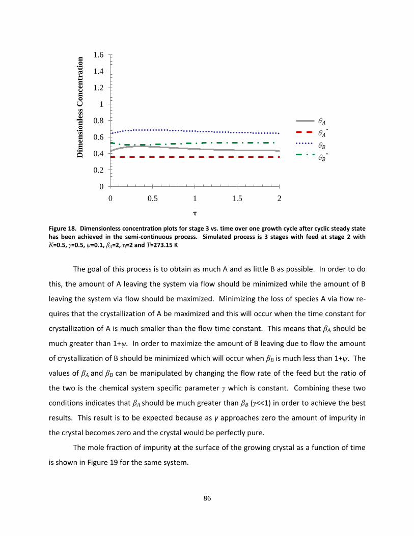
86


The goal of this process is to obtain as much A and as little B as possible. In order to do

this, the amount of A leaving the system via flow should be minimized while the amount of B

leaving the system via flow should be maximized. Minimizing the loss of species A via flow re-

quires that the crystallization of A be maximized and this will occur when the time constant for

crystallization of A is much smaller than the flow time constant. This means that βA should be

much greater than 1+ψ. In order to maximize the amount of B leaving due to flow the amount

of crystallization of B should be minimized which will occur when βB is much less than 1+ψ. The

values of βA and βB can be manipulated by changing the flow rate of the feed but the ratio of

the two is the chemical system specific parameter γ which is constant. Combining these two

conditions indicates that βA should be much greater than βB (γ<<1) in order to achieve the best

results. This result is to be expected because as γ approaches zero the amount of impurity in

the crystal becomes zero and the crystal would be perfectly pure.

The mole fraction of impurity at the surface of the growing crystal as a function of time

is shown in Figure 19 for the same system.

0

0.2

0.4

0.6

0.8

1

1.2

1.4

1.6

0 0.5 1 1.5 2

Dim

ensi

on

less

Con

cen

trati

on

τ

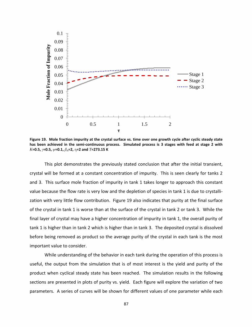
87

Figure 19. Mole fraction impurity at the crystal surface vs. time over one growth cycle after cyclic steady state has been achieved in the semi-continuous process. Simulated process is 3 stages with feed at stage 2 with K=0.5, γ=0.5, ψ=0.1, βA=2, τf=2 and T=273.15 K

This plot demonstrates the previously stated conclusion that after the initial transient,

crystal will be formed at a constant concentration of impurity. This is seen clearly for tanks 2

and 3. This surface mole fraction of impurity in tank 1 takes longer to approach this constant

value because the flow rate is very low and the depletion of species in tank 1 is due to crystalli-

zation with very little flow contribution. Figure 19 also indicates that purity at the final surface

of the crystal in tank 1 is worse than at the surface of the crystal in tank 2 or tank 3. While the

final layer of crystal may have a higher concentration of impurity in tank 1, the overall purity of

tank 1 is higher than in tank 2 which is higher than in tank 3. The deposited crystal is dissolved

before being removed as product so the average purity of the crystal in each tank is the most

important value to consider.

While understanding of the behavior in each tank during the operation of this process is

useful, the output from the simulation that is of most interest is the yield and purity of the

product when cyclical steady state has been reached. The simulation results in the following

sections are presented in plots of purity vs. yield. Each figure will explore the variation of two

parameters. A series of curves will be shown for different values of one parameter while each

0

0.01

0.02

0.03

0.04

0.05

0.06

0.07

0.08

0.09

0.1

0 0.5 1 1.5 2

Mole

Fra

ctio

n o

f Im

pu

rity

τ

Stage 1

Stage 2

Stage 3

88

individual line will consist of multiple simulations done while varying a second parameter. Each

point on an individual line will correspond to one simulation calculation with a unique set of

values for the parameters. Note that the purity of the feed solution on a solvent free basis used

in all simulations is 0.9259.

One of the goals of this process is to provide better performance than a batch opera-

tion, assessed by comparison of the yield and purity from a batch crystallization run to comple-

tion to those of the cyclical steady state of the counter current process. A batch crystallization

run until completion will give the best possible yield for a given set of operating conditions and

the proposed counter current process cannot exceed this yield. Better performance will be in-

dicated by close approach to the batch yield but with purity higher than for batch crystalliza-

tion.

Comparisons of the batch model to the semi-continuous process model will be made

only when the chemical system specific parameters (K, γ and n) are constant. Changing these

values changes the batch performance and so a clear comparison is not possible. Study of the

variation of the chemical system specific parameters is done to understand the different opera-

tional regimes and not to determine optimal values. K, γ and n are dictated by the specific

chemical system in use and cannot be varied at will. Batch comparisons will be made when va-

rying controllable operating parameters such as flow rates and times.

89

2.4.1 Effect of the chemical system parameters K and γ

2.4.1.1 Effects of varying γ

Figure 20. Plot of purity vs. yield when βA is varied at various values of the constant ratio γ. τf=2, ψ=0, 3 stages, feed at stage 1, K=0.5, and T=273.15 K. βA varies from 0.1 to 30 moving left to right in each individual line. Ver-tical dotted lines represent constant values of βA and individual points correspond to the batch comparison points for different values of γ. The purity of the feed solution is 0.9259.

Figure 20 shows that the value of γ has a significant impact on the performance of the

counter-current crystallization process. In all cases the yield increases as the value of βA, the

incorporation rate constant of species A, increases. Higher incorporation rate constants result

in higher yields. For γ less than unity, the purity decreases as βA increases while for γ greater

than one the purity increases as the yield increases. When γ is equal than unity, there is no

change in purity as the incorporation rate constant of A increases.

When the incorporation rate constant of B is faster than A (γ>1), the purity of the prod-

uct is decreased as βA increases. Conversely, when B is added to the crystal at a slower rate

than A (γ<1) the product will become more pure as βA increases. At a given value of βA the pur-

ity increases as γ approaches zero. This is in line with the definition of γ which indicates that

0.90

0.91

0.92

0.93

0.94

0.95

0.96

0.97

0.98

0.99

1.00

0 0.1 0.2 0.3 0.4 0.5 0.6 0.7

Pu

rity

Yield

γ=0.1

γ=0.5

γ=1

γ=2

γ=10

Batch γ=0.1

Batch γ=0.5

Batch γ=1

Batch γ=2

Batch γ=10

β=2.8 β=0.6 β=0.1

90

when γ=0 the incorporation rate of B into the crystal is zero and therefore the product would be

perfectly pure.

As βA becomes very high the product from the counter-current crystallization approach-

es the same final yield and purity for all values of γ. βA decreases with flow rate but increases

with the intrinsic incorporation rate constants and surface area for growth. As βA becomes

larger the conditions in each tank are less and less affected by kinetic considerations and the

yield and purity approach a value independent of γ. The final purity is then determined by

thermodynamic factors which in this model are represented by K and θA*.

2.4.1.2 Analysis of Behavior at γ=1

Figure 20 indicates that the purity does not change when βA changes if γ=1. The ratio of

driving forces is given by

*

*

A A

B B

(2.89)

A plot of the ratio of driving forces for crystallization in tank 1 is presented in Figure 21 for γ

equal to 0.5, 1 and 2.

The ratio of the driving forces is constant and independent of βA only when γ =1. The

driving force for the impurity, θB-θB*, is determined by the parameters, γ, K, τf and Ca* but Fig-

ure 21 indicates that it is directly proportional to θA-θA* when γ =1. By combining equations

(2.33) and (2.26) the ratio of driving forces can also be represented as

* *

* *

A A B

B B A

K

(2.90)

Recall that K, γ and θA* are all constant at constant temperature indicating that a constant ratio

of driving forces is equivalent to a constant value of θB* in this model.

91

Figure 21. Plots of the ratio of crystallization driving forces for A and B in stage 1 vs. τ for βA=2. τf=2, ψ=0, 3 stag-es, feed at stage 1, K=0.5, and T=273.15 K. γ is 2 for the top line, 1 for the middle line and 0.5 for the lower line.

This can be understood in the batch case making use of the analytical expressions for

liquid phase concentration developed in section 2.2.2.

2

2

*

*

*

*

* *

11 1

11 1

11 1 1

A

ABB

A A

A A

Ke

K

K Ke

(2.91)

When γ=1 the following result is obtained.

*

*

1

11 1

B

A

K

(2.92)

This expression is constant when temperature is constant which results in constant purity.

0.50

1.00

1.50

2.00

2.50

3.00

0 0.5 1 1.5 2

Dri

vin

g F

orc

e R

ati

o

τ

γ=1

γ=0.5

γ=2

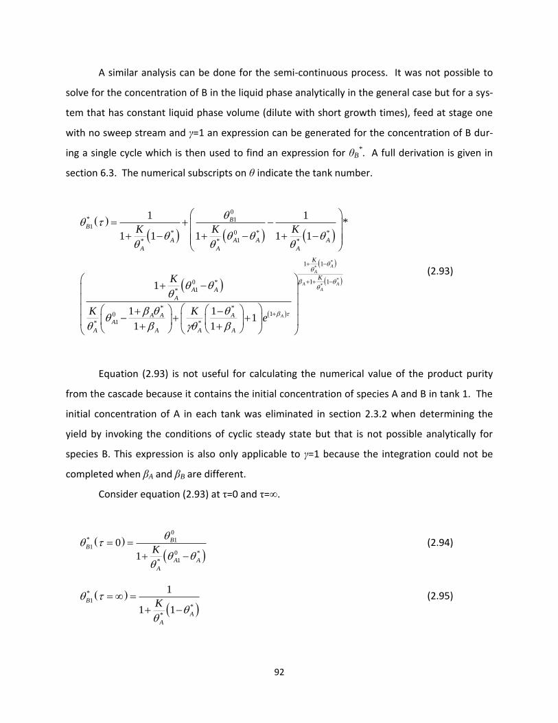
92

A similar analysis can be done for the semi-continuous process. It was not possible to

solve for the concentration of B in the liquid phase analytically in the general case but for a sys-

tem that has constant liquid phase volume (dilute with short growth times), feed at stage one

with no sweep stream and γ=1 an expression can be generated for the concentration of B dur-

ing a single cycle which is then used to find an expression for θB*. A full derivation is given in

section 6.3. The numerical subscripts on θ indicate the tank number.

*

*

*

*

0* 11

* 0 * *

1* * *

1 1

1 10 *

1*

* *10

1* *

1 1*

1 1 1 1 1

1

1 11

1 1

A

A

A A

A

A

BB

A A A A

A A A

K

K

A A

A

A A AA

A A A A

K K K

K

K Ke

(2.93)

Equation (2.93) is not useful for calculating the numerical value of the product purity

from the cascade because it contains the initial concentration of species A and B in tank 1. The

initial concentration of A in each tank was eliminated in section 2.3.2 when determining the

yield by invoking the conditions of cyclic steady state but that is not possible analytically for

species B. This expression is also only applicable to γ=1 because the integration could not be

completed when βA and βB are different.

Consider equation (2.93) at τ=0 and τ=∞.

0* 11

0 *

1*

0

1

BB

A A

A

K

(2.94)

*

1*

*

1

1 1B

A

A

K

(2.95)

93

This result matches the batch result given in equation (2.92) at long times and also at all times if

θA10 and θB1

0 are equal to 1. The values of θA10 and θB1

0 will always be order one because they

are normalized but even small differences from unity will be important for very small values of

K. Very large values of K will result in θB1* approaching zero so that very little absolute change

will be observed and this amount of change will be negligible in relation to the initial driving

force.

The difference between the value of θB1* at τ=0 and τ=∞ gives the maximum amount of

change in θB1* for a given set of parameters. This is true because the term on the second line of

equation (2.93) is 1 when τ=0 and monotonically decreases to zero as τ increases. If this differ-

ence is small relative to the initial driving force for species B then it can be assumed that θB1* is

constant. This is the case for all sets of parameters used in the simulation when γ=1. A con-

stant value of θB1* results in a constant incorporation rate ratio of A to B and therefore a con-

stant product purity as seen in the simulation results presented in Figure 20.

Purification is still possible when γ=1 (unless the value of K is also 1 in which case the

product purity will be equal to the feed purity) but there are no benefits to staging in this situa-

tion for a system operated at constant temperature. The driving force in every stage along the

cascade is essentially the same which results in crystalline product in each stage having the

same purity. Multiple recrystallizations will not result in higher purity because the purity in

every stage is the same. Discussion of when the proposed staged process is advantageous in

relation to the different regimes of γ will be addressed in section 2.4.3 after the effects of vary-

ing the total number of stages are presented.

2.4.1.3 Effect of varying K

The effect of K on the yield and purity is shown in Figure 22. The yield does not change

as K is varied just as Figure 20 showed that γ had no effect on the yield. This is the case be-

cause the crystallization of A has been assumed to be independent of B. K and γ only affect the

amount of B that is incorporated into the crystal and so the yield is unchanged as they are va-

ried.

94

Figure 22 indicates that at a fixed set of parameters, higher values of K lead to lower

purity products. This follows from the definition of K (equation (2.44)) which indicates that if

K=0, no impurity will incorporate into the crystal and the resulting purity of the crystal will be

one. Larger values of K indicate a larger amount of species B in the crystal which will result in

lower purity.

Figure 21 also shows that for values of K greater than or equal to one, the maximum

purity achieved in batch crystallization is less than the purity of the feed solution. When γ<1

and K>1 the semi-continuous process can still provide higher purity than the feed but only with

lower yields. As K becomes much larger than one, achieving purity higher than the feed purity

is only possible at lower and lower yields making this process undesirable. This indicates that

for systems with values of K much greater than one, crystallization in the manner described

should not be used to effect a separation. When K is order one and γ<1 the proposed process

may be able to give the desired performance depending on the actual values of the system spe-

cific and operating parameters.

Figure 20 and Figure 22 indicate that higher purity and yield are achieved for smaller

values of K and γ. Systems with K>1 should not be used with the proposed semi-continuous

process because any increase in purity compared to the starting material will occur at very low

yields. As βA is increased, the differences in purity caused by different values of γ disappear.

The value of γ does have important ramifications on the operation of this process and results

will be presented below for γ =0.5 and 2 in order to represent the two regimes γ>1 and γ<1.

95

Figure 22. Plots of purity vs. yield when βA is varied at various values of the surface equilibrium constant K. τf=3, ψ=0, 3 stages, feed at stage 1 and T=260 K. βA varies from 0.1 to 30 moving left to right in each individual line. Vertical dotted lines indicate constant βA and the points represent the batch comparison point at a particu-lar value of K. The initial purity of the feed is 0.9259. a) γ=0.5 b) γ=1 c) γ=2

0.80

0.85

0.90

0.95

1.00

0 0.1 0.2 0.3 0.4 0.5 0.6 0.7

Pu

rity

0.80

0.85

0.90

0.95

1.00

0 0.1 0.2 0.3 0.4 0.5 0.6 0.7

Pu

rit

y

K=0.5

K=1

K=2

Batch K=0.5

Batch K=1

Batch K=2

0.80

0.85

0.90

0.95

1.00

0 0.1 0.2 0.3 0.4 0.5 0.6 0.7

Pu

rity

a)

b)

c)

γ=0.5

γ=1

γ=2

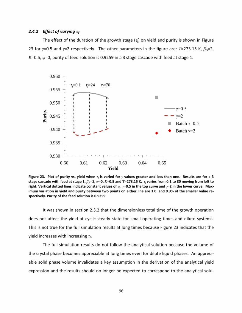
96

2.4.2 Effect of varying τf

The effect of the duration of the growth stage (τf) on yield and purity is shown in Figure

23 for γ=0.5 and γ=2 respectively. The other parameters in the figure are: T=273.15 K, βA=2,

K=0.5, ψ=0, purity of feed solution is 0.9259 in a 3 stage cascade with feed at stage 1.

Figure 23. Plot of purity vs. yield when τf is varied for γ values greater and less than one. Results are for a 3 stage cascade with feed at stage 1, βA=2, ψ=0, K=0.5 and T=273.15 K. τf varies from 0.1 to 80 moving from left to right. Vertical dotted lines indicate constant values of τf. γ=0.5 in the top curve and γ=2 in the lower curve. Max-imum variation in yield and purity between two points on either line are 3.0 and 0.3% of the smaller value re-spectively. Purity of the feed solution is 0.9259.

It was shown in section 2.3.2 that the dimensionless total time of the growth operation

does not affect the yield at cyclic steady state for small operating times and dilute systems.

This is not true for the full simulation results at long times because Figure 23 indicates that the

yield increases with increasing τf.

The full simulation results do not follow the analytical solution because the volume of

the crystal phase becomes appreciable at long times even for dilute liquid phases. An appreci-

able solid phase volume invalidates a key assumption in the derivation of the analytical yield

expression and the results should no longer be expected to correspond to the analytical solu-

0.930

0.935

0.940

0.945

0.950

0.955

0.960

0.60 0.61 0.62 0.63 0.64 0.65

Pu

rity

Yield

γ=0.5

γ=2

Batch γ=0.5

Batch γ=2

τf=0.1 τf=24 τf=70

97

tion. Note that at small times the yield is constant which does correspond to the behavior pre-

dicted by the analytical solution.

The purity also varies slightly as τf is increased but the value of gamma determines

whether the purity increases or decreases. When γ<1 the purity goes through a maximum as τf

is increased. Although this change in purity is small it is important and the dependence of the

maximum purity on different parameters was studied for γ<1. For γ >1 the highest purity is

achieved at very short or very long times and goes through a minimum at intermediate times.

This minimum purity is not of interest and was not studied.

Figure 24 and Figure 25 are plots of the value of τf at which the max purity is reached

and the purity reached at that time vs. a varied operational parameter. The studied parameters

are βA and ψ.

For both βA and ψ the time at which the maximum purity is achieved decreases as the

parameter increases. The behavior of the maximum purity is not the same though as the max-

imum purity decreases as βA increases but increases while ψ increases. No conclusions should

be drawn about the benefits of using high βA or ψ because the effect on yield has not been ad-

dressed. This will be studied in the next section. Figure 24 and Figure 25 do show that the vari-

ation in maximum purity with both βA and ψ is much greater than the variation shown in Figure

23 when τf is varied.

The change in the purity and yield with varying τf is appreciable but is small compared to

the change caused by varying βA or ψ. Subsequent simulation results will be shown for a fixed

operating time during the growth stage in order to simplify analysis given the large number of

parameters. The simulation results indicate that an optimal growth time exists with respect to

purity for any set of parameters with γ<1 and that when γ>1 the shortest possible operating

time will give the highest purity. The yield in either case increases as τf increases. Other factors

such as equipment scheduling, crystal growth blockage of the flow channel, time necessary for

crystal dissolution or downstream processing operations should also be accounted for when

determining the growth time and these may be more important than the slight increases in pur-

ity and yield available at certain values of τf.

98

Figure 24. Growth time at which the maximum purity is achieved and the purity at that time vs. βA. Other simu-lation parameters are ψ=0, γ=0.5, K=0.5 and T=273.15 K for a 3 stage cascade with feed at stage 1. Purity of the feed solution is 0.9259. The solid, gray line is the growth time at which the maximum purity is achieved and corresponds to the left axis. The red dashed line is the maximum purity and corresponds to the right axis.

Figure 25. Growth time at which the maximum purity is achieved and the purity at that time vs. ψ. Other simu-lation parameters are βA=2, γ=0.5, K=0.5 and T=273.15 K for a 3 stage cascade with feed at stage 1. Purity of the feed solution is 0.9259. The solid, gray line is the growth time at which the maximum purity is achieved and corresponds to the left axis. The red dashed line is the maximum purity and corresponds to the right axis.

0.944

0.946

0.948

0.950

0.952

0.954

0.956

0.958

0.960

0.962

0.964

0

10

20

30

40

50

60

70

80

90

100

0 5 10 15 20

Pu

rityτ

f

βA

0.950

0.955

0.960

0.965

0.970

0.975

0

5

10

15

20

25

30

35

40

45

50

0 0.1 0.2 0.3 0.4 0.5

Pu

rityτ

f

ψ

99

2.4.3 Effect of the sweep stream flow rate, feed stage and number of stages

Simulation results showing how the variation of βA and ψ affect the yield and purity of

the semi-continuous counter current crystallization operation are presented in Figure 26.

These results correspond to a 5 stage cascade with the feed at stage 2, a dimensionless resi-

dence time of 3 and a temperature in each stage at the crystallization surface of 273.15 K. The

chemical parameters γ and K are both 0.5 and the purity of the feed solution is 0.9259.

Figure 26. Plot of purity vs. yield when βA is varied for various values of ψ. Results are for a 5 stage cascade with feed at stage 2, τf=3, γ=0.5, K=0.5 and T=273.15 K. Purity of the feed solution is 0.9259. βA varies from a mini-mum equal to the value of ψ for that line to 100 moving left to right in each individual line.

From Figure 26, with increasing βA the yield increases while the purity decreases. Recall

that βA represents the ratio of volumetric incorporation rate constants into the crystal to feed

flow rate. As this value increases, there is more crystal growth compared to flow in the system

so the system behaves more like a batch operation. Higher yields result from larger depletion

of A in the liquid phase. For these values of γ and K, larger depletion of A results in greater in-

corporation of B into the crystal which results in a decrease in purity. The amount of impurity

in the crystal increases as the impurity concentration in the liquid phase increases.

0.90

0.91

0.92

0.93

0.94

0.95

0.96

0.97

0.98

0.99

1.00

0 0.1 0.2 0.3 0.4 0.5 0.6 0.7

Pu

rity

Yield

ψ=0

ψ=0.1

ψ=0.5

ψ=1

Batch

100

The trend with the dimensionless sweep rate (ψ) is in the opposite direction. As the

sweep rate increases, the yield goes down and the purity goes up at a given value of βA. As the

sweep stream increases, there is less crystal in the first tank because more material is swept

further down the cascade. Less crystal means a lower yield but with less depletion of A relative

to B in the liquid phase, the purity of the crystal increases.

The first two curves in Figure 26 for ψ=0 and ψ=0.1 indicate that while the yield de-

creases the purity increases markedly when ψ=0.1. The best possible result in a system with

these values for the chemical-system-specific parameters is higher purity and reduced yield

compared to a batch crystallization. The exact optimal operating condition in terms of ψ and βA

for this system would depend on the relative value of purity to yield but any increase in purity

arising from the use of sweep stream would come at a significant cost in yield. The value of this

trade-off must be evaluated on a case-by-case basis but in general the use of a sweep stream is

not desirable unless higher purity is much more important than maximum yield.

The individual curves for different values of ψ are not the same length. This occurs be-

cause these curves do not represent the same range or values for the parameter βA because

some sets of parameters values do not result in crystalline product being grown. Parameter

sets that lead to zero product were not studied. The smallest value of βA in each line in Figure

26 is equal to the value of ψ for that line.

A very different situation occurs when γ is 2 instead of 0.5. Figure 27 shows the result if

all of the parameters are the same as in Figure 26 except for γ. In this case the purity and yield

of the product both increase as the dimensionless incorporation rate constant of species A in-

creases. It is also apparent that the sweep stream has very little effect on the product purity. A

slight increase in the maximum attainable purity is apparent when a sweep stream is used but

at a significant cost in yield. It is still not possible to achieve a higher yield than a batch crystal-

lization but in this case the purity of the product can exceed the purity of a batch crystallization

at nearly the maximum yield if the dimensionless incorporation rate constant is high enough.

101

Figure 27. Plot of purity vs. yield when βA is varied for various values of ψ. Results are for a 5 stage cascade with feed at stage 2, τf=3, γ=2, K=0.5 and T=273.15 K. Feed solution purity is 0.9259. βA varies from 0.1 to 100 mov-ing left to right in each individual line.

The same behavior at low values of βA is shown in both Figure 26 and Figure 27. High

values of ψ result in purity increasing with increasing βA while small values of ψ result in de-

creasing purity with increasing βA at small values of βA. The behavior at high values of βA is dic-

tated by the system properties K and γ, while at low values of βA the flow nature of the process

is dominant. In the flow dominated regime of Figure 27, there is a transition between the two

types of behavior at a value of ψ between 0.1 and 0.5. Further simulations show that the tran-

sition occurs at approximately ψ=0.35. If this effect is related to the flow nature of the system

then a plot similar to Figure 27 but with much lower growth time should show different beha-

vior. This plot is shown in Figure 28 for the same parameters as in Figure 27 except τf=0.5.

0.90

0.91

0.92

0.93

0.94

0.95

0.96

0.97

0.98

0.99

1.00

0 0.1 0.2 0.3 0.4 0.5 0.6 0.7

Pu

rity

Yield

ψ=0

ψ=0.1

ψ=0.5

ψ=1

Batch

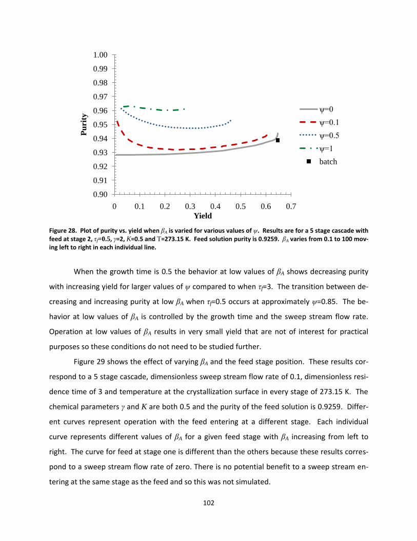
102

Figure 28. Plot of purity vs. yield when βA is varied for various values of ψ. Results are for a 5 stage cascade with feed at stage 2, τf=0.5, γ=2, K=0.5 and T=273.15 K. Feed solution purity is 0.9259. βA varies from 0.1 to 100 mov-ing left to right in each individual line.

When the growth time is 0.5 the behavior at low values of βA shows decreasing purity

with increasing yield for larger values of ψ compared to when τf=3. The transition between de-

creasing and increasing purity at low βA when τf=0.5 occurs at approximately ψ=0.85. The be-

havior at low values of βA is controlled by the growth time and the sweep stream flow rate.

Operation at low values of βA results in very small yield that are not of interest for practical

purposes so these conditions do not need to be studied further.

Figure 29 shows the effect of varying βA and the feed stage position. These results cor-

respond to a 5 stage cascade, dimensionless sweep stream flow rate of 0.1, dimensionless resi-

dence time of 3 and temperature at the crystallization surface in every stage of 273.15 K. The

chemical parameters γ and K are both 0.5 and the purity of the feed solution is 0.9259. Differ-

ent curves represent operation with the feed entering at a different stage. Each individual

curve represents different values of βA for a given feed stage with βA increasing from left to

right. The curve for feed at stage one is different than the others because these results corres-

pond to a sweep stream flow rate of zero. There is no potential benefit to a sweep stream en-

tering at the same stage as the feed and so this was not simulated.

0.90

0.91

0.92

0.93

0.94

0.95

0.96

0.97

0.98

0.99

1.00

0 0.1 0.2 0.3 0.4 0.5 0.6 0.7

Pu

rity

Yield

ψ=0

ψ=0.1

ψ=0.5

ψ=1

batch

103

Figure 29. Plot of purity vs. yield when βA is varied at various feed stages. τf=3, ψ =0.1, γ=0.5, K=0.5, 5 stages, and T=273.15 K. Purity of feed solution is 0.9259. βA varies from 0.1 to 100 moving left to right in each individual line. The curve for feed at stage one has a sweep stream flow rate of zero.

The behavior with changing incorporation rate constant is the same as before; as βA in-

creases, the yield increases and the purity decreases. As the feed stage moves farther down-

stream in the cascade, the yield decreases and the purity increases. Introducing the feed at

stage 2 and using a sweep stream gives lower yield but increased purity compared to feeding at

stage 1 with no sweep stream. A lower sweep stream flow rate would decrease the gap be-

tween the cases for feed at stage 1 and stage 2 but would also diminish the increase in purity

achieved by feeding at tank 2. Again any increase in purity due to the sweep stream is accom-

panied by a decrease in yield.

0.94

0.95

0.96

0.97

0.98

0.99

1.00

0 0.1 0.2 0.3 0.4 0.5 0.6 0.7

Pu

rity

Yield

Feed at Stage 1

Feed at Stage 2

Feed at Stage 3

Feed at Stage 4

Feed at Stage 5

Batch

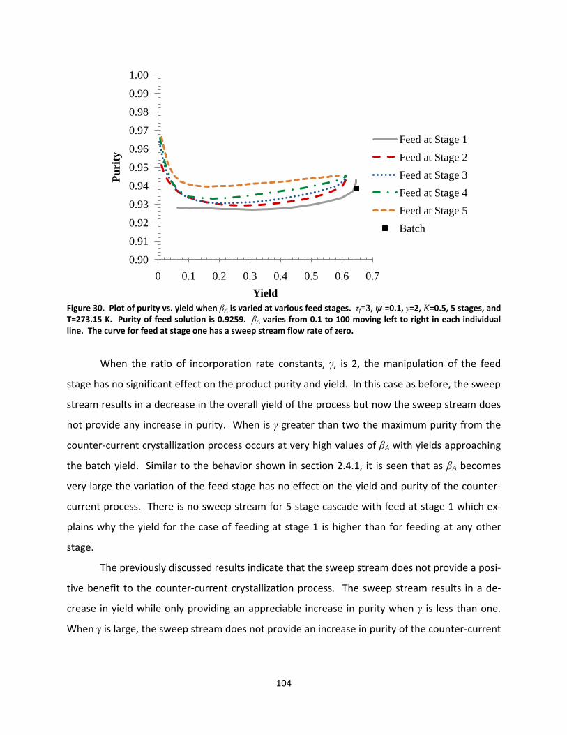
104

Figure 30. Plot of purity vs. yield when βA is varied at various feed stages. τf=3, ψ =0.1, γ=2, K=0.5, 5 stages, and T=273.15 K. Purity of feed solution is 0.9259. βA varies from 0.1 to 100 moving left to right in each individual line. The curve for feed at stage one has a sweep stream flow rate of zero.

When the ratio of incorporation rate constants, γ, is 2, the manipulation of the feed

stage has no significant effect on the product purity and yield. In this case as before, the sweep

stream results in a decrease in the overall yield of the process but now the sweep stream does

not provide any increase in purity. When is γ greater than two the maximum purity from the

counter-current crystallization process occurs at very high values of βA with yields approaching

the batch yield. Similar to the behavior shown in section 2.4.1, it is seen that as βA becomes

very large the variation of the feed stage has no effect on the yield and purity of the counter-

current process. There is no sweep stream for 5 stage cascade with feed at stage 1 which ex-

plains why the yield for the case of feeding at stage 1 is higher than for feeding at any other

stage.

The previously discussed results indicate that the sweep stream does not provide a posi-

tive benefit to the counter-current crystallization process. The sweep stream results in a de-

crease in yield while only providing an appreciable increase in purity when γ is less than one.

When γ is large, the sweep stream does not provide an increase in purity of the counter-current

0.90

0.91

0.92

0.93

0.94

0.95

0.96

0.97

0.98

0.99

1.00

0 0.1 0.2 0.3 0.4 0.5 0.6 0.7

Pu

rity

Yield

Feed at Stage 1

Feed at Stage 2

Feed at Stage 3

Feed at Stage 4

Feed at Stage 5

Batch

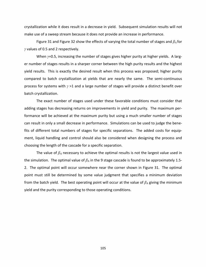
105

crystallization while it does result in a decrease in yield. Subsequent simulation results will not

make use of a sweep stream because it does not provide an increase in performance.

Figure 31 and Figure 32 show the effects of varying the total number of stages and βA for

γ values of 0.5 and 2 respectively.

When γ=0.5, increasing the number of stages gives higher purity at higher yields. A larg-

er number of stages results in a sharper corner between the high purity results and the highest

yield results. This is exactly the desired result when this process was proposed; higher purity

compared to batch crystallization at yields that are nearly the same. The semi-continuous

process for systems with γ >1 and a large number of stages will provide a distinct benefit over

batch crystallization.

The exact number of stages used under these favorable conditions must consider that

adding stages has decreasing returns on improvements in yield and purity. The maximum per-

formance will be achieved at the maximum purity but using a much smaller number of stages

can result in only a small decrease in performance. Simulations can be used to judge the bene-

fits of different total numbers of stages for specific separations. The added costs for equip-

ment, liquid handling and control should also be considered when designing the process and

choosing the length of the cascade for a specific separation.

The value of βA necessary to achieve the optimal results is not the largest value used in

the simulation. The optimal value of βA in the 9 stage cascade is found to be approximately 1.5-

2. The optimal point will occur somewhere near the corner shown in Figure 31. The optimal

point must still be determined by some value judgment that specifies a minimum deviation

from the batch yield. The best operating point will occur at the value of βA giving the minimum

yield and the purity corresponding to those operating conditions.

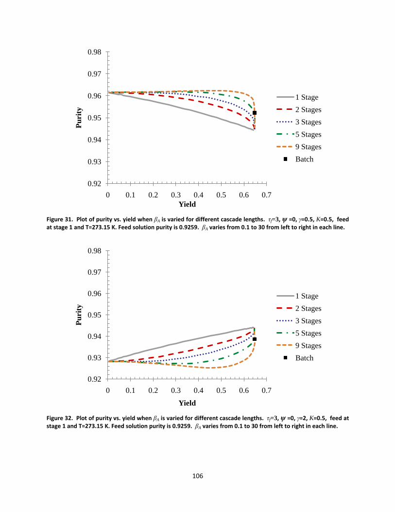
106

Figure 31. Plot of purity vs. yield when βA is varied for different cascade lengths. τf=3, ψ =0, γ=0.5, K=0.5, feed at stage 1 and T=273.15 K. Feed solution purity is 0.9259. βA varies from 0.1 to 30 from left to right in each line.

Figure 32. Plot of purity vs. yield when βA is varied for different cascade lengths. τf=3, ψ =0, γ=2, K=0.5, feed at stage 1 and T=273.15 K. Feed solution purity is 0.9259. βA varies from 0.1 to 30 from left to right in each line.

0.92

0.93

0.94

0.95

0.96

0.97

0.98

0 0.1 0.2 0.3 0.4 0.5 0.6 0.7

Pu

rity

Yield

1 Stage

2 Stages

3 Stages

5 Stages

9 Stages

Batch

0.92

0.93

0.94

0.95

0.96

0.97

0.98

0 0.1 0.2 0.3 0.4 0.5 0.6 0.7

Pu

rity

Yield

1 Stage

2 Stages

3 Stages

5 Stages

9 Stages

Batch

107

For γ=2, the behavior is roughly a mirror image with lower purity being maintained at

higher yields. Figure 32 shows that the proposed crystallization process with the solid output

taken as the product should not be used for systems with γ>1. In this situation the results are

worse than batch crystallization until very high βA at which point the results are the same no

matter the number of stages. A single stage gives the same results as multiple stages and the

extra costs of using multiple stages makes use of a large cascade impractical and unnecessary

when γ>1.

These simulation results indicate that in order to maximize yield the incorporation rate

constant of A must be as large as possible. This can be accomplished by decreasing the flow

rate through the process which results in higher residence times in each tank. The incorpora-

tion could also be increased by increasing the available surface area for crystallization. It will

always be better to have larger surface area for crystallization so systems should be designed

with as much surface area for growth as possible. If this is the case then the flow rate through

the process will be the only method of manipulating the dimensionless incorporation rate con-

stant for an existing set of equipment. While the yield always increases with increasing βA, the

best value of βA must also be chosen with the purity in mind and this will occur at a smaller val-

ue of βA.

Variation of the total number of stages has shown that the counter-current simulation

process can produce better purity than a batch crystallization at comparable when the ratio of

incorporation rate constants is less than one, the surface equilibrium constant is order one or

less and βA is chosen carefully. This is the stated goal of the proposed process and the condi-

tions under which it is attainable have been made clearer. For systems with γ>1 the variation of

the cascade length shows that a multi-stage process has no benefit over a single stage. It was

seen in section 2.4.1 that higher values of γ result in lower purities except at very high values of

βA but in this section it was seen that this is the case at any number of stages and the proposed

process has no benefit when γ>1. The semi-continuous process will be advantageous for sys-

tems with γ<1 and K<O(1) in cascades with the largest possible number of stages and no sweep

stream.

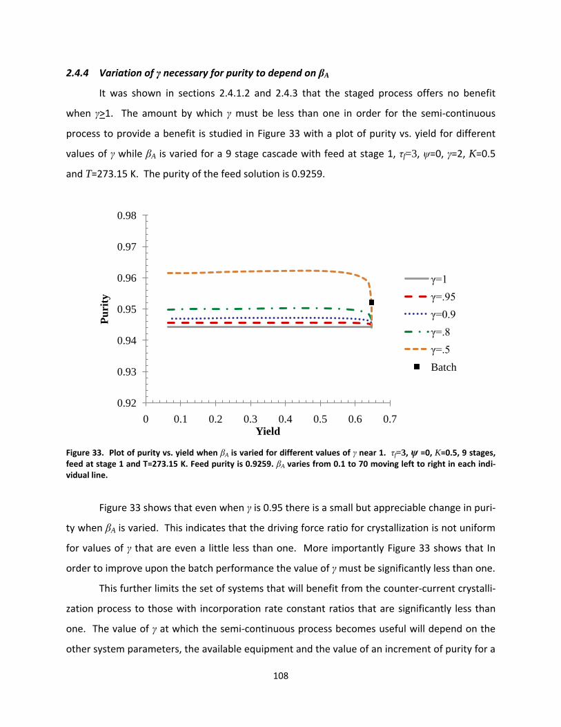
108

2.4.4 Variation of γ necessary for purity to depend on βA

It was shown in sections 2.4.1.2 and 2.4.3 that the staged process offers no benefit

when γ>1. The amount by which γ must be less than one in order for the semi-continuous

process to provide a benefit is studied in Figure 33 with a plot of purity vs. yield for different

values of γ while βA is varied for a 9 stage cascade with feed at stage 1, τf=3, ψ=0, γ=2, K=0.5

and T=273.15 K. The purity of the feed solution is 0.9259.

Figure 33. Plot of purity vs. yield when βA is varied for different values of γ near 1. τf=3, ψ =0, K=0.5, 9 stages, feed at stage 1 and T=273.15 K. Feed purity is 0.9259. βA varies from 0.1 to 70 moving left to right in each indi-vidual line.

Figure 33 shows that even when γ is 0.95 there is a small but appreciable change in puri-

ty when βA is varied. This indicates that the driving force ratio for crystallization is not uniform

for values of γ that are even a little less than one. More importantly Figure 33 shows that In

order to improve upon the batch performance the value of γ must be significantly less than one.

This further limits the set of systems that will benefit from the counter-current crystalli-

zation process to those with incorporation rate constant ratios that are significantly less than

one. The value of γ at which the semi-continuous process becomes useful will depend on the

other system parameters, the available equipment and the value of an increment of purity for a

0.92

0.93

0.94

0.95

0.96

0.97

0.98

0 0.1 0.2 0.3 0.4 0.5 0.6 0.7

Pu

rity

Yield

γ=1

γ=.95

γ=0.9

γ=.8

γ=.5

Batch

109

specific chemical system. Numerical simulations can be used to determine the necessary value

if the other chemical parameters are known. In general, the lowest possible value of γ will re-

sult in the best performance in comparison to batch crystallization as long as that value is below

a threshold value determined by all of the chemical system parameters

2.4.5 Consideration of possible combinations of K and γ

The previous figures have shown that the crystallization process as described in section

2.1 is useful only when K is less than order one and γ is less than one. But it is useful to consid-

er alternative methods of employing the proposed process in order to achieve productive re-

sults from a wider array of chemical systems. The possible combinations of K and γ can be bro-

ken down as K and γ greater than 1; K and γ less than one; K greater than one and γ less than

one; and K less than one and γ greater than one. The previous results have shown that when K

and γ are both less than one the crystallization process as described above produces the desired

outcome as long as γ is a system specific amount less than unity.

The process proposed in section 2.1 has two outputs; the crystal that is taken as the

product and the liquid effluent from the growth operation. For systems where K and γ are not

both less than one, analysis of the effluent stream concentration is informative. The following

plots will show the purity vs. yield for both the crystal product and the liquid effluent stream for

different values of the chemical system specific parameters

The reported values of yield and purity of the effluent stream are an average over the

entire growth cycle. The yield of the effluent stream (yL) is determined by integrating the

product of the flow rate out of the final tank and the concentration of component A in the final

tank and then dividing this integral by the total amount of component A put into the system.

0

f

N AN

L

f

dy

(2.96)

where the subscript N denotes a property of the last tank in the cascade.

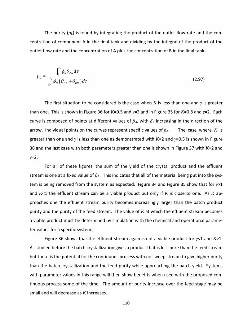
110

The purity (pL) is found by integrating the product of the outlet flow rate and the con-

centration of component A in the final tank and dividing by the integral of the product of the

outlet flow rate and the concentration of A plus the concentration of B in the final tank.

0

0

f

f

N AN

L

N AN BN

dp

d

(2.97)

The first situation to be considered is the case when K is less than one and γ is greater

than one. This is shown in Figure 36 for K=0.5 and γ=2 and in Figure 35 for K=0.8 and γ=2. Each

curve is composed of points at different values of βA, with βA increasing in the direction of the

arrow. Individual points on the curves represent specific values of βA. The case where K is

greater than one and γ is less than one as demonstrated with K=2 and γ=0.5 is shown in Figure

36 and the last case with both parameters greater than one is shown in Figure 37 with K=2 and

γ=2.

For all of these figures, the sum of the yield of the crystal product and the effluent

stream is one at a fixed value of βA. This indicates that all of the material being put into the sys-

tem is being removed from the system as expected. Figure 34 and Figure 35 show that for γ>1

and K<1 the effluent stream can be a viable product but only if K is close to one. As K ap-

proaches one the effluent stream purity becomes increasingly larger than the batch product

purity and the purity of the feed stream. The value of K at which the effluent stream becomes

a viable product must be determined by simulation with the chemical and operational parame-

ter values for a specific system.

Figure 36 shows that the effluent stream again is not a viable product for γ<1 and K>1.

As studied before the batch crystallization gives a product that is less pure than the feed stream

but there is the potential for the continuous process with no sweep stream to give higher purity

than the batch crystallization and the feed purity while approaching the batch yield. Systems

with parameter values in this range will then show benefits when used with the proposed con-

tinuous process some of the time. The amount of purity increase over the feed stage may be

small and will decrease as K increases.

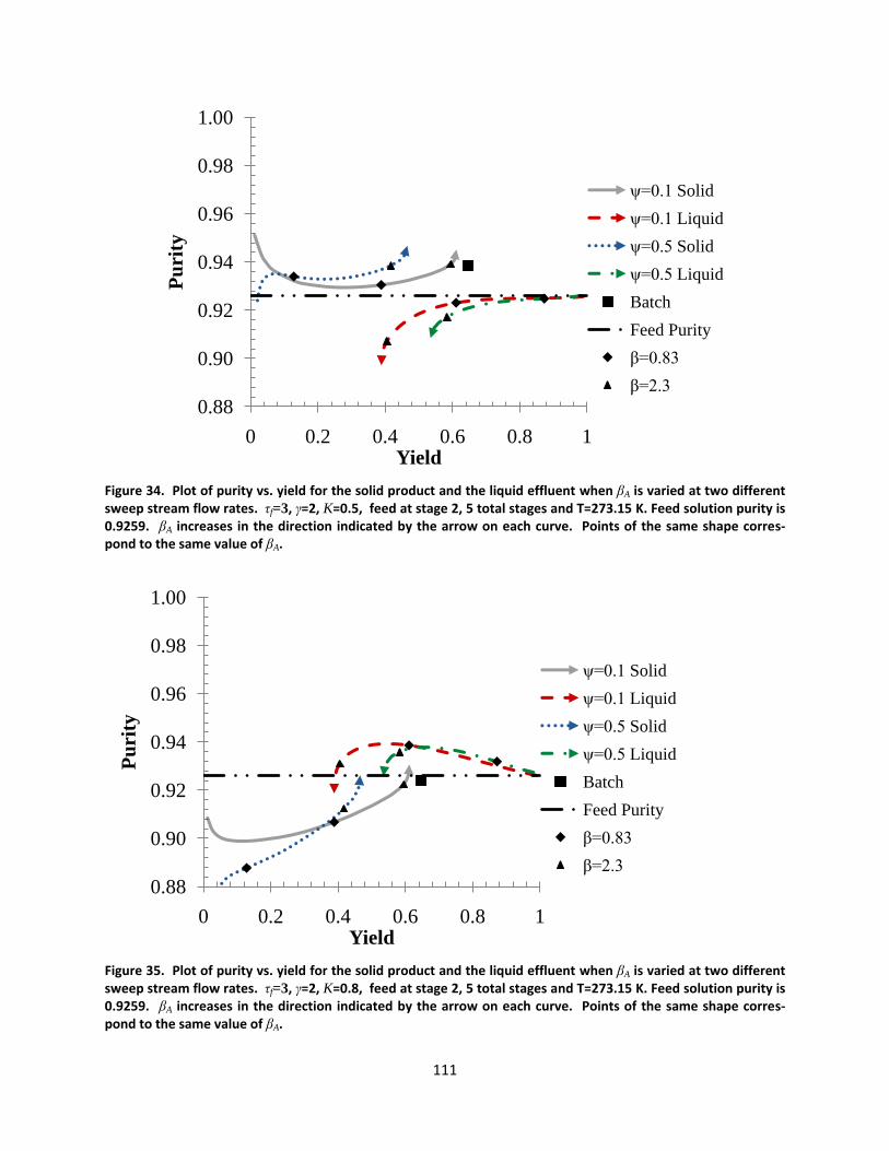
111

Figure 34. Plot of purity vs. yield for the solid product and the liquid effluent when βA is varied at two different sweep stream flow rates. τf=3, γ=2, K=0.5, feed at stage 2, 5 total stages and T=273.15 K. Feed solution purity is 0.9259. βA increases in the direction indicated by the arrow on each curve. Points of the same shape corres-pond to the same value of βA.

Figure 35. Plot of purity vs. yield for the solid product and the liquid effluent when βA is varied at two different sweep stream flow rates. τf=3, γ=2, K=0.8, feed at stage 2, 5 total stages and T=273.15 K. Feed solution purity is 0.9259. βA increases in the direction indicated by the arrow on each curve. Points of the same shape corres-pond to the same value of βA.

0.88

0.90

0.92

0.94

0.96

0.98

1.00

0 0.2 0.4 0.6 0.8 1

Pu

rity

Yield

ψ=0.1 Solid

ψ=0.1 Liquid

ψ=0.5 Solid

ψ=0.5 Liquid

Batch

Feed Purity

β=0.83

β=2.3

0.88

0.90

0.92

0.94

0.96

0.98

1.00

0 0.2 0.4 0.6 0.8 1

Pu

rity

Yield

ψ=0.1 Solid

ψ=0.1 Liquid

ψ=0.5 Solid

ψ=0.5 Liquid

Batch

Feed Purity

β=0.83

β=2.3

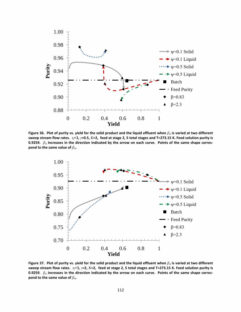
112

Figure 36. Plot of purity vs. yield for the solid product and the liquid effluent when βA is varied at two different sweep stream flow rates. τf=3, γ=0.5, K=2, feed at stage 2, 5 total stages and T=273.15 K. Feed solution purity is 0.9259. βA increases in the direction indicated by the arrow on each curve. Points of the same shape corres-pond to the same value of βA.

Figure 37. Plot of purity vs. yield for the solid product and the liquid effluent when βA is varied at two different sweep stream flow rates. τf=3, γ=2, K=2, feed at stage 2, 5 total stages and T=273.15 K. Feed solution purity is 0.9259. βA increases in the direction indicated by the arrow on each curve. Points of the same shape corres-pond to the same value of βA.

0.88

0.90

0.92

0.94

0.96

0.98

1.00

0 0.2 0.4 0.6 0.8 1

Pu

rity

Yield

ψ=0.1 Solid

ψ=0.1 Liquid

ψ=0.5 Solid

ψ=0.5 Liquid

Batch

Feed Purity

β=0.83

β=2.3

0.70

0.75

0.80

0.85

0.90

0.95

1.00

0 0.2 0.4 0.6 0.8 1

Pu

rity

Yield

ψ=0.1 Solid

ψ=0.1 Liquid

ψ=0.5 Solid

ψ=0.5 Liquid

Batch

Feed Purity

β=0.83

β=2.3

113

When both γ and K are greater than one, as in Figure 37, the effluent stream has higher

purity and higher yield than the batch result. This is an ideal result as the yield is seen to be

significantly greater than the batch yield while still allowing increased purity. The proposed

crystallization process is beneficial for systems with γ and K greater than one except that the

stream previously called the “waste” stream should now be taken as the product. The crystal

product is now waste and can be discarded.

This situation is ideal because the product is a liquid with high yield and purity in com-

parison to batch crystallization but is not expected to be common. K greater than one indicates

that the impurity has a higher concentration in the crystal than the component of interest and

γ>1 indicates that the impurity is incorporated into the crystal faster than the component of

interest. These two properties may tend to happen together but it is expected that in general

the component of interest will favor incorporation of itself in both rate and amount. Systems

with γ>1 and K>1 are expected to be very rare but will provide excellent results with the pro-

posed process if the liquid effluent is taken as the product.

A summary of the benefits of the proposed process for different combinations of the

chemical system specific parameters is given in Figure 38. The actual parameter values for real

systems are expected to most often fall in the lower-left quadrant but these parameters must

be determined experimentally.

114

Figure 38. Diagram of different combinations of the chemical system specific parameter and their utility with the proposed counter-current crystallization process.

2.4.6 Comparison of Operation with and without a Liquid Handling Tank

To this point the simulation has been used to study the system when the liquid contents

of the final tank are retained between growth cycles. The results from a process where this liq-

uid is discarded will now be compared to the previous results.

First the purity vs. yield of the solid product will be shown for a range of βA values at dif-

ferent values of γ for the process with and without the liquid handling tank. These results are

for a system with the same number of active tanks such that the overall process when a liquid

handling tank is used has one additional tank. These results are shown in Figure 39.

γ > 1

γ < 1

K > 1 K < 1

SOMETIMES

use with counter-current

process with liquid

effluent taken as product.

DO


process with liquid

effluent taken as product.

DO


process with solid taken

as product.

SOMETIMES


process with solid taken

as product.

115

Figure 39. Plot of purity vs. yield comparing process with retention of liquid from final stage with removal of liquid from final stage when βA is varied at various values of the constant ratio γ. τf=2, ψ=0, 3 stages, feed at stage 1, K=0.5, and T=273.15 K. βA varies from 0.1 to 30 moving left to right in each individual line. Individual points correspond to the batch comparison points for different values of γ. The purity of the feed solution is 0.9259.

Figure 39 indicates that there is a very small difference in the performance of the

process with and without the liquid handling tank. These results indicate that the decision to

keep or discard the liquid contents of the last tank depend on the value of γ. At γ=0.9 better

results are achieved when keeping the liquid while at γ=0.5 discarding the liquid gives better

results. The difference though in all cases is slight and a different comparison is necessary to

decide which approach is better in general.

The comparison so far has been between systems with the same number of active tanks

but a more appropriate comparison could be processes with the same number of total tanks.

So that a cascade with three active tanks and a liquid handling tank where the liquid from the

last tank is retained should be compared to a process with four active tanks where the liquid

from the last tank is discarded. The results for this comparison are given in Figure 40 as a plot

of yield vs. purity at different values of βA.

0.94

0.95

0.96

0.97

0.98

0.99

1.00

0 0.1 0.2 0.3 0.4 0.5 0.6 0.7

Pu

rity

Yield

Keep, γ=0.1

Discard, γ=0.1

Keep, γ=0.5

Discard, γ=0.5

Keep, γ=0.9

Discard, γ=0.9

Batch, γ=0.1

Batch, γ=0.5

Batch, γ=0.9

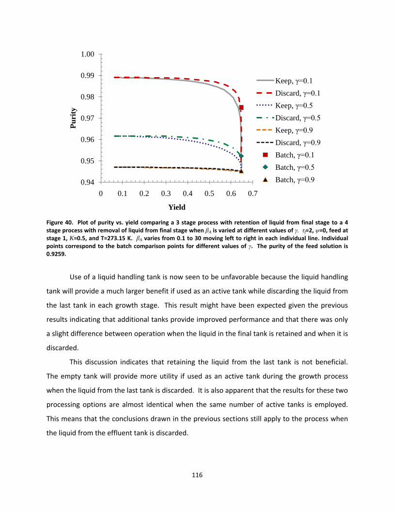
116

Figure 40. Plot of purity vs. yield comparing a 3 stage process with retention of liquid from final stage to a 4 stage process with removal of liquid from final stage when βA is varied at different values of γ. τf=2, ψ=0, feed at stage 1, K=0.5, and T=273.15 K. βA varies from 0.1 to 30 moving left to right in each individual line. Individual points correspond to the batch comparison points for different values of γ. The purity of the feed solution is 0.9259.

Use of a liquid handling tank is now seen to be unfavorable because the liquid handling

tank will provide a much larger benefit if used as an active tank while discarding the liquid from

the last tank in each growth stage. This result might have been expected given the previous

results indicating that additional tanks provide improved performance and that there was only

a slight difference between operation when the liquid in the final tank is retained and when it is

discarded.

This discussion indicates that retaining the liquid from the last tank is not beneficial.

The empty tank will provide more utility if used as an active tank during the growth process

when the liquid from the last tank is discarded. It is also apparent that the results for these two

processing options are almost identical when the same number of active tanks is employed.

This means that the conclusions drawn in the previous sections still apply to the process when

the liquid from the effluent tank is discarded.

0.94

0.95

0.96

0.97

0.98

0.99

1.00

0 0.1 0.2 0.3 0.4 0.5 0.6 0.7

Pu

rity

Yield

Keep, γ=0.1

Discard, γ=0.1

Keep, γ=0.5

Discard, γ=0.5

Keep, γ=0.9

Discard, γ=0.9

Batch, γ=0.1

Batch, γ=0.5

Batch, γ=0.9

117

2.5 Summary of Process Description and Simulation

A counter-current crystallization process has been proposed that operates in a semi-

continuous manner and seeks to eliminate multi-phase flows. This is done by confining crystal

growth to fixed growth surfaces and performing a liquid transfer operation along with syste-

matic shifting of the feed and outlet points along a cascade of tanks. The two outputs from this

process are a solid crystalline product and a liquid effluent stream. This process is complicated

but has operational similarities to simulated moving bed chromatography. The benefits of the

proposed process are multiple recrystallizations to allow for improved purity and the elimina-

tion of multi-phase flow handling.

The yield of a crystallization process is determined by the concentration and flow rate of

the effluent stream. The concentration of the effluent is constrained by the solubility of species

A in the solvent of interest. A batch crystallization run until completion will provide the maxi-

mum possible yield and any continuous crystallization process will at best be able to match this

batch yield unless the effluent stream is altered.

A model has been developed for batch crystallization and the proposed semi-

continuous, counter-current crystallization operation. The system specific parameters CA*(T),

K, γ and n must be measured experimentally before using this simulation to predict the separa-

tion performance in the proposed counter-current crystallization operation. This simulation

indicates that this process can give superior purity and comparable yield to batch crystallization

run until completion from both the crystalline product and the liquid effluent for different val-

ues of the parameters K and γ.

The solid crystalline output is the appropriate product to use when the ratio of the in-

corporation rate constants of the impurity to the incorporation rate constant of the product (γ)

is less than one and K is order one or less. The liquid effluent should be taken as the product

when γ>1 and K is very close to or greater than one. This liquid effluent is the waste stream as

described in the original description of the process but for certain parameter values the simula-

tion results indicate that it will provide a liquid product with higher purity and yield than batch

crystallization. In this scenario the crystallized solid should be discarded as waste.

118

Simulation results also indicate that the use of a sweep stream and tanks upstream of

the feed point should not be employed when the solid is taken as the product because of the

negative effect on yield. The sweep stream was seen to give increased purity but only at a sig-

nificant cost in product yield. A large number of stages was found to provide higher purity at

yields approaching the batch yield when γ<1. The benefit of increasing the number of stages

decreases as more stages are added so this must be weighed against capital and operational

costs of larger cascades.

Use of the process with the liquid contents from the effluent tank discarded after each

growth cycle was found to be better than operation with retention of the liquid in the effluent

tank by use of an extra liquid handling tank. The difference in performance for these two oper-

ating principles was found to be very small when an equal number of active tanks were com-

pared but use of the liquid handling tank as an active tank for crystallization provides superior

results. This is in agreement with the conclusion that more tanks provide better performance.

Results generated from simulations making use of the liquid handling tank are also appropriate

for the system without a liquid handling tank if the number of active stages is held constant..

Key assumptions involved in developing this model are the equilibrium expression at the

liquid-solid interface and the expressions for crystal growth. The equilibrium constant K is as-

sumed to be only a function of temperature. Experimental work must be done to validate the

assumptions in this model and provide input to help refine this model to better predict real be-

havior. Batch experiments used to test the validity of this model are discussed in Chapters 3

and 4.

119

3. Preliminary Batch Experiments

Initial investigations of the impurity distribution between the liquid and solid phases

during batch crystallization were performed before development of the model described in

Chapter 2. This work was done at the St. Johann campus of Novartis International AG in Basel,

Switzerland, to take advantage of existing experimental setups for performing traditional

seeded, batch crystallizations.

The goal of these experiments was to measure how different parameters affect the dis-

tribution of impurity between solid and liquid phases. The effect of the final temperature, ini-

tial concentration of the component of interest and the initial purity of the solution were stu-

died. The chemical compounds used in these experiments will be described first followed by an

outline of the experimental method and finally the results from the batch experiments.

3.1 Chemical System for Experimentation

Cyclosporine A is a member of a family of similar structures that was used as the chemi-

cal system for these batch experiments. Cyclosporine A is a large ring shaped compound com-

posed of 11 amino acids. The structure of cyclosporine is shown in Figure 41. The cyclospo-

rines are a good choice for batch experimentation because they have a strongly temperature

dependent solubility and consequently readily crystallize from solution.

Cyclosporine A is the desired compound but the raw material contains at least 11 dis-

cernible impurities which are relatives of cyclosporine A. These impurities have a range of very

small structural differences including the presence of an extra double bond, an ethyl instead of

a methyl group or a single chemical bond connecting two adjacent amino acids in a slightly dif-

ferent way. These very slight structural differences make it likely that cyclosporine A forms sol-

id solutions with at least some of the other cyclosporines. It is very difficult to obtain extremely

pure samples of different cyclosporines due to their similar structures and so phase behavior

for pairs of cyclosporines has not been measured and solid solution behavior has not been

proven in the literature.

120

Figure 41. Chemical Structure of Cyclosporine A.

The raw material for these experiments as supplied by Novartis consisted of 89% by

mass cyclosporine A and 11% total impurities. Of those 11% impurities, 9-10% are other cyc-

losporine molecules and the remaining 1-2% are solvents or other trace materials.

3.2 Experimental Method

The experiments were conducted in a stirred batch vessel under temperature control.

Experimental data consisted of the temperature profile and HPLC analysis of the starting ma-

terial, product, mother liquor and wash liquor. Additionally, UV-Vis measurements were col-

lected for some experiments. The UV-Vis measurements were obtained from a probe placed in

the reaction vessel which provided real-time absorption information.

All experiments were carried out using the following approach. The starting solution

was heated to 500 C in order to dissolve all of the solids. The solution was then cooled at a rate

of 0.5 K/min to the temperature at which the solution was 2.5 times supersaturated as deter-

121

mined from the solubility curve for cyclosporine A. The solution was then seeded and the tem-

perature was held constant for 1 hour. The solution was then cooled or heated to the final

temperature at a rate of 0.3-0.5 K/min after which it was held at this temperature for 0-15

hours.

Experiments were conducted in a FlexyLab controlled lab reactor. A 100 mL reactor

vessel equipped with mechanical stirrer and temperature probe were used. Temperature con-

trol was achieved through cooling or heating of the external wall of the reactor. The crystals

grown during an experiment were vacuum filtered and washed with a small amount of acetone

before being dried in an oven overnight.

The mother liquor and wash liquid were collected separately in order to determine if the

wash liquid was resulting in significant dissolution of the crystals. If the wash liquid concentra-

tion is very similar to the mother liquor concentration then the wash is likely succeeding in re-

moving some of the mother liquor stuck to crystals as opposed to dissolving some of the crys-

talline product.

The concentrations from the starting material, crystalline product, mother liquor and

wash liquid were calculated from HPLC data in the following manner. The liquid phases were

used directly while a little of the solid product was dissolved in acetone for HPLC analysis. A

calibration chart for cyclosporine A was provided by Novartis and it was used to calculate the

concentration of all the cyclosporines in a HPLC sample. The use of the cyclosporine A calibra-

tion chart for all cyclosporines assumes that absorbtivity for all cyclosporines is the same. Giv-

en the large size and similar structure of the molecules, this was deemed a good assumption.

The amounts for each species in the feed, product, mother liquor and wash liquor were

entered into a mass balance. Good results were achieved in general with the overall mass bal-

ances closing to within 10% in most cases, and often closer to 5%. Individual data points for

different impurities were neglected in separation analysis if the mass balance was off by more

than 15%.

The variables of interest in this study were the final temperature, the initial concentra-

tion and the initial purity. The final temperatures used were 2.5, 20, 30 and 350C. The initial

concentrations were 0.18, 0.264 and 0.131 mass of cyclosporine A per unit mass total solution.

122

The initial purities used were 0.79, 0.89 and 0.94 mass of cyclosporine A per unit mass solids.

Other possible variables include the cooling rate and the holding time. In order to minimize ex-

periments and to focus on the most important factors, the cooling rate and the holding time

were chosen so that they had as little effect as possible on the result. Experiments were done

to show that holding times greater than or equal to 4 hours have no effect on the product com-

position and that cooling rates less than 0.7 K/min after seeding also did not affect the results.

3.3 Experimental Results

The representation of the depletion behavior that was determined to be most useful is

the separation factor. It is defined by the following equation.

,

,

,

,

j S

j L

AjA S

A L

C

C

CC

(3.1)

where C is a concentration, subscript A refers to cyclosporine A (or more generally the compo-

nent of interest), subscript j refers to a specific impurity, L refers to the liquid phase and S re-

fers to the crystal phase. This quantity represents the ratio of the distributions of an impurity

and the component of interest between the crystal and the liquid phases. A separation factor

of 1 indicates that no purification has taken place; the crystal product has the same purity as

the initial solution. A separation factor of 0 indicates that there is none of that impurity in the

crystal which means that a perfect separation has occurred. A separation factor that is greater

than one indicates that the impurity has been concentrated in the crystal compared to the tar-

get component.

The separation factor measured in these experiments is not an equilibrium property.

The time dependent concentration profiles of the solid and liquid phases during crystallization

affect the measured value. If the crystallization were to be operated at a constant temperature

with very small crystal particles until equilibrium is reached in both the solid and liquid phases,

123

then the measured separation factor will be equal to the surface equilibrium constant at the

temperature of the crystallization as defined in the model presented in Chapter 2. This would

be a difficult condition to approach experimentally because enough time must be allowed for

diffusion to occur in the solid phase so that any concentration profiles are smoothed out.

3.3.1 Cyclosporine C, U and V

The measured separation factors and yield as functions of final temperature, initial con-

centration and initial purity for three cyclosporine impurities are shown in Figure 42 through

Figure 48. The points in each graph correspond to the situation where all parameters are held

constant except for the one varied along the x-axis. For example, in a plot where temperature

is varied the initial concentration and purity are held constant for each experiment.

Figure 42. Experimental separation factors as a function of final temperature from batch experiments for three cyclosporine impurities.

0.00

0.05

0.10

0.15

0.20

0.25

0.30

0.35

0.40

0 10 20 30 40

α

Final Temperature (0C)

Cyclosporine C

Cyclosporine U

Cyclosporine V

124

Figure 43. Yield as a function of final temperature from batch experiments.

Figure 42 shows that there is generally a clear trend with the final temperature showing

that the separation factor increases with increasing temperature. Increasing values of the se-

paration factor indicate worse separations so increasing temperature results in less separation

of the impurity from cyclosporine A.

It is also seen in Figure 43 that yield decreases with increasing final temperature. As

temperature increases the solubility of cyclosporine A in the solvent increases and so yield must

decrease while at higher temperatures it is more likely for the impurity molecules to be in-

cluded in the crystal and so it is expected that the separation will be worse. This is the behavior

shown in these plots. The relationship between the separation factor and temperature is seen

to be generally linear.

0%

10%

20%

30%

40%

50%

60%

70%

80%

90%

100%

0 10 20 30 40

Yie

ld


125

Figure 44. Separation factor as a function of initial concentration for three cyclosporine impurities from batch experiments.

Figure 45. Yield as a function of initial cyclosporine A concentration from batch experiments.

0.00

0.05

0.10

0.15

0.20

0.25

0 0.1 0.2 0.3 0.4

α

Initial Mass Fraction of Cyclosporine A

Cyclosporine C

Cyclosporine U

Cyclosporine V

0%

10%

20%

30%

40%

50%

60%

70%

80%

90%

100%

0 0.1 0.2 0.3 0.4

Yie

ld

Initial Mass Fraction of Cyclosporine A

126

Figure 44 shows that there is no apparent trend of the separation factor with the initial

concentration. The yield is seen in Figure 45 to increase as the initial concentration increases.

At a given temperature, increasing the starting concentration means the initial supersaturation

is increased while the saturation concentration is unchanged. A larger driving force allows

more crystal to be generated under experimental conditions where steady state is approached.

Steady state is approached under the conditions of these experiments.

Figure 46 shows that the separation factor decreases slightly with increasing initial puri-

ty. This indicates that purer starting materials lead to purer products. This result indicates that

multiple recrystallizations would result in better purity when separating cyclosporine A from its

impurities. The yield is seen in Figure 47 to not depend on the initial purity. The fact that the

yield does not change is good because it supports the assumption that the solubility behavior

can be determined by ignoring all of the impurities in solution. When approaching equilibrium,

the yield is determined by the initial supersaturation. If the initial concentration of cyclosporine

A is unchanged then the supersaturation is unchanged and the same yield will be achieved if

the amount of impurities does not affect the solubility of cyclosporine A in the solvent.

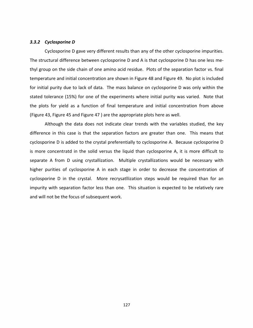
127

3.3.2 Cyclosporine D

Cyclosporine D gave very different results than any of the other cyclosporine impurities.

The structural difference between cyclosporine D and A is that cyclosporine D has one less me-

thyl group on the side chain of one amino acid residue. Plots of the separation factor vs. final

temperature and initial concentration are shown in Figure 48 and Figure 49. No plot is included

for initial purity due to lack of data. The mass balance on cyclosporine D was only within the

stated tolerance (15%) for one of the experiments where initial purity was varied. Note that

the plots for yield as a function of final temperature and initial concentration from above

(Figure 43, Figure 45 and Figure 47 ) are the appropriate plots here as well.

Although the data does not indicate clear trends with the variables studied, the key

difference in this case is that the separation factors are greater than one. This means that

cyclosporine D is added to the crystal preferentially to cyclosporine A. Because cyclosporine D

is more concentratd in the solid versus the liquid than cyclosporine A, it is more difficult to

separate A from D using crystallization. Multiple crystallizations would be necessary with

higher purities of cyclosporine A in each stage in order to decrease the concentration of

cyclosporine D in the crystal. More recrysatllization steps would be required than for an

impurity with separation factor less than one. This situation is expected to be relatively rare

and will not be the focus of subsequent work.

128

Figure 46. Separation factor as a function of initial purity of cyclosporine A for three cyclosporine impurities from batch experiments. Purity is defined as mass fraction of cyclosporine A on a solvent free basis.

Figure 47. Yield as a function of initial purity from batch experiments. Purity is defined as mass fraction of cyc-losporine A on a solvent free basis.

0.00

0.05

0.10

0.15

0.20

0.25

0.30

0.35

0.40

0.75 0.8 0.85 0.9 0.95

Sep

ara

tion

Fact

or

Initial Purity Cyclosporine A

Cyclosporine C

Cyclosporine U

Cyclosporine V

0%

10%

20%

30%

40%

50%

60%

70%

80%

90%

100%

0.75 0.8 0.85 0.9 0.95

Yie

ld

Initial Purity Cyclosporine A

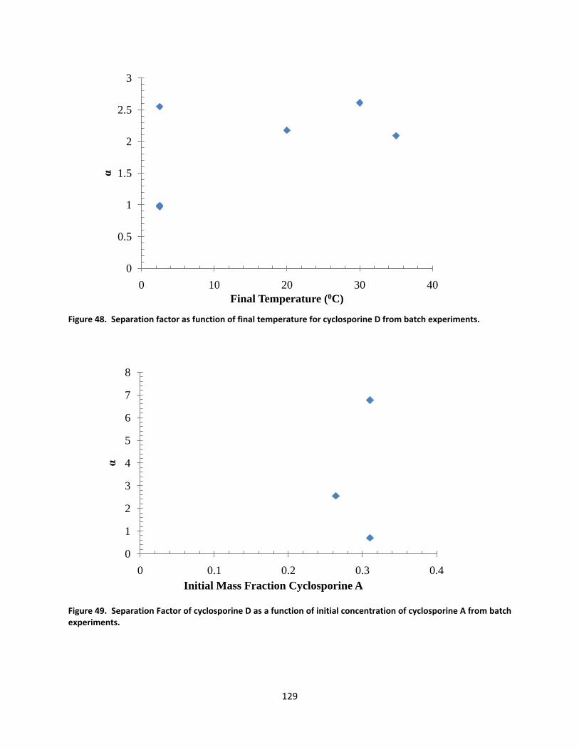
129

Figure 48. Separation factor as function of final temperature for cyclosporine D from batch experiments.

Figure 49. Separation Factor of cyclosporine D as a function of initial concentration of cyclosporine A from batch experiments.

0

0.5

1

1.5

2

2.5

3

0 10 20 30 40

α


0

1

2

3

4

5

6

7

8

0 0.1 0.2 0.3 0.4

α

Initial Mass Fraction Cyclosporine A

130

3.4 Summary and Conclusions

Experimental studies of seeded batch crystallization operations have been performed in

order to gain understanding of the impurity distribution in the crystal product. The separation

factor given by the ratio of impurity and component of interest partitioning between the crystal

and liquid phase was used to quantify this impurity distribution. Separation factors were calcu-

lated from experimental measurements where the final temperature, initial concentration of

cyclosporine A and initial purity of cyclosporine A were varied.

Most of the separation factors were found to be less than one indicating the crystal is

more pure than the starting material in terms of that impurity. Cyclosporine D was conversely

found to have a separation factor greater than one indicating that the crystal is less pure with

respect to D than the starting material. Impurities with separation factors greater than one will

require more re-crystallizations to achieve high purity.

The majority of impurities had separation factors that were found to be linearly depen-

dence on final temperature, independent of initial concentration and slightly dependent on ini-

tial purity. These results suggest that for modeling purposes the separation factor should be

treated solely as a function of temperature.

The yield was unaffected by the purity of the starting material which means the satura-

tion data as a function of temperature for the component of interest can be used in the pres-

ence of impurities when the impurities are similar and they are present in small quantity. This

is an assumption used in the model development in Chapter 2 and is found to be valid here for

cyclosporine A and its impurities.

The conclusions drawn from these experiments must be treated carefully when applied

to the process described and modeled in Chapter 2. These experiments were performed on

batch systems with a large distribution of crystal particle sizes. For processes where crystalliza-

tion is confined to a surface there could be significantly different behavior.

The batch experiments in this chapter also used a series of temperature gradients that

will affect the generated crystals. Chapter 4 will discuss experiments performed that are more

directly applicable to the semi-continuous counter-current crystallization operation proposed in

Chapter 2.

131

4. Model Validation by Batch Crystallization

The process defined in the chapter 2 required a number of assumptions and those as-

sumptions must be tested against experimental data. Experimental data are also required to

determine the necessary model parameters for a particular chemical system. Setting up the full

semi-continuous process would require a large amount of equipment and time so batch expe-

riments are used instead because they are simpler to setup and perform and can provide the

necessary information for model validation and parameter estimation.

The model developed for batch crystallization in Chapter 2 can be used for experimental

model validation. This chapter will detail further analysis of the batch model to gain insight into

the expected behavior during experimentation and discuss the experimental setup and results.

4.1 Further Analysis of Batch Model

The liquid phase concentration expressions developed in section 2.2.2 can be extended

further to give information about the overall distribution of impurity between liquid and solid

phases and the concentration profile in the solid phase. The dimensionless concentration pro-

files for A and B during batch crystallization are given again in equations (4.1) and (4.2). Recall

that these expressions were derived assuming the liquid volume is constant (dilute system), the

temperature is constant and the parameter n is equal to one.

2* *

2 1A A A e (4.1)

2

*

*

11 1

11 1

A

B

A

Ke

K

(4.2)

An overall separation factor and the mole fraction of impurity in the solid were derived.

The overall separation factor is defined in equation (4.3). This factor is also discussed in section

1.2.2.

132

BcA

B Ac

(4.3)

The difference between the separation factor and the surface equilibrium expression used in

the model is that the separation factor is defined with the average concentration of the phases

instead of surface solid and equilibrium liquid concentrations. Also, the separation factor is not

an equilibrium quantity because its value depends on the history of the solution which defines

the growth of crystal and incorporation of impurity. The surface equilibrium expression estab-

lishes a temperature dependent relationship between the equilibrium liquid phase concentra-

tions and the surface solid phase concentrations no matter what the concentration profiles of

the two phases have looked like up to that point.

The separation factor can be expressed as follows by recalling that the total mass of

each component is constant and that the liquid volume is assumed constant.

*

*

* *

11

111 1 11

1

1 111 1

1

A

ABcA A B B

B Ac b A

A A A

Ke

eK

e

(4.4)

The other quantity derived from this model is the surface mole fraction of impurity in

the crystal (xBcS). This variable as a function of time or total crystal mass gives the concentra-

tion gradient in the crystal. First combine equations (2.32), (2.33), (2.34) and (2.36) to give eq-

uation (4.5).

* **

*

* *

s A A AA AAc

s

bc BA B

B

A A A

K

K

(4.5)

133

The mole fraction of the impurity in the solid at the surface is then given by equation

(4.6).

0 0

0 0

1 1

1 1

ss BcBc s ss s

Ac AcA BBc Ac

s s

A B Bc Bc

Cx

C C CC C

C C C

(4.6)

where η is the ratio of the initial concentrations of species B to species A as defined in equation

(2.19).

Substituting (2.32), (2.36) and (4.5) into (4.6) gives the desired result which is presented

in equation (4.7).

2

2* **

*

1 1

11 1 111

11

1 1

s

bc s

Ac

sA ABc

A

A

x

Kee

K

K

(4.7)

The variables that remain in this expression are: η, the ratio of initial concentration of B

to the initial concentration of A; γ, the ratio of incorporation rate constants B to A; K, the equi-

librium constant at the surface; τ2, the time of the experiment; and θA*, the saturation concen-

tration of A.

The change in mole fraction from the initial value is given by equation (4.8).

* *

* **

*

0

1 1

1 11 11 11

11 1

s s s

bc bc bc

A A

A AA

A

x x x

Ke Ke

K

K

(4.8)

134

4.1.1 Analysis of the Liquid Phase Concentration of Impurity

Values for γ and K can be determined experimentally by fitting data to equation (2.36).

This equation requires further examination because K occurs only as its ratio to γ. Letting the

ratio of K to γ be represented as R allows equation (2.36) to be rewritten in the following form.

2

*

*

11 1

11 1

A

B

A

e R

R

(4.9)

First, the behavior when R is small is analyzed by taking a Taylor expansion around R=0

and keeping the first non-constant term.

2 2

*

11 1 1 1 2 1 1B

A

KK e O e

(4.10)

In order for this approximation to hold the error term must be much smaller than the other

terms. At short times the relative error will be of order K/ γ, or R. R<<1 was the condition for

generating this expansion so no new information is obtained. When tau is large the relative

error is of order K(γ +1)/γ. This quantity must also be much less than one for equation (4.10) to

be valid. For γ greater than one the second constraint will require that K be much less than one

and if γ is less than one then K must also be much less than one since R<<1. The conditions un-

der which this expansion are valid then can be simplified to R<<1 and K<<1 with no restriction

on the time.

The situation with R very large is given by the following equation.

2 2

2

1 1B e O eK

(4.11)

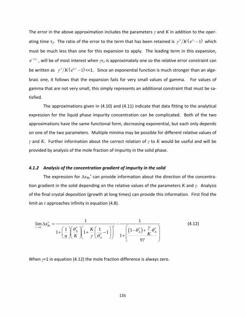
135

The error in the above approximation includes the parameters γ and K in addition to the oper-

ating time τ2. The ratio of the error to the term that has been retained is 22 1K e which

must be much less than one for this expansion to apply. The leading term in this expansion,

2e , will be of most interest when γτ2 is approximately one so the relative error constraint can

be written as 2 1 1K e <<1. Since an exponential function is much stronger than an alge-

braic one, it follows that the expansion fails for very small values of gamma. For values of

gamma that are not very small, this simply represents an additional constraint that must be sa-

tisfied.

The approximations given in (4.10) and (4.11) indicate that data fitting to the analytical

expression for the liquid phase impurity concentration can be complicated. Both of the two

approximations have the same functional form, decreasing exponential, but each only depends

on one of the two parameters. Multiple minima may be possible for different relative values of

γ and K. Further information about the correct relation of γ to K would be useful and will be

provided by analysis of the mole fraction of impurity in the solid phase.

4.1.2 Analysis of the concentration gradient of impurity in the solid

The expression for ΔxBcs can provide information about the direction of the concentra-

tion gradient in the solid depending on the relative values of the parameters K and γ. Analysis

of the final crystal deposition (growth at long times) can provide this information. First find the

limit as τ approaches infinity in equation (4.8).

* * *

*

1 1lim

1 1 11 1 11

s

Bc

A A A

A

x

KKK

(4.12)

When γ=1 in equation (4.12) the mole fraction difference is always zero.

136

** *

*

** **

1 1lim 1

11 1 11 1 1 11 1

1

1 10

1 111 11 1

s

bc

AA A

A

AA AA

xK

KK

KK

(4.13)

This indicates that, if the incorporation rate constants of A and B are the same, then there is no

concentration gradient in the crystal. A flat concentration profile in the crystal can only occur

when the ratio of A to B being added to the crystal remains constant at all times. This is true if

the total incorporation rate is constant. Therefore the driving force ratio of A to B must also be

constant for this result to be true and this was shown to be the case when γ =1 in section

2.4.1.2.

If K is equal to one, the following result is obtained.

* *

*

*

****

1 1lim 1

11 1 1 11 1 1 1

1 1

1 1 11 1 1 1 1 11 1 1

s

bc

A A

A

A

AAAA

x K

(4.14)

This indicates that even if the equilibrium behavior gives no separation in the solid phase, there

will be a concentration gradient in the crystal if the incorporation rate constants of A and B are

different. If γ is greater than one, then the final layer of crystal grown will have a smaller impur-

ity concentration than the initial layer. If γ is less than one, the final crystal layer will have more

impurity than the initial impurity layer.

It is also interesting to look at the cases where K and γ approach zero. The limit in the

case that either K or γ approaches zero of equation (4.8) is zero.

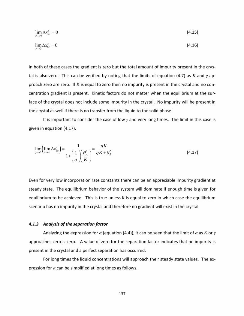
137

0lim 0s

bcK

x (4.15)

0lim 0s

bcx

(4.16)

In both of these cases the gradient is zero but the total amount of impurity present in the crys-

tal is also zero. This can be verified by noting that the limits of equation (4.7) as K and γ ap-

proach zero are zero. If K is equal to zero then no impurity is present in the crystal and no con-

centration gradient is present. Kinetic factors do not matter when the equilibrium at the sur-

face of the crystal does not include some impurity in the crystal. No impurity will be present in

the crystal as well if there is no transfer from the liquid to the solid phase.

It is important to consider the case of low γ and very long times. The limit in this case is

given in equation (4.17).

**0

1lim lim

11

s

bc

AA

Kx

K

K

(4.17)

Even for very low incorporation rate constants there can be an appreciable impurity gradient at

steady state. The equilibrium behavior of the system will dominate if enough time is given for

equilibrium to be achieved. This is true unless K is equal to zero in which case the equilibrium

scenario has no impurity in the crystal and therefore no gradient will exist in the crystal.

4.1.3 Analysis of the separation factor

Analyzing the expression for α (equation (4.4)), it can be seen that the limit of α as K or γ

approaches zero is zero. A value of zero for the separation factor indicates that no impurity is

present in the crystal and a perfect separation has occurred.

For long times the liquid concentrations will approach their steady state values. The ex-

pression for α can be simplified at long times as follows.

138

*

*

* *

11 1 1

1 1lim 1 1

1 11 1

A

A

A A

K

K

(4.18)

The best separations will occur for values of K and γ approaching zero. The behavior at

these limits can be approximated by taking a Taylor expansion of equation (4.18) about K=0

and γ=0. The derivation of the limit about γ=0 is described in section 6.1 . Keeping only first

order terms gives the following results.

2K K O K (4.19)

*

2

*

1ln 1

11

A

A

K

O

(4.20)

These limiting expressions indicate that the average concentration of the crystal phase

at long times are functions of the physical properties of the system; K, γ and θA*. In the case of

K approaching zero, the value of α becomes equal to K indicating that the separation factor is

determined by the equilibrium relationship between the solid and liquid phases. For γ ap-

proaching zero, the expression for α is more complicated and depends on all three physical pa-

rameters.

4.2 Batch Crystallization Experiments

Batch experiments were performed in order to provide data to validate and to fit para-

meter values to the previously defined model. The model has been developed for crystalliza-

tion occurring on fixed surfaces and so a method for doing this experimentally has been deter-

mined. The description of the experimental apparatus will be followed by discussion of the

chemical system used during experimentation and then the experimental results.

139

4.2.1 Experimental Apparatus

The necessary components of the experimental apparatus are a temperature controlled

solution of known initial composition and a fixed, temperature controlled surface upon which

crystal growth occurs. A means of taking samples from the liquid over the course of time and a

method for analyzing those samples are also required.

Experiments were conducted in a single-necked 100 mL round bottom flask submerged

in a constant temperature water bath. The constant temperature bath was maintained by cir-

culation from a Neslab RTE-1100 water circulator. The mixture was stirred with a magnetic stir

bar using a stir plate that allowed digital control of the rotation speed.

The crystallization solutions were made as follows. A measured amount of the compo-

nent of interest (A) and the impurity (B) were added to the round bottom flask along with 100 g

of water. This mixture was heated until the solids were dissolved. The temperature was then

cooled to the desired working temperature via the external water bath. During this heating and

cooling process, the growth surface was not present in the solution. The experiments were de-

signed such that the solution was not supersaturated at the bulk temperature. No nucleation

or growth would be expected until the seed plate is added to the solution.

The seeding device is a pre-coated length of metal tubing. The tube is bent into a U-

shape and pushed through a rubber septum that serves to seal the flask from the outside envi-

ronment. Both stainless steel and aluminum tubing was used with similar results. Aluminum

was chosen as a better material because it can be bent more smoothly to give a more uniform

seed surface.

The metal tube is made into a seed by evaporative coating from a saturated solution of

the component of interest. The tube is first lightly sanded using a rotary hand tool in order to

roughen the surface. The surface is then wiped with phosphoric acid in order to remove the

surface oxide layer and enhance wetting of the surface. The surface is then washed with water

to remove the acid and immediately is dipped into a saturated solution of the component of

interest. The tube is dipped three times in succession and then is allowed to dry in an 800C

oven. This coating process is then repeated 10-12 times or until a visible coating of solid is

present on the tube surface. The amount of solid deposited by this coating process is deter-

140

mined by weighing. The coating of seed that is developed is stable to mechanical agitation. A

picture of a coated seed tube is shown in Figure 50.

Figure 50. Picture of aluminum seed tube coated with asparagine.

The purpose of using metal tubing instead of a metal rod is temperature control of the

crystallization surface. Controlled temperature water is passed through the metal tube in order

to maintain the surface at a constant temperature. Initial experiments were done with no cool-

ing of the seed surface and a supersaturated initial solution. Although this approach did result

in preferential growth on the seed surface, most experiments also had a visible, significant

amount of bulk crystallization, due to secondary or homogeneous nucleation. Because the

purpose of the experiment is to study the impurity incorporation into crystal grown on a solid

surface bulk crystallization should be minimized. By cooling the seed surface, the bulk solution

can be kept at very small supersaturations or even slight undersaturation. This will eliminate

the possibility of homogeneous nucleation and will diminish the effects of secondary nucleation

because crystals that are dislodged from the growth surface can dissolve in the bulk solution.

141

The cooling of the seed surface is accomplished using a Netzsch NM011SY mini-

metering progressive cavity pump and a controlled temperature water bath. This pump was

connected to a DC motor and delivered a flow rate of 1.4 liters per minute at 500 RPM. The

controlled temperature water bath was capable of temperature control to within less than

0.10C. Fluid connections in the flow path from the pump through the seed loop are made using

double sleeved compression tube fittings.

A progressing cavity pump is a positive displacement pump that operates by moving flu-

id with a helical rotor turning inside of an elastomeric rubber stator. This rotation creates dis-

crete pockets of fluid that are moved through the pump. The stator is designed so that the

pockets start to overlap towards the discharge end of the pump in order to minimize pulsing

fluid flow.

The progressive cavity pump cavity pump is the best choice for this application because

it provides very smooth flow with a minimum of vibration. Vibrations are undesirable because

they propagate through the tubing and can result in oscillations of the seed tube. Oscillations

of the seed tube are expected to affect the amount of secondary nucleation arising from crys-

tals breaking away from the seed tube. Minimizing these oscillations is desired in order to sim-

plify experimental analysis.

Figure 51. Schematic of Nemo progressive cavity pump used during experimentation.151

142

The overall system is composed of the crystallization vessel, the seed tube with flow

loop and the temperature control system for the external bath. The inflow and outflow from

the Neslab chiller was not balanced and so an extra pump was necessary in order to deal with

overflow. A Cole-Parmer peristaltic pump was used for this purpose. A picture of the overall

experimental setup is given in Figure 52.

Figure 52. Experimental setup showing external temperature bath, crystallization flask and seed tube with at-tached tubing for surface temperature control.

Sampling of the liquid phase is accomplished by a needle inserted through the rubber

septum into the crystallization flask. The needle is left in the solution at all times and the end is

covered when liquid is not being extracted in order to limit solvent evaporation. To prepare

each sample, a volume of between 0.1 and 0.2 mL is taken from the solution. No more than 20

total samples were taken during a single experiment so that the total volume lost is less than 3

143

mL, or approximately 3 % of the total volume. Multiple samples were taken at some time

points in order to test the homogeneity of the solution.

From the liquid removed from the vessel, 0.1 mL is diluted with 4.9 g of water to give

the final sample to be analyzed for that time point. This level of dilution is used in order to op-

erate in an absorption regime far removed from the saturation limit of the UV-Vis detector.

The sample is taken via a calibrated pipette but the actual sample amount is also determined by

weighing in order to get more accurate data.

Accurate sample preparation is important because the concentrations involved are rela-

tively small and sampling errors can result in large uncertainties in the measured concentra-

tions. A 10% variance in sample volume leads to a roughly 10% change in the absorbance dur-

ing HPLC analysis via UV-Vis detection. But the overall change in absorbance from the feed to

the final solution for a typical experiment is often on the order to 10%. Careful sampling then is

very important.

Sampling of the solid phase was done by sequential dissolution. Once an experiment is

finished, the wet weight of the resulting crystal is recorded. The crystal was then air dried and

reweighed to give the dry product weight. Subsequent samples of the solid are collected by

placing the crystal in an unstirred vial of water for a specified period of time. The crystal was

then allowed to air dry before the weight was recorded. This process was repeated until the

entire crystal was dissolved. Air drying was used because oven drying was found to make the

crystal more brittle and prone to uneven dissolution.

This sampling method will be most appropriate when the crystal grown on the seed

plate is very uniform. The seed method used here does result in very uniform crystal growth

over the entire submerged surface of the seed tube. The product on the seed tube is not a sin-

gle crystal but a uniform, polycrystalline coating. A picture of the final crystal grown from one

experiment is shown in Figure 53.

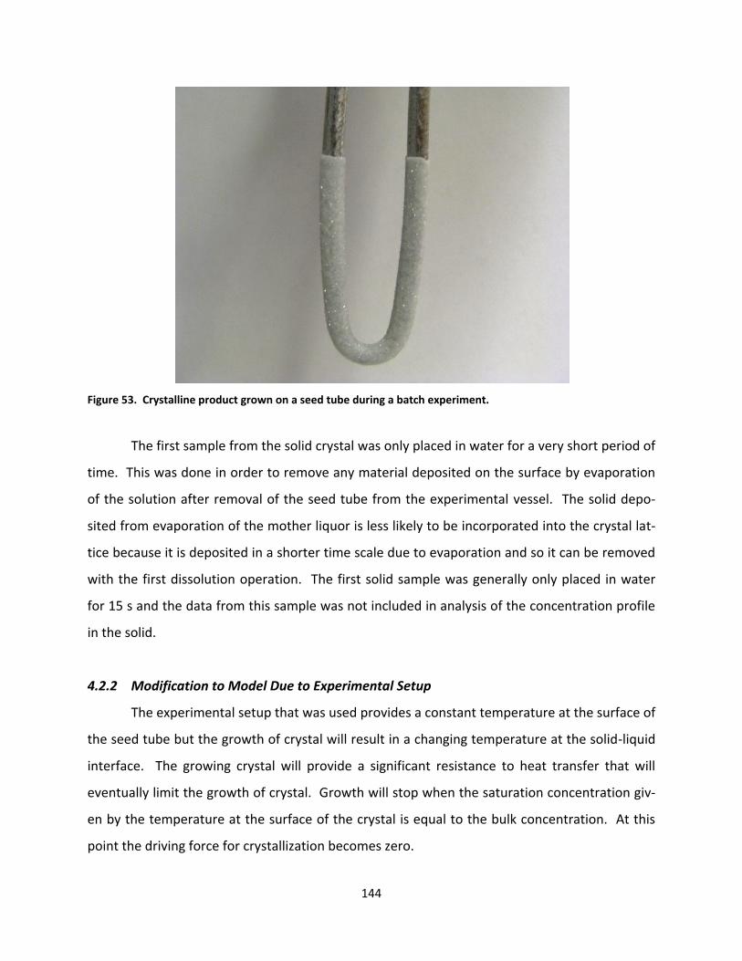
144

Figure 53. Crystalline product grown on a seed tube during a batch experiment.

The first sample from the solid crystal was only placed in water for a very short period of

time. This was done in order to remove any material deposited on the surface by evaporation

of the solution after removal of the seed tube from the experimental vessel. The solid depo-

sited from evaporation of the mother liquor is less likely to be incorporated into the crystal lat-

tice because it is deposited in a shorter time scale due to evaporation and so it can be removed

with the first dissolution operation. The first solid sample was generally only placed in water

for 15 s and the data from this sample was not included in analysis of the concentration profile

in the solid.

4.2.2 Modification to Model Due to Experimental Setup

The experimental setup that was used provides a constant temperature at the surface of

the seed tube but the growth of crystal will result in a changing temperature at the solid-liquid

interface. The growing crystal will provide a significant resistance to heat transfer that will

eventually limit the growth of crystal. Growth will stop when the saturation concentration giv-

en by the temperature at the surface of the crystal is equal to the bulk concentration. At this

point the driving force for crystallization becomes zero.

145

This changing surface temperature requires removal of one of the key assumptions

made when deriving the analytical solution above. Because the surface temperature is not con-

stant, the saturation concentration at that surface ( *

AC ) is also not constant. It is not required

that *

AC be constant to use the model defined earlier but it is necessary that its value be known

as a function of time. This can be accomplished by relating the temperature at the liquid-

crystal interface to the total mass of crystal present through an energy balance. This energy

balance will require estimation of heat transfer coefficients inside the seed tube and from the

bulk fluid to the surface of the seed tube in addition to a thermal conductivity for the crystal

layer. The shape of the growing crystal layer is also necessary and in this system will be cylin-

drical due to the use of tubing as the seed surface.

The varying temperature at the liquid-crystal surface is also expected to affect the val-

ues of the incorporation rate constant kA, the equilibrium constant K and the ratio of incorpora-

tion rate constants γ. Fitting of the model to experimental data will result in average values of

these parameters over the temperature range experienced at the growth surface. The value

determined from fitting the model to the experimental data will give an order of magnitude

understanding of these parameters but cannot give parameter values at specific temperatures

due to the experimental setup.

An energy balance over the system can be used to find the temperature at the surface

of the crystal as a function of time. The energy balance is done at quasi-steady state because

the growth rate of crystal is expected to be much slower than the time necessary to establish

thermal equilibrium. The total amount of energy transferred between the liquid inside the

seed tube and the bulk liquid will be constant because the water in the tube is at constant flow

rate and inlet temperature while the bulk temperature is also constant. The unknown variables

then are the total heat added to the seed tube and the temperatures at the interior surface of

the seed tube, the exterior surface of the seed tube and at the crystal surface.

For purposes of this energy balance, the system will be assumed to have the form

shown in Figure 54. In this figure the growth surface is a straight tube in the bulk solution. This

assumption eliminates consideration of the bends in the tube for interior heat transfer and as-

146

sumes the bulk solution is mixed well enough that the region between the U-shaped seed tube

legs has the same temperature as the bulk solution.

Figure 54. Diagram of heterogeneous batch crystallization system for energy balance purposes. Half of system is shown with mirror plane of symmetry at r=0. Tj and rj represent the temperature and radial distance at loca-tion j.

A heat transfer equation can be written for each of the four regions in Figure 54 (seed

tube interior, tube wall, crystal and bulk solution). These equations are presented in equations

(4.21) to (4.24).

1 1I I Iq h a T T (4.21)

1 1 22

1

2

ln

twLkq T T

rr

(4.22)

TB TS T2 T1 TI

r=0 r1 rS r2

Bulk Solution Crystal Tube

Wall

Seed Tube

Interior

147

2 2

2

2

ln

cS

S

Lkq T T

rr

(4.23)

B B c S Bq h a T T (4.24)

where qj is the heat transfer in watts of region j, hI is the heat transfer coefficient for the fluid

inside the seed tube to the tube wall, hB is the heat transfer coefficient from the bulk to the

crystal surface, ktw is the thermal conductivity of the tube wall, kc is the thermal conductivity of

the crystal, a1 is the interior surface area of the seed tube, ac is the surface area of the crystal

and L is the length of the seed tube submerged in the solution.

The thermal conductivity of the crystal layer is assumed to be equal to the thermal con-

ductivity of the component of interest. This is a good assumption because the impurity will on-

ly be present in a small quantity and in a solid solution the impurity will have a very similar

structure to the component of interest and cause only slight disturbance of the crystalline lat-

tice. The heat of crystallization released by growth of the crystal will be assumed small com-

pared to the heat transferred from the bulk liquid to the interior of the seed tube. This will be

demonstrated for the model system that will be described in the next section.

For a system at quasi steady state the heat transferred between two adjacent regions

will be equal. For the system outlined in Figure 54 and equations (4.21)-(4.24) all values of q

will be equal at steady state. The five unknown quantities then are q, T1, T2, TS and rS and the

four equations can be solved for the desired quantity TS as a function of the crystal thickness rS.

The expression for TS is presented in equation (4.25).

2

2 1 1

2

1 2 1 2 1 2 1

ln2 1

ln 2

ln2 21

ln ln ln

stwI B B c B B c

I c

S

stw tw twB c

I c

r rLkT T h a T h a

r r h a LkT

r rLk k Lkh a

h a r r k r r r r

(4.25)

148

The crystal thickness rS must be related to the solution phase concentrations in order for equa-

tion (4.25) to be used in the proposed model for batch crystallization. This is done by finding

the total mass of the crystal and using the conservation of mass in a batch system. The shape

of the crystal will be a cylindrical shell for the cylindrical seed tube used in these experiments.

0 0 0 0 2 2

2C AC BC A A B B A A B B C Sm m m m m m m V C C C C L r r (4.26)

Equation (4.26) can then be solved for rS which is given in equation (4.27).

0 0 2

2S A A B B

C

Vr C C C C r

L (4.27)

The remaining information needed to solve equation (4.25) is physical parameters of the

experimental setup and the chemical system in use. The thermal conductivities of the tube wall

and the crystal can be looked up while the values of r1, r2, L, TB, TI and a1 are known from the

established system materials and parameters and the surface area of the crystal, aC, can be re-

lated to rS ( 2C Sa r L ). The last two values that are required to solve for the temperature at

the crystal surface are the heat transfer coefficients from the bulk to the crystal surface and

from the interior to the wall of the seed tube.

The heat transfer coefficient inside the seed tube can be found from a correlation for

heat transfer inside a pipe. The submerged portion of the seed tube was in all cases at least 10

cm from the beginning of the seed tube. The inner diameter of the seed tube (D1) is 0.2 cm so

the ratio of length before the growth area to tube diameter is 50 and entrance effects can be

neglected. In order to choose the appropriate heat transfer correlation the Reynolds number

of the water flowing through the seed tube must be known. The volumetric flow rate in the

pipe (Q) is 1.4 liters per minute or 2.3 * 10-5 m3/s. The calculation of the Reynolds number is

shown in equation (4.28).

149

5

1

2 2 61

2.3*10 0.002Re 15000

0.001 10

QD

r

(4.28)

Where the kinematic viscosity of water (υ) at room temperature is 10-6 m2/s. This Reynolds

number is in the turbulent flow regime and the Dittus-Boelter correlation152 is appropriate.

0.8 0.41 0.023Re PrI

w

h DNu

k (4.29)

Pr is the Prandtl number of the fluid as defined in equation (4.30) and kw is the thermal conduc-

tivity of water which is equal to 0.58 W/mK. For the Prandtl number, the heat capacity at con-

stant pressure (cP), the viscosity (μ) and the thermal conductivity are all properties of the fluid.

Pr Pc

k

(4.30)

The Prandtl number for water at room temperature is approximately 7. The Nusselt number

for this situation is then equal to 110 which gives a heat transfer coefficient of 33,000 W/m2K

for transfer from the liquid flowing inside the seed tube to the surface of the seed tube. This

coefficient can only be considered constant throughout the entire seed tube if the flow rate

through the seed tube is high enough that the temperature change of the water from entrance

to exit of the seed tube is small. This temperature difference from inlet to outlet was measured

to be 0.250C so the assumption of constant internal heat transfer coefficient is reasonable.

The heat transfer coefficient from the bulk to the crystal surface was measured. Appro-

priate heat transfer correlations for stirred tank systems are difficult to find so a simple experi-

ment was done in order to measure this value for the conditions used during the batch crystal-

lization experiments. A piece of aluminum tubing, the same as used for seed tubing but with-

out any surface treatment, was inserted into a 100 mL solution of water held at 250C. Water

was passed through the tube from a controlled temperature water source and the inlet and

150

outlet temperatures from the aluminum tube were recorded. The same flow rate through the

seed tube used during crystallization experiments was used in order to find the most appropri-

ate heat transfer coefficient.

The measured inlet and outlet temperature along with the internal heat transfer coeffi-

cient from a correlation and the thermal conductivity of the aluminum tube allow for the bulk

heat transfer coefficient to be calculated. The total energy transfer is first found from the

change in temperature of the water during flow through the seed tube. This amount of heat

transfer is then used to find an overall heat transfer coefficient. The overall heat transfer coef-

ficient can then be used to find the bulk heat transfer coefficient. The equations for these three

steps are given in equation (4.31) to (4.33) where m is the mass flow rate of water in the seed

tube, cp is the heat capacity at constant pressure of water, Tout and Tin are the outlet and inlet

temperatures respectively of the water in the feed tube, q is the heat transfer in watts, lmT is

the log mean temperature difference between the water in the seed tube and the bulk, and a2

is the outside surface area of the seed tube.

p out inq mc T T (4.31)

2O lmq U a T (4.32)

2 12 2

1

1

ln1 1

2

O

B tw I

UD DD D

h k D h

(4.33)

For the previously discussed flow rate of 1.4 liters per minute and a bath temperature of 100C

the temperatures of water entering and exiting the seed tube are 11.38 and 11.620C respective-

ly. This corresponds to heat transfer (q) of 31 W and a bulk heat transfer coefficient equal to

3,100 W/m2K.

The values of the heat transfer coefficients and equation (4.25) can be added to the

batch model outlined in section 2.2 in order to allow numeric simulation of the proposed batch

experiments. The collected experimental data can then be fit to this model using a least

squares approach in order to give values for the model parameters , Ak and K .

151

4.2.3 Model Chemical System

The chemical system chosen for experimentation was the amino acids asparagine and

aspartic acid in water. The structures of asparagine (asn) and aspartic acid (asp) are shown in

Figure 55.

O

OH

NH2

O

NH2

O

OH

OH

O

NH2

Asparagine Aspartic Acid

Figure 55. Structure of the amino acids asparagine and aspartic acid.

It has been previously found153, 154 that asparagine and aspartic acid form a solid solu-

tion with up to 20% by weight of aspartic acid in the asparagine crystalline lattice. The forma-

tion of a solid solution was also verified experimentally for the range of concentrations of inter-

est in this study. The details of this are given in section 6.5. The similar shape of these two mo-

lecules also supports the formation of a solid solution.

Another benefit of asparagine as the component of interest is that it exhibits a strongly

temperature dependent solubility in water149. The strong dependence on temperature allows

for larger amounts of crystal to be grown with smaller temperature differences. This is impor-

tant because in this system only a small amount of impurity is present in the crystal and larger

total amounts of crystal facilitate concentration measurement.

Both asparagine and aspartic acid crystallize as a mono-hydrate. This means that the

crystal structure of pure asparagine or aspartic acid will contain one water molecule for every

molecule of asparagine or aspartic acid. The solid solution formed between asparagine and as-

partic acid will also be a mono-hydrate.

Because the solubility of these amino acids in water is small the amount of water in the

crystal is also small and will not affect the concentration of the liquid phase. Every gram of as-

paragine crystal will contain 0.14 g of water. The saturation of asparagine at 200C is roughly 2 g

asparagine per 100 g water. If the initial solution has a supersaturation ratio of 1.5 and the

crystallization proceeds to equilibrium then 1 gram of crystal will form containing 0.14 g water.

152

The change in the amount of water present will be 0.1%. The assumption in the batch model

development that the amount of solvent in the liquid phase was constant will still be appropri-

ate.

The presence of a mono-hydrate can explain why oven drying is not a good strategy

when analyzing the solid crystals of asparagine and aspartic acid. High temperatures allow the

bound water in the crystal matrix to evaporate which results in a significant change in the sta-

bility of the crystal. The crystal becomes very brittle and prone to breaking off in large pieces

which makes uniform sampling of the crystal very difficult. Air drying allows surface moisture

to evaporate without removing water from the crystalline lattice so that the crystal does not

become brittle.

The heat of crystallization for asparagine monohydrate is 33 kJ/mol155. For the same

conditions discussed previously, 1 g of asparagine crystal will require 250 J of energy for crystal-

lization. If this growth is spread out over the course of one hour a power input of 0.07 W will

be required. This growth will in fact generally be spread over multiple hours decreasing the ne-

cessary power even further. This heat input is much less than the heat transfer from the cool-

ing loop to the bulk solution in the batch experimental setup and so the assumption that the

heat of crystallization can be ignored is justified.

Asparagine and aspartic acid were purchased from Sigma-Aldrich at 99.5% purity and

used without further purification.

4.2.4 Estimation of Maximum Mass Transfer Rate

The estimated outside heat transfer coefficient allows estimation of a mass transfer

coefficient for asparagine and aspartic acid in water by use of the Chilton-Colburn analogy.156,

157 This relationship is given by

2 23 3St Pr St Scm (4.34)

where St is the Stanton number, Pr is the Prandtl number, Stm is the mass transfer Stanton

number and Sc is the Schmidt number. These dimensionless variables are defined as follows.

153

St=p

h

Vc (4.35)

St = mm

h

V (4.36)

Pr=pc

k

(4.37)

Sc=ijD

(4.38)

where h is the heat transfer coefficient (W/m2 K), ρ is the density of the fluid (kg/m3), V is the

fluid velocity (m/s), cp is the heat capacity at constant pressure (J/kg K), hm is the mass transfer

coefficient (m/s), μ is the viscosity (kg/m s), k is the thermal conductivity (W/m K), ν is the ki-

nematic viscosity (m2/s) and Dij is the diffusivity of j in i (m2/s).

Equation (4.34) can be rearranged to give the following expression for the mass transfer

coefficient.

23Pr

Scm

p

hh

c

(4.39)

The only unknown parameter in equation is the Schmidt number. The heat transfer

coefficient was found in the last section to be 3,100 W/m2K and the density of water is approx-

imately 1,000 kg/m3, the heat capacity at constant pressure of water is 4,183 J/kg K, and the

Prandtl number of water is 7 at room temperature. Also, the kinematic viscosity of water is 10-6

m2/s so the only unknown quantity is the diffusivity of asparagine or aspartic acid in water. The

diffusivity can be estimated using the Hayduk-Laudie correlation158 which is given in the follow-

ing equation.

5

1.14 0.589

13.16*10wA

w A

DV

(4.40)

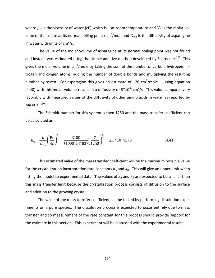
154

where μw is the viscosity of water (cP) which is 1 at room temperature and VA is the molar vo-

lume of the solute at its normal boiling point (cm3/mol) and DwA is the diffusivity of asparagine

in water with units of cm2/s.

The value of the molar volume of asparagine at its normal boiling point was not found

and instead was estimated using the simple additive method developed by Schroeder.159 This

gives the molar volume in cm3/mole by taking the sum of the number of carbon, hydrogen, ni-

trogen and oxygen atoms, adding the number of double bonds and multiplying the resulting

number by seven. For asparagine this gives an estimate of 126 cm3/mole. Using equation

(4.40) with this molar volume results in a diffusivity of 8*10-6 cm2/s. This value compares very

favorably with measured values of the diffusivity of other amino acids in water as reported by

Ma et al.160

The Schmidt number for this system is then 1250 and the mass transfer coefficient can

be calculated as

2 23 3

5Pr 3100 72.3*10 /

Sc 1000 4183 1250m

p

hh m s

c

(4.41)

This estimated value of the mass transfer coefficient will be the maximum possible value

for the crystallization incorporation rate constants kA and kB. This will give an upper limit when

fitting the model to experimental data. The values of kA and kB are expected to be smaller than

this mass transfer limit because the crystallization process consists of diffusion to the surface

and addition to the growing crystal.

The value of the mass transfer coefficient can be tested by performing dissolution expe-

riments on a pure species. The dissolution process is expected to occur entirely due to mass

transfer and so measurement of the rate constant for this process should provide support for

the estimate in this section. This experiment will be discussed with the experimental results.

155

4.2.5 Concentration Measurements

All concentration measurements were done using high pressure liquid chromatography

(HPLC). The instrument used was an Agilent 1200 series HPLC with a diode array detector.

Amino acids are not directly detectible by UV/Vis spectroscopy so a pre-column derivatization

reaction is necessary before analysis. The amino acids are reacted with ortho-phthalaldehyde

(OPA) in the presence of 3-mercaptopropionic acid. This reaction is shown in Figure 56. The

functionalized amino acids produced in this reaction are unstable and reproducibility of the de-

rivatization method is very important in order to compare data between samples.161 This deri-

vatization reaction can be carried out automatically by the Agilent 1200 series auto-sampler in a

reproducible manner.

H

H

O

O

OH

O

R

NH2

SH OH

O

N

S

OH

O

OH

R

O

+ +

Figure 56. Schematic of reaction of primary amino acid with o-phthalaldehyde in the presence of 3-mercaptopropionic acid to give a derivative detectable with absorbance spectroscopy.

A HPLC method for separating amino acids published by the Agilent Corporation was

used as the basis for the experimental method in this investigation162. The separation is done

using a gradient elution profile with two solvents. Solvent A is 5 mM sodium phosphate and 5

mM sodium borate in water with the pH adjusted to 8.2. Solvent B is a 45:45:10 mixture of ace-

tonitrile, methanol and water. The gradient conditions are shown in Figure 57 as the percen-

tage of solvent B as a function of time for a total flow rate of 1 mL/min. Each HPLC measure-

ment takes a total of 14.5 minutes. Data are collected during the first 8.4 minutes while the last

6.1 minutes are used for re-equilibration of the column and for preparation of the next sample

in the autosampler. The program used by the autosampler is detailed in Table 2.

156

Figure 57. Percentage of solvent B in HPLC effluent vs. time for separation of amino acids asparagine and aspar-tic acid.

Table 2. Autosampler program used with the Agilent 1200 autosampler in order to perform pre-column deriva-tization reaction of amino acids with o-phthalaldehyde. Mixing of syringe contents is done by moving the injec-tor piston back and forth in air.

0

10

20

30

40

50

60

70

80

90

100

0 5 10 15

% o

f S

olv

ent

B

Time (min)

1. Draw 2.5 μL borate buffer into syringe.

2. Draw 0.5 μL 1 mM valine solution into syringe.

3. Draw 0.5 μL sample into syringe.

4. Mix syringe contents 5 times.

5. Wait 0.2 minutes.

6. Draw 0.5 μL OPA solution into syringe.


8. Draw 32 μL water into syringe.


10. Inject syringe contents onto column.

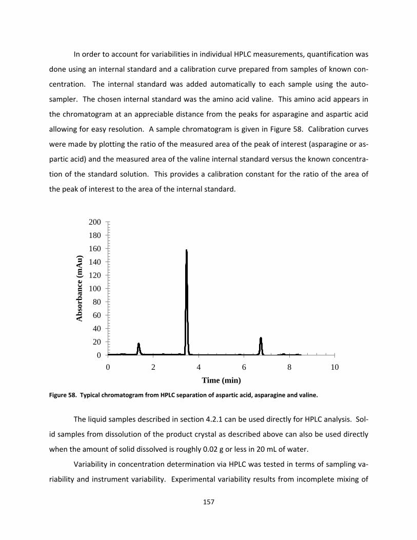
157

In order to account for variabilities in individual HPLC measurements, quantification was

done using an internal standard and a calibration curve prepared from samples of known con-

centration. The internal standard was added automatically to each sample using the auto-

sampler. The chosen internal standard was the amino acid valine. This amino acid appears in

the chromatogram at an appreciable distance from the peaks for asparagine and aspartic acid

allowing for easy resolution. A sample chromatogram is given in Figure 58. Calibration curves

were made by plotting the ratio of the measured area of the peak of interest (asparagine or as-

partic acid) and the measured area of the valine internal standard versus the known concentra-

tion of the standard solution. This provides a calibration constant for the ratio of the area of

the peak of interest to the area of the internal standard.

Figure 58. Typical chromatogram from HPLC separation of aspartic acid, asparagine and valine.

The liquid samples described in section 4.2.1 can be used directly for HPLC analysis. Sol-

id samples from dissolution of the product crystal as described above can also be used directly

when the amount of solid dissolved is roughly 0.02 g or less in 20 mL of water.

Variability in concentration determination via HPLC was tested in terms of sampling va-

riability and instrument variability. Experimental variability results from incomplete mixing of

0

20

40

60

80

100

120

140

160

180

200

0 2 4 6 8 10

Ab

sorb

an

ce (

mA

u)

Time (min)

158

the liquid phase and from small crystals present in solution that dissolve upon dilution of the

liquid sample while instrument variability can arise from the uncertainty for volume measure-

ment in the syringe.

The variability due to the Agilent instrument was tested by performing multiple injec-

tions of the same sample. The injection-to-injection variability in peak area ratio of asparagine

to valine was found to be 1.7 + 1.3 % for asparagine and 1.4 + 1.3 % for the aspartic acid to va-

line area ratio. Variability due to sampling was tested by taking two samples at one time point

and comparing the resulting HPLC areas. The variability due to sampling was found to be 1.7 +

1.7% for the asparagine to valine and 2.8 + 2.8% for aspartic acid to valine area ratio. The sam-

pling variability is then indistinguishable from the instrument variability and in both cases the

amount of variability is small.

4.3 Experimental Results and Discussion

4.3.1 Experimental Results

Experiments were performed at three different temperatures of the controlled temper-

ature water bath used for cooling of the seed tube in order to explore the effect of temperature

on the impurity incorporation during batch growth. Three experiments were performed at

each of these temperatures in order to test the reproducibility of the proposed experimental

method.

The initial concentrations of asparagine and aspartic acid were held constant in these

experiments at 2.6 g of asparagine and 0.4 g of aspartic acid in 100.0 g of water. The concen-

tration of asparagine was chosen so that the asparagine super-saturation at the bulk tempera-

ture of 250C is roughly zero. Industrial crystallizations can have a wide range of impurity con-

centrations. The mass ratio of aspartic acid to asparagine in these experiments is 8 % which is a

reasonable value for the impurity concentrations in industrial crystallization.

All experiments were conducted with a stirring rate of 200 rpm using a magnetic stir bar

with a length of 1 inch. The pump was operated at 500 rpm for all experiments resulting in a

flow rate of water through the seed tube of 1.4 liters per minute. The duration of each experi-

ment was between 8 and 10 hours.

159

The overall mass balance for each experiment was checked by taking the known initial

amounts of asparagine and aspartic acid and subtracting the weighed amount of crystal prod-

uct and the final amounts in the liquid phase as determined by HPLC. Mass balances on aspa-

ragine and aspartic acid were performed as well by using HPLC analysis of the solid phase to

determine the amount of each species that was deposited.

The discrepancy between mass in and the measured mass out is the accumulation. This

can also be measured directly with the following procedure. After the seed tube with product

is removed from the crystallization vessel, the vessel is sealed and heated before additional

samples are taken for HPLC analysis. The purpose of this operation is to measure the amount of

solid material present on surfaces other than the seed tube; such as the stir bar or the vessel

walls. A large amount of solid being deposited on surfaces other than the seed tube could inva-

lidate model fitting to the liquid phase concentration data.

The error in the mass balance will be compared to the initial amount of material used

and also to the amount of crystal grown. The amount of crystal grown will be small in relation

to the initial amount of material so a small percentage error in relation to the initial amount of

material will be a much larger error in relation to the amount of product.

The liquid phase concentration and the solid phase impurity mole fraction data are fit-

ted to the model using least squares regression. The batch model developed in section 2.2

along with the modification for non-constant surface temperature from section 4.2.2 were used

with MATLAB to find the parameter values that provide the best fit of the measured data. The

liquid phase concentration data are fit first to give a value for kA, γ and K. The asparagine con-

centration data are used to fit kA and the aspartic acid concentration data are then used with

the value of kA to fit γ and K. The values of kA fitted to the asparagine liquid phase data are

then used with the solid phase data to find values of γ and K from the solid phase dissolution

measurements.

Because the model has been modified to account for a variable temperature at the crys-

tal-liquid interface the concentration of asparagine does depend slightly on the parameters γ

and K. The total amount of crystal depends on the parameters γ and K and the surface tem-

perature depends on the total amount of crystal. In order to account for this the parameter

160

fitting is iterated until the difference in parameter values between sequential fittings is less

than 0.1% of the value from the newest fit. Fitting of the solid phase data are done after this

iterative fitting so that the final value of kA is used when fitting the solid phase data.

A plot representing one experiment is presented for each of the three temperatures of

the seed tube water source. Each plot will show the measured concentration data as a function

of time along with the best fit curve generated from model fitting to the data for that individual

experiment. Reported values of the fitted parameters for each seed tube water source tem-

perature represent averages over multiple experiments.

4.3.1.1 Experiments with a seed tube water source temperature of 50C

The first set of experiments was conducted with the seed tube water source tempera-

ture at 50C. The temperature at the inlet to the seed tube under these conditions was 7.00C

and the temperature at the outlet of the feed tube was 7.30C. The concentration vs. time data

along with best fit curves are shown in Figure 59 and Figure 60 for asparagine and aspartic acid

respectively. The solid phase data collected by sequential dissolution of the crystal grown on

the seed tube is presented in plots of mole fraction of aspartic acid versus relative mass of crys-

tal. The relative mass of crystal is the mass of crystal from the seed tube wall to the point of

measurement normalized by the total mass of crystal grown. A value of zero corresponds to

the beginning of crystallization at the seed tube surface and a value of one is the exposed sur-

face of the grown crystal. Samples are collected starting from a relative mass of one and pro-

ceeding towards zero. The solid phase data and best fit curve for the same experiment shown

in Figure 59 and Figure 60 are shown in Figure 61.

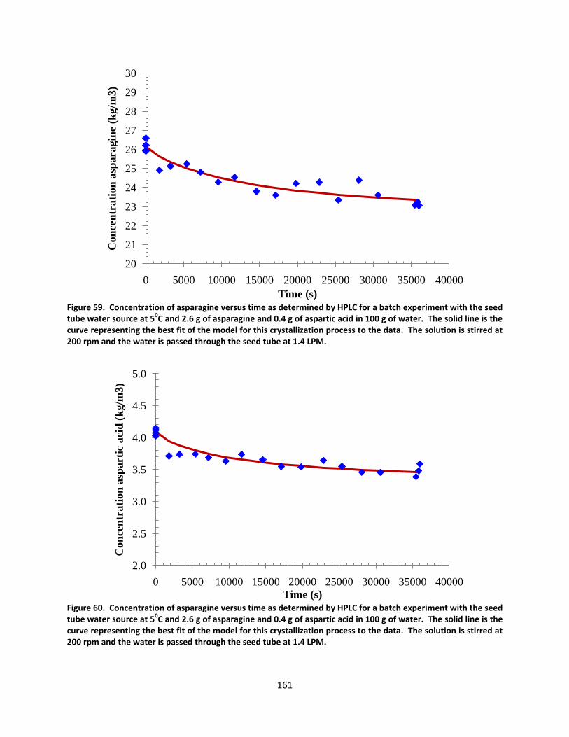
161

Figure 59. Concentration of asparagine versus time as determined by HPLC for a batch experiment with the seed tube water source at 50C and 2.6 g of asparagine and 0.4 g of aspartic acid in 100 g of water. The solid line is the curve representing the best fit of the model for this crystallization process to the data. The solution is stirred at 200 rpm and the water is passed through the seed tube at 1.4 LPM.


20

21

22

23

24

25

26

27

28

29

30

0 5000 10000 15000 20000 25000 30000 35000 40000

Con

cen

trati

on

asp

ara

gin

e (k

g/m

3)

Time (s)

2.0

2.5

3.0

3.5

4.0

4.5

5.0

0 5000 10000 15000 20000 25000 30000 35000 40000

Con

cen

trati

on

asp

art

ic a

cid

(k

g/m

3)

Time (s)

162

Figure 61. Mole fraction of aspartic acid versus relative crystal mass as determined by HPLC for a batch experi-ment with the seed tube water source at 50C and 2.6 g of asparagine and 0.4 g of aspartic acid in 100 g of water. The dashed line is the curve representing the best fit of the model for this crystallization process to the data. The solution is stirred at 200 rpm and the water is passed through the seed tube at 1.4 LPM.

The average values of the parameters , Ak and K for experiments with the cold water

source at 50C are listed in Table 3 along with the average yield of asparagine, the average

amount of crystal grown and the average accumulation in the liquid phase for these experi-

ments. The yield is the weighed amount of product on the seed tube divided by the initial

amount of asparagine and the accumulation is determined by the difference between the con-

centration of the heated solution remaining after the seed tube is removed and the final con-

centration of the liquid phase as determined by HPLC.

0.04

0.05

0.06

0.07

0.08

0.09

0.10

0 0.2 0.4 0.6 0.8 1

Mole

Fra

ctio

n A

spart

ic A

cid

Relative Crystal Mass

163

Phase kA (m/s) γ K Yield (%) Product (g) Accumulation (g)

2.9 + 1.2*10-6 9.7 + 0.3 0.252 + 0.008 0.10 + 0.04

Liquid 11 + 4 1.2 + 0.1

Solid 3.3 + 3.2 0.49 + 0.04

Table 3. Average experimentally determined values for parameters kA, γ and K along with the yield of aspara-gine, the mass of product and the mass of accumulation in the system for experiments with starting amounts of 2.6 g of asparagine, 0.4 g aspartic acid in 100 g water, stirred at 200 rpm with water flowing through the seed tube at 1.4 LPM with a seed tube water source temperature of 50C. Parameters γ and K were determined from both liquid and solid phase data.


The next set of experiments used a cold source temperature of 100C. The temperature

at the inlet and outlet of the seed tube was 11.40C and 11.60C respectively. The concentration

vs. time data for asparagine and aspartic acid are shown in Figure 62 and Figure 63 while the

mole fraction aspartic acid in the crystal as a function of relative mass is given in Figure 64.


20

21

22

23

24

25

26

27

28

29

30

0 5000 10000 15000 20000 25000 30000 35000 40000

Con

cen

tra

tion

asp

ara

gin

e (k

g/m

3)

Time (s)

164

Figure 63. Concentration of aspartic acid versus time as determined by HPLC for a batch experiment with the seed tube water source at 100C and 2.6 g of asparagine and 0.4 g of aspartic acid in 100 g of water. The solid line is the curve representing the best fit of the model for this crystallization process to the data. The solution is stirred at 200 rpm and the water is passed through the seed tube at 1.4 LPM.

Figure 64. Mole fraction of aspartic acid versus relative crystal mass as determined by HPLC for a batch experi-ment with the seed tube water source at 100C and 2.6 g of asparagine and 0.4 g of aspartic acid in 100 g of wa-ter. The dashed line is the curve representing the best fit of the model for this crystallization process to the da-ta. The solution is stirred at 200 rpm and the water is passed through the seed tube at 1.4 LPM.

2.0

2.5

3.0

3.5

4.0

4.5

5.0

0 5000 10000 15000 20000 25000 30000 35000 40000

Con

cen

trati

on

asp

art

ic a

cid

(k

g/m

3)

Time (s)

0.04

0.05

0.06

0.07

0.08

0.09

0.10

0 0.2 0.4 0.6 0.8 1

Mole

Fra

ctio

n A

spart

ic A

cid


165

The average values of the parameters , Ak and K for experiments with the cold water

source at 100C are listed in Table 4 along with the average yield of asparagine, amount of prod-

uct and amount of accumulation for these experiments.


1.4 + 0.4*10-6 5.6 + 0.8 0.15 + 0.02 0.14 + 0.05

Liquid 13 + 10 3.3 + 2.4

Solid 0.63 + 0.22 0.53 + 0.04



Experiments were also conducted using a cold source temperature of 150C. The tem-

perature at the inlet and outlet of the seed tube was 16.40C and 16.60C respectively. The con-

centration vs. time data for asparagine and aspartic acid are shown in Figure 65 and Figure 66

while the mole fraction aspartic acid in the crystal as a function of relative mass is given in Fig-

ure 67. The average values of the parameters , Ak and K for experiments with the cold wa-

ter source at 150C are listed in Table 4 along with the average yield of asparagine, amount of

product and amount of accumulation for these experiments.

166


Figure 66. Concentration of aspartic acid versus time as determined by HPLC for a batch experiment with the seed tube water source at 150C and 2.6 g of asparagine and 0.4 g of aspartic acid in 100 g of water. The solid line is the curve representing the best fit of the model for this crystallization process to the data. The solution is stirred at 200 rpm and the water is passed through the seed tube at 1.4 LPM.

20

21

22

23

24

25

26

27

28

29

30

0 5000 10000 15000 20000 25000 30000 35000 40000

Con

cen

trati

on

asp

ara

gin

e (k

g/m

3)

Time (s)

2.0

2.5

3.0

3.5

4.0

4.5

5.0

0 5000 10000 15000 20000 25000 30000 35000 40000

Con

cen

trati

on

asp

art

ic a

cid

(k

g/m

3)

Time (s)

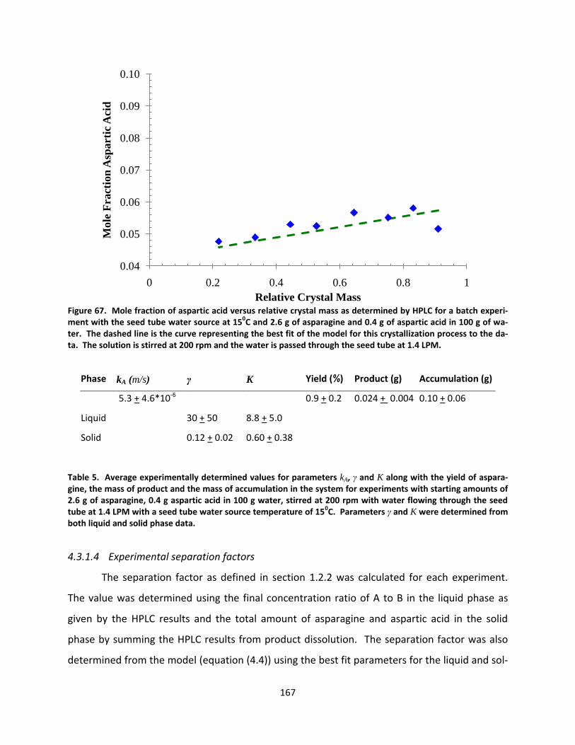
167

Figure 67. Mole fraction of aspartic acid versus relative crystal mass as determined by HPLC for a batch experi-ment with the seed tube water source at 150C and 2.6 g of asparagine and 0.4 g of aspartic acid in 100 g of wa-ter. The dashed line is the curve representing the best fit of the model for this crystallization process to the da-ta. The solution is stirred at 200 rpm and the water is passed through the seed tube at 1.4 LPM.


5.3 + 4.6*10-6 0.9 + 0.2 0.024 + 0.004 0.10 + 0.06

Liquid 30 + 50 8.8 + 5.0

Solid 0.12 + 0.02 0.60 + 0.38


4.3.1.4 Experimental separation factors

The separation factor as defined in section 1.2.2 was calculated for each experiment.

The value was determined using the final concentration ratio of A to B in the liquid phase as

given by the HPLC results and the total amount of asparagine and aspartic acid in the solid

phase by summing the HPLC results from product dissolution. The separation factor was also

determined from the model (equation (4.4)) using the best fit parameters for the liquid and sol-

0.04

0.05

0.06

0.07

0.08

0.09

0.10

0 0.2 0.4 0.6 0.8 1

Mole

Fra

ctio

n A

spart

ic A

cid


168

id phase data. The average calculated values of the separation factor are shown in Table 6 for

the three seed tube water source temperatures used.

Seed Tube Water Source Temperature (0C) αexp αL,fit αS,fit

5

10

15

0.60 + 0.04

0.57 + 0.05

0.6 + 0.2

1.6 + 0.2

2.7 + 0.6

10 + 7

0.55 + 0.03

0.54 + 0.03

0.32 + 0.09

Table 6. Separation factors as a function of seed tube water source temperature from experimental data (αexp) and from the batch model using the best fit parameters for both the liquid (αL,fit) and solid (αS,fit) phase experi-mental data. Data was collected for experiments with 2.6 g of asparagine, 0.4 g aspartic acid in 100 g water, stirred at 200 rpm with water flowing through the seed tube at 1.4 LPM with a seed tube water source tempera-ture of 5, 10 or 150C.

4.3.1.5 Experiments with pure asparagine

Experiments were performed with pure asparagine in order to determine the dissolu-

tion rate for asparagine. These experiments were performed by taking a seed tube with pure

asparagine crystal and submerging it in a stirred solution of water at 250C. The pure asparagine

coated seed tube was obtained by performing an experiment similar to the ones described

above with no aspartic acid. No water is passed through the seed tube during this operation.

Samples are then taken with time and the concentration is determined by HPLC analysis.

The dissolution is limited by the amount of crystal on the seed tube which rapidly ap-

proaches zero for the large driving forces used in these experiments. The dissolution rate is es-

timated using only the first few data points to approximate the tangent to the dissolution pro-

file. The temperature during this dissolution experiment is constant and so data fitting is done

to the simple equation given in equation (2.32). A graph of one experiment along with the fit-

ted tangent line is given in Figure 68.

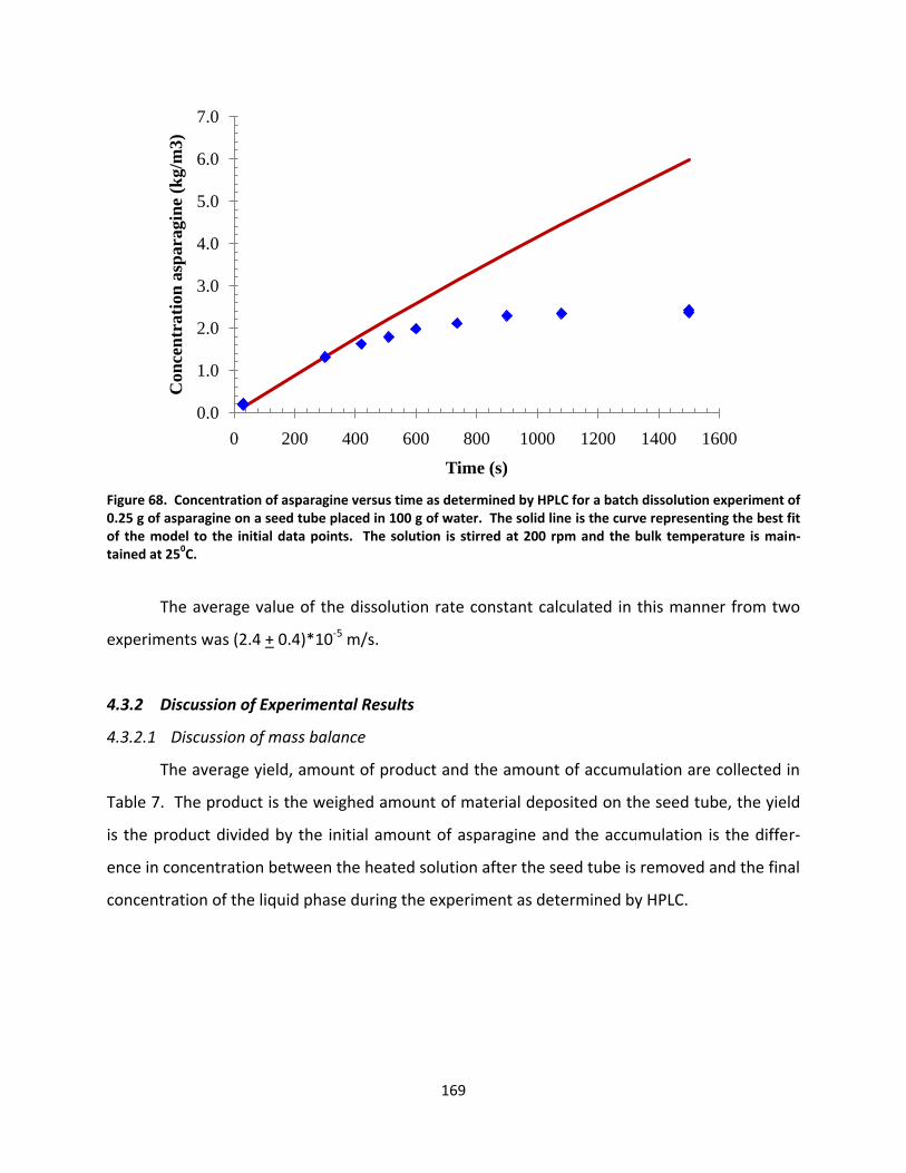
169

Figure 68. Concentration of asparagine versus time as determined by HPLC for a batch dissolution experiment of 0.25 g of asparagine on a seed tube placed in 100 g of water. The solid line is the curve representing the best fit of the model to the initial data points. The solution is stirred at 200 rpm and the bulk temperature is main-tained at 250C.

The average value of the dissolution rate constant calculated in this manner from two

experiments was (2.4 + 0.4)*10-5 m/s.

4.3.2 Discussion of Experimental Results

4.3.2.1 Discussion of mass balance

The average yield, amount of product and the amount of accumulation are collected in

Table 7. The product is the weighed amount of material deposited on the seed tube, the yield

is the product divided by the initial amount of asparagine and the accumulation is the differ-

ence in concentration between the heated solution after the seed tube is removed and the final

concentration of the liquid phase during the experiment as determined by HPLC.

0.0

1.0

2.0

3.0

4.0

5.0

6.0

7.0

0 200 400 600 800 1000 1200 1400 1600

Con

cen

trati

on

asp

ara

gin

e (k

g/m

3)

Time (s)

170

Seed Tube Water Source Temperature (0C) Yield (%) Product (g) Accumulation (g)

5

10

15

9.7 + 0.3

5.6 + 0.8

0.9 + 0.2

0.252 + 0.008

0.15 + 0.02

0.024 + 0.004

0.10 + 0.04

0.14 + 0.05

0.10 + 0.06

Table 7. Average experimentally determined values for yield (in relation to initial amount of asparagine), prod-uct and accumulation for experiments with 2.6 g of asparagine, 0.4 g aspartic acid in 100 g water, stirred at 200 rpm with water flowing through the seed tube at 1.4

It is apparent from Table 7 that the amount of accumulation in the liquid phase during

these experiments is of the same order of magnitude as the total amount of product generated

in these experiments. This means that the concentration depletion in the liquid phase is caused

by a significant amount of crystallization on surfaces other than the seed tube. Fitting of the

model parameters to the liquid phase concentration profiles will result in significant overesti-

mation because of this extra crystallization occurring in the liquid phase.

Even though the amount of accumulation is comparable to the amount of crystal grown

on the seed tube the overall mass balance with respect to the initial amounts of material in all

cases has less than 10% error. This is possible because the overall change in concentration of

the liquid phase is small compared to the initial concentrations. The amount of material (aspa-

ragine and aspartic acid) at the beginning of every experiment is 3 g. For one experiment per-

formed with the seed tube water source temperate at 50C the total amount of material in the

liquid phase and on the seed tube at the end of the experiment as determined by HPLC and

weighing was 2.9 g. The 0.1 g difference corresponds to a 3% error in relation to the total initial

mass but in relation to the 0.25 g of product grown on the seed tube this is a 40 % error. The

concentration profile in the liquid then represents 40% more depletion of material than is ac-

counted for on the seed tube surface and so a large error in the parameters fitted to the liquid

phase data is expected.

A larger ratio of crystal grown to accumulation in the liquid phase is necessary to obtain

reasonable parameters from liquid phase concentration data. This could be done by increasing

the amount of crystal growth if the accumulation stays constant or by decreasing the amount of

171

accumulation. More growth could be obtained by increasing the surface area for growth or in-

creasing the supersaturation. The supersaturation can be increased by lowering the tempera-

ture of the water flowing through the seed tube or by increasing the initial concentration. In-

creasing the initial concentration though is not expected to be a good approach to this problem

because higher concentrations of the bulk liquid will increase the possibility of nucleation in the

bulk and it will likely not address the issue of the total growth being small compared to the ini-

tial amount of material.

Lowering the temperature in the seed tube is a good option because the bulk tempera-

ture and concentration remain the same but more growth will occur on the seed tube. This is

seen for the experiments conducted here with the lowest temperature of water flowing

through the seed tube loop. These experiments correspond to the largest amount of product

and the smallest ratio of accumulation to product. In fact the accumulation is roughly constant

for the experiments at the three different seed tube water source temperatures which if true

for even lower temperatures of the seed tube water source would support this strategy.

The accumulation may depend on the stirring speed or the bulk temperature. Raising

the temperature of the bulk liquid may help to reduce accumulation in the liquid phase but this

would also likely result in smaller amounts of crystal growth for a fixed temperature in the seed

tube so this strategy should be pursued in conjunction with a lower seed tube water tempera-

ture. Experiments varying the bulk temperature and the stirring speed may provide insight that

would allow accumulation to be minimized by appropriate choices of the operating parameters.

Both of these parameters also are expected to have an impact on the kinetic parameters of the

crystallization and this must be accounted for as well when attempting to minimize accumula-

tion.

4.3.2.2 Discussion of fitted parameters

The fitted parameters for the three different seed tube water source temperatures are

listed again in Table 8.

172

Liquid Phase Solid Phase

Seed Tube Water Source Temperature (0C)

kA*106 (m/s) γ K γ K

5 2.9 + 1.2 11 + 4 1.2 + 0.1 3.3 + 3.2 0.49 + 0.04

10 1.4 + 0.4 13 + 10 3.3 + 2.4 0.63 + 0.22 0.53 + 0.04

15 5.3 + 4.6 30 + 50 8.8 + 5.0 0.12 + 0.02 0.60 + 0.38

Table 8. Average experimentally determined values for the parameters kA, γ and K for experiments with 2.6 g of asparagine, 0.4 g aspartic acid in 100 g water, stirred at 200 rpm with water flowing through the seed tube at 1.4 LPM with a seed tube water source temperature of 5, 10 or 150C. Parameters γ and K were determined from both liquid and solid phase data.

The experimental method used complicates the interpretation of these average para-

meter values. The model parameters are expected to depend on temperature so the fitted val-

ues from these experiments are an average over the temperature range experienced at the liq-

uid-solid interface. The fitted parameters from these experiments then do not represent the

parameter values at a specific temperature which would be the most useful information for

modeling purposes. The fitted values can be used to understand the magnitude of the con-

stants which is very important because the value of γ in relation to one has a significant impact

on the utility of the proposed counter-current process as seen in section 2.4.

The bulk temperature in all experiments was held at the same value so that there is

overlap in the temperature range experienced at the solid-liquid interface for all three temper-

atures of the seed tube water source. This means that the average parameters from different

sets of experiments will overlap. Variation of the fitted parameters with temperature will be

somewhat underrepresented due to the overlap of solid-liquid temperature profiles. A large

variation in the fitted parameters at different temperatures will indicate a strong dependence

of that parameter on temperature. The fitted parameters in Table 8 do not indicate strong

temperature dependence except possibly in the case of γ from the solid phase data.

The experiments performed with the seed tube water source temperature at 150C were

not as reliable as other experiments. The uncertainty in the fitted parameters for these expe-

riments is large and the parameter values are in some cases very different from the fitted pa-

rameters at the other two temperatures. The total amount of crystal grown at this tempera-

173

ture was small, 0.02 g on average, which is 5 times less than the average amount of accumula-

tion and therefore the parameter values fitted to the liquid concentration data will be almost

entirely due to crystallization on surfaces other than the seed tube. Only a very thin layer of

crystal is grown on the seed tube with a small impurity concentration gradient which makes the

sampling method difficult to employ reliably and may lead to unrealistic values for the fitted

parameters. This point will be explored further after discussion of general issues with the solid

phase analysis is presented.

The fitted values of γ are much greater than one for the liquid phase data but order one

or less from the solid phase data. The values of K from both the liquid and solid phase data are

roughly order one in all cases. Because the liquid phase data represents crystallization on sur-

faces other than the seed tube these values are not considered to be reliable and the solid

phase values are more applicable to this system.

For the solid phase data the fitted value of γ is greater than one for the experiments at

50C and less than one for experiments at 10 or 150C. The simplified analysis of the batch model

from section 4.1.2 predicts that the concentration of impurity in the solid will increase with

growth when γ<1 and decrease with growth when γ>1. Both of these statements can be consi-

dered true when analyzing the measured solid phase data which illustrates a major issue with

the solid phase data which will be discussed in section 4.3.2.6. The values of K from the solid

phase data are all less than one which indicates that the component of interest is preferentially

incorporated into the crystal lattice.

The separation factors (α) calculated from the batch model using the fitted parameters

from the liquid phase data are greater than one while α from the solid phase fitted parameters

are less than one. The values of α calculated directly from the experimental data are in good

agreement with the values predicted by the solid phase data fitted parameters. This again indi-

cates that the parameters fitted to the liquid phase data are not an accurate representation of

the system behavior. Comparison of the predicted liquid phase concentration profile using sol-

id phase fitted parameters and vice versa will further demonstrate this observation.

174

4.3.2.3 Discussion of Sum of Squared Residuals for Liquid and Solid Phase Data

In order to better understand the parameters fit to the liquid and solid phase data, the

sum of squared residuals (SSR) for a wide range of values for γ and K were calculated and plot-

ted. The range of values for γ in these plots is larger than the possible range of values for data

fitting when the value of kB is constrained by the mass transfer rate calculated in section 4.2.4.

This was done to show that the behavior is consistent in the limits of high γ and high K even

though these values are physically unattainable. The maximum value of γ found from data fit-

ting with the mass transfer constraint was order 10.

A contour plot of the sum of squared residuals vs. γ and K from fitting to the liquid

phase data for an experiment with a seed tube water source temperature of 100C is shown in

Figure 69.

Figure 69. Log of the sum of squared residuals for fitting of liquid phase data for an experiment with seed tube water source temperature of 100C at various γ and K values. SSR values that are more than 100 times greater than the minimum value have been set equal to 100 times the minimum value so that the minimum values are easier to see.

K

10-1

100

101

102

10-2

10-1

100

101

102

103

104

-1.8

-1.7

-1.6

-1.5

-1.4

-1.3

-1.2

-1.1

-1

175

The corresponding plot for fits to the solid phase data from the same experiment is

shown in Figure 70.

Figure 70. Log of the sum of squared residuals for fitting of solid phase data for an experiment with seed tube water source temperature of 100C at various γ and K values. SSR values that are more than 100 times greater than the minimum value have been set equal to 100 times the minimum value so that the minimum values are easier to see.

It is seen in Figure 69 that there is no distinct minima when fitting the liquid phase data.

The best fit corresponds to a large value of γ but many specific values of γ will give essentially

the same fit. As discussed in section 2.2.3 a very large value of γ corresponds to the case where

there is no resistance to impurity incorporation in the crystal. This will be equally true for any

value of γ that is sufficiently large.

The maximum value of γ that is allowed by the constraint on kB for the above experi-

ment is approximately 13. Looking at Figure 69 this value of γ corresponds to a value of K equal

to 1.3. Using these parameter values along with the value of kA determined for this experiment

K

10-1

100

101

102

10-2

10-1

100

101

102

103

104

2.6

2.7

2.8

2.9

3

3.1

3.2

3.3

3.4

3.5

176

a plot showing the concentration profile of the impurity in the liquid phase and the concentra-

tion driving force for the impurity was prepared. This is shown in Figure 71.

Figure 71. Concentration profile of aspartic acid and aspartic acid concentration driving force from model using best fit parameters for experiment performed with seed tube water source temperature of 100C.

Figure 71 indicates that the concentration driving force of the impurity does very rapidly

approach zero. The time constant for the change in the concentration driving force is approx-

imately 4,000 s while the time constant for change of the concentration of the impurity much

larger. The value of the time constant for the concentration of the impurity is hard to estimate

from these plots because not enough of the profile was measured experimentally. These time

constants indicate that the change in concentration of the impurity is not controlled by the

concentration driving force for impurity incorporation. Larger values of γ result in concentra-

tion driving force values that start closer to zero and decay even faster. As γ becomes even

larger, the concentration driving force will eventually become uniformly zero.

When γ is large it is also expected that the change in concentration of the impurity will

closely follow the change of the component of interest because the limiting factor for impurity

incorporation is the amount of crystal available for incorporation. This can be studied by com-

paring the concentration profiles for species A and B. If they have the same time constant then

0.00

0.50

1.00

1.50

2.00

2.50

3.00

3.50

4.00

4.50

5.00

0 10000 20000 30000 40000

Con

cen

tra

tion

(k

g/m

3)

Time (s)

CB

CB -CB*

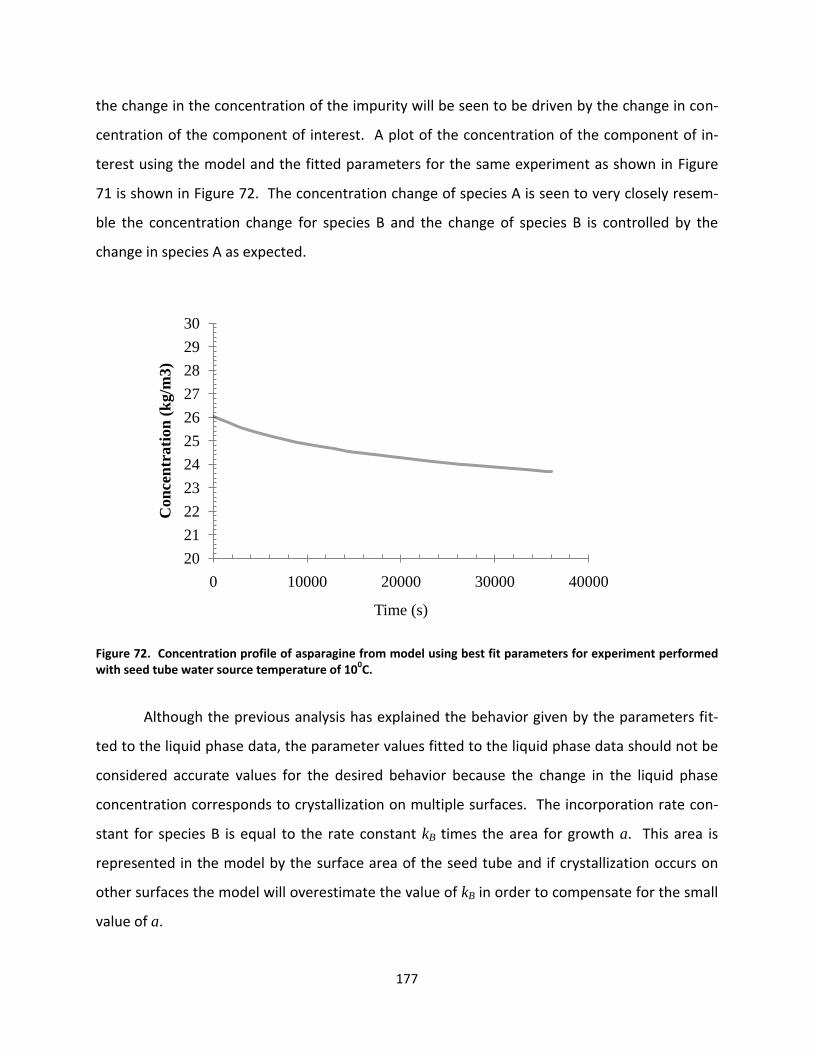
177

the change in the concentration of the impurity will be seen to be driven by the change in con-

centration of the component of interest. A plot of the concentration of the component of in-

terest using the model and the fitted parameters for the same experiment as shown in Figure

71 is shown in Figure 72. The concentration change of species A is seen to very closely resem-

ble the concentration change for species B and the change of species B is controlled by the

change in species A as expected.

Figure 72. Concentration profile of asparagine from model using best fit parameters for experiment performed with seed tube water source temperature of 100C.

Although the previous analysis has explained the behavior given by the parameters fit-

ted to the liquid phase data, the parameter values fitted to the liquid phase data should not be

considered accurate values for the desired behavior because the change in the liquid phase

concentration corresponds to crystallization on multiple surfaces. The incorporation rate con-

stant for species B is equal to the rate constant kB times the area for growth a. This area is

represented in the model by the surface area of the seed tube and if crystallization occurs on

other surfaces the model will overestimate the value of kB in order to compensate for the small

value of a.

20

21

22

23

24

25

26

27

28

29

30

0 10000 20000 30000 40000

Con

cen

trati

on

(k

g/m

3)

Time (s)

178

The plot of the SSR for the solid phase data shown in Figure 70 also has a valley at large

γ but there is now a distinct minimum point indicating a best fit set of parameter values. The

parameter values at this minimum are expected to provide a better representation of the sys-

tem and are considered the most representative values for describing asparagine and aspartic

acid in water.

4.3.2.4 Comparison of model predictions to the data using the fitted parameters

Predicted liquid phase concentration profiles for asparagine and aspartic acid using the

parameters fitted to the liquid and solid phase experimental data are shown in Figure 73 and

Figure 74 along with experimental data for an experiment performed with a seed tube water

source temperature of 50C. The solid phase data with predicted concentration profiles using

the best fit parameters from the liquid and solid phase data for the same experiment are pre-

sented in Figure 75. A plot of the solid phase data along with fitted curves using parameters

fitted to both liquid and solid phase data for an experiment performed with the seed tube wa-

ter source temperature at 150C is given in Figure 76.

The slight difference in the fit to the asparagine concentration in the liquid phase for the

two sets of parameters shown in Figure 73 occurs because the value of kA was the same for liq-

uid and solid phase fitting. Different values for γ and K affect the total amount of crystal grown

which affects the asparagine concentration in the batch model because the liquid-crystal inter-

face temperature depends on the total amount of crystal grown. The value of kA from the liq-

uid phase fit was used for solid phase analysis because the mole fraction of impurity (equation

(4.7)) has only a weak dependence on kA but a strong dependence on γ so that if kA is not fixed

a wide range of kA values can give the same fit.

These plots further indicate that the parameters fitted to the liquid phase concentration

profile are not representative of the modeled behavior. The presence of crystals on surfaces

other than the seed tube results in parameters fitted to the liquid phase data that are too large.

When these parameters are used to predict the impurity concentration profile in the solid

phase the predicted values are 2-10 times larger than the measured values as can be seen in

Figure 75 and Figure 76.

179

Figure 73. Concentration of asparagine versus time as determined by HPLC for a batch experiment with the seed tube water source at 50C and 2.6 g of asparagine and 0.4 g of aspartic acid in 100 g of water. The solid line is the curve representing the best fit of the batch crystallization model to the liquid phase data and the dashed line is the concentration profile predicted using the best fit parameters from the solid phase data for this experiment. The solution is stirred at 200 rpm and the water is passed through the seed tube at 1.4 LPM.

Figure 74. Concentration of aspartic acid versus time as determined by HPLC for a batch experiment with the seed tube water source at 50C and 2.6 g of asparagine and 0.4 g of aspartic acid in 100 g of water. The solid line is the curve representing the best fit of the batch crystallization model to the liquid phase data and the dashed line is the concentration profile predicted using the best fit parameters from the solid phase data for this expe-riment. The solution is stirred at 200 rpm and the water is passed through the seed tube at 1.4 LPM.

20

21

22

23

24

25

26

27

28

29

30

0 5000 10000 15000 20000 25000 30000 35000 40000

Con

cen

trati

on

asp

ara

gin

e (k

g/m

3)

Time (s)

Liquid Phase Data Fitted Parameters

Solid Phase Data Fitted Parameters

2.0

2.5

3.0

3.5

4.0

4.5

5.0

0 5000 10000 15000 20000 25000 30000 35000 40000

Con

cen

trati

on

asp

art

ic a

cid

(kg/m

3)

Time (s)



180

Figure 75. Mole fraction of aspartic acid versus relative crystal mass as determined by HPLC for a batch experi-ment with the seed tube water source at 50C and 2.6 g of asparagine and 0.4 g of aspartic acid in 100 g of water. The dashed line is the curve representing the best fit of surface mole fraction of impurity equation derived from the batch crystallization model to the data and the solid line is the prediction for the impurity mole fraction us-ing the parameters fitted to the liquid phase data. The solution is stirred at 200 rpm and the water is passed through the seed tube at 1.4 LPM.

Figure 76. Mole fraction of aspartic acid versus relative crystal mass as determined by HPLC for a batch experi-ment with the seed tube water source at 150C and 2.6 g of asparagine and 0.4 g of aspartic acid in 100 g of wa-ter. The dashed line is the curve representing the best fit of surface mole fraction of impurity equation derived from the batch crystallization model to the data and the solid line is the prediction for the impurity mole frac-tion using the parameters fitted to the liquid phase data. The solution is stirred at 200 rpm and the water is passed through the seed tube at 1.4 LPM.

0.00

0.05

0.10

0.15

0.20

0.25

0.30

0 0.2 0.4 0.6 0.8 1

Mole

Fra

ctio

n A

spart

ic A

cid


Liquid Phase Fitted Parameters

Solid Phase Fitted Parameters

0.00

0.10

0.20

0.30

0.40

0.50

0.60

0 0.2 0.4 0.6 0.8 1

Mole

Fra

ctio

n A

spart

ic A

cid




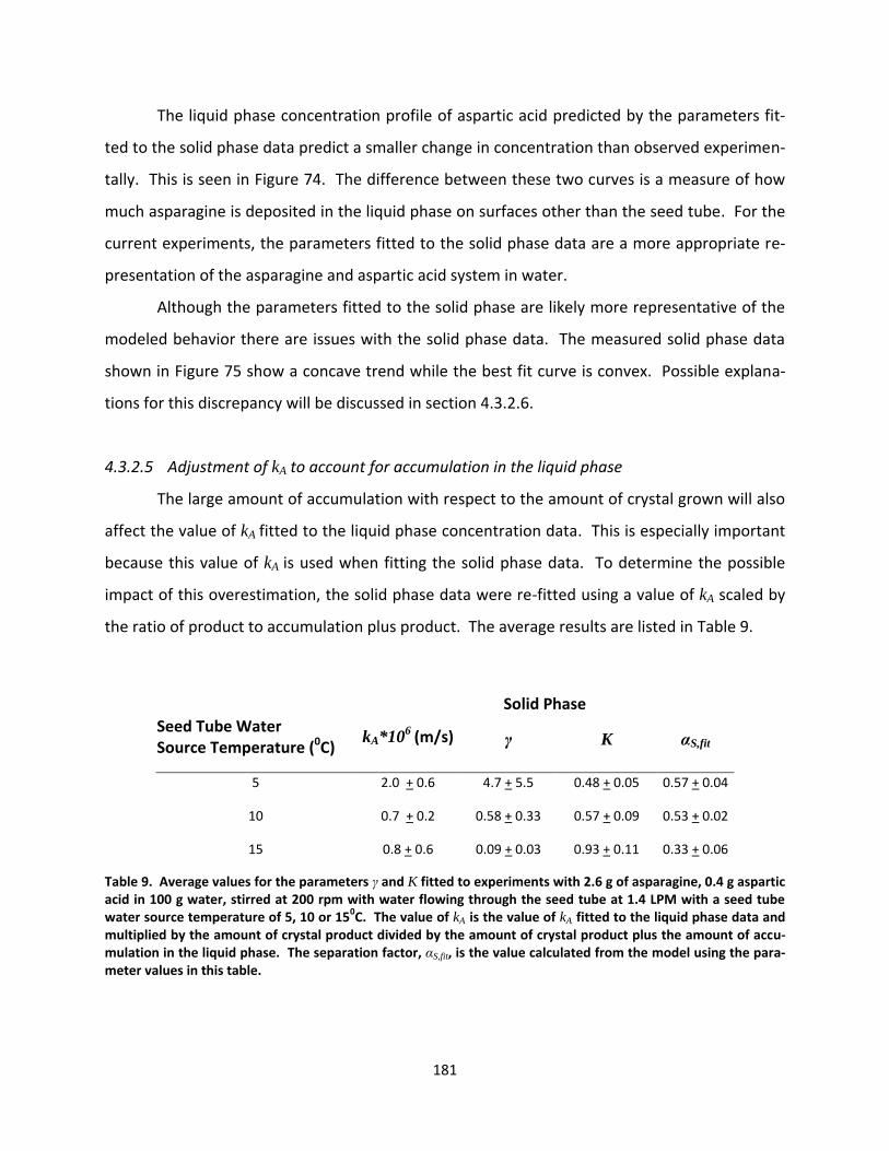
181

The liquid phase concentration profile of aspartic acid predicted by the parameters fit-

ted to the solid phase data predict a smaller change in concentration than observed experimen-

tally. This is seen in Figure 74. The difference between these two curves is a measure of how

much asparagine is deposited in the liquid phase on surfaces other than the seed tube. For the

current experiments, the parameters fitted to the solid phase data are a more appropriate re-

presentation of the asparagine and aspartic acid system in water.

Although the parameters fitted to the solid phase are likely more representative of the

modeled behavior there are issues with the solid phase data. The measured solid phase data

shown in Figure 75 show a concave trend while the best fit curve is convex. Possible explana-

tions for this discrepancy will be discussed in section 4.3.2.6.

4.3.2.5 Adjustment of kA to account for accumulation in the liquid phase

The large amount of accumulation with respect to the amount of crystal grown will also

affect the value of kA fitted to the liquid phase concentration data. This is especially important

because this value of kA is used when fitting the solid phase data. To determine the possible

impact of this overestimation, the solid phase data were re-fitted using a value of kA scaled by

the ratio of product to accumulation plus product. The average results are listed in Table 9.

Solid Phase

Seed Tube Water Source Temperature (0C)

kA*106 (m/s) γ K αS,fit

5 2.0 + 0.6 4.7 + 5.5 0.48 + 0.05 0.57 + 0.04

10 0.7 + 0.2 0.58 + 0.33 0.57 + 0.09 0.53 + 0.02

15 0.8 + 0.6 0.09 + 0.03 0.93 + 0.11 0.33 + 0.06

Table 9. Average values for the parameters γ and K fitted to experiments with 2.6 g of asparagine, 0.4 g aspartic acid in 100 g water, stirred at 200 rpm with water flowing through the seed tube at 1.4 LPM with a seed tube water source temperature of 5, 10 or 150C. The value of kA is the value of kA fitted to the liquid phase data and multiplied by the amount of crystal product divided by the amount of crystal product plus the amount of accu-mulation in the liquid phase. The separation factor, αS,fit, is the value calculated from the model using the para-meter values in this table.

182

The change in the parameters γ and K from Table 8 to Table 9 is small. The equivalent

parameter values show significant overlap between the two tables when considering the uncer-

tainties. This indicates that changing the value of kA has essentially no effect on the parameters

controlling impurity incorporation into the crystal. This is consistent with the expected beha-

vior based on analysis of the expression for the mole fraction of impurity in the crystal (equa-

tion (4.7)) and justifies use of the value of kA from liquid phase data fitting for solid phase data

fitting.

4.3.2.6 Discussion of surface impurity mole fraction trends from solid phase data

Although the parameters fitted to the solid phase data are more consistent with the ex-

perimental results, the fits to the solid phase data are qualitatively worse than the fits to the

liquid phase data. This occurs because of inconsistencies in the collected solid phase data. The

impurity concentration increases or stays constant as the total amount of crystal increases at

the beginning of the experiment but for experiments with cold water source at 5 and 100C the

aspartic acid concentration starts to decrease at some point during the experiment. The impur-

ity concentration in the solid for the experiments performed with a cold water source of 150C

continually increased during the entire growth process.

This two regime behavior is not expected to result from the fundamental growth

process because the concentrations of both species in the liquid phase decrease monotonically.

Additionally, the ratio of aspartic acid to asparagine in the liquid phase as characterized by the

solvent free mole fraction also decreases monotonically. With no inflection point in the liquid

phase data it is difficult to envision a mechanism by which the incorporation of impurity into

the solid phase undergoes the transition observed in the experimental data. It is possible that

the presence of crystallization on surfaces other than the seed tube is hiding any change in the

relative depletion of asparagine to aspartic acid caused by crystallization on the seed tube but

this cannot be determined from these experiments. Other factors involved with the experi-

mental setup or sampling procedure also must be explored as the cause of the observed beha-

vior.

183

The behavior of the solid data could be explained by errors in the solid phase analysis or

by a more complicated growth mechanism on the seed tube for the initial layers of crystal. Dur-

ing the sequential dissolution of the solid phase uniform dissolution was not observed for the

entire crystal mass. The initial dissolution operations maintained a qualitatively uniform crystal

layer on the seed tube but eventually some areas of the seed tube were dissolved more rapidly

than others leading to bare seed tube being exposed in some places. This often happened near

the top of the crystal. At this point, water is able to interact with the side of the crystal instead

of just the surface and dissolution can occur in two dimensions. This results in dissolution near

the top of the seed tube at a faster rate than over the total crystal mass. At this point subse-

quent dissolutions will contain material from different layers of the grown crystal and so the

impurity concentration measured will not correspond to the impurity concentration at the sur-

face.

If the total crystal had the same trend in impurity concentrations as the last few layers

of crystal grown, then the solid near the seed tube surface would have a higher impurity con-

centration and so would raise measured impurity concentration. Early dissolution of the higher

impurity concentration layers would serve to flatten the observed increase in impurity concen-

tration. This is consistent with some of the collected data where the measured impurity con-

centration is flat over the first portion of crystal growth before decreasing. This cannot explain

the data showing an initial increase in impurity concentration followed by a decrease in impuri-

ty concentration so dissolution from the top of the seed tube alone cannot account for all of

the trends observed in the solid impurity concentration results.

Variation in the growth of the first few layers of crystal could lead to the observed im-

purity concentration behavior. The seed tube is initially coated with polycrystalline pure aspa-

ragine. A pure asparagine seed may alter the crystallization behavior by favoring the incorpora-

tion of asparagine. The aspartic acid would be incorporated into the crystal gradually over the

first few layers before the full asparagine-aspartic acid solid solution is established. This is con-

sistent with an initial increase in impurity concentration that is observed in some experiments.

The initial variation in growth could also occur spatially. If different regions of the seed

tube grow at faster rates initially then the concentration in the initial layers of crystal would

184

represent an average from crystals grown at different time points. This disparity in initial

growth could result by inconsistent seeding on the surface of the seed tube but the crystal

would grow into a uniform surface over a period of time after which the impurity concentration

profile would be determined by the modeled behavior.

In the experiments conducted with the cold water source at 150C the monotonically in-

creasing impurity concentration could result from the initial growth behavior instead of funda-

mentally different parameter values. The amount of crystal growth in these experiments is very

small and there may not be enough crystal grown to overcome the initial growth process and to

establish a uniform surface for further growth.

It is also possible that there is a transition between high and low γ behavior between a

source water temperature of 5 and 150C. The predicted behavior with γ>1 is decreasing impuri-

ty concentration with growth and with γ<1 is increasing impurity concentration. A change in

the value of γ with respect to one seems unlikely because the temperature at the surface varies

with crystal growth and there is a large amount of overlap in the range of temperature expe-

rienced at the crystal surface. Any issues leading to the non-monotonic nature of the collected

solid phase data must also be addressed before addressing this possibility.

The discussion in this section has given possible explanations for the observed behavior

in the solid phase data but the major finding is that further experimental work is necessary.

Experiments that generate larger amounts of crystal and experimental techniques that give

more consistent sampling of the grown crystal are needed for comparison to model predictions.

The parameter values fitted to the collected solid phase data in these experiments were found

to give reasonable average results through comparison of the separation factor but further

work is necessary for comparing model predictions to the impurity concentration profile in the

crystal.

4.3.2.7 Discussion of dissolution rate

The dissolution experiments performed on pure asparagine indicate that mass transfer

to the surface is not the rate limiting step in the crystal growth process. This conclusion as-

sumes that the dissolution rate is a reasonable approximation to the mass transfer rate. This is

185

supported by the estimation of the mass transfer coefficient using the Chilton-Colburn analogy

in section 4.2.4. The estimated value of the mass transfer coefficient in that section was

2.3*10-5 m/s which compares favorably to the value of (2.4+0.4)*10-5 m/s determined by para-

meter fitting to data obtained from dissolution experiments at 250C

The dissolution rate determined from experiment is 10-50 times larger than any of the

fitted values for the incorporation rate constant of asparagine. The most appropriate values of

kA to use for comparison are those for experiments with seed tube water source temperature

at 150C because this temperature range is the closest to the conditions at which the dissolution

rate was measured.

The estimated values of kA for those experiments were 0.3*10-5 m/s directly from fitting

of the liquid phase concentration and 0.04*10-5 m/s if the fitted parameter is scaled by the ratio

of product to product plus accumulation. The most appropriate comparison point is the smaller

value because of the previously discussed overestimation of parameters from the liquid phase

concentration data. This smaller value is nearly two orders of magnitude less than the meas-

ured dissolution rate and would be expected to be even smaller if the temperature of the seed

tube water source was moved closer to 250C. This indicates that the growth of crystal on the

seed tube is not diffusion limited. Surface incorporation kinetics are the rate determining step.

4.3.2.8 Summary of Experimental Discussion

Due to the presence of solid in the bulk liquid the parameters fitted to the solid phase

data are the most appropriate for describing the crystallization behavior of asparagine and as-

partic acid in water. The parameters fitted to the solid phase data do a better job of explaining

the overall impurity distribution in the solid and separation factor between the solid and liquid

phases when an appreciable amount of solid is grown but the solid phase data does not allow

clear interpretation.

Larger amounts of crystal growth and improved solid sampling methods are important

in order to generate clearer data from the solid phase analysis to determine the value of γ in

relation to one and determine the appropriate trend in the surface mole fraction of impurity.

Further experiments that severely limit the amount of crystallization on surfaces other than the

186

seed tube or at least give much larger ratios of growth on the seed tube to growth on other sur-

faces in the liquid phase are needed so that the accurate parameters can be found from liquid

phase concentration data.

4.4 Summary of Experimental Work

Batch experiments with asparagine as the component of interest and aspartic acid as

the impurity have been conducted in order to provide data to validate the model proposed in

Chapter 2. The model system for experimentation was asparagine and aspartic acid in water

which forms a solid solution with up to 15% aspartic acid in the asparagine crystal lattice. The

crystal growth surface is a piece of aluminum tubing coated with asparagine and with water

flowing through the interior to provide temperature control. The growth of crystal in this sys-

tem provides a significant thermal resistance which results in a changing temperature at the

solid-liquid interface. The model for the batch experiment was modified to account for the

changing temperature at the solid-liquid interface.

The parameters fitted to the solid phase data were found to be more representative of

the experimental results than the parameters fitted to the liquid phase data. This is due to the

presence of crystals in the liquid phase on surfaces other than the seed tube which affect the

parameter values fitted to liquid phase concentration measurements. The presence of crystals

in the bulk also results in overprediction of kA but this was not found to have an effect on the

parameters fitted to the solid phase data. This indicates that the value of kA does not have a

strong effect on the fitting of the solid phase data collected in these experiments.

The measurement of the solid phase concentration profile by sequential dissolution was

not perfect. The concentration profile showed non-monotonic behavior which may result from

uneven dissolution of the sample or from a different mechanism for the initial crystal growth on

the seed tube. Uneven dissolution was observed but cannot entirely account for the observed

behavior so a combination of these two mechanisms or other factors seems likely.

The parameters fitted to the solid phase were able to more closely match the measured

concentration profiles and separation factor than the liquid phase fitted parameters even with

this uncertainty. Due to the experimental method, these parameters represent an average val-

187

ue over the range of temperature experienced at the solid-liquid interface. The magnitude of

these values is instructive but the absolute values as a function of temperature cannot be de-

termined.

The experimental method described here provides evidence that the proposed model

can reasonably describe crystallization of a solid solution but it is far from conclusive. Avoiding

crystals in the bulk solution was not possible in these experiments but should be improved

upon for future experimentation. Additionally, the solid phase analysis was not as reliable as

the liquid phase analysis and further adaptation of the analysis method should be explored in

order to get more reliable data.

The experiments have been shown to be very reproducible in terms of crystal yield. One

possibility for improved solid phase analysis is to perform a series of experiments with the same

initial conditions but different end times. The total solid could then be dissolved and a differen-

tial analysis of the solid behavior could be performed with the results from multiple experi-

ments. This would eliminate issues related to product sampling.

189

5. Conclusions

5.1 Summary of Findings

A staged, semi-continuous, counter current crystallization process has been proposed

that seeks to constrain crystal growth to solid surfaces in order to avoid multi-phase fluid han-

dling while allowing for multiple recrystallizations to provide improved purity but comparable

yield to batch crystallization. Processes that avoid multi-phase flow handling problems and that

can be run in a continuous manner would be beneficial for integration into new continuous

processing schemes.

A model for crystallization of solid solutions was proposed and applied to batch crystalli-

zation and the new process. The proposed model was tested against batch crystallization expe-

riments. The new process was proposed with the goal of providing increased purity compared

to batch crystallization with yield approaching that of batch crystallization run until completion.

The yield is constrained by the solubility of the component of interest in the system solvent and

therefore batch crystallization run until completion will give the maximum yield at a specified

temperature.

Analysis shows that the proposed crystallization model is capable of predicting concen-

tration gradients in the solid phase. This is an important characteristic of a model seeking to

describe crystallization of solid solutions on surfaces because the amount of impurity incorpo-

rated into the crystal will vary with concentration for a solid solution. This has been demon-

strated for crystallization of solid solutions in melt crystallization.113

The impurity incorporation behavior is controlled by two model parameters, γ and K.

These parameters are characteristic of the particular chemical system in use and must be

measured experimentally. The ratio of the incorporation rate constants of the impurity to the

component of interest is γ and K is an equilibrium constant describing the relationship between

the concentrations at the solid surface and the equilibrium concentrations in the bulk. These

parameters are expected to depend on temperature but not concentration.

Variation of these model specific parameters resulted in determination of parameter

regimes in which the proposed crystallization process can provide better performance than

190

batch crystallization. The proposed process with the solid removed as the product was found

to be advantageous when γ<1 and K less than order 1 with smaller values of K providing better

results.

When γ>1 and K is close to or greater than one the process can also deliver a favorable

result if the liquid effluent is taken as the product and the solid output is discarded as waste.

This situation results in a high yield, high purity liquid product ready for the next processing op-

eration but these parameter values are not expected to happen for a large number of systems.

Additional operating variables such as the sweep stream flow rate and the number of

stages were also explored. It was found that a sweep stream offers an increase in purity at the

cost of a significant decrease in yield indicating that the use of a sweep stream is not desirable.

Increasing the number of stages was shown to be favorable and resulted in higher purities at

yields close to the maximum yield. The benefit of increasing the number of stages diminishes

as more and more stages are added and the cost of construction and operation of a large cas-

cade should also be considered when designing the process.

The proposed process provides the best results when the liquid from the last tank is dis-

carded at the end of every growth stage. Any tank used during the process will provide a larger

benefit as an active tank for crystal growth than as a vessel to facilitate liquid transfer which

means that the use of a liquid handling tank is not favorable and the process should be operat-

ed with removal of the liquid from the last tank at the end of each growth stage.

Experiments conducted with asparagine as the component of interest and aspartic acid

as the impurity in water in order to test the validity of the model encountered some difficulties.

The seed tube used as the designated growth surface does not present a constant temperature

at the crystallization surface because the growing crystal layer will resist heat transfer and the

temperature at the liquid-solid interface will increase with time. The fitted parameters

represent an average over the temperature profile observed at the liquid-solid interface. An

experimental design that allows for constant temperature at the solid-liquid interface would

simplify data analysis and provide more valuable information. This could potentially be

achieved by varying the flow rate or temperature of the coolant in the seed tube flow loop.

191

Constraint of crystal growth is an important principle of the new process but is difficult

to achieve in practice. The batch experiments that were performed were unable to eliminate

crystallization on surfaces other than the seed tube and this resulted in significant depletion

from the liquid phase due to undesired crystallization. The model fitted to the liquid phase

concentration data did not generate reasonable values for the model parameters because of

this undesired crystallization.

The amount of crystallization occurring on undesired surfaces could be limited by de-

creasing the overall supersaturation or increasing the bulk temperature. Decreasing the super-

saturation would also result in smaller amount of product on the desired surface but this option

could be pursued by using a large number of tanks with a small amount of supersaturation in

each tank. This could be accomplished by implementing a decreasing temperature profile along

the length of the cascade.

If the bulk temperature is raised in relation to the temperature at the surface for crystal-

lization the amount of undesired crystallization should decrease. Raising the bulk temperature

will raise the solubility in the bulk so that crystal will be less likely to be present on a non-cooled

surface.

Fitting the model to the experimental solid phase data indicate that the value of K was

roughly 0.5-1 for experiments with a temperature range of 5-250C. The value of γ was found to

be less than one for experiments conducted with seed tube water source temperatures 10 and

150C but greater than one with a large standard deviation for a seed tube water source tem-

perature of 50C. The fitted parameter values for experiments performed with a seed tube wa-

ter source temperature of 10 and 150C are in the range where the proposed process is pre-

dicted to give favorable results with the crystal being removed as the product.

The point of these experiments was not to determine if asparagine and aspartic acid

could be separated by the proposed process but instead to determine if the proposed model

was able to describe a real system. Batch experiments indicate that the proposed model is rea-

sonably consistent with the collected data but inconsistencies in the experimental data make

this conclusion uncertain.

192

The collected solid phase data were somewhat ambiguous resulting in uncertainty as to

the fitted parameter values. For most of the experiments an initial increase was followed by a

decrease in the mole fraction of impurity across the growing crystal. This change in behavior is

unexpected because the liquid phase data indicates a monotonic change in concentration and

liquid phase mole fraction. Model fitting resulted in best fit curves that were in some cases

convex while the data itself was concave. The presence of undesired crystallization in the liquid

phase may be masking a change in the liquid phase concentrations capable of explaining the

observed solid phase behavior but this cannot be learned from the current experiments and

issues with the solid phase growth process and data collection seem more likely culprits.

The observed behavior for the solid phase concentration profile could be explained by

any uneven growth during the initial crystallization and/or complications with the solid phase

analysis procedure. The initial growth may not be uniform over the entire surface. If islands of

material grow at different rates initially before eventually joining together the sampling method

would then remove samples from different time points which would change the measured con-

centrations. After an initial period the islands join together and then are constrained to grow in

one direction which gives the final macroscopically uniform product. The initial seed layer was

pure asparagine and this may impact the initial growth of crystal. The incorporation of aspartic

acid into the crystal may change as the crystal changes from pure asparagine into a solid solu-

tion of asparagine and aspartic acid.

Growing thicker layers of crystal would help to address both of these issues by minimiz-

ing the uncertain layers of growth with respect to the total amount of growth. Thicker layers of

crystal could be grown by decreasing the initial temperature at the seed tube surface or by de-

creasing the diameter of the seed tube. Other experimental designs with different seed surfac-

es may also be useful in circumventing this problem.

The solid phase analysis also resulted in uneven dissolution of crystal after a certain

amount of crystal was dissolved. The initial dissolutions give qualitatively even dissolution but

eventually the crystal at the top of the seed tube is totally removed and the bare seed tube is

exposed. At this point dissolution continues from exterior face of the crystal but also from the

edge exposed by total dissolution at the top of the seed tube. This impact of this problem could

193

be minimized by increasing the thickness of the collected crystal so that the effect dissolutions

represent only a small fraction of the total crystal grown.

As an alternative analysis method to the sequential dissolution of the solid phase, mul-

tiple experiments could be performed with identical conditions but different end times. The

total concentration of the crystals grown in these experiments could then be measured and a

differential analysis could be used to find the concentration profile in the crystal. The amount

of crystal growth was found to be reproducible in these experiments indicating that a differen-

tial analysis may be possible.

Further experiments are necessary to determine if the proposed model is capable of de-

scribing crystallization on solid surfaces for a solid solution forming system. These experiments

need to further minimize crystallization on surfaces other than the seed tube to make fitting of

parameters to the liquid phase concentrations useful and increase the total amount and thick-

ness of product so that more consistent solid data can be collected.

5.2 Future Work

Validation of the proposed model by experiment should be the focus of any future work.

In order to do this, experiments must be designed that provide even growth on a defined sur-

face while minimizing any other growth in the system. Minimizing growth in undesired loca-

tions could possibly be done by increasing the bulk temperature of the liquid so that particles

are less likely to exist on non-cooled surfaces or by changing the stirring rate or stir bar type to

minimize contact nucleation and particle attrition from the seed tube.

Finding a new way to promote growth on a specific surface may also be advantageous.

Designed surfaces for nucleation of a specific chemical would simplify processing and might

promote growth on the desired surface in relation to growth on other surfaces in the vessel.

Alternative shapes for the seed tube could also be studied. A flat plate would be more

appropriate for use with the model as implemented in this work and this becomes more impor-

tant as the thickness of the crystal layer increases. The challenge of using a flat plate is to de-

sign the heat transfer such that the temperature across the plate could be held at a constant

value.

194

If the proposed model is found to be appropriate then the effect of varying the temper-

ature profile along the cascade should be explored. A temperature profile will allow control

over the degree of supersaturation in each tank which will be important for minimizing homo-

geneous nucleation and may also provide some benefit to the product purity. A temperature

profile will result in a larger number of stages being needed to achieve high yields but the mag-

nitude of this difference can be estimated by simulation.

If the proposed model is found to not be appropriate then a new model for crystalliza-

tion should be proposed and used to study the semi-continuous process. The same procedure

outlined in this document can be followed with a different model to determine whether the

proposed process has benefits compared to batch crystallization.

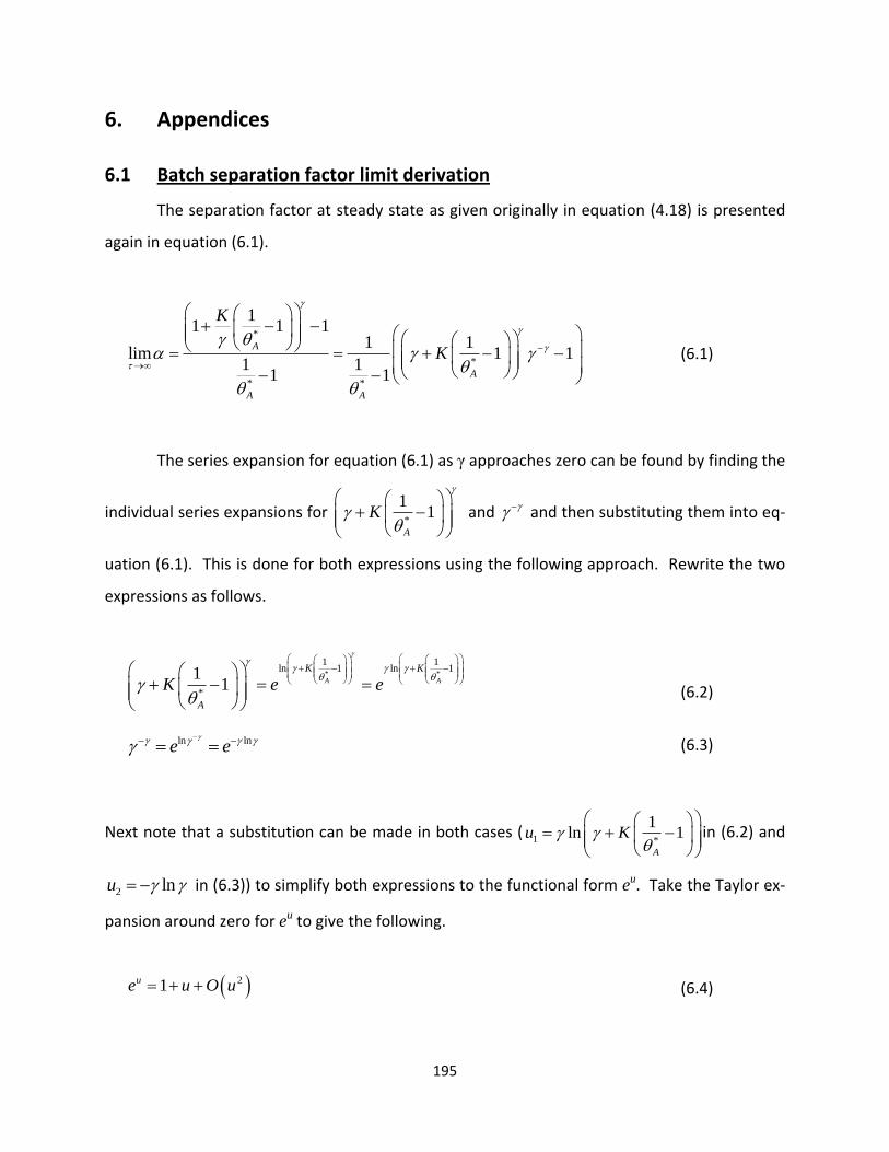
195

6. Appendices

6.1 Batch separation factor limit derivation

The separation factor at steady state as given originally in equation (4.18) is presented

again in equation (6.1).

*

*

* *

11 1 1

1 1lim 1 1

1 11 1

A

A

A A

K

K

(6.1)

The series expansion for equation (6.1) as γ approaches zero can be found by finding the

individual series expansions for *

11

A

K

and and then substituting them into eq-

uation (6.1). This is done for both expressions using the following approach. Rewrite the two

expressions as follows.

* *

1 1ln 1 ln 1

*

11 A A

K K

A

K e e

(6.2)

ln lne e

(6.3)

Next note that a substitution can be made in both cases (1 *

1ln 1

A

u K

in (6.2) and

2 lnu in (6.3)) to simplify both expressions to the functional form eu. Take the Taylor ex-

pansion around zero for eu to give the following.

21ue u O u (6.4)

196

To finish, insert the appropriate u for each of the two expressions into equation (6.4).

2

* *

1 11 1 ln 1

A A

K K O

(6.5)

21 ln lnO (6.6)

197

6.2 Analytical Yield for Counter-Current Crystallization Process

The following derivation is for a three stage cascade with the feed entering at stage two

and sweep stream entering at stage one. The volume of liquid in each tank is assumed to be

constant (dilute solution), the temperature is the same and constant in every tank, the order of

the supersaturation dependence is one and the surface area of crystal growth is constant (1-

dimensional plane growth). The dimensionless variables are defined as in section 2.3.1. This

analysis will only deal with species A so all θ values will omit the subscript A. θi will indicate the

concentration of species A in tank i. Because the temperature is assumed constant the satura-

tion concentration and incorporation rate constants in all tanks are equal and will be

represented by θ* and β. Additionally the liquid transfer considerations dealing with over and

under filled tanks will not be taken into account during this derivation.

The differential equation describing tank one is presented in equation (6.7).

*10 1 1

d

d

(6.7)

The Laplace transform of equation (6.7) is taken and this equation can be solved and inverted

to give the concentration profile as a function of time for tank one. This is shown in equations

through (6.8)-(6.10).

*

0 01 1 1s

(6.8)

*0

011

s s s

(6.9)

*

0 01 1 1f e e

(6.10)

The following substitutions will be used to simplify notation during this derivation.

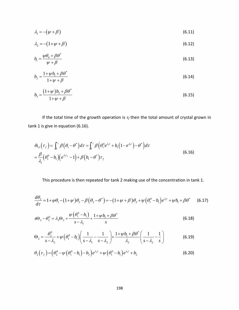
198

1 (6.11)

2 1 (6.12)

*

01b

(6.13)

*

12

1

1

bb

(6.14)

*

2

3

1

1

bb

(6.15)

If the total time of the growth operation is τf then the total amount of crystal grown in

tank 1 is give in equation (6.16).

1 1

1

* 0 *

1 1 1 10 0

0 *

1 1 1

1

1

1

f f

f

c f

f

m d e b e d

b e b

(6.16)

This procedure is then repeated for tank 2 making use of the concentration in tank 1.

1* 0 *21 2 2 2 1 1 11 1 1

db e b

d

(6.17)

0 *1 10 1

2 2 2 2

1

1b bs

s s

(6.18)

0 *

02 12 1 1

2 1 2 2 2

11 1 1 1bb

s s s s s

(6.19)

2 10 0 0

2 2 1 1 2 1 1 2f b b e b e b (6.20)

199

2 1

*

2 20

0 0 0 *

2 1 1 2 1 1 2

2 1

1 1

f

f f

c f

f

m d

b b e b e b

(6.21)

The concentration in tank 3 can then be found making use of the concentrations in tanks

1 and 2.

2 1

*32 3 3

0 0 0 *

3 2 1 1 2 1 1 2

1 1

1 1

d

d

b b e b e b

(6.22)

0 0 02 1 1 2 1 10

3 3 2 3

2 1

*

2

1 1

1

b b bs

s s

b

s

(6.23)

0 0 002 1 1 2 1 13

3 2

2 1 22

*

2

2

1 1

1

b b b

s s ss

b

s s

(6.24)

2 2

1

0 0 0 0

3 3 1 1 3 2 1 1 2

0

1 1 3

1 1

1

f b b e b b e

b e b

(6.25)

200

2

2

2

1

*

3 30

0 0

3 1 1 3

2

0 0

2 1 1 2

2 2

0 *

1 1 3

1

1 1

11

1

f

f

f

f

f

c f

f

f

m d

b b e

eb b e

b e b

(6.26)

The initial conditions for the next growth cycle are determined by the final concentra-

tions during the previous growth cycle. This relationship for each of the three tanks is detailed

below where the subscript j will indicate a particular growth cycle.

0

1, 1, 1 2, 1j j f c j fm (6.27)

0

2, 2, 1 3, 1j j f c j fm (6.28)

0

3, 3, 1j j f (6.29)

The condition of cyclic steady state occurs when 0 0

, , 1i j i j . When this is the case, equations

(6.27)-(6.29) can be solved to give explicit expressions for 0

i . This is done starting with tank 3

and working backwards. The algebra involved in generating the expressions for 0

i is substan-

tial and will be omitted in this derivation.

2 2

1

0 0 0 0 0

3 3 1 1 3 2 1 1 2

0

1 1 3

1 1

1

b b e b b e

b e b

(6.30)

201

2

2

2

1

0

1 1 3

0 0 0

3 2 1 1 2

0

1 1 3

1

11

1

1

f

f

f

f

f

b b e

b b ee

b e b

(6.31)

2 1

2

2

2

1

0 0 0 0

2 2 1 1 2 1 1 2

0 0

3 1 1 3

2

0 0

2 1 1 2

2 2

0 *

1 1 3

1

1 1

11

1

f

f

f

f

f

f

b b e b e b

b b e

eb b e

b e b

(6.32)

2 2

1

2 1

0

1 1 2 2

2

0

1 1 20

2

0

2 1 1

2 1 2

*

3

1 1

1

1 1 1 1 1

f f

f

f f

f

b b e e

b e b

e b e

b

(6.33)

2

1

0 0

1 1 1 1

0 0

2 1 1 2

2

0 *

1 1 2

1

1

1

f

f

f

f

b e b

b b e

b e b

(6.34)

202

1

1

21 2

1 2

*

3* 2

2 2 2

20

1

2

2

1 2

1 11

1

1 11

f

f

f

f

b e

bb

e

(6.35)

The yield from this process at cyclic steady state is given by the expression in equation

(6.36).

1c

f

my

(6.36)

The expressions for 0

i can be used to find the final expression for 1cm .

1

1

1

21 2

1 2

*

3* 2

2 2 2

2 *

1 1 1

12

2

1 2

*

3* 2

2 2 2

2*

1

1

1 11

11

1 11

f

f

f

f

f

c f f

f

f

f

b e

bb

m b e b

e

bb

b

2

2

1 2

*

1

*

2

1 2

2

2

*

3

2 1 2

22 2

1

11

1

1

1

f

f

f

b

b

b

(6.37)

203

*

1

*

2

1 2

2

2

*

3

2 1 2

22 2

1

1

1

y b

b

b

(6.38)

Replacing all of the substituting variables with their definitions gives equation (6.39) which is

the result presented in section 2.3.2.

**0

**0

*

2

**0

*

*

2

1

1

1

1 1

1

11

1

11 1

1 1 1

y

(6.39)

If the sweep stream flow rate is set equal to zero in equation (6.39) the result is equal to

the yield from a two stream cascade with feed at stage 1 and no sweep stream. This result is

shown in equation (6.40).

204

**

*

**

* *

2

2*

2

1

1

11

1 1 1

1

1 11 1 1

11

11

y

(6.40)

The maximum possible yield at steady state from a single tank would be *11

.

Because β is strictly greater than one it is evident that multiple tanks employing this cyclical

process result in a higher maximum attainable yield.

205

6.3 Analytical Concentration Profile for Species B When γ<<1 or γ>>1 and

K<<1

The following derivations are for a one stage cascade with the feed entering and sweep

stream entering at stage one. Solutions to equations can be done using the same methods as

outlined in appendix 6.2. A one stage system is not expected to employ a sweep stream in

practice but it is used for this derivation in order to provide a simpler final expression for the

purity. The expression giving the product purity is

1

1

Ac

BcAc B BcB

Ac

mp

mm m

m

(6.41)

where all values are at cyclical steady state. The volume of liquid in each tank is assumed to be

constant (dilute solution), the temperature is the same and constant in every tank, the order of

the supersaturation dependence is one and the surface area of crystal growth is constant (1-

dimensional plane growth). The dimensionless variables are defined as in section 2.3.1. The

liquid transfer considerations dealing with over and under filled tanks are not needed for a one

stage system.

The general solution to the impurity concentration profile cannot be determined analyt-

ically. The model defined in section 2.3 defines the equilibrium concentration of the impurity

species in terms of the time dependent concentrations of species A and B. This leads to a diffe-

rential equation that cannot be solved. In order to generate analytical solutions, two special

cases were considered.

The first case is γ<<1. In this situation the incorporation rate constant of the impurity

into the crystal is much smaller than the incorporation of the component of interest so only a

small amount of B will be included in the crystal. In this case the equilibrium concentration of

species B in the liquid phase will be nearly constant at the initial value. Assuming that the equi-

librium concentration of B in the liquid phase is constant allows for the model to be solved ana-

lytically.

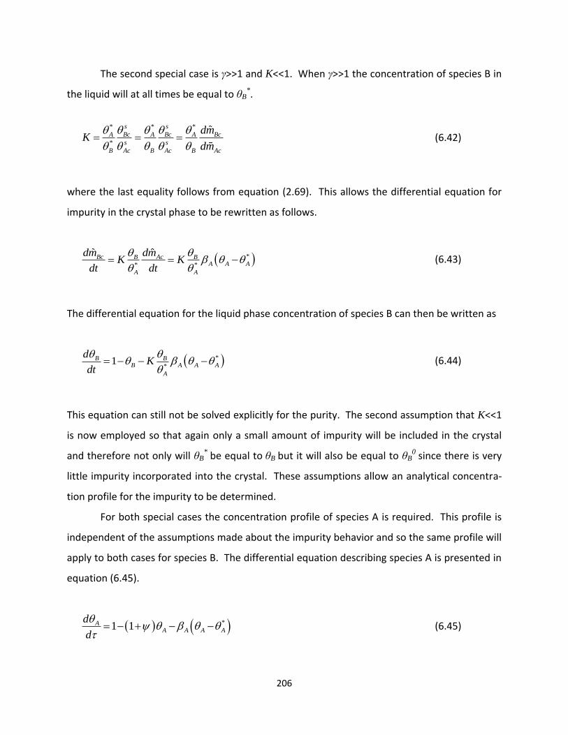
206

The second special case is γ>>1 and K<<1. When γ>>1 the concentration of species B in

the liquid will at all times be equal to θB*.

* * *

*

s s

Bc Bc BcA A A

s s

B Ac B Ac B Ac

dmK

dm

(6.42)

where the last equality follows from equation (2.69). This allows the differential equation for

impurity in the crystal phase to be rewritten as follows.

*

* *

Bc AcB BA A A

A A

dm dmK K

dt dt

(6.43)

The differential equation for the liquid phase concentration of species B can then be written as

*

*1B B

B A A A

A

dK

dt

(6.44)

This equation can still not be solved explicitly for the purity. The second assumption that K<<1

is now employed so that again only a small amount of impurity will be included in the crystal

and therefore not only will θB* be equal to

θB but it will also be equal to θB

0 since there is very

little impurity incorporated into the crystal. These assumptions allow an analytical concentra-

tion profile for the impurity to be determined.

For both special cases the concentration profile of species A is required. This profile is

independent of the assumptions made about the impurity behavior and so the same profile will

apply to both cases for species B. The differential equation describing species A is presented in

equation (6.45).

*1 1AA A A A

d

d

(6.45)

207

The solution to this equation with the concentration of species A at time zero equal to θA0 is

*

1 10 11

1A

A AA

A

e e

(6.46)

At cyclical steady state the following relation will be true.

0

A A f (6.47)

This expression is very simple because in the one stage system the solid contents are removed

after every growth stage as the product. This derivation can be extended to multiple tank sys-

tems but the resulting profiles are complicated and difficult to analyze.

Equation (6.47) can then be solved to give the concentration profile of species A during

a growth stage when cyclic steady state has been achieved.

* * *

1 11 1 11

1 1 1

A A A A A AA

A A A

e e

(6.48)

The concentration of species A in the liquid phase is seen to be constant at all times when cyc-

lical steady state is achieved in a one stage system. This answer makes sense because the liquid

is not changed between successive growth stages so that the conditions at the end of one

growth stage are identical to those at the beginning of the next.

The amount of species A in the solid phase is also necessary and is given by the follow-

ing equation.

*

* 1 1

1

AAcA A A A

A

dm

dt

(6.49)

208

*

0 * 1 1

1

AAc A A A A

A

m

(6.50)

6.3.1 Impurity concentration profile when γ<<1

The differential equation for the impurity in this case is given by

*1 1BB B B B

d

d

(6.51)

When θB* is constant as it is in this case that this is the exact same functional form as for species

A. The solutions for species A can then be used directly when the subscript A is replaced with a

subscript B.

*

1 10 11

1

B BB B

B

e e

(6.52)

Determination of the initial concentration at cyclical steady state is slightly complicated be-

cause θB* depends on the value of θB

0. This dependence is given by

0

*

0 *

*1

B

A

B

A

A

K

(6.53)

The value of θB0 is then found to be

0

*

0 *

1

11

1

A

B

B

A

AK

(6.54)

209

Substituting this expression into equation (6.52) gives the impurity profile at cyclical steady

state.

*

0 *

1

11

1

A

B

B

A

AK

(6.55)

As in the case of species A, the concentration of species B at cyclical steady state is constant.

The amount of species B in the crystal phase is then found as

* 0

0 *

*

0

* *

*0 * 0 *

0 *

*

0 *

11

1

1 1 1

111 1

1

1

1 1

A

A A

A

A

BcB B B B B

A

A

B B B

A AB

AA A

A

B

AB

A

dm

Kdt

K K

K

K

(6.56)

*

0 *

1

1 1

A

Bc B

AB

A

m

K

(6.57)

The purity is given by

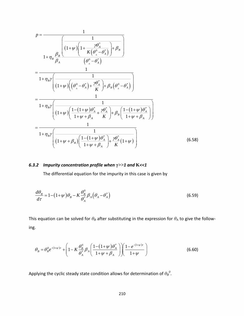
210

*

0 *

0 *

*0 * 0 *

* **

*

1

1

1 1

1

1

11

1

1

11

1 1 1 11

1 1

1

11

1 11

1

A

A

A A

AB

AB

B

A A

B

AA B A

B

A AAB

A A

B

AB

p

K

K

K

*

1A

A K

(6.58)

6.3.2 Impurity concentration profile when γ>>1 and K<<1

The differential equation for the impurity in this case is given by

0

*

*1 1B B

B A A A

A

dK

d

(6.59)

This equation can be solved for θB after substituting in the expression for θA to give the follow-

ing.

* 1010

*

1 1 11

1 1

ABB B A

A A

ee K

(6.60)

Applying the cyclic steady state condition allows for determination of θB0.

211

0

*

*

1

1 11

1

B

AA

A A

K

(6.61)

When this is substituted into equation (6.60) the concentration profile for the impurity at cyc-

lical steady can be determined and it is found again to be constant at the initial value.

0

B B (6.62)

The determination of the purity in this case is slightly simpler than in the previous case because

the explicit expression for the amount of impurity in the solid phase does not need to be calcu-

lated. Equation (6.43) allows this quantity to be determined in relation to the amount of spe-

cies A in the solid phase with the initial condition that there is no solid present.

0

*

BBc Ac

A

m K m

(6.63)

The purity can then be written as follows.

0

** *

*

1

1

1 1

111

1 11

1

Ac

BcAc B BcB

Ac

BBB

AA AA

A A

mp

mm m

m

KK

K

(6.64)

213

6.4 Analytical Concentration Profile for Species B in Tank 1 When γ=1

For a system with N stages, feed at stage 1, no sweep stream, dilute concentrations, and

short times an analytical expression for the concentration of the impurity in tank 1 can be de-

termined for an arbitrary growth cycle. The value at cyclic steady state cannot be determined

though so the solution will contain the initial concentrations at the beginning of the growth

cycle, θA0 and θB

0. The differential equations governing the concentration profile of species A

and B in tank 1 are given in equations (6.65) and (6.66).

*11 11A

A A A A

d

d

(6.65)

*11 11B

B B B B

d

d

(6.66)

Equation (6.65) can be solved readily to give the concentration profile of species A in tank 1.

1

* *10

1

1 1

1 1A

A

A A A AA

A A

e

(6.67)

The critical concentration of the impurity, θB*, is given by the following expression as shown in

section 2.2.2.

1

*

* ** 10

**

1 11 11 1

A

A

B BB

A A AA A

AA A A

K Ke

(6.68)

Substituting equation (6.68) into equation (6.66) and rearranging gives

214

1

11* *

10

*

1 11 1

11 1

A

A

B BB B

A A A

A A A

d

d Ke

(6.69)

This equation is a first order differential equation and can be solved using an integrating factor.

To find the integrating factor the following integral must be evaluated

1

1

1

* *10

*

* *10

*

*10

* *

11 1

11 1

11 1

11 1

11

1 1

1

A

A

A

A

A

A

BB

A A A

A A A

BB

A A A

A A A

B B

A A A

A A A

dK

e

dK

e

K Ke

1

1

*

1

* *10

* *

* *0

* **

*

11

11 1

11 1

1 1 11 ln

1 111

1

A

A

A

A

A

B B

A A A

A A A A

B

A A A AB

A A AA

A A

d

ed

K Ke

K K

K

11 A

A

e

(6.70)

The integrating factor is then given by

1

* *10

* **

*

1 1 1exp 1 ln 1

1 111

1

A

A

B

A A A AB

A A A AA

A A

K Ke

K

215

*

*

1

* * 11 11 10

1* *

1 11

1 1

B

AAB A

AAA

KA A A

A A A A

K Ke e

(6.71)

The concentration profile for species B in tank 1 is given by

1B

d C

(6.72)

where C is the constant of integration. Evaluating the integral of μ will be simpler to follow

with use of the following constants.

*0

1*

1

1

A AA

A A

KB

(6.73)

*

*

11

1

A

A A

KD

(6.74)

The integral to be evaluated is

1 1 1

B

B A A De B De d

(6.75)

This equation cannot be evaluated analytically unless βB is equal to βA, or γ=1. If all values of βB

are set equal to βA, equation (6.75) can be evaluated to give

11 1

1 1 1

1 11

A

A A A

A A A

CD

AA

A

B Dee B De d

DD

(6.76)

Substituting into equation (6.72) gives the concentration profile for B in terms of the in-

tegration constant.

216

11 1

1

1 1 1

1 11

A

A A

A

A A A

C

AA

A

B

C

B DeC

DD

e B De

(6.77)

The concentration at τ=0 is θB10. Using this to evaluate the integration constant C gives

the final result.

1 11 01 11

1

1

1 1 1

1 11 01 11

1

1 1

1 1 1 11 1

1 11

AA

A AA

A

A

A

A A A

AA

A AA

A

A

A

A A

C CB

A ACA A

A A

B

C

C CB

A CA

A

B De B D

B CD DD D

e B De

B De B D

B CDD

e B De

1 A C

(6.78)

Now rewrite equation (6.68) as

217

1

1

* 1 11 1* *

10

*

1 11 01 11

1

11 1

1

11 1

1 11

1 1

1 11

1

A

A

A

A

AA

A AA

A

A

A

A A

A

A A

B BB

A A A

A A A

D DB

A DA

A

D

D

e

B DeKe

B De B D

B DDD

B De

B D

B De

1

110 1

1

1

11

1 101 1 11

11 1

0

1

11 1

1

1

1

1 1

1 1

A

A

A

A A

A

A

A

A

A A

A A A

A

A A

A

A A

D

DB

A A D

D

D DB

A A D

B

A A A A

B De

DB D

B D

B DB De

D B DB De

B D

D B D DB De

1

1

A

A D

D

(6.79)

The following equations will simplify the final result

*

*

* *

11 1 1 1 1

1

AA A A A A

A A A

K KD

(6.80)

* *

0 0 *

1 1* * *

1 11 1

1 1

A A AA A A

A A A A A

K K KB D

(6.81)

**

**

*

*

*

*

1 1 11 1 1 11 1

1

1 1

1 1

A A A

A AA AA

AA A

A

A

A A

A

KD K

K

K

(6.82)

218

The expression for θB1* can now be written as

*

*

*

*

0* 11

* 0 * *

1* * *

1 1

1 10 *

1*

* *10

1* *

1 1*

1 1 1 1 1

1

1 11

1 1

A

A

A A

A

A

BB

A A A A

A A A

K

K

A A

A

A A AA

A A A A

K K K

K

K Ke

(6.83)

This is the result presented in equation (2.93).

219

6.5 Solid Solution Verification

Asparagine and aspartic acid have been found in the literature to form a solid solution

containing up to 20% aspartic acid in asparagine.148, 149 In order to validate this, supersaturated

solutions at five different concentrations were prepared. The compositions of these solutions

are listed in Table 10.

Asparagine (g) Aspartic Acid (g) Water (g) xASN *103 xASP *103

3 0.5 100 4.07 0.68

3.1 0.4 100 4.20 0.54

3.2 0.3 100 4.34 0.41

3.3 0.2 100 4.48 0.27

3.4 0.1 100 4.61 0.14

Table 10. Composition of solutions prepared in order to check for solid solution formation by asparagine and aspartic acid in water. xi is the mole fraction of species i.

The asparagine, aspartic acid and water were heated to 800C until the solids had com-

pletely dissolved. The mixtures were then allowed to cool to room temperature at which point

a liquid sample was taken for HPLC analysis. The solutions were then stirred for 5 days at room

temperature. Crystals were observed in the first four solutions after 24 hrs and the fifth solu-

tion contained crystals after 48 hrs. Stirring is continued for 5 days to allow equilibrium to be

approached in both the liquid and solid phase.

Once the 5 days had elapsed, each solution was filtered and the solid and liquid phases

were collected. A sample was prepared from the liquid and solid phases for HPLC analysis. The

liquid phase samples were prepared in the same manner as samples from batch crystallization

experiments (section 4.2.1). The solid phase was prepared for HPLC analysis by dissolving ap-

proximately 70 mg of solid in 100 ml of water. The concentrations of asparagine and aspartic

acid in the prepared samples were then measured with HPLC.

The phase behavior will be shown using a standard 2-dimensional plot with the mole

fraction of asparagine on the x-axis and the mole fraction of aspartic acid on the y-axis. The

220

mole fraction of water can be found by subtracting the sum of these two mole fractions from

one. The crystal grown is a mono-hydrate so the highest possible mole fraction of asparagine in

the solid phase is 0.5 corresponding to a pure asparagine crystal. A plot of the phase behavior

showing primarily the solid phase compositions is given in Figure 77. The liquid phase concen-

trations are too small to be seen on the same plot as the solid phase concentrations so they will

be addressed in a different figure.

Figure 77. Partial phase diagram for asparagine and aspartic acid in water.

It is clear in Figure 77 that the solid phase compositions for the five test solutions are all

different. This is the expected result as a eutectic or compound forming system would a con-

stant solid composition.

Figure 78 shows the initial and liquid phase concentrations.

0.000

0.005

0.010

0.015

0.020

0.025

0.030

0 0.1 0.2 0.3 0.4 0.5

Asp

Mole

Fra

ctio

n

Asn Mole Fraction

3.0 g asn 0.5 g asp

3.1 g asn 0.4 g asp

3.2 g asn 0.3 g asp

3.3 g asn 0.2 g asp

3.4 g asn 0.1 g asp

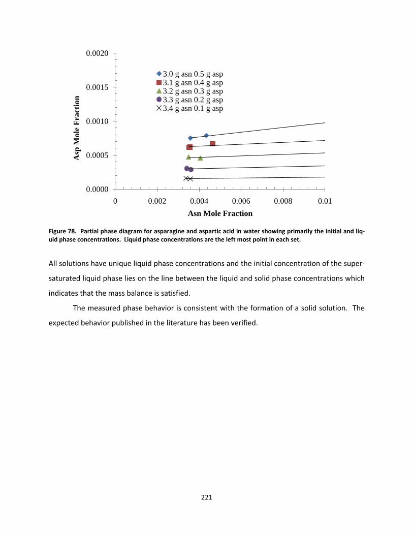
221

Figure 78. Partial phase diagram for asparagine and aspartic acid in water showing primarily the initial and liq-uid phase concentrations. Liquid phase concentrations are the left most point in each set.

All solutions have unique liquid phase concentrations and the initial concentration of the super-

saturated liquid phase lies on the line between the liquid and solid phase concentrations which

indicates that the mass balance is satisfied.

The measured phase behavior is consistent with the formation of a solid solution. The

expected behavior published in the literature has been verified.

0.0000

0.0005

0.0010

0.0015

0.0020

0 0.002 0.004 0.006 0.008 0.01

Asp

Mole

Fra

ctio

n

Asn Mole Fraction

3.0 g asn 0.5 g asp3.1 g asn 0.4 g asp3.2 g asn 0.3 g asp3.3 g asn 0.2 g asp3.4 g asn 0.1 g asp

223

7. References

1. W. H. Power, B. M. Fabuss and C. N. Satterfield, Journal of Chemical & Engineering Data 9 (3), 437-442 (1964).

2. V. Costodes and A. Lewis, Chem. Eng. Sci. 61 (5), 1377-1385 (2006).

3. I. D. G. A. Putrawan and T. H. Soerawidjaja, Separation and Purification Technology 39, 79-88 (2004).

4. L. F. Filobelo, O. Galkin and P. G. Vekilov, The Journal of Chemical Physics 123 (1), 014904-014901 - 014904-014907 (2005).

5. A. Che and C. Rey, Journal of Materials Science: Materials in Medicine 10, 231-237 (1999).

6. D. G. Georgieva, M. E. Kuil, T. H. Oosterkamp, H. W. Zandbergen and J. P. Abrahams, Acta Crystallographica Section D Biological Crystallography 63 (5), 564-570 (2007).

7. M. Järn, S. Areva, V. Pore, J. Peltonen and M. Lindén, Langmuir 22, 8209-8213 (2006).

8. X. Y. Liu, Langmuir 16, 7337-7345 (2000).

9. X. Y. Liu, Journal of Physical Chemistry B 105, 11550-11558 (2001).

10. T. E. Paxton, A. Sambanis and R. W. Rousseau, Langmuir 17, 3076-3079 (2001).

11. R. P. Sear, Physical Review E 67 (6) (2003).

12. N. E. Chayen, E. Saridakis and R. P. Sear, Proceedings of the National Academy of Sciences 103 (3), 597-601 (2005).

13. V. F. Komarov, J. Garside and J. W. Mullin, Chem. Ind. (3), 119-120 (1976).

14. M. L. White and A. A. Frost, Journal of Colloid Science 14 (3), 247-251 (1959).

15. J. L. Kenty and J. P. Hirth, Surface Science 15 (3), 403-& (1969).

16. J. Aizenberg, Nature 1720 (1971), 1997-2000 (1999).

17. K. Fujiwara, S. Nagahisa, J. Yano, S. Ueno and K. Sato, Journal of Physical Chemistry B, 8116-8123 (2000).

18. T. Kubo, Journal of Crystal Growth 269 (2-4), 535-541 (2004).

19. E. M. Landau, S., M. Levanon, L. Leiserowitz, M. Lahav and J. Sagiv, Journal of the American Chemical Society 111, 1436-1445 (1989).

20. D. Palms, C. Priest, R. Sedev, J. Ralston and G. Wegner, Journal of Colloid and Interface Science 303 (2), 333-336 (2006).

224

21. H. Takiguchi, K. Iida, S. Ueno, J. Yano and K. Sato, Journal of Crystal Growth 193, 641-647 (1998).

22. A. M. Travaille, E. G. A. Steijven, H. Meekes and H. Kempen, Journal of Physical Chemistry B 109, 5618-5626 (2005).

23. P. W. Carter and M. D. Ward, Journal of the American Chemical Society 115, 11521-11535 (1993).

24. P. W. Carter and M. D. Ward, Journal of the American Chemical Society (116), 769-770 (1994).

25. N. B. J. Hetherington, A. N. Kulak, K. Sheard and F. C. Meldrum, Langmuir 22 (5), 1955-1958 (2006).

26. A. McPherson and P. Shlichta, Science 239 (4838), 385-387 (1988).

27. N. A. Clontz and W. L. McCabe, Chemical Engineering Progress Symposium Series, No. 110 67, 6-17 (1971).

28. R. T. Johnson, R. W. Rousseau and W. L. McCabe, AICHE Symposium Series No. 121 68, 31-41 (1972).

29. J. W. Mullin and S. J. Jancic, Transactions of the Institution of Chemical Engineers 57 (3), 188-193 (1979).

30. A. H. Janse and E. J. Dejong, Transactions of the Institution of Chemical Engineers 56 (3), 187-193 (1978).

31. M. Volmer, Kinetik der phasenbildung. (T. Steinkopff, Dresden und Leipzig, 1939).

32. D. Kashchiev and G. M. van Rosmalen, Crystal Research and Technology 38 (78), 555-574 (2003).

33. D. Knezic, J. Zaccaro and A. S. Myerson, Journal of Physical Chemistry B 108 (30), 10672-10677 (2004).

34. O. Sohnel and J. W. Mullin, Journal of Colloid and Interface Science 123 (1), 43-50 (1988).

35. J. W. Gibbs, The collected works of J. Willard Gibbs. (Yale Univ. Press, New Haven, 1948).

36. R. Becker and W. Döring, Annalen der Physik 416 (8), 719-752 (1935).

37. M. Avrami, Journal of Chemical Physics 7, 1103-1112 (1939).

38. W. A. Johnson and R. F. Mehl, TRANSACTIONS OF THE AMERICAN INSTITUTE OF MINING AND METALLURGICAL ENGINEERS 135, 416-442 (1939).

39. A. N. Kolmogorov, IZV AKAD NAUK SSSR Ser Math 1, 355-359 (1937).

40. M. Castro, Physical Review B 67 (3), 1-8 (2003).

225

41. P. Chaing, M. D. Donohue and J. L. Katz, Journal of Colloid and Interface Science 122 (1), 251-265 (1988).

42. M. Iwamatsu, The Journal of Chemical Physics 126 (13), 134703-134703 (2007).

43. X. Y. Liu, Journal of Chemical Physics 111 (4), 1628-1635 (1999).

44. R. Mohanty, S. Bhandarkar and J. Estrin, AIChE Journal 36 (10), 1536-1544 (1990).

45. P. C. Rieke, 182, 472-484 (1997).

46. J. W. P. Schmelzer, Materials Physics and Mechanics 6, 21-33 (2003).

47. R. M. Tromp and J. B. Hannon, Surface Review and Letters 9 (3 & 4), 1565-1593 (2002).

48. W. Wu and G. H. Nancollas, Journal of Colloid and Interface Science 182, 365-373 (1996).

49. Y. Kousaka, T. Nomura and M. Alonso, Advanced Powder Technology 12 (3), 291-309 (2001).

50. A. D. J. Haymet and D. W. Oxtoby, The Journal of Chemical Physics 74 (4), 2559-2565 (1981).

51. T. V. Ramakrishnan and M. Yussouff, Physical Review B 19 (5), 2775 (1979).

52. S. M. Kathmann, Theoretical Chemistry Accounts 116 (1-3), 169-182 (2006).

53. L. A. Baez and P. Clancy, The Journal of Chemical Physics 102 (20), 8138-8148 (1995).

54. Y. G. Chushak and L. S. Bartell, The Journal of Physical Chemistry B 103 (50), 11196-11204 (1999).

55. Y. Chushak and L. S. Bartell, The Journal of Physical Chemistry A 104 (41), 9328-9336 (2000).

56. J. Anwar and P. K. Boateng, Journal of the American Chemical Society 104 (15), 9600-9604 (1998).

57. D. Frenkel and J. P. McTague, Annual Review of Physical Chemistry 31 (1), 491-521 (1980).

58. E. S. Boek, W. J. Briels and D. Feil, The Journal of Physical Chemistry 98 (6), 1674-1681 (1994).

59. P. Chiang and M. D. Donohue, Journal of Colloid and Interface Science 122 (1), 230-250 (1988).

60. A. A. Chernov, (1989), pp. 391-417.

61. W. K. Burton, N. Cabrera and F. C. Frank, Philosophical Transactions of the Royal Society A: Mathematical, Physical and Engineering Sciences 243 (866), 299-358 (1951).

62. A. A. Chernov, Soviet Physics Uspekhi 4 (1), 116-148 (1961).

63. G. H. Gilmer, R. Ghez and N. Cabrera, Journal of Crystal Growth 8 (1), 79-93 (1971).

226

64. A. Berthoud, Journal de Chimique Physique 10, 624-635 (1912).

65. J. J. P. Valeton, Zeitschrift fur Kristallographie 59, 483 (1924).

66. J. W. Mullin, Crystallization. (Elsevier Butterworth-Heinemann, Boston, 2001).

67. J. Garside, Chem. Eng. Sci. 40 (1), 3-26 (1985).

68. K. A. Jackson, in Liquid metals and solidification; a seminar on liquid metals and solidification held during the thirty-ninth National Metal Congress and Exposition, Chicago, November 2 to 8, 1957, edited by M. American Society for (Cleveland, 1958), pp. 174-186.

69. P. Bennema and J. P. van der Eerden, Journal of Crystal Growth 42, 201-213 (1977).

70. J. R. Bourne and R. J. Davey, Journal of Crystal Growth 36 (2), 278-286 (1976).

71. S. Briarqon, D. Colson and J. P. Klein, Chemical Engineering Journal 70, 55-64 (1998).

72. T. R. Bott, Experimental Thermal and Fluid Science 14, 356-360 (1997).

73. P. Martins and F. Rocha, Chem. Eng. Sci. 61 (17), 5686-5695 (2006).

74. G. H. Montillon and W. L. Badger, Industrial & Engineering Chemistry 19 (7), 809-816 (1927).

75. W. L. McCabe, Industrial & Engineering Chemistry 21 (1), 30-33 (1929).

76. W. L. McCabe, Industrial & Engineering Chemistry 21 (2), 112-119 (1929).

77. A. D. Randolph and M. A. Larson, AIChE Journal 8 (5), 639-645 (1962).

78. J. Garside and R. J. Davey, Chem. Eng. Commun. 4 (4-5), 393-424 (1980).

79. M. Bavin, Chem. Ind. (16), 527-529 (1989).

80. A. Asmadi, M. A. Neumann, J. Kendrick, P. Girard, M.-A. Perrin and F. J. J. Leusen, The Journal of Physical Chemistry B 113 (51), 16303-16313 (2009).

81. B. B. Averkiev, M. Y. Antipin, A. B. Sheremetev and T. V. Timofeeva, Crystal Growth & Design 5 (2), 631-641 (2004).

82. A. R. Browning, M. F. Doherty and G. H. Fredrickson, Physical Review E 77 (4), 041604 (2008).

83. R. J. Davey and J. W. Mullin, Kristall und Technik 11 (3), 229-233 (1976).

84. R. J. Davey, Journal of Crystal Growth 34, 109-119 (1976).

85. A. S. Michaels and A. R. Colville, The Journal of Physical Chemistry 64 (1), 13-19 (1960).

86. J. W. Mullin and Amataviv.A, Journal of Applied Chemistry of the Ussr 17 (5), 151-& (1967).

227

87. N. Kubota and J. W. Mullin, Journal of Crystal Growth 152 (3), 203-208 (1995).

88. R. J. Davey and J. W. Mullin, Journal of Crystal Growth 26 (1), 45-51 (1974).

89. S. Al-Jibbouri and J. Ulrich, Crystal Research and Technology 39 (6), 540-547 (2004).

90. K. G. Denbigh and E. T. White, Chem. Eng. Sci. 21 (9), 739-& (1966).

91. A. S. Myerson and M. Saska, Aiche Journal 30 (5), 865-867 (1984).

92. K. Sato, Japanese Journal of Applied Physics 19 (7), 1257-1266 (1980).

93. K. Sato, Japanese Journal of Applied Physics 19 (10), 1829-1836 (1980).

94. A. S. Dzyuba, Soviet Physics Crystallography 28 (1), 111-112 (1983).

95. A. S. Myerson and D. J. Kirwan, Industrial & Engineering Chemistry Fundamentals 16 (4), 414-420 (1977).

96. N. Clavaguera, V. Palumbo-Romand, M. Ferriol and M. T. Cohen-Adad, Growth (Lakeland) 180, 248-254 (1997).

97. Q. Nie, J. Wang and Q. Yin, Chem. Eng. Sci. 61 (18), 5962-5968 (2006).

98. G. G. Z. Zhang and D. J. W. Grant, International Journal of Pharmaceutics 181, 61-70 (1999).

99. L. Bonpunt, R. Courchinoux, Y. Haget, E. Estop, T. Calvet, M. a. Cuevas-Diarte and M. Labrador, Journal of Applied Crystallography 24 (2), 164-170 (1991).

100. A.-L. Chow, P. K. K. Chow, W. Zhongshan and D. J. W. Grant, International Journal of Pharmaceutics 24, 239-258 (1985).

101. A. S. Teja, J. C. Givand and R. W. Rousseau, AIChE Journal 48 (11), 2629-2634 (2002).

102. R. M. Myasnikova, Molecular Crystals and Liquid Crystals 90 (1), 195-204 (1983).

103. G. T. Didrikhsons and H. Pfeiffer, PHYSICA STATUS SOLIDI A-APPLIED RESEARCH 169, 169-178 (1982).

104. A. G. Shtukenberg, Y. O. Punin and P. Azimov, American Journal of Science 306, 553-574 (2006).

105. H. A. Doerner and W. H. Hoskins, Journal of the American Chemical Society 47 (3), 662-675 (1925).

106. R. Meadhra and R. Lin, Chemical Engineering Research and Design 84 (8), 711-720 (2006).

107. J. C. Givand, A. S. Teja and R. W. Rousseau, AIChE Journal 47 (12), 2705-2712 (2001).

108. J. Givand, B.-K. Chang, A. S. Teja and R. W. Rousseau, Industrial & Engineering Chemistry Research 41 (7), 1873-1876 (2002).

228

109. F. Rosenberger and H. G. Riveros, The Journal of Chemical Physics 60 (2), 668-673 (1974).

110. J. A. Burton, R. C. Prim and W. P. Slichter, The Journal of Chemical Physics 21 (11), 1987-1991 (1953).

111. P. A. Meenan, S. R. Anderson and D. L. Klug, in Handbook of industrial crystallization, edited by A. S. Myerson (Butterworth-Heinemann, Boston, 1993).

112. B. R. Thomas, A. A. Chernov, P. G. Vekilov and D. C. Carter, Journal of Crystal Growth 211 (1-4), 149-156 (2000).

113. G. J. Sloan and A. R. McGhie, Techniques of Melt Crystallization. (Wiley-Interscience, New York, 1988).

114. M. Oullion, F. Puel, G. Fevotte, S. Righini and P. Carvin, Chem. Eng. Sci. 62 (3), 820-832 (2007).

115. F. Ricard, C. Brechtelsbauer, X. Y. Xu and C. J. Lawrence, Chemical Engineering Research and Design 83 (7), 794-805 (2005).

116. A. G. Jones and J. W. Mullin, Chem. Eng. Sci. 29 (1), 105-118 (1974).

117. J. W. Mullin and J. Nyvlt, Chem. Eng. Sci. 26 (3), 369-& (1971).

118. K. Hanaki, N. Nonoyama, Y. Yabuki, Y. Kato and I. Hirasawa, Journal of Chemical Engineering of Japan 40 (1), 63-71 (2007).

119. M. A. Novomeysky, Transactions of the Institution of Chemical Engineers 14, 60-84 (1936).

120. J. L. Manganaro and J. C. Schwartz, Industrial & Engineering Chemistry Process Design and Development 24 (4), 1245-1251 (1985).

121. F. Jeremiassen and H. Svanoe, Chemical and Metallurgical Engineering 39, 594-596 (1932).

122. I. GEA Process Engineering, in http://www.niroinc.com/evaporators_crystallizers/Oslo_type_crystallizer.asp, edited by Oslo_type_crystallizer_fg4.jpg (2010).

123. H. H. Newman and R. C. Bennett, Chemical Engineering Progress 55 (3), 65-70 (1959).

124. R. Castelnuovo, in http://en.wikipedia.org/wiki/File:DTB_2.PNG (2006).

125. J. N. Robinson and J. E. Roberts, Canadian Journal of Chemical Engineering 35, 105-112 (1957).

126. J. S. Wey and J. P. Terwilliger, Industrial & Engineering Chemistry Process Design and Development 15 (3), 467-469 (1976).

127. H. S. Weng, Journal of Chemical Engineering of Japan 13 (5), 407-409 (1980).

128. A. E. Bailey, Melting and solidification of fats. (Interscience Publishers, New York, 1950).

http://www.niroinc.com/evaporators_crystallizers/Oslo_type_crystallizer.asp

http://en.wikipedia.org/wiki/File:DTB_2.PNG

229

129. A. E. Bailey, D. Swern, M. W. Formo and T. H. Applewhite, Bailey's Industrial oil and fat products. (Wiley, New York, 1979).

130. W. KLOEK, T. VAN VLIET and P. WALSTRA, Journal of Texture Studies 36 (5-6), 544-568 (2005).

131. L. Chen, J. Li and M. Matsuoka, Industrial and Engineering Chemistry Research 45, 2818-2823 (2006).

132. M. A. van der Gun, O. S. L. Bruinsma and G. M. van Rosmalen, Chem. Eng. Sci. 56 (7), 2381-2388 (2001).

133. G. G. Devyatykh, Y. E. Elliev, Y. P. Kirillov and A. Y. Malyshev, Inorg. Mater. 36 (10), 1050-1055 (2000).

134. H. Schildknecht, Zone melting. (Verlag Chemie;Academic Press, Weinheim/Bergstr.,New York, 1966).

135. J. A. Brodie, Mechanical and Chemical Engineering Transactions 7 (1), 37-44 (1971).

136. O. Fischer, S. J. Jancic and K. Saxer, in Industrial Crystallization 84 (9th Symposium, The Hague), edited by S. J. Jancic and E. J. de Jong (Elsevier, Amsterdam, 1984), pp. 153-157.

137. K.-J. Kim and A. Mersmann, Chemical Engineering Research and Design 75 (2), 176-182 (1997).

138. J. Sobesto and J. Mydlarz, Chemische Technik 43 (6), 227-230 (1991).

139. J. W. Mullin and J. R. Williams, Chemical Engineering Research & Design 62 (5), 296-302 (1984).

140. K. Bartosch and A. Mersmann, Chem. Eng. Sci. 56 (7), 2347-2356 (2001).

141. E. W. Merrow, Chemical Engineering Progress 81 (5), 14-22 (1985).

142. E. W. Merrow, Chemical Engineering 95 (15), 89-92 (1988).

143. D. Schulze, Powders and bulk solids : behavior, characterization, storage and flow. (Springer, Berlin; New York, 2007).

144. W. L. Godfrey and R. D. Benham, Simulation 4 (1), 27-33 (1965).

145. W. L. Godfrey, (1969).

146. J. P. Roodenrijs and W. H. J. M., (1988).

147. A. Poulos, J. W. Greiner and G. A. Fevig, Industrial and Engineering Chemistry 53 (12), 949-962 (1961).

148. D. M. Ruthven and C. B. Ching, Chem. Eng. Sci. 44 (5), 1011-1038 (1989).

149. J. B. Dalton and C. L. A. Schmidt, Journal of Biological Chemistry 109, 241-248 (1935).

230

150. CRC handbook of chemistry and physics. (1978).

151. Netzsch, Operating and Maintenance Instructions for Mini-Metering Pumps. (1999).

152. F. W. Dittus and L. M. K. Boelter, International Communications in Heat and Mass Transfer 12 (1), 3-22.

153. L. Addadi, Z. Berkovitch-Yellin, N. Domb, E. Gati, M. Lahave and L. Leiserowitz, Nature 296 (4), 21-26 (1982).

154. J. L. Wang, Z. Berkovitch-Yellin and L. Leiserowitz, Acta Crystallographica Section B Structural Science 41 (5), 341-348 (1985).

155. C. A. Zittle and C. L. A. Schmidt, Journal of Chemical Biology 108, 161-185 (1934).

156. T. H. Chilton and A. P. Colburn, Industrial and Engineering Chemistry 26, 1183-1187 (1934).

157. A. P. Colburn, Transactions of the American Institute of Chemical Engineers 29, 174-210 (1933).

158. W. Hayduk and H. Laudie, AIChE Journal 20 (3), 611-615 (1974).

159. J. R. Partington, An advanced treatise on physical chemistry, Vol. 1 Fundamental Principles: the Properties of Gases. (Longmans, Green, London; New York, 1949).

160. Y. Ma, C. Zhu, P. Ma and K. T. Yu, Journal of Chemical & Engineering Data 50 (4), 1192-1196 (2005).

161. R. C. Dorresteijn, L. G. Berwald, G. Zomer, C. D. de Gooijer, G. Wieten and E. C. Beuvery, Journal of Chromatography A 724 (1-2), 159-167 (1996).

162. J. W. J. Henderson and A. Brooks, (Agilent Technologies 5990-4547EN, 2010).

a process for separation by semi-continuous counter

Documents