a process model of rho gtp-binding proteins in the context of phagocytosis

A Process Model of Rho GTP-bindingProteins in the Context of Phagocytosis

Luca Cardelli 1,2

Microsoft Research7 JJ Thomson Avenue, CB3 0FB, Cambridge, UK

Philippa Gardner 3

Department of ComputingImperial College, London, UK

Ozan Kahramanogulları 4

Department of Computing &Centre for Integrative Systems Biology

Imperial College, London, UK

Abstract

At the early stages of the phagocytic signalling, Rho GTP-binding proteins play a key role. With thestimulus from the cell membrane and with the help from the regulators (GEF, GAP, Effector, GDI), theseproteins serve as switches that interact with their environment in a complex manner. We present a genericprocess model for the Rho GTP-binding proteins, and compare it with a previous model that uses ordinarydifferential equations. We then extend the basic model to include the behaviour of the GDIs. We discussthe challenges this extension brings and directions of further research.

Keywords: phagocytosis, GTP-binding proteins, stochastic π-calculus, process modeling

1 We would like to thank Andrew Phillips for discussions on the SPiM language, Emmanuelle Caron for hercomments and suggestions which helped to shape Section 4, and Jaroslav Stark for proof reading the paperand also suggesting improvements in the presentation. Cardelli acknowledges support of a visiting profes-sorship at Imperial College. Gardner acknowledges support of a Royal Academy of Engineering/MicrosoftResearch Cambridge Senior Fellowship. Kahramanogulları acknowledges support of the UK Biotechnologyand Biological Sciences Research Council through the Centre for Integrative Systems Biology at ImperialCollege (grant BB/C519670/1).2 Email: [email protected] Email: [email protected] Email: [email protected]

Electronic Notes in Theoretical Computer Science 194 (2008) 87–102

1571-0661/$ – see front matter © 2008 Elsevier B.V. All rights reserved.

www.elsevier.com/locate/entcs

doi:10.1016/j.entcs.2007.12.007

mailto:[email protected]



http://www.elsevier.com/locate/entcs

1 Introduction

Phagocytosis is a form of endocytosis by which a cell engulfs micro-organisms,large edible particles and cellular debris. Phagocytosis literally means ‘cell eating’.Single-celled organisms such as amoeba obtain food in this way. Phagocytosis alsooccurs in multi-celled organisms when, for example, macrophages and other whiteblood cells defend the body against invasions of harmful viruses, bacteria, cancerousbody cells, and other threats to health [1]. A key project in the newly-formedCentre for Integrative Systems Biology at Imperial is to analyse the fundamentalmechanisms for phagocytosis, using the expertise of biologists, computer scientistsand mathematicians. Our part of the project is to use stochastic process algebras,such as the stochastic π-calculus (see, e.g., [18]), to provide a compositional andscalable notation for simulating phagocytosis.

In this first paper, we give a process calculus model of Rho GTP-binding pro-teins which play an important role also in phagocytosis. These proteins act on themembranes of cells as molecular switches in several subcellular activities, regulatinga variety of cell functions such as actin organisation, cell shape and cell adhesion.We study Goryachev and Pokhilko’s paper [11] on an ordinary differential equation(ODE) analysis of the Rho GTP-binding protein cycle, first in isolation and thenwith their regulators GEF and GAP. Our process models provide a simple, compo-sitional description of the Rho GTP-binding protein cycle, where the structure ofmodels naturally follows the structure of the biological models. Using the StochasticPi Machine (SPiM) [17,16] and the rates of interaction described in [11], we providesimulations which precisely mimic the results given using ODEs. Following [11], wealso extend our model to include the effectors which interact with these proteinsat the membrane. Again, our results remain consistent with the results obtainedfrom the ODE analysis. Our results provide an essential starting point for ourinvestigation of the behaviour of Rho GTP-binding proteins using process models.

We further extend our model to include the interactions of the GTP-bindingproteins with another class of regulators called GDIs, which were not incuded inthe ODE analysis of [11]. Our initial aim was to analyse two biological modelsdescribed in the survey paper [7]. Instead, based on discussions with Caron, a biol-ogist at Imperial, we introduce a hybrid model which fits more closely with currentknowledge. We extend our process model, again illustrating the compositional na-ture of our approach. The next step is to provide a systematic study of the rates,searching the biological literature and using SPiM to explore the parameter spaceleading to sensible behaviour. We begin this study, using SPiM to explore the effectof varying the quantity of the GDI protein on the behaviour of the protein cycleand the effectors. Ultimately, we require help from the biologists to fill the gapsin our current knowledge. Indeed, our ambitious goal is to create a research en-vironment where the biological experiments corroborate and provide data for ourprocess-model simulations, and our simulations guide the biological experiments.

L. Cardelli et al. / Electronic Notes in Theoretical Computer Science 194 (2008) 87–10288

2 Rho GTP-binding Proteins and their Role in FcReceptor-mediated Phagocytosis

Phagocytosis is the process whereby cells engulf large particles, usually over 0.5μm

in diameter, by a mechanism that is based on local rearrangement of the cytoskele-ton. Phagocytosis plays an essential role in host defence against invading pathogens,and in clearance of cell corpses generated by programmed cell death or apoptosis.Phagocytosis contributes to inflammation and the immune response [1].

Phagocytosis is a triggered process, often initiated by the interaction of particle-bound ligands (opsonins) with specific receptors on the cell membrane of ‘profes-sional’ phagocytic white blood cells such as macrophages, neutrophils and dendriticcells [5]. Among the variety of surface proteins dedicated to phagocytosis, Fc recep-tors (FcRs) and receptors for complement fragments (Cr’s) mediate the clearenceof pathogens covered by the specific antibody or complement respectively [12].

2.1 Fc Receptor-mediated Phagocytosis

In the context of Fc receptor-mediated phagocytosis, the signalling cascade is trig-gered by antibodies, called immunoglobulin, e.g., IgG, which protect the organismby binding to the surface of infectious microorganisms to form a coat. In this sit-uation, the tail region of each antibody molecule, called the Fc region, is exposedon the exterior. This antibody coat is recognised by specific Fc receptors on thesurface of the cell. Their binding induces the phagocytic cell to extend pseudopodsand extend its tips to form a phagosome while proceeding with binding its ligandsin a zipper like fashion around the internalised particle [10].

As a result of FcR-Fc interaction on the exterior surface of the cell membrane,a protein tyrosine kinase of the Src family is activated. Following this, Src phos-phorylates two tyrosine residues on the receptor’s signalling subunits located on theinternal tail of the Fc receptor. These tyrosine residues belong to immunorecep-tor tyrosine-based activation motifs, or ITAMs. Another protein tyrosine kinase,Syk, is then recruited through its Src-homology 2 (SH2) domains by binding to thephosphorylated ITAMs. This results in autophosphorylation and activation of Syk.Among other tasks, activated Syk is responsible for the recruitment of the proteinVav [12], which then activates Rho GTP-binding protein Rac. In a parallel inde-pendent pathway, another Rho GTP-binding protein Cdc42 gets activated by anunknown protein [15]. Cdc42 and Rac then act at distinct stages to promote actinfilament polymerisation and organisation at the site of particle ingestion: Cdc42 andRac control actin filament polymerisation through proteins WASP (Wiskott-AldrichSyndrome protein) and WAVE, respectively, that bind to and stimulate the activityof the Arp2/3 complex. Activation of Arp2/3 results in actin polymerisation anda network of actin filaments that extend the cytoskeleton around the internalisedparticle formed. While Rac is responsible for the branching structure of the actinpolymerisation, Cdc42 causes the actin to polymerise in a linear structure [19].

L. Cardelli et al. / Electronic Notes in Theoretical Computer Science 194 (2008) 87–102 89

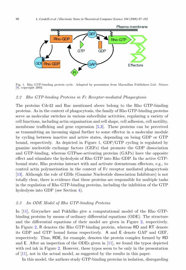
Fig. 1. Rho GTP-binding protein cycle. Adapted by permission from Macmillan Publishers Ltd: Nature[9], copyright 2002.

2.2 Rho GTP-binding Proteins in Fc Receptor-mediated Phagocytosis

The proteins Cdc42 and Rac mentioned above belong to the Rho GTP-bindingproteins. As in the context of phagocytosis, the family of Rho GTP-binding proteinsserve as molecular switches in various subcellular activities, regulating a variety ofcell functions, including actin organisation and cell shape, cell adhesion, cell motility,membrane trafficking and gene expression [5,3]. These proteins can be perceivedas transmitting an incoming signal further to some effector in a molecular moduleby cycling between inactive and active states, depending on being GDP or GTPbound, respectively. As depicted in Figure 1, GDP/GTP cycling is regulated byguanine nucleotide exchange factors (GEFs) that promote the GDP dissociationand GTP-binding, whereas GTPase-activating proteins (GAPs) have the oppositeeffect and stimulate the hydrolysis of Rho GTP into Rho GDP. In the active GTP-bound state, Rho proteins interact with and activate downstream effectors, e.g., tocontrol actin polymerisation in the context of Fc receptor mediated phagocytosis[13]. Although the role of GDIs (Guanine Nucleotide dissociation Inhibitors) is nottotally clear, there is evidence that these proteins are responsible for multiple tasksin the regulation of Rho GTP-binding proteins, including the inhibition of the GTPhydrolysis into GDP (see Section 4).

2.3 An ODE Model of Rho GTP-binding Proteins

In [11], Goryachev and Pokhilko give a computational model of the Rho GTP-binding proteins by means of ordinary differential equations (ODE). The structureand the differential equations of their model are given in Figure 2, respectively.In Figure 2, R denotes the Rho GTP-binding protein, whereas RD and RT denoteits GDP and GTP bound forms respectively. A and E denote GAP and GEF,respectively. Thus, RDE, for example, denotes the protein complex formed by RDand E. After an inspection of the ODEs given in [11], we found the typos depictedwith red ink in Figure 2. However, these typos seem to be only in the presentationof [11], not in the actual model, as suggested by the results in this paper.

In this model, the authors study GTP-binding proteins in isolation, disregarding


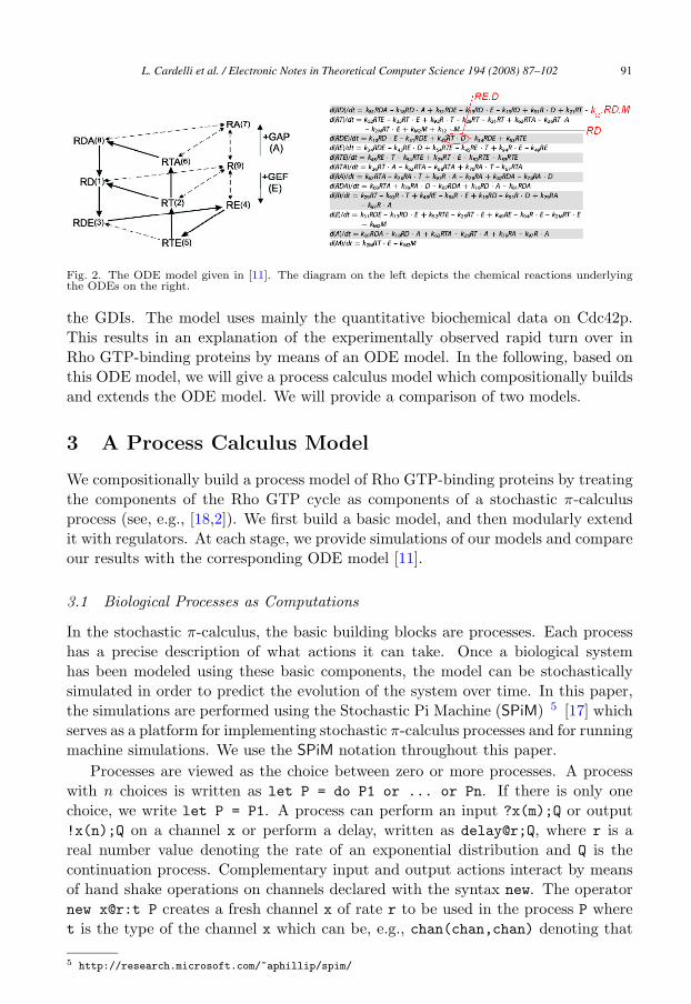
Fig. 2. The ODE model given in [11]. The diagram on the left depicts the chemical reactions underlyingthe ODEs on the right.

the GDIs. The model uses mainly the quantitative biochemical data on Cdc42p.This results in an explanation of the experimentally observed rapid turn over inRho GTP-binding proteins by means of an ODE model. In the following, based onthis ODE model, we will give a process calculus model which compositionally buildsand extends the ODE model. We will provide a comparison of two models.

3 A Process Calculus Model

We compositionally build a process model of Rho GTP-binding proteins by treatingthe components of the Rho GTP cycle as components of a stochastic π-calculusprocess (see, e.g., [18,2]). We first build a basic model, and then modularly extendit with regulators. At each stage, we provide simulations of our models and compareour results with the corresponding ODE model [11].

3.1 Biological Processes as Computations

In the stochastic π-calculus, the basic building blocks are processes. Each processhas a precise description of what actions it can take. Once a biological systemhas been modeled using these basic components, the model can be stochasticallysimulated in order to predict the evolution of the system over time. In this paper,the simulations are performed using the Stochastic Pi Machine (SPiM) 5 [17] whichserves as a platform for implementing stochastic π-calculus processes and for runningmachine simulations. We use the SPiM notation throughout this paper.

Processes are viewed as the choice between zero or more processes. A processwith n choices is written as let P = do P1 or ... or Pn. If there is only onechoice, we write let P = P1. A process can perform an input ?x(m);Q or output!x(n);Q on a channel x or perform a delay, written as delay@r;Q, where r is areal number value denoting the rate of an exponential distribution and Q is thecontinuation process. Complementary input and output actions interact by meansof hand shake operations on channels declared with the syntax new. The operatornew x@r:t P creates a fresh channel x of rate r to be used in the process P wheret is the type of the channel x which can be, e.g., chan(chan,chan) denoting that

5 http://research.microsoft.com/~aphillip/spim/


(i) (ii.)

(iii.) (iv.)

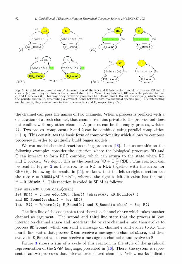
Fig. 3. Graphical representation of the evolution of the RD and E interaction model. Processes RD and Ecoexist (i.), and they can interact on channel share (ii.). When they interact, RD sends the private channele, and E receives it. This way, they evolve to processes RD Bound and E Bound, respectively, which sharethe private channel e, resembling a covalent bond between two bio-chemical species (iii.). By interactingon channel e, they evolve back to the processes RD and E, respectively (iv.).

the channel can pass the names of two channels. When a process is prefixed with adeclaration of a fresh channel, that channel remains private to the process and doesnot conflict with any other channel. A process can be the empty process, written(). Two process components P and Q can be combined using parallel compositionP | Q. This constitutes the basic form of compositionality which allows to composeprocesses in order to gradually build bigger models.

We can model chemical reactions using processes [18]. Let us see this on thefollowing example: consider the situation where the biological processes RD andE can interact to form RDE complex, which can return to the state where RDand E coexist. We depict this as the reaction RD + E

r�r′

RDE . This reaction canbe read in Figure 2 as the arrow from RD to RDE together with the arrow forGEF (E). Following the results in [11], we know that the left-to-right direction hasthe rate r = 0.0054μM−1.min−1, whereas the right-to-left direction has the rater′ = 0.136min−1. This reaction is coded in SPiM as follows:

new [email protected]:chan(chan)let RD() = ( new [email protected]: chan() !share(e); RD_Bound(e) )and RD_Bound(e:chan) = !e; RD()let E() = ?share(e); E_Bound(e) and E_Bound(e:chan) = ?e; E()

The first line of the code states that there is a channel share which takes anotherchannel as argument. The second and third line state that the process RD caninteract on channel share and broadcast the private channel e, and then evolve toprocess RD_Bound, which can send a message on channel e and evolve to RD. Thefourth line states that process E can receive a message on channel share, and thenevolve to E_Bound which can receive a message on channel e and evolve to E.

Figure 3 shows a run of a cycle of this reaction in the style of the graphicalrepresentation of the SPiM language, presented in [16]. There, the system is repre-sented as two processes that interact over shared channels. Yellow marks indicate


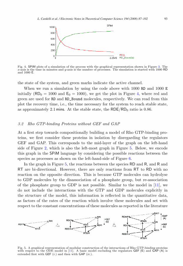
Fig. 4. SPiM plots of a simulation of the process with the graphical representation shown in Figure 3. Thex-axis is the time in minutes and y-axis is the number of processes. The simulation is started with 1000 RDand 1000 E.

the state of the system, and green marks indicate the active channel.When we run a simulation by using the code above with 1000 RD and 1000 E

initially (RD0 = 1000 and E0 = 1000), we get the plot in Figure 4, where red andgreen are used for RD and RD_Bound molecules, respectively. We can read from thisplot the recovery time, i.e., the time necessary for the system to reach stable state,as approximately 2.1 mins. At the stable state, the RDE/RD0 ratio is 0.86.

3.2 Rho GTP-binding Proteins without GEF and GAP

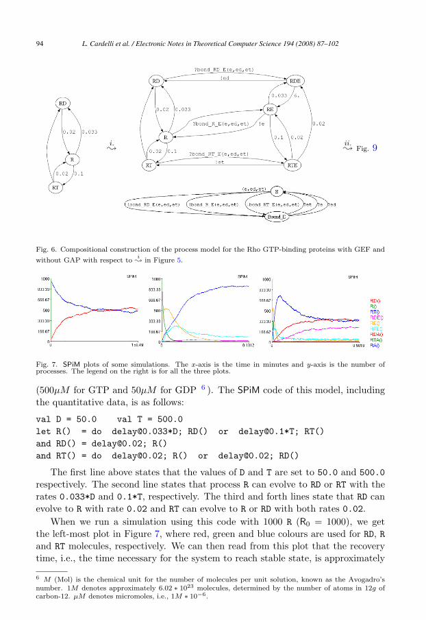
At a first step towards compositionally building a model of Rho GTP-binding pro-teins, we first consider these proteins in isolation by disregarding the regulatorsGEF and GAP. This corresponds to the mid-layer of the graph on the left-handside of Figure 2, which is also the left-most graph in Figure 5. Below, we encodethis graph in the SPiM language by considering the possible reactions between thespecies as processes as shown on the left-hand-side of Figure 6.

In the graph in Figure 5, the reactions between the species RD and R, and R andRT are bi-directional. However, there are only reactions from RT to RD with noreaction on the opposite direction. This is because GTP molecules can hydrolyseto GDP molecules by the disassociation of a phosphate group, but re-associationof the phosphate group to GDP is not possible. Similar to the model in [11], wedo not include the interactions with the GTP and GDP molecules explicitly inthe structure of the model, this information is reflected in the quantitative data,as factors of the rates of the reaction which involve these molecules and set withrespect to the constant concentrations of these molecules as reported in the literature

i.�

ii.�

Fig. 5. A graphical representation of modular construction of the interactions of Rho GTP-binding proteinswith respect to the ODE model in [11]. A basic model excluding the regulators GEF (E) and GAP (A) isextended first with GEF (i.) and then with GAP (ii.).


i.�

ii.� Fig. 9

Fig. 6. Compositional construction of the process model for the Rho GTP-binding proteins with GEF and

without GAP with respect toi

� in Figure 5.

Fig. 7. SPiM plots of some simulations. The x-axis is the time in minutes and y-axis is the number ofprocesses. The legend on the right is for all the three plots.

(500μM for GTP and 50μM for GDP 6 ). The SPiM code of this model, includingthe quantitative data, is as follows:

val D = 50.0 val T = 500.0let R() = do [email protected]*D; RD() or [email protected]*T; RT()and RD() = [email protected]; R()and RT() = do [email protected]; R() or [email protected]; RD()

The first line above states that the values of D and T are set to 50.0 and 500.0respectively. The second line states that process R can evolve to RD or RT with therates 0.033*D and 0.1*T, respectively. The third and forth lines state that RD canevolve to R with rate 0.02 and RT can evolve to R or RD with both rates 0.02.

When we run a simulation using this code with 1000 R (R0 = 1000), we getthe left-most plot in Figure 7, where red, green and blue colours are used for RD, Rand RT molecules, respectively. We can then read from this plot that the recoverytime, i.e., the time necessary for the system to reach stable state, is approximately

6 M (Mol) is the chemical unit for the number of molecules per unit solution, known as the Avogadro’snumber. 1M denotes approximately 6.02 ∗ 1023 molecules, determined by the number of atoms in 12g ofcarbon-12. μM denotes micromoles, i.e., 1M ∗ 10−6.


90 mins. At the stable state, the RT/R0 ratio is 0.5.

3.3 Rho GTP-binding Proteins with GEF and without GAP

We extend the Rho GTP-binding protein process model, given in Subsection 3.2, to aprocess that also models GEF regulation. This corresponds to the middle diagramin Figure 5 and process model given in Figure 6. Here, we have two interactingprocesses, one for the Rho GTP-binding protein, which extends the process modelgiven in the previous subsection, and one for GEF (the E process). The SPiM codeof the model in Subsection 3.4 extends the code of this model, however that codecan also be used for this model by taking the initial number of A (GAP in Figure 2)as 0. When we run a simulation using this code with 1000 R and 1000 E processes(R0 = 1000 and E0 = 1000), we get the middle plot in Figure 7, where red, green,blue, pink, yellow, and light blue colours are used for RD, R, RT, RDE, RE, and RTEmolecules, respectively. We can then read from this plot that the recovery time, i.e.,the time necessary for the system to reach stable state, is approximately 0.12mins.At the stable state, the RT/R0 ratio is 0.87.

In order to compare our process model with the ODE model given in [11], weran the SPiM simulations on a range of initial number of molecules, where R0 and E0

range between 10−2μM and 106μM . In these simulations, the rate values are givenwith the unit μM−1. Because of this, we encode 1μM of a species as 1 instance ofthe process in the model at the start of the simulation. For instance, when we startthe simulation with E0 = 1000, this corresponds to 1000μM in the ODE model. Inorder to be able to run simulations for the situations where the initial concentrationof species are too low for meaningful stochastic simulations or too high from thepoint of view of computational resources, we do a scaling by means of a factoringconstant. This scaling can be seen to be performed on the underlying chemicalreactions, that is, we divide the rates of the underlying binary chemical reactionsand multiply the initial concentrations of the species with a factoring constant [20].For instance, in order to run a simulation for the case where there are 10−2μM of Rand 10−2μM of E, we scale the rate values by a factor of 104, which allows to givethe initial values as 10−2 ∗ 104 = 102. For this purpose, we divide the rates of theinteraction channels in the process model with our scaling factor, e.g., 104.

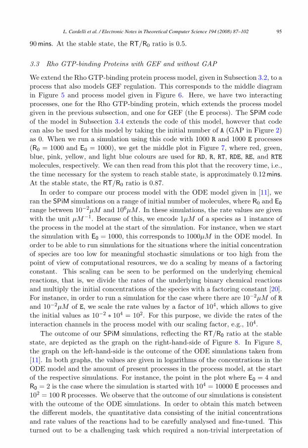
The outcome of our SPiM simulations, reflecting the RT/R0 ratio at the stablestate, are depicted as the graph on the right-hand-side of Figure 8. In Figure 8,the graph on the left-hand-side is the outcome of the ODE simulations taken from[11]. In both graphs, the values are given in logarithms of the concentrations in theODE model and the amount of present processes in the process model, at the startof the respective simulations. For instance, the point in the plot where E0 = 4 andR0 = 2 is the case where the simulation is started with 104 = 10000 E processes and102 = 100 R processes. We observe that the outcome of our simulations is consistentwith the outcome of the ODE simulations. In order to obtain this match betweenthe different models, the quantitative data consisting of the initial concentrationsand rate values of the reactions had to be carefully analysed and fine-tuned. Thisturned out to be a challenging task which required a non-trivial interpretation of


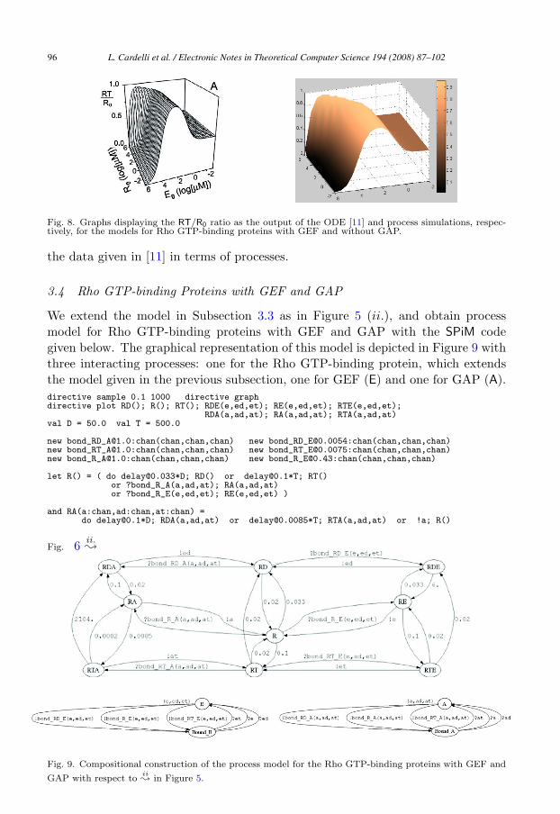
Fig. 8. Graphs displaying the RT/R0 ratio as the output of the ODE [11] and process simulations, respec-tively, for the models for Rho GTP-binding proteins with GEF and without GAP.

the data given in [11] in terms of processes.

3.4 Rho GTP-binding Proteins with GEF and GAP

We extend the model in Subsection 3.3 as in Figure 5 (ii.), and obtain processmodel for Rho GTP-binding proteins with GEF and GAP with the SPiM codegiven below. The graphical representation of this model is depicted in Figure 9 withthree interacting processes: one for the Rho GTP-binding protein, which extendsthe model given in the previous subsection, one for GEF (E) and one for GAP (A).directive sample 0.1 1000 directive graphdirective plot RD(); R(); RT(); RDE(e,ed,et); RE(e,ed,et); RTE(e,ed,et);

RDA(a,ad,at); RA(a,ad,at); RTA(a,ad,at)val D = 50.0 val T = 500.0

new [email protected]:chan(chan,chan,chan) new [email protected]:chan(chan,chan,chan)new [email protected]:chan(chan,chan,chan) new [email protected]:chan(chan,chan,chan)new [email protected]:chan(chan,chan,chan) new [email protected]:chan(chan,chan,chan)

let R() = ( do [email protected]*D; RD() or [email protected]*T; RT()or ?bond_R_A(a,ad,at); RA(a,ad,at)or ?bond_R_E(e,ed,et); RE(e,ed,et) )

and RA(a:chan,ad:chan,at:chan) =do [email protected]*D; RDA(a,ad,at) or [email protected]*T; RTA(a,ad,at) or !a; R()

Fig. 6 ii.�

Fig. 9. Compositional construction of the process model for the Rho GTP-binding proteins with GEF and

GAP with respect toii� in Figure 5.


and RE(e:chan,ed:chan,et:chan) =do [email protected]*D; RDE(e,ed,et) or [email protected]*T; RTE(e,ed,et) or !e; R()

and RT() = ( do [email protected]; R() or [email protected]; RD()or ?bond_RT_A(a,ad,at); RTA(a,ad,at)or ?bond_RT_E(e,ed,et); RTE(e,ed,et) )

and RTA(a:chan,ad:chan,at:chan) =do [email protected]; RA(a,ad,at) or [email protected]; RDA(a,ad,at) or !at; RT()

and RTE(e:chan,ed:chan,et:chan) =do [email protected]; RDE(e,ed,et) or [email protected]; RE(e,ed,et) or !et; RT()

and RD() = ( do [email protected]; R() or ?bond_RD_A(a,ad,at); RDA(a,ad,at)or ?bond_RD_E(e,ed,et); RDE(e,ed,et) )

and RDA(a:chan,ad:chan,at:chan) = do [email protected]; RA(a,ad,at) or !ad; RD()

and RDE(e:chan,ed:chan,et:chan) = do [email protected]; RE(e,ed,et) or !ed; RD()

let A() = ( new [email protected]:chan new [email protected]:chan new [email protected]:chando !bond_R_A(a,ad,at); Bound_A(a,ad,at)or !bond_RT_A(a,ad,at); Bound_A(a,ad,at)or !bond_RD_A(a,ad,at); Bound_A(a,ad,at) )

and Bound_A(a:chan,ad:chan,at:chan) = do ?a; A() or ?ad; A() or ?at; A()

let E() = ( new [email protected]:chan new [email protected]:chan new [email protected]:chando !bond_R_E(e,ed,et); Bound_E(e,ed,et)or !bond_RT_E(e,ed,et); Bound_E(e,ed,et)or !bond_RD_E(e,ed,et); Bound_E(e,ed,et) )

and Bound_E(e:chan,ed:chan,et:chan) = do ?e; E() or ?ed; E() or ?et; E()

run 1000 of R() run 10 of A() run 1000 of E()

When we run a simulation using this code with 1000 R, 10 A and 1000 E processes(R0 = 1000, A0 = 10 and E0 = 1000), we get the right-most plot in Figure 7. Wecan then read from this plot that the recovery time is approximately 0.5mins. Atthe stable state, the RT/R0 ratio is 0.35.

In order to compare this model with the model in [11], we ran simulations ona range of initial number of molecules, where R0 is 1000 and E0 ranges between10−1μM and 104μM , and A0 ranges between 10−2μM and 102μM . For some sim-ulations, we performed a scaling as described for the simulations in Subsection 3.3.

The outcome of our simulations are depicted as the graph on the right-hand-side of Figure 10, where the graph on the left-hand-side is the outcome of the ODEsimulations taken from [11]. In both graphs, the values are given in logarithmsof the concentrations in the ODE model and the amount of present species in theprocess model, at the beginning of the respective simulations. Again, the outcomeof these simulations is consistent with the outcome of the ODE simulations.

4 Extending the Model with Effectors and GDI

Besides the regulators GEF and GAP, the Rho GTP cycle depicted in Figure 1 isalso affected by the interactions with the effectors and another regulator called GDI.The effectors of the Rho GTP-binding proteins, e.g., WASP (also in the context ofphagocytosis), change their structural conformation and gain the ability to bind toother proteins while they are associated with the active GTP-bound Rho proteinattached to the membrane. The GDIs (Guanine-nucleotide Dissociation Inhibitors)form a class of regulatory proteins for the Rho GTP cycle [6,7,8]. GDIs play two


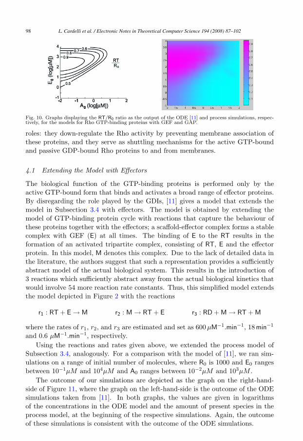
Fig. 10. Graphs displaying the RT/R0 ratio as the output of the ODE [11] and process simulations, respec-tively, for the models for Rho GTP-binding proteins with GEF and GAP.

roles: they down-regulate the Rho activity by preventing membrane association ofthese proteins, and they serve as shuttling mechanisms for the active GTP-boundand passive GDP-bound Rho proteins to and from membranes.

4.1 Extending the Model with Effectors

The biological function of the GTP-binding proteins is performed only by theactive GTP-bound form that binds and activates a broad range of effector proteins.By disregarding the role played by the GDIs, [11] gives a model that extends themodel in Subsection 3.4 with effectors. The model is obtained by extending themodel of GTP-binding protein cycle with reactions that capture the behaviour ofthese proteins together with the effectors; a scaffold-effector complex forms a stablecomplex with GEF (E) at all times. The binding of E to the RT results in theformation of an activated tripartite complex, consisting of RT, E and the effectorprotein. In this model, M denotes this complex. Due to the lack of detailed data inthe literature, the authors suggest that such a representation provides a sufficientlyabstract model of the actual biological system. This results in the introduction of3 reactions which sufficiently abstract away from the actual biological kinetics thatwould involve 54 more reaction rate constants. Thus, this simplified model extendsthe model depicted in Figure 2 with the reactions

r1 : RT + E → M r2 : M → RT + E r3 : RD + M → RT + M

where the rates of r1, r2, and r3 are estimated and set as 600 μM−1.min−1, 18 min−1

and 0.6 μM−1.min−1, respectively.Using the reactions and rates given above, we extended the process model of

Subsection 3.4, analogously. For a comparison with the model of [11], we ran sim-ulations on a range of initial number of molecules, where R0 is 1000 and E0 rangesbetween 10−1μM and 104μM and A0 ranges between 10−2μM and 103μM .

The outcome of our simulations are depicted as the graph on the right-hand-side of Figure 11, where the graph on the left-hand-side is the outcome of the ODEsimulations taken from [11]. In both graphs, the values are given in logarithmsof the concentrations in the ODE model and the amount of present species in theprocess model, at the beginning of the respective simulations. Again, the outcomeof these simulations is consistent with the outcome of the ODE simulations.


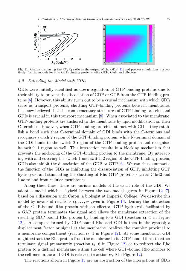
Fig. 11. Graphs displaying the RT/R0 ratio as the output of the ODE [11] and process simulations, respec-tively, for the models for Rho GTP-binding proteins with GEF, GAP and effectors.

4.2 Extending the Model with GDIs

GDIs were initially identified as down-regulators of GTP-binding proteins due totheir ability to prevent the dissociation of GDP or GTP from the GTP-binding pro-teins [6]. However, this ability turns out to be a crucial mechanism with which GDIsserve as transport proteins, shuttling GTP-binding proteins between membranes.It is now believed that the complementary structures of GTP-binding proteins andGDIs is crucial in this transport mechanism [8]. When associated to the membrane,GTP-binding proteins are anchored to the membrane by lipid modification on theirC-terminus. However, when GTP-binding proteins interact with GDIs, they estab-lish a bond such that C-terminal domain of GDI binds with the C-terminus andrecognises switch 2 region of the GTP-binding protein, while N-terminal domain ofthe GDI binds to the switch 2 region of the GTP-binding protein and recognisesits switch 1 region as well. This interaction results in a blocking mechanism thatprevents the anchoring of the GTP-binding protein to the membrane. By interact-ing with and covering the switch 1 and switch 2 region of the GTP-binding protein,GDIs also inhibit the dissociation of the GDP or GTP [6]. We can thus summarisethe function of the GDIs as inhibiting the disassociation of GDP, inhibiting GTPhydrolysis, and stimulating the shuttling of Rho GTP proteins such as Cdc42 andRac to and from cellular membranes.

Along these lines, there are various models of the exact role of the GDI. Weadopt a model which is hybrid between the two models given in Figure 12 [7],based on a discussion with Caron, a biologist at Imperial College. We describe thismodel by means of reactions r4, . . . , r7 given in Figure 13. During the interactionof the GTP-bound Rho protein with an effector, GTP hydrolysis facilitated bya GAP protein terminates the signal and allows the membrane extraction of theresulting GDP-bound Rho protein by binding to a GDI (reaction r4, 5 in Figure12). A complex formed by GDP-bound Rho and GDI is then in the cytosol; adisplacement factor or signal at the membrane localizes the complex proximal toa membrane compartment (reaction r5, 1 in Figure 12). At some membrane, GDImight extract the Rho protein from the membrane in its GTP-bound form to eitherterminate signal prematurely (reaction r6, 6 in Figure 12) or to redirect the Rhoprotein to a distinct membrane within the cell where GTP-bound Rho anchors tothe cell membrane and GDI is released (reaction r7, 9 in Figure 12).

The reactions shown in Figure 13 are an abstraction of the interactions of GDIs


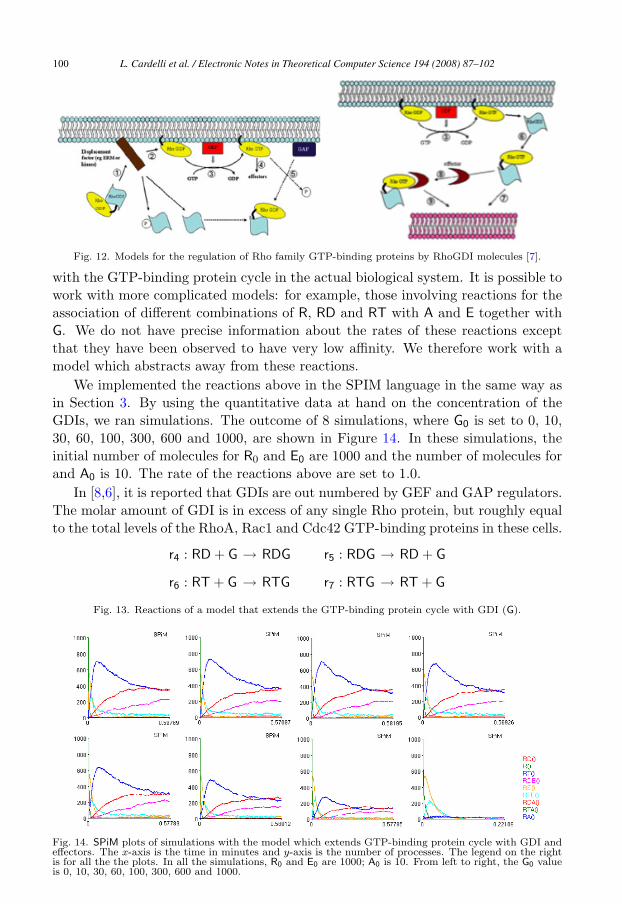
Fig. 12. Models for the regulation of Rho family GTP-binding proteins by RhoGDI molecules [7].

with the GTP-binding protein cycle in the actual biological system. It is possible towork with more complicated models: for example, those involving reactions for theassociation of different combinations of R, RD and RT with A and E together withG. We do not have precise information about the rates of these reactions exceptthat they have been observed to have very low affinity. We therefore work with amodel which abstracts away from these reactions.

We implemented the reactions above in the SPIM language in the same way asin Section 3. By using the quantitative data at hand on the concentration of theGDIs, we ran simulations. The outcome of 8 simulations, where G0 is set to 0, 10,30, 60, 100, 300, 600 and 1000, are shown in Figure 14. In these simulations, theinitial number of molecules for R0 and E0 are 1000 and the number of molecules forand A0 is 10. The rate of the reactions above are set to 1.0.

In [8,6], it is reported that GDIs are out numbered by GEF and GAP regulators.The molar amount of GDI is in excess of any single Rho protein, but roughly equalto the total levels of the RhoA, Rac1 and Cdc42 GTP-binding proteins in these cells.

r4 : RD + G → RDG

r6 : RT + G → RTG

r5 : RDG → RD + G

r7 : RTG → RT + G

Fig. 13. Reactions of a model that extends the GTP-binding protein cycle with GDI (G).

Fig. 14. SPiM plots of simulations with the model which extends GTP-binding protein cycle with GDI andeffectors. The x-axis is the time in minutes and y-axis is the number of processes. The legend on the rightis for all the the plots. In all the simulations, R0 and E0 are 1000; A0 is 10. From left to right, the G0 valueis 0, 10, 30, 60, 100, 300, 600 and 1000.


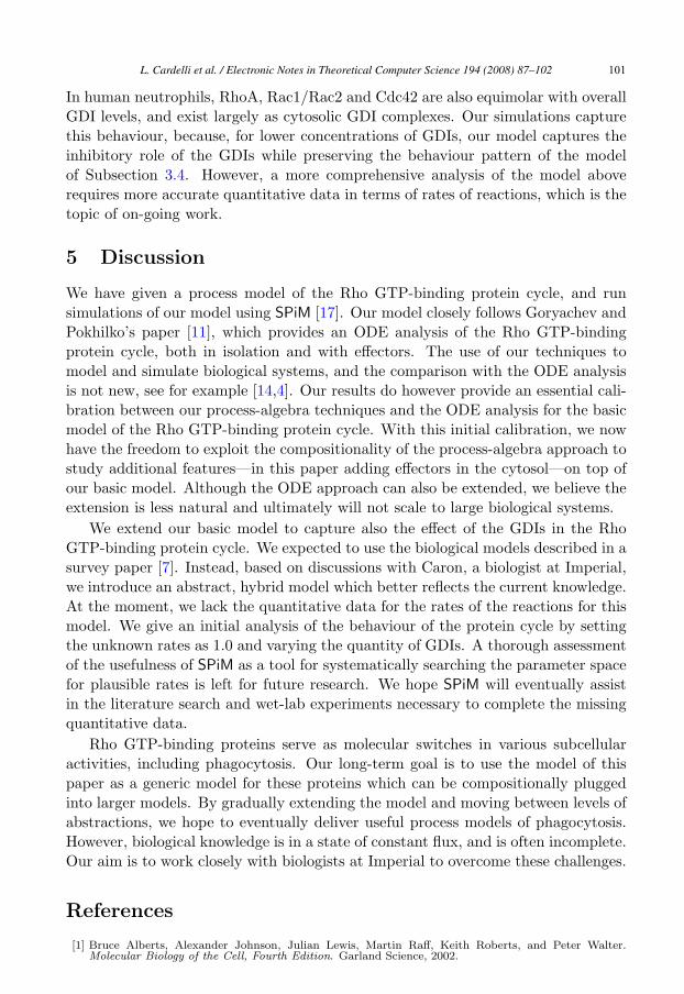
In human neutrophils, RhoA, Rac1/Rac2 and Cdc42 are also equimolar with overallGDI levels, and exist largely as cytosolic GDI complexes. Our simulations capturethis behaviour, because, for lower concentrations of GDIs, our model captures theinhibitory role of the GDIs while preserving the behaviour pattern of the modelof Subsection 3.4. However, a more comprehensive analysis of the model aboverequires more accurate quantitative data in terms of rates of reactions, which is thetopic of on-going work.

5 Discussion

We have given a process model of the Rho GTP-binding protein cycle, and runsimulations of our model using SPiM [17]. Our model closely follows Goryachev andPokhilko’s paper [11], which provides an ODE analysis of the Rho GTP-bindingprotein cycle, both in isolation and with effectors. The use of our techniques tomodel and simulate biological systems, and the comparison with the ODE analysisis not new, see for example [14,4]. Our results do however provide an essential cali-bration between our process-algebra techniques and the ODE analysis for the basicmodel of the Rho GTP-binding protein cycle. With this initial calibration, we nowhave the freedom to exploit the compositionality of the process-algebra approach tostudy additional features—in this paper adding effectors in the cytosol—on top ofour basic model. Although the ODE approach can also be extended, we believe theextension is less natural and ultimately will not scale to large biological systems.

We extend our basic model to capture also the effect of the GDIs in the RhoGTP-binding protein cycle. We expected to use the biological models described in asurvey paper [7]. Instead, based on discussions with Caron, a biologist at Imperial,we introduce an abstract, hybrid model which better reflects the current knowledge.At the moment, we lack the quantitative data for the rates of the reactions for thismodel. We give an initial analysis of the behaviour of the protein cycle by settingthe unknown rates as 1.0 and varying the quantity of GDIs. A thorough assessmentof the usefulness of SPiM as a tool for systematically searching the parameter spacefor plausible rates is left for future research. We hope SPiM will eventually assistin the literature search and wet-lab experiments necessary to complete the missingquantitative data.

Rho GTP-binding proteins serve as molecular switches in various subcellularactivities, including phagocytosis. Our long-term goal is to use the model of thispaper as a generic model for these proteins which can be compositionally pluggedinto larger models. By gradually extending the model and moving between levels ofabstractions, we hope to eventually deliver useful process models of phagocytosis.However, biological knowledge is in a state of constant flux, and is often incomplete.Our aim is to work closely with biologists at Imperial to overcome these challenges.

References

[1] Bruce Alberts, Alexander Johnson, Julian Lewis, Martin Raff, Keith Roberts, and Peter Walter.Molecular Biology of the Cell, Fourth Edition. Garland Science, 2002.


[2] Ralf Blossey, Luca Cardelli, and Andrew Phillips. A compositional approach to the stochastic dynamicsof gene networks. Transactions in Computational Systems Biology, 3939:99–122, 2006.

[3] Xose R. Bustelo, Vincent Sauzeau, and Inmaculada M. Berenjeno. Gtp-binding proteins of the rho/racfamily: regulation, effectors and function in vivo. BioEssays, 29:356–370, 2007.

[4] Luca Cardelli. On process rate semantics. Theoretical Computer Science, 2007. to appear.

[5] Giovanni Chimini and Philippe Chavrier. Function of Rho family proteins in actin dynamics duringphagocytosis and engulfment. Nature Cell Biology, 2:191–196, 2000.

[6] Celine DerMardirossian and Gary M. Bokoch. GDIs: central regulatory molecules in Rho GTPaseactivation. TRENDS in Cell Biology, 15(7):356–363, 2005.

[7] Athanassios Dovas and John R. Couchman. RhoGDI: Multiple functions in the regulation of rho familygtpase activities. Biochemistry Journal, 390:1–9, 2005.

[8] Estelle Dransart, Birgitta Olofsson, and Jacqueline Cherfils. RhoGDIs revisted: Novel roles in rhoregulation. Traffic, 6:957–966, 2005.

[9] Sandrine Etienne-Manneville and Alan Hall. Rho GTPases in cell biology. Nature, 420:629–635, 2002.

[10] Erick Garcia-Garcia and Carlos Rosales. Signal transduction during fc receptor-mediated phagocytosis.Journal of Leukocyte Biology, 72:1092–1108, 2002.

[11] Andrew B. Goryachev and Alexandra V. Pokhilko. Computational model explains highactivity and rapid cycling of rho gtpases within protein complexes. PLOS ComputationalBiology, 2:1511–1521, 2006. For the license terms of the figures adapted from this work, seehttp://creativecommons.org/licenses/by/2.5/.

[12] A.B. Hall, M. A. Gakidis, M Glogauer, J.L. Wilsbacher, S Gao, W. Swat, and J.S. Brugge. Requirementsfor vav guanine nucleotide exchange factors and rho gtpases in fcγr- and complement-mediatedphagocytosis. Immunity, 24:305–316, 2006.

[13] Aron B. Jaffe and Alan Hall. Rho GTPases: Biochemistry and biology. Annual Review of Cell andDevelopmental Biology, 21:247–269, 2005.

[14] P. Lecca and C. Priami. Cell cycle control in eukaryotes: A BioSpi model. In Proc. Workshop onConcurrent Models in Molecular Biology (BioConcur’03), ENTCS. Elsevier, 2003.

[15] J. C. Patel, A. Hall, and E. Caron. Vav regulates activation of rac but not cdc42 during FcγR-mediatedphagocytosis. Molecular Biology of the Cell, 13:1215–1226, 2002.

[16] A. Phillips, L. Cardelli, and G. Castagna. A graphical representation for biological processes in thestochastic pi-calculus. Transactions in Computational Systems Biology, 4230:123–152, 2006.

[17] Andrew Phillips and Luca Cardelli. Efficient simulation of biological processes in the stochastic pi-calculus. submitted, 2007.

[18] C. Priami, A. Regev, E. Shapiro, and W. Silverman. Application of a stochastic name-passing calculusto representation and simulation of molecular processes. Information Processing Letters, 80, 2001.

[19] Joel A. Swanson and Adam D. Hoppe. Cdc42, Rac1, and Rac2 display distinct patterns of activationduring phagocytosis. Molecular Biology of the Cell, 15(8):3509–3519, 2004.

[20] O. Wolkenhauer, M. Ullah, W. Kolch, and Cho K.H. Modeling and simulation of intracellular dynamics:choosing an appropriate framework. IEEE Trans. Nanobioscience, 3:200–207, 2004.


a process model of rho gtp-binding proteins in the context of phagocytosis

Documents