a program data flow analysis procedure - turing award · programming techniques g. manacher, s....

Programming Techniques

G. Manacher, S. Graham Editors

A Program Data Flow Analysis Procedure F.E. Allen and J. Cocke IBM Thomas J. Watson Research Center

The global data relationships in a program can be exposed and codified by the static analysis methods described in this paper. A procedure is given which determines all the definitions which can possibly "reach" each node of the control flow graph of the program and all the definitions that are "live" on each edge of the graph. The procedure uses an "interval" ordered edge listing data structure and handles reducible and irreducible graphs indistinguishably.

Key Words and Phrases: program optimization, data flow analysis, flow graphs, algorithms, compilers

CR Categories: 4.12, 5.24

Copyright © 1976, Association for Computing Machinery, Inc. General permission to republish, but not for profit, all or part of this material is granted provided that ACM's copyright notice is given and that reference is made to the publication, to its date of issue, and to the fact that reprinting privileges were granted by permission of the Association for Computing Machinery.

Authors' address: IBM Thomas J. Watson Research Center, P.O. Box 218, Yorktown Heights, N.Y. 10598.

137

1. Introduction

Given a definition of a data item in a program, it is frequently desirable to know what uses might be affected by the particular definition. The inverse is also true: for a given use the definitions of data items which can potentially supply values to it are of interest. Such data flow relationships, or "def-use" relationships, as they are often called, can be deduced by a static, com- pile time analysis of a program. A procedure for determining the information required for these def-use relationships is given in this paper.

Another data flow relationship which is also of interest is the following: given a program point (instruction) what data definitions are "live" at that point, that is, what data definitions given before this point are used after this point. This information is of interest, for example, when assigning index registers: data which is live at a point in a program might profitably be held in a index register at that point. The procedure given here includes the analysis required to expose live information.

In order to more precisely define the relationships derived by the procedure and to motivate the method used, certain basic concepts and constructs must be defined. This is done in Section 2. Section 3 gives the basic data flow analysis method and concludes with a brief survey of various methods. Section 4 discusses "intervals," the control flow basis used by the procedure given in this paper. In Sections 5 and 6 the procedure is described, with the latter section giving a PL//I implementation of the procedure. The paper concludes with a sum- mary and an extended bibliography.

The data flow analysis procedure given here has been implemented and used in a PL/I oriented, Experimental Compiling System. Dr. Kenneth Kennedy of Rice Uni- versity is responsible for the "live" analysis algorithm. Mr. Richard Stasko of IaM contributed to some of the data structure ideas used in the implementation. Dr. Jeffrey Ullman of Princeton, Dr. Matthew Hecht of the University of Maryland, Dr. Gary Kildall of the Naval Post Graduate School, Dr. Marvin Schaefer of SDC, Dr. Jacob Schwartz of New York University, and others have also made substantial contributions to this

area.

2. Context and Problem Statement

Our approach is to derive and express the data flow relationships in terms of the control flow graph [3, 7]

Communications March 1976 of Volume 19 the ACM Number 3

of the program. For the purposes of this paper the control flow graph G of a program is a connected, directed graph having a single entry node no. G consists of a set of nodes, N = {no, nl , n ._ , , . . . , m}, representing sequences of program instructions and a set of edges, E, of ordered pairs of nodes representing the flow of control.

f Fig. 1.

The graph depicted in Figure 1 has

no = 1; N = { 1, 2, 3 , . . . , 7} (the numbering is arbitrary); and E = { (1, 2), (1, 7), (2, 3), etc. }

The immediate successors of a node n~ are all of the nodes ni for which (n~, n~) is an edge in E. The immediate predecessors of node nj are all of the nodes n~ for which (n~, n~) is an edge in E. A path is an ordered sequence of nodes (nl , n _ ~ , . . . , nk) and their connect- ing edges in which each n~ is an immediate predecessor of n~+~. A closed path or cycle is a path in which the first and last nodes are the same. The successors of a node n~ are all of the nodes nj for which there exists a path (ni , . . . , n j). The predecessors of a node nj are all of the nodes n~ for which there exists a path f rom n~ to n j .

We can now more precisely define the data flow relationships we are interested in. A data definition is an expression or that part of an expression which modifies a data item. A data use is an expression or that part of an expression which references a data item without modify- •ng it. A data definition potentially affects a use if the data items are the same and the result of the definition is available to the use. In order to determine which definitions affect which uses, two types of expression relationships can be distinguished: those relationships which exist between expressions within straight line sequences of code and those which exist in the context of control flow. Methods for finding and codifying the relationships in straight line sequences are relatively easy and will not be given in this paper. (Cocke and Schwartz [8] contains a discussion of one excellent m e t h o d - - value numbering.)

In this paper we are concerned with determining the data flow relationships that exist between collections of instructions. Two particularly interesting collections are now defined.

A basic block is a linear sequence of program instructions having one entry point (the first instruction exe- cuted) and one exit point (the last instruction exe- cuted). The nodes of the control flow graph can represent the basic blocks of a program. A node can also represent an extended basic block: a sequence of program instructions each of which, with the exception of the first instruction, has one and only one immediate predecessor and that predecessor precedes it, ( though not necessarily immediately) in the extended basic block. An extended basic block can be formed from the tree of basic blocks such as those derived for IF . . . T H E N . . . ELSE clauses. Again the data relationships internal to such blocks can be easily der ived- -a simple, stack oriented extension of the basic value numbering method can be used. The data methods in this paper will be given in terms of nodes which can represent basic blocks, extended basic blocks or, as will be seen, more complex collections of instructions and even entire procedures.

In order to introduce the basic data method more easily, several interesting sets of data flow information will now be defined in terms of basic blocks; some of these definitions will, however, later be revised to refer to the edges and paths on the control flow graph.

A locally available definition for a basic block is the last definition of the data item in the basic block.

Any definition of a data item X in the basic block is said to kill all definitions of the same data item reaching the basic block. Another way of expressing this is that all definitions of a data item which reach a basic block are preserved by the basic block if the data item is not redefined in the basic block.

A definition X in basic block n~ is said to reach basic block nk if 1. X i s a locally available definition f rom n~, 2. nk is a successor of n~, and 3. There is at least one path f rom n~ to nk which does

not contain a basic block having a redefinition of the same data item; that is, X is preserved on some path f rom n~ to nk. The data flow analysis procedure given in this paper

determines, among other things, the set of definitions, R~, that reach each node in the control flow graph.

A locally exposed use in a basic block is a use of a data item which is not preceded in the basic block by a definition of the data item.

A use of a data i tem is upwards exposed in basic block n~ if either it is locally upwards exposed f rom n~ or there exists a path ( n ~ . . . nk) such that the used data item is locally upwards exposed f rom nk and there does not exist a j , i < j < k, which contains a definition of the data item. The upwards exposed uses at a basic block n~ can be expressed as a set U~.

A definition, d, is active or live at basic block n~ if d reaches n~ (i.e. d C R~) and there is an upwards exposed use at n~ of the data i tem defined by d. The set L~

138 Communications March 1976 of Volume 19 the ACM Number 3

of definitions active or live at basic block nt is:

Lt = R~ n Ut .

(It is assumed that the elements of the R~ and U~ sets are encoded so that uses and definitions can be meaningfully intersected.) It should be noted that this definition differs slightly from some other definitions which have appeared in the literature [14, 19] in that it is the definition that is considered live rather than an exposed use of a data item.

Our procedure determines the upwards exposed uses U~ for each node nt and the definitions which are live on each edge in the graph--this latter is a slight variant on the form of definition for Lt just given but is in fact a more useful formulation.

Consider the example in Figure 2.

Fig. 2.

I =X

=X X=

X=

Subscripting the definitions of X in nodes 5 and 7 in order to distinguish them we get the values shown in Table I for R~, U~, and L~ for each node m. It is evident from this example that one of the interesting side bene- fits of deriving this information is that possible uninitial- ized uses of data items are found.

In Section 3 the basic methods for deriving the reach information are given.

3. Basic Data Flow Analysis Method

A fundamental item of information which must be derived is what definitions of data items reach each node from other nodes in the graph. It should be readily apparent that the set of definitions which reach a node nt is the union of the definitions available from the nodes which are immediate predecessors of n t . Letting At denote the set of available definitions at node n~ and

Table I.

Node Ri Ui Li

1 ~ x 2 X7 X X7 3 X~X7 X XsX7 4 X~X7 X X6X7 5 X~X7 ~ ,Q" 6 X~X7 X X~X7 7 X~X7 ~ JD"

R~ denote the set of definitions which reach ni then:

Rt = U Ap for all np which are immediate pred- (1) P ecessors of n i .

In order to formalize the construction of available definitions A, for a node n t , let DB~ be the set of locally available definitions of all data items defined in the node. Let PB~ be the set of all definitions in the program which are preserved through node i. Thus, if data item X is defined in the node then PB~ will not contain any definitions of X; on the other hand, if X is not defined anywhere in the node, then all the definitions of X in the program will be represented in PBt . A~ is constructed by formula (2).

At = (R , 17 PB, ) 13 D B , . (2)

(The B appended to P and D in the notation is used here and throughout the paper to indicate that the information expressed has been collected from the interior of the node.)

Consider the example in Figure 3. (The definitions are indexed with the node name in order to distinguish them.)

Fig. 3.

XI = YI = X 2 =

Y5 = X 4 =

The D B and P B sets for each node are:

DB~ = [)(1, Y~], PB1 = [,@'], DB~ = IX2], PB~ = [Y,, Y,], DB~ = [Ys], PB~ = IX1, )(2, X4], DB4 = IX4], PB4 = [Yx, Y,].

Using formulas (1) and (2) to process the nodes in the order 1, 2, 3, 4 yields:

R~ = [ / ] , A, = [X~, r d , R~ = [X~, Yd, A~ = [X~, Yd, R, = [X~, Yd, .4, = [X~, Y,], R, = [)(i, X2, r~], A4 = [)(4, Y,].

In the preceding example we were able to determine the definitions reaching each node in a single pass through the graph. This was possible because the graph did not contain cycles and we could therefore order the nodes so that a node was not processed until all of its predecessors were processed. Program control flow graphs usually contain cycles, however. There is no way in the presence of cycles to predictably determine the reaching information in one pass through the graph. In Figure 2, the definition of X in node 5 reaches node 3 (as well as 4, 5, 6, and 7). Since 3 is both a predecessor and successor of 5 a node ordering which allows reaching information to be propagated forward through the


pa ths of the g raph wi thou t visi t ing the nodes more than once does no t exist. In fact we need to say what ha ppe ns to fo rmula (1) when all of the predecessors o f a node have not been visi ted and hence all of the A¢ are no t known.

The s implest a lgo r i thm for der iv ing the reaching in fo rma t ion in a general con t ro l flow graph is given in the Basic Reach Algo r i t hm.

Basic Reach Algorithm

Inputs: the PBI and DBi for each node in the control flow graph Output: R~, the set of definitions which reach each node in the

graph. The set A~ of definitions available from each node is also created.

Method: 1. Initialize all of the A~ and R~ to the null set. 2. Perform step 3 while there is no change in any R~ or A, 3. Apply formula (1) followed by formula (2) to the nodes of

the graph. []

In an excel lent pape r on " A Unif ied A p p r o a c h to G l o b a l P r o g r a m O p t i m i z a t i o n , " K i lda l l [17] gives a genera l iza t ion of this a lgo r i thm and proves tha t the i n f o r m a t i o n does indeed stabil ize.

Clear ly the r ap id i ty with which the i n fo rma t ion stabil izes for a given graph very much depends on the order in which the nodes of the g raph are examined . In [10], Hech t and U l l m a n use a node o rde r ing es tab l i shed by app ly ing Ta r j an ' s dep th first spann ing tree a lgo r i t hm to the con t ro l f low graph. The p rocedure given in this p a p e r is based u p o n the use of in tervals [3, 4, 5, 7].

4. I n t e r v a l s

Given a node h, an interval I(h) is the max imal , single ent ry subg raph in which h is the only ent ry node and in which all c losed pa ths conta in h. The un ique in terva l node h is cal led the interval head or s imply the header node. A n interval can be expressed in te rms o f the nodes in it : I(h) = (n l , n2, . . . ,nm).

By selecting the p rope r set o f header nodes, a g raph m a y be pa r t i t i oned into a unique set of d is jo in t in tervals

= {/(ha), I(h~) . . . } . A n a lgo r i thm for such a par t i - t ion is:

Algorithm for Finding Intervals

1. Establish a set H for header nodes and initialize it with no, the unique entry node for the graph.

2. For h E Hfind l(h) as follows: 2.1. Put h in l(h) as the first element of l(h). 2.2. Add to l(h) any node all of whose immediate predecessors

are already in l(h). 2.3. Repeat 2.2 until no more nodes can be added to l(h).

3. Add to H all nodes in G which are not already in H and which are not in l(h) but which have immediate predecessors in l(h). Therefore a node is added to H the first time any (but not all) of its immediate predecessors become members of an interval.

4. Add l(h) to a set9 of intervals being developed. 5. Select the next unprocessed node in H and repeat steps 2, 3, 4, 5.

When there are no more unprocessed nodes in H, the procedure terminates. []

140

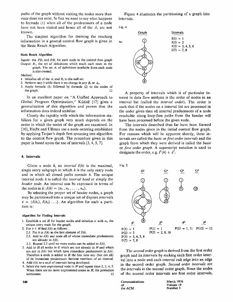
Figure 4 i l lustrates the pa r t i t i on ing o f a g raph into intervals .

Fig. 4.

Graph

()

Intervals

I(1) = 1 1(2) = 2 1(3) = 3, 4, 5, 6 1(7) = 7, 8

A p r o p e r t y of in tervals which is of pa r t i cu l a r interest in da t a f low analys is is the o rde r of nodes in an in terva l list (cal led the interval order). The o rde r is such tha t if the nodes on a in terva l list are p rocessed in the order given then all in terva l p redecessors of a node reachab le a long loop - f l ee pa ths f rom the header will have been processed before the given node.

The in tervals descr ibed thus far have been f o r m e d f rom the nodes given in the ini t ia l con t ro l f low graph . F o r reasons which will be a p p a r e n t shor t ly , these intervals are cal led the basic orfirst order intervals and the g raph f rom which they were der ived is cal led the basic or first order graph. A superscr ip t n o t a t i o n is used to des ignate the order , e.g. Ia(h) C aa.

Fig. 5.

G l G 2 G a G 4

91 9: 9 3

P(I ) = 1 P(1) = 1 P(1) = 1, 11 I'(2) = 2 I'(2) = 2, 9, 10 11(3) = 3, 4, 5, 6 11(7) = 7, 8'

@

9 4

I4(12) = 12

The second order graph is der ived f rom the first o rde r g raph and its in terva ls by m a k i n g each first o rde r in ter - val in to a node and each in te rva l exit edge in to an e d g e

in the second o rde r graph. Second order intervals are the in terva ls in the second o rde r g raph . Since the nodes of the second o rde r in terva ls a re first o rde r in tervals ,


this nesting can be used when determining inter-interval relationships. Successively higher order graphs can be derived until the nth order graph consists of a single node. Figure 5 illustrates such a sequence of derived graphs.

Not all graphs reduce to a single node by the iterative derivation indicated. A reducible graph is a graph whose nth order derived graph is a single node. A irreducible graph is a graph for which there does not exist an nth order derived graph consisting of a single node. Examples of irreducible graphs are given in Figure 6.

Fig. 6.

~AND (o) (b)

Methods for "splitting" (copying) certain nodes in an irreducible graph to produce an equivalent graph containing intervals exist [I, 7, 20]. Figure 7 illustrates

Fig. 7.

)

split graphs for the two irreducible forms given in Figure 6. It should be emphasized that splitting is an analysis technique and does not imply that the code in the nodes will appear more than once in the generated program. It is interesting to note that a program written by one of the authors to analyze the control flow of 75 "real" Fortran programs found that over 90 percent of the control flow graphs are reducible [7]. Further, Knuth [18] found no irreducible graphs in 50 Fortran programs.

The data flow analysis described in the next section is based on the interval construct just described.

5. Data Flow Analysis Using Intervals

By definition and by construction, an interval I(h) has only one entry, h, and all closed paths go through h. The definitions which reach each basic node in the interval could be determined, therefore, by formulas (1)

and (2) if all of the definitions which reach h, both from predecessors outside the interval and from predecessors in the interval, were known. These definitions can be found by a two-phase process.

The first phase of the process collects information and the second phase propagates it to the appropriate places. The first phase first collects information about what is defined and preserved in each first-ol der interval by processing the nodes in each interval in their interval order. The information collected is then posted to the node representing each interval in the second order derived graph. The second order intervals are then processed in the same way as the first order intervals and the process iterates.

For each interval at each level during the first phase, two items of information are collected from the nodes which comprise it (three items if the interval contains a loop) :

1. The definitions which are defined in the interval and locally available from it. This becomes the DB set for the node representing the interval in the next higher order graph.

2. The definitions which are preserved by the interval. This becomes the PB set for the representative node.

If the interval contains a loop, then a third item of information is collected: which definitions in the interval can reach the interval head. A set Rh associated with the interval head expresses this. During the second phase the Rh sets will make definition information available before the nodes containing the definitions have been processed. They are also used in the first phase to determine what definitions are available at interval exit points in cases such as depicted in Figure 8. There the

Fig. 8.

~ x=

definition of X in node 3 reaches the interval head and, assuming all definitions of X are preserved on the path from 1 through 2, X3 is available on exit from the interval. The effect of the first phase then is to percolate the influence of each node outwards into an increasingly more global context.

The second phase uses the information collected by the first phase and, by processing the graphs from high order to low order, generates the set of definitions reaching each node. Before processing an interval the Rh set associated with the header is modified to reflect those definitions that can reach the interval from outside. These are given in the R set generated for the interval's representative block in the next higher order graph. The modified Rh set is used to initiate processing the inter-


val. The order of the process is the interval o rde r - - t he

operat ions of the process are those given in formulas (1) and (2).

Since a node can represent collections of ins t ruct ions having in terna l flow and thus different paths f rom the entry to the different exits, the data i tems defined and preserved on the different exits will generally be different. In order to reflect these dist inctions, the definit ions defined and preserved, bo th those init ially given and those accumula ted within an interval dur ing phase I, will be associated with the edges of the graph rather than with the nodes.

Fur the rmore , when formula (2) in phase I I determines the definit ions avai lable f rom a node and its predecessors, that i n fo rma t ion will be associated with the exit edges of the nodes since it may be different for the different exits f rom the node. Consider the example in Figure 9.

Fig. 9.

G l G 2 G ~

Y5 ffi T T EXITm EXIT2 EXIT, EXIT z

Assuming all the nodes in G 1 represent basic blocks, then the init ial D B and P B sets are given in Table II. (el represents exit1 and e2 represents exit~ .) As a result of de te rmin ing (in phase I of the analysis) what may be defined and preserved th rough the nodes in the graphs, v~e get the results given in Table III .

F u r t h e r m o r e at the end of phase I we have R2 = {)(4}. Assuming no definit ions reach the entry node, the definit ions reaching each node (and available on each edge) after phase II are given in Table IV.

I t will be no ted that we have not only de termined the data i tems which reach each node in the first order graph and which are available on each edge in that graph bu t

we have also de termined that i n fo rma t ion for the nodes and edges of the higher order graphs. Fur the rmore , we have de termined the data i tems defined and preserved a long the edges of the higher-order graphs. We have thus collected up data flow rela t ionships between large sections of the p r o g r a m and indeed know what data i tems are defined on exit f rom the p rogram and what

data i tems may be preserved dur ing an execution of the

program. In te rprocedura l data flow analysis as de-

scribed in [6] exploits these characteristics of the analy-

sis method. A n a lgor i thm which determines what defi-

n i t ions may reach each node in the graphs is now

given.

R e a c h Algorithm (Interval Based)

i Inputs 1. The ordered set of graphs (G ~, G z, . . . , G ~) determined by in-

terval analysis. 2. The intervals in each graph with their nodes given in interval

process order. 3. The definitions defined and preserved on each edge in the first

order graph. These are expressed in the DB and PB sets. Outputs

A set R of the definitions that reach each node. A set A of the definitions available on each edge.

Steps Phase I

1. For each graph, Gg, in the order G ~, 6 n . . . . , G~-I, perform steps 2 and 3.

2. If the current graph is not G ~ then initialize the PB and DB sets for the edges of the graph. This is done by first identifying the edge in G ~-~ to which each edge in Go corresponds (these will be interval exit edges). Then, using the information generated during step 3 for G0-1, for each edge i in Go with cor- responding exit edge x from interval with head h in Go-x, set: 2.1. PB~ = P~ and 2.2. DB~ = (Rh n Px) u D x

3. For each exit edge of each interval in Ga determine P, the definitions preserved on some path through the interval to the exit, and D, the definitions in the interval that may be available on the exit. These are determined by finding P and D for each edge in the interval: 3.1. For each exit edge i of the header node:

Pi = PB~ D~ = D B i

3.2. For each exit edge i of each node j (j = 2, 3, . . . ) in interval order:

P, : (o1",) n e s ,

Di = ( (U Dp) rl PBi) U DB~ f o r a l l p

P input edges to node j.

While processing an interval determine the set of definitions, Rh, that can reach the interval head, h, from the inside the interval by:

\

Rh = U Dt t

for all interval edges I which enter h, (sometimes called latching edges or latches). If there are none set Rh = .~.

Between phase I and II the R vector for the single node in the nth order derived graph is initiated: Rx = q~ or whatever set of definitions is known to reach the program from outside. Phase I1 1. For each graph, Go, in the order G ,,-~, . . . , G 2, G 1, perform

steps 2 and 3. 2. For each node i in Go+~ form Rh = Rh U R i where h is the head

of the interval in Go which i represents in G g+~. 3. For each interval process the nodes in interval order deter-

mining the definitions reaching each node and available on each node exit edge as follows: 3.1. For each exit edge i of the header node h

Ai = (Rh n PBi) U DBi

3.2. For each node j (j = 2, 3 . . . . ) in interval order first form

Ri = u Ap for all input edges p to j p

then for each exit edge i of j form

Ai = (Rj n PBi) u DBi []

1 4 2 Communications March 1976 of Volume 19 the ACM Number 3

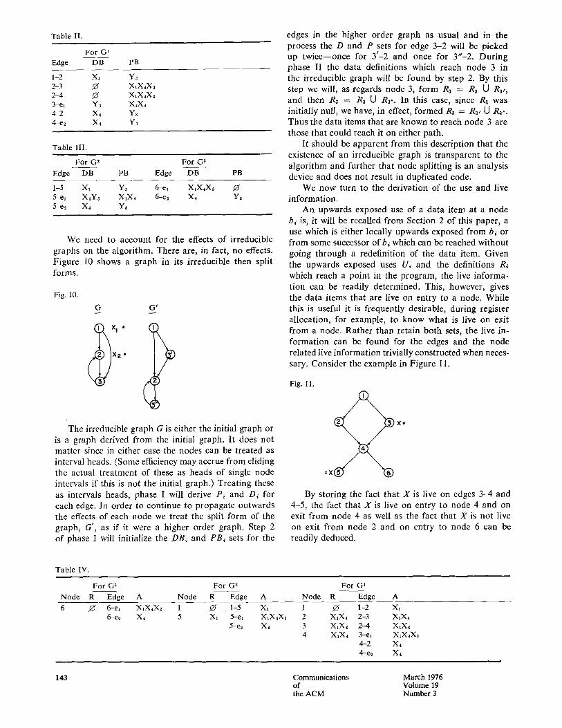
Table II.

For G 1 Edge DB PB

1-2 XI Y3 2-3 Z~ X1X4X3 2-4 Z; XIX4X3 3-e~ Y3 XtX4 4--2 X~ Y3 4--e~ X4 Y~

Table III.

For G 2 For G 3 Edge DB PB Edge DB PB

1-5 Xl Yz 6-et XIX4X3 .~f 5-et X~Y~ XIX4 6-e2 X, Y~ 5-e2 X4 Ya

We need to account for the effects of irreducible graphs on the algorithm. There are, in fact, no effects. Figure 10 shows a graph in its irreducible then split forms.

Fig. 10.

G G'

~ X I •

X 2 •

Fig. 11.

The irreducible graph G is either the initial graph or is a graph derived from the initial graph. It does not matter since in either case the nodes can be treated as interval heads. (Some efficiency may accrue from eliding the actual treatment of these as heads of single node intervals if this is not the initial graph.) Treating these as intervals heads, phase I will derive P~ and D~ for each edge. In order to continue to propagate outwards the effects of each node we treat the split form of the graph, G', as if it were a higher order graph. Step 2 of phase I will initialize the DB~ and PB~ sets for the

edges in the higher order graph as usual and in the process the D and P sets for edge 3-2 will be picked up twice--once for 3 ' -2 and once for 3"-2. During phase II the data definitions which reach node 3 in the irreducible graph will be found by step 2. By this step we will, as regards node 3, form R~ = R~ 13 R~,, and then R3 = R3 U R3.. In this case, since R3 was initially null, we have, in effect, formed R3 = R3, U R3.. Thus the data items that are known to reach node 3 are those that could reach it on either path.

It should be apparent from this description that the existence of an irreducible graph is transparent to the algorithm and further that node splitting is an analysis device and does not result in duplicated code.

We now turn to the derivation of the use and live information.

An upwards exposed use of a data item at a node bi is, it will be recalled from Section 2 of this paper, a use which is either locally upwards exposed from b~ or from some successor of b~ which can be reached without going through a redefinition of the data item. Given the upwards exposed uses Ui and the definitions R~ which reach a point in the program, the live information can be readily determined. This, however, gives the data items that are live on entry to a node. While this is useful it is frequently desirable, during register allocation, for example, to know what is live on exit from a node. Rather than retain both sets, the live information can be found for the edges and the node related live information trivially constructed when neces- sary. Consider the example in Figure 11.

=×

×,

By storing the fact that X is live on edges 3-4 and 4-5, the fact that X is live on entry to node 4 and on exit from node 4 as well as the fact that X is not live on exit from node 2 and on entry to node 6 can be readily deduced.

Table IV.

For G ~ For G 2 Node R Edge A Node R Edge A

For G 1 Node R Edge A

6 .~ 6-el X1X4X3 1 Zf .1-5 6-e~ X4 5 Xl 5-el

5-e~

Xl X1X4X3 X4

1 ~ 1-2 2 XIX4 2-3 3 X1X4 2-4 4 X1X4 3-el

4--2 4-e2

Xl X1X, XIX4 X,X,X3 X, X,

143 Communications of the ACM

March 1976 Volume 19 Number 3

In order to compute the live information for the edges of the graph rather than for the nodes, the set of the definitions, A, available on each edge is used. For a given edge e, incident into node i

L~ = A, fq Ui.

Since A, was derived by the Reach Algorithm, the basic i tem of information which must be derived is U~. The process of determining which uses reach backwards through the graph is analogous to that of determining which definitions reach forwards. Hence to determine what is upwards exposed f rom a node in- volves knowing what is upwards exposed f rom the successors of a node and what data items are preserved through the node.

The algorithm for generating the U~ sets for the nodes of the graph again requires two phases, the first of which can be conveniently imbedded in the first phase of the Reach Algorithm. Given the locally upwards exposed uses f rom each node in the basic graph, the purpose of the first phase is to find the upwards exposed uses f rom each interval and hence the locally upwards exposed uses for each node in the derived graph. The upwards exposed uses f rom each interval is found as follows: 1. Prior to processing each interval initiate a set Uh

which will contain the uses upwards exposed in the interval:

Uh = UBh

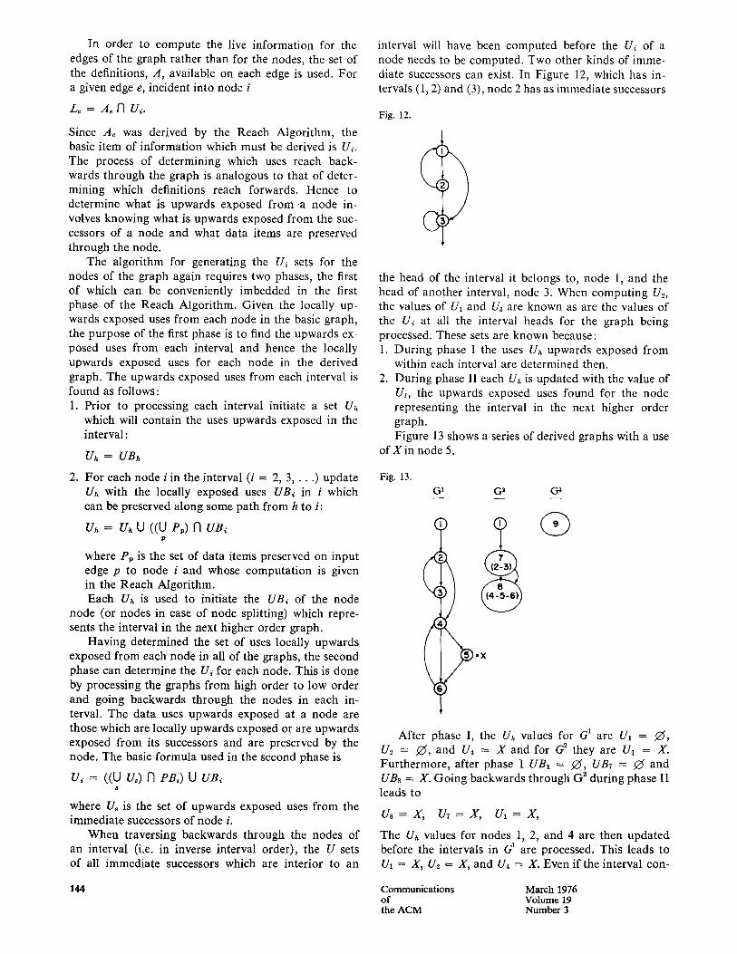
interval will have been computed before the U~ of a node needs to be computed. Two other kinds of immediate successors can exist. In Figure 12, which has intervals (1, 2) and (3), node 2 has as immediate successors

Fig. 12.

(3

the head of the interval it belongs to, node 1, and the head of another interval, node 3. When computing U2, the values of U~ and /-/3 are known as are the values of the U~ at all the interval heads for the graph being processed. These sets are known because: 1. During phase I the uses Uh upwards exposed f rom

within each interval are determined then. 2. During phase II each Uh is updated with the value of

Uz, the upwards exposed uses found for the node representing the interval in the next higher order graph. Figure 13 shows a series of derived graphs with a use

of X in node 5.

2. For each node i in the interval (i --- 2, 3 , . . . ) update Uh with the locally exposed uses UB~ in i which can be preserved along some path f rom h to i:

Uh = Uh U ((U P,) 17 UB~ p

where P, is the set of data items preserved on input edge p to node i and whose computat ion is given in the Reach Algorithm. Each Uh is used to initiate the UB~ of the node

node (or nodes in case of node splitting) which represents the interval in the next higher order graph.

Having determined the set of uses locally upwards exposed f rom each node in all of the graphs, the second phase can determine the U~ for each node. This is done by processing the graphs f rom high order to low order and going backwards through the nodes in each interval. The data uses upwards exposed at a node are those which are locally upwards exposed or are upwards exposed f rom its successors and are preserved by the node. The basic formula used in the second phase is

U, = ((U U.) n PB,) U UB, $

where U. is the set of upwards exposed uses f rom the immediate successors of node i.

When traversing backwards through the nodes of an interval (i.e. in inverse interval order), the U sets of all immediate successors which are interior to an

Fig. 13. G 1 G 2 G 3

After phase I, the Uh values for G 1 are U1 = .(Zf, U2 = .~, and U4 = X and for G 2 they are U1 = X. Furthermore, after phase I UB1 = J25, UBv = Zf and UB8 ~- X. Going backwards through G 2 during phase I I leads to

Us=X, UT=X, UI=X,

The Uh values for nodes 1, 2, and 4 are then updated before the intervals in G 1 are processed. This leads to U1 = X, U2 = X, and U4 -- X. Even if the interval c o n -


sisting of (2, 3) is processed before (4, 5, 6), the U~ for the two successors of node 3 are known since U: = X and U4 = X have already been established.

As has already been observed, phase I of the live analysis algorithm can be embedded in phase I of the Reach Algorithm. Since the second phase of the live algorithm requires a backwards pass through the graph it cannot be embedded in phase II of the Reach Al- gorithm. The combined algorithm therefore requires three phases. We will not give any more details on this in algorithmic form since the procedure in the next section gives a more definitive version of the combined data flow analysis.

6. A Data Flow Analysis Procedure

A P L / I program, DATFLOW, which finds the definitions that reach each node, the uses that are upwards exposed from a node and its successors, and the definitions that are live on each edge of the control flow graph is given in this section. Before giving the procedure, two representational techniques which greatly affect the actual speed of the algorithm are described. We first describe the representation of the data sets and then the representation of the control flow information.

Associated with each node i on input to the procedure is the set of uses, UB~, which are locally upwards exposed from the node; associated with each edge e are the DBe and PB, sets. DB, contains the data definitions defined in the node and available on the exit edge e. PB, contains the data definitions in the program which may be preserved through the node when exit edge e is taken. The operations on these sets and on others formed by the analysis are almost entirely intersection and union. By expressing the sets as comparable bit vectors, the more rapid boolean operations of and and or can be used.

Each bit in the vectors represents a definition in the program. A correspondence table is used to correlate the bit vector entry with the definition point: the ith bit in a bit vector corresponds to the ith entry in the correspondence table where the program location of the definition is recorded.

An obvious question arises: how are the UB and U sets encoded so that they can be meaningfully intersected with the vectors of available definitions? A use of a data item is multiply encoded: if X is the data item being used then that use is encoded by using all the bit entries for definitions of X. Figure 14 shows the DB, PB, and UB vectors for the three nodes and four edges.

We now turn to the representation of the control flow. The nodes of the graphs have been arbitrarily numbered from l to n with all the nodes in a given graph having a contiguous sequence of numbers which is larger than those of the next lower order graph. These numbers are used to uniquely identify the node and in the D A T F L O W procedure to index any data associated

Fig. 14.

Correspondence X ~ ( Table Y

I Entry Def

1 X~ X •

2 Y~ 3 3 Xz 4 X3 -X (~

X,

DBI = 1100

PB~ = 0000 DB2 = 1100

2 PB~ = 0000

DBa = 0010

PB3 = 0100 D B ~ = 0 0 0 1

PB~ = 0100

UBt = 0000 UB~ = 0000

UB~ = 1011

with it. The edges are similarly though independently numbered from 1 to m. A table, GRAPHS, has an entry for each graph which gives the first and last node and the first and last edge in the graph. The table is ordered by graph level with the initial (low order) graph as the first entry.

Associated with the graphs is a node ordered edge listing (called EDGES TABLE in the program). It has the following characteristics: 1. Every edge in the graph appears in the table twice:

once as the in-edge of a node and once as an out- edge.

2. All of the edges incident to a node are given in se- quential entries with all in-edges appearing before all out-edges.

3. E a c h entry contains the node index and the edge index as well as indicators to indicate whether or not the node is an interval header, whether the edge is an in-edge or an out-edge and if an out-edge whether or not it is a latch (is an in-edge to the head of the interval containing it).

4. The interval process order on the nodes is used to determine the order of the entries in the table. All entries for an interval are grouped together with the entries for the header node first. The order of entries for the different intervals in a given graph is not important for the procedure. Kennedy [16] has recently proposed a node listing

approach to data flow analysis which is of 0(l) where l is the length of the list. Aho and Ullman [2] have given an algorithm for producing such a listing for reducible graphs. In their algorithm a listing whose length is O(n log n) can be found for a reducible graph of n nodes. Furthermore if the number of edges is of O(n), then the listing can be found in O(n log n) time. Since the procedure given here associates information with both edges and nodes it is roughly 0(l' .q- n') where l' is the number of entries in EDGES TABLE and n' is the number of nodes in the collection of graphs.

Figure 15 shows the entries for the first order graphs; the entries for the second order would follow.

Processing a graph in a phase of the algorithm in- volves making a pass through the EDGES T A B L E - - forwards for the phases that compute reaching information and backwards for the second phase of the live computation (phase III in the procedure). The node and edge fields index the tables where the information is


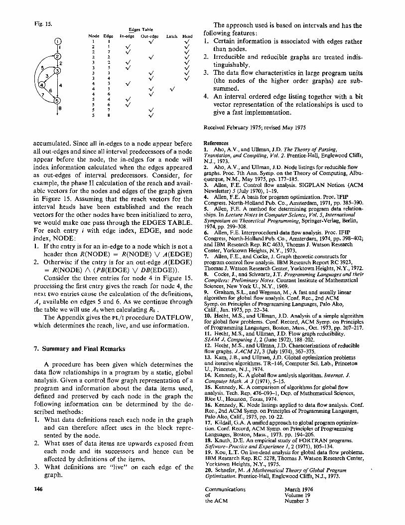
Fig. 15.

)

4

Edges Table Node Edge In-edge Out-edge Latch Head

l l x / x / 2 I "V / V t 2 7 %/ %/ 2 2 %,/ %/ 3 2 x/ x/ 3 5 V X/' 3 3 "V / X/ 3 4 X/ X/ 4 3 x / 4 5 x/ 4 6 ~/ 5 4 5 6 x/ 5 7 x/ 5 s x/

accumulated. Since all in-edges to a node appear before all out-edges and since all interval predecessors of a node appear before the node, the in-edges for a node will index information calculated when the edges appeared as out-edges of interval predecessors. Consider, for example, the phase II calculation of the reach and available vectors for the nodes and edges of the graph given in Figure 15. Assuming that the reach vectors for the interval heads have been established and the reach vectors for the other nodes have been initialized to zero, we would make one pass through the EDGES TABLE. For each entry i with edge index, EDGE, and node index, N O D E : 1. If the entry is for an in-edge to a node which is not a

header then R(NODE) = R(NODE) ~/ A(EDGE) 2. Otherwise if the entry is for an out-edge A(EDGE)

= R(NODE) /~ (PB(EDGE) V DB(EDGE)). Consider the three entries for node 4 in Figure 15.

processing the first entry gives the reach for node 4, the next two entries cause the calculation of the definitions, A, available on edges 5 and 6. As we continue through the table we will use A6 when calculating R~.

The Appendix gives the PL/I procedure DATFLOW, which determines the reach, live, and use information.

7. S u m m a r y and F i n a l R e m a r k s

A procedure has been given which determines the data flow relationships in a program by a static, global analysis. Given a control flow graph representation of a program and information about the data items used, defined and preserved by each node in the graph the following information can be determined by the described methods: 1. What data definitions reach each node in the graph

and can therefore affect uses in the block represented by the node.

2. What uses of data items are upwards exposed from each node and its successors and hence can be affected by definitions of the items.

3. What definitions are "live" on each edge of the graph.

146

The approach used is based on intervals and has the following features: 1. Certain information is associated with edges rather

than nodes. 2. Irreducible and reducible graphs are treated indis-

tinguishably. 3. The data flow characteristics in large program units

(the nodes of the higher order graphs) are sub- summed.

4. An interval ordered edge listing together with a bit vector representation of the relationships is used to give a fast implementation.

Received February 1975; revised May 1975

References 1. Aho, A.V., and Ullman, J.D. The Theory of Parsing, Translation, and Compiling, Vol. 2. Prentice-Hall, Englewood Cliffs, N.J., 1973. 2. Aho, A.V., and Ullman, J.D. Node listings for reducible flow graphs. Proc. 7th Ann. Syrup. on the Theory of Computing, Albu- querque, N.M., May 1975, pp. 177-185. 3. Allen, F.E. Control flow analysis. SIGPLAN Notices (ACM Newsletter) 5 (July 1970), 1-19. 4. Allen, F.E. A basis for program optimization. Proc. IFIP Congress. North-Holland Pub. Co., Amsterdam, 1971, pp. 385-390. 5. Allen, F.E. A method for determining program data relationships. In Lecture Notes in Computer Science, Vol. 5, International Symposium on Theoretical Programming, Springer-Verlag, Berlin, 1974, pp. 299-308. 6. Allen, F.E. Interprocedural data flow analysis. Proc. IFIP Congress, North-Holland Pub. Co., Amsterdam, 1974, pp. 398-402; and IBM Research Rep. RC 4633, Thomas J. Watson Research Center, Yorktown Heights, N.Y., 1973. 7. Allen, F.E., and Cocke, J. Graph theoretic constructs for program control flow analysis. IBM Research Report RC 3923, Thomas J. Watson Research Center, Yorktown Heights, N.Y., 1972. 8. Cocke, J., and Schwartz, J.T. Programming Languages and their Compilers: Preliminary Notes. Courant Institute of Mathematical Sciences, New York U., N.Y., 1969. 9. Graham, S.U, and Wegman, M.,A fast and usually linear algorithm for global flow analysis. Conf. Rec., 2nd ACM Symp. on Principles of Programming Languages, Palo Alto, Calif., Jan. 1975, pp. 22-34. 10. Hecht, M.S., and Ullman, J.D. Analysis of a simple algorithm for global flow problems. Conf. Record, ACM Symp. on Principles of Programming Languages, Boston, Mass., Oct. 1973, pp. 207-217. 11. Hecht, M.S., and Ullman, J.D. Flow graph reducibility. SIAM J. Computing 1, 2 (June 1972), 188-202. 12. Hecht, M.S., and Ullman, J.D. Characterizations of reducible flow graphs. J.ACM21, 3 (July 1974), 367-375. 13. Kam, J.B., and Ullman, J.D. Global optimization problems and iterative algorithms. TR-146, Computer Sci. Lab., Princeton U., Princeton, N.J., 1974. 14. Kennedy, K. A global flow analysis algorithm. Internat. J. Computer Math. A 3 (1971), 5-15. 15. Kennedy, K. A comparison of algorithms for global flow analysis. Tech. Rep. 476-093-1, Dep. of Mathematical Sciences, Rice U., Houston, Texas, 1974. 16. Kennedy, K. Node listings applied to data flow analysis. Conf. Rec., 2nd ACM Symp. on Principles of Programming Languages, Palo Alto, Calif., 1975, pp. 10-22. 17. Kildall, G.A. A unified approach to global program optimization. Conf. Record, ACM Syrup. on Principles of Programming Languages, Boston, Mass., 1973. pp. 194-206. 18. Knuth, D.E. An empirical study of FORTRAN programs. Software-Practice and Experience 1, 2 (1971), 105-134. 19. Kou, L.T. On live-dead analysis for global data flow problems. IBM Research Rep. RC 5278, Thomas J. Watson Research Center, Yorktown Heights, N.Y., 1975. 20. Schaefer, M. A Mathematical Theory of Global Program Optimization. Prentice-Hall, Englewood Cliffs, N.J., 1973.


Appendix. The P L / I Procedure D A T F L O W

* * * * * * * * * * * * * * * * * * * * * * * * * * GATF LO~; * * * * * * * * * * * * * * * * * * * * * * * * * * * * * * * * * * / * DATFLOW DETERMINES TIIE DATA DEFINITIONS TIIAT REAC',I EACM NODE FROM * / / * PREDECESSOR NODES, THE USES TIIAT ARE UPWARDS EXPOSED AT A NODE *I / * FROM BDTil TIIE NODE AND FROM SUCCESSOR NODES, ANFI THE DATA */ / * DEFINITIONS TIIAT ARE ALIVE ALONG EAC!t EDGE. THIS INFOR~ATIDN * / / * IS EXPRESSED IN TIlE REACII, USED AND LIVE VECTC)RS RESPECTIVELY. * I / * DATELOW INPUT IS A DESCRIPTION OF THE PROGRAm4 COrlTROL FLDI; * / / * RELATIONSHIPS, AND LOCAL INFORMATION ABOUT THE DATA ITEMS USED, * / 1, DEFINED AND PRESERVED ON TIIE NODES AND EDGES OF THE GRAPH. ,1 / * TIIE PROGNAr~ CONTROL FLOW RELATIONSHIPS ARE GIVEN IN SNAP';S, * / / * EDGES_TABLE, FROM_TO_TABLE, CORRES_tIEAD, AND GORGES_EDGE. * / / * T!IESE RELATIONSHIPS ARE DETERMINED BY TIIE INTERVAL ANALYZER. * / /* TIIE LOCAL INFORMATION AROUT TIIE DATA ITEMS IS GIVEN IN "1 / * EDGEDATA AND IN NODEDATA. * / 1 . GRAPtlS CONTAINS ONE ENTRY FOR EAC!I GRAPH (BASIC, DERIVED, OR * / / * S P L I T ) . EASlt ENTRY CONTAINS INDICES FOR TIlE FIRST AND LAST NOnE * / / * AND TIlE FIRST AND LAST EDGE. * / / * EDGESTABLE CONTAINS 2 ENTRIES FOR EACII EDGE IH TIIE GRAPHS. * / / * TIIE TABLE IS ORDERED SO THAT ALL NODES IN AN INTERVAL ARE IN TIIE*/ / * TABLE IN INTERVAL ORDER. FURTHER ALL TIIE ENTRIES FOR EDGES * / / * ENTERING A NODE IMMEDIATELY PRECEDE THE EXIT EDGES. ALL NODES * / / * FOR A GRAPH ARE GROUPED. THE TABLE ORDER IS USED AS THE ORPER * / / * FOR PROCESSING THE INFORMATION. * / / * FROM_TOTABLE CONTAINS 2 ENTRIES FOR EACH EDGE IN THE GRAPNS: * / /* TIIE NODE TIIE EDGE COMES FROM AND TIlE NODE IT ENTERS. *I I - CORRES MEAD CONTAINS AN ENTRY FOR EACH NODE IN THE IIIGHER ORDER * / / * GRAPHS: TIIE IIEAD OF TIrE INTERVAL WHICM THIS NODE REPRESENTS. * / / * IF TIlE GRAPH IS THE RESULT OF SPLITTING TItEN MORE TITAN ONE NODE * / / * MAY INDEX TIlE SAME NODE IN TIlE NEXT LOV;ER ORDER GRAPH. "1 / * T i l lS TABLE IS USED WIIEN NODE RELATED INFORMATION IS POSTED UP * / / * (DURING PIIASE I ) OR DONN (DURING PHASE I I ) , * / / * CORRES_EDGE CONTAINS AN ENTRY FOR EACH EDGE IN THE HIGHER ORDER " / /¢ GRAPHS: TIIE EDGE IN THE NEXT LOWER ORDER GRAPH WHICH THIS EDGE * / / " REPRESENTS. IF TIIE GRAPH IS TIIE RESULT OF SPLITTINC TIIEN MORE */ / * TIIAN ONE EDGE MAY INDEX TIlE SAItE EDGE IN THE NEXT LOitER GRAPH. * / 1 . T i l lS TABLE IS USED WIIEN EDGE RELATED INFORMATION IN POSTED UP *'/ /, (DURING PltASE I ) OR DONN (DURING PtlASE I I ) , * / 1. EDGE_DATA CONTAINS TIIE EDGE RELATED LOCAL INFORMATION: * / / * DB ARE TIlE DEFINITIONS IN THE NODE WIIICH ARE AVAILABLE ON EXIT * / I* PB ARE TIIE DEFINITIONS IN TIIE PROGRAM ~/tllC'l ARE PRESERVED qY 4/ / * TIIE NODE. ON ENTRY TO DATFLOI; TIIE DB AND Pq FOR ONLY * / / * BASIC NODES IS GIVEN. DATFLOW DETERMINES On AN D Pq FOR THE -1 / * NODES OF THE IIIGllER ORDER GRAPHS. "1 I * NODE_DATA CONTAINS THE NODE RELATED LOCAL INFORMATION: .1 / * US ARE TIIE USES IN THE NODE WIIICH ARE UPUARDS EXPOSED. ON ENTRY * I 1 . TO DATFLOW TIlE UB FOR BASIC NODES ARE GIVEN. DATFLO'I DETERrIINES * / 1. THE UB FOR TIIE NODES OF TIIE IIISIIER ORDER GRAPHS. * / * * * * * * * * * * * * * * * * * * * * * * * * * * * * * * * * * * * * * * * * * * * * * * * * * * * * * * * * * * * * * * * * * * * * * * *

DATFLU~;:PNDC(URAPiIS, EDGES_TABLE,FROFI_TO_TADLE,CORRES_HEAD,CORRES_EDGE, EDGE_DATA, NODE_DATA, REACH, US ED, L I VE ) ;

DCL I GRAPIIS (NO OF GRAPHS) CTL, /*FOR EACH GRAPH: * / 2 FIRST_NGDE FIXED DIN(15), /*INDX OF IST NODE * / 2 LAST_NUDE FIXED BIN(15), /*INDX OF LAST NODE * / 2 FIRST EDGE FIXED BIN(15), /*INDX OF 1ST EDGE * / 2 LAST_EDGE FIXED BIN(15); /*INDX OF LAST EDGE * /

DCL I EDGES_TABLE (2*NO_OF_EDGES) CTL, / *2 ENTRIES FOR EACII EDGE IN*/ 2 INDICATORS, /*GRAPHS. * I

3 IN EDGE B I T ( l ) , /*ON IF EDGE ENTERS NODE * / 30U~_EDDE R I T ( 1 ) , /*ON IF EDGE LEAVES NODE * / 3 LATCH B I T ( l ) , /*ON IF OUT EDGE ArID LATCH * / 3 IIEADER B I T ( l ) , /*ON IF NODE IS AN INT HEAD * I

2 NODE FIXED BIN(1S), /*INDX TO NODE RELATED INED * / 2 EDGE FIXED B I N ( 1 5 ) ; /41RDX TO EDGE RELATED INFO -1

DCL 1 FSDtt TO TABLE(NO_OFEDGES) CTL, /*FOR EACH EDGE: * / 2 FROM FIXED B I N ( 1 5 ) , / * THE NODE IT COMES EROIA * / 2 TO FIXED B I N ( 1 5 ) ;

DCL CORRES_IIEAD (NO_OF_NODES) CTL FIXED BIN(15);

DCL CORRES_EDGE (NO_OF_EDGES) CTL FIXED B I N ( 1 5 ) ;

/ * THE NODE IT GOES TO * I

/*FOR EACH NODE--THE HEAD OF*/ /.THE INTERVAL IVIIICM THIS * / /*NODE REPRESENTS * /

/4FOR EACH EDGE; EDGE IN TI tE* / /*NEXT LOWER ORDER GRAPH IT * / /*CORRESPONDS TD . /

DCL 1 EDGE DATA (NO OF_EDGES) CTL, 2 D B - - BIT(NO_OF_DEFS), 2 PB BIT(NO_OF_DEFS);

DCL L NODE_DATA (NO_OF_NODES) CTL, 2 UB DIT(NOOF_DEFS);

/ * * * * DECLARATIONS OF OUTPUT DATA

DCL USED.(NO_OF_NODES) BIT(NO OF_DEFS) CTL; DCL REACII(NO OF NODES) BIT(NO~OF_DEFS) CTL; BCL LIVE (NO_OF_EDGES) BIT(NO_OF_BEES) CTL;

/ * * * * DECLARATIONS OF LOCAL ~ATA

DCL NO OF GRAPIIS FIXED B I N ( 1 5 ) ; NCL NO_OF_NODES FIXED B I N ( 1 5 ) ; DCL NO_OF_EDGES FIXED BIN(IS) ; DCL NO_OF_DEFS FIXED B I N ( 1 5 ) ; DCL IIEAO FIXED B I N ( 1 5 ) ; GEL G FIXED R I N ( E 5 ) ; OCL I FIXED B I N ( 1 5 ) ;

4 * * * /

* * * * /

/ * * * * * * * * * * * * * * * * * * * START OF pROGRA~.I * * * * * * * * * * * * * * * * * * * * * * * * * * * * * NO_OFGBAPHS=DItI(GRAP'IS.FIRST_NODE, 1 ) ; NO_OFNODES=UIM(NODEDATA.UD,1); NO_OF_EDGES=DIt4(EDGEDATA.DB, I ) ; NO_OFDEFS=LENGTtI(DB(1)); ALLOCATE REACH INIT((NO_OF_NODES)IOIB); ALLOCATE USED; USED=UB; / * IN IT . USED TO UB FOR BASIC NUDES AND TD n FOR ALL OTHERS*/

/ * * . 4 4 4 , * * * PItASE I - LOW ORDER GRAPH TO HIGH ORDER SRAPIt * * * * * * * * * * * / BEGINt DCL P (NO OF_EDGES) BIT(NO_OF_DEFS); /*PRESERVED OH PATII * / DCL D (NO_OF_EDGES) RIT(NO_OF_DEES); /*DEFINED ON PATH * / DCL Pi t ; (NO_OFNODES) BIT(NO_OF_BEES) /*PRESERVED ON ENTRY*/

INIT((NO_OF_NODES)'D'R); DCL DIN (NO_OF_NODES) BIT(ND_OE_DEFS) /*~EEIRED ON ENTRY*/

INIT((NO_OE_NODES)'g'B); DO G=l TO NO_OF_GRAPIISol;

IF G>l THEN DO; / * PICK UP DATA FROM LOI~ER GRAPH * /

DO I=EIRST EDGE(G) TO LASTEDGE(G); PB(1)=PTCORRES_EDGE(1)); DB(I)=REACH(CORRES_HEAD(FROM(I))) & PD( I ) I

D(CORRES_EDGE(I)) ; END; DO 1=FIRST NODE(G) TO LAST NODE(G);

UB(1)=U~ED(CORRES_HEAD(1)); REACII(1)=NEACH(CORRES_HEAD(1));

END; END;

HEAD=B; DO I=2*FIRST_EDGE(G)-I TO 2*LAST_EDGE(G);

IF IIEADER(1) THEN DO;

IF IIEAD "= NODE(1) TMEN HEAD=NODE(1); IF OUT EDGE(I)

~HEN DO; P (EDGE(1 ) )=PB(EDGE(1 ) ) ; D ( E D G E ( I ) ) = D R ( E D G E ( I ) ) ;

END; END; ELSE / * NOT A HEADER NODE * /

IF IN EDGE(I) TH~N DO;

P I N ( N O D E ( I ) ) = P I N ( N O D E ( I ) ) I P l E D G E ( I ) ) ; D I N ( N O D E ( I ) ) = D I N ( N O D E ( I ) ) I D ( E D O E ( I ) ) ; USED(HEAD)=USED(t tEAD)I(P(EDGE(I) ) & U D ( N O D E ( I ) ) ) ;

END; ELSE DO; / * FOR THE OUT EDGE * /

P(EDGE(1))=PIN(NODE(1)) & PR(EDGE(1)); D(EDGE(1))=DIN(NODE(1)) & PB(EDGE(1)) IDR(EOGE(1));

END; IF LATCl t ( I ) THEN REACII(MEAD)=REACH(tlEAD) I D ( E D G E ( I ) ) ;

END; 1- OF PROCESSING A GRAPH * / END; / * OF pROCESSING ALL GRAPHS BY PHASE I * / END; / * OF BEGIN BLOCK (LOCAL DATA IS FREED) * /

/ * * * * * * * * * * * * * * * * * * * THE END OF PHASE I * * * * * * * * * * * * * * * * * * * * * * * * * * * * * * *

/ * * * * * * * PIIASE I I - PROCESS GRAPHS FROM IIIGH ORDER TO LOW ORDER * * . 4 . * / BEGIN;

DCL A (NO OF EDGES) BIT(NO OF DEFS) IN IT ( (NO OF EDGES) '01R) ; REACH(NO_0F_NO~ES'~=I0'B; /*INITTALTZE TO DEFS THAT R-EACII PROGRAM 4/ DO G=NO_OF_GNAPHS-I TO ]. BY - 1 ;

DO I=FIRST NODE(G*1) TO LAST_NODE(G*I); REACH(COGBES_IIEAD(1))=REACH(CORRES_IIEAD(1)) I REACII(1);

END; DO 1=2*FIRST_EDGE(G)- I TO 2*LAST_EDGE(G);

I F I N_EDGE( I ) & ~HEADER( I ) THEN REACH(NODE(I))=REACH(NOOE(1)) I A ( E D S E ( I ) ) ;

IF OUT_EDGE(b) TIIEN A(EDGE( I ) )=REACH(NODE( I ) ) & PD(EDGE( I ) ) I

DB( EDGE( I ) ) ; END; / * OF PROCESSING GRAPIt * /

END; / * OF PROCESSING ALL GRAPHS By PItASE I I * / / * * * * * * * * * * * * * * * * * TIlE END OF PHASE I I * * * * * * * * * * * * * * * * * * * * * * * * * * * * * * * *

/ * * * * * * * * * * * * * * * * PIIASE I I I - LIVE ANALYSIS * * * * * * * * * * * * * * * * * * * * * * * * * * * ALLOCATE LIVE; USED ( NO_OF_NODES ) =USED ( CORR ES_HEAD (NO_OF_NODES) ) ; UB (NO OF_NOD ES ) =USED ( CORR ES_ftEAD ( NO_OF_NODES ) ) ; DO G=NO_OF_GRAP!IS-I TO 1 BY - I ;

DO I :F IRST NODE(G*I) TO LAST_NODE(G+1); USED(CORNES_IIEAD(1)):USED(CORRES_IIEAD(1)) I U B ( 1 ) ;

END; DO 1=2*LAST_EDGE(G) TO 2*FIRST_EDGE(G)-E BY - 1 ;

IF OUT EDGE(I) & " I IEADER(I ) THEN USED( NODE( I ) ) =USED( NODE( I ) ) I (USED( TO( EDGE( I ) ) )DPB (EDGE( I ) ) ) ;

IF IN EDGE(I) TIIEN L I V E ( E D G E ( I ) ) : U S E D ( N O D E ( I ) ) & A ( E D G E ( I ) ) ;

El;O; / * OF PROCESSING GRAPH * / END; / * OF LIVE ANALYSIS " / END; / * OF BEGIN BLOCK * / RETURN;

END; / * * * * * * * * * * * * * * * * * * * * * * * N O OF GATFLOW * * * * * * * * * * * * * * * * * 4 4 * * * * * 4 4 * * * * * *

147 Communications March 1:976 of Volume 19 the ACM Number 3

a program data flow analysis procedure - turing award · programming techniques g. manacher, s....

Documents