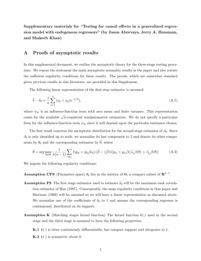
Supplementary materials for “Testing for causal effects in a generalized regres-

sion model with endogenous regressors” (by Jason Abrevaya, Jerry A. Hausman,

and Shakeeb Khan)

A Proofs of asymptotic results

In this supplemental document, we outline the asymptotic theory for the three-stage testing proce-

dure. We repeat the statement the main asymptotic-normality results in the paper and also restate

the sufficient regularity conditions for these results. The proofs, which are somewhat standard

given previous results in this literature, are provided in this Supplement.

The following linear representation of the first-step estimator is assumed:

δ − δ0 =1n

n∑i=1

ψδi + op(n−1/2), (A.1)

where ψδi is an influence-function term with zero mean and finite variance. This representation

exists for the available√n-consistent semiparametric estimators. We do not specify a particular

form for the influence-function term ψδi since it will depend upon the particular estimator chosen.

The first result concerns the asymptotic distribution for the second-stage estimator of β0. Since

β0 is only identified up to scale, we normalize its last component to 1 and denote its other compo-

nents by θ0 and the corresponding estimator by θ, where

θ = arg maxθ∈Θ

1n(n− 1)

∑i 6=j

1[y2i = y2j ]kh(z′iδ − z′j δ)1[y1i > y1j ]1[z′1iβ(θ) > z′1jβ(θ)] (A.2)

We impose the following regularity conditions:

Assumption CPS (Parameter space) θ0 lies in the interior of Θ, a compact subset of Rk−1.

Assumption FS The first stage estimator used to estimate δ0 will be the maximum rank correla-

tion estimator of Han (1987). Consequently, the same regularity conditions in that paper and

Sherman (1993) will be assumed so we will have a linear representation as discussed above.

We normalize one of the coefficients of δ0 to 1 and assume the corresponding regressor is

continuously distributed on its support.

Assumption K (Matching stages kernel function) The kernel function k(·) used in the second

stage and the third stage is assumed to have the following properties:

K.1 k(·) is twice continuously differentiable, has compact support and integrates to 1.

K.2 k(·) is symmetric about 0.

1

K.3 k(·) is a pth order kernel, where p is an even integer:∫ulk(u)du = 0 for l = 1, 2, ...p− 1∫upk(u)du 6= 0

Assumption H (Matching stages bandwidth sequence) The bandwidth sequence hn used in the

second stage and the third stage satisfies√nhpn → 0 and

√nh3

n →∞.

Assumption RD (Last regressor and index properties) z(k)1i is continuously distributed with pos-

itive density on the real line conditional on z′iδ0 and all other elements of z1i. Moreover, z′iδ0

is nondegenerate conditional on z′1iβ0.

Assumption ED (Error distribution) (εi, ηi) is distributed independently of zi and is continuously

distributed with positive density on R2.

Assumption FR (Full rank condition) Conditional on (z′iδ0, y2i), the support of z1i does not lie

in a proper linear subspace of Rk.

The following lemma establishes the asymptotic properties of the second stage estimator of θ0.

Some additional notation is used in the statement of the lemma. The reduced-form linear index is

denoted ζδi = z′iδ0 and fζδ() denotes its density function. FZ1 denotes the distribution function of

z1i. Also, ∇θθ denotes the second-derivative operator.

Lemma 1 If Assumptions CPS, FS, K, H, RD, ED, and FR hold, then

√n(θ − θ0)⇒ N(0, V −1ΩV −1) (A.3)

or, alternatively, θ − θ0 has the linear representation

θ − θ0 =1n

n∑i=1

ψβi + op(n−1/2) (A.4)

with V = ∇θθN (θ) |θ=θ0 and Ω = E[δ1iδ′1i], and ψβi = V −1δ1i, where

N (θ) =∫

1[z′1iβ(θ) > z′1jβ(θ)]H(ζj , ζj)F(z′1iβ0, z′1jβ0, ζj , ζj)dFZ1,ζ(z1i, ζj)dFZ1,ζ(z1j , ζj) (A.5)

with ζi = z′iδ0, whose density function is denoted by fζ , and where

F(z′1iβ0, z′1jβ0, ζi, ζj) = P (y1i > y1j |y2i = y2j , z1i, z1j , ζi, ζj) (A.6)

H(ζi, ζj) = P (y2i = y2j |ζi, ζj) (A.7)

and the mean-zero vector δ1i is given by

δ1i =(∫

fζ(ζi)µ31(ζi, ζi, β0)dζi

)ψδi (A.8)

2

where

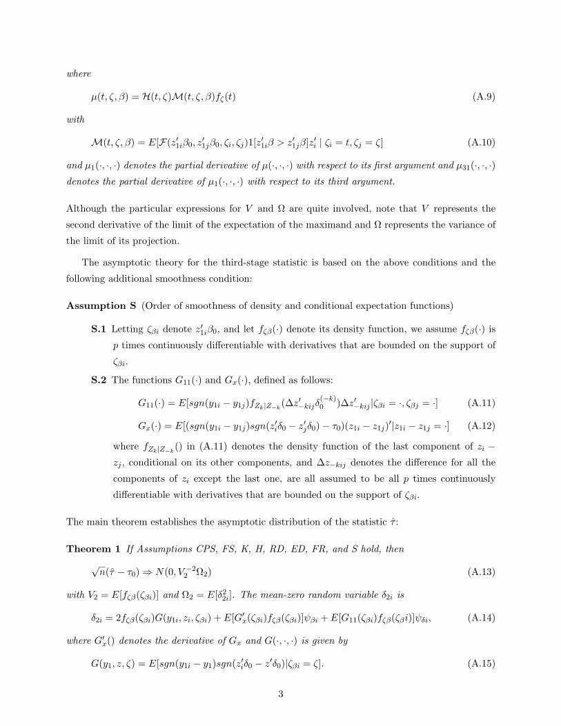
µ(t, ζ, β) = H(t, ζ)M(t, ζ, β)fζ(t) (A.9)

with

M(t, ζ, β) = E[F(z′1iβ0, z′1jβ0, ζi, ζj)1[z′1iβ > z′1jβ]z′i | ζi = t, ζj = ζ] (A.10)

and µ1(·, ·, ·) denotes the partial derivative of µ(·, ·, ·) with respect to its first argument and µ31(·, ·, ·)denotes the partial derivative of µ1(·, ·, ·) with respect to its third argument.

Although the particular expressions for V and Ω are quite involved, note that V represents the

second derivative of the limit of the expectation of the maximand and Ω represents the variance of

the limit of its projection.

The asymptotic theory for the third-stage statistic is based on the above conditions and the

following additional smoothness condition:

Assumption S (Order of smoothness of density and conditional expectation functions)

S.1 Letting ζβi denote z′1iβ0, and let fζβ(·) denote its density function, we assume fζβ(·) is

p times continuously differentiable with derivatives that are bounded on the support of

ζβi.

S.2 The functions G11(·) and Gx(·), defined as follows:

G11(·) = E[sgn(y1i − y1j)fZk|Z−k(∆z′−kijδ

(−k)0 )∆z′−kij |ζβi = ·, ζβj = ·] (A.11)

Gx(·) = E[(sgn(y1i − y1j)sgn(z′iδ0 − z′jδ0)− τ0)(z1i − z1j)′|z1i − z1j = ·] (A.12)

where fZk|Z−k() in (A.11) denotes the density function of the last component of zi −

zj , conditional on its other components, and ∆z−kij denotes the difference for all the

components of zi except the last one, are all assumed to be all p times continuously

differentiable with derivatives that are bounded on the support of ζβi.

The main theorem establishes the asymptotic distribution of the statistic τ :

Theorem 1 If Assumptions CPS, FS, K, H, RD, ED, FR, and S hold, then√n(τ − τ0)⇒ N(0, V −2

2 Ω2) (A.13)

with V2 = E[fζβ(ζβi)] and Ω2 = E[δ22i]. The mean-zero random variable δ2i is

δ2i = 2fζβ(ζβi)G(y1i, zi, ζβi) + E[G′x(ζβi)fζβ(ζβi)]ψβi + E[G11(ζβi)fζβ(ζβi)]ψδi, (A.14)

where G′x() denotes the derivative of Gx and G(·, ·, ·) is given by

G(y1, z, ζ) = E[sgn(y1i − y1)sgn(z′iδ0 − z′δ0)|ζβi = ζ]. (A.15)

3

A.1 Proof of Lemma 1

The proof strategy will be along the lines of Sherman (1994), and we deliberately aim to keep

notation as similar as possible to that used in that paper. Specifically, let Gn(θ) and Gn(θ) be

defined as1

Gn(θ) =1

n(n− 1)

∑i 6=j

1[y2i = y2j ]kh(z′iδ0 − z′jδ0)1[y1i > y1j ]1[z′1iβ(θ) > z′1jβ(θ)] (A.16)

Gn(θ) =1

n(n− 1)

∑i 6=j

1[y2i = y2j ]kh(z′iδ − z′j δ)1[y1i > y2j ]1[z′1iβ(θ) > z′1jβ(θ)] (A.17)

Similar to Sherman (1994), the proof strategy involves the following stages:

1. Establish consistency of the estimator.

2. Show the estimator converges at the parametric (√n) rate.

3. Establish asymptotic normality of the estimator.

For consistency, we apply Theorem 2.1 in Newey and McFadden (1994). Compactness follows

from Assumption CPS. To show uniform convergence, we note that the estimated first-stage index

converges uniformly to the true index, by Assumption FS, so we can replace estimated indexes with

true values inside the objective function, and work with Gn(θ). Next, we note by Theorem 2 in

Sherman (1994),

supθ∈Θ

(Gn(θ)− E[Gn(θ)]) = op(1) (A.18)

by the Euclidean property of the indicator function 1[z′1iβ > z′1jβ], and the uniform (in n) bound-

edness of E[Gn(θ)]. By a change of variables and Assumptions K and H,

supθ∈Θ

E[Gn(θ)]− G(θ)p→ 0 (A.19)

where we will define G(θ) as follows. First, define the indicator dij as 1[y2i = y2j ], and define

H(z′iδ0, z′jδ0) = E[dij |z′iδ0, z

′jδ0].

Furthermore, define

F(z′1iβ0, z′1jβ0, z

′iδ0, z

′jδ0) = P (y1i > y1j |dij = 1, z′1iβ0, z

′1jβ0, z

′iδ0, z

′jδ0).

1Implicit in the proofs that follow, we are subtracting the function 1[z′1iβ0 > z′1jβ0] from 1[z′1iβ(θ) > z′1jβ(θ)] in

each of the two objective functions, analogous to Sherman (1993). The terms subtracted do not affect the value of

the estimator, and are omitted for notational convenience.

4

So we can define

G(θ) = E[F(z′1iβ0, z′1jβ0, z

′iδ0, z

′iδ0)H(z′iδ0, z

′iδ0)1[z′1iβ(θ) > z′1jβ(θ)]] (A.20)

where the above expectation is taken with respect to (zi, zj). This establishes uniform convergence

of Gn(θ) to G(θ). G(θ) is continuous by the smoothness assumptions on the regressor vector z1i

and the index z′iδ0 distribution. Finally, as a last condition to apply Theorem 2.1 in Newey and

McFadden (1994), we need to show that G(θ) is uniquely maximized at θ0. This follows from the

distributional assumption on εi (Assumption ED), the index distributional assumption (Assumption

RD), and the full rank condition (Assumption FR). This establishes consistency.

With consistency established, the next two stages can be established along the lines of Sher-

man (1994) and Khan (2001). For root-n consistency, we will apply Theorem 1 of Sherman (1994),

whose sufficient conditions for rates of convergence are that

1. θ − θ0 = Op(δn).

2. There exists a neighborhood of θ0 and a constant κ > 0 such that G(θ)−G(θ0) ≥ κ‖θ− θ0‖2

for all θ in this neighborhood.

3. Uniformly over Op(δn) neighborhoods of θ0

Gn(θ) = G(θ) +Op(‖θ − θ0‖/√n) + op(‖θ − θ0‖2) +Op(εn). (A.21)

which suffices for θ − θ0 = Op(max(ε1/2n , n−1/2)). Having already established consistency, we will

first set δn = o(1), εn = O(n−1), and show the above three conditions are satisfied. This will imply

that the estimator is root-n consistent.

To show these conditions, note we set δn = o(1), so the first holds by our consistency proof.

Under Assumptions RD and ED, the function G(·) is sufficiently smooth in θ such that we can

apply a second order expansion (see, e.g., Sherman (1993) and Khan (2001)) to show the second

condition. For the the third condition, first replace Gn(θ) with Gn(θ). Under Assumptions K and H

and equation (A.1), the remainder term of such a replacement is (uniformly in op(1) neighborhoods

of θ0) op(‖θ − θ0‖/√n) (see Khan (2001) for the complete arguments used). Therefore, it remains

to show that

Gn(θ) = G(θ) +Op(‖θ − θ0‖/√n) + op(‖θ − θ0‖2) +Op(εn) (A.22)

The difference Gn(θ) − G(θ) can be viewed as a centered U -process to which locally uniform rate

results, such as Theorem 3 in Sherman (1994), can be applied to given our smoothness, boundedness,

and bandwidth conditions. (A.22) follows immediately, establishing root-n consistency of θ.

5

Turning to asymptotic normality of the estimator, note that we can apply Theorem 2 of Sher-

man (1994), of which a sufficient condition will be to show that uniformly over Op(1/√n) neigh-

borhoods of θ0,

Gn(θ) =12θ′V θ +

1√nθ′Wn + op(n−1) (A.23)

where V is a negative definite matrix whose form will given below, and Wn is asymptotically normal,

with mean 0 and variance Ω (whose form is given below).

To show (A.23), we will work with the following expansion:

Gn(θ) = Gn(θ) +G′n(θ) +Rn (A.24)

where

G′n(θ) =1

n(n− 1)

∑i 6=j

1[y2i = y2j ]h−1n k′h(z′iδ−z′j δ)1[y1i > y1j ]1[z′1iβ(θ) > z′1jβ(θ)](∆z′ij δ−∆z′ijδ0)

(A.25)

(recall that ∆zij = zi − zj) with k′h(·) denoting the derivative of the function kh(·). Rn in (A.24)

denotes the remainder term in the expansion, whose asymptotic properties will be dealt with after

we derive the asymptotic properties of Gn(θ) and G′n(θ).

The following Lemma establishes a representation for Gn(θ):

Lemma 2 Under the conditions RD, ED, FR, uniformly over Op(n−1/2) neighborhoods of θ0, we

have

Gn(θ) =12θ′V θ +

1√nθ′Wn + op(n−1) (A.26)

where V is negative definite and Wn is asymptotically normal with mean 0 and variance Ω.

Proof: We will first evaluate a representation for E[Gn(θ)]. We do this because we will later work

with the U -statistic representation theorems found in, e.g., Serfling (1978). Letting ζi = z′iδ0, we

write E[Gn(θ)] as the integral:∫kh(∆ζij)1[z′1iβ > z′1jβ]H(ζi, ζj)F(z′1iβ0, z

′1jβ0, ζi, ζj)dFZ1,ζ(z1i, ζi)dFZ1,ζ(z1j , ζj) (A.27)

Next, we do the change of variables u = ∆ζijhn

and obtain the following integral∫k(u)1[z′1iβ > z′1jβ]H(ζj + uhn, ζj)F(z′1iβ0, z

′1jβ0, ζj + uhn, ζj)

dFZ1,ζ(z1i, ζj)dFZ1,ζ(z1j , ζj + uhn)du (A.28)

6

Taking a second-order expansion inside the integral around uhn = 0, the lead term is of the form:∫k(u)1[z′1iβ > z′1jβ]H(ζj , ζj)F(z′1iβ0, z

′1jβ0, ζj , ζj)dFZ1,ζ(z1i, ζj)dFZ1,ζ(z1j , ζj)du (A.29)

Note the term F(z′1iβ0, z′1jβ0, ζj , ζj) controls for selection bias. Note also we can use the same

arguments as in Sherman (1993) to conclude that the integral in (A.29) is of the form

12θ′V θ + op(n−1) (A.30)

for θ uniformly in Op(n−1/2) neighborhoods of θ0. The first-order term in the second-order expan-

sion is 0 since∫uk(u)du = 0. The second-order term can be bounded above by(

C

∫1[z′1iβ > z′1jβ]dFZ1,ζ(z1i, ζi)dFZ1,ζ(z1j , ζj)

)h2n (A.31)

where C is a finite constant. This term is O((θ − θ0)′h2

n

), which is o(n−1) for θ in a O(n−1/2)

neighborhood of θ0 by the assumptions on hn which imply√nh2

n → 0.

Next, we establish a representation for E[Gn(θ)|z1i, y1i, zi]. Using the same arguments as in

the unconditional expectation, we conclude that E[Gn(θ)|z1i, y1i, zi] is of the above form, now no

longer integrating over the variables z1i, y1i, zi.

Next, we derive a linear representation for (A.25). Regarding the term ∆z′ij δ, we will only

derive the linear representation involving the component ζi − ζi as the term involving ζj − ζj can

be dealt with similarly. The first step is to plug in a linear representation for the estimator δ of δ0:

1n(n− 1)(n− 2)

∑i 6=j 6=k

h−1k′h((zi − zj)′δ0)1[y1i > y1j ]z′iψδk1[z′1iβ > z′1jβ] (A.32)

where ψδk denotes the influence function in the linear representation of the first stage estimator

δ, evaluated at the k-th observation. (Note the remainder term from the linear representation can

effectively be ignored; when interacted with the other terms in (A.32), we get a neglible term (see,

e.g., Khan (2001) for details).) We have a centered third-order U -process. Again, we note the its

unconditional mean is 0, as is its mean conditional on each of its first two arguments. Consequently,

we derive a linear representation for its mean conditional on its third argument:

1n

n∑k=1

(∫H(ζi, ζj)F(z′1iβ0, z

′1jβ0, ζi, ζj)h−1k′h(ζi − ζj)1[z′1iβ > z′1jβ]z′i×

dFZ(zi)dFZ(zj))ψδk (A.33)

While the above integral is expressed with respect to (zi, zj), it will prove convenient to express

the integral in terms of (ζi, ζj) as follows:∫H(ζi, ζj)M(ζi, ζj , β)h−1k′h(ζi − ζj)fζ(ζi)fζ(ζj)dζidζj (A.34)

7

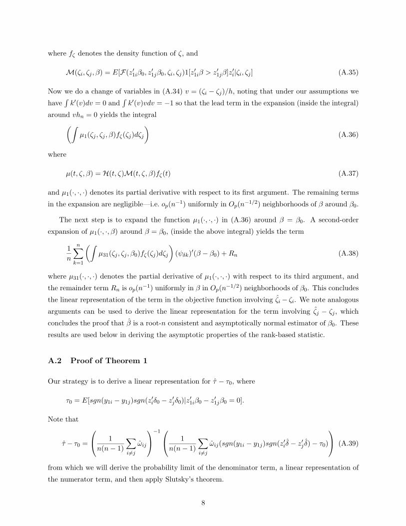
where fζ denotes the density function of ζ, and

M(ζi, ζj , β) = E[F(z′1iβ0, z′1jβ0, ζi, ζj)1[z′1iβ > z′1jβ]z′i|ζi, ζj ] (A.35)

Now we do a change of variables in (A.34) v = (ζi − ζj)/h, noting that under our assumptions we

have∫k′(v)dv = 0 and

∫k′(v)vdv = −1 so that the lead term in the expansion (inside the integral)

around vhn = 0 yields the integral(∫µ1(ζj , ζj , β)fζ(ζj)dζj

)(A.36)

where

µ(t, ζ, β) = H(t, ζ)M(t, ζ, β)fζ(t) (A.37)

and µ1(·, ·, ·) denotes its partial derivative with respect to its first argument. The remaining terms

in the expansion are negligible—i.e. op(n−1) uniformly in Op(n−1/2) neighborhoods of β around β0.

The next step is to expand the function µ1(·, ·, ·) in (A.36) around β = β0. A second-order

expansion of µ1(·, ·, β) around β = β0, (inside the above integral) yields the term

1n

n∑k=1

(∫µ31(ζj , ζj , β0)fζ(ζj)dζj

)(ψδk)′(β − β0) +Rn (A.38)

where µ31(·, ·, ·) denotes the partial derivative of µ1(·, ·, ·) with respect to its third argument, and

the remainder term Rn is op(n−1) uniformly in β in Op(n−1/2) neighborhoods of β0. This concludes

the linear representation of the term in the objective function involving ζi− ζi. We note analogous

arguments can be used to derive the linear representation for the term involving ζj − ζj , which

concludes the proof that β is a root-n consistent and asymptotically normal estimator of β0. These

results are used below in deriving the asymptotic properties of the rank-based statistic.

A.2 Proof of Theorem 1

Our strategy is to derive a linear representation for τ − τ0, where

τ0 = E[sgn(y1i − y1j)sgn(z′iδ0 − z′jδ0)|z′1iβ0 − z′1jβ0 = 0].

Note that

τ − τ0 =

1n(n− 1)

∑i 6=j

ωij

−1 1n(n− 1)

∑i 6=j

ωij(sgn(y1i − y1j)sgn(z′iδ − z′j δ)− τ0)

(A.39)

from which we will derive the probability limit of the denominator term, a linear representation of

the numerator term, and then apply Slutsky’s theorem.

8

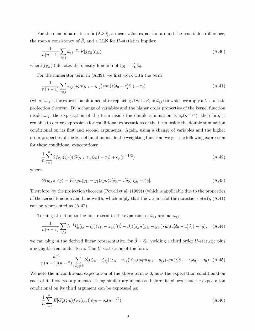
For the denominator term in (A.39), a mean-value expansion around the true index difference,

the root-n consistency of β, and a LLN for U -statistics implies:

1n(n− 1)

∑i 6=j

ωijp→ E[fZβ(ζβi)] (A.40)

where fZβ(·) denotes the density function of ζβi = z′1iβ0.

For the numerator term in (A.39), we first work with the term

1n(n− 1)

∑i 6=j

ωij(sgn(y1i − y1j)sgn(z′iδ0 − z′jδ0)− τ0) (A.41)

(where ωij is the expression obtained after replacing β with β0 in ωij) to which we apply a U -statistic

projection theorem. By a change of variables and the higher order properties of the kernel function

inside ωij , the expectation of the term inside the double summation is op(n−1/2); therefore, it

remains to derive expressions for conditional expectations of the term inside the double summation

conditional on its first and second arguments. Again, using a change of variables and the higher

order properties of the kernel function inside the weighting function, we get the following expression

for these conditional expectations:

1n

n∑i=1

2fZβ(ζβi)(G(y1i, zi, ζβi)− τ0) + op(n−1/2) (A.42)

where

G(y1, z, ζβ) = E[sgn(y1i − y1)sgn(z′iδ0 − z′δ0)|ζβi = ζβ]. (A.43)

Therefore, by the projection theorem (Powell et al. (1989)) (which is applicable due to the properties

of the kernel function and bandwidth, which imply that the variance of the statistic is o(n)), (A.41)

can be represented as (A.42).

Turning attention to the linear term in the expansion of ωij around ωij

1n(n− 1)

∑i 6=j

h−1k′h(ζi − ζj)(z1i − z1j)′(β − β0)(sgn(y1i − y1j)sgn(z′iδ0 − z′jδ0)− τ0), (A.44)

we can plug in the derived linear representation for β − β0, yielding a third order U -statistic plus

a negligible remainder term. The U -statistic is of the form:

h−1n

n(n− 1)(n− 2)

∑i 6=j 6=k

k′h(ζβi − ζβj)(z1i − z1j)′ψβi(sgn(y1i − y1j)sgn(z′iδ0 − z′jδ0)− τ0). (A.45)

We note the unconditional expectation of the above term is 0, as is the expectation conditional on

each of its first two arguments. Using similar arguments as before, it follows that the expectation

conditional on its third argument can be expressed as:

1n

n∑i=1

E[G′x(ζβi)fZβ(ζβi)]ψβi + op(n−1/2) (A.46)

9

where

Gx(·) = E[(sgn(y1i − y1j)sgn(z′iδ0 − z′jδ0)− τ0)(z1i − z1j)′|z1i − z1j = ·]

and G′x(·) denotes the derivative of Gx(·) with respect to its argument.

A final term to deal with in the linear representation of the statistic is

1n(n− 1)

∑i 6=j

ωijsgn(y1i − y1j)(sgn((zi − zj)′δ)− sgn((zi − zj)′δ0)) (A.47)

Here we can effectively expand the above term with δ around δ0. To do so, since the sign function is

not differentiable, we take the expectation of sgn((zi− zj)′δ) for any δ. Recall, as a normalization,

we set the last component of δ = 1 and assume its associated regressor was continuously distributed.

Here we let FZk|Z−k(·) denote the cdf of zki− zkj conditional on (z′−ki, z

′−kj) (where zki denotes the

last component of zi and z′−ki denotes the other components of zi). Consequently, we have:

E[sgn((zi − zj)′δ)|z−ki, z−kj ] = FZk|Z−k(∆z′−kijδ

(−k))

where ∆z−kij denotes the difference in the corresponding components of zi and zj , and δ(−k) denotes

the subvector of δ corresponding to z−ki. We can expand this conditional expectation evaluated at

δ around the conditional expectation evaluated at δ0:

FZk|Z−k(∆z′−kij δ

(−k)) = FZk|Z−k(∆z′−kijδ

(−k)0 )+fZk|Z−k

(∆z′−kijδ(−k)0 )∆z′−kij(δ−δ0)+Op(‖δ−δ0‖2)

where fZk|Z−k(·) denotes the density function of zki− zkj conditional on z′−ki, z

′−kj . Note that since

the sgn function is Euclidean and δ−δ0 is Op(n−1/2) (by using, e.g., Theorem 1 in Sherman (1994)),

the remainder term that arises from replacing the difference in sgn functions with their expectations

in (A.47) is op(n−1/2).

Next, by applying the same arguments as before, involving plugging in a linear representation

(this time for (δ − δ0)), and decomposing the resulting third order U -statistic, we get a linear

representation for (A.47). Specifically, let

G11(·) = E[sgn(y1i − y1j)fZk|Z−k(∆z′−kijδ

(−k)0 )∆z′−kij |ζβi = ·, ζβj = ·].

Then, we may conclude that (A.47) has the following linear representation

1n

n∑i=1

E[G11(ζβi)fZβ(ζβi)]ψδi + op(n−1/2). (A.48)

Finally, we note that is easy to show that the remainder term, which involves the product of β−β0

and δ − δ0, is op(n−1/2).

10

Therefore, collecting all our results, we may conclude that

τ − τ0 = E[fZβ(ζβi)]−1 1n

n∑i=1

(2fZβ(ζβi)(G(y1i, zi, ζβi)− τ0) + E[G′x(ζβi)fZβ(ζβi)]ψβi

+ E[G11(ζβi)fZβ(ζβi)]ψδi

)+ op(n−1/2), (A.49)

which establishes the theorem.

B Monte Carlo simulations

In this section, we report results of Monte Carlo simulations that examine the performance of the

proposed statistic (τ) as well as other alternative approaches for testing for presence of causal effects

(most notably the two-stage least-squares estimator (2SLS)). First, we consider a design (Design 1

below) in which both τ and 2SLS (as well as a correctly specified MLE estimator) are theoretically

justified testing approaches. This design has a binary outcome and a binary endogenous regressor

(with continuous instrument) but no additional covariates in the outcome equation; for this de-

sign, the results of Shaikh and Vylacil (2005) and Bhattacharya, Shaikh, and Vytlacil (2005) imply

that the probability limit of 2SLS identifies the correct sign of the treatment effect. The goal of

these simulations is to compare size and power of the alternative approaches to make sure that the

flexibility of the semiparametric (τ) approach does not adversely affect practical performance in a

simple setting. Second, we provide a simple design (Design 2 below) that serves as a cautionary

tale for using 2SLS (or ordinary least squares (OLS)) in order to test for causal effects in non-linear

models. Specifically, we consider a probit model (binary outcome) with no treatment effect and

no endogeneity. In general, when one moves beyond the binary-outcome/binary-treatment model

with no additional covariates, the non-linearity of the outcome equation will generally lead the

OLS or 2SLS estimators for the endogenous coefficient to have non-zero probability limits even

when the true coefficient is zero. The implication is that, under the null of no treatment effect,

rejection rates can approach 100% as the sample size grows. Finally, to demonstrate the robustness

of the semiparametric approach, we consider two designs (Designs 4 and 5 below) having additional

non-linearity and interactions in the covariate specification; for these designs, as in Design 3, we

compare the performance of the rank-based test statistic to both OLS and 2SLS.

Design 1: binary outcome, binary treatment, no additional covariates

The following simple design, with a continuous instrumental variable for the binary endogenous

regressor, is considered:

y1i = 1[α0y2i + εi > 0] (A.50)

11

y2i = 1[zi + ηi > 0] (A.51)

where zi is a standardized χ23 random variable (normalized to have mean zero and standard devi-

ation one) and

(εi

ηi

)∼ N

((0

0

),

(1 ρ0

ρ0 1

)). Two parameters, α0 (the coefficient on the

binary endogenous variable) and ρ0 (the correlation between ηi and εi), are chosen to vary over the

simulation designs. In particular, the values ρ0 = 0, 0.25, 0.50, 0.75 and α0 = 0, 0.1, 0.2, 0.3 are con-

sidered, yielding 16 different designs. For each of the 16 designs, 1,000 simulations were conducted

with a sample size of n = 500. Three different approaches to testing the significance of α (i.e.,

testing H0 : α0 = 0) were considered: (i) a full MLE estimation strategy (with the test based upon

the z-statistic of αmle), (ii) a linear IV estimation strategy (with the test based upon the z-statistic

of αiv, and (iii) the third-stage statistic τ proposed above (which, in this case, is the Kendall’s tau

correlation between y1i and zi). Table S1 summarizes the results, with rejection rates reported for

the 5% and 10% levels for the three approaches (labeled MLE, IV, and τ , respectively). The first

four rows of the table correspond to α0 = 0 and, therefore, provide evidence on the size of the test.

The rejection rates for the three tests are in line with the 5% and 10% levels, although at the higher

levels of correlation (ρ0 = 0.50 and ρ0 = 0.75) between the error disturbances, the MLE approach

exhibits some over-rejection. The remaining rows of the table provide evidence on the power of the

test (for α0 = 0.1, 0.2, 0.3). Overall, the power of the alternative approaches is remarkably similar

across these designs. For ρ0 = 0.75, the MLE approach does have higher rejection rates, but these

are likely the result of the over-rejection phenomenon seen in the α0 = 0/ρ0 = 0.75 design; for the

other ρ0 values, the MLE approach has rejection rates which are basically indistinguishable from

the other two approaches. For this simple Monte Carlo design, the semiparametric approach to

testing for significance of the binary endogenous variable compares favorably with both an MLE

approach and a linear IV approach.

Design 2: probit model with no treatment effect and no endogeneity

We consider a probit model having no treatment effect (a coefficient of zero on the y2 variable)

and no endogeneity. The y1 outcome equation has a covariate w, and y2 is related to an additional

“instrument” z:

y1i = 1[−3 + wi + ηi > 0] (A.52)

y2i = 1[−5 + wi + zi + εi > 0] (A.53)

with wi ∼ χ23, zi ∼ U [0, 4], εi ∼ N(0, 1), and ηi ∼ N(0, 1) independent of each other. For the Monte

Carlo simulations, we compared the performance of three approaches (OLS, 2SLS, and the τ -based

test) for testing significance of the causal effect of y2 upon y1. For OLS, we ran a regression of y1

on w and y2 (and an intercept) and computed the heteroskedasticity-robust z-statistic on the y2

12

coefficient. For 2SLS, the first-stage regression was OLS of y2 on w and z, and the second-stage

regression was OLS of y1 on w and the fitted y2 values from the first stage; we then computed the

heteroskedasticity-robust z-statistic on the y2 coefficient. For the τ statistic, we used the bootstrap

(50 replications) in order to compute standard errors and, in turn, z-statistics; the normal-density

kernel was used, and results for a bandwidth of h = 0.1 are reported (though results were similar

across a range of different bandwidths). Table S2 reports the results from 1,000 simulations for

sample sizes n ∈ 50, 100, 200, 400, 1000. Rejection rates for the 5%-level and 10%-level tests are

reported for the three different methods. Both the OLS and 2SLS methods are clearly incorrectly

sized. The OLS rejection rates for n = 50 are 16.0% and 25.5% and quickly diverge at higher

sample sizes (nearly 100% rejection rates at n = 1000). The 2SLS performs even worse for the

smallest sample size (28.9% and 38.5% rejection rates for n = 50), and the rejection rates remain

fairly stable (and incorrect) across the sample sizes considered. In contrast, the rank-based test

statistic appears to be properly sized. There is some evidence of over-rejection at n = 50 (9.1%

and 15.2$ rejection rates) but, at higher samples, the rejection rates are very close to the correct size.

Design 3: non-linear relationship between the instrument and endogenous variable

We consider a design similar to Design 1, except that the endogenous variable is continuous and is

a non-linear function of the instrumental variable. As in Design 1, we consider the simplest case

where there are no additional covariates. The goal is to examine what happens in a case where

we use 2SLS assuming that the instrument is zi but the reduced-form model for the endogenous

variable is instead a non-linear function of zi (specifically a square-root form in this design):

y1i = 1[5α0y2i + εi > 0] (A.54)

y2i = −1 +√zi/5 + ηi (A.55)

with√

6zi ∼ χ23 and (εi, ηi) has a bivariate normal distribution with zero means, unit vari-

ances, and correlation parameter ρ0. Like Design 1, we consider a set of 16 designs (with ρ0 ∈0.00, 0.25, 0.50, 0.75 and α0 ∈ 0.0, 0.1, 0.2, 0.3). To give a sense of how the non-zero α0 spec-

ifications differ from the α0 = 0 (no treatment) specification, we computed the average marginal

effects for these values — approximately 0.17, 0.26, and 0.30 for α = 0.1, α = 0.2, and α = 0.3,

respectively.

Using 1,000 simulations for n = 200, Table S3 reports rejection rates for OLS, 2SLS, and the τ -

based test at the 5% level. The OLS method clearly performs very badly, with the rejection rate at

α0 = ρ0 = 0 being fine (5.6%) but increasing to 81.6% for α0 = 0/ρ0 = 0.25 and 100% for all other

specifications. While the 2SLS appears to have greater power than the τ method, there is evidence

that the 2SLS method is incorrectly sized. In particular, there is significant under-rejection for the

α0 = 0 case when ρ0 ∈ 0, 0.25, 0.5.

13

Design 4: non-linearity and interaction in the outcome equation

The following design again exhibits non-linearity. In addition, however, we allow for an interaction

between the endogenous variable y2 and the exogenous-covariate index (in this case, just a single

exogenous variable w). Specifically, y1 has the following exponential specification:

y1i = exp(−wi − α0wiy2i + εi) (A.56)

y2i = −1 + zi + ηi (A.57)

with wi ∼ Bernoulli(0.5),√

6zi ∼ χ23, and (εi, ηi) has a bivariate normal distribution with zero.

This outcome equation falls within the generalized regression model since the endogenous variable

is interacting with the full covariate index (which in this simple case is just the wi variable itself).

Note that wi is a binary covariate here, with y1i = exp(εi) when wi = 0 and y1i = exp(−1−α0y2i+εi)

when wi = 1. For this design, we consider what happens when we use 2SLS of y1 on w and y2,

with z instrumenting for y2. Thus, the underlying model for this 2SLS regression is misspecified

in two ways: (i) the non-linearity is ignored (using y1 rather than ln(y1)) and (ii) the interaction

is ignored. For the OLS results, we regress y1 on w and y2. Again, we consider a set of 16 designs

(with ρ0 ∈ 0.00, 0.25, 0.50, 0.75 and α0 ∈ 0.0, 0.1, 0.2, 0.3). The last three columns of Table S3

report rejection rates for OLS, 2SLS, and τ at the 5% level, based upon 1,000 simulations for

n = 200. In contrast to Design 3, the 2SLS test appears to be appropriately sized in this design

(even in the presence of the non-linearity). For the α0 = 0.1 alternatives (the alternatives closest

to the null), the 2SLS and τ tests have comparable power. For the other alternatives (α0 = 0.2

and α0 = 0.3), however, the power of the τ test becomes much stronger than that of the 2SLS

test. Finally, as in the previous designs, we find that OLS vastly over-rejects in the presence of

endogeneity when there is no treatment effect present (50.5% rejection for α0 = 0/ρ0 = 0.25 and

increasing at higher ρ0 values).

C Empirical application

In this section, we apply our estimation and testing methodology to an empirical application con-

cerning the effects of fertility on female labor supply. In particular, we adopt the approach of

Angrist and Evans (1998), who use the gender mix of a woman’s first two children to instrument

for the decision to have a third child. This instrumental-variable strategy allows one to identify

the effect of having a third child upon the woman’s labor-supply decision. The rationale for this

strategy is that child gender is arguably randomly assigned and that, in the United States, families

whose first two children are the same gender are significantly more likely to have a third child.

Using 1980 and 1990 Census data, Angrist and Evans (1998) find that married women whose

first two children are the same gender are 5–8% more likely to have a third child; using the same-sex

14

indicator as an instrument for having a third child, they find that having a third child lowers the

probability of a married women working for pay by about 10–12%. Rather than using the 1980 and

1990 Census data, the sample for the current study is drawn from the 2000 Census data (5-percent

public-use microdata sample (PUMS)) in order to see if any interesting changes have occurred in

the relationship between fertility and labor supply. Starting from the household PUMS data, a

mother was retained in the sample if all of the following criteria were satisfied: (i) mother has two

or more children, (ii) mother is white, (iii) mother is a United States citizen, (iv) mother is married

with spouse present in household, and (v) oldest child is 12 years of age or younger.2 In addition,

to eliminate any families that might have twin births (or higher-order multiple births), any family

with same-aged first and second children or same-aged second and third children were dropped

from the sample. The resulting sample consists of 293,771 observations.

Summary statistics for the variables to be used in the analysis are provided in Table S4. The

table shows that 69.7% of mothers in the sample worked for pay during 1999 and 25.7% of mothers

had a third child. The percentage of women working for pay represents a very slight increase over

the comparable percentage from the 1990 Census data, and the percentage having a third child

represents a decline from 1990. In the analysis, the outcome of interest (y1) is whether the mother

worked in 1999, the binary endogenous explanatory variable (y2) is the presence of a third child,

and the instrument is whether the mother’s first two children were of the same gender.

Table S5 reports the first-stage regression results, i.e. regressing the have-third-child indicator

upon the same-sex indicator variable and the other z variables. The linear probability estimates

and the probit estimates indicate that mothers whose first two children are the same gender are

5.6–5.8 percentage points more likely to have a third child than mothers whose first two children

are of different gender. These estimates are very similar, although slightly lower in magnitude, to

those found by Angrist and Evans (1998, Table 5) for the earlier 1980 and 1990 samples. Table S6

reports the second-stage estimates for the (linear) two-stage least squares estimator, along with the

OLS estimates for comparison. Again, the results are very similar to those found by Angrist and

Evans (1998, Tables 7 and 8), with the OLS estimates of the had-third-child effect on labor supply

larger in magnitude than the 2SLS estimates.

Table S7 considers the alternative tests for significance of the binary endogenous regressor,

comparing the semiparametric τ test proposed in this paper with the z-test based upon the 2SLS

estimates. In order to examine the effect of additional covariates, testing results are reported

starting from a model with no exogenous covariates and then adding covariates onb-by-one until2The PUMS data contains information on children under the age of 18 that are living in the household. Unlike

earlier editions of the PUMS data, the 2000 edition does not contain a data item for the “total number of children

ever born.” Therefore, the last criterion is used in order to make it more likely that the oldest child in the household

is actually the mother’s first child. The cutoff could be lowered further to increase this certainty but at the expense

of decreasing the sample size.

15

the full set of three exogenous covariates are included. (Note that the 2SLS estimates and standard

errors for the no-covariate and three-covariate models correspond to those presented in Table S6.) In

the model with no exogenous covariates, the z-statistics associated with τ and the 2SLS coefficient

are extremely similar. This finding is very much in line with the Monte Carlo simulation evidence

(Design 1) of the previous section. The 2SLS z-statistic for the larger models is basically unchanged

from the no-covariate model, which is not too surprising given that the same-sex instrument is

uncorrelated with the other exogenous covariates in the model. In contrast, the magnitude of the

z-statistic for the semiparametric τ method does decline. The addition of covariates to the model

forces the semiparametric method to make comparisons based upon observation-pairs with similar

first-stage (estimated) index values associated with these exogenous covariates. It is encouraging,

however, that the z-statistic magnitude does not decline by much as the second and third covariates

are added to the model. Table S7 highlights the inherent robustness-power tradeoff between the

semiparametric and parametric methodologies. Although one might have worried that the tradeoff

would be so drastic to render the semiparametric method useless in practice, the results indicate

that this is not the case. Even in the model with three covariates, the τ estimate provides strong

statistical evidence (z = −2.69) that the endogenous third-child indicator variable has a causal effect

upon mothers’ labor supply. Importantly, this finding is not subject to the inherent misspecification

of the linear probability model or any type of parametric assumption on the error disturbances.

16

Table S1: Monte Carlo simulation results for Design 1 (binary outcome, binary treatment, no

additional covariates) with n = 500. Rejection rates (over 1,000 simulations) for tests at the

5% and 10% levels are reported. The three different z-tests are based upon MLE estimation, IV

estimation, and rank correlation.

5%-level rejections 10%-level rejections

ρ0 α0 MLE IV τ MLE IV τ

Size of the test 0.00 0.0 0.054 0.051 0.040 0.091 0.099 0.087

0.25 0.0 0.062 0.050 0.056 0.109 0.094 0.109

0.50 0.0 0.065 0.054 0.047 0.120 0.107 0.085

0.75 0.0 0.069 0.048 0.057 0.131 0.102 0.105

Power of the test 0.00 0.1 0.071 0.075 0.071 0.134 0.144 0.126

0.25 0.1 0.099 0.106 0.091 0.153 0.163 0.160

0.50 0.1 0.087 0.092 0.083 0.155 0.157 0.144

0.75 0.1 0.099 0.090 0.086 0.160 0.153 0.152

0.00 0.2 0.161 0.168 0.162 0.265 0.269 0.251

0.25 0.2 0.174 0.180 0.176 0.272 0.271 0.280

0.50 0.2 0.180 0.176 0.167 0.279 0.256 0.261

0.75 0.2 0.241 0.222 0.225 0.361 0.328 0.332

0.00 0.3 0.310 0.303 0.298 0.419 0.399 0.414

0.25 0.3 0.315 0.302 0.324 0.440 0.428 0.437

0.50 0.3 0.321 0.338 0.327 0.447 0.442 0.430

0.75 0.3 0.439 0.420 0.418 0.587 0.543 0.528

Table S2: Monte Carlo simulation results for Design 2 (probit model with no treatment effect and

no endogeneity). Rejection rates (over 1,000 simulations) for z-tests at the 5% and 10% levels are

reported.

OLS 2SLS τ

n 5% level 10% level 5% level 10% level 5% level 10% level

50 0.169 0.255 0.289 0.385 0.091 0.152

100 0.309 0.427 0.273 0.356 0.055 0.104

200 0.524 0.648 0.290 0.386 0.045 0.091

400 0.831 0.901 0.256 0.350 0.055 0.106

1000 0.993 0.998 0.237 0.337 0.056 0.101

17

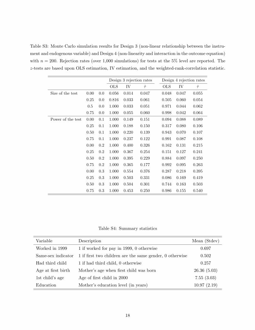
Table S3: Monte Carlo simulation results for Design 3 (non-linear relationship between the instru-

ment and endogenous variable) and Design 4 (non-linearity and interaction in the outcome equation)

with n = 200. Rejection rates (over 1,000 simulations) for tests at the 5% level are reported. The

z-tests are based upon OLS estimation, IV estimation, and the weighted-rank-correlation statistic.

Design 3 rejection rates Design 4 rejection rates

OLS IV τ OLS IV τ

Size of the test 0.00 0.0 0.056 0.014 0.047 0.048 0.047 0.055

0.25 0.0 0.816 0.033 0.061 0.505 0.060 0.054

0.5 0.0 1.000 0.033 0.051 0.971 0.044 0.062

0.75 0.0 1.000 0.055 0.060 0.998 0.042 0.064

Power of the test 0.00 0.1 1.000 0.149 0.151 0.094 0.088 0.089

0.25 0.1 1.000 0.188 0.150 0.317 0.080 0.106

0.50 0.1 1.000 0.220 0.139 0.943 0.070 0.107

0.75 0.1 1.000 0.237 0.122 0.991 0.087 0.108

0.00 0.2 1.000 0.400 0.326 0.162 0.131 0.215

0.25 0.2 1.000 0.367 0.254 0.151 0.127 0.241

0.50 0.2 1.000 0.395 0.229 0.884 0.097 0.250

0.75 0.2 1.000 0.365 0.177 0.992 0.095 0.263

0.00 0.3 1.000 0.554 0.376 0.287 0.218 0.395

0.25 0.3 1.000 0.503 0.331 0.086 0.169 0.419

0.50 0.3 1.000 0.504 0.301 0.744 0.163 0.503

0.75 0.3 1.000 0.453 0.250 0.986 0.155 0.540

Table S4: Summary statistics

Variable Description Mean (Stdev)

Worked in 1999 1 if worked for pay in 1999, 0 otherwise 0.697

Same-sex indicator 1 if first two children are the same gender, 0 otherwise 0.502

Had third child 1 if had third child, 0 otherwise 0.257

Age at first birth Mother’s age when first child was born 26.36 (5.03)

1st child’s age Age of first child in 2000 7.55 (3.03)

Education Mother’s education level (in years) 10.97 (2.19)

18

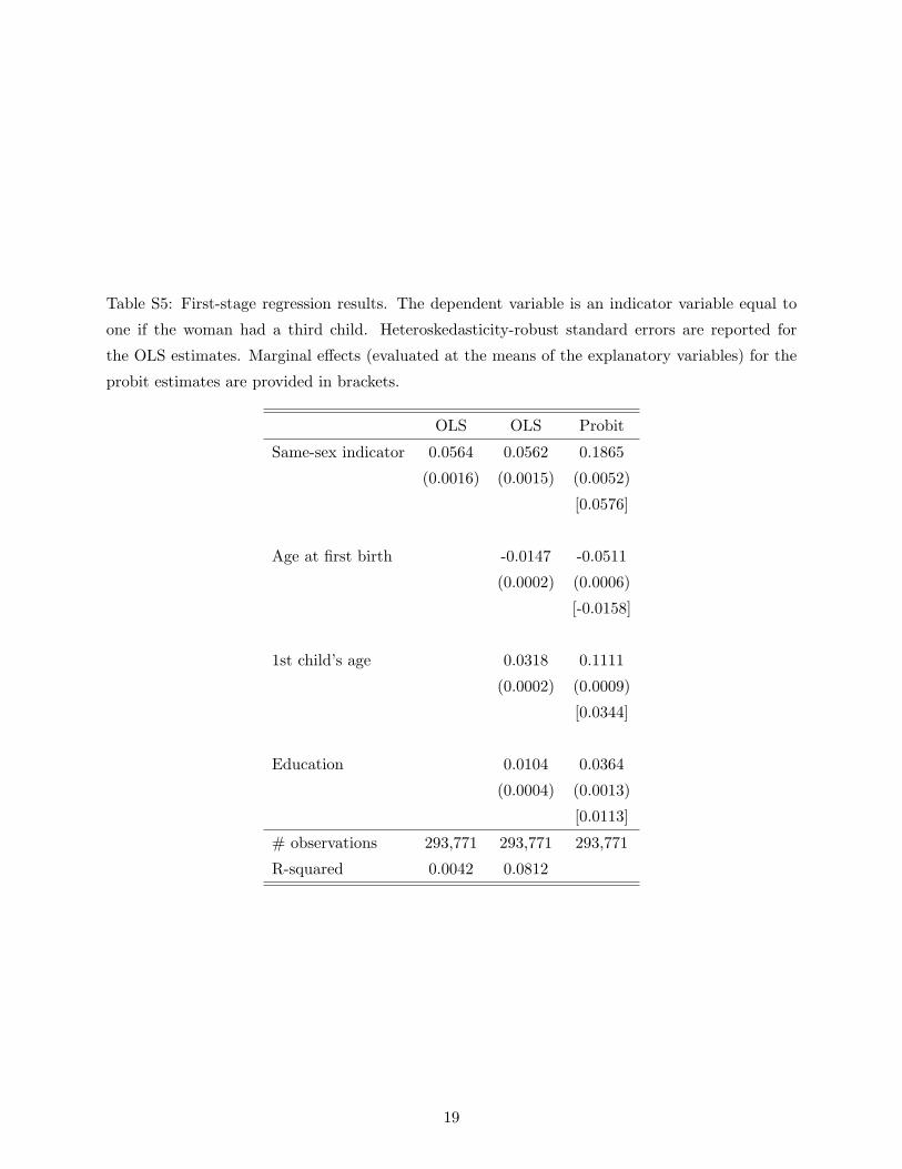
Table S5: First-stage regression results. The dependent variable is an indicator variable equal to

one if the woman had a third child. Heteroskedasticity-robust standard errors are reported for

the OLS estimates. Marginal effects (evaluated at the means of the explanatory variables) for the

probit estimates are provided in brackets.

OLS OLS Probit

Same-sex indicator 0.0564 0.0562 0.1865

(0.0016) (0.0015) (0.0052)

[0.0576]

Age at first birth -0.0147 -0.0511

(0.0002) (0.0006)

[-0.0158]

1st child’s age 0.0318 0.1111

(0.0002) (0.0009)

[0.0344]

Education 0.0104 0.0364

(0.0004) (0.0013)

[0.0113]

# observations 293,771 293,771 293,771

R-squared 0.0042 0.0812

19

Table S6: Second-stage regression results. The dependent variable is an indicator variable equal to

one if the woman worked for pay in 1999. The 2SLS regressions use the same-sex indicator variable

as an instrument for the had-third-child indicator variable. Heteroskedasticity-robust standard

errors are reported.

OLS 2SLS OLS 2SLS

(Wald)

Had third child -0.1382 -0.1118 -0.1728 -0.1124

(0.0020) (0.0298) (0.0020) (0.0295)

Age at first birth -0.0074 -0.0065

(0.0002) (0.0005)

1st child’s age 0.0161 0.0142

(0.0003) (0.0010)

Education 0.0319 0.0313

(0.0004) (0.0005)

# observations 293,771 293,771 293,771 293,771

R-squared 0.0173 0.0167 0.0462 0.0432

20

Table S7: Testing significance of the binary endogenous regressor. The z-statistics for the semi-

parametric and 2SLS estimation approaches are reported for several different model specifications.

The 2SLS standard errors are heteroskedasticity-robust.

Exogenous covariates Semiparametric 2SLS

in the model τ s.e. z-stat α s.e. z-stat

None -0.00316 0.00085 -3.72 -0.1118 0.0298 -3.75

Education -0.00299 0.00102 -2.94 -0.1103 0.0296 -3.72

Education, -0.00655 0.00229 -2.86 -0.1111 0.0296 -3.75

Mother’s age at first birth

Education, -0.00695 0.00258 -2.69 -0.1124 0.0295 -3.80

Mother’s age at first birth,

Age of 1st child

21