A Quarterly Transactions-Based Index (TBI) of Institutional Real Estate Investment Performance and Movements in Supply and Demand

by

Jeff Fisher*, David Geltner**, & Henry Pollakowski*** MIT Center for Real Estate

May 2006 (Note: This is the manuscript of: J Real Estate Finan Econ (2007) 34:5–33 © Springer)

Abstract

This article presents a methodology for producing a quarterly transactions-based index (TBI) of property-level investment performance for U.S. institutional real estate. Indices are presented for investment periodic total returns and capital appreciation (or price-changes) for the major property types included in the NCREIF Property Index. These indices are based on transaction prices to avoid appraisal-based sources of index “smoothing” and lagging bias. In addition to producing variable-liquidity indices, this approach employs the Fisher-Gatzlaff-Geltner-Haurin (REE 2003) methodology to produce separate indices tracking movements on the demand and supply sides of the investment market, including a “constant-liquidity” (demand side) index. Extensions of Bayesian noise filtering techniques developed by Gatzlaff & Geltner (REF 1998) and Geltner & Goetzmann (JREFE 2000) are employed to allow development of quarterly frequency, market segment specific indices. The hedonic price model used in the indices is based on an extension of the Clapp & Giacotto (JASA 1992) “assessed value method”, using a NCREIF-reported recent appraised value of each transacting property as the composite “hedonic” variable, thus allowing time-dummy coefficients to represent the difference each period between the (lagged) appraisals and the transaction prices. The index could also be used to produce a mass appraisal of the NCREIF property database each quarter, a byproduct of which would be the ability to provide transactions price based “automated valuation model” estimates of property value for each NCREIF property each quarter. Detailed results are available at http://web.mit.edu/cre/research/credl/tbi.html.

Methodology update, May 2009: The following changes in methodology and production procedures will be made for the TBI as of 1Q09:

• Published indexes will be frozen as of the end of each calendar year. This is for the convenience of users, and reflects experience indicating that backward-adjustments have been minimal and not of economic significance.

• Published indexes will be based on a starting value of 100 as of the inception date of each index (1984Q1 for all-property, 1994Q1 for the sectoral indexes).

• The ridge regression noise filter will be eliminated going forward starting 1Q09 for the all-property index only. Experience indicates that in the all-property index the noise filter has little impact and is not needed subsequent to the early history of the index (where effectively the filter is retained by the freezing of the prior history). Eliminating the noise filter will enable the all-property index to be more independent of the NPI during the preliminary quarterly reports.

• Going forward starting in 1Q09 the “representative property” used to compute the index based on the hedonic price model will have its “hedonic value” (based on the self-reported NPI valuations) re-set to be lagged 2 quarters prior to the current NPI

1

appreciation level. Experience indicates that NCREIF self-reported valuations are now less lagged than they used to be, suggesting that this change is warranted based on the specification of the quarterly hedonic price model.

• Each index will be published no matter how few are the current transactions observations unless in the judgment of the MIT/CRE TBI manager (presently David Geltner) there is both extremely few current observations and a spurious or implausible-seeming estimated return. If an index must be skipped due to lack of observations the circumstances will be described in the published quarterly commentary and the index will be back-filled by “straight-lining” as soon as data is next available. (This is the procedure followed for the retail index for 4Q2008-1Q2009.)

2

A Quarterly Transactions-Based Index (TBI) of Institutional Real Estate Investment Performance and Movements in Supply and Demand

by

Jeff Fisher*, David Geltner**, & Henry Pollakowski***

MIT Center for Real Estate

“In summary, we argue that the NCREIF Index is ready to evolve into two more specialized successor families of index products: one tailored for fundamental asset class research support, and the other tailored for investment performance evaluation benchmarking and performance attribution.” -- From: D.Geltner & D.Ling, Benchmarks & Index Needs in the U.S. Private Real Estate Investment Industry: Trying to Close the Gap (A RERI Study for the Pension Real Estate Association), October 17, 2000.

This article addresses the need for a “fundamental asset class research” index of

real estate investment performance and market conditions by presenting a state-of-the-art

transactions-based index (TBI) of commercial real estate. The TBI does not replace the

appraisal-based NCREIF Property Index (NPI), but complements it.1 It applies modern

econometrics to distill information from property transaction prices and results in an index

that provides the academic and industry investment research communities with certain

useful characteristics that the appraisal-based NPI lacks.2

Since the advent of modern portfolio theory and rigorous investment management

and analysis almost 50 years ago, asset classes in the core of the institutional investment

portfolio have required indices of total returns that accurately track investment performance

1 See Geltner & Ling (2001, 2005). 2 As of 2006, this index is being produced by the Commercial Real Estate Data Laboratory at the MIT Center for Real Estate. The TBI is updated quarterly within 45 days of the end of each quarter, and is available to the public. See http://web.mit.edu/cre/research/credl/tbi.html.

3

and which reflect the state of the market for the asset class. The NPI was developed over a

quarter century ago to address this need for real estate.

While the NPI is quite useful, and appropriate for many functions (e.g., as a

benchmark for investment manager performance), the research community has never been

entirely satisfied with it . The NPI is based on appraised values of the properties in the

index. Given the nature of the appraisal process, and because most properties in the index

are not fully or independently reappraised every quarter, the index exhibits a degree of

“smoothing” and “lagging” relative to the underlying real estate market.3 This can be

problematic for some research and analysis purposes, such as some types of multi-asset

class studies and comparisons (including portfolio optimization), and studies of market

turning points or historical market conditions. Although techniques have been developed to

“unsmooth” or “reverse-engineer” the NPI to eliminate the smoothing and lagging, these

techniques are inevitably somewhat ad hoc or mathematically complex, and difficult for the

broader investment community to understand.4

Thus studies of the fundamental nature and characteristics of the real estate asset

market would greatly benefit from an accurate and transparent transactions-based index

that avoids the smoothing and lagging in the NPI. As the NCREIF Index has matured, its

database has grown to include a sufficiently large number of property transactions,

meaning that in combination with recent developments in econometric methodology, it is

3 See for example: Geltner & Miller (2001), Chapter 25; and for a literature review: Geltner, MacGregor & Schwann (2003). 4 See for example: Brown (1985), Blundell & Ward (1987), Quan & Quigley (1989, 1991); Geltner (1991); Giacotto & Clapp (1992); Geltner(1993); Fisher, Geltner & Webb (1994); Lai & Wang (1998); Fisher & Geltner (2000), Fu (2003).

4

possible to produce a useful transactions-based index from the NCREIF database. The

transaction-based index (TBI) is characterized by the following features:

• It is transactions-based index, calibrated directly on the transaction prices of

properties sold each quarter from the NPI database, although it also makes use of all

the information available in the appraisal-based officially-reported values of all of

the properties in the NPI.

• It is capable of on-going, regular production at the quarterly frequency, reporting

total investment return as well as the capital appreciation return component each

quarter, at the all-property level and at the level of the four major property sectors:

office, industrial, retail, and apartment.

• It could be used for the “mass appraisal” of all properties in the NPI database every

quarter, enabling an up-to-date, transactions price based estimate of the value of

each property (though such property-level valuation cannot be reported publicly as

it would violate NCREIF’s masking guidelines).

• It is based on state-of-the-art econometric techniques developed recently in the real

estate economics academic community, including correction for possible sample

selection bias in the sold properties and noise filtering at the quarterly frequency.

• In addition to a standard transactions price based index that reflects the pro-cyclical

variable liquidity in the real estate asset market, the TBI allows separate estimation

of movements on the demand side and on the supply side of the institutional

property market. The demand side index can be interpreted as a “constant liquidity

5

index” (CLI), which collapses both price and trading volume measures of changes

in market conditions into a single metric, the percentage change in price that would

allow a constant expected time on the market or constant turnover ratio of trading

volume in the market.

The TBI exhibits some of the major characteristics that we would expect from a

transactions-based index. It shows evidence of leading the NPI in time based on the timing

of the turning points of the major historical cycle in the asset market, and it exhibits greater

volatility and less autocorrelation (less inertia), including less seasonality. Furthermore, the

additional volatility seems to “make sense”, including quarterly down-ticks during notable

historical moments when we would expect the property market to have fallen at least

temporarily (but when the NPI does not register losses), such as the tax act of 1986

(unfavorable to real estate), the stock market crash of 1987, the Gulf War of 1991, the

financial crisis of 1998, the September 2001 terrorist attack, and the start of the Iraq War in

2003.

The remainder of this article is organized as follows. Section 1 presents the basic

theory and methodology on which the TBI is based, including its extension to include

demand and supply indices. Section 2 describes the data and the specific estimation and

index construction techniques used in the index. Section 3 presents the index development

results, and some basic analysis of the index returns, including a simple portfolio

optimization analysis. A conclusion section summarizes.

1. Theory and Methodology

6

To facilitate understanding not only of the variable liquidity transactions index but

also of the demand and supply indices, we must begin with a fundamental model of the

processes underlying the observed transaction prices and the observed volume of

transactions each period within the NCREIF population of properties. The model we use

was developed by Fisher, Gatzlaff, Geltner, and Haurin (2003), referred to hereafter as

FGGH. The indices presented in this paper are based on this model, with some

enhancements to the specific estimation methodology, which we will describe here.

The FGGH model represents a double-sided search market with heterogeneous

participants and heterogeneous properties. Observable transaction prices and observable

transaction volume both derive from interaction between two populations of market

participants: potential buyers (non-owners) on the demand side, and potential sellers

(owners) on the supply side. The model is depicted graphically in Exhibit 1, with the three

panels showing three successive points in time. The horizontal axis depicts reservation

prices, and the bell-shaped curves show the frequency distributions of potential buyers’ (the

left-hand curve) and potential sellers’ (the right-hand curve) reservation prices. The

dispersion depicted in these reservation price distributions reflects the heterogeneity of

individual market participants’ perceptions of values of the properties (as well as their

differing search costs, etc). The overlap between the distributions allows for profitable

trading of properties, as reflected in observed transaction volume. As time passes and news

arrives, both the buyer and seller populations revise their reservation prices, but not

necessarily in identical ways. The result is that the overlap region varies over time,

corresponding to variation in the trading volume (the turnover ratio or “liquidity”) within

the population of properties. Pro-cyclical variable liquidity, that is, greater transaction

7

volume during “up” markets (which is a striking empirical fact in real estate markets),

suggests that the demand side (potential buyers) reservation price distribution moves

quicker and/or farther than the supply side (potential sellers) reservation price distribution,

in response to the arrival of news relevant to value.

-------------------------------------

Insert Exhibit 1 about here.

-------------------------------------

Hedonic modeling controls for heterogeneity across properties, and Heckman’s

procedure controls for sample selection bias in the transacted properties by modeling both

transaction price and transaction sales propensity. By modeling both price and sale

probability it is possible to identify property value (i.e., reservation price) equations

separately for both the buyer population and the seller population. The buyers’ valuations

provide the demand side valuations and the constant-liquidity index, while the sellers’

valuations provide the supply side index. The specifics of the methodology are presented

below, which is an extension of FGGH.

On the demand side of the market is a population of potential buyers whose

reservation prices are modeled by equation (1):

(1) bittZb

tijtXbj

bitRP εβα ++= ∑∑

Similarly, on the supply side of the market is a population of potential sellers (owners)

whose reservation prices are modeled by equation (2)

8

(2) sittZs

tijtXsj

sitRP εβα ++= ∑∑

In these equations, the variables are described below:

bitRP , s

itRP = the natural logarithm of a buyer’s (seller’s) reservation price for

asset i as of time t (the price at which agents will stop searching or negotiating and agree to an immediate transaction);

bitε , = normally distributed mean zero random errors (reflecting heterogeneity

within the buyer and seller populations, respectively);

sitε

ijtX = a vector of j asset-specific characteristics of the properties relevant to

valuation (the “hedonic” variables);

tZ = a vector of zero/one time-dummy variables (Zt =1 in quarter t).

In (1) and (2), the ∑ and components reflect systematic asset-

specific values common to all potential buyers and all potential sellers, respectively.

Temporal variation is possible in the (hence the t in the subscript), reflecting variation

over time in the perceived hedonic quality of the property. In typical applications of real

estate hedonic value modeling the vector consists of a number of qualitative and

quantitative dimensions of property utility, such as size, age, location, etc. In the case of

commercial investment property valuation, many of these hedonic dimensions of utility

would be summarized quantitatively in the rent that the property can charge (which, of

course, also relates directly to the financial valuation of the asset).

ijtXbjα ∑ ijtXs

jα

ijtX

ijtX

9

Within the NCREIF database, an even more complete summary of the value of

the property is the most recent appraised value of the property. In the spirit of the Clapp

& Giacotto (1992) “assessed value method”, the most recent appraised value of each

property in the database may be used as a summary statistic collapsing the entire

vector into a single scalar value for each property in each time period. We will label this

variable

ijtX

itA and note that it clearly reflects both cross-sectional and temporal dispersion.

Thus, the and components are simplified to: and .∑ ijtXbjα ∑ ijtXs

jα itb Aα it

s Aα 5

The dispersion within the buyer reservation price distribution is governed by the

dispersion in , while the dispersion within the seller distribution is governed by .

These error terms are random, varying across the individual potential buyers and across

individual potential sellers, reflecting unobservable characteristics of the parties and their

perceptions of the properties.

b s

b s

b s

b

itε itε

In contrast, the btβ and coefficients represent systematic and common factors

across all buyers and all owners (respectively), within each period of time. and are

also common across all assets (i) within each period of time (like a time-varying

“intercept”), reflecting the population as a whole during period t. The combined effect of

the differences between the and coefficients (given the current values of A

stβ

tβ tβ

α α it), and

between the and coefficients is therefore what distinguishes the buyer and seller tβstβ

5 Note that since the reservation price model is in log values, we would also take the log of the appraised value.

10

reservation price distributions systematically from each other, each period. These

population-specific responses govern the central tendency within each population, in each

period of time.

Movements over time in the valuations’ central tendencies are reflected in the

changes over time in the or components, for the

buyers and sellers respectively. Such value changes over time may be due either to changes

over time in the values of the

⎟⎠⎞⎜

⎝⎛ ∑+ tZb

titAb βα ⎟⎠⎞⎜

⎝⎛ ∑+ tZs

titAs βα

itA summary hedonic variables (which reflect both cross-

sectional and longitudinal dispersion), or to the periodic variation in the and

parameters (which reflect purely longitudinal changes in the “intercepts”, or valuation

components not otherwise captured in the

b stβ tβ

itA variables). In the present NCREIF

application in which we are using each property’s recent appraisal (as of record 2 quarters

previously) as the catch-all hedonic variable, the intercepts will reflect primarily only

the difference each period between the central tendency of the appraisals and the central

tendency of the transaction prices, for period t.

tβ

Transactions are consummated when and only when the buyer’s reservation price

exceeds the seller's: RPbit ≥ RPs

it. Only under this condition do we observe a transaction

price, Pit. In other words, consistent with rational investment decision-making (NPV

maximization):

(3) ⎪⎩

⎪⎨⎧

<−

≥−=

. 0 if ,

0 if ,s

itRPbitRPunobserved

sitRPb

itRPobserveditP

11

The observed transaction price must lie in the range between the buyer’s and

seller’s reservation prices, both of which are unobserved. The exact price depends on the

outcome of a negotiation, and depends on the strategies and bargaining power of the two

parties. To produce demand and supply indices, we follow FGGH and assume that the

transaction price will equal the midpoint between the buyer’s and seller’s reservation

prices.6

Using (1) through (3) and our midpoint price assumption, we see that among sold

assets the expected transaction price (for asset i as of time t) is:

[ ] ( ) ( )[ ]sit

bit

sit

bitit

sj

bj RPRPEAE

t tZst

btitP ≥+∑+= +⎟

⎠⎞⎜

⎝⎛ ++ εεαα ββ

21

21

21 . (4)

The expectation of the sale price consists of three components: the expected midpoint

between the asset-specific buyer and seller perceptions of value, the midpoint between the

market-wide buyer and seller period-specific intercepts, and the expected value of the

random error, which is itself the midpoint between the buyer’s and seller’s random

components among the parties that consummate transactions. This last term is, in general,

nonzero, because of the condition that the buyer’s reservation price must exceed the seller’s

reservation price in any observable consummated transaction.

6 There is no reason to assume that either side of the negotiation will systematically have greater bargaining power or negotiating ability. Our assumption of trades at the midpoint is more realistic and more general than the assumption used in many previous studies in the real estate literature that all trades are at the buyer’s offer price, and the midpoint price assumption is consistent with Wheaton’s (1990) model of the housing market as a double-sided search market. However, within the framework developed in this section it is technically straightforward to replace the midpoint assumption with other specific assumptions (for example, allowing variable pricing across the cycle). Analysis available from the authors suggests that alternative assumptions yield results either similar to, or empirically less plausible than, the results obtained from the midpoint price assumption.

12

We can measure E[Pit] by estimating (4) via the following regression based on

observed transaction prices within the NCREIF population:

)( sit

bititit RPRPAaP itt tZt ≥∑= ++ εβ (5)

where: ⎟⎠⎞⎜

⎝⎛ += sba αα

21 , ( )s

tbtt βββ +=

21 , and ( )s

itbitit εεε +=

21 (and recall that Zt is a

zero/one time-dummy). Such a model will predict an estimated value, , for each property

i in each period t within the NCREIF population.

itP

As noted, the stochastic error term in (5) may have a nonzero mean because the

observed transaction sample consists only of selected assets, namely, those for which RPbit

RP≥ sit. If ([ ) ] 0≠≥+ itititit RPRPE εε sbsb , this will cause simple OLS estimation of (5) to

have biased coefficients. As described in FGGH, this sample selection bias problem can

be corrected by the well known Heckman procedure which involves estimation of a

separate probit model of property sale probability.

In our context, this sales model is useful not only in the Heckman procedure to

correct for sample selection bias in the value model, but also to enable separate

identification of the buyers (demand side) and sellers (supply side) valuation models, the

former of which presents the constant liquidity valuation, as described in FGGH.

13

The probit model of property sale probability is based fundamentally on the

decision of whether to sell an asset or not. The latent variable describing the decision for

the i-th asset in period t is : *itS

sitRPb

itRPitS −=* . (6)

*itS is not observable, only the outcome itS is observed:

(7) ⎪⎩

⎪⎨⎧ ≥=

otherwise. if ,00* ,1 itSif

itS

In other words, a sale occurs if and only if RPbit ≥ RPs

it, in which case Sit = 1, otherwise Sit

= 0.

Equation (6) defines *itS to equal the difference between the buyer’s and seller’s

reservation prices for the asset. Subtracting (2) from (1) as in (6) yields:

)()(* )( sit

bittZs

tbtitS it

sb A εεββαα −+−+= ∑− . (8)

Following FGGH, define: , , and . The Zsb ααω −= st

btt ββγ −= s

itbitit εεη −= t

variable here is the same as that in (1), (2), and (5), a zero/one time-dummy variable.

Equations (7) and (8) can be estimated as a probit model:

[ ] [ ]∑+Φ== ttitit ZAS γω1Pr (9)

14

where is the cumulative density function (cdf) of the normal probability distribution

evaluated at the value inside the brackets, based on and . The probit model estimates

the coefficients and residuals only up to a scale factor. The estimated coefficients in (9)

are and , and the estimated error is

[ ]Φ

itA tZ

σω / σγ /t ση /it , where . Label

the estimated probit coefficients

)( ititVar2 sb εεσ −=

tω ( ) σαασωω ˆˆ −==ˆ and tγ ˆˆˆ sb , and ˆ , so that:

( ) σββσγγ ˆˆˆ tttt −== ˆˆ sb .

This allows unbiased and consistent estimation of the price model, which is thus

modified from (5) to include the inverse Mills ratio, itλ , as indicated in equation (10)

below.7

. (10) itittZtitP itAa υλεησβ +++= ∑

As equation (10) is estimated based on a sample of transaction prices, this model

allows the construction of a transaction-based index of the NCREIF population of

properties. This can be done in at least two ways, both of which begin with the price

model’s predicted value of each property, each period:

ittZtitP itAa λεησβ ˆˆˆ ˆ ++= ∑ (11)

The TBI that we have constructed is based on a “representative property” p. Property p is

characterized by a typical or average value of itA and of itλ each period, and also by a

typical income flow (call it CFpt ). Then, the index returns are based on the predicted 7 As described in the FGGH (2003) appendix, σ is a standard output of econometric software packages that implement the Heckman procedure. Such packages also correct for heteroskedasticity in the procedure.

15

value of property p each period and property p’s cash flow each period. Thus, in perio

the capital return for Property p (and by construction, for the index as well) is:

d t

8

( ) ]ˆexp[]ˆexp[]ˆexp[ 11 −−−= ptptptpt PPPg (12a)

and the income return is:

( ) ]ˆexp[ 1−= ptptpt PCFy (12b)

and the total return is:

rpt = gpt + ypt (13)

A second way to construct an index is “mass appraisal”. In this approach equation

(11) is used to produce an estimated value of each property in the NPI database, each

period: itP . The total return and capital return is then computed for each property, each

period, in the same manner as above for the representative property:

ititit

itit

it

it

it

itititit gy

PPP

PCF

PPPCFr +=

−+=

−+=

−

−

−−

−

]ˆexp[]ˆexp[]ˆexp[

]ˆexp[]ˆexp[]ˆexp[]ˆexp[

1

1

11

1 (14)

Then these individual property returns are aggregated across all properties in the NPI

e-

:

each period. The aggregation may be by equal-weighting across the properties, or valu

weighting (as in the official NPI). In the case of the latter the index return is computed as

8 Recall that is in log levels. Exponentiation is required to convert from log levels to straight levels to define a simple periodic geometric return index instead of a continuously-compounded return index.

ptP

16

∑ ∑ ⎥⎥⎥

⎦

⎤

⎢⎢⎢

⎣

⎡

⎟⎟⎟

⎠

⎞

⎜⎜⎜

⎝

⎛=

−

−

iit

iit

itt r

PPr

]ˆexp[]ˆexp[

1

1 (15a)

In the former case (equal weighting), it is simply:

∑=

=tN

i t

itt N

rr1

(15b)

where Nt is the total number of properties in the NPI in period t.

Because the underlying hedonic value model (10) is a log value model, the above-

described mass appraisal procedure will result in a slight bias in the estimated straight

level values obtained from exponentiating the predicted log values of (11), and this bias

will induce a slight error (but no bias) in the return index.9 These effects are very minor

and may be corrected through well known mathematical adjustments (Neyman and Scott,

1960; Goldberger, 1968; Miller, 1983).

Note that the estimation of each individual property’s value as of each period via

equation (11) not only enables the construction of a mass appraisal index, but also allows

provision of the transactions-based estimated value of each property each period, a value

that might be of interest to the property owners.

The above described procedures, based on the price model in equation (10),

provide transactions-based versions of the NCREIF Index. As noted above, we use the

representative property approach in our TBI. As the hedonic variable is represented by 9 The mathematical rule known as "Jensen's Inequality", combined with the concavity of the log function, causes the average of the logs to always be less than the log of the average. This results in a slight downward bias in the estimated log value level in equation (11). itP

17

the current appraised value of each property each period, Ait , it is easy to see how this

model incorporates all of the information available in the appraisals, and adds to that any

additional information conveyed by the current transaction prices of properties sold from

the NPI during period t. The estimated value of each property is simply its appraised

value (lagged 2 quarters) plus the coefficient on the time dummy variable corresponding

to the current quarter t. The time-dummy coefficient reflects the difference between the

value indication implied by current transactions minus that implied by the appraisal. To

the extent that transaction prices are more current than these appraised values, the value

model will capture that difference.10

It is important to note that the result up to here provides what can accurately be

described as a variable liquidity index. That is, while the index accurately represents

typical transaction prices prevailing among consummated deals in the market each

quarter, such prices reflect varying ease or ability to sell properties across time. In other

words, the index reflects varying transaction volume or turnover, and hence, varying

“liquidity” over time (as thusly defined). This is because liquidity, as indicated by trading

volume or transaction frequency, varies over time in the commercial real estate

investment market. Furthermore, this variation is systematic and pro-cyclical, with

greater liquidity during “up” markets, and less during “down” markets.11 Elaborating

from FGGH, the above-described variable-liquidity valuation and returns estimates can

10 It should be noted that when estimated on a pooled database this model specification cannot avoid a potential danger of collinearity between the appraised value variable and some of the time-dummy variables. Such collinearity could cause an under-estimation of some of the time-dummy coefficients, which could cause the resulting index to understate the difference between the transaction price based valuations and the appraisal-based NPI valuations. This point will be discussed further later in this paper. 11 One cause of such variable liquidity in the NPI could be a type of “self-fulfilling prophecy” of transactions occurring at or near appraised values, first suggested by Fisher, Geltner, & Webb (1994). If NCREIF members are under pressure not to sell properties at prices below appraised value, and if appraised values lag behind market values, then it will be difficult to sell properties during down markets.

18

be adjusted to reflect constant liquidity over time (that is, constant “ease of selling”, or

constant expected time-on-the-market). As described below, this procedure also allows

the separate identification of indices of demand side and supply side valuations and

market movements over time. Indeed, the index of movements on the demand side of the

market is the “constant liquidity” index.12

We begin by recalling that equation (10) provides a model of observed

equilibrium transaction prices in the relevant property market while equation (9) provides

a model of observed equilibrium transaction volume in that market as reflected in the sale

probability of a given asset. Each of these equations reflects the movements in the

demand and supply sides of the property market, but in different ways. This enables these

two models to be treated simultaneously to identify explicit demand and supply side

indices for the market, as follows.

First consider the demand side of the market. Based on equation (1), the central

tendency of the buyers’ valuations is given by

btit

bbt

bit AV P

ijtXbj βαβα ++ =∑= (16)

12 One reason why some real estate investors and academics have expressed interest in the demand-side (or “constant liquidity”) index is the concern about real estate liquidity, and how this liquidity tends to vary considerably and “pro-cyclically”, that is, when the market is down liquidity “dries up”. This renders somewhat questionable the direct comparison of transaction prices between when the market is “up” and when it is “down”, the sort of comparison that is implied by return indexes that do not control for variable liquidity. Suppose average prices are 30% lower in the trough than in the peak, based on the deals that get consummated. But is 30% really the complete measure of the difference in the market values between those two points in time (and in the cycle)? You couldn’t sell nearly as many properties nearly as quickly or easily at the 30% lower prices in the trough as you could at the peak. Controlling for this difference in liquidity between peak and trough, the fall in market value might be more like 40%, for example. This is one way to interpret and use the constant liquidity index.

19

and changes in demand are determined by movements in the buyers’ reservation price

distribution. In log differences, these changes (capital returns) are given by:13

( ) bt

btitit

bbit

bit AAVV 111 −−− −−=− + ββα (17)

Estimates of the buyers’ coefficients, and can be derived as follows. First,

estimation of (10) yields and , and from (4) we see that:

bα btβ

ja tβ

( )( )sb

sb

a

a

αα

αα

ˆˆ2ˆ

ˆˆ21ˆ

−=⇒

+=

and: (18)

( )( )

stt

bt

st

btt

βββ

βββˆˆ2ˆ

ˆˆ21ˆ

−=⇒

+=

From the probit estimation (9) and its underlying equation (8) we have:

σααω ˆ)ˆˆ(ˆ sb −=

and: (19)

σββγ ˆ)ˆˆ(ˆ st

btt −=

Thus, we can solve (18) and (19) simultaneously to obtain14:

13 Recall that Zt is a zero/one time-dummy variable, so the change in the market value between period t-1 and period t simply equals the difference between the two time-dummy coefficients. 14 Note that σ equals two times the “probit sigma” parameter that is automatically output standard software in probit estimation routines. (See FGGH Appendix.) Thus, the adjustments in equation (20) simply equal the probit sigma times the probit coefficient estimates.

20

ωσα ˆˆˆˆ 21+= ab .

And: (20)

ttbt γσββ ˆˆˆˆ

21+=

Thus, an estimate of the buyers’ valuation each period can be obtained from (20) and

(16):

btit

bbit AV βα ˆˆˆ += (21)

As described in FGGH, such an estimate of buyers’ valuations can be interpreted

as a constant liquidity (that is, constant ease of selling, or constant expected time-on-the-

market) value estimate for property i . The demand side valuation estimate in (21) can be

used to produce a constant-liquidity transaction-based index of capital value changes or

of total returns, using the same procedure described above in equations (11)-(15), only

for constant-liquidity values and returns instead of variable-liquidity values and returns,

based on instead of .bˆ ˆ

itV itP 15

To produce the supply side index the same type of simultaneous solution of (18)

and (19) reveals that:

15 It should be noted that buyers’ side valuations will have a lower average value than the equilibrium transaction prices estimated in equation (11), as the central tendency of non-owners’ valuations will lie below that of owners (previous selection causes owners, that is, previously successful buyers, having higher average valuations than non-owners), and therefore below the average transaction prices, which lie between potential buyers’ and potential sellers’ valuations. This will cause demand side (constant liquidity) total returns to have a tendency to be higher than the variable liquidity total returns, on average over the long run. (Recall that total returns include the income component, the cash flow as a fraction of property value. If the denominator, property valuation, is smaller, then this fraction will be larger, given that the annual income flow is an objective, exogenous value.) For this reason, a constant liquidity total return index is less clearly interpretable than a constant liquitidy price change (or capital value) index.

21

ωσα ˆˆˆˆ 21−= as

and: (22)

ttst γσββ ˆˆˆˆ

21−= .

The supply side reservation price value estimate for property i in period t is then:

stit

ssit AV βα ˆˆˆ += (23)

2. NCREIF Data and Index Estimation Procedure

Section 1 has laid out the fundamental theory and the general index construction

methodology that underlies the variable liquidity transactions based index, including the

extension to create demand and supply indices. In this section we describe at a more

detailed level the NCREIF database and the specific estimation and index construction

procedures we have employed.

Since its inception in 1982, the National Council of Real Estate Investment

Fiduciaries (NCREIF) has been collecting quarterly income and value reports (in addition

to other data, and starting with historical data since the end of 1977) for all the properties

held for tax-exempt investors on the part of NCREIF’s data-contributing member firms,

which include almost all of the “core” real estate investment managers for pension funds

in the U.S. This database is used to construct the NCREIF Property Index (NPI), the only

property-level “benchmark” index of regular institutional commercial real estate

22

investment performance in the U.S. The index reports quarterly total returns and capital

appreciation and income return components. When the index begins in 1978 it includes

233 properties worth a total of $581,000,000. By 1984, the starting date of the

transactions index, the NPI includes 1000 properties worth almost $10 billion. By 2005:4,

the NPI covers 4712 properties worth in the aggregate about $190 billion. The database is

well diversified by property type, and property type sub-indices are reported. The four

major property types include office (26%), industrial (43%), apartment (20%), and retail

(11%).16

In general, properties enter the index when they are at least 60% leased, and then

remain in the index until they are sold.17 Properties are generally reappraised at least once

per year, on a staggered basis, so that some properties are reappraised every quarter.

Property values are reported into the database every quarter for every property, but

commonly value reports between reappraisals simply carry over the previous valuation

(or else add only the book value of any capital improvements completed during the

quarter). When properties are sold their last value reported in the database is the

disposition sales transaction price.18

16 Hotel properties make up less than 2% of the all-property index. The percentages reported here are calculated by number of properties, as represented in the 2005 database used in our index estimation. 17 The index is meant to represent the investment performance of stabilized investment property operations, not development investments. Note also that the index is at the property level, excluding any effects of financing or fund management. 18 Properties enter the database when they are acquired, or when their investment manager joins NCREIF. Often a property’s first reported value in the database may be its acquisition transaction price, but necessarily and not always, and it is impossible to know whether or not a first reported value is a transaction price or an appraisal. Until recently, when a property was sold out of the database, its disposition transaction price was entered in the index in the quarter prior to its disposition. In constructing the transactions based index we control for this consideration so as to register transaction prices in the quarters in which the transactions were actually consummated (closed).

23

The TBI begins in 1984 because prior to then there was insufficient transaction

frequency to form a reliable transactions-based index.19 Since that time the NPI database

has included over 9500 different properties, of which over 4500 have been sold. Of these,

we are able to use 4572 sale transactions in estimating the hedonic price model. (Some

sales must be dropped because they were of properties that were not held in the database

long enough to obtain an independent appraisal estimate of their value, the primary

explanatory variable in the hedonic price model.) Altogether, we have observations of

142,973 property-quarters, counting each property times each quarter it is in the database,

including properties in quarters when they are not sold. This pooled database is the

source of our estimation of the probit sales model, as well as the TBI.

The first step in building the TBI is to estimate the selection-corrected hedonic

price model specified in equation (10), based on the sold property sample in the NPI

database. Before turning to estimation of this model at the quarterly frequency, we first

estimate it at the annual frequency. The results of estimating this annual model provide

necessary information for our econometric procedure for dealing with “noise” in the

quarterly model. In the annual case, we have on average about 200 price observations

per period. This model is estimated simultaneously for all properties and for each of the

four property types using a “stacked” specification with property-type dummy variables

estimated on all 4572 transactions. Based on experience from previous studies, the

dependent variable has been defined as the log price per square foot of building area. As

noted in Section 1, the anchor explanatory variable is based on an extension of the Clapp

& Giacotto (1992) “assessed value method.” However, unlike Clapp and Giacotto’s

19 The property type specific sub-indices must begin even later (for the same data sufficiency reason), in 1994.

24

“assessed values”, our “appraised values” are updated regularly, such that we are able to

use appraisals just prior to the transaction sales as our composite hedonic variable. In

particular, we use the log of the value per square foot reported by NCREIF two quarters

prior to the transaction sale. This was found to be necessary to ensure that the

explanatory variable is independent of the dependent variable (transaction price). As

noted in Section 1, the result is that the time dummy coefficients in the model represent

the difference each period between the (lagged) appraisals and the transaction prices.20

The price model specification includes some additional “hedonic” type explanatory

variables besides the appraised value. It includes 18 metropolitan area dummy variables

(the omitted “base case” is Los Angeles.) Also included are property type dummy variables

for ten sub-categories within the four major property types: apartment, office, industrial,

and retail. Keep in mind that in principle there is no reason why additional property-

specific location and property characteristic variables beyond the composite hedonic

variable labeled Ait (recent appraisal) cannot be incorporated into the hedonic price model.

Going back to the underlying reservation price models in equations (1) and (2), such

additional hedonic variables would be components of the j-dimensional Xijt hedonic vector

that are not adequately captured in the composite hedonic variable Ait. The annual model

results are presented at http://web.mit.edu/cre/research/credl/tbi.html. The specification is

20 In order to reduce temporal aggregation bias that results from averaging sale prices over the calendar year (see Geltner 1993, 1997), in the case of annual frequency estimation of the price model we have modified the Bryan & Colwell (1982) definition of time-dummy variables (to apply to a hedonic model instead of a repeat-sale model). Thus, at the annual frequency our time-dummy variables are defined as follows: For a sale in the q-th calendar quarter of year t, the time-dummy for year t equals 1 – (4-q)/4 and the time-dummy for year t-1 equals (4-q)/4. No modification is made for quarterly frequency estimation, as we have no information on when, within each quarter, the sale takes place. It should also be noted that, in principle colinearity between the time dummy variables and the appraised values could affect the index. However, this appears not to be a problem. We found little correlation between the time-dummies and the appraised values, and separate estimation of the annual frequency index on each individual year’s transactions produced a result very similar to the pooled estimation.

25

the same as for the quarterly model presented in Appendix B, except that it has annual, not

quarterly, time dummies.

The annual results are corrected for transaction sample selection bias using the

standard Heckman (1979) two-step procedure described in Section 1. Again, the

specification of the 1st-stage probit selection model (corresponding to equation (9) is the

same as the quarterly specification presented in Appendix B, except that it has annual, not

quarterly, time dummies. This model of property sale probability includes as explanatory

variables the appraised value composite hedonic variable, the dummy variables for

metropolitan area and property subtype, and the time dummy variables necessary for

constructing the constant liquidity index [the Ait and Zt variables of equation (9)]. This

model also includes building size (square feet), and a constant term.

While the annual selection model performs well as a model of property sales

probability, the selection bias indicator variable, “lambda”, is not significantly different

from zero. (See http://web.mit.edu/cre/research/credl/tbi.html.) Indeed, when we compare

the representative property index based on the selection-corrected price model with a

similar representative property index based on the simple OLS price model without

sample selection bias correction, the two indices are almost identical. Thus, in contrast to

findings in the previous literature on commercial property transactions based indices,

sample selection bias does not appear to be an issue with our annual model

specification.21 On the other hand, the probit model contains some interesting results

21 See Munneke & Slade (2000, 2001), and FGGH (op.cit.). Apparently, the appraised value composite hedonic explanatory variable is able to capture the effect of most differences between the sold and unsold property samples much more effectively than the specifications used in the previous research. Some insight into this result may be suggested by the finding in Fisher, Gatzlaff, Geltner, & Haurin (2004) that a

26

regarding sales characteristics in the NCREIF database. The strongly significant and

negative coefficients on both the appraised value/SF and the square foot variables

suggests that not only do larger properties sell less frequently, but also “higher quality”

properties (as indicated by higher appraised value per square foot).

The next step in transaction price index development is to construct a longitudinal

price index based on the hedonic price model. Here we use the “representative property”

method defined in equation (12a). The representative property for a given year is

calculated by computing the mean characteristics (size, property type, MSA) of all the

properties in the NCREIF data base in that year. This computation is carried out for every

year, reflecting the changing composition of the NCREIF member holdings. This makes

our indexes with the income component of returns more accurate because the method we

are using to determine income returns is based on the NCREIF computation of income

returns. We use these mean characteristics in our pricing model to determine the variable

liquidity (VL) valuation, and, thus, the variable liquidity returns (computed using the

same representative property at the beginning and end of the period).

To determine the Apt log lagged appraised value composite hedonic variable for

the representative property, we start out with the average appraised value per square foot

of all properties in the first year of our index, and grow this value at the NPI equal-

weighted cash flow based capital returns rate.22

property’s current appraised value relative to NPI growth since acquisition (their “WINS” variable) was a predictor of sale likelihood. 22 We use the equal-weighted version of the NPI to define the “representative property” as the “mean” or “average” property in the index. We use the cash flow based definition of appreciation return so as to include the effect of capital improvement expenditures in the capital appreciation of the index. This makes the NPI a property value change index (where value changes reflect both capital improvements as well as market changes). Later, in constructing a total return index, we must be consistent and use the cash flow

27

A cumulative appreciation (or capital growth) value level index can then be

constructed by compounding the annual appreciation returns, starting from an arbitrary

initial value. This can be compared to the NPI appreciation value index (equal-weighted,

cash flow based) over the same period.23 The transaction based index is slightly more

volatile than the NPI, and appears to slightly lead the NPI in time, with major turning

points occurring one to three years earlier.

It is important to note that the annual frequency index does not show any evidence

of random estimation error “noise”. The index has low annual return volatility (5.5%),

reasonable first-order autocorrelation in the returns (+35%), and a relatively “smooth”

appearance in levels. All of these are characteristics of an absence of noise.

The next step in creating the TBI is to move from the annual frequency model to

quarterly frequency. This step, of course, results in a reduction by a factor of four in the

average number of sales transaction observations per period, to less than 50 transactions

on average per quarter. This results in a problem of estimation error “noise” in the index..

This gives the quarterly index a “spiky” appearance, especially during the earlier history

when there were fewer transaction observations.

To address the noise problem at the quarterly frequency, we employ an extension of

the Bayesian noise filtering technique developed by Goetzmann (1992), Gatzlaff and

Geltner (1998), and Geltner and Goetzmann (2000). This technique involves the use of a

ridge regression as a Method of Moments estimator. The estimator minimizes the squared based NPI income return component (net of capital improvement expenditures) to define the representative property’s income. 23 As the starting value of each index is arbitrary, the indices are set so that they have equal average value levels across the entire history.

28

errors of the predicted values (property prices) subject to moment restrictions in the results.

The moment restrictions, characterizing the return time series statistics of the resulting

estimated index, are based on a priori information about the nature of the results that

should obtain. In the present case, the moment restrictions are employed as a “noise filter”.

The ridge procedure eliminates noise in the estimated index without inducing a temporal

lag in the index returns. In the present context the moment restrictions are defined to

produce a quarterly index whose annual end-of-year return time-series characteristics

approach those of the manifestly noise-free annual index, which was estimated at the

annual frequency, classically, without the Bayesian filter. The mechanics of applying the ridge

procedure are described in Appendix A.

We use three criteria in deciding when the moment restrictions are met. The first

two criteria are quantitative moment comparisons between the quarterly index and the

index estimated at the annual frequency. First, we compare the annual volatility of the

quarterly index (based on its end-of-year returns) to that of the annual index. Second, we

compare the annual first-order autocorrelation of the two indices (again basing this on

end-of-year annual returns for the quarterly index). Our third criterion is qualitative. We

look at the resulting annualized (based on ends of years) quarterly index and compare it

visually to the annual index. We select the lowest value of k for which all three of these

criteria show a close similarity between the annualized quarterly index and the noise-free

(and ridge-free) annual index.24.

To the best of our knowledge, the ridge regression technique has not previously

been used simultaneously with the Heckman selection correction procedure. The

24 The same procedure is applied separately to each of the property sector sub-indices.

29

complication involved becomes apparent when you consider that from the point of view

of the Heckman selection procedure, there are “extra” observations in the second-stage

price equation (one for each quarter) as a result of using a ridge technique. We proceed as

follows: First, the probit probability of sale model is estimated. These results are used to

construct the inverse Mills ratio for use in the price equation (instead of simply running a

packaged two-stage Heckman procedure). For each of the synthetic quarterly

observations in the price equation, we use the mean of all values of the inverse Mills ratio

vector that fall in that respective quarter. This allows us to estimate the price equation

with a value of the inverse Mills ratio for each observation.

The final step in the construction of the TBI is the inclusion of income to quantify

the total return each period. This is done in a manner analogous to the construction of the

representative property capital returns from the NPI, only now we use the NPI income

returns as well. The general formula for computing the representative property

transaction based total return, rpt , is:

( ) [ ]( ) [ ]1ˆexpˆexp1 −+=+ ptptptpt PCFPr (24)

Where CFpt is derived for the representative property by applying the NPI (equal-

weighted cash-flow based) income yield in quarter t to the representative property value

level as of the end of quarter t-1 (which in turn is based on the accumulation of the NPI

equal-weighted cash-flow based capital returns, as described above). Thus, the amount

CFpt gives the representative property the same appraisal-based income yield in period t

as the NPI, based on the representative property’s hedonic value.

30

Construction of transaction based representative property demand (constant

liquidity) and supply side indices proceeds exactly as above, only based on and

as described in equations (21) and (23).

bˆ sˆptV ptV

Most of the difference in the returns between the variable-liquidity transactions

based index and the demand and supply side indices will result from the probit time-

dummy coefficients, tγ . These coefficients mirror the transaction frequency in the

NCREIF property population. Unfortunately, this transaction frequency appears to be

excessively random at the quarterly frequency. (Notice the “spiky” appearance in Exhibit

2.) Conversation with NCREIF members suggests that the specific quarterly timing of the

recording of sales transactions is somewhat random, following a due-diligence and

administrative process of scheduling the transaction closing, some time after the deal has

been essentially agreed upon. The random and lagged nature of quarterly transaction

report timing may be a source of noise in the quarterly price model, and may also result

in a lagging phenomenon within the transaction price index. In constructing the demand

and supply side indices at the quarterly frequency we have endeavored to mitigate this

problem to some extent by employing a semi-annual averaging of the probit time-dummy

coefficients. Exhibit 3 portrays the thusly-averaged coefficients superimposed on the

variable-liquidity transaction price log levels.

-------------------------------------

Insert Exhibits 2 & 3 about here.

-------------------------------------

31

3. Results and Analysis

Application of the procedures described in Section 2 results in the noise-filtered

transactions based representative property cumulative quarterly appreciation index shown

in Exhibit 4 together with the quarterly NPI. (The index in Exhibit 4 is labeled “VL”, for

variable-liquidity, to distinguish it from the constant-liquidity version presented below.)

Note that the transactions based index exhibits greater volatility than the NPI, and

appears to slightly lead the NPI in major turning points. There is evidence that the

volatility is real, in that particular historical events that would be expected to have

negatively affected real estate markets are indeed reflected in depressions or down-ticks

in the transactions based index (as shown in the exhibit). These historical events do not

much appear in the NPI. The detailed model estimation results corresponding to

Equations (9) & (10) are presented in Appendix B. 25

-------------------------------------

Insert Exhibit 4 about here.

-------------------------------------

Quarterly property-type sub-indices are also constructed for office, industrial,

apartment, and retail (http://web.mit.edu/cre/research/credl/tbi.html). Due to transaction

data scarcity at the property-type level, these indices begin in the early 1990s, even using

the ridge regression noise filter described previously.

25 Note that the price model has an R2 over 99.9%, while the probit sales model has a pseudo-R2 of only 0.05. However, it must be recognized that we have N=142,973 observations, with only 4,572 sales transactions, making it difficult to obtain a high pseudo-R2 in a selection model. (By way of comparison, with a much larger sales proportion in their annual-frequency data, Fisher et al (2004) obtain a maximum pseudo-R2 of only slightly over 0.12 in a model that was focused explicitly on optimizing the sales prediction.)

32

Exhibit 5 returns us to the 20-year, all-property sample, and depicts the demand

side (constant liquidity) and supply side transaction based indices at the quarterly

frequency. The demand side index tends to move a bit farther or more quickly than the

supply side index, consistent with pro-cyclical variable liquidity. The difference in

returns implied by the difference in the demand side, constant liquidity index and the

variable liquidity index narrows as transaction volume increases and widens as

transaction volume decreases.

-------------------------------------

Insert Exhibit 5 about here.

-------------------------------------

To begin to explore the investment policy significance of the transaction based

indices developed here, we have examined the quarterly total return statistics at the all-

property level in comparison with those of other major asset classes. Exhibit 6 presents a

summary of the major quarterly total return time series statistics for the NPI and the TBI

(variable-liquidity), along with several other major investment asset classes and

indicators. Included are: (i) The NAREIT Equity REIT Index; (ii) the S&P500 Large Cap

Stock Index; (iii) The Ibbotson Small Cap Stock Index; and (iv) The Ibbotson Long-Term

U.S. Government Bond Index. The table reports the quarterly arithmetic mean total

returns, quarterly volatility, Sharpe Ratio, and 1st-order autocorrelation coefficients for

each asset class or series, as well as the cross-correlation among the series.

-------------------------------------

Insert Exhibit 6 about here.

-------------------------------------

33

It is interesting to note that while the TBI has notably higher volatility at the

quarterly frequency and lower autocorrelation than the appraisal-based NPI, its volatility

is still less than that of the stock and bond asset classes and its 1st-order autocorrelation is

comparable. Also, while the TBI has higher correlation with both REITs and the stock

market asset classes than the NPI does, its correlations with stocks is still low in absolute

terms as well as relative to other securities based asset classes.

The result is that even when we use the TBI to represent private real estate, the

role of private real estate is still prominent in a classical Markowitz mean-variance

portfolio optimization, or a Sharpe-Maximizing (CAPM “Market Portfolio” type)

efficient frontier analysis, based on historical investment performance statistics over the

1984-2005 period covered in our analysis. Exhibits 7 and 8 present area charts for the

efficient frontier of risky assets as a function of target return (on the horizontal axis), with

real estate measured either by the NPI (Exhibit 7) or the TBI (Exhibit 8). We see that

even using the transactions based index, private real estate plays a large role in the

optimal portfolio, especially in the more conservative (lower return target, lower risk)

range of investment policy. The difference in the optimal portfolio allocations shown in

the area charts is small between the NPI and the TBI. Exhibit 9 shows that the Sharpe-

Maximizing portfolio allocation gives a large role to private real estate, though

considerably less based on the TBI than based on the NPI.26

26 The risk-free interest rate is defined as the historical quarterly return earned by 30-Day Treasury Bonds during the period in question: 1984-2005. It should be noted that the mean return to the NPI during the historical period used in this analysis, 1.86%, was substantially below that of the broader period since the NPI inception in 1978 through 2004, which is 2.33%.

34

-------------------------------------

Insert Exhibits 7-9 about here.

-------------------------------------

4. Conclusion

This paper has presented a new type of institutional investment real estate index,

the TBI, based on transaction prices and designed to support research on investment

performance and asset market movements. The results provide interesting and useful

information to the academic and industry research communities, contributing to the

objective of improving the level and quality of understanding and decision making in the

real estate investment industry.

The authors thank NCREIF for data provision, and members of the NCREIF Research Committee for feedback and suggestions on earlier versions of this work. The authors also thank Ketan Patel for excellent student research assistance.

35

References

Blundell, G. F. and Ward C. W. R., “Property Portfolio Allocation: a Multi-Factor Model”, Land Development Studies, 4(2), 145-56, 1987. Brown, G., “The Information Content of Property Valuations”, Journal of Valuation 3: 350-362, 1985. Bryan,T. & P.Colwell, “Housing Price Indices”, in C.F.Sirmans (ed.), Research n Real Estate, vol.2, Greenwich CT, JAI Press, 1982. Clapp, J. M. and C. Giacotto, “Estimating Price Indices for Residential Property: A Comparison of Repeat-Sales and Assessed Value Methods”, Journal of the American Statistical Association 87: 300-306, 1992. Diaz, J. and M. Wolverton, “A Longitudinal Examination of the Appraisal Smoothing Hypothesis”, Real Estate Economics 26(2): 349-358, 1998. Fisher,J., D.Gatzlaff, D.Geltner, & D.Haurin, “Controlling for the Impact of Variable Liquidity in Commercial Real Estate Price Indices”, Real Estate Economics, 31(2): 269-303, Summer 2003. Fisher,J., D.Gatzlaff, D.Geltner, & D.Haurin, “An Analysis of the Determinants of Transaction Frequency of Institutional Commercial Real Estate Investment Property”, Real Estate Economics, 32(2): 239-264 Summer 2004. Fisher, J. and D. Geltner. 2000. De-Lagging the NCREIF Index: Transaction Prices and Reverse-Engineering. Real Estate Finance 17(1): 7-22. Fisher, J., D. Geltner, and B. Webb. 1994. Value Indices of Commercial Real Estate: A Comparison of Index Construction Methods. Journal of Real Estate Finance and Economics 9(2): 137-164. Fu,Y., Estimating the Lagging Error in Real Estate Price Indices, Real Estate Economics, 2003. Gatzlaff,D. & D.Geltner, "A Transaction-Based Index of Commercial Property and its Comparison ot the NCREIF Index" Real Estate Finance 15(1):7-22, Spring 1998. Geltner,D; "Smoothing in Appraisal-Based Returns", Journal of Real Estate Finance and Economics 4(3) 327-345, September 1991 Geltner,D.; "Estimating Market Values from Appraised Values Without Assuming an Efficient Market", Journal of Real Estate Research 8(3) 325-346, 1993

Geltner,D.; "Temporal Aggregation in Real Estate Return Indices", AREUEA Journal 21(2) 141-166, 1993b. Geltner, D. "Bias & Precision of Estimates of Housing Investment Risk Based on Repeat-Sales Indexes: A Simulation Analysis", Journal of Real Estate Finance & Economics, 14(1/2): 155-172, January/March 1997. Geltner,D. & W.Goetzmann, “Two Decades of Commercial Property Returns: A Repeated-Measures Regression-Based Version of the NCREIF Index”, Journal of Real Estate Finance & Economics, 21(1): 5-21, July 2000. D.Geltner & D.Ling, “Ideal Research & Benchmark Indices in Private Real Estate: Some Conclusions from the RERI/PREA Technical Report”, Real Estate Finance 17(4):17-28, Winter 2001. D.Geltner & D.Ling, “Considertions in the Design and Construction of Investment Real Estate Research Indices”, Working Paper (2005), submitted for publication in the Journal of Real Estate Research. Geltner,D., B.MacGregor, & G.Schwann, “Appraisal Smoothing & Price Discovery in Real Estate Markets “, Urban Studies, 2003.

Geltner, D., & N.Miller, Commercial Real Estate Analysis and Investments, South-Western College Publishing Co., Cincinnati, 2001. Giaccotto, C. and Clapp, J. (1992) Appraisal-Based Real Estate Returns under Alternative Market Regimes, Journal of the American Real Estate and Urban Economics Association, 20(1), 1-24. Goetzmann,W. (1992) The Accuracy of Real Estate Indices: Repeat-Sale Estimators. Journal of Real Estate Finance and Economics 5(1): 5-54. Goldberger, A. S. (1968) The Interpretation and Estimation of Cobb-Douglas Functions, Econometrica, 36, 464-72. Heckman, J. 1979. Sample Selection Bias as a Specification Error. Econometrica 47(1): 153-161 Lai, T.-Y. and Wang, K. (1998) Appraisal Smoothing: the Other Side of the Story, Real Estate Economics, 26(3), 511-36. Miller, D. M. (1983) Reducing Transformation Bias in Curve Fitting, Virginia Commonwealth University, Institute of Statistics Working Paper No. 7, November. Munneke, H. and B. Slade. 2000. An Empirical Study of Sample Selection Bias in Indices of Commercial Real Estate. Journal of Real Estate Finance and Economics 21(1): 45-64.

Munneke, H. and B. Slade. 2001. A Metropolitan Transaction-Based Commercial Price Index: A Time-Varying Parameter Approach. Real Estate Economics 29(1): 55-84. Neyman, J. and Scott, E. L. (1960) Correction of Bias Introduced by a Transformation of Variables, Annals of Mathematical Statistics, 31: 643-55. Quan, D. C. and Quigley, J. M. (1989) Inferring an Investment Return Series for Real Estate from Observations on Sales, Journal of the American Real Estate and Urban Economics Association, 17(2), 218-30. Quan, D. C. and Quigley, J. M. (1991) Price Formation and the Appraisal Function in Real Estate Markets, Journal of Real Estate Finance and Economics, 4, 127-46. Ross, S. A. and Zisler, R. (1991) Risk and Return in Real Estate, Journal of Real Estate Finance and Economics, 4(2), 175-90.

Exhibit 1: Evolution of Buyer & Seller Reservation Price Distributions reflecting Variable Turnover.

Tim

e t

P2 P0 P1

Buyers Sellers

Tim

e t+

1: M

kt m

oves

up

P2 P0 P1

Tim

e t+

2: M

kt m

oves

dow

n

P2 P0 P1

1984

1

1985

1

1986

1

1987

1

1988

1

1989

1

1990

1

1991

1

1992

1

1993

1

1994

1

1995

1

1996

1

1997

1

1998

1

1999

1

2000

1

2001

1

2002

1

2003

1

2004

1

2005

1

Exhibit 3: Semi-Annual Averaged Probit Time-Dummy Coefficients Superimposed on NCREIF Transaction Price Log Levels

-0.3

-0.1

0.1

0.3

0.5

0.7

0.9

1.1

-0.4

-0.2

0

0.2

0.4

0.6

0.8

1

1984

1

1985

1

1986

1

1987

1

1988

1

1989

1

1990

1

1991

1

1992

1

1993

1

1994

1

1995

1

1996

1

1997

1

1998

1

1999

1

2000

1

2001

1

2002

1

Ave

rage

pro

bit c

oeffi

cien

ts

2003

1

2004

1

2005

1

-0.3

-0.2

-0.1

0

0.1

0.2

0.3

0.4

0.5

0.6

0.7

0.8

Log(

VL In

dex)

Exhibit 2: Quarterly All-property Probit Time-Dummy Coefficients (relative to average), Tracing Relative Frequency of Property Sales Transactions in the

NCREIF Database

Probit coefficients relative to average

Log(VL Index)

Exhibit 4: Quarterly Appreciation Levels, TBI vs NPI:

NCREIF Index vs Transactions-Based Capital Value Index: 1984-2005, Quarterly

0.5

1.0

1.5

2.019

841

1985

1

1986

1

1987

1

1988

1

1989

1

1990

1

1991

1

1992

1

1993

1

1994

1

1995

1

1996

1

1997

1

1998

1

1999

1

2000

1

2001

1

2002

1

2003

1

2004

1

2005

1

NPI Appreciation (EWCF) Transactions-Based (Variable Liquidity)

1990-91Recession

2001-02Recession

1998-99Fin Crisis,REIT Bust1986

Tax Reform

'87 Stk Mkt Crash

1992-93Kimco Taubman

IPOs

1997REITBoom

2003-5R.E.

Boom

Exhibit 5: Supply and Demand Indexes

Supply and Demand Indexes 1984-2005, Quarterly

0.5

1.0

1.5

2.019

841

1985

1

1986

1

1987

1

1988

1

1989

1

1990

1

1991

1

1992

1

1993

1

1994

1

1995

1

1996

1

1997

1

1998

1

1999

1

2000

1

2001

1

2002

1

2003

1

2004

1

2005

1

Demand Trans Supply Trans

1990-91Recession

2001-02Recession

1998-99Fin Crisis,REIT Bust

1986Tax

Reform

'87 Stk Mkt Crash

1992-93Kimco Taubman

IPOs

1997REITBoom

2003-5R.E.

Boom

Exhibit 6

Quarterly Total Return Statistics 1984Q2-2005Q4 NPI Var.Liq.Trans. NAREIT SP500 SmStock LT Govt Bonds Mean 2.12% 2.25% 3.32% 3.37% 3.66% 2.79% Std.Dev. 1.68% 3.63% 6.86% 8.02% 11.18% 5.25% Autocorr 79.53% 8.65% -1.51% -6.06% -20.72% -1.43% Sharpe 0.54 0.29 0.31 0.27 0.22 0.30

Correlations: NPI Var.Liq.Trans. NAREIT SP500 SmStock LT Govt Bonds NPI 100.00% 56.40% 5.51% 1.38% -1.72% -4.29% Var.Liq.Trans. 100.00% 11.75% 12.58% 10.94% 0.14% NAREIT 100.00% 47.41% 60.79% 23.52% SP500 100.00% 78.29% 3.69% SmStock 100.00% -8.92% LT Govt Bonds 100.00%

Exhibit 7: Optimal Portfolio Shares, with Private Real Estate based on NPI

0%

10%

20%

30%

40%

50%

60%

70%

80%

90%

100%

2.12% 2.50% 2.89% 3.27% 3.66%

Target Return

LT Govt BondsSmStockSP500NAREITNPI

(Quarterly target return on horizontal axis.)

0%

10%

20%

30%

40%

50%

60%

70%

80%

90%

100%

2.25% 2.60% 2.95% 3.30% 3.66%

Target Return

LT Gov t Bonds

SmStock

SP500

NAREIT

Var.Liq.Trans.

Exhibit 8: Optimal Portfolio Shares, with Private Real Estate based on the TBI

Exhibit 9: Sharpe-Maximizing Optimal Portfolio Shares under Two Different Private Real Estate Scenarios Sharpe Maximizing Portfolios: NPI 77% NATBI NA 43%NAREIT 3% 12%SP500 4% 12%SmStock 2% 1%LT Govt Bonds 14% 32%

Appendix A

Mechanics of Applying the Ridge Regression Procedure

The ridge regression procedure works mechanically by adding “synthetic data” to

the estimation database. Specifically, we add one “observation” for each of the 92

quarters. As noted, the synthetic data is based on the annual frequency version of the

price model. The effect of the synthetic data is to “pull” the quarterly results toward the

smoother (presumably noise-free) annual results. The strength of this “pull” which

dampens random noise is inversely related to the number of actual price observations in

the real data for each period of time. The ridge effect is adjusted by means a parameter,

labeled “k”, which governs the strength of the synthetic data in the estimation process.

Each of the 92 rows of synthetic data is multiplied by k. The higher the k, the greater the

influence the added observations have on the regression results.

For each quarter, a row of synthetic data is constructed as follows. The LHS

dependent variable price observations are taken directly from the annual frequency

transaction index, with quarterly values linearly interpolated between the annual end-of-

year levels. The RHS synthetic Ait composite hedonic variable values are similarly

constructed from the NPI appreciation index, only lagged two quarters. Each row of

synthetic data corresponds to one quarter of calendar time, and therefore has one time

dummy variable equal to unity, corresponding to the quarter represented by the row.

Thus, the time dummies in the synthetic data make a diagonal square matrix of ones.

(The constant and time-invariant dummy variables are also included in the ridge at their

population mean levels.)

Appendix B

Estimation Results for Quarterly All-Property Model (Equations 9 & 10)

Heckman 2nd Step: Price model Dependent Variable: Log of Sale Price per Square Foot

Coefficient Std. Error t aptgard_dum 0.023 0.011 2.075 apthigh_dum 0.030 0.025 1.197 regionalmall_dum 0.088 0.031 2.850 retailmall_dum -0.062 0.025 -2.462 retailsingle_dum 0.037 0.021 1.736 warehouse_dum 0.003 0.010 0.252 indrd_dum -0.014 0.013 -1.044 indflex_dum -0.006 0.020 -0.314 offcbd_dum 0.006 0.014 0.423 offsub_dum -0.002 0.009 -0.179 LogHedonic 1.016 0.006 173.994 Other City -0.042 0.014 -3.089 IL-Chicago -0.038 0.017 -2.303 TX-Dallas -0.047 0.018 -2.589 DC-Washington -0.001 0.018 -0.077 GA-Atlanta -0.038 0.019 -2.077 CA-Orange County 0.000 0.021 0.003 CA-San Jose -0.029 0.024 -1.212 AZ-Phoenix -0.007 0.020 -0.374 TX-Houston -0.013 0.020 -0.655 MN-Minneapolis -0.043 0.021 -2.060 WA-Seattle 0.001 0.022 0.055 CO-Denver -0.038 0.021 -1.783 MA-Boston -0.030 0.022 -1.373 CA-Oakland 0.010 0.025 0.399 PA-Philadelphia -0.023 0.024 -0.976 CA-San Diego 0.005 0.023 0.200 MO-Saint Louis -0.048 0.026 -1.830 MD-Baltimore -0.004 0.025 -0.175

19842 -0.020 0.044 -0.456 19843 -0.077 0.040 -1.932 19844 -0.075 0.045 -1.643 19851 -0.049 0.045 -1.092 19852 -0.043 0.043 -1.006 19853 -0.042 0.041 -1.009 19854 -0.025 0.040 -0.618 19861 -0.080 0.044 -1.811 19862 -0.041 0.041 -1.001 19863 -0.053 0.042 -1.265 19864 -0.052 0.042 -1.248 19871 -0.061 0.043 -1.425

19872 -0.038 0.041 -0.925 19873 -0.034 0.042 -0.817 19874 -0.122 0.045 -2.725 19881 -0.107 0.043 -2.511 19882 -0.068 0.040 -1.698 19883 -0.074 0.040 -1.836 19884 -0.138 0.041 -3.359 19891 -0.129 0.043 -3.038 19892 -0.117 0.040 -2.940 19893 -0.128 0.039 -3.274 19894 -0.186 0.041 -4.539 19901 -0.197 0.043 -4.588 19902 -0.152 0.045 -3.343 19903 -0.135 0.040 -3.411 19904 -0.144 0.043 -3.350 19911 -0.195 0.039 -4.960 19912 -0.202 0.043 -4.713 19913 -0.131 0.044 -2.996 19914 -0.160 0.045 -3.562 19921 -0.122 0.046 -2.668 19922 -0.130 0.044 -2.966 19923 -0.111 0.039 -2.811 19924 -0.166 0.043 -3.833 19931 -0.119 0.042 -2.836 19932 -0.054 0.041 -1.315 19933 -0.020 0.039 -0.512 19934 -0.036 0.043 -0.839 19941 -0.038 0.041 -0.909 19942 -0.037 0.040 -0.923 19943 -0.020 0.038 -0.518 19944 -0.041 0.039 -1.051 19951 -0.053 0.040 -1.340 19952 -0.029 0.040 -0.719 19953 -0.019 0.040 -0.475 19954 -0.032 0.040 -0.797 19961 -0.050 0.040 -1.260 19962 -0.037 0.038 -0.978 19963 -0.037 0.036 -1.038 19964 -0.017 0.037 -0.452 19971 -0.028 0.037 -0.737 19972 -0.008 0.037 -0.209 19973 0.024 0.036 0.680 19974 0.055 0.037 1.483 19981 0.053 0.039 1.376 19982 0.060 0.038 1.596 19983 0.008 0.036 0.219 19984 0.024 0.038 0.644 19991 0.016 0.037 0.438 19992 -0.020 0.038 -0.538 19993 -0.042 0.037 -1.129

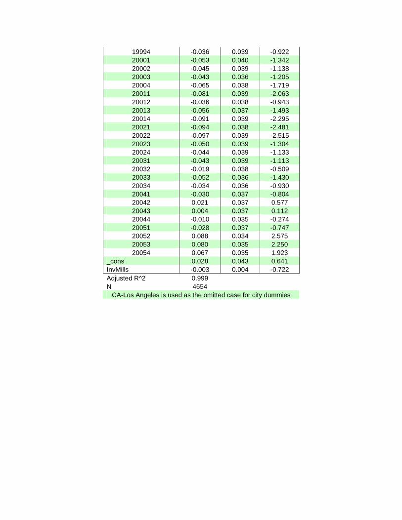
19994 -0.036 0.039 -0.922 20001 -0.053 0.040 -1.342 20002 -0.045 0.039 -1.138 20003 -0.043 0.036 -1.205 20004 -0.065 0.038 -1.719 20011 -0.081 0.039 -2.063 20012 -0.036 0.038 -0.943 20013 -0.056 0.037 -1.493 20014 -0.091 0.039 -2.295 20021 -0.094 0.038 -2.481 20022 -0.097 0.039 -2.515 20023 -0.050 0.039 -1.304 20024 -0.044 0.039 -1.133 20031 -0.043 0.039 -1.113 20032 -0.019 0.038 -0.509 20033 -0.052 0.036 -1.430 20034 -0.034 0.036 -0.930 20041 -0.030 0.037 -0.804 20042 0.021 0.037 0.577 20043 0.004 0.037 0.112 20044 -0.010 0.035 -0.274 20051 -0.028 0.037 -0.747 20052 0.088 0.034 2.575 20053 0.080 0.035 2.250 20054 0.067 0.035 1.923

_cons 0.028 0.043 0.641 InvMills -0.003 0.004 -0.722 Adjusted R^2 0.999 N 4654

CA-Los Angeles is used as the omitted case for city dummies

Heckman 1st Step: Selection Model

CoefficientStd.

Error t LogHedonic -0.369 0.015 -25.084 Other City -0.128 0.032 -4.02 IL-Chicago -0.111 0.039 -2.861 TX-Dallas -0.199 0.042 -4.733 DC-Washington 0.048 0.042 1.153 GA-Atlanta -0.172 0.043 -3.953 CA-Orange County -0.03 0.048 -0.63 CA-San Jose -0.093 0.054 -1.728 AZ-Phoenix -0.089 0.047 -1.879 TX-Houston -0.162 0.048 -3.346 MN-Minneapolis -0.151 0.05 -3.049 WA-Seattle -0.117 0.05 -2.337 CO-Denver -0.117 0.05 -2.337 MA-Boston -0.048 0.051 -0.945 CA-Oakland -0.169 0.056 -2.994 PA-Philadelphia -0.083 0.057 -1.464 CA-San Diego 0.045 0.056 0.808 MO-Saint Louis -0.138 0.061 -2.269 MD-Baltimore -0.019 0.059 -0.317 aptgard_dum -0.266 0.026 -10.307 apthigh_dum -0.149 0.059 -2.506 regionalmall_dum 0.059 0.072 0.817 retailmall_dum -0.071 0.062 -1.152 retailsingle_dum -0.55 0.05 -10.919 warehouse_dum -0.439 0.025 -17.926 indrd_dum -0.214 0.031 -6.944 indflex_dum -0.453 0.047 -9.664 offcbd_dum 0.012 0.034 0.357 offsub_dum -0.057 0.022 -2.615 sqft 0 0 -7.865 _cons -0.471 0.14 -3.377

19842 0.031 0.161 0.194 19843 0.464 0.142 3.266 19844 -0.128 0.174 -0.734 19851 -0.057 0.169 -0.336 19852 0.206 0.153 1.347 19853 0.319 0.147 2.175 19854 0.45 0.143 3.151 19861 0.025 0.164 0.153 19862 0.408 0.145 2.807 19863 0.295 0.149 1.978 19864 0.315 0.148 2.123 19871 0.185 0.154 1.201 19872 0.301 0.146 2.056 19873 0.259 0.148 1.746 19874 -0.06 0.166 -0.358

19881 0.172 0.152 1.135 19882 0.399 0.142 2.806 19883 0.37 0.142 2.598 19884 0.297 0.145 2.051 19891 0.171 0.15 1.137 19892 0.422 0.141 3.003 19893 0.537 0.137 3.906 19894 0.343 0.143 2.389 19901 0.101 0.154 0.657 19902 -0.151 0.171 -0.879 19903 0.474 0.138 3.425 19904 0.103 0.153 0.672 19911 0.509 0.138 3.685 19912 0.075 0.152 0.494 19913 0.006 0.156 0.036 19914 -0.134 0.164 -0.819 19921 -0.244 0.17 -1.437 19922 -0.128 0.156 -0.819 19923 0.274 0.138 1.983 19924 -0.098 0.154 -0.638 19931 0.074 0.146 0.505 19932 0.17 0.142 1.198 19933 0.304 0.138 2.201 19934 -0.024 0.149 -0.162 19941 0.104 0.144 0.723 19942 0.185 0.14 1.321 19943 0.418 0.134 3.107 19944 0.328 0.137 2.391 19951 0.284 0.139 2.047 19952 0.226 0.141 1.604 19953 0.323 0.138 2.342 19954 0.299 0.139 2.146 19961 0.33 0.138 2.385 19962 0.514 0.134 3.837 19963 0.804 0.129 6.211 19964 0.666 0.131 5.077 19971 0.62 0.132 4.689 19972 0.58 0.133 4.364 19973 0.815 0.13 6.284 19974 0.753 0.131 5.725 19981 0.568 0.136 4.175 19982 0.621 0.134 4.65 19983 0.906 0.129 6.998 19984 0.679 0.133 5.101 19991 0.773 0.131 5.881 19992 0.636 0.134 4.752 19993 0.752 0.132 5.711 19994 0.462 0.137 3.366 20001 0.424 0.137 3.083 20002 0.463 0.136 3.402

20003 0.85 0.13 6.559 20004 0.581 0.134 4.349 20011 0.432 0.137 3.16 20012 0.562 0.134 4.201 20013 0.639 0.131 4.861 20014 0.403 0.136 2.96 20021 0.567 0.133 4.277 20022 0.462 0.134 3.442 20023 0.782 0.137 5.724 20024 0.76 0.137 5.561 20031 0.451 0.134 3.363 20032 0.49 0.133 3.688 20033 0.663 0.129 5.126 20034 0.711 0.129 5.517 20041 0.59 0.131 4.516 20042 0.615 0.13 4.732 20043 0.61 0.13 4.7 20044 0.98 0.126 7.751 20051 0.573 0.131 4.384 20052 1.133 0.126 9.01 20053 0.888 0.128 6.948 20054 0.998 0.127 7.847

Pseudo R^2 0.05 N 142973

CA-Los Angeles is used as the omitted case for city dummies

A Simplified Transactions Based Index (TBI) for NCREIF Production

by

David Geltner

MIT Center for Real Estate & Geltner Associates LLC

May 2, 2011

Summary: This paper reviews the original TBI as it has been produced at MIT from 2006 through 2010, and explores a

simplified average-price-based alternative version for possible NCREIF production and publication, including

detailed operating instructions for such production.

The paper first briefly describes in relatively non-technical terms the nature and role of the “transactions based

index” (TBI) that the MIT Center for Real Estate, with NCREIF cooperation, has been producing and publishing

quarterly for five years based on sales of properties from the NCREIF Property Index (NPI) database. A transactions

based index such as the TBI is seen to be useful as a complement (not substitute) for the appraisal-based NPI. It is

noted that during the past five years the TBI has in fact gained a substantial user constituency in academia, industry,

and government.

In this paper a simplified methodology is proposed for producing a TBI without using regression analysis. The

simplified method is based on the average ratio each quarter of the sale price divided by the recent prior appraisal

for the properties sold from the NPI database. This index construction method can be implemented in Excel without

specialized statistical software or knowledge. This version of the TBI is more amenable to NCREIF production, and

may also appear more transparent to a non-academic practitioner community. It is therefore likely to be more

commensurate with ease of communication to industry researchers. In the present paper this simplified TBI is

labeled “NTBI”, for “NCREIF” version, to distinguish it from what is here labeled the “MTBI” for the pre-existing

“MIT” version.

This paper compares the recent historical results of the NTBI with the MTBI. It is found that the NTBI works well

and very closely replicates the MTBI at the aggregate all-property level. For producing sector level transactions

based indices (separate indices of apartment, industrial, office, and retail market segments, or conceivably other such

breakouts or sub-indices, such as geographic regions) it is recommended here that the transaction/appraisal

differences be based on the all-property sample of sold properties, pooled across all of the sectors. This differs from

the way the sector-level MTBI indices were produced. But in fact the MTBI sector indices have suffered from small

transaction samples, and the recommended NTBI sector index procedure here is based on the reasonable assumption

that transaction/appraisal differences do not tend to vary systematically across sectors.

The only major loss in a replacement of the MTBI by the proposed NTBI would be the Demand and Supply indices

that have been being produced at MIT, and that are based necessarily on regression models. These indices are

particularly useful for market diagnostic purposes, to quantify liquidity in the institutional property market, and to

provide a measure of “constant liquidity price movements” (in the case of the Demand Index). However, these

metrics have been primarily used by academics and in basic research and to date have found only limited use in

industry.

Considering the above, the author’s recommendation is that NCREIF should undertake regular quarterly production

and publication of what is here labeled the “NTBI” as an official NCREIF product (though for publication this could

simply continue the “TBI” label). In addition, it is the author’s suggestion that NCREIF allow occasional updates of

the of the Demand and Supply indices as they have been being produced at MIT, not as official NCREIF products,

but to serve special requests. It would be understood that any such production of TBI Demand and Supply index

updates must be produced by parties who have the capability to run the necessary regression-based models on their

own (with the necessary data supplied by NCREIF under confidentiality agreements), and explicitly without

NCREIF endorsement or confirmation.

Table of Contents:

1. Background …………………………………………. …Page 1

2. What is the TBI and Why is it useful? ………………… Page 2

3. How does the TBI work? ……………………………… Page 7

4. Addressing NCREIF’s requirements for TBI production:

A simplified TBI ………………………………… Page 9

5. Comparison of the NTBI and MTBI ………………….. Page 12

6. Conclusions & recommendations ……………………... Page 17

Appendix A:

Value-weighted &/or NOI-based versions

of the NTBI …………………………………….. Page A-1

Appendix B*:

Steps in the Operational Production

of the NTBI …………………………………….. Page B-1

(*Accompanied by a example Excel®

templates)

Page 1

A Simplified Transactions Based Index (TBI) for NCREIF Production

by David Geltner

1. Background

“In summary, we argue that the NCREIF Index is ready to evolve into two more specialized

successor families of index products: one tailored for fundamental asset class research support,

and the other tailored for investment performance evaluation benchmarking and performance

attribution.”

-- From: D.Geltner & D.Ling, Benchmarks & Index Needs in the U.S. Private Real Estate

Investment Industry: Trying to Close the Gap (A RERI Study for the Pension Real Estate

Association), October 17, 2000.

The National Association of Real Estate Investment Fiduciaries (NCREIF) is a non-profit industry

association founded in 1982 to serve the institutional real estate investment community as a non-partisan

collector, processor, validator and disseminator of real estate performance information. NCREIF’s

seminal information product is the NCREIF Property Index (NPI) which publishes quarterly investment

performance results for properties held on behalf of tax-exempt institutions by NCREIF’s data-

contributing members, which represent the majority of all major U.S. pension fund core real estate

investment holdings. The NPI has become a major reference and benchmark of U.S. real estate

investment performance and is widely cited and used in both academic and industry research.

An issue which has long been raised regarding some types of research is the fact that the NPI is based on

appraisals, or estimated valuations of its constituent properties as reported by the data-contributing

members. The quote at the top of this page is from a 2000 white paper commissioned by PREA which

suggested that, as valuable and relevant as the NPI is for many important types of analysis and research,

the industry could benefit from the development of complementary index products based more directly

and purely on realized transaction prices of properties sold in the marketplace.

With this in mind, the MIT Center for Real Estate proposed to NCREIF in 2004, and NCREIF

supported, the development of a “transactions based index” (TBI), based on the actual transaction prices

of the properties sold from the NPI database. Over the course of 2004 and 2005 the TBI was developed

at MIT by a team led by David Geltner and Henry Pollakowski at MIT and Jeff Fisher at Indiana

University. The TBI methodology and initial index results were presented at several academic and

industry research gatherings during 2005 and 2006, and published in great detail in a 2007 article in one

of the top academic real estate journals (hereinafter referred to as “FGP2007”).1 At its annual fall

meeting in 2005 NCREIF approved the regular on-going quarterly production and publication of the TBI

by, and at, the MIT Center for Real Estate, with the proviso that the TBI was not to be labeled or

identified as an official NCREIF product. MIT launched the regular quarterly publication of the TBI in

February 2006 with the 4th

-quarter 2005 index results (and index history going back to 1984), and MIT

has published the TBI every quarter since then (now through 4Q2010).2

1 J.Fisher, D.Geltner, & H.Pollakowski, “A Quarterly Transactions-based Index of Institutional Real Estate Investment Performance and Movements in Supply and Demand”, Journal of Real Estate Finance & Economics (2007) 34:5-33. 2 The TBI has been published electronically, on the MIT/CRE website at: http://web.mit.edu/cre. Note that, like NCREIF, MIT has always clearly stated that the TBI is not an “MIT product”, and is not to be officially named or labeled as such. The MIT

Page 2

In the five years since the start of the TBI’s regular publication, the index has gradually gained an

important user constituency. The TBI is frequently cited in academic articles (as of late 2010 the

FGP2007 article had 39 citations in Google Scholar3) as well as in industry reports and white papers

4.

The Federal Reserve Board research staff employs the TBI in their quarterly update to the FOMC, and

both Bloomberg and the Federal Reserve Bank of St.Louis have requested redistribution rights for the

TBI.5 Ibbotson Associates regularly provides the TBI by request to selected clients.

Purpose of the present report:

With the above in mind, NCREIF is presently contemplating taking in-house the production and

publication of the TBI, as a NCREIF product. Correspondingly, MIT is looking forward to transferring

much or all of the TBI production and publication responsibilities to NCREIF. The purpose of the

present paper is to present some ideas and considerations to help facilitate this transition. In particular, a

simplified version of the TBI will be presented and proposed.

2. What is the TBI & Why is it Useful?

As it has been produced at MIT, the TBI is a set of related indices all using the same underlying

transaction price based methodology, as described in the FGP2007 article (available on the MIT/CRE

website). The TBI is produced at the “All-property” level, which aggregates all NCREIF sold properties

as if in a single population. The TBI has also been produced separately at the national sector level for

each of the four core commercial property usage type sectors: apartment, industrial, office and retail, in

each case based on independent separate (purely within-sector) populations. For each of these five

aggregations, the TBI product suite has included four indices: Price change (or capital return), Total

return (which includes income), Demand-side reservation price changes (referred to as the “Demand

Index” or “constant liquidity index”), and Supply-side reservation price changes (referred to as the

“Supply Index”). Thus, there are in all 20 indices (4 different indices each for the five different

aggregations including the four sectors and the all-property aggregate). Like the NPI, the TBI is a

quarterly index, updated at the end of each calendar quarter. The TBI has been considered preliminary

during the current calendar year until the final end-of-year update after which the index has been

“frozen” (not subject to any further changes).6

Center for Real Estate has always provided the TBI gratis and pro bono as a service to the academic and industry research communities. 3 As another indication, this article ranks 9th out of 141 articles published in the JREFE from 2006 through 2008 in the number of its subsequent citations (by other articles) within the Social Science Citation Index, the premier index of academic journals in the economics and finance field. This is a good measure of the relative influence of an article in the academic community. 4 A typical example is: G.MacKinnon, “REITs and Real Estate: Is There Room for Both in a Portfolio”, PREA Research Report, October 2010. 5 Rights which, through 2010, no one had authority to give. 6 This “freezing” of the TBI is done for convenience of users, including to give index levels a permanency as reference benchmarks for historical price levels. It is also done for consistency with the official NPI, which is also frozen. As a practical matter, the TBI has generally not experienced significant “backward adjustments”, or changes to its previously estimated history as new sales data is appended to the historical database each quarter. (The TBI is not a “repeat-sales” index, which is a type of price index construction methodology in which backward adjustments can be more of an issue.)

Page 3

To better appreciate what the TBI is and how it is useful in the context of the institutional real estate

investment industry that NCREIF serves, let us step back and survey broadly the types of indices that

can be constructed for tracking and quantifying the pricing and investment performance of commercial

properties in the U.S. As suggested in Exhibit 1, at a very broad-brush level one can distinguish two

major types of investment property asset price and/or return indices: appraisal-based and transactions-

based.7

Exhibit 1

Transactions-based & Appraisal-based Indices:

Appraisal-based indices like the NPI are the original and “classical” type of performance index in the

institutional real estate investment industry. They are uniquely useful by virtue of providing a complete

and auditable “census” of all of the properties in a given specifically identified population of interest

(e.g., NCREIF approximates the “universe” of all core properties held by or on behalf of major tax-

exempt institutions in the U.S., all the data-contributing members of NCREIF). Because of this, and

because the appraisals on which such indices are based correspond closely to how net asset value and

7 This ignores other types that are less relevant in the present context, such as REIT-based indices, and survey-based “notional” indices based on brokers’ opinions. The description of “Appraisal-based” indices in Exhibit 1 has in mind in particular the rigorous, auditable investment performance benchmarking oriented indices compiled from exhaustive sets of property investment database-contributing members’ valuation reports, such as that of NCREIF and the Investment Property Databank (IPD). Other types of what might be termed “expert estimation-based” indices are also possible, such as Green Street’s recent “GSA-CPPI”, but may differ in important ways from the traditional appraisal-based indices considered here.

Typology of Investment Property Indices

Appraisal-based:• Based on regular,

consistent appraisals

(internal, external subjective

estimates of values)

• Census (not sample) of

target population (universe)

• Auditable, corresponds to

mgr reports to clients

• Suitable for benchmarking

Transactions-based:• Based directly purely on

transaction prices of sold

properties (objective info, cash

changing hands)

• Sold properties are a sample

of underlying population

• Important for research (acad &

indust), not suitable for

benchmarking

Ad hoc

Statistical

Synchronous: All properties

appraised as of end

of each period (IPD)

Rolling: Props

appraised on rolling

or staggered basis,

some ea period (NPI)

Two types are complementary, not substitutes.

Page 4

investment performance is officially reported by funds and investment managers to their investors and

clients, appraisal-based indices are most appropriate as benchmarks for gauging and understanding

investment management performance, and for tracking at a broad level the fundamental property

valuations underlying the official “book value” or “carried value” of the institutional investor clients of

such investment managers.

However, appraisal-based indices tend to exhibit what researchers refer to as “smoothing” or “lag bias”.

By necessity and norms of practice, the property-level appraisal process that underlies appraisal-based

indices tends to be more conservative about recognizing value changes, and more “backward-looking”

for price discovery and documentation, than are the principal parties engaging in actual transactions.

Also, in some cases the appraisals (or valuation reports) used in the index are effectively not updated for

all properties as of the end of each period (i.e., the appraisals in the index are staggered or rolling in

time). The overall result is that appraisal-based indices tend to exhibit dampened market cycle amplitude

and/or lagged turning points in the cycle, as well as lower return volatility, compared to transactions-

based indices. This smoothing and lagging bias can be problematical for certain types of investment

industry research, including market tracking, trading strategies, portfolio analyses, and comparisons

across major investment asset classes (such as real estate, equities, and fixed income).8

There are also some important populations of commercial investment properties that are not regularly

appraised (e.g., the broad population of all U.S. institutional commercial property, beyond just that held

by NCREIF members, including properties held by REITs and properties collateralizing CMBS). For

such properties, appraisal-based indices are not possible, but transactions-based indices can and are

produced.9 Therefore, for apples-to-apples comparisons between NCREIF property performance and

such broader populations, a transactions-based index for NCREIF properties is useful in principle.

Transactions-based indices, if well constructed, can address many of the above-noted issues concerning

appraisal-based indices, and provide a different perspective more directly reflecting movements in the

pricing within the asset marketplace. Transactions based indices thereby can provide a very useful and

interesting complement to (but not substitute for) appraisal-based indices, in the context of NCREIF’s

mission. Transactions-based indices by definition are based directly and purely on actually

consummated property asset sale transactions. Apart from possible reporting or recording errors, they

are thus based on completely objective price information, rather than the more subjective and judgment-

based valuation estimates that underlie appraisal-based indices. Methodologically, transactions-based

indices are in principle completely replicable. Transactions based indices have the theoretical virtue of

being based on the actual timing and amount of cash changing hands in the free market, thereby obeying

8 For example, appraisal-based smoothing and lagging have the effect in classical mean-variance optimized portfolio allocation research of making the role of the private real estate asset class appear greater than it actually is in comparison with the other asset classes that do not suffer from appraisal smoothing effects, such as stocks and bonds. This undercuts the usefulness of appraisal-based real estate indices in mixed-asset investment analysis research and can undercut the credibility of real estate as a core institutional asset class. Technically, the problem is that the smoothing and lagging bias tends to reduce real estate’s apparent volatility and covariance with the other asset classes. 9 The initial example is the Moody’s/REAL Commercial Property Price Index (CPPI), a repeat-sales index based on the Real Capital Analytics Inc database of property sales over $2,500,000, based on methodology developed at the MIT Center for Real Estate, produced and published monthly since December 2006. A similar more recent such index is the CoStar Commercial Repeat-Sales Index (CCRSI), produced and published monthly by CoStar Group since August 2010.

Page 5

the classical dictum: “follow the cash.”10

Transactions prices, in contrast to appraisal-based valuations,

directly reflect the current equilibrium, such as it may be, between buyers and sellers in the asset market

at any given time. All of the above gives transactions-based indices a certain type of credibility and

meaningfulness both among academic economists and among many practitioners and policy makers.

Such credible price tracking information can be useful for the real estate investment industry, helping to

raise the credibility and depth of understanding of the industry among a broader constituency.

Transactions based indices are also a useful practical tool in conjunction with appraisal based indices, as

the transactions based indices tend to temporally lead the appraisal indices in the major price movements

or turning points. Transactions based indices therefore tend to be more predictive, and they reduce the

smoothing and lagging bias problem noted previously.

Types of Transactions-based Indices: Ad hoc vs Statistical…

With this in mind, let us continue our overview of index typology, now focusing within the world of

transactions-based indices. Here one can distinguish two major approaches to transactions-based index

construction, as indicated in Exhibit 2 (on the next page). Ad hoc price indices are based on simple

average price metrics, without use of econometric optimization techniques or explicit control for

differences among the properties transacting in one period compared to the next. Ad hoc transaction

price based indices have been around for a long time in the housing industry, such as the National

Association of Realtors Median Home Price Index. Similar such indices in commercial real estate tend

to be more recent and not as high profile or not regularly published, but are available from sources such

as Real Capital Analytics and CoStar (among others). But ad hoc price indices have more serious

problems for commercial real estate than for housing, because of the much greater degree of

heterogeneity across individual properties in the commercial market. This leads to a major apples-vs-

oranges problem in comparing the average prices of properties sold one period with the average prices

of properties sold the next period. If, for example, the average price per square-foot increases from one

period to the next, to what extent is that due to an actual increase in same-property (or “same-store”)

asset prices, or rather to some sort of “flight to quality” in which a larger proportion of “premium” assets

were sold during the second period? Such ad hoc indices also do not take advantage of the capabilities

of modern statistics and computational power to minimize error or noise in the price indices.11

10 Good transactions-based indices, like the TBI, strive to filter out from the index database deals that are not “arms length”, whose prices do not reflect free market exchange. 11 A major attempt to produce what would here be classified as an ad hoc transaction price based index of commercial property occurred in 2007 with the launch by Standard & Poor’s of their S&P/GRA Commercial Real Estate Index available for trading on the CME (ticker: SPCREX). This was a type of average price per square foot index that attempted to control for differences in property types trading from one period to the next, but in an ad hoc manner without use of formal regression models. The index folded at the end of 2008 after it failed to register a significant decline in prices during the market collapse of that year, and with no trading of the index taking place. A more recent index which is a bit hard to classify is the Green Street Commercial Property Price Index (GSA-CPPI, launched in 2009), which is based on Green Street’s value estimates of REIT-held properties (used to construct Green Street’s REIT NAV estimates). As the author understands this index, though Green Street states that transactions are considered in the GSA-CPPI’s computation, the GSA-CPPI attempts to represent a leading indicator of property price trends by including information gleaned from brokers and information about deals in the negotiation phase in addition to closed transactions. The exact index construction methodology is not clear, and it is not clear to what extent formal econometric models are employed. The GSA-CPPI is interesting, but seems to be clearly (and perhaps purposely) a subjective measure, at least in part, and in that sense more akin to an appraisal-based index than a pure transactions-based index, though a very different type of “appraisal” process than what underlies the NPI.

Page 6

Exhibit 2

For these reasons, most academics, and more recently some of the more sophisticated industry

researchers, advocate statistically rigorous, econometrically-based transactions price indices. Such

indices make use of statistical regression to estimate the changes in market prices from one period to the

next, with more explicit and effective controls for differences in the type and quality of properties

transacting in different periods. On the other hand, ad hoc indices can sometimes have an advantage

over statistical indices in that many industry practitioners lack familiarity or comfort with regression

models of property prices. The ad hoc indices may appear more transparent or easy to understand

without specialized expertise, in some cases.12

The TBI as it has been produced at MIT represents an econometrically rigorous statistical index, based

on all, and only, the properties sold each quarter from the NCREIF population of properties (that is, the

properties included within the NPI). As will be presented later in Section 4, this paper will propose a

simplified version of the TBI that might be classified as an ad hoc index by the criteria described in this

section. However, it will be shown that the proposed simplified methodology replicates extremely

closely the econometrically based TBI that has been being produced at MIT. Indeed, the simplified TBI

methodology proposed in this paper attempts to have “the best of both worlds”, by taking advantage of

NCREIF’s unique data advantages to produce an index that essentially reflects the rigor and purity of a

12 This is not necessarily always true, particular if one delves into the details of index production, and in any case may be a problem more of communication about index methodology than an inherent or irreducible problem of the index methodology itself. It is also the type of problem that tends to go away over time, as the industry gradually learns about the transactions based indices, which are a relatively new type of information product in commercial real estate.

Typology of Transactions-based Indices

Statistical:• Controlled for differences in

traded properties between

periods.

• “Optimized” according to

econometric principles

(minimize error)

Ad Hoc:• Not controlled for

differences in traded

properties betw periods.

• Not “optimized” according to

econometric principles

Median Price/SF

Mean Price/SF

Repeat-Sales

Regression

(same-property)

Hedonic

Regression

(representative

property)

Any of these may be either equal-wtd or value-wtd across observations:

(Equal-wtd generally superior from a statistical perspective.)

Page 7

statistical transactions based index while retaining the transparency and intuitive appeal of a simple ad

hoc type index, as we shall see in the next section.

3. How does the TBI work?

In this section we will review the way the TBI has been being produced at MIT so as to facilitate the

understanding of, and transition to, the simplified TBI production method being proposed in this paper.

As produced at MIT, the TBI is based on a statistical regression model of the transaction prices of the

NCREIF sold properties. This is known in the academic literature as a “hedonic” price model. It will be

useful to understand something about this methodology even if NCREIF will use a different

methodology going forward, as the TBI to date has been based on this price model and the proposed

simplified TBI in fact tracks the regression-based index extremely closely.

A hedonic price index controls for the differences between properties transacting in consecutive periods

of time by the use of “hedonic variables” in a regression model of property transaction prices. The

hedonic variables describe the essential price-determining characteristics of each property. In classical

academic hedonic price models the explanatory variables typically include parameters such as the size,

age, and location (e.g., neighborhood, or distance from CBD, or from airport, etc) of the property. The

regression’s estimated coefficients on the hedonic variables control for cross-sectional differences

which could affect prices among the properties in the transaction sample. If the hedonic variables are all

temporal constants (i.e., they don’t vary across time within a given property, e.g., property size), then the

price model will also include time dummy variables (i.e., set equal to one for the period when the

property transacts, zero otherwise). The coefficients on these time-dummy variables will then reflect the

longitudinal (i.e., across time) differences in prices, and it is these longitudinal differences that matter

for constructing the price index.

If some of the hedonic variables also vary across time (e.g., property age, or more to the point:

property’s current appraised value), then the price index must be constructed by defining a

“representative property” whose hedonic characteristics are used in the right-hand side of the equation.

The price index is then defined by the changes in the model’s predicted price for the representative

property each period. To reflect “same-property” (or “same-store”) asset price changes in the index such

as investors actually face, it is necessary to somehow reflect in the hedonic variables the aging of the

properties from one period to the next, so that the representative property reflected in the index ages

one-for-one with the passage of calendar time (this of course is the case in property appraisals as they

are updated for the same building over time).

A data challenge in constructing a hedonic transactions-based index is that it requires good and

consistent hedonic data on all the properties in the transaction sample, for all of the important hedonic

variables. This is often problematical for commercial property in the U.S. Another (related) problem is

the issue of defining an appropriate “specification” of the model, that is, which hedonic variables to use,

and how to use them (e.g., what functional form, for example, shall one consider building age as a linear

variable in years, or a quadratic variable in years and years-squared, or what?...) These challenges often

make it difficult to construct useful hedonic price indices of commercial property, particularly from a

practical perspective for industry usage as opposed to purely academic study.

Page 8

The TBI’s Advantage as a Hedonic Price Index:

Fortunately, the NCREIF Index database provides a unique way to get around this data limitation,

because the properties in the NPI are all subject to frequently updated appraisals that are generally of

high quality and largely consistently made. The recent appraised value (or, more exactly, the NCREIF

data-contributing member’s officially reported valuation as employed in the NPI) of each property just

prior to its sale can be employed as an excellent “catch-all” composite hedonic variable, for use on the

right-hand-side of the hedonic price model.13

The recent appraisals capture almost all of the cross-sectional dispersion in the price-determining

property characteristics across the properties that are sold in the NCREIF database. The recent appraisals

also capture most of the longitudinal variation in property values, as the appraisals are frequently

updated and do largely reflect the changes over time in the market value of the properties (as indicated

in the appraisal-based official NPI capital return index). The time-dummy variables in the TBI price

regression therefore don’t have to do as much “work” as typical time-dummy variables in a more

traditional academic hedonic price model. They don’t need to capture all of the longitudinal changes in

value, but rather only the relative difference between transaction prices and appraisals each period. They

thus reflect, and enable “correction” of, the effect of the previously noted smoothing and lagging bias in

the appraisals.

The TBI is then constructed essentially as indicated in Exhibit 3 (next page), as the percentage price

changes implied by the changes in the model’s predicted transaction price of the TBI’s representative

property each period. The representative property is constructed so that its appraised value each period

(which is an explanatory variable on the right-hand-side of the price regression equation) reflects the

appreciation returns in the appraisal-based NPI capital return index. The TBI’s predicted price for the

representative property thus reflects both the evolution of the appraised values in the NPI as well as the

model’s estimated time-dummy coefficients which reflect the relative differences each period between

the transaction prices of the NCREIF properties sold that period versus their recent appraised values.14

In essence, one can think of the TBI capital return each period as consisting of two additive components:

(1) The change in the Representative Property’s appraised value since the previous period (as reflected

in the NPI capital return index); plus (2) The change in the relative difference between the transaction

prices and the appraised values (reported two quarters earlier) between the previous period and the

current period (the difference in the hedonic price model’s time-dummy coefficients between the last

period and the current period). For example, suppose the appraisal-based NPI capital return in Quarter

“t” is 2%, and suppose in Quarter “t” transaction prices (of deals closed in Quarter “t”) average 5%

13 To be more precise, the TBI uses the NPI reported valuation two quarters prior to the sale, so as to insure independence between the appraisal and the subsequent transaction price. In many cases the data contributor knows of a forthcoming agreed transaction price, and simply reports that as the property valuation for the NPI in the current quarter of the sale transaction and often even in the prior quarter. This is a practice that is entirely proper for the NPI, but would inject a tautological element into the regression model of the price if we did not go back to an earlier valuation report. We find that two quarters prior to sale is sufficient. 14 The previously-noted two-quarter lag is also accounted for in the index construction. That is, the representative property’s “appraised value” reflects the NCREIF appreciation index two quarters earlier, as the model’s time-dummy variable coefficients reflect the differences between the current transactions (closings) prices and those properties’ appraised values two quarters prior.

Page 9

above the “t-2” appraisals of those same sold properties. Suppose further that in Quarter “t-1”

transaction prices averaged 4% above the “t-3” appraisals (for the “t-1” sold properties). Then the TBI

capital return for Quarter “t” would be (in essence): 2% + (5% - 4%) = 2%+1% = 3%.15

Exhibit 3

4. Addressing NCREIF’s Requirements for TBI Production: A Simplified TBI…

The focus of the present paper is to assist NCREIF in making the TBI an official NCREIF information

product, including NCREIF taking over responsibility for production and publication of the TBI. With

this in view, an important consideration is the methodological nature of the TBI. As it has been

produced at MIT, the TBI is based on an econometric model, the hedonic regression price model

described above. Yet NCREIF does not wish to take on the production and publication responsibility for

an index that has the level of statistical modeling involved in the pre-existing TBI, including in

particular the hedonic price regression model that is at the core of the TBI as it has been produced at

MIT.

This leads to the present proposal for a slightly different “TBI” based on a simplified methodology, in

effect, a type of average price index not relying on regression analysis. In essence the simplified

methodology being proposed is to compute the average each quarter of the ratio of the relative price

difference between the transaction price and the recent prior appraised (NPI-reported) valuation of the

sold properties each quarter, and then to apply this average ratio to the NPI capital return index level, to

15 This is a slight simplification, as the model actually contains some other explanatory variables and other features of the statistical regression system, and as a mathematical device the MIT TBI’s regression model works in logs. But the above numerical example captures the essence of how the TBI works, and also suggests intuitively why and how a simplified version of the TBI could work, as will be described in the next section.

HOW THE TBI AS PRODUCED AT MIT WORKS…Index returns are based on differences between periods in

the hedonic price model’s predicted price for the

“representative property”…

Rep Prop’s

Predicted

Sale Price= f( , ) Time

dummies

Rep Prop’s

NPI-reptd Val

^Price model’s estimated

coefficients each period.

All set = 1 every

period to

capture

trans – apprsl

differ ea period.

Rep Prop’s NPI-reptd Val ea period = NPI avg

prop val @ index inception (1984) grown at

NPI capital appreciation rate (EWCF) since

then. Reflects evolution of appraised values

as in official NPI.

Page 10

“convert” it to a transaction price based version. Such a procedure might be labeled as “ad hoc”

according to the earlier discussion of transaction based index methodologies in Section 2. While it was

suggested there that in general there can be problems with such methodology for commercial property

price indices, we shall see in this section that a NCREIF-based average price index in the spirit of the

TBI can be quite effective, essentially just as effective as the econometric based TBI that has been being

published at MIT.

Why an Average-Price-Based TBI could work well for NCREIF:

The reason why a simple average-price based index can work well in the NCREIF context is

fundamentally the same reason that we noted earlier as to why the TBI’s hedonic price regression model

is able to avoid the major data challenge that faces most commercial property hedonic price indices.

This reason is NCREIF’s unique database of high quality, frequently-updated, consistent appraisals of

all the properties in the NCREIF population. These appraisals serve as the major right-hand-side

explanatory variable in the TBI regression model of transaction prices, by capturing most of the cross-

sectional and longitudinal dispersion in NCREIF property sales prices. In the TBI price regression, the

appraised value variable is the dominant explanatory variable, with a coefficient very near unity and a

standard error barely a percent or two (“t-statistic” in the 50 to 100 range or more), meaning that the

vast bulk of the price dispersion among NCREIF property sales is explained reliably and directly by the

appraised value.

Essentially, the only thing one has to do to create a good transaction price model of NCREIF property

sales is to estimate the relative difference (or ratio) between the sale price and the recent appraised value

among the properties selling within each period, and then multiply the average of these ratios each

period times the appraisal-based NPI appreciation index level to convert it to a transactions price based

index level each period (as suggested by the numerical example at the end of Section 3). In the existing

TBI as it has been produced at MIT the job of estimating the average difference between transaction

prices and appraised values each period is done in the hedonic price regression model by the time-

dummy variables. Those estimated differences are then applied to the index’s “representative property”

whose appraised value evolves exactly as the appraisal-based NPI capital index, to, in effect, “convert”

the NPI to the TBI.

But it is important to note that the basic statistical process that is used in the MIT TBI is what is known

as “Least Squares” regression (LS for short), which means that the computer calibrates the model by

picking coefficient values (on the explanatory variables, including the time-dummies) such that the sum

of the squared values of the “residuals” (the differences between the model’s predicted value of each

sold property and the actual selling price of each sold property) is minimized. In this process, by

construction, the sum of the (signed, not-squared) residuals becomes zero (as a mathematical by-product

of the minimization of the squared residuals). This means that the model’s average predicted sale price

exactly equals the actual average sale price among the NCREIF sold properties. This begs the question:

instead of using the regression model’s prediction of the average transaction price, why not just directly

use the actual average transaction price, as the basis for a “TBI”?

Thus, we may expect that we will get a very similar result to the TBI if we simply take the average sale

price among the sold properties each quarter and compare that to the recent prior average appraised

value of those properties, and apply that difference to the appraisal-based NPI appreciation index. In

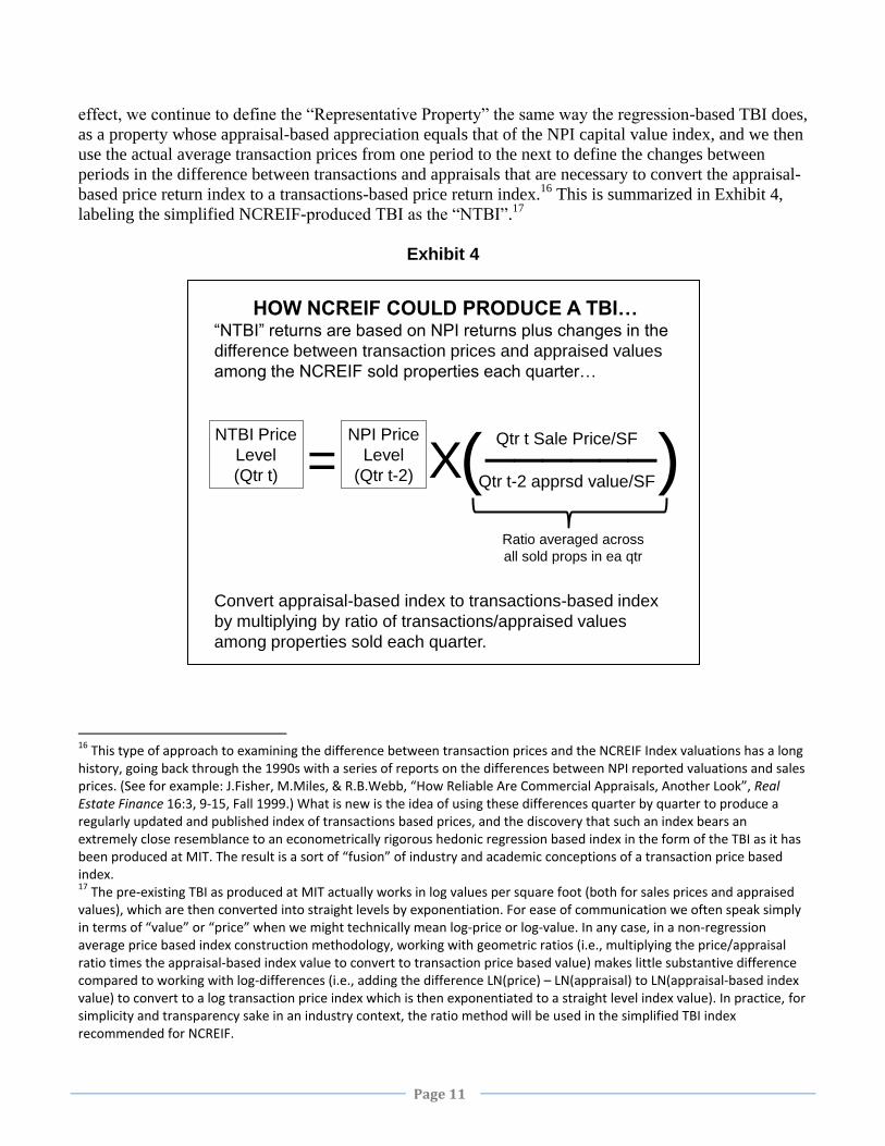
Page 11

effect, we continue to define the “Representative Property” the same way the regression-based TBI does,

as a property whose appraisal-based appreciation equals that of the NPI capital value index, and we then

use the actual average transaction prices from one period to the next to define the changes between

periods in the difference between transactions and appraisals that are necessary to convert the appraisal-

based price return index to a transactions-based price return index.16

This is summarized in Exhibit 4,

labeling the simplified NCREIF-produced TBI as the “NTBI”.17

Exhibit 4

16 This type of approach to examining the difference between transaction prices and the NCREIF Index valuations has a long history, going back through the 1990s with a series of reports on the differences between NPI reported valuations and sales prices. (See for example: J.Fisher, M.Miles, & R.B.Webb, “How Reliable Are Commercial Appraisals, Another Look”, Real Estate Finance 16:3, 9-15, Fall 1999.) What is new is the idea of using these differences quarter by quarter to produce a regularly updated and published index of transactions based prices, and the discovery that such an index bears an extremely close resemblance to an econometrically rigorous hedonic regression based index in the form of the TBI as it has been produced at MIT. The result is a sort of “fusion” of industry and academic conceptions of a transaction price based index. 17 The pre-existing TBI as produced at MIT actually works in log values per square foot (both for sales prices and appraised values), which are then converted into straight levels by exponentiation. For ease of communication we often speak simply in terms of “value” or “price” when we might technically mean log-price or log-value. In any case, in a non-regression average price based index construction methodology, working with geometric ratios (i.e., multiplying the price/appraisal ratio times the appraisal-based index value to convert to transaction price based value) makes little substantive difference compared to working with log-differences (i.e., adding the difference LN(price) – LN(appraisal) to LN(appraisal-based index value) to convert to a log transaction price index which is then exponentiated to a straight level index value). In practice, for simplicity and transparency sake in an industry context, the ratio method will be used in the simplified TBI index recommended for NCREIF.

HOW NCREIF COULD PRODUCE A TBI…“NTBI” returns are based on NPI returns plus changes in the

difference between transaction prices and appraised values

among the NCREIF sold properties each quarter…

NTBI Price

Level

(Qtr t) =NPI Price

Level

(Qtr t-2) XQtr t Sale Price/SF

(______Qtr t-2 apprsd value/SF)

Ratio averaged across

all sold props in ea qtr

Convert appraisal-based index to transactions-based index

by multiplying by ratio of transactions/appraised values

among properties sold each quarter.

Page 12

Terminology Note: “MTBI” & “NTBI”…

At this point it will be useful to establish some new terminology. Henceforth in this paper, unless it is

otherwise clear from the context, we will use the term “MTBI” to refer to the traditional regression-

based TBI developed and produced at MIT, and the term “NTBI” to refer to the non-regression-based

version based on average price relatives introduced here. If referring to issues that are in common with

both versions, we may simply use the term “TBI”.

5. Comparison of the MTBI & NTBI:

Exhibit 5 (on the next page) shows how well the expectation that the NTBI could produce index results

very similar to the MTBI is born out at the All-property level. The red line marked by diamonds traces

the NTBI over the past 10 years set to a value of 100 at the end of 2000. The blue line is the

corresponding MTBI.18

The black line is the corresponding NPI capital value index. From the evidence

in Exhibit 5 it would seem that there is very little difference, indeed no economically significant

difference, between the simple average price based NTBI and the more academic statistically based

MTBI, at the All-property level. Exhibit 6 then compares the NTBI to the MTBI at the sector level, and

here we see greater differences, which merit some discussion.

To begin, it is important to note that the primary focus of the development and publication of the TBI at

MIT has been at the all-property level. The TBI at MIT was a pioneering project, the first regularly-

published transactions-based price index of commercial property in the world, and as such it would

inevitably be a “learn as we go” project to some extent. This has been particularly true regarding the

sector indices.

The decision was made at the launch of the TBI in 2005 to produce the sector indices based only on the

sold property samples within each sector. In other words, each sector TBI as produced at MIT was

independent, based only on the properties sold within the subject sector. This seemed to make sense in

2005, when property transactions were plentiful. Even then, however, the scarcity of transaction

observations within each sector made it necessary to employ a special technique in the price regression

model at the sector level, known as a “ridge regression” noise filter. As transactions became

exceptionally scarce during the great downturn of 2008-09, the sector indices based only on their within-

sector sold-property samples seemed more problematical. This appears most notably in the case of the

Retail Index, which is the sector with the smallest number of property sales in NCREIF. In the quarterly

commentaries and FAQs-responses accompanying the MIT publication of the TBI updates, it was often

noted that users should be particularly cautious in using the sector level TBI indices, which it was noted

sometimes appeared inconsistent with the all-property results.

18 For an apples-apples comparison, both of the transactions-based indices are based on the same database, NCREIF’s “research” database as updated through 4Q2010. The version of the MTBI presented here is therefore “unfrozen”, reflecting any backward (historical) revisions based on this latest database. It therefore differs slightly from the “official” MTBI which as noted previously has been frozen at the end of each calendar year and until recently has not been based on the “research” database. (NCREIF’s “research” database differs from that on which the official NPI is based by including all revisions and additions into the history, whereas the official NPI has a frozen history.) In taking over production of the TBI, NCREIF may elect to officially retain the frozen history of the index as it has been published at MIT through 4Q2010, in which case the official NTBI history would differ slightly from what is depicted in Exhibit 5, in the same manner as noted above.

Page 13

Exhibit 5

Exhibit 6: Sector Indices Comparison of MTBI, NTBI, & NPI

90

100

110

120

130

140

150

160

170

180

190

20

00

4

20

01

2

20

01

4

20

02

2

20

02

4

20

03

2

20

03

4

20

04

2

20

04

4

20

05

2

20

05

4

20

06

2

20

06

4

20

07

2

20

07

4

20

08

2

20

08

4

20

09

2

20

09

4

20

10

2

20

10

4

MTBI, NTBI, & NPI Prices (4Q2010 data): 2001-2010 All-property

NPI EWCFset to

proper relationship in levels to NTBI(ratio)

MTBI (unfrozen) based on 4Q10data(set to

4Q00=100)

NTBI(ratio)set to 4Q00=100

90

100

110

120

130

140

150

160

170

180

190

200

20

00

4

20

01

2

20

01

4

20

02

2

20

02

4

20

03

2

20

03

4

20

04

2

20

04

4

20

05

2

20

05

4

20

06

2

20

06

4

20

07

2

20

07

4

20

08

2

20

08

4

20

09

2

20

09

4

20

10

2

20

10

4

MTBI, NTBI, & NPI Prices (4Q2010 data): 2001-2010 Apt-property

NPI EWCFset to proper relationship in levels to NTBI(ratio)

MTBI (unfrozen) based on 4Q10data(set to 4Q00=100

NTBI (ratio)set to 4Q00=100

90

100

110

120

130

140

150

160

170

180

190

200

20

00

4

20

01

2

20

01

4

20

02

2

20

02

4

20

03

2

20

03

4

20

04

2

20

04

4

20

05

2

20

05

4

20

06

2

20

06

4

20

07

2

20

07

4

20

08

2

20

08

4

20

09

2

20

09

4

20

10

2

20

10

4

MTBI, NTBI, & NPI Prices (4Q2010 data): 2001-2010 Industrial-property

NPI EWCFset to proper relationship in levels to NTBI(ratio)

MTBI (unfrozen) based on 4Q10data set to 4Q00=100

NTBI (ratio)set to 4Q00=100

90

100

110

120

130

140

150

160

170

180

190

2002

00

04

20

01

2

20

01

4

20

02

2

20

02

4

20

03

2

20

03

4

20

04

2

20

04

4

20

05

2

20

05

4

20

06

2

20

06

4

20

07

2

20

07

4

20

08

2

20

08

4

20

09

2

20

09

4

20

10

2

20

10

4

MTBI, NTBI, & NPI Prices (4Q2010 data): 2001-2010 Office-property

NPI EWCFset to proper relationship in levels to NTBI(ratio)

MTBI (unfrozen) based on 4Q10data(set to 4Q00=100

NTBI (ratio)set to 4Q00=100

90

100

110

120

130

140

150

160

170

180

190

200

20

00

4

20

01

2

20

01

4

20

02

2

20

02

4

20

03

2

20

03

4

20

04

2

20

04

4

20

05

2

20

05

4

20

06

2

20

06

4

20

07

2

20

07

4

20

08

2

20

08

4

20

09

2

20

09

4

20

10

2

20

10

4

MTBI, NTBI, & NPI Prices (4Q2010 data): 2001-2010 Retail-property

NPI EWCFset to proper relationship in levels to NTBI(ratio)

MTBI (unfrozen) based on 4Q10data(set to 4Q00=100

NTBI (ratio)set to 4Q00=100

Page 14

The transition of TBI production from MIT to NCREIF is an opportune time to revisit the methodology

underlying the sector level TBI indices, and in particular to reconsider the use of the independent within-

sector-only transaction samples. If we were to apply the above-described average-price-based “NTBI”

procedure independently within each sector, as the MTBI has been doing with the regression-based

index, we would obtain sector indices that would appear excessively noisy, even more so than the MTBI

sector indices shown in Exhibit 6. 19

Instead, we propose to base the average-price-based NTBI at the sector level on the all-property sold

property sample for the purpose of computing the average transaction price/appraisal ratio. In effect, we

propose basing the NTBI for sector indices or other such sub-indices on the assumption that the relative

difference between appraisals and transaction prices tends not to vary systematically across the property

sectors (or regions or any such breakout for which a sub-index would be produced). Under this

assumption, the pooled all-property transaction price sample is as valid for estimating the price/appraisal

ratio for any sector as it is for all sectors combined, and it therefore makes sense to use the largest-

possible sample to estimate the price/appraisal ratio for each sector, namely, the all-property aggregate

sample.

Thus, in the proposed NTBI represented by the red diamonds indices in Exhibit 6, we have applied the

same price/appraisal ratios to each of the sectors, ratios that are based on the larger all-property sold

property sample. The result is a set of NTBI sector indices that behave quite well, arguably better than

the MTBI sector indices, in terms of lack of excessive noise and in terms of movements in relation to

their corresponding appraisal-based NPI sector indices. The differences between the NTBI (red

diamonds) and MTBI (blue) indices at the sector level in Exhibit 6 is due largely to two factors: (1) the

use of the all-property transaction sample in the NTBI versus the sector-specific samples in the MTBI;

and (2) the use of the special ridge regression noise filter in the MTBI sector indices.20

19 The ridge regression noise filter is not possible in the simplified NTBI, and it has been that noise filter that has been largely responsible for keeping the MTBI sector indices from excessively noisy or wild-looking results. We should also note that the ridge regression noise filter was originally applied to the All-property index as well. At the all-property aggregate level the noise filter has no appreciable impact after the early years of the index, and has been dropped from the All-property index as it is currently produced at MIT. However, the early history of the All-property index would be considerably more noisy without that filter. This is one reason why NCREIF may want to retain the frozen MIT history for the All-property index. This is also why the sector indices only begin in 1994 instead of 1984 like the All-property index. 20 There are two other sources of the difference between the MTBI and NTBI at the sector level. One is that the regression-based MTBI is estimated on a pooled sample across the entire history of NCREIF transactions, and includes some additional explanatory variables which improve the price model’s fit at the individual transaction level but which are longitudinal constants and therefore have minimal impact on the index. Another source of difference is that the MTBI includes a special procedure to correct for “sample selection bias”, possible systematic differences between the properties that are sold and those that remain unsold in the database. This procedure, known as the “Heckman 2-stage” procedure has generally had only a very minor effect on the MTBI results. Analysis suggests that both of these differences account for only a small part of the empirical difference between the MTBI and NTBI apparent in Exhibit 6 in the Industrial, Office, and Retail indices. In the Apartment sector these other considerations appear to play a larger role, though the NTBI apartment index still appears superior to its MTBI counterpart (at least in relation to the NPI). Finally, note that the (relatively minor) differences across sectors in the relationship between the NTBI and its corresponding NPI are due purely to differences in the NPI sector indices appreciation between their 2-quarter-lagged values (to which the common all-property based price/appraisal ratio is applied) and their current values (with any such differences appearing on a rolling basis each quarter).

Page 15

Implications of the use of the all-property transaction sample at the sector level

While the assumption that transaction price/appraisal differences do not tend to vary systematically

across sectors is a reasonable working assumption, which appears to yield a useful set of sector or

regional sub-indices, it is of course only an approximation. It is important to keep in mind that this

assumption does have the effect of causing the contemporaneous correlation across the sectors (or

regions, across any breakout sub-indices) to appear larger than it otherwise would be. This is because

much of the quarterly volatility in the TBI derives from quarter-to-quarter changes in the transaction

price/appraisal ratio, and this ratio is being assumed to be the same across all the sectors or breakout

sub-indices within any given quarter. This “excess covariance” bias should be clearly noted on any

NCREIF publication of sector level NTBIs (or other breakout sub-indices), but it is not an issue with the

All-property Index.

Implications of the NTBI regarding Demand & Supply indices

The simplified average price based “NTBI” methodology will allow NCREIF to produce both price

index and total return index versions of the TBI.21

However, it will not enable production of the Demand

and Supply indices that have been part of the MTBI suite produced at MIT. The construction of the

demand and supply indices depends on the use of regression-based econometric modeling, including a

“probit” binary-choice model of property sales probability for the entire NPI population (unsold as well

as sold properties), in conjunction with the previously-described hedonic price regression model of the

sold properties. Of course NCREIF could certainly report simplified statistics about sales volume as a

fraction of NCREIF properties held each quarter, information that obviously speaks to the level of

liquidity in the NCREIF branch of the investment property marketplace. Such data about transaction

volume would be an excellent complement to the NTBI price index publication each quarter. However,

the econometric models are necessary to “convert” such volume-based measures into “price units” that

can be applied directly to price indices.

In other words, the MTBI Demand and Supply indices have enabled analysts to make statements such

as:

“Potential buyers reduced the prices they were willing to pay by X percent last quarter”

or:

“A combination of potential buyers raising their willingness-to-pay prices and potential

sellers, property owners, reducing their willingness-to-accept prices, by a total of X

percent as a fraction of the average current transaction price, will bring the marketplace

back to its long-term average level of liquidity or trading volume.”

Such integration of price and volume information about the market does not occur by merely publishing

volume information alongside transaction price information. The MTBI Demand Index in particular may

be interpreted as a type of “constant liquidity index,” tracing out the quarterly percentage changes in

potential buyers’ reservation prices which, if matched by sellers in actual deal prices, would keep the

21 See Appendix B and the Excel® example templates accompanying this white paper for details of NTBI production for both the price and total return indices.

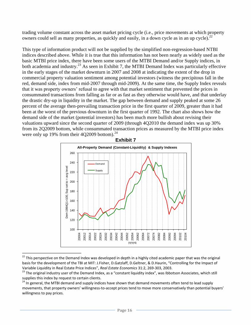
Page 16

trading volume constant across the asset market pricing cycle (i.e., price movements at which property

owners could sell as many properties, as quickly and easily, in a down cycle as in an up cycle).22

This type of information product will not be supplied by the simplified non-regression-based NTBI

indices described above. While it is true that this information has not been nearly as widely used as the

basic MTBI price index, there have been some users of the MTBI Demand and/or Supply indices, in

both academia and industry.23

As seen in Exhibit 7, the MTBI Demand Index was particularly effective

in the early stages of the market downturn in 2007 and 2008 at indicating the extent of the drop in

commercial property valuation sentiment among potential investors (witness the precipitous fall in the

red, demand side, index from mid-2007 through mid-2009). At the same time, the Supply Index reveals

that it was property owners’ refusal to agree with that market sentiment that prevented the prices in

consummated transactions from falling as far or as fast as they otherwise would have, and that underlay

the drastic dry-up in liquidity in the market. The gap between demand and supply peaked at some 26

percent of the average then-prevailing transaction price in the first quarter of 2009, greater than it had

been at the worst of the previous downturn in the first quarter of 1992. The chart also shows how the

demand side of the market (potential investors) has been much more bullish about revising their

valuations upward since the second quarter of 2009 (through 4Q2010 the demand index was up 30%

from its 2Q2009 bottom, while consummated transaction prices as measured by the MTBI price index

were only up 19% from their 4Q2009 bottom).24

Exhibit 7

22 This perspective on the Demand Index was developed in depth in a highly cited academic paper that was the original basis for the development of the TBI at MIT: J.Fisher, D.Gatzlaff, D.Geltner, & D.Haurin, “Controlling for the Impact of Variable Liquidity in Real Estate Price Indices”, Real Estate Economics 31:2, 269-303, 2003. 23 The original industry user of the Demand Index, as a “constant liquidity index”, was Ibbotson Associates, which still supplies this index by request to certain clients. 24 In general, the MTBI demand and supply indices have shown that demand movements often tend to lead supply movements, that property owners’ willingness-to-accept prices tend to move more conservatively than potential buyers’ willingness to pay prices.

100

120

140

160

180

200

220

240

260

20004

20012

20014

20022

20024

20032

20034

20042

20044

20052

20054

20062

20064

20072

20074

20082

20084

20092

20094

20102

20104

Dem

1984Q

1=100, S

up

set t

o =

avg

level

yyyyq

All-Property Demand (Constant-Liquidity) & Supply Indexes

Demand

Supply

Page 17

This type of perspective provides a unique real-time window into the functioning of the institutional

property market, with more depth than simple transaction prices alone, by drilling beneath those prices

into the two sides of the market that underlie the deals. This can be useful for diagnostic as well as basic

research purposes. It would seem sad to totally and forever remove from the information marketplace

the ability to access updates of these TBI Demand and Supply indices. For this reason, NCREIF may

want to remain receptive to future requests on the part of parties who have the capability to produce such

regression-based indices on their own, under suitable confidentiality restrictions and without NCREIF

assuming any responsibility for, or endorsement of, the product.

6. Conclusions & Recommendations Regarding the NTBI & MTBI

Based on the discussion and analysis presented in this paper, it seems eminently feasible for NCREIF to

take on production and publication of a “TBI” as an official NCREIF product and as a legacy of the

existing “MTBI” that has been being produced and published at the MIT Center for Real Estate. This

transition affords a good opportunity to make some changes in the TBI production methodology, and

this paper has presented and proposed such a change, in particular, a simpler, average price based

version of the TBI that does not require regression modeling. With this in mind, the following specific

recommendations are made.

1. NCREIF should move to adopt regular quarterly production and publication of a transactions

based index based on the simplified average price based methodology described in this white

paper (labeled herein as the “NTBI”, but for NCREIF publication purposes the acronym could

continue as simply the “TBI” that has gained fluency in the existing user community, i.e.,

without the “N”).

2. Sector level (or other such breakout) sub-indices of the NCREIF-produced TBI should be based

on the all-property average transaction price/appraisal ratio, applied in common to each breakout

sub-index, rather than being based on pure within-sector samples as the MTBI sector indices

have been. This recommendation is based on the plausible assumption that transaction/appraisal

ratios do not tend to differ systematically across sectors, and on the observation that using the

larger all-property sample for the sector indices seems to result in better sector-level TBIs.

3. Publication of any such TBI breakout sub-indices based on the all-property average

price/appraisal ratio should be accompanied by a “caveat” statement to the effect that cross-

correlations among breakout sub-indices may appear larger than they otherwise would as a result

of the all-property computation of the average price/appraisal differences.

4. It is recommended that in the interest of smooth transition NCREIF adopt the pre-existing frozen

history of the TBI as published at MIT through 4Q2010 in the case of the All-property aggregate

indices (both price and total return). However, due to the small-sample issues with the sector

indices as published at MIT, and in view of the more substantial change in the sector indices

reflecting recommendation (2) above, the NTBI sector indices should commence with new re-

stated histories going back to their (same) inception dates of 1Q1994; and finally…

Page 18

5. Regarding the Demand and Supply indices, NCREIF should continue to be receptive (as it has

been to the MIT Center for Real Estate) to parties appropriately requesting to, on their own, run

the Demand and Supply indices as these have been being produced at the MIT Center for Real

Estate as part of the TBI up until now, under suitable confidentiality restrictions, and under the

proviso that such Demand and Supply indices are not a “NCREIF product” and are not supported

or endorsed by NCREIF. Also, NCREIF should consider publishing transaction volume data

alongside the regular quarterly publication of the NTBI, including each quarter’s fraction of the

NCREIF stock sold that quarter (by count and by dollar volume). Such volume information is a

vital complement to pricing information to provide a current picture of the market.

A-1

Appendix A:

Value-weighted &/or NOI-based Versions of the NTBI

In defining the TBI representative property’s appraised value in constructing the price index, the

MTBI employs the equal-weighted/cash-flow based (EWCF) version of the NPI capital return

index, rather than NCREIF’s official value-weighted/NOI-based version (VWNOI) which is

represented by the NPI. There are two considerations underlying why the MTBI employs the

EWCF version of the NPI. One consideration is related to the “EW” (equal-weighted) issue, and

the other is related to the “CF” (cash-flow-based) issue. In both cases, this is a discretionary or

“policy” decision of the MTBI, and NCREIF could in principle elect to produce and publish an

alternative VWNOI-based version as the NTBI without violating any fundamental statistical

principles. This Appendix will review this policy question, and compare VWNOI-based and

EWCF-based versions of the NTBI at the All-property level.

Equal-weighted vs Value-weighted indices:

The MTBI has been using the EW version of the NPI to define the index’s representative

property because we view the TBI as a statistical inference device rather than a “universe” or

benchmark. In general statistical inference is more accurate when each observation is treated

equally.

One way to see this is to think of the principle of diversification of a portfolio. To take an

extreme example (which is correct for demonstrating the relevant point), a portfolio consisting of

100 nearly equal-sized assets will be more diversified (hence, have lower volatility) than a

portfolio containing 99 tiny assets and one gigantic asset whose value dominates the portfolio.25

This is why the equal-weighted version of the NPI tends to have lower volatility than the official

value-weighted version.

In the TBI’s original conception, before any other transactions based price indices of U.S.

commercial property existed (such as the Moody’s/REAL and CoStar indices today), we viewed

the TBI as representing the entire institutional U.S. investment property market, a larger

population than the NCREIF database. We were in effect viewing the NCREIF properties, and

the sold sample from them, as representing this broader population of properties. Treating the

TBI as representing a population broader than NCREIF meant treating NCREIF as a statistical

“sample” of this broader population, which in turn meant that one should use an equal-weighted

version of the NPI to represent the appraised value of the “representative property” used in

constructing the TBI.

This perspective changes a bit if one views the underlying population of properties represented

by the TBI as being not the broad U.S. institutional investment real estate market as a whole, but

just the specific properties held by NCREIF members and included in the NPI. Of course, the

TBI is still from this perspective a statistical inference, as most NCREIF properties are not sold

each period, and thus the sold properties represent a sample of the overall NCREIF property

population. Therefore the hedonic price regression model (or average price/appraisal ratio

25 This assumes the assets all have equal individual variance and pair-wise covariance.

A-2

estimate in the case of the NTBI) should still be based on equal-weighted data-points as before.26

But the NCREIF properties are now from this perspective no longer a sample but rather

constitute the entire population of interest. From this perspective it would be valid in principle to

apply the TBI’s estimate of transaction price/appraisal ratios to a representative property defined

(in terms of its appraised value) based on a value-weighted version of the appraisal-based

NCREIF Index.

Cash-flow based vs NOI-based capital return indices:

We now turn to the question of whether to base the TBI representative property’s appraised

value evolution on the “CF” or “NOI” definition of the capital return (aka “appreciation return”).

As is well known, investment periodic total returns (aka “simple holding period returns” –

HPRs), include two components: (1) the change in the asset (or static portfolio) value from

beginning to end of the period (calendar quarter in the case of the TBI); and (2) the net income or

cash flow generated by the asset (portfolio) for its investors during the period. The former

component is referred to as the “capital return” (or sometimes as the “appreciation return”, or the

“capital gain” or “growth component”). The latter component is referred to as the “income

return” (or sometimes the income or cash “yield”, or “current return”). The two components

should be defined in a non-overlapping manner so that their sum equals the “total return”

(sometimes referred to as “total yield”, or simply, the “yield”).

In the official NPI the capital return is defined for each property (and then aggregated up into the

index) as the change in the reported valuation of the property between the beginning and end of

the period minus any capital expenditures made on the property during the period. The official

NPI capital return thus reflects only the effect of the market for the asset (changes in its market

value) as well as the aging or “wasting” of the structure part of the asset, without reflecting how

the asset’s value may have been improved by capital expenditure investments made by the owner

into the property. Correspondingly, the official NPI income return is defined to equal the net

operating income (NOI) of the property without subtracting capital expenditures paid by the

property owner during the period. In other words, capex is not subtracted from the income return

even though it reduces the net cash paid out from the property to investors, and capex is

subtracted from the capital return causing that return to represent something less than the change

in property asset value from beginning to end of the period.

There is no doubt some rationale for this convention, and it is indeed common in many real

estate indices (e.g., IPD uses a similar convention). But the NPI properties exclude development

projects and major redevelopment or rehabilitation projects; so the vast majority of all the capital

expenditures in question are routine in the operation of the properties, and generally self-

26 A relevant limitation is the assumption, implicit in statistical inference, that the estimation sample is drawn from a single underlying population, as far as the parameters of interest are concerned. This can make the TBI non-representative for some segments of the property market if there arise market segments (possibly temporary) across which the relationship between transaction prices and appraisals differs sharply. For example, if larger properties systematically have a different transaction price/appraisal relationship than smaller properties. However, the solution to any such problem is probably not to value-weight the underlying data-points in the price/appraisal ratio estimation (given the small sold property sample size in any given period this would probably inject too much noise into the index). Rather, one would like to break the index into separate sub-indices corresponding to the different market segments, although again the small sold sample size might make this impractical.

A-3

financed from the operating revenues of the properties. As a result, the official NPI convention in

defining the breakout between capital and income returns can be somewhat “apples-vs-oranges”

and potentially misleading when comparing the NPI with stock and bond market based indices

(including REIT indices). In the stock market, for example, price or capital gain indices do not

subtract out the corporate capital expenditures made from earnings plowed back into the

company, and income returns are defined based on dividends, the cash actually paid out to

investors net of retained earnings held back in the company.

One of the major original motivations in developing the MTBI was to help provide the real estate

investment industry with a historical returns series that would facilitate apples-to-apples

comparisons between real estate and other asset classes (especially stocks and bonds). Therefore,

the policy decision was made a the inception of the MTBI to define its representative property’s

appraised value evolution based on the cash-flow based definition of the NPI capital return rather

than the official NOI-based definition. Another reason for this policy has to do with the other

transactions based price indices of commercial property which have been launched since the

TBI. Both the Moody’s/REAL CPPI and the CoStar CCRSI are repeat-sales indices which (like

the Case-Shiller and OFHEO repeat-sales housing price indices) do not subtract capex from the

price-changes tracked by those indices. Thus, for apples-to-apples comparison with the other

transactions based commercial property price indices, the TBI also needs to be based on the CF-

based definition of the NPI capital return. This makes the TBI a true price change index,

reflecting the changes in the average transaction price fetched by NCREIF sold properties from

one period to the next (on a “same-property” basis).

Summary:

In summary, the MTBI has by policy been based on the EWCF version of the NPI capital return

index. There are good reasons for this, in both the EW and CF considerations. However,

particularly given that there are now other commercial property transactions price based indices,

this is a policy decision that NCREIF might choose to revisit, if and to the extent that NCREIF

will launch its own “NTBI” version of the TBI. From a statistical perspective, it would be

possible to produce a VWNOI-based version of the NTBI, simply by applying the average

price/appraisal differences to the official VWNOI-based NPI capital return index rather than to

the EWCF-based version.27

Exhibit 8 (on the following page) provides a comparison of these two alternative approaches.

The top chart displays the NTBI capital value or price indices, together with their corresponding

versions of the NPI. The VWNOI-based versions, reflecting the official NPI capital growth index

in the NTBI’s representative property’s appraised value, show a markedly lower capital value

growth trend, due to the effect of subtracting capex out of the capital return component. The

bottom chart compares the equal-weighted vs value-weighed versions of the NTBI in the

cumulative total return indices. The equal-weighted index shows a slightly higher trend,

27 The Excel template provided with this white paper demonstrates exactly how to do this. Slight differences between the indices shown in Exhibit 8 and those in the Excel template reflect the fact that the indices in Exhibit 8 are based on log differences while the Excel template reflects ratio-based NTBIs.

A-4

indicating that on average in recent years smaller (lower-valued) properties held by NCREIF

members tend to have performed better than larger properties.28

Exhibit 8

28 It should also be noted that the VW index is based on the official NPI and therefore based on NCREIF’s “NPI” dataset of historical property returns, whereas the EW index is based on NCREIF’s “Research” dataset. The latter may have more backward-adjustments than the former, and this could also partially explain the difference between the two indices. Most of the differential trend in the total return indices is attributable to a few particular historical quarters: 2005Q4, 2006Q1, & 2006Q4.

90

100

110

120

130

140

150

160

170

180

190

20

00

4

20

01

2

20

01

4

20

02

2

20

02

4

20

03

2

20

03

4

20

04

2

20

04

4

20

05

2

20

05

4

20

06

2

20

06

4

20

07

2

20

07

4

20

08

2

20

08

4

20

09

2

20

09

4

20

10

2

20

10

4

NTBI & NPI Capital Value (4Q2010 data): 2001-2010 All-property: VWNOI vs EWCF

NPI VWNOI

NTBI VWNOI

NPI EWCF

NTBI EWCF

90

100

110

120

130

140

150

160

170

180

190

200

210

220

230

240

250

260

20

00

4

20

01

2

20

01

4

20

02

2

20

02

4

20

03

2

20

03

4

20

04

2

20

04

4

20

05

2

20

05

4

20

06

2

20

06

4

20

07

2

20

07

4

20

08

2

20

08

4

20

09

2

20

09

4

20

10

2

20

10

4

NTBI Total Return Index Equal-Wtd vs Value-Wtd: 2001-10 All-property

NTBI (VWNOI)

NTBI (EWCF)

B-1

Appendix B:

Steps in the Operational Production of the NTBI

See accompanying Excel example template

The primary rationale for the development of the simplified non-regression-based “NTBI”

version of the TBI is to facilitate NCREIF in-house production of the index. A related rationale

is to facilitate communication to and with the industry and practitioner community about the

NTBI, including the meaning and construction of the NTBI. In fact, the NTBI has been designed

to be able to be easily produced by NCREIF using only the existing NCREIF property database

and Excel®

.

An illustrative example of all of the steps in the production of the NTBI is contained in the Excel

workbook files that accompany the transmission of this report by the author to NCREIF. The

Excel workbooks start from the property-level NCREIF database and walk the reader through all

the steps of NTBI construction, including both capital (price) index and total return index, with

examples of both the All-property index and all four of the sector indices. The example

computations reflect the EWCF-based NTBI, but the All-property template also includes an

example of a VWNOI-based version. The Excel examples are fully annotated and documented,

and can serve as templates for actual NCREIF NTBI production. They are based on the actual

real world historical case of the 4Q2010 quarterly return computation and index update.29

Although the Excel example file is rather complete and self-explanatory, the essential production

steps will also be explicated here.

Computation of the NTBI price index:

There are two major phases in the NTBI price index construction: property level computations,

and index construction. We can divide the overall process into four major steps, which

correspond to the first four tabs in the example Excel workbooks (after the “readme”

introductory tab).

Step 1) Current Quarter Sold Property Compilation:

In this step the analyst compiles all of the properties that sold from the NPI database in the

current quarter (which we shall refer to generally as Quarter “t”). For conformity with the MTBI,

computations are based on values per square foot, and only on the core property types of:

apartment, industrial, office, and retail. Thus, we drop any observations that do not have a valid

square-foot entry or that are not among the four core property types.30

We also need to base the

29 In the case of the All-property NTBI, if NCREIF decides to retain the frozen MIT TBI history through 4Q2010, then the example in the template would be illustrative only, as the actual 4Q2010 result would be taken from the MTBI. This possibility is documented and treated in the template, which clarifies how the NTBI updating process would proceed from 1Q2011 onward. 30 This treatment of the square-foot variable could be re-examined by NCREIF. The division by square foot was originally adopted because it was contemplated to report the price model’s predictions in dollars per square foot rather than simply in an index of longitudinal percentage changes, and it was felt that price/SF would be more

B-2

appraisal value on the NPI reported valuation two quarters prior to the sale, so we must drop any

properties sold in Quarter t that don’t have valid square-foot and appraised (reported) valuations

in Quarter t-2.31

For the remaining valid, usable current-quarter sold property observations

(which is usually the vast majority of all the property sales out of the NPI in the current quarter),

you need to compile the sale price and the square-footage of each sold property.

Step 2) Lagged Two Quarters Data Compilation for Current Sold Properties:

In this step the analyst compiles the appraised (reported) valuation and the square-footage as of

Quarter t-2 for all of the properties sold in Quarter t. Generally this information would be derived

from the most recently updated historical dataset, the Quarter-t historical dataset, even though we

are pulling information about the properties as of two quarters earlier.

At this point it is important to verify that the valuation and square-footage information for

Quarter t-2 for all of the Quarter-t sold properties is consistent with the sale price and square

footage information for those properties as of Quarter t. For example, if a property had a partial

sale in Quarter t-2, and then the remainder of the property was sold in Quarter t, it might be

necessary to drop that observation from the index estimation dataset. The reason is that the

property as of Quarter t-2 before the partial sale may have been heterogeneous in terms of its

value per square foot. For example, the property might have included a retail component and an

office component, each with very different valuations per square foot. Supposing the retail

component was sold subsequent to Quarter t-2 but before the current quarter, the lagged

valuation per square foot would not be comparable to the current sale price per square foot.

Step 3) Computation of the Price/Appraisal Ratio for Quarter t:

The essence of the NTBI is to adjust the appraisal-based NPI by the average ratio each quarter of

the sold properties’ transaction prices divided by their recent (2-quarters prior) appraised (NPI-

reported) valuations (in each case adjusted by square-footage in the present model). Thus, we

compute the following ratio, which we’ll label “PriceOverAppr(i,t) for Property “i” sold in

Quarter-t. For each i = 1,2,…,N(t) of the Quarter-t sold properties:

PriceOverAppr(i,t) = (SalePrice(i,t)/SF(i,t)) / (ApprVal(i,t-2)/SF(i,t-2))

We then take the (unweighted) arithmetic average PriceOverAppr(t) across the N(t) properties

sold in Quarter-t:32

PriceOverAppr(t) = AVERAGEi[PriceOverAppr(i,t)]

intuitive and transparent than average price per sold property. However, this potential feature of the TBI was never implemented. 31 See explanation for this in footnotes in Section 3 of the main body of this paper. 32 If one wanted to construct a value-weighted estimate of the price/appraisal difference, you would first pool across all the sales within the quarter the sales prices and prior appraised values and square footage, and then perform the division and take logs on this pooled aggregate. As noted in Appendix A, this procedure risks any given quarter being overly dominated by one or a few large individual property sales, and this could add noise into the resulting TBI. It is also not necessary for deriving a “value weighted” TBI in the sense of using NCREIF’s population-based value-weighted NPI as the “representative property” to which the price/appraisal differences are applied to derive the TBI (as described in Appendix A).

B-3

Step 4) Construction of the NTBI Price Index for Quarter t:

We next want to use the PriceOverAppr(t) value we have just computed to “convert” the NPI

cumulative capital return index into the NTBI. We do this by first downloading the NPI capital

value index (levels) from the NCREIF database, and setting this index to have a value of unity

(or 100) in 1984Q1, the base period of the TBI.33

Include in the series all the accumulated capital

value levels starting two quarters prior to the TBI base period, so you will have a complete

quarterly history of the NPI capital values from 1983Q3 through the current quarter indexed to

1.00 (or 100) in 1984Q1.

We then multiply each of the quarterly value levels of the NPI capital index times the

price/appraisal ratio we just compute for the quarter two periods subsequent, for each quarter t =

1983Q3…current Quarter-t (or from 1993Q3 for the sector indices). This step is represented as

follows:

NTBI(t) = NPI(t-2)*PriceOverAppr(t)

In fact, the entire history of the NPI and TBI up until just prior to the current Quarter-t will

already have been computed and recorded the previous quarter (and initially MIT will transmit

this history to NCREIF), so the only change or updating that will be going on in this step is the

adding on the new current Quarter-t value.

The result is an NTBI capital value index that is indexed to an inception value of unity (1.00, or

100) as of 1984Q1 (or 1994Q1 for the sector indices). You can then compute the implied price-

change returns in the usual manner, for each Quarter “t”:

gNTBI,t = NTBI(t) / NTBI(t-1) – 1

Note that Step 4 can be applied either to the EWCF version of the NPI capital value index or the

VWNOI version, in exactly the same manner, depending on whether one wants the NTBI to be

based on the EWCF definition of capital (price change) returns or the VWNOI definition, as

discussed in Appendix A.

Computation of the total return index:

The above procedure describes how to construct the NTBI price index or capital value index.

The construction of the corresponding total return index is very similar, only with an extra step

to include the cash flow (or net operating income) component into the return, as demonstrated in

the previously-described Excel example file (see the worksheets in which the total return index is

computed). In brief, the procedure is as follows.

First, go back to the place in Step 4 where you had the NPI cumulative capital value index set to

a starting value of 1.00 (or 100) in 1984Q1. Think of these values as the value, in (say) hundreds

of dollars per square foot, of the NTBI’s “Representative Property” each period since 1984Q1.

Now fill in a new column with the corresponding income (cash flow or NOI, depending on

33 For the sector indices the base period is 1994Q1.

B-4

which form of NPI capital index you are using) in dollars per square foot, by multiplying the

previous quarter’s cumulative capital value level from the NPI (Representative Property

value/SF) times the NPI income return (either cash flow or NOI based) for the current quarter.

This computation may be expressed as follows:

CFNTBI,t = NPI(t-1)*yNPI,t

where “yNPI,t” is the NPI’s income return for Quarter t.34

Next, compute the NTBI total return in each Quarter t in the usual fashion employing the NTBI

capital value levels computed previously and the cash flow (or income) values derived just

above:35

1 + rNTBI,t = (NTBI(t) + CFNTBI,t ) / NTBI(t-1)

Finally, set the NTBI total return index to an inception value of 100 (or whatever value you

want) in 1984Q1, and grow it cumulatively forward by chain-linking in the usual manner:

NTBI_Total(t) = NTBI_Total(t-1) * (1 + rNTBI,t ).

34 We don’t need to “correct” cash flow or income information for transaction/appraisal differences, because presumably the cash flow and income information in the NPI is accurate and objective, not subject to appraisal or reporting effects. 35 We don’t need to explicitly employ the time-weighted denominator in this step because the NPI indices that underlie this computation already reflect such time-weighting.