a quaternion-based motion tracking and gesture...
TRANSCRIPT
A Quaternion-Based Motion Tracking and Gesture
Recognition System Using Wireless Inertial Sensors
by
Dennis Arsenault
A thesis submitted to the Faculty of Graduate and Postdoctoral
Affairs in partial fulfillment of the requirements for the degree of
Master of Applied Science
in
Human-Computer Interaction
Carleton University
Ottawa, Ontario
© 2014
Dennis Arsenault

ii
Abstract
This work examines the development of a unified motion tracking and gesture
recognition system that functions through worn inertial sensors. The system is comprised
of a total of ten wireless sensors and uses their quaternion output to map the player's
motions to an onscreen character in real-time. To demonstrate the capabilities of the
system, a simple virtual reality game was created. A hierarchical skeletal model was
implemented that allows players to navigate the virtual world without the need of a hand-
held controller. In addition to motion tracking, the system was also tested for its potential
for gesture recognition. A sensor on the right forearm was used to test six different
gestures, each with 500 training samples. Despite the widespread use of Hidden Markov
Models for recognition, our modified Markov Chain algorithm obtained higher average
accuracies at 95%, as well as faster computation times. This makes it an ideal candidate
for use in real time applications. Combining motion tracking and dynamic gesture
recognition into a single unified system is unique in the literature and comes at a time
when virtual reality and wearable computing are emerging in the marketplace.

iii
Acknowledgements
I would like to thank my supervisor, Anthony Whitehead, for providing me with this
opportunity and his guidance throughout this experience. I would also like to
acknowledge all of my comrades in the office who both helped me to accomplish my
work, as well as distracted me from it when needed. Of course I would also like to
acknowledge the support my friends and family have provided me throughout this time,
helping me to reach my goals.

iv
Table of Contents
Abstract .............................................................................................................................. ii
Acknowledgements .......................................................................................................... iii
Table of Contents ............................................................................................................. iv
List of Tables .................................................................................................................. viii
List of Figures ................................................................................................................... ix
1 Chapter: Introduction ................................................................................................ 1
1.1 Wearable Computing ...................................................................................................... 1
1.2 Motion Gaming .............................................................................................................. 2
1.3 Virtual and Augmented Reality ...................................................................................... 4
1.4 Gestures .......................................................................................................................... 5
1.5 Thesis Overview ............................................................................................................. 6
1.6 Contributions .................................................................................................................. 7
2 Chapter: Background ................................................................................................. 9
2.1 Body Area Sensor Networks .......................................................................................... 9
2.2 Body Area Sensors ....................................................................................................... 10
2.2.1 Physiological Sensors ............................................................................................... 10
2.2.2 Biomechanical Sensors ............................................................................................ 12
2.3 Body Area Sensor Network Applications .................................................................... 13
3 Chapter: Related Works .......................................................................................... 15
3.1 Active Games ............................................................................................................... 15
3.1.1 Dance Games ........................................................................................................... 15
3.1.2 Non-Dance Games ................................................................................................... 16
3.2 Motion Tracking ........................................................................................................... 17
v
3.3 Gesture Recognition ..................................................................................................... 20
3.3.1 Non-Markov Models ................................................................................................ 21
3.3.2 Hidden Markov Models ........................................................................................... 21
4 Chapter: The Sensors ............................................................................................... 23
4.1 Sensor Characteristics .................................................................................................. 23
4.2 Sensor Fusion ............................................................................................................... 24
4.3 Sensor Drift .................................................................................................................. 25
4.4 Quaternions................................................................................................................... 28
5 Chapter: Inertial Motion Tracking ......................................................................... 31
5.1 Sensor Placement .......................................................................................................... 31
5.2 Bone Orientation Mapping ........................................................................................... 33
5.3 Coordinate System Transfer ......................................................................................... 34
5.4 Initial Quaternion Offset ............................................................................................... 35
5.5 Calibration .................................................................................................................... 38
5.6 Orientation Overview ................................................................................................... 42
5.7 Skeletal Model .............................................................................................................. 44
5.7.1 Bone Base and Tip Positions .................................................................................... 44
5.7.2 Skeletal Walking Design .......................................................................................... 45
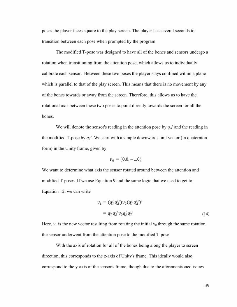
5.8 Game Design ................................................................................................................ 47
5.9 Oculus Rift Integration ................................................................................................. 49
5.10 Limitations and Issues .................................................................................................. 51
6 Chapter: Gesture Recognition ................................................................................. 54
6.1 Hidden Markov Model Theory ..................................................................................... 54
6.2 State Divisions .............................................................................................................. 55
6.3 The Gestures ................................................................................................................. 59

vi
6.4 Methods ........................................................................................................................ 60
6.5 HMM Testing ............................................................................................................... 61
6.6 HMM Results ............................................................................................................... 62
6.7 Markov Chain ............................................................................................................... 66
6.8 Markov Chain Results .................................................................................................. 67
6.9 Recognition Time ......................................................................................................... 71
6.10 Modified Markov Chain ............................................................................................... 72
6.11 Modified Markov Chain Results .................................................................................. 75
7 Chapter: Discussion .................................................................................................. 79
7.1 Motion Tracking Performance ...................................................................................... 79
7.2 Sensor Drift .................................................................................................................. 80
7.3 System Scalability ........................................................................................................ 81
7.4 Gesture Accuracy ......................................................................................................... 81
7.5 Multiple Gesture Recognition Sensors ......................................................................... 82
7.6 Number of Gestures ...................................................................................................... 83
7.7 Gesture Segmentation ................................................................................................... 83
7.8 System Unification ....................................................................................................... 84
8 Chapter: Conclusions ............................................................................................... 86
8.1 Thesis Findings ............................................................................................................. 86
8.2 Applications .................................................................................................................. 87
8.3 Limitations and Future Work ....................................................................................... 88
Appendices ....................................................................................................................... 90
Appendix A Confusion Matrices ............................................................................................... 90
A.1 HMM User Included ................................................................................................ 90
A.2 HMM User Excluded ............................................................................................... 92

vii
A.3 Markov Chain User Included ................................................................................... 94
A.4 Markov Chain User Excluded .................................................................................. 96
A.5 Modified Markov Chain User Included ................................................................... 98
A.6 Modified Markov Chain User Excluded ................................................................ 100
Bibliography and References ....................................................................................... 103

viii
List of Tables
Table 1. Results of multiplication of the quaternion basis vectors 28
Table 2. Total number of states for a given value of sectors (L) per π radians, and angle of
rotation spanned by a sector. 58
Table 3. Confusion matrix for the user excluded HMM case with four sectors per π
radians. 65
Table 4. Confusion matrix for the user included HMM case with five sectors per π
radians. 66
Table 5. Confusion matrix for the UI case with the MC algorithm at 3 sector values 70
Table 6. Confusion matrix for the UE case with the MC algorithm at 3 sector values 70
Table 7. Confusion matrix for the Modified Markov Chain for the UI case at seven
sectors 77
Table 8. Confusion matrix for the Modified Markov Chain for the EU case with seven
sectors 78

ix
List of Figures
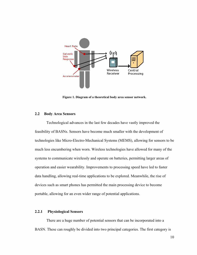
Figure 1. Diagram of a theoretical body area sensor network. ......................................... 10
Figure 2. The directions the sensor generates its global x and y axes. ............................. 24
Figure 3. Plot of the sensor's drift about the vertical axis over time under three different
conditions. ......................................................................................................................... 26
Figure 4. Magnified view of the first two minutes of sensor drift, highlighting the sudden
change after 13 seconds when device is stationary. .......................................................... 27
Figure 5. Image of a sensor in its 3D printed case with the Velcro strap. ........................ 31
Figure 6. Image showing the placement and operating channels of the sensors. ............. 32
Figure 7. Character model created in Blender for the motion tracking game. .................. 33
Figure 8. a) Orientation of the sensor on device startup with its generated global axis
frame. b) Sensor on the right upper arm with its generated global reference frame. c)
Charcter's arm orientation with Unity's axis frame. .......................................................... 34
Figure 9. Diagram showing the two poses used for performing the calibration routine. . 38
Figure 10. Diagram showing the rotation axis between the attention pose and T-pose in
both Unity's and sensor's reference frames. ...................................................................... 40
Figure 11. Images showing the gameplay area in Unity, as well as the character standing
in the middle of the room. The top image also shows the target in the distance. ............. 47
Figure 12. Image showing a user playing the game with the Oculus Rift. ....................... 51
Figure 13. Image of a user playing the game and shooting the target. ............................. 51
Figure 14. Showing the possible αstate values in blue for the different angles of α and
values of L......................................................................................................................... 57

x
Figure 15. Diagrams depicting the motion for each of the six gestures that were used. .. 60
Figure 16. Recognition accuracies for the different gestures using the HMM with a
varying number of sectors, under the user included condition. ........................................ 63
Figure 17. Recognition accuracies for the different gestures using the HMM with a
varying number of sectors, under the user excluded condition. ....................................... 63
Figure 18. Accuracy at each sector value averaged across all six gestures with the HMM.
........................................................................................................................................... 65
Figure 19. Recognition accuracies for the different gestures using the MC with a varying
number of sectors, under the user included condition. ..................................................... 67
Figure 20. Recognition accuracies for the different gestures using the MC with a varying
number of sectors, under the user excluded condition. ..................................................... 68
Figure 21. Averaged accuracy across all six gestures at each sector value for both the
HMM and MC................................................................................................................... 69
Figure 22. Average computation time for each model to parse and recognize a single test
sequence. ........................................................................................................................... 71
Figure 23. Accuracy results of the Modified Markov Chain for the user included case. . 75
Figure 24. Accuracy results for the Modified Markov chain for the user excluded case. 76
Figure 25. Accuracy results averaged across all gestures for the Modified Markov Chain
........................................................................................................................................... 77

xi

1
1 Chapter: Introduction
Since the early 1970's, when Xerox first began to include them in their personal
computers, the mouse and keyboard pairing has been the quintessential model for
interacting with computers [1]. While other interaction methods have come since then,
none posed any real competition to the mouse and keyboard dominated landscape. The
combination is extremely effective for a wide range of tasks and with all certainty will
not be disappearing from the computer environment anytime in the near future. However,
the mouse and keyboard are fairly restrictive in nature. This was previously of little
concern, as computers were so large that there was no alternative than to be confined to a
desk.
The last decade has seen a change in this paradigm. Ever increasing computing
power and decreasing size has led to computers we can carry in our pockets and that
outclass desktop computers from a decade ago. Under these much more mobile
environments the standard mouse and keyboard fail to perform well. This has led us to
explore new interaction modalities not possible a few decades ago.
1.1 Wearable Computing
The advent of a much more mobile and technology dominated world has given
credibility to the concepts of wearable and ubiquitous computing. This has led to a wide
range of ideas and innovations for marketable products. The Consumer Electronic Show
(CES) has seen an explosion of wearable computing devices in the last couple of years,

2
despite the fact that the market has not shown its complete willingness to adopt them yet
[2].
Despite this initial trepidation, the wearable device market is expected to exceed
six billion dollars by the year 2018 [3]. To date there has been some successes with
fitness wearables, however the potential scope of applications extends to encompass a
much wider range of uses. The proliferation of wearable devices has enabled further
exploration of body area sensor networks, which have been discussed in the literature for
several decades. Their potential uses vary greatly, including healthcare, training, and
security applications [4].
One area where wearables and body sensor networks might see early widespread
use is in the video game industry. While talking about brain-computer interfaces, Nijholt
et al. [5] suggest that video games make ideal testing grounds for newer technologies.
This is because the video game community is usually more accepting of new technology
and willing to overlook early issues and limitations.
1.2 Motion Gaming
Much like the mouse and keyboard, button and joystick based controllers have
always been the standard input modalities for gaming. But just as general computing has
seen new trends emerge in the last decade, so too has gaming. Nintendo has had massive
success with its Wii video game console [6]. It was the first widespread use of players
using their body motions to control a game, outside of select individual cases like Dance
Dance Revolution [7]. The Wii used a hand held controller that incorporated an
accelerometer, infrared sensor and gyroscope (in Wii Remote Plus) to track the motions

3
of the controller in the player's hand. Players were standing up and swinging their arms to
play tennis, rather than simply tapping a button while seated on the couch.
This brought to the forefront the idea of exergaming, the use of video games as a
form of exercise. There has been a steady increase in the prevalence of sedentary
lifestyles within the general population, which leads to various weight and health issues
including obesity and heart disease [8]. Exergaming is often seen as a way in which this
epidemic can be combated, by using the fun nature and growing popularity of video
games to generate player enthusiasm towards exercise.
The Wii unfortunately did not live up to this ideal, as players soon discovered that
they could perform just as well with simple wrist flicks instead of full body motions. This
quickly devolved to players again sitting on the couch and performing minimal motions
while playing. Despite this, recent works have shown that exergaming has promise and
can be an effective way to increase players' activity levels [9].
Not long after the Wii was released, Microsoft entered the market with the Kinect,
their camera based approach to motion gaming [10]. The Kinect system performed much
better than the Wii at generating an active aspect to gaming. Because the Kinect tracked
their full body, players were not able to cheat the system as easily as they could the
Nintendo Wii. However, the Kinect suffered from its own issues. Camera based systems
are very sensitive to lighting conditions, occlusion issues and play area restrictions. Since
the camera must be able to see the participant at all times the player must stay within a
very stringent play area. The Kinect also suffered from detection and latency errors,
which caused frustration among many players. Though the Kinect 2.0 version has

4
improved the accuracy and latency issues, the other problems are inherent to camera-
based technology and therefore much harder to avoid.
Wearable devices present new opportunities in the subject of gaming. Multiple
studies have explored the idea of incorporating heart rate [11][12][13] brain computer
interfaces [14][15][16] and other biological sensors [17][18] into games. Not as much has
been done using inertial sensors for body tracking, outside of simple handheld controllers
such as the Wii. Using inertial sensors could potentially outperform Kinect in full body
tracking applications. Inertial sensors would not suffer the occlusion, lighting and play
area restrictions that Kinect and other camera based systems have. They also have the
potential to obtain more accurate information on the player's pose than the simple camera
setups used for gaming. While there has not been a significant pursuit of worn inertial
sensors before now, that is quickly changing with the recent widespread development of
virtual and augmented reality technologies and the inclusion of sensors in wearables.
1.3 Virtual and Augmented Reality
Virtual and augmented reality has had a long history in science fiction. In reality
however, it has often been very disappointing. Oculus VR surprised many in 2012 when
it unveiled the development of its Rift product [19]. Their design allowed full 3D vision
and head tracking for gaming. While products like the Rift already existed, they were
very expensive and not aimed at a widespread consumer audience. Oculus VR attended
several conventions and released their development kits to the public, generating a high
level of interest. This was highlighted by their Kickstarter campaign that raised almost
2.5 million dollars [20]. While far from perfect, positive reactions to the capabilities of

5
the development kits reignited long held interest in the possibility of immersive virtual
reality.
This has led to interest in further developing motion controls, often with inertial
sensors, to allow for even more immersive experiences for the player. This is highlighted
by the very recent KickStarter project by Control VR [21]. It features inertial tracking
similar to the design described in Chapter 5 of this work.
While not specifically intended for gaming applications, Google also made a
foray into wearable technology with the announcement of its Google Glass [22]. The
device is worn like a pair of glasses, with a small screen above the right eye. The device
provides an augmented reality experience, with the ability to display information through
various apps, take pictures & video and allows for a wide range of voice commands.
1.4 Gestures
All of these applications move farther and farther away from the areas where the
mouse and keyboard excel. For these more mobile or active areas, alternative input and
interaction methods are required. Gestures are often seen as a solution to this problem.
While the rapid spread of touch screen phones has enabled the huge expansion of mobile
computing, it still requires the dedicated use of your hands for the interaction and
requires you to divert your attention to the screen. Worn inertial based gesture
recognition could allow for hands free interactions for a huge range of devices. Accessing
your mobile phone without taking it from your pocket, controlling augmented
applications like Google Glass, and controller-less virtual reality with the Oculus Rift all

6
present opportunities where gestures could make a significant contribution to the
interaction.
1.5 Thesis Overview
We will begin this thesis with a brief discussion on some background topics of
note. This includes an overview of body area sensor networks, different sensor types and
their basic functions, as well as a few applications that body area sensor networks are
well-suited for outside of the main active gaming focus of this thesis.
Chapter 3 then discusses works related to our own. This includes an examination
of other active games that have been created that focus on the use of inertial sensors as
one of their key components. Motion tracking with inertial sensors is also discussed as
well as related gesture recognition studies. Throughout this chapter we highlight any
studies that have strong connections to our own and highlight the similarities and
differences between these works.
Chapter 4 gives details about the sensors that were used throughout our
experiments and their characteristics. This section also gives a brief summary of the
mathematical properties of quaternions, to facilitate a better understanding of the
following chapters. We then proceed into Chapter 5, where we outline the process of
mapping the motions of a user to those of an onscreen character using the quaternion data
obtained from the worn sensors. This involves a wide range of sections covering such
topics as the basic bone mapping, coordinate transformations, calibration routine and the
skeletal model used for character movements. This chapter concludes with a discussion

7
of a game created to demonstrate the capabilities and strengths of our motion tracking
system.
Chapter 6 focuses on the use of the sensors for gesture recognition. We begin by
outlining some of the basic theory behind the recognition algorithms before advancing
into the specifics of our methods. The design of our experiments is outlined and the
results for the Hidden Markov, Markov Chain and Modified Markov Chain are
successively examined and compared.
Chapter 7 discusses the results of the motion tracking and gesture recognition
systems in more depth. Their current weaknesses and areas for future work are
considered both individually as well as how the two systems fit together. Finally, the
findings of the thesis are summarized and its contributions reiterated in Chapter 8.
1.6 Contributions
While inertial sensors do have some presence in the current literature surrounding
motion capture in gaming, few works involve the inclusion of the full body. Our system
allows player motions to be mapped to those of their on-screen character in real time. The
system functions entirely off of quaternion orientation data transmitted from the body
worn sensors. A simple way to calibrate the orientation of the sensors based on their
quaternion output is presented, as well as a hierarchical skeletal model. This skeletal
model allows for very easy and natural navigation by the user around the virtual
environment by placing the character's anchor point on the planted foot rather than the
torso, as in other systems [23]. The game we created highlights the strengths of the
system's design as well as its potential for virtual reality applications.

8
We also examine the system for its capabilities in performing quaternion based
gesture recognition. The goal is to have a unified motion tracking and gesture recognition
system. To date, these two concepts have only ever been examined exclusively, rather
than in a combined context. The quaternion based recognition algorithms we present are
based on Hidden Markov Models and Markov Chains. Despite the wide spread adoption
of the Hidden Markov Model in gesture recognition, our results found that our Modified
Markov Chain outperforms the Hidden Markov Model in both accuracy and computation
time.
The final design is a unified tracking and gesture recognition system for real time
applications. It also lends itself to easy scalability, depending on whether full body
tracking and recognition is needed or only certain key body parts. As all of the involved
sensors are worn, the interactions can be completed hands free and with the player's full
mobility. While the focus of this work is the system's use for gaming, the results are
easily extendable to other topics where body area sensor networks could be useful.
9
2 Chapter: Background
2.1 Body Area Sensor Networks
A body area sensor network (BASN) is a network of sensors that are used to
determine the current state, or changes of state, of an individual. The network is
comprised of various sensors that are typically worn on the body, though in special cases
they may also be implanted within the body. The type, distribution and number of sensors
included vary depending on the specific application requirements.
Each sensor in the network, sometimes referred to as a node, measures
information regarding a particular state of the wearer. This information may then be
passed on to a central transmitter also located on the body. This transmitter relays all of
the sensors' data to the main processing device. Depending on the design of the network
and sensors, this central transmitter may not be present, and instead each sensor will
transmit its own data to the receiver connected to the main processer. The latter situation
is the case with our experimental setup, where each sensor contains its own wireless
transmitter. The basic design of a theoretical BASN can be seen in Figure 1, which shows
the different components and how information is transferred. The main processing device
handles the principal calculations and manipulation of the data in accordance with the
needs of the application. For much more in depth discussions on BASNs and their
various components outside the scope of this writing, the reader can refer to [24] and [4].
10
Figure 1. Diagram of a theoretical body area sensor network.
2.2 Body Area Sensors
Technological advances in the last few decades have vastly improved the
feasibility of BASNs. Sensors have become much smaller with the development of
technologies like Micro-Electro-Mechanical Systems (MEMS), allowing for sensors to be
much less encumbering when worn. Wireless technologies have allowed for many of the
systems to communicate wirelessly and operate on batteries, permitting larger areas of
operation and easier wearability. Improvements to processing speed have led to faster
data handling, allowing real-time applications to be explored. Meanwhile, the rise of
devices such as smart phones has permitted the main processing device to become
portable, allowing for an even wider range of potential applications.
2.2.1 Physiological Sensors
There are a huge number of potential sensors that can be incorporated into a
BASN. These can roughly be divided into two principal categories. The first category is

11
physiological sensors, which detect the state of and changes in physiological properties.
While not exhaustive, examples of these include:
Heart Rate Sensor: Heart rate sensors detect a subject's heart rate in beats per minute, as
well as heart rate variability. This is accomplished through chest/wrist bands, finger clips
or electrodes. Heart rate is used to detect factors like exertion level [11][12], frustration
[25] and engagement in an activity [13].
Galvanic Skin Response Sensor (GSR): The electrical properties of the skin vary
depending on the sweat level and the associated eccrine glands [26]. These levels will
vary depending on an individual's level of stress or frustration. A galvanic skin sensor on
the finger or palm can be used to estimate the change in these emotional states [27][28].
Electromyography (EMG): When muscles contract they produce measurable electrical
potentials across the surface of the skin. These potentials can be measured by placing
electrodes on the skin's surface near the desired muscle. These sensors can be used for
measuring voluntary contractions for purposeful input, or involuntary contractions to
measure frustration or stress [25][17].
Brain Computer Interfaces (BCI): Similar to muscles, the brain gives off detectible
electrical signals while working. Systems that detect these signals using electrodes or
other techniques can be applied to record a wide range of signals for either explicit user
control [14][15][16] or simple detection purposes [29].
Respiration Sensor: Respiration sensors often make use of a chest band. The chest band
expands with the chest to measure both respiration rate as well as volume. These sensors
may be used for either a passive or active control scheme [17][18].
12
These different sensors measure physiological properties that the user may or may
not have conscious control over. They permit for a wide array of potential applications,
both in gaming as was discussed here, but also in medical applications where the
biological signals can be monitored and analyzed [30].
2.2.2 Biomechanical Sensors
The second category of body sensors are the biomechanical sensors, which are the
type of sensor that is used throughout this thesis. They are used to measure the physical
position and movements of an individual. Three of these sensors are of key significance
for this work:
Accelerometers: An accelerometer measures any acceleration that occurs along the
device's axis. Because of this, 3-axis accelerometers are often used to allow accelerations
to be measured in any direction. This is accomplished by placing three accelerometers in
an orthogonal configuration and is now a standard design in most modern accelerometers.
Accelerometers are able to provide information on their angle of inclination with respect
to the downwards direction by sensing the acceleration of gravity. Unfortunately they are
unable to distinguish between this gravitational force and actual accelerations [31]. While
double integration could theoretically be performed to obtain positional information, the
noise on the data makes this extremely difficult and imprecise, even with extensive
filtering [32].
Gyroscopes: While accelerometers detect linear accelerations, gyroscopes are used to
detect angular velocities. Unfortunately, gyroscopes lack the capability to determine their
absolute orientation. While accelerometers suffer most from noise in their readings, even
13
the best quality gyroscopes suffer from drift issues [32]. Drift results in small angular
velocities being reported even when the device is completely stationary. Over time this
drift will accumulate and can become a significant issue. Gyroscopes are especially adept
at accurately detecting quick rotations rather than long slow rotations.
Magnetometers: Magnetometers are sensitive to magnetic fields and are often used to
discern the direction of the Earth's local magnetic field. A magnetometer can use the
Earth's magnetic field as a reference direction in the same way an accelerometer uses the
directional force of gravity. The Earth's magnetic field is weak and can be easily
disrupted or overpowered by nearby metallic objects or electronics and so care must be
taken when using magnetometers [32].
When accelerometers, gyroscopes and magnetometers are used together they are
often collectively referred to as an inertial measurement unit (IMU). This is due to the
way in which they operate, by making use of the physical laws of mass and inertia to
determine their motions and orientation. Combining their output data to obtain a better
measure than any one individual sensor is the topic of sensor fusion and is discussed later
in Section 4.2.
2.3 Body Area Sensor Network Applications
All of these different sensors can be used in countless combinations, with the
sensors selected to best meet the needs of the application. Health care systems are being
examined as a very useful space for BASNs. They can allow for remote monitoring of
patients [30][33], fall detection in the elderly [34], and better physiotherapy treatments
[35]. Some military applications are being examined [36][37], as well as professional

14
sports training [38], general exercise promotion [39][40][41], and security authentication
and information sharing [4]. In this work we choose to design our system around an
entertainment and gaming application. However, our methods and findings are equally
applicable to any of the other areas where BASNs may be useful.

15
3 Chapter: Related Works
3.1 Active Games
There are currently very few studies that have looked at using IMU sensors as the
primary mode of interaction for gaming. Some commercial products like the Nintendo
Wii and Playstation Move make use of IMU sensors for gameplay, but only through
hand-held controllers that include multiple buttons. There is currently a growing
epidemic of sedentary lifestyles leading to weight gain and health problems [8].
Exergaming, the use of video games to promote exercise, is a rapidly growing field and
has already been shown to be effective at increasing physical activity [9]. Exergames are
specifically aimed at getting the player to exercise, while active games are not as heavily
focused on meeting exercise requirements. Active games still aim to be physically
involving, but are not created with the goal of generating a physical workout for the
player. Despite these slightly different goals, both styles could benefit greatly from
BASNs and IMUs by freeing players from handheld controllers.
3.1.1 Dance Games
The sensor network for active play (SNAP) system made use of four
accelerometers located on the wrists and knees to determine a player's pose [31][42][43].
Incorporating the whole body in this way allowed them to avoid the cheating issues seen
with the Wii, where players can simulate full body motions with simple wrist flicks. The
SNAP system could sense the inclination angle of the four accelerometers. By comparing
these readings to previously trained reference poses, the system could determine if a

16
player was matching the desired pose. A few different games were devised for the
system, however all focused around dancing as their central premise.
Dance games are one of the most popular types of active game, both in research
and commercially. In [44], Charbonneau et al. argue that dance game popularity stems
from the low barrier to entry and most people's willingness to try them. Their work
follows closely to that of the SNAP system. They created their own version of a dance
game using four worn Wiimotes on the ankles and wrists. Other dance based games have
also made use of IMU sensors in some capacity, such as in [45] and [46].
These dancing works are entirely based on either static poses or characteristic
signals. This means that they detect if a player is in a given predefined pose at a certain
instance or look for a specific signal, like a rapid acceleration in a particular direction.
They do not function on a continuous basis, which involves tracking the player's motions
over time. Since the player is supposed to make a certain pose in beat with the music, the
dancing program must only check that they are in that particular pose at a specific
moment in time. This is significantly easier than determining what action or gesture a
player performed at any given time from a multitude of possible options.
3.1.2 Non-Dance Games
There have been some non-dance-based games developed that use worn IMUs as
well. Wu et al. [47] created a virtual game of Quidditch, a sport from the Harry Potter
universe. They used two IMU sensors on the player's arm, as well as one on both their
prop broom and club. The player steered by moving their held broomstick and used their
arm and club to attack incoming balls. To increase immersion the setup used multiple

17
screens to project the view on multiple sides of the player. However, they do not give
many specific details on the sensor based interactions or gameplay.
Both Zintus-art et al. [48] and Mortazovi et al. [49] created games that use a
single sensor attached to the player's ear or foot respectively. In [48] they used an
accelerometer to determine if the player was running, walking, jumping, or leaning.
These actions controlled an on-screen dog character and the player's goal was to avoid
oncoming obstacles. Though a very simple setup, they achieved very high recognition
accuracy results at almost 99%, with recognition times under a second. Meanwhile, [49]
used an accelerometer and pressure sensor combination to control actions in a soccer
game. Though the player still made use of a standard controller for some inputs, the worn
sensor was involved in the running, passing and shooting actions. They also put
significant consideration into protecting the system from being cheated in the same way
as the Wii.
These works are still far from tracking full body poses and motions. They all use a
low number of sensors, giving them a limited amount of information on the player. While
their motion/action recognition methods are suitable and perform well for the
requirements of their designed games, they likely would not scale well for much more
complex applications than what they have presented.
3.2 Motion Tracking
Outside of the entertainment space there have been several papers examining the
prospect of more detailed motion and position tracking of an individual through the use
of worn IMU sensors. Previously, body motion tracking has been primarily accomplished
18
through optical means due to its high level of precision. This has been further bolstered
by the development of Microsoft's Kinect system. Though the Kinect lacks the precision
of advanced multi-camera systems, it allows for easy motion tracking at a more
economical cost. These optical systems have major limitations though, as they require
constant line of sight of the subject and self-occlusion can be problematic. Camera-based
systems also suffer when there are poor lighting conditions and require the user to stay
within a very stringent operational area.
Motion tracking with IMU sensors is becoming more feasible for the same
reasons as BASNs. Elaborate and precise camera setups are very expensive and similar
accuracies could potentially be achieved using a distributed network of IMU sensors
across the body. While IMU systems do not currently perform at the same level of
precision as optical systems [50], there are many situations where they could still thrive.
They may be beneficial where extremely high levels of precision are not required, where
cost is a major factor (such as in consumer products), or where the limitations of a
camera system are major concerns.
The motion capture with accelerometers (MOCA) system [51] used
accelerometers to detect arm inclination and also made use of very simple gesture
recognition. The system comprised only a single accelerometer and their gesture
recognition was based on the current inclination angle rather than dynamic motion-based
gestures. They used this recognition to allow users to navigate a virtual world using their
wrist orientation.
Zhang et al. [52][53] tracked arm motions using a pair of sensors containing an
accelerometer, gyroscope and magnetometer on the upper arm and forearm. In addition to

19
determining the orientation of the arm through their sensor fusion algorithm and
unscented Kalman filter, they also imposed geometrical constraints on the system. These
involved biomechanical factors such as the lack of adduction/abduction movement in the
elbow. This helped them to constrain noise and estimation errors in their readings. Their
results were very successful compared to the accuracy of an optical tracking system.
Similar IMU tracking experiments were also conducted in both [54] and [55].
Full body tracking suits were proposed in [56] and [57], with multiple sensors
positioned at various points across the body. The former work tested a single instance of
their iNEMO sensors, comprised of an accelerometer, gyroscope and magnetometer,
against commercial inertial sensors like those by Xsens [58]. Though the iNEMO sensor
had lower precision, it still performed well for a significantly smaller cost investment.
iNEMO M1 sensors were then used to build a partial full-body tracking suit in [23]. Five
sensors were used to track the orientations of the forearm, upper arm, torso, thigh and
shin on the right side of the user's body. Their system recorded the orientation of these
limbs and displayed them on a skeletal model in real time.
While this system operates similarly to the one we developed, there are several
important differences. We expand the sensor network to include the full body using ten
sensors, rather than only the right side with five sensors. In Section 5.5 we detail an
alternative, easy-to-perform method of calibration to determine the user's reference
frame, which can be redone to update the calibration. We also have a fully functional
skeletal hierarchical model, allowing for real-world like motions by the on-screen
character. While we discuss our skeletal model more in Section 5.7, in essence the model
in [23] anchors the character at the torso, whereas ours does so at the feet. This allows

20
our character to easily walk and maneuver around the environment, whereas theirs is
pinned and suspended in the air.
3.3 Gesture Recognition
One application of motion-capture-like devices is in activity recognition systems.
These systems are often used in health care [59], for measuring general ambulatory tasks
[60], and also used in the workforce [50]. Activity recognition systems are designed to
detect common ambulatory tasks for tracking and monitoring purposes rather than
specific inputs for human computer interactions. IMU-based recognition is highly
practical here as it allows the user to move about naturally, where as a camera based
system would not function once the user strayed outside its field of view. Gesture
recognition is typically more focused on an immediate response to gesture inputs, as is
the focus of this work. The two fields do share a lot in common however.
Gesture recognition comprises a wide range of potential applications and uses. A
gesture is some motion of the body that is made with the intention of communicating
information or interacting with the world. While gestures are often revered for being very
natural ways for people to communicate, they are a difficult input method for computers.
Gestures can often vary widely between people and situations, making them difficult for
computers to recognize consistently. Because of this there has been a wide array of
different techniques developed to recognize gesture inputs. Gestures can be detected by
several technologies including cameras and touch screens, though here we will focus on
those recorded through IMU sensors.

21
3.3.1 Non-Markov Models
Many gesture recognition studies make use of a single IMU sensor that is held in
the hand as part of a controller. Zhou et al. [61] looked at using an IMU sensor to
distinguish between hand written alphanumeric characters on a 2D plane. They compared
both Fast Fourier Transforms and Discrete Cosine Transforms for recognition, and
obtained better results with the Discrete Cosine method. Yang et al. [62] made use of an
IMU sensor in a hand held remote to control basic television functions with a Bayesian
Network as the recognizer.
Currently, few systems use multiple sensors for gesture recognition. An array of
accelerometers on the hand was used to detect static hand poses and map them to an
onscreen 3D hand model in [63]. Meanwhile, in the work by Jian [64], seven wired
sensors were placed across the upper body. They used quaternion orientations obtained
from the sensors for gesture recognition using a dynamic time warping method. While
they achieved very high accuracies, their computation times were several seconds in
length and so do not transfer well to real-time applications.
3.3.2 Hidden Markov Models
A handheld Wiimote was used in the design of Wiizards, a gesture based wizard
combat game [65]. A Hidden Markov Model (HMM) recognizer was used to detect
gestures and allow players to cast various spells at an opponent and to block opponent's
incoming spells. Handheld devices containing an accelerometer were also used in both
[66] and [67]. They used these controllers to operate televisions or VCRs in much the
same way [62] did, though they used HMMs for their recognition algorithms. The
22
gestures in these works are very planar in nature, typically focusing around drawing
symbols like triangles or circles in the air. This planar nature was suggested to be
preferred by the users in the results of [67], though this is likely in part due to the nature
of the interactions they were performing.
A single worn accelerometer on the wrist was also shown to be able to reliably
distinguish between seven different arm gestures using a discreet Hidden Markov Model
approach in [68]. They obtained an average recognition accuracy of 94% across the seven
gestures. The fast recognition times obtained would also permit for real-time application
use as well as expansion to include multiple accelerometers.
A recent paper by Chen et al. [69] compared various combinations of inputs,
including raw acceleration, quaternion orientation and position, into both a linear
classifier and Hidden Markov Model. Both of these methods achieved very good results.
Their quaternion-based orientation recognition is similar to the work we perform on this
topic; however their work has some glaring weaknesses. Much of their discrimination
appears to be done primarily through temporal considerations, that is, the time and speed
someone takes to perform each gesture. The gestures within their gesture set are also
entirely confined to a 2D planar motion and are extremely simple in nature. It is likely
that a simple binary decision tree based on the accelerometer outputs could obtain near
flawless accuracy, given their design. Our recognition system, on the other hand, is
independent of time & speed to allow users to perform the gestures at their own tempo
and involves complex three dimensional motions.
23
4 Chapter: The Sensors
4.1 Sensor Characteristics
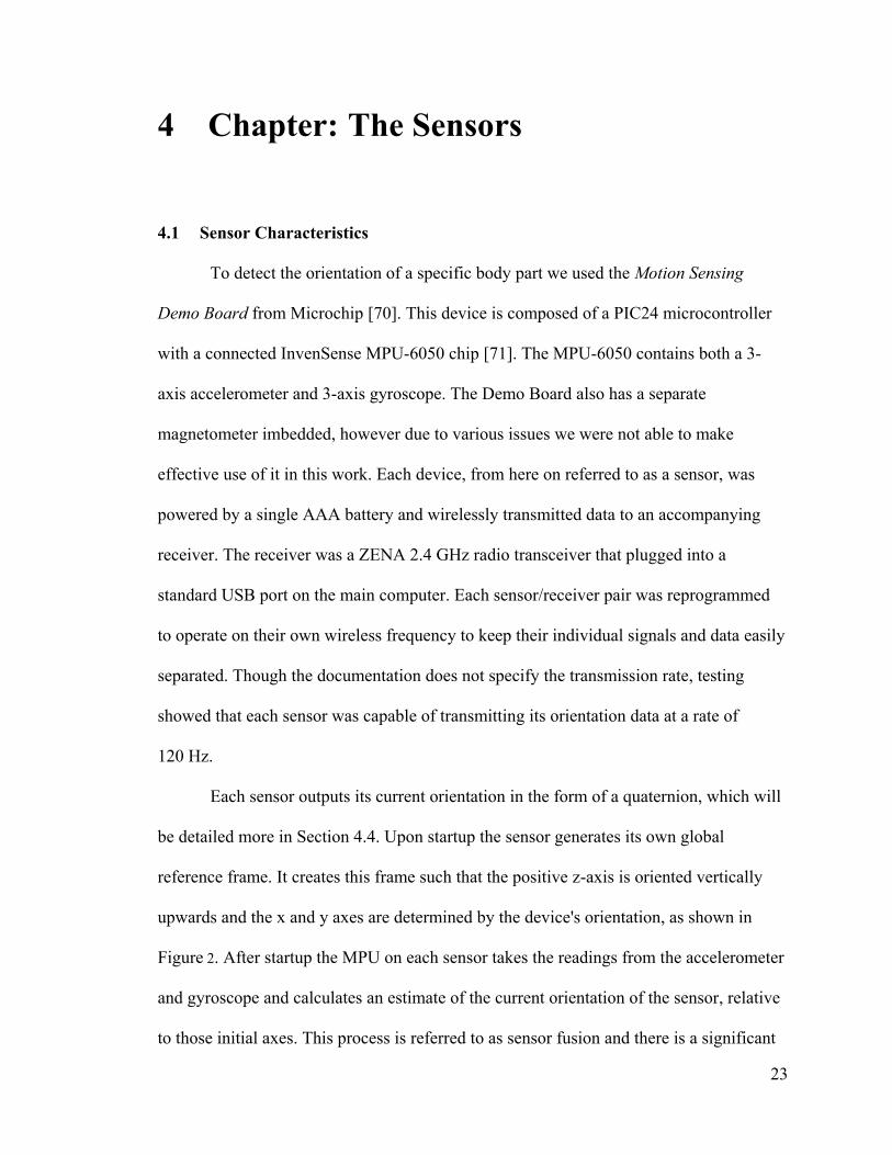
To detect the orientation of a specific body part we used the Motion Sensing
Demo Board from Microchip [70]. This device is composed of a PIC24 microcontroller
with a connected InvenSense MPU-6050 chip [71]. The MPU-6050 contains both a 3-
axis accelerometer and 3-axis gyroscope. The Demo Board also has a separate
magnetometer imbedded, however due to various issues we were not able to make
effective use of it in this work. Each device, from here on referred to as a sensor, was
powered by a single AAA battery and wirelessly transmitted data to an accompanying
receiver. The receiver was a ZENA 2.4 GHz radio transceiver that plugged into a
standard USB port on the main computer. Each sensor/receiver pair was reprogrammed
to operate on their own wireless frequency to keep their individual signals and data easily
separated. Though the documentation does not specify the transmission rate, testing
showed that each sensor was capable of transmitting its orientation data at a rate of
120 Hz.
Each sensor outputs its current orientation in the form of a quaternion, which will
be detailed more in Section 4.4. Upon startup the sensor generates its own global
reference frame. It creates this frame such that the positive z-axis is oriented vertically
upwards and the x and y axes are determined by the device's orientation, as shown in
Figure 2. After startup the MPU on each sensor takes the readings from the accelerometer
and gyroscope and calculates an estimate of the current orientation of the sensor, relative
to those initial axes. This process is referred to as sensor fusion and there is a significant
24
amount of literature written on the topic. The exact details of the fusion algorithm used
by InvenSense are not given in the documentation nor are they accessible through the
demo board's code. We will detail the basic fusion concept here and should the reader
wish to explore the topic further they can consult [53], [54] or [72] for more detailed
discussions.
Figure 2. The directions the sensor generates its global x and y axes.
4.2 Sensor Fusion
The sensor's onboard gyroscope can measure any rotations of the sensor and is
especially adept at quick rotations as previously discussed in Section 2.2. Since the
gyroscope has no absolute orientation capabilities the accelerometer's measurement of the
direction of gravity is used as a non-varying reference for the downward direction. Over
short time spans the gyroscope is used to determine any changes in orientation. Over
longer time periods the accelerometer's constant reference for the downward direction is
used to compensate for the gradual drift of the gyroscope. This allows the two different
sensor types to play off of each other's strengths and weaknesses to good effect. Kalman

25
filters or other similar filtering algorithms determine how each sensor contributes to the
overall orientation calculation [73].
Unfortunately, the accelerometer only provides a reference for the vertical/zenith
direction. Because of this, the gyroscope is able to freely drift about the vertical axis. This
results in the sensor's global x and y axes slowly rotating with respect to the actual global
frame. For this reason magnetometers are often used to anchor this rotation using the
Earth's magnetic field direction in the same manner as the accelerometer uses gravity.
Our sensors' fusion algorithm did not make use of a magnetometer and so we wanted to
obtain an estimate of approximately how much drift they experience.
4.3 Sensor Drift
A simple experiment was devised measure the drift. We compared the sensor's
reported orientation at various times when the sensor's actual orientation remained
unchanged in order to compute the drift about the vertical z-axis. In doing this we
assumed there was no significant drift about the other axes, which the resulting data
supported.
Figure 3 below shows the amount of drift since the sensor's startup under multiple
conditions. The stationary condition represents no motion of the sensor at all, with the
drift amount recorded every second. In the second condition, constant motion, the sensor
was in constant random motion except when it was returned to its starting orientation in
order to sample the drift. The drift in this case was sampled at ten second intervals to give
enough time between samples to move and rotate the sensor. In the final condition of

26
delayed motion the sensor was left in its starting position for the first 70 seconds and then
began random motion between drift samples.
Figure 3. Plot of the sensor's drift about the vertical axis over time under three different conditions.
A distinct drop off in drift rate is seen at the 13 second mark for the stationary and
delayed motion conditions. This drop off can be seen even more clearly in Figure 4,
which presents a magnified view of the first two minutes. Without allowing the sensors
this initial stationary time, the drift continues to accumulate seemingly indefinitely under
constant motion. The delayed motion condition shows that having the sensor in motion
continues to cause drifting, though the rate is significantly slower when this initial 13
second rest period is given. Though not shown on the plots, the condition of initial
motion followed by a stationary period and then more motion was also tested. The result
was a combination of the motion and delayed motion cases. The sensor drifted rapidly
until the motionless period was allowed, after which it drifted at a much slower rate. This
0
10
20
30
40
50
60
70
80
90
100
110
0 25 50 75 100 125 150 175 200 225 250 275 300 325
Dri
ft (
deg
rees
)
Time (seconds)
Stationary Constant Motion Delayed Motion

27
indicates that this 13 second rest period is extremely important to minimize the drift rate
of the sensors.
Figure 4. Magnified view of the first two minutes of sensor drift, highlighting the sudden change after
13 seconds when device is stationary.
These 13 motionless seconds matches the time it takes for the sensor to enter a
"low-power" state, which drops the data output rate to only 50Hz. Once the device
detects motion again it resumes the normal full data output at 120Hz. None of the
accompanying documentation discusses either of these issues, nor could any
accompanying code be found to clarify or modify these behaviours. However, it is likely
that this motionless time is needed, at least in part, for the fusion algorithm to properly
estimate noise and offset parameters for its orientation calculations. For all future
discussions in this thesis the sensors were given this required resting time on powering up
in order to minimize drift.
0
5
10
15
20
25
30
0 10 20 30 40 50 60 70 80 90 100 110 120 130
Dri
ft (
deg
rees
)
Time (seconds)
Stationary Constant Motion Delayed Motion

28
4.4 Quaternions
Each sensor outputs its orientation in quaternion form. Quaternions are a number
system originally devised by William Hamilton in 1843. A quaternion is comprised of a
scalar component, as well as a vector component located in complex space. This
representation can be seen in equations 1 and 2 below.
(1)
(2)
Here , and are the complex orthogonal basis vectors. Due to their complex nature
quaternion multiplication is a non-commutative operation. Table 1 shows the results from
the different basis multiplications. Equation 3 shows the full multiplication result for two
general quaternions, a and b. We will forgo rigorous proofs in this section, as the goal
here is to merely provide sufficient knowledge to permit an unfamiliar reader to be able
to understand later sections.
Table 1. Results of multiplication of the quaternion basis vectors
1 i j k
1 1 i j k
i i -1 k -j
j j -k -1 i
k k j i -1
29
(3)
The complex nature of quaternions means that we can define the complex conjugate,
denoted by the * superscript, of a quaternion q.
(4)
This allows us to also define the inverse, q-1
, of a quaternion q, such that q q-1
= 1.
(5)
In the event that q is a unit quaternion, having a magnitude of 1, the inverse will be equal
to the conjugate. All quaternions that represent a 3D rotation are represented by unit
quaternions. Quaternions are extremely efficient at representing rotational and orientation
information. A rotation of angle θ about a unit axis can be represented by the
quaternion shown in Equation 6.
(6)
To rotate the current rotational state q0 by the amount specified by q1, we multiply by q1
on the left side of the current state,
(7)
This quaternion q2 is equivalent to rotating by q0 and then rotating by q1. A series of
rotations can therefore simply be represented by a series of quaternion multiplications.

30
This is an extremely efficient method to compute and represent a series of rotations. It
must be remembered though that due to the non-commutivity of quaternions that the
order of these operations is very important.
A standard vector in three dimensions, , can be represented in quaternion form
by setting the real component equal to zero.
(8)
We can rotate this vector by any quaternion rotation q by multiplying the vector on both
sides.
(9)
The first step follows from Equation 5 and the fact qq* is equal to the magnitude of q.
The second step is the result of quaternion rotations having a magnitude of one.
Quaternions have many benefits over other rotational representations [74]. As
they do not require the calculation of many trigonometric functions they are very
computationally efficient. One of the biggest benefits to quaternions is that they do not
suffer from the issues of gimbal lock that methods like Euler Angles have. Euler Angles
also have degenerative points at the poles that are not unique. Despite these benefits,
quaternions do suffer from being more conceptually difficult and not as easy to visualize.

31
5 Chapter: Inertial Motion Tracking
5.1 Sensor Placement
In our system we wished to use the sensors to track the pose and motions of an
individual. In order to accomplish this we created specially designed cases to hold the
sensors using a 3D printer. Attaching Velcro straps to the cases allowed them to be easily
secured to the body. A case with a sensor inside can be seen in Figure 5. In total we
acquired ten sensors for use in our system. By securing a sensor to a body segment,
hereafter referred to as a "bone", the changes in orientation of the bone would be
equivalent to the changes in orientation of the attached sensor. The ten bones selected
were the left and right upper arms, forearms, thighs, and shins, as well as the torso and
pelvis.
Figure 5. Image of a sensor in its 3D printed case with the Velcro strap.
One sensor was assigned to each bone and each sensor was programmed to
operate on its own specific frequency channel. The positions of the sensors and the

32
corresponding frequency channels can be seen in Figure 6. Having a specific sensor
channel attached to a predetermined bone allowed the program to easily know where to
attribute the orientation information within the program. For example, the sensor
operating on frequency channel 13 must always be attached to the pelvis, as the system
will attribute the orientation data received on that channel to the pelvis bone within the
program.
Figure 6. Image showing the placement and operating channels of the sensors.
A robotic character model was created using the open-source software Blender
and is shown in Figure 7. The model consisted of all of the sensor-mapped bones, as well
as the hands and feet. A head was omitted so as to not obstruct camera view, as detailed
more in Section 5.9. The model was then imported into the Unity game engine [75] in
order to write scripts and animate the character based off of the sensor data. Each of the
bones was modeled as a separate object to allow greater control of their individual
positions and orientations than if they had all been part of the same object. Though the

33
hands and feet were also separate objects, for our purposes they were rigid and moved
and rotated in conjunction with their parent bone.
Figure 7. Character model created in Blender for the motion tracking game.
5.2 Bone Orientation Mapping
Upon startup, each sensor generates its own global reference frame. All of its
reported quaternion orientations represent rotations with respect to that initial reference
frame. Figure 8 below shows the initial startup frame generated by a sensor, its
orientation once it has been secured to the right upper arm, and the initial orientation of
the upper arm model in Unity's coordinate system. The quaternion reported by the sensor
in panel b) would be that it has undergone a 90 degree rotation about the y-axis. The
sensor's global frame differs from Unity's. Unity has the z-axis going into the screen,
whereas the sensor generates its z-axis upwards. This results in Unity having a left-
handed coordinate system as opposed to the sensor's right-handed system. If this

34
quaternion rotation is applied to the character's arm, not only will this cause the model's
arm to rotate away from its starting position, which currently matches the user's, it will
also not rotate in the way the sensor is indicating due to the different definitions of the
axes.
Figure 8. a) Orientation of the sensor on device startup with its generated global axis frame. b)
Sensor on the right upper arm with its generated global reference frame. c) Charcter's arm
orientation with Unity's axis frame.
In order to map the player's motions to the character, we had to resolve these two
issues. First, we needed to convert the quaternion from the sensor's global frame to the
Unity frame in order for the rotation directions to match correctly. Secondly, we had to
find a way to offset the quaternion value so that the orientation of the character's bones
matched those of the user at the start of the program.
5.3 Coordinate System Transfer
The two different coordinate frames are seen in Figure 8, under the condition that
at sensor startup we make the x-axes parallel. Under this condition Unity's z-axis goes
into the computer screen, corresponding to the sensor's y-axis. Similarly, Unity's vertical

35
y-axis corresponds to the sensor's z-axis. This provides the basic mapping for our system,
with our y and z values simply being swapped.
Due to the change in system handedness however, all of our rotations would
currently be going in the incorrect direction within the Unity program. Right-handed
systems rotate around an axis in a counter-clockwise direction, where left-handed
systems rotate in a clockwise manner. Referring back to Equation 6, we change the value
of θ to - θ in order to ensure proper rotation direction. Here we take advantage of the
even/odd nature of the sine and cosine functions. The negative can be pulled outside of
the sine function, while simply eliminating the negative in the cosine function. Therefore,
the final mapping from raw sensor quaternion q0 to the Unity remapped quaternion q0' is
given by
(10)
For easier readability we have omitted the i, j, k bases, since it is implicit based on
their position in the 4-vector. For the remainder of our discussions, when talking about a
raw quaternion from the sensor we will use q and when referring to the remapped version
we will use q'.
5.4 Initial Quaternion Offset
Now that we have solved the coordinate system discrepancy we need a way for
the orientation of the onscreen character's bone to properly match that of the player's. To
accomplish this, when starting the program we have the player stand in the matching
attention pose of the character, shown in Figure 7. At this point in time we know that the

36
player and character are in the exact same position. From Equation 7, we know that a
series of rotations in quaternion form can be represented by a sequence of multiplications.
If we define q0' to be a sensor's quaternion output at this attention pose and qt' to be any
other valid orientation at a later time t, then there exists another rotation, q1', that takes q0'
to qt'. More formally written, we have
(11)
This rotation, q1', is the rotation we want our bones to use for their orientation.
We are not interested in any rotations the sensor underwent to get to the starting attention
pose. Since the player and character are in the same pose at the start of the program, we
only want to rotate the bone the amount corresponding to the player's movements after
having started the program. On program startup we record the first quaternion output by
each sensor, q0'. At any later time t, we want our model's bone to therefore rotate by,
(12)
This equation was derived based on several of the properties presented in section 4.4. By
doing this we reset the starting orientation of each sensor to be its orientation relative to
when the program started, rather than when the sensor was turned on. An alternative way
of looking at this is that we are removing the rotations that occurred before starting the
program, q0', from the total rotation reported at a later time, qt'.
One more additional offset is required for each bone. When importing the
character from the 3D modeling program to the game engine, the bones obtain a
rotational offset. Even though the character is in the proper pose each bone is not in its

37
zero rotation orientation. Therefore, when assigning a bone the total rotation given by
Equation 12, the result is incorrect by this imported offset amount. This rotation is a
simple 90 degree rotation around the x-axis and is the same for every bone. We want this
rotation included in our calculation so that the bone starts in the proper attention pose
orientation before rotating to match the player. From Equation 6, this imported rotation,
qI, is given by
So, the final quaternion that represents the total rotation we wish our bone to have is
therefore given by
(13)
This method of obtaining the matching orientation has inherent benefits and
weaknesses. When attaching the sensors to the player's body, extreme care is not required
as to the sensor's exact orientation with respect to the body part. These potential
orientation differences when securing the sensor are eliminated from the calculation since
all rotations are relative to the initial starting orientation. The main factor determining
tracking accuracy is how closely the user matches the pose of the character at startup.
While there will certainly be some small discrepancies between the user and the
character, the differences are likely very small with such a basic and natural pose. It is
important however, that once running the sensors do not slip or move relative to their
attached bone. Slipping of a sensor will cause a discrepancy in the orientation of the
character's bone relative to that of the player. While the actual manifestation may be
different, all marker-based systems will suffer accuracy issues from sensor slipping.
38
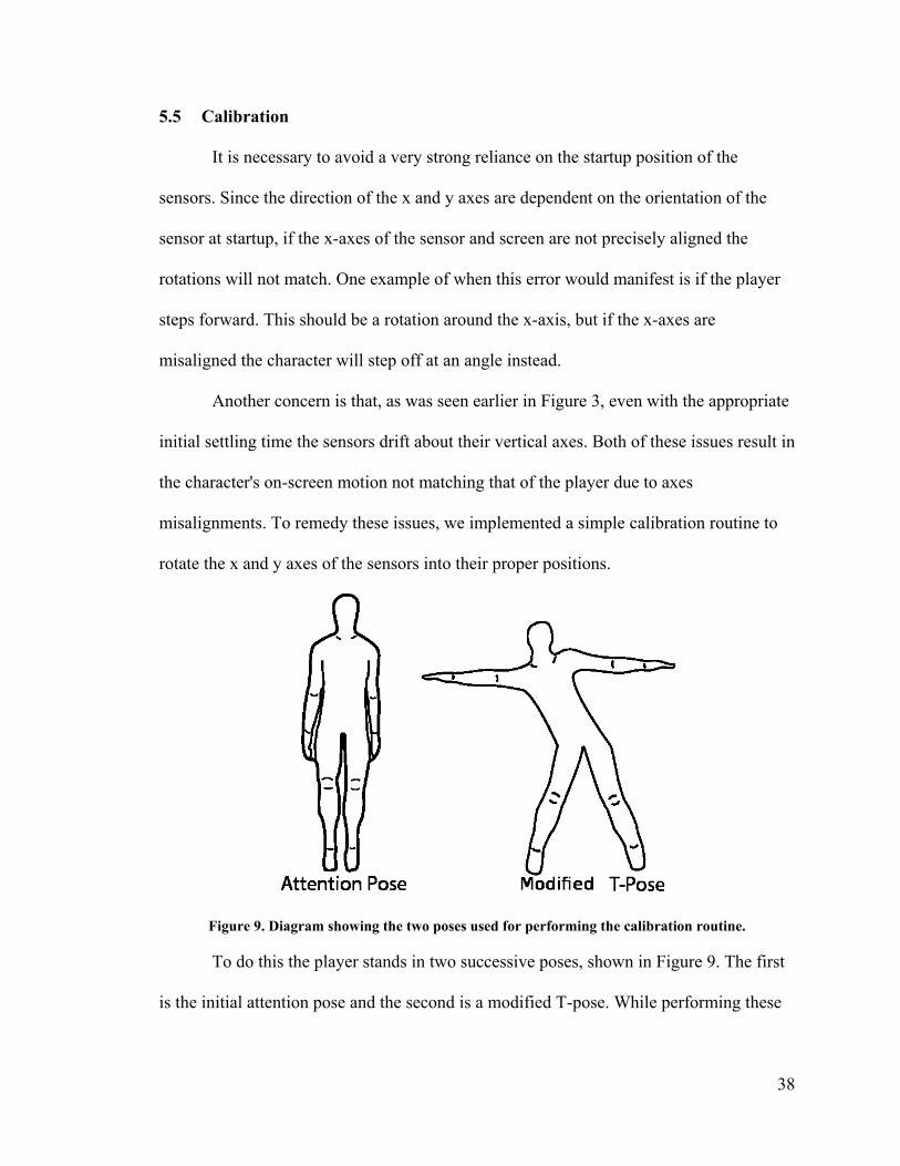
5.5 Calibration
It is necessary to avoid a very strong reliance on the startup position of the
sensors. Since the direction of the x and y axes are dependent on the orientation of the
sensor at startup, if the x-axes of the sensor and screen are not precisely aligned the
rotations will not match. One example of when this error would manifest is if the player
steps forward. This should be a rotation around the x-axis, but if the x-axes are
misaligned the character will step off at an angle instead.
Another concern is that, as was seen earlier in Figure 3, even with the appropriate
initial settling time the sensors drift about their vertical axes. Both of these issues result in
the character's on-screen motion not matching that of the player due to axes
misalignments. To remedy these issues, we implemented a simple calibration routine to
rotate the x and y axes of the sensors into their proper positions.
Figure 9. Diagram showing the two poses used for performing the calibration routine.
To do this the player stands in two successive poses, shown in Figure 9. The first
is the initial attention pose and the second is a modified T-pose. While performing these
39
poses the player faces square to the play screen. The player has several seconds to
transition between each pose when prompted by the program.
The modified T-pose was designed to have all of the bones and sensors undergo a
rotation when transitioning from the attention pose, which allows us to individually
calibrate each sensor. Between these two poses the player stays confined within a plane
which is parallel to that of the play screen. This means that there is no movement by any
of the bones towards or away from the screen. Therefore, this allows us to have the
rotational axis between these two poses to point directly towards the screen for all the
bones.
We will denote the sensor's reading in the attention pose by qA' and the reading in
the modified T-pose by qT'. We start with a simple downwards unit vector (in quaternion
form) in the Unity frame, given by
We want to determine what axis the sensor rotated around between the attention and
modified T-poses. If we use Equation 9 and the same logic that we used to get to
Equation 12, we can write
(14)
Here, v1 is the new vector resulting from rotating the initial v0 through the same rotation
the sensor underwent from the attention pose to the modified T-pose.
With the axis of rotation for all of the bones being along the player to screen
direction, this corresponds to the z-axis of Unity's frame. This ideally would also
correspond to the y-axis of the sensor's frame, though due to the aforementioned issues

40
this may not be exactly correct. Instead, the sensor will report this as a rotation around a
combination of both the x and y axes rather than purely the y-axis. This concept can be
seen in Figure 10 below.
Figure 10. Diagram showing the rotation axis between the attention pose and T-pose in both Unity's
and sensor's reference frames.
We need to determine the rotation angle, , between the ideal and current sensor
reference frames. We start by taking the cross product between our v1 and v0 vectors.
Since we are using the remapped frame quaternions, this gives us a vector located
entirely in the xz-plane. Note that here we have switched our vectors into the classic three
term form and also since we are in a left-handed system the cross product is taken
appropriately.
(15)
From this we are able to determine our angle of drift using trigonometry.

41
(16)
This is true for the right side of the body and the torso. The left side of the body is
rotating in the reverse direction, thus giving a cross product vector pointing in the
opposite direction. We therefore must add an additional π to the drift angle for the bones
on the left side.
Now that we have calculated the amount of drift for each sensor, we can use this
to adjust our remapping to properly align the different reference frames. Previously we
determined the mapping between the raw sensor quaternions and the Unity quaternions in
Equation 10. Post-calibration, we wish to rotate this mapping around the vertical axis so
the sensor's reported y-axis properly aligns with Unity's z-axis. Using the standard
rotational equations we find that our new calibrated mapping, qcal
, is given by,
(17)
where q is the raw sensor output.
This calibration procedure can be repeated at a later time to determine an updated
value for , should the sensors drift enough during play that it becomes an issue. This
calibration method does not align the frames perfectly since it is dependent on the player
rotating around the axis perpendicular to the screen. However, informal testing showed
that any differences from the ideal were not perceptible to users. It also has the benefit of
being very simple and quick to perform, requiring less than fifteen seconds on the part of
the user.

42
It is worth noting that the pelvis and attached sensor do not undergo any
significant rotation between the two calibration poses. Unfortunately no simple pose
results in a significant rotation of the pelvis area, and so this rotation was left out of the
calibration. Since all the sensors drift in a reasonably similar manner, the drift angle
determined for the torso can be used as an approximation for the pelvis. While not ideal,
the pelvis rarely undergoes rotation about either of the horizontal axes. Since rotations
about the vertical axis are not affected by drift issues, any drift in the pelvis readings
would be significantly less noticeable than it would be for any of the other bones.
5.6 Orientation Overview
With the actual details of the mapping and tracking mathematics explained, a
more detailed sequence of the steps the system undergoes is beneficial to better
understand both how the system works, as well as the experience of the player. Once the
player has secured all of the sensors to the appropriate bones, as shown in Figure 6, they
are ready to start the program. On start-up the player is prompted to stand in the attention
pose, as seen in Figure 9. At the end of an on-screen countdown (we used 4 second
durations) the current quaternion of each sensor is sampled. The user is then prompted to
move to and hold the modified T-pose. At the end of the countdown the quaternion of
each sensor is again sampled. These two quaternions are used to obtain the offset angle
for each bone/sensor pair, which in turn is used to obtain the remapping between the
sensor and program reference frames using Equation 17.
The user is then instructed to return to the attention pose, which matches that of
the player's robotic character. At the end of the countdown each sensor is again sampled.
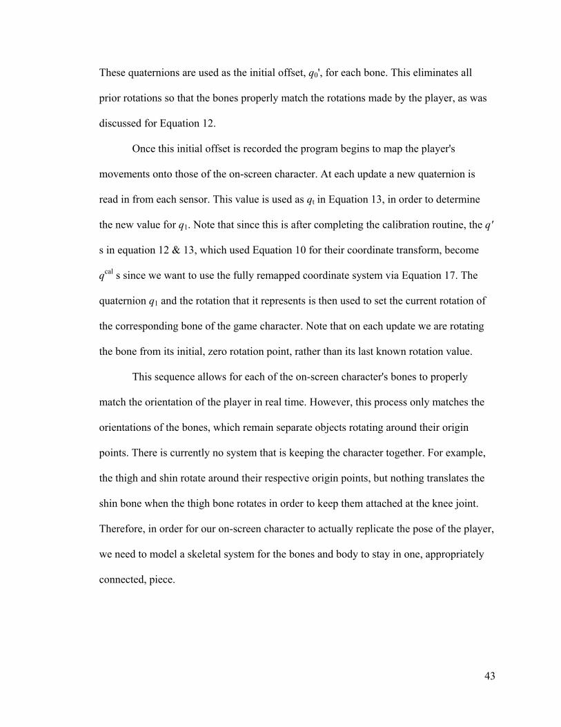
43
These quaternions are used as the initial offset, q0', for each bone. This eliminates all
prior rotations so that the bones properly match the rotations made by the player, as was
discussed for Equation 12.
Once this initial offset is recorded the program begins to map the player's
movements onto those of the on-screen character. At each update a new quaternion is
read in from each sensor. This value is used as qt in Equation 13, in order to determine
the new value for q1. Note that since this is after completing the calibration routine, the q'
s in equation 12 & 13, which used Equation 10 for their coordinate transform, become
qcal
s since we want to use the fully remapped coordinate system via Equation 17. The
quaternion q1 and the rotation that it represents is then used to set the current rotation of
the corresponding bone of the game character. Note that on each update we are rotating
the bone from its initial, zero rotation point, rather than its last known rotation value.
This sequence allows for each of the on-screen character's bones to properly
match the orientation of the player in real time. However, this process only matches the
orientations of the bones, which remain separate objects rotating around their origin
points. There is currently no system that is keeping the character together. For example,
the thigh and shin rotate around their respective origin points, but nothing translates the
shin bone when the thigh bone rotates in order to keep them attached at the knee joint.
Therefore, in order for our on-screen character to actually replicate the pose of the player,
we need to model a skeletal system for the bones and body to stay in one, appropriately
connected, piece.

44
5.7 Skeletal Model
Initially we allowed Unity to take care of positioning all the bones on its own. It
has its own system built in that can allow it to keep track of the bones and make sure they
stay attached. However, by allowing Unity to do this for us, we were losing control of
several factors, including the order that the bones were updated. This led to poorer
performance and a lower quality tracking result. Therefore, we elected to create our own
skeletal model to handle the positioning of all the bones.
5.7.1 Bone Base and Tip Positions
The position of a bone's base, pb, refers to the point in space which it naturally
rotates around. For example, the forearm's base is the elbow, the upper arm's base is the
shoulder, and so on. The bone's tip, pt, is the position where the next bone attaches. For
the upper arm this would be the elbow and for the thigh this would be the knee. We will
define a bone's length vector, , to refer to the vector which points from the bone's base
position to the tip of the bone at the start of the program. At any later time, with the
bone's orientation q1cal
, we can calculate the tip position by,
(18)
This is the q1cal
, given by Equation 12, and not 13, as the imported offset is already
included in the calculation through the recording of the length vector at its initial
position. Given that all the bones are connected, the position of the tip of one bone will
be the base position of the next bone. Using this we can sequentially calculate the
positions of the bones from one to the next like a chain, updating all of their positions
appropriately.

45
In addition to better control over how and when the character gets updated, our
skeletal model gives us an easy way to allow the character to "walk" in the virtual world.
This is not something that other works like [23] have done. They instead have their
virtual character suspended in space, with the pelvis being an immobile point from which
all bone positions are calculated. For them, walking entails sliding the feet on the ground,
and crouching brings the feet up to the body, rather than lowering the body down to the
feet.
5.7.2 Skeletal Walking Design
We know the lengths and orientations of both the thigh and shin bones of each
leg. The tip of the shin bone corresponds to the position of the foot. Therefore, the shin
bone tip with the lower vertical position can be treated as the foot that is "planted" on the
ground. When a foot is planted it isn't moving and all rotations of the rest of the body
take place around this planted foot.
In the program we set a condition that checks the height of the two feet.
Whichever foot (i.e. shin bone tip) has the lower position remains fixed in the game
space. Equation 18 above was created for setting the proceeding bone's base position,
based on the current bone's tip position. Since we want our planted foot's tip to remain
stationary we wish to do the opposite and use this bone's base position as the next bone's
tip position. Essentially, we want to calculate the chain from the foot back up to the
pelvis, rather than from the pelvis down to the foot. This is simply reversing the base and
tip positions. For the planted leg we can write that
(19)

46
Once the pelvis' position has been calculated from the planted foot the rest of the
remaining bones may be calculated in the original base-to-tip manner of Equation 18.
Calculating the lower position of the two feet works well in theory. In practice
there is noise on the sensor outputs. When standing on both feet, the selection of which
foot was considered planted often quickly jumped back and forth, causing perceptible
jitter in the on-screen character. To remedy this, we added a distance, ε, that the non-
planted foot must be below the planted foot in order for the program to switch which one
was considered planted. After some trial and error we settled on a value of ε = 0.0005
Unity units.
This correction would cause the player to slowly but steadily move downwards,
as each step would cause them to drop by another 0.0005 units on the vertical axis. To
prevent this, on each frame update, the planted foot and hence rest of the body are moved
half of the distance back to the ground plane height of y=0. This allows for a smooth
transition back to the ground plane that is too small for users to notice but prevents the
gradual sinking of the player.
This skeletal system allows the user to perform a wide range of actions such as
walking, crouching and leaning. However, the system does have its limitations in its
current form. Since we do not have any sensors on the feet we cannot detect ankle angles
and are essentially ignoring the presence of the player's foot, which is obviously not an
accurate representation. For any motions where the feet both stay close to the ground the
system will sometimes struggle to determine the correct planted foot due to slight
inaccuracies. We also have one foot always planted to the ground, eliminating the ability
of the system to display jumps. Nevertheless, the system works well for the vast majority
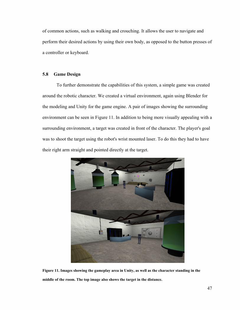
47
of common actions, such as walking and crouching. It allows the user to navigate and
perform their desired actions by using their own body, as opposed to the button presses of
a controller or keyboard.
5.8 Game Design
To further demonstrate the capabilities of this system, a simple game was created
around the robotic character. We created a virtual environment, again using Blender for
the modeling and Unity for the game engine. A pair of images showing the surrounding
environment can be seen in Figure 11. In addition to being more visually appealing with a
surrounding environment, a target was created in front of the character. The player's goal
was to shoot the target using the robot's wrist mounted laser. To do this they had to have
their right arm straight and pointed directly at the target.
Figure 11. Images showing the gameplay area in Unity, as well as the character standing in the
middle of the room. The top image also shows the target in the distance.

48
To determine if this condition was met, every bone was given a directional vector
that pointed along the bone's length. This is very similar to the length vector, , used in
Equation 18. However, a new vector was needed for this purpose since some bones, like
the upper arm, have length vectors that do not point exactly along their bone length. Both
the forearm and upper arm start with initial direction vectors of
This vector follows from the player starting in the attention pose, with their arms at their
sides pointing straight down. At a later time the pointing vector for the forearm, vf, and
upper arm, vu, can be determined by
(20)
(21)
We determine if the arm is straight, with no significant bend at the elbow, by
taking the dot product between vf1 and vu1. If the result of that dot product is above a
certain threshold (we used a threshold of 0.95) then we can classify the arm as straight.
We perform a very similar operation to determine if the arm is pointed to the
target. To do this we calculate the vector from the upper arm base position (the shoulder),
pu, to the target's center, pT. We normalize this vector so that the target's distance from
the character is irrelevant, as all we are interested in is the direction.
(22)
We then take the dot product between this target vector and the pointing vector of the
upper arm, though using the forearm would be equally valid. If the result is above a

49
certain threshold (we used a threshold of 0.975) the arm was considered to be aiming at
the target.
When both of these conditions are met, we know that the player has a straight arm
and that it is pointed at the target. We then trigger the "hit" condition, which fires the
player's laser, has the target explode into several pieces, and plays an accompanying
audio clip. A few seconds after the target has been destroyed a new one is generated in a
random position in front of the player for them to shoot. After three successful hits the
targets begin to move to increase the challenge level.
5.9 Oculus Rift Integration
The initial gameplay used a 3rd person over-the-shoulder perspective. However, it
was found that this was not the most effective use of the system. Looking at the character
on the screen, the player would frequently have difficulty aiming at the target due to the
1:1 motion mapping. The player was not aiming at the target on the screen, but instead
was trying to judge where the target would be from the robot's perspective. Though not as
significant, there was also an issue with a lack of depth information. The player did not
really know if the target was a hundred meters away from them or only a few meters
away. These issues unintentionally increased the difficulty of hitting the target, in a way
that was somewhat frustrating for the player.
To help resolve both of these issues an Oculus Rift (Development Kit 1) [19] was
incorporated into the system. The Rift is a head mounted display that features both head
tracking and full 3D depth perception by having a separate image presented to each eye.
This device was integrated into the game project and the virtual camera was moved atop

50
the character model to generate a first person perspective. This is why the final character
model in Figure 7 has no head. The geometry of the modeled head interfered with the
camera view through clipping and obstruction issues once the camera was moved to this
first-person perspective. The virtual camera was also tracked to the movements of the
player's torso. This allowed any motions the player made to cause the camera view move
and shift the in-game perspective appropriately.
While no quantitative testing was performed to compare the two game
perspectives, it was apparent that using the first person view made hitting the target
appreciably easier and less frustrating. Players were able to point their arm at the target
much quicker and with much less adjusting when trying to find the "trigger spot". They
also appeared more relaxed, moving more naturally and with their whole body rather than
standing rigid while concentrating on only their shooting arm.
An additional effect of incorporating the Rift was a heightened level of immersion
within the game. Being immersed in the fully 3D virtual world with accurate head and
full body (less the hands and feet) tracking added significantly to both the game itself, as
well as to the perceived novelty of the body tracking. The two figures below show a pair
of joint image of a user playing the game with the Rift, adjacent to the in-game view.
51
Figure 12. Image showing a user playing the game with the Oculus Rift.
Figure 13. Image of a user playing the game and shooting the target.
5.10 Limitations and Issues
There were some downsides to incorporating the Rift into the game. The entire
virtual scene had to be scaled down in order to prevent the player from feeling like they
were massive in size. The much closer view of the character also made the noise and
jittering in the sensor outputs more apparent. Smoothing the quaternion values between
their current and previous values reduced the jittering, though it did not eliminate it
entirely. The development version of the Rift that we used is a wired device, which
limited the player's ability to move around. However, with their real-world vision
obscured by the Rift, substantial walking around would not be recommended anyway.

52
Some issues were encountered with the update rate of sensor information. Small
stutters in the game of about half a second in length occurred when the system was
waiting to get a reading from a sensor. This would cause the character to momentarily
freeze, and even more jarringly caused pauses in the display update for the Rift. It is not
entirely clear why this occurred, as the update rate of the sensors should be sufficient to
avoid this. It may be that the library used to access the USB ports [76] within Unity was
not well optimized to handle that many USB connections at a time, which could cause
these hiccups.
To help with this, the portion of the code that handled reading in the sensor data
was moved to a separate CPU thread. This separated the motion tracking from the
display, resolving the display stuttering problem. However, it did not significantly
improve the pauses in the updating of the skeletal model. Waiting for one of the sensor's
data prevented the others from updating until the delayed one finished. The cause of this
problem is currently not entirely clear. It is possible that a single sensor is operating
poorly and causing these delays. This is an issue that requires further examination in the
future.
We will discuss this issue, along with a much more in-depth and broader
discussion on the sensors and motion tracking setup in Chapter 7. However, in this
chapter we have seen that our wireless inertial sensor network holds strong potential for
motion tracking applications. While we did not quantitatively test the system due to time
constraints, it performed well in the active game we developed and was well suited for
combining with a virtual reality environment. While the drift of the sensors was an issue,
this was mitigated by the development of a calibration routine. Meanwhile, the

53
hierarchical skeletal model allowed for controller-free navigation of the virtual world.
While there are still areas which could be improved, the current system is a strong
functional foundation upon which to build in the future.
54
6 Chapter: Gesture Recognition
Our goal was to have a unified motion tracking and gesture recognition system.
Therefore, we use the same sensors to perform gesture recognition on the user's actions as
those used for the motion tracking. In this way the same system can be used for both
purposes simultaneously. To do this we require an algorithm for performing the gesture
recognition. One of the most commonly used methods is the Hidden Markov Model
(HMM).
6.1 Hidden Markov Model Theory
An HMM represents a sequence of states as a stochastic process that proceeds
through a series of time steps. Each time step in the sequence transitions from one state to
the next, with these changes governed by the transition probabilities. This process obeys
the Markov property, in that the next state is dependent only on the current state and not
on those which came before it. For each state the observed output is a symbol from a
predefined alphabet. The symbol that is output from a particular state is governed by the
emission probabilities for that state. An HMM may be parameterized as ,
where:
A total of N possible states, given by S = {S1, S2, S3, ..., SN}.
A total of M possible output symbols C = {C1, C2, C3, ..., CM}.
The NxN transition matrix A, where the matrix element aij is the probability of the
state Si transitioning to state Sj.
55
The NxM emission matrix B, where the matrix element bij is the probability of the
state Si outputting symbol Cj.
Finally, π is the initial state distribution vector, π = {π1, π2, ..., πN}
A specific HMM is determined by its transition probability matrix A and emission
matrix B. These matrices can be estimated through a training process by observing
example state sequences. The training and recognition algorithms make use of the Baum-
Welch and Viterbi algorithms, which can be found in more detail in [77].
Each gesture to be recognized has its own individual model. Once each of the
various models have been trained they may be used for gesture recognition. A given input
sequence is tested against each of the gesture models. Each model determines the
likelihood that the test sequence was generated as the result of its transition and emission
probabilities. Based on these outputs the test sequence is recognized as the model (and
thus the associated gesture) that produced the highest likelihood.
6.2 State Divisions
In order to perform recognition on our sensor data we first need to classify it into
states. We would like for these to be roughly evenly distributed over our vector space.
Our sensors report their raw quaternion value in the form q = (qw, qx,qy, qz). However,
these four values are not independent, since . We therefore need to
reparameterize the quaternion such that we have three independent variables. An easy
way to accomplish this is to convert from quaternions to Euler Angles. While the Euler
Angles have their weaknesses, as mentioned in Section 4.4 , we are performing the

56
continuous orientation updates completely within quaternion form and only recasting the
final value into Euler Angles. In this way we avoid many of the associated issues, such as
gimbal lock.
We also take note that the negative of a quaternion represents the same rotation as
its positive. That is to say,
Therefore, whenever qw is negative we can multiply the whole quaternion by -1 to ensure
that we do not have equivalent rotations being represented by two different states.
Though there are different parameterizations possible for the Euler Angles [78], we
elected to use
(23)
where
We are now in a position where we may find a way to uniquely classify the
current orientation value into a specific state. We divide each of our three (α, β and )
parameters' ranges of possible values into L sectors per π radians and give each sector an
individual state number from 0 to L-1. The parameter's state number is then determined

57
by which sector the parameter's actual value falls within. This concept is shown in Figure
14 for α. This will give rise to a total number of states given by
(24)
We can uniquely assign an overall state based on our three parameters' individual state
values by the equation
(25)
We have added the +1 at the end simply because we do not want a possible final state of
value zero.
Figure 14. Showing the possible αstate values in blue for the different angles of α and values of L.
Initial testing showed issues around the upper and lower extremes of the β values.
Due to the way all of the sectors converge at the poles for the α state, very small motions
can lead to multiple state changes. Even when trying to hold a steady pose there can be
significant flickering between many states when near these points. To remedy this, we
restricted the value of the α state for extreme values of the β state. This means that when
β is in its smallest state, βstate=0, or in its largest state, βstate=L-1, we removed the
dependence on αstate in the overall final state by setting αstate to a specific value. For

58
example, if we look at the case of L=3, the potential values of the βstate range from 0-2
and for αstate from 0-5. If βstate equals 0 or 2 we automatically set αstate to be 0 (any other
value in the range would work equally well) regardless of its true value. We therefore
eliminate its influence on the calculated overall state of Equation 25 and resolve the
converging issue at the pole.
While this adjustment does mean we have lost the ability to distinguish between
certain orientations within these regions, the affected area shrinks with increasing L. It
also eliminates the issues associated with the singularities at the two poles where the
values are ill-defined. Although we will keep Equation 25 to determine the final state
value, our actual total number of states has dropped to
(26)
Table 2 below shows the total number of possible states for a given value of L, as well as
the angle spanned by a single state.
Table 2. Total number of states for a given value of sectors (L) per π radians, and angle of rotation
spanned by a sector.
Value of L 3 4 5 6 7 8
Total States 48 144 320 600 1008 1568
Angle (Deg) 60 45 36 30 25.7 22.5
We elected to register and perform the recognition using only a single repetition
of a state rather than the full state sequence. The sensors output their orientation at
approximately 120Hz, so this means that the same state is repeated tens of times in a row
for even fast motions. These long sequences of repeat states slows down recognition time
significantly. To prevent this, we reduce an observed state sequence of [1,1,1,3,3,4,4,4,4]
to simply [1,3,4]. Removing these repeats also allows us to make the recognition

59
independent of time, meaning that so long as the same motion is made, it can be
recognized regardless of the speed with which it was performed.
The recognition algorithm and training programs themselves were written in C++
with Visual Studio 2010 as the integrated development environment. The program would
read in the sensor's current orientation in quaternion form and then convert it to the Euler
Angle form. It would then automatically convert this into a final orientation state value
through the process just described. If this new state was different from the previous state,
the new state would be added to the state sequence. Since each sector spans a range,
multiple quaternions can be mapped to the same final state.
6.3 The Gestures
We are currently able to track the full body motions of an individual using
multiple sensors. However, we elect to use only a single sensor for our gesture
recognition. The reasoning for this is that we wish to validate the accuracy of our
technique using a single sensor as a baseline before moving on to a multi-sensor
recognition setup. To do this, we used the sensor attached to the right forearm. We
wished to select gestures that made sense within the context of our robot-based action
game. In total six gestures were selected: Jab, Jets, Uppercut, Asgard, Throw and Block.
The motions associated with each gesture are shown in Figure 15. Some were purposely
chosen so that the gestures started at the same initial position. This was to verify that the
system could distinguish between gestures sharing common elements.

60
Figure 15. Diagrams depicting the motion for each of the six gestures that were used.
6.4 Methods
A total of 10 individuals contributed to the training of the system. They each
performed every gesture a total of 50 times, leading to a total of 500 training samples per
gesture and 3000 gesture samples in total. Two training sequences for the uppercut
gesture were not useable and so for that gesture there were only 498 training samples and
hence 2998 total gesture samples. However, this is not a significant enough difference in
the number of training samples to affect the uppercut gesture results.
Before starting each gesture training set the sensor was restarted to verify that its
frame aligned properly with the Unity frame. It was also given the required 13 seconds to
stabilize the drift. The sensor was then placed inside the case on the participant's arm.
This process was done between every set of gesture recordings. The reason for restarting
the sensor between every training set was to ensure that gradual drift was not throwing
off the readings of the later gestures compared to those recorded first.
An experimenter demonstrated in-person the correct way to perform each gesture
prior to the participant performing each gesture set. During the performance of the
training gestures an experimenter would start and stop the recording of data for each
individual gesture in the set. The participant would hold the starting pose of the gesture
61
and the experimenter would begin recording the gesture data. The experimenter would
then instruct the participant to perform the gesture. The participant would briefly hold the
ending pose of the gesture as well to allow the experimenter to stop the data recording.
Since the recognition is time independent these initial and final pauses are not imparted
onto the gesture's training data. Participants were allowed to perform the gesture naturally
and were only stopped and re-instructed in the proper way to perform the gesture if they
were seen to have noticeably drifted from the intended design. This was a subjective
judgment by the experimenter, who was common to all participants. This allowed for
more realistic variation in a user's performance of a gesture, rather than forcing them all
into a very specific motion.
None of the remapping or initial offset calculations performed previously in the
motion tracking chapter were performed on this data. These operations are simply
coordinate transformations and offsets of the raw quaternion values and so they should
not affect accuracy results. This is discussed more in Section 7.8.
6.5 HMM Testing
Using this training data we were able to test the system's ability to recognize
gestures using our Hidden Markov algorithm. Two situations were tested. The first case
is the user included (UI) condition, in which the individual who performed the gesture to
be recognized is included in the training set. To do this we used a test 10, train 40
method. Of the 50 samples given 10 were extracted at random to test with while the
remaining 40 were used as training for the gesture's HMM, along with all the data from
the other users. This process was repeated 250 times, 25 times per individual, to get an
62
averaged accuracy using different subsets of 10 sequences for testing and across different
users. For this condition all of the user's data samples that were not being used as test
samples were used for training.
The second condition is the user excluded (UE) case, where the testing participant
is completely excluded from the training. In this case none of the data from the
participant being tested was used in any of the training samples for any of the gestures.
All 50 of their gestures were tested against the training data from all other participants.
This is the most difficult recognition condition but also the one that resembles real-world
situations, since it represents the ability to simply pick up and use the system, without
requiring a training period before use.
6.6 HMM Results
Figure 16 shows the graph of the results from our HMM tests for the UI condition
and Figure 17 shows the results for the UE condition. The recognition accuracy reported
is the number of times the gesture was correctly identified divided by the total number of
gesture sequences tested. We treated equal recognition rates, that is, when the maximum
likelihood was shared across two or more gesture models, as a non-recognition since the
system could not uniquely determine the correct gesture. It is also possible for the system
to obtain a likelihood of 0 for all gesture models, which is also counted as a non-
recognition.

63
Figure 16. Recognition accuracies for the different gestures using the HMM with a varying number
of sectors, under the user included condition.
Figure 17. Recognition accuracies for the different gestures using the HMM with a varying number
of sectors, under the user excluded condition.
0
10
20
30
40
50
60
70
80
90
100
3 4 5 6 7 8
Re
cogn
itio
n A
ccu
racy
(%
)
Sectors per π radians
Jab
Uppercut
Jets
Asgard
Throw
Block
0
10
20
30
40
50
60
70
80
90
100
3 4 5 6 7 8
Re
cogn
itio
n A
ccu
racy
(%
)
Sectors per π radians
Jab
Uppercut
Jets
Asgard
Throw
Block

64
From these plots we can see that recognition rates vary significantly between the
different gestures. Most of the accuracies rapidly decrease as the number of sectors
increases. Several gestures demonstrate a parabolic-like trend, with an initial accuracy
increase with more sectors before quickly dropping again. This is likely caused by the
initial increase in the number of sectors increasing the system's ability to differentiate
between different motions due to the finer state divisions. Beyond a certain point the
small variations between users will result in completely different state sequences when
the state divisions are extremely fine. Not all of the gestures demonstrate this property
however. Instead, they just decrease in accuracy as the number of sectors increases.
As would be expected there is a significant difference between the UI and UE
conditions. Figure 18 shows the recognition accuracy averaged across all gestures for
both conditions at each sector value (the number of sectors used). We can see that for all
sector values the UI accuracy is higher than the UE. Both trends also clearly show the
parabolic-like shape previously discussed. For the excluded case the maximum accuracy
occurs at four sectors, whereas for the included case it occurs at five. The confusion
matrices are shown in Table 3 and Table 4 for these two conditions. The full list of
confusion matrices is shown in Appendix A.1 and A.2. In these tables the vertical column
of gestures are the gestures that were actually performed, whereas the horizontal gestures
are what the system recognized it as. The unrecognized column is for the cases where all
models returned 0 or when the maximum likelihood value was shared by two or more
gestures.

65
Figure 18. Accuracy at each sector value averaged across all six gestures with the HMM.
Table 3. Confusion matrix for the user excluded HMM case with four sectors per π radians.
Performed Recognized As (%)
Jab Uppercut Jets Asgard Throw Block Unrecognized
Jab 48.2 5.4 3.4 0.0 1.4 0.0 41.6
Uppercut 13.8 50.0 2.8 0.0 4.2 5.2 24.0
Jets 10.2 0.2 74.6 0.8 1.8 0.8 11.6
Asgard 8.6 0.0 5.6 68.4 4.0 2.4 11.0
Throw 9.0 1.2 8.0 0.0 43.0 12.8 26.0
Block 1.4 0.0 1.6 1.6 0.2 78.8 16.4
0
10
20
30
40
50
60
70
80
90
100
3 4 5 6 7 8
Re
cogn
itio
n A
ccu
racy
(%
)
Sectors per π radians
Excluded
Included
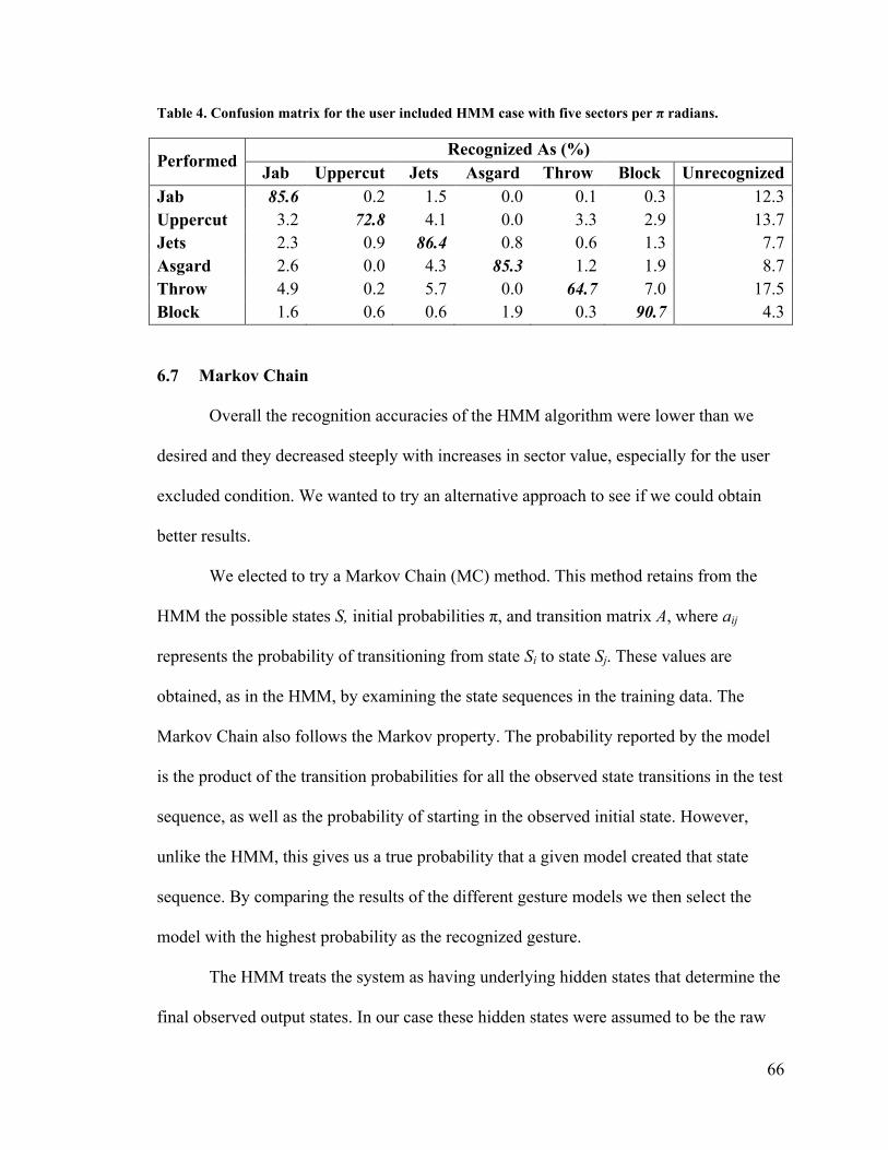
66
Table 4. Confusion matrix for the user included HMM case with five sectors per π radians.
Performed Recognized As (%)
Jab Uppercut Jets Asgard Throw Block Unrecognized
Jab 85.6 0.2 1.5 0.0 0.1 0.3 12.3
Uppercut 3.2 72.8 4.1 0.0 3.3 2.9 13.7
Jets 2.3 0.9 86.4 0.8 0.6 1.3 7.7
Asgard 2.6 0.0 4.3 85.3 1.2 1.9 8.7
Throw 4.9 0.2 5.7 0.0 64.7 7.0 17.5
Block 1.6 0.6 0.6 1.9 0.3 90.7 4.3
6.7 Markov Chain
Overall the recognition accuracies of the HMM algorithm were lower than we
desired and they decreased steeply with increases in sector value, especially for the user
excluded condition. We wanted to try an alternative approach to see if we could obtain
better results.
We elected to try a Markov Chain (MC) method. This method retains from the
HMM the possible states S, initial probabilities π, and transition matrix A, where aij
represents the probability of transitioning from state Si to state Sj. These values are
obtained, as in the HMM, by examining the state sequences in the training data. The
Markov Chain also follows the Markov property. The probability reported by the model
is the product of the transition probabilities for all the observed state transitions in the test
sequence, as well as the probability of starting in the observed initial state. However,
unlike the HMM, this gives us a true probability that a given model created that state
sequence. By comparing the results of the different gesture models we then select the
model with the highest probability as the recognized gesture.
The HMM treats the system as having underlying hidden states that determine the
final observed output states. In our case these hidden states were assumed to be the raw

67
values of the accelerometer and gyroscope. They are combined to give us our final
observed state, a quaternion which we then convert into a orientation state, but we cannot
observe these raw signals directly, hence they are "hidden" from us. The Markov Chain
forgoes these hidden states and instead is based solely on the probability of the observed
state transitions.
6.8 Markov Chain Results
The collected training data was rerun in the same manner as before, this time
substituting the MC recognition algorithm in place of the HMM algorithm. The results of
the UI case are shown in Figure 19 and those for the UE case in Figure 20.
Figure 19. Recognition accuracies for the different gestures using the MC with a varying number of
sectors, under the user included condition.
0
10
20
30
40
50
60
70
80
90
100
3 4 5 6 7 8
Re
cogn
itio
n A
ccu
racy
(%
)
Sectors per π radians
Jab
Uppercut
Jets
Asgard
Throw
Block
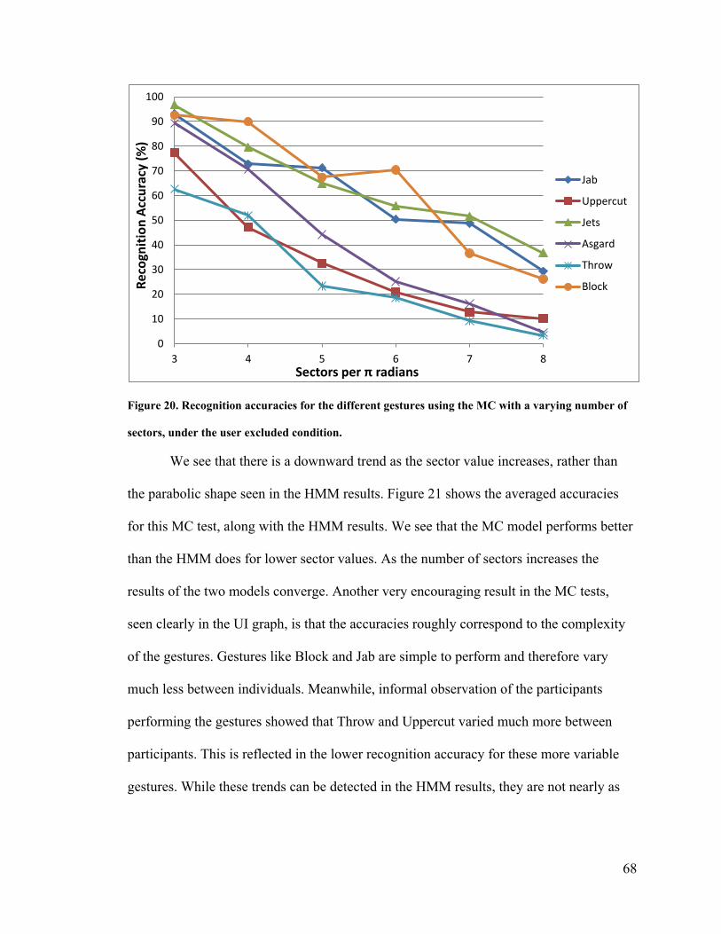
68
Figure 20. Recognition accuracies for the different gestures using the MC with a varying number of
sectors, under the user excluded condition.
We see that there is a downward trend as the sector value increases, rather than
the parabolic shape seen in the HMM results. Figure 21 shows the averaged accuracies
for this MC test, along with the HMM results. We see that the MC model performs better
than the HMM does for lower sector values. As the number of sectors increases the
results of the two models converge. Another very encouraging result in the MC tests,
seen clearly in the UI graph, is that the accuracies roughly correspond to the complexity
of the gestures. Gestures like Block and Jab are simple to perform and therefore vary
much less between individuals. Meanwhile, informal observation of the participants
performing the gestures showed that Throw and Uppercut varied much more between
participants. This is reflected in the lower recognition accuracy for these more variable
gestures. While these trends can be detected in the HMM results, they are not nearly as
0
10
20
30
40
50
60
70
80
90
100
3 4 5 6 7 8
Re
cogn
itio
n A
ccu
racy
(%
)
Sectors per π radians
Jab
Uppercut
Jets
Asgard
Throw
Block
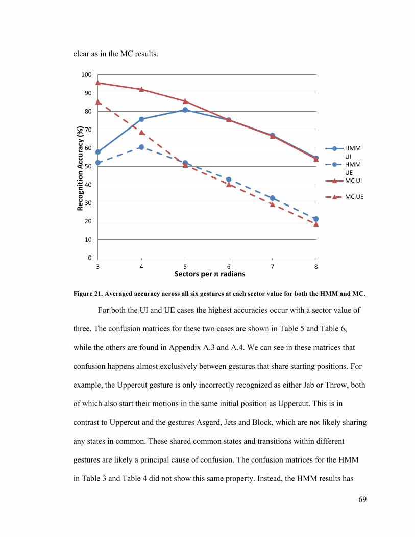
69
clear as in the MC results.
Figure 21. Averaged accuracy across all six gestures at each sector value for both the HMM and MC.
For both the UI and UE cases the highest accuracies occur with a sector value of
three. The confusion matrices for these two cases are shown in Table 5 and Table 6,
while the others are found in Appendix A.3 and A.4. We can see in these matrices that
confusion happens almost exclusively between gestures that share starting positions. For
example, the Uppercut gesture is only incorrectly recognized as either Jab or Throw, both
of which also start their motions in the same initial position as Uppercut. This is in
contrast to Uppercut and the gestures Asgard, Jets and Block, which are not likely sharing
any states in common. These shared common states and transitions within different
gestures are likely a principal cause of confusion. The confusion matrices for the HMM
in Table 3 and Table 4 did not show this same property. Instead, the HMM results has
0
10
20
30
40
50
60
70
80
90
100
3 4 5 6 7 8
Re
cogn
itio
n A
ccu
racy
(%
)
Sectors per π radians
HMM UI HMM UE MC UI
MC UE

70
incorrect recognitions spread across all gestures, regardless of whether they share starting
positions or similar motions.
Looking in the Appendix at the higher sector value matrices, where the two
algorithms converged in overall accuracy, we see that the Markov Chain algorithm's
overall decreasing accuracy leads to an increase in unrecognized gestures. The HMM on
the other hand produces many more incorrectly recognized gestures. Together this
indicates that the Markov Chain algorithm is likely to attribute a false recognition to
either a null recognition, or a gesture which shares elements with the correct gesture. The
HMM algorithm meanwhile, has false recognitions spread across all gestures, without a
strong preference for similar gestures or motions.
Table 5. Confusion matrix for the UI case with the MC algorithm at 3 sector values
Performed Recognized As (%)
Jab Uppercut Jets Asgard Throw Block Unrecognized
Jab 99.6 0.0 0.0 0.0 0.2 0.0 0.2
Uppercut 0.8 91.7 0.0 0.0 2.7 0.0 4.8
Jets 0.0 0.0 99.2 0.0 0.0 0.0 0.8
Asgard 0.0 0.0 0.0 97.1 0.0 0.0 2.9
Throw 3.2 2.0 0.0 0.5 88.2 0.0 6.1
Block 0.0 0.0 0.0 0.5 0.0 98.6 0.9
Table 6. Confusion matrix for the UE case with the MC algorithm at 3 sector values
Performed Recognized As (%)
Jab Uppercut Jets Asgard Throw Block Unrecognized
Jab 93.2 0.0 0.0 0.0 0.2 0.0 6.6
Uppercut 1.2 77.4 0.0 0.0 6.2 0.0 15.2
Jets 0.0 0.0 96.8 0.0 0.0 0.0 3.2
Asgard 0.0 0.0 0.0 89.4 0.0 0.0 10.6
Throw 5.8 5.2 0.0 0.0 62.6 0.0 26.4
Block 0.0 0.0 0.0 1.2 0.0 92.6 6.2

71
6.9 Recognition Time
If we wish to use these recognition algorithms for real-time applications, such as
our active game, the time it takes for the algorithm to recognize the gesture is of critical
importance. As we increase the number of divisions the number of states a given motion
will pass through increases. Figure 22 shows the average times required to parse the
gesture sequence and perform the recognition algorithm for each sector value. All tests
were run on a Windows 7 desktop computer with an Intel i7-3770 3.40GHz CPU and
12 GB of RAM. As would be expected the recognition time increases exponentially with
the number of sectors.
Figure 22. Average computation time for each model to parse and recognize a single test sequence.
From the graph we see that the MC algorithm is faster than the HMM algorithm
across all sector values. The speed differences range from 1.1 times faster than the HMM
at 3 sectors, all the way up to 12.1 times faster at 8 sectors. The times at the lower sector
values are comparable, where the MC achieved higher overall accuracies. At the higher
0
0.05
0.1
0.15
0.2
0.25
0.3
3 4 5 6 7 8
Re
cogn
itio
n T
ime
(se
con
ds)
Segments per π radians
HMM
MC

72
sector values, when the accuracy results converged, the MC algorithm is able to come to
these same results significantly faster than the HMM algorithm.
This is especially important when we incorporate additional sensors into the
recognition system. If we expanded the system to the full 10 sensor system, each sensor
would take approximately equal time for recognition. For the fastest case, MC at 3
sectors, the time per sensor is only 0.00083 seconds. Therefore, the full set of ten sensors
would take less than 10 milliseconds to complete the gesture recognition, even allowing
for a small additional overhead in order to combine the findings of each sensor. This
would allow full body recognition to be performed at approximately 100Hz. This idea
will be discussed more in Section 7.5
It should be noted that the times shown in the graph are averaged across the six
gestures. Some gestures pass through more states than others during their trajectories.
These longer sequences take longer to parse and run through the recognition than the
shorter gesture sequences.
6.10 Modified Markov Chain
Upon examining the individual results of the MC algorithm more closely it was
observed that many of the test sequences that were incorrectly recognized resulted from
probabilities of 0 by the model for the correct gesture. This occurred because the tested
sequence included a transition that was not observed in any of the training data. This is
problematic, as even if all other transitions have very high probabilities, one small
variation can lead to a non-recognition or incorrect classification.
73
We modified the MC algorithm so that rather than assigning a probability of 0 to
any state transition that was not observed in training, the algorithm assigned that
transition a non-zero value. This value should be small enough that it represents an
unlikely transition with respect to the other observed transition probabilities, yet not so
small that on its own will eliminate a gesture from recognition contention.
Several values were tested and in the end we elected to use the value 0.0011. This
value was obtained from the total number of training samples for a given gesture; 450 for
the user excluded case and 490 for the user included case. For a new transition to be seen
in a gesture it must not have been in any of the training sequences and so would occur in
only one of 451 samples. This corresponds to a probability of 0.0022. Some gestures such
as jab may cross through the same state twice, both on the punch forward and pull back.
Therefore, there are twice as many opportunities where a user could have transitioned
into the anomalous state. Hence, we divide our probability value by a factor of two and
obtain our final value of 0.0011.
While this is by no means the definitive best value for this modification, it does
provide easy scalability for different training sample sizes and will continue to reflect the
approximate probability of such a rogue transition occurring. As the number of training
samples increases this value will get smaller and smaller and the results of the regular
MC algorithm will converge towards the results of this Modified Markov Chain. This
value was also fairly insensitive to small (within an order of magnitude) changes of value
and no other number produced notably better results.
It should be noted that by adding this non-zero probability we are violating the
condition that
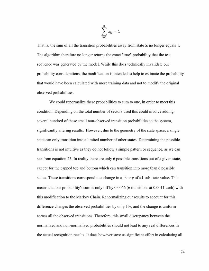
74
That is, the sum of all the transition probabilities away from state Si no longer equals 1.
The algorithm therefore no longer returns the exact "true" probability that the test
sequence was generated by the model. While this does technically invalidate our
probability considerations, the modification is intended to help to estimate the probability
that would have been calculated with more training data and not to modify the original
observed probabilities.
We could renormalize these probabilities to sum to one, in order to meet this
condition. Depending on the total number of sectors used this could involve adding
several hundred of these small non-observed transition probabilities to the system,
significantly altering results. However, due to the geometry of the state space, a single
state can only transition into a limited number of other states. Determining the possible
transitions is not intuitive as they do not follow a simple pattern or sequence, as we can
see from equation 25. In reality there are only 6 possible transitions out of a given state,
except for the capped top and bottom which can transition into more than 6 possible
states. These transitions correspond to a change in α, β or γ of ±1 sub-state value. This
means that our probability's sum is only off by 0.0066 (6 transitions at 0.0011 each) with
this modification to the Markov Chain. Renormalizing our results to account for this
difference changes the observed probabilities by only 1%, and the change is uniform
across all the observed transitions. Therefore, this small discrepancy between the
normalized and non-normalized probabilities should not lead to any real differences in
the actual recognition results. It does however save us significant effort in calculating all
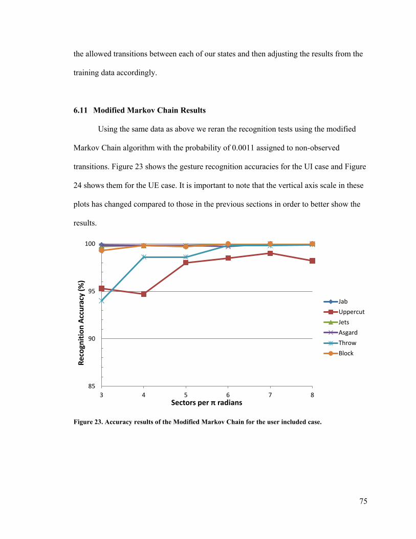
75
the allowed transitions between each of our states and then adjusting the results from the
training data accordingly.
6.11 Modified Markov Chain Results
Using the same data as above we reran the recognition tests using the modified
Markov Chain algorithm with the probability of 0.0011 assigned to non-observed
transitions. Figure 23 shows the gesture recognition accuracies for the UI case and Figure
24 shows them for the UE case. It is important to note that the vertical axis scale in these
plots has changed compared to those in the previous sections in order to better show the
results.
Figure 23. Accuracy results of the Modified Markov Chain for the user included case.
85
90
95
100
3 4 5 6 7 8
Re
cogn
itio
n A
ccu
racy
(%
)
Sectors per π radians
Jab
Uppercut
Jets
Asgard
Throw
Block

76
Figure 24. Accuracy results for the Modified Markov chain for the user excluded case.
As the figures show, this modification to the algorithm has drastically improved
the recognition accuracies of the system. Even for the most difficult case, where the user
has not trained the system in any capacity, the recognition rates for all gestures other than
Throw are above 90% across all sector values. Even with the lowest recognition rate,
Throw still maintains an accuracy over 85%.
The averaged recognition rates are shown in Figure 25. The sector value now has
very little effect on the recognition rates compared to the results of the HMM and MC
algorithms. For the UE case the sector value has almost no effect, with the average
accuracy between 94%-95%. The UI case slowly increases in accuracy with increasing
sector number. Seven sectors had the highest overall accuracies for both conditions and
their confusion matrices are shown in Table 7 and Table 8. The others may be found in
the Appendix A.5 and A.6.
85
90
95
100
3 4 5 6 7 8
Re
cogn
itio
n A
ccu
racy
(%
)
Sectors per π radians
Jab
Uppercut
Jets
Asgard
Throw
Block
77
Figure 25. Accuracy results averaged across all gestures for the Modified Markov Chain
Table 7. Confusion matrix for the Modified Markov Chain for the UI case at seven sectors
Performed Recognized As (%)
Jab Uppercut Jets Asgard Throw Block Unrecognized
Jab 100 0.0 0.0 0.0 0.0 0.0 0.0
Uppercut 0.0 99.0 0.0 0.0 0.5 0.0 0.5
Jets 0.0 0.0 100 0.0 0.0 0.0 0.0
Asgard 0.0 0.0 0.0 100 0.0 0.0 0.0
Throw 0.0 0.0 0.0 0.2 99.8 0.0 0.0
Block 0.0 0.0 0.0 0.0 0.0 100 0.0
85
90
95
100
3 4 5 6 7 8
Re
cogn
itio
n A
ccu
racy
(%
)
Sectors per π radians
Excluded
Included

78
Table 8. Confusion matrix for the Modified Markov Chain for the EU case with seven sectors
Performed Recognized As (%)
Jab Uppercut Jets Asgard Throw Block Unrecognized
Jab 96.0 0.0 0.0 0.8 2.2 1.0 0.0
Uppercut 0.2 92.6 0.4 0.2 6.2 0.0 0.4
Jets 0.0 0.0 99.0 0.4 0.0 0.6 0.0
Asgard 0.4 4.0 0.0 93.4 0.8 1.4 0.0
Throw 2.8 0.2 0.0 7.4 89.6 0.0 0.0
Block 0.0 0.0 0.0 0.8 0.0 99.2 0.0
While we were able to easily modify the Markov Chain algorithm in order to
prevent non-observed transitions from being given a probability of 0, it is not as easy to
replicate this modification in the Hidden Markov Model. The HMM is significantly more
complex, making use of elements like the Baum-Welch and forward-backward
algorithms. Simply setting all non-observed transitions to a non-zero value unfortunately
does not produce meaningful or useful results with this algorithm, as it then allows all
paths between states to become viable routes.
79
7 Chapter: Discussion
7.1 Motion Tracking Performance
As shown by our game demo, the setup we have devised produces a functional
and effective gaming environment. Despite the occasional stutter, as mentioned in
Section 5.10, the motion tracking mirrors the player's movements with a high level of
precision. Lag in the tracking only becomes perceivable when the player makes very
quick and sudden motions. This is likely in part due to the quaternion smoothing we
implemented to reduce jittering. This is an acceptable compensation in our opinion, as we
found this minor delay is not enough to be distracting or break the experience in any way,
whereas the jitter can be very distracting. In the future an empirical test could be devised
to determine a proper balance between the two.
Precision inaccuracies are only apparent when the user can make strong
connections between the virtual and real worlds. Examples of these instances include: the
player touches their hands together in the real world but in the virtual world they are not
quite together or are passing through each other, the player places their arms against their
chest but they pass through the character's chest in-game, or the player reaches to adjust
the Rift and their virtual hands seem too close or far from the virtual head.
These precision issues stem from three main factors. First, while the player will
be close to the character's starting attention pose during calibration they will not be exact,
leading to small precision errors. Similarly, the calibration routine will obtain a very good
approximation of the offset/drift angle, but it will not be perfect. The third significant
factor is that the modeled character is not a perfect replication of the player's body.

80
Attention was given to get the approximate skeletal proportions correct, however for very
fine interactions the exact proportions of arm lengths, shoulder width, etc. are very
important. The culmination of all these small body size differences leads to a disparity
between the virtual and real worlds. Although these accuracy issues exist, they are still
small and for the majority of actions are not immediately apparent to the player.
7.2 Sensor Drift
The most substantial problem with the current system is sensor drift. Some of the
biggest issues have been solved by the implementation of the calibration routine and
allowing the sensors to remain motionless for an initial 13 seconds. Nevertheless, as
Figure 3 showed, the sensors will continue to drift over time. While the drift rate is not
fast enough to be completely prohibitive from play, it does become noticeable to the
player after a few minutes of playing. We implemented a method to apply a counter
rotation into the program to negate this drift, but only obtained mediocre results and so it
was excluded. The somewhat random nature of the drift makes it difficult to counter.
The most obvious and succinct way to solve this issue would be to include
magnetometer data as an additional reference direction. This design has been used in
several other studies and has been shown to resolve the drift issue [57][79]. It is
important to note that this would not eliminate the need for our calibration routine. While
we would no longer be correcting for the sensor's drift through calibration, it is still
needed to orient the sensors' frames with respect to the direction of the screen.

81
7.3 System Scalability
We elected to use a total of ten sensors for our system, allowing us to cover the
major body segments. However, the design of the system is very scalable and can be
easily adjusted for a different number of sensors. For example, adding more sensors to
the feet and hands would provide even more tracking detail and would permit better in-
game walking control. Alternatively, if an application only requires the tracking of the
arms rather than the full skeleton, then this can easily be accommodated, as the
calibration and skeletal model will function equally well, with only minor adjustments.
While the design has been presented as a full body tracking system, it could
accommodate a partial body or expanded body tracking setup equally well.
7.4 Gesture Accuracy
As was seen in our results, our Modified Markov Chain algorithm performed
extremely well when compared to the results of the Hidden Markov Model. It is difficult
to extend these results to compare them directly against other studies. This is due to the
very different conditions between various works, such as a different selection of gestures,
amount of training and number of gestures tested. A recent paper by LaViola [80]
compiled the results across multiple gesture recognition studies, which used a wide
variety of techniques. Based upon the table of results included in their work, most
recognition systems were able to obtain accuracies of over 90%, with an average
accuracy of 93.1% across the studies. Our results compare very favorably to these

82
systems, having obtained average accuracies of between 94%-95% for the user excluded
condition and 98%-100% for the user included condition, depending on the sector value.
7.5 Multiple Gesture Recognition Sensors
Our gesture recognition algorithm uses only a single sensor. We chose to do this
in order to obtain a baseline of the algorithm's capabilities as a gesture recognition system
based on quaternion information, using a Markov based approach. Now that we have
confirmed that this is a viable technique we can expand the recognition system to include
multiple sensors. The increased information provided by additional sensors could result
in higher accuracies and less confusion between gestures.
Of course, having these extra sensors will also cause the computation time to
increase. The recognition time for each sensor should be approximately equal, meaning
that if we were to expand to our full ten sensor system the recognition times should be
approximately ten times those that we found in Figure 22. Even then, the longest
recognition time, at eight sectors, would be less than a quarter of a second in length. The
shortest recognition time, at three sectors, would be just under 0.01 seconds.
It is difficult to determine how the potential accuracy increases from added sensor
information might compare to the extra computation time required by those sensors.
Currently, the highest accuracies (averaged across all six gestures) were obtained at seven
sectors and took on average 0.013 seconds to compute. It is possible that it would be
more efficient to add more sensors and keep the sector number low rather than using a
high sector value. For example, using three sensors at three sectors would take
approximately 3 x 0.0001 seconds, much less than a single sensor at seven sectors.
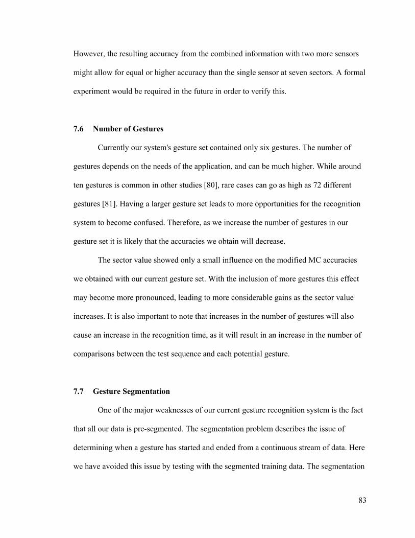
83
However, the resulting accuracy from the combined information with two more sensors
might allow for equal or higher accuracy than the single sensor at seven sectors. A formal
experiment would be required in the future in order to verify this.
7.6 Number of Gestures
Currently our system's gesture set contained only six gestures. The number of
gestures depends on the needs of the application, and can be much higher. While around
ten gestures is common in other studies [80], rare cases can go as high as 72 different
gestures [81]. Having a larger gesture set leads to more opportunities for the recognition
system to become confused. Therefore, as we increase the number of gestures in our
gesture set it is likely that the accuracies we obtain will decrease.
The sector value showed only a small influence on the modified MC accuracies
we obtained with our current gesture set. With the inclusion of more gestures this effect
may become more pronounced, leading to more considerable gains as the sector value
increases. It is also important to note that increases in the number of gestures will also
cause an increase in the recognition time, as it will result in an increase in the number of
comparisons between the test sequence and each potential gesture.
7.7 Gesture Segmentation
One of the major weaknesses of our current gesture recognition system is the fact
that all our data is pre-segmented. The segmentation problem describes the issue of
determining when a gesture has started and ended from a continuous stream of data. Here
we have avoided this issue by testing with the segmented training data. The segmentation

84
problem has been addressed in different ways in the literature. One method is to have the
user hold a controller or other device that allows them to press a button when starting a
gesture and release it when completed. While this is very effective it also requires the
user to be burdened with hand-held devices, which is what we want to avoid with our
gesture-based system.
An alternative is pose-based segmentation. In this solution, the system looks for
specific starting and ending positions and uses them as the segmentation points. While
this is a better alternative for our system than a hand-help controller, it generates a more
pose-based rather than dynamic design. The system then also becomes very dependent on
the user properly starting and ending in those specific poses.
Due to the fast recognition times of our system, it may be possible to perform a
window based recognition approach in real time. This would involve computing multiple
state sequences of differing lengths whenever a new state is added to the state sequence.
Based on our current recognition times, this could allow the system to check multiple
sequence lengths in real time. We could alternatively adopt a dynamic time warping
approach that could act to stretch or compress the state sequences to match similar
characteristics between samples over different time periods. However, this technique can
often be computationally slow [64].
7.8 System Unification
We have successfully managed to create a system that is capable of using a single
set of inertial sensors to perform both body tracking and gesture recognition. Both are
entirely based on the quaternion output of the sensors and we have shown that they have

85
the capability to work in real-time. We currently do not have the two systems operating
simultaneously and to do this one of the first issues to solve would be the segmentation
problem just discussed.
In addition to this, some modifications would need to be made to the gesture
recognition system to unify it with the body tracking system. We are not currently using
the remapped or post-calibration quaternions for the gesture recognition. Both of these
effects are only rotational offsets from our current values. Therefore, they would have no
effect on the actual accuracies that we obtained in our current tests. However, using the
remapped or post-calibration quaternions does mean that the states would be different and
so our current training data would no longer be valid. It is possible that all of the training
data could be modified to reflect the new calibrated/remapped starting positions. For the
current training data the sensor was carefully aligned to be coaxial with the screen. We
could therefore manually apply the necessary rotational offsets to reflect the post-
calibration system. However, we wish to expand the system in the future to utilize
additional sensors in the recognition, which would require the retraining of the gesture
data anyway, so the invalidation of our current training data is not a substantial issue.
Both offsetting the current gesture dataset or recording new data are both fairly
straightforward. The real effort to successfully unify the system will be in finding an
effective solution to the segmentation problem.

86
8 Chapter: Conclusions
8.1 Thesis Findings
In this thesis we have presented a unified motion tracking and gesture recognition
system. Its design is based on the quaternion orientation values output by worn wireless
inertial sensors, each comprised of a three-axis accelerometer and gyroscope. The
development of this system was focused on an active gaming context and a simple game
was developed to demonstrate the capabilities of the motion tracking design.
The motion tracking proved to be an effective method for active gaming input.
The system performed with a high level of accuracy and very low latency, allowing for
an immersive experience. The calibration routine we developed proved to be a successful
way to minimize the drift issues encountered with the inertial sensors. Meanwhile, the
hierarchical skeletal model created for the game character allowed the player to navigate
the virtual environment without the need for controllers or buttons.
Through the robot shooter game we developed, we discovered that this setup was
particularly effective for virtual reality applications. The one-to-one mapping of the
player's motions to the character's actions suited a first-person perspective for gameplay
much better than did a third-person over-the-shoulder view. This was likely due in part to
the shooter style of gameplay, which required a reasonably high level of player precision.
The inclusion of the Oculus Rift added notably to both the experience of the game and
the novelty of the full body control.
In addition to motion tracking, the quaternion output was used for Markov-based
gesture recognition. While the Hidden Markov Model is a very common algorithm used

87
in gesture recognition, the results we obtained show our Modified Markov Chain
performed better than the HMM in both accuracy and computation time. The Modified
Markov Chain achieved an average accuracy of 99% for the user included condition and
an average accuracy of 95% for the more difficult and practical user excluded condition.
These accuracies are comparable to those found in other recognition studies. The
Modified Markov Chain algorithm also had a very fast computation time. At a division
level of three sectors per π radians the recognition algorithm was completed in under a
millisecond, making it an ideal candidate for real-time applications.
8.2 Applications
The focus of the work we have presented here was on full body active gaming and
to a lesser extent virtual reality. Within this gaming concept the sensor network could
expand to include more sensors or shrink to include only the arms or legs as needed.
However, with the rapidly expanding wearable device market and the rise of augmented
and virtual reality, this work could see practical application in a wide variety of contexts.
The motion tracking system could prove useful for applications like remote
physiotherapy [35]. This system could give accurate feedback to patients on how well
they are performing their stretches and exercises without the constant supervision of a
physiotherapist. It could also be used in more general activity monitoring for a wide
range of potential health applications.
The spread of mobile and ubiquitous computing creates an ideal arena for worn
sensor-based gesture recognition. Basic actions on a mobile phone could be completed
without needing to removing it from a pocket. Instead, simple arm or hand gestures could

88
perform these actions. Augmented reality technologies like Google Glass do not have
direct interface methods and instead use primarily a mobile phone or voice interactions,
each of which present their own issues. Worn inertial sensors could allow for a wide
range of hands-free interactions to control applications on such devices through gestures.
8.3 Limitations and Future Work
While this thesis has tackled many of the major issues surrounding the
development of this unified motion tracking and gesture recognition system, there are
still some outstanding issues. One of the most important of these is the handling of the
segmentation problem, which has yet to be addressed. While we did propose that a
windowed approach may be effective based on the fast computation times of the
Modified Markov Chain method, this potential solution needs to be formally tested to
assess its validity and any effects it will have on the recognition accuracy. The gesture
recognition system should also be adapted to work simultaneously with the motion
tracking of the active game. This would allow the game to be expanded to make use of
these extra gesture-based inputs.
While the active game itself is not of key significance to this research, it should be
examined in order to determine the cause of the periodic freezes it encountered. It is
likely an issue with Unity interfacing with the multiple USB ports, but it may also be the
result of one or more sensors behaving improperly.
The sensor drift issue should also be addressed. Acquiring new sensors that have a
magnetometer incorporated into the fusion algorithm would solve this issue. However,
the issue could also potentially be solved with the current sensors. The current sensors do

89
have a magnetometer imbedded into the chip but it is not used for the sensor fusion
algorithm. It is possible that the magnetometer signal could still be utilized to help anchor
the fusion algorithm's quaternion output with the current sensors. Despite these few
remaining issues, this unified motion tracking and gesture recognition system provides a
strong foundation for a wide range of research opportunities and applications in the
future.

90
Appendices
Appendix A Confusion Matrices
Confusion Matrices for all of the gesture recognition results found in Chapter 6.
A.1 HMM User Included
Results for the user excluded Hidden Markov Model discussed in Section 6.6.
3 Sectors
Performed Recognized As (%)
Jab Uppercut Jets Asgard Throw Block Unrecognized
Jab 19.1 0.0 0.2 0.0 0.2 0.0 80.5
Uppercut 1.5 61.8 0.0 0.0 1.0 0.7 35.0
Jets 1.0 0.0 99.0 0.0 0.0 0.0 0.0
Asgard 1.6 0.0 0.0 96.0 0.0 0.5 1.9
Throw 1.8 1.0 0.0 0.0 35.7 1.0 60.5
Block 0.0 0.0 0.0 1.6 0.0 35.6 62.8
4 Sectors
Performed Recognized As (%)
Jab Uppercut Jets Asgard Throw Block Unrecognized
Jab 58.3 0.6 0.1 0.0 0.6 0.0 40.4
Uppercut 2.2 81.6 1.4 0.0 1.4 1.3 12.1
Jets 3.0 0.0 88.3 0.3 0.4 0.0 8.0
Asgard 2.2 0.0 1.1 85.1 0.9 0.2 10.5
Throw 3.9 0.5 3.2 0.0 62.8 3.7 25.9
Block 0.2 0.0 0.5 0.9 0.1 78.6 19.7

91
5 Sectors
Performed Recognized As (%)
Jab Uppercut Jets Asgard Throw Block Unrecognized
Jab 85.6 0.2 1.5 0.0 0.1 0.3 12.3
Uppercut 3.2 72.8 4.1 0.0 3.3 2.9 13.7
Jets 2.3 0.9 86.4 0.8 0.6 1.3 7.7
Asgard 2.6 0.0 4.3 85.3 1.2 1.9 4.7
Throw 4.9 0.2 5.7 0.0 64.7 7.0 17.5
Block 1.6 0.6 0.6 1.9 0.3 90.7 4.3
6 Sectors
Performed Recognized As (%)
Jab Uppercut Jets Asgard Throw Block Unrecognized
Jab 89.8 0.0 1.1 0.0 0.0 2.7 6.4
Uppercut 9.6 63.4 6.6 0.2 2.4 6.7 11.1
Jets 5.2 1.0 84.0 0.2 1.6 3.7 4.3
Asgard 2.6 0.0 4.1 70.8 1.0 11.2 10.3
Throw 5.1 0.1 5.4 0.0 56.1 22.6 10.7
Block 1.8 0.0 1.0 3.7 0.0 88.4 5.1
7 Sectors
Performed Recognized As (%)
Jab Uppercut Jets Asgard Throw Block Unrecognized
Jab 82.3 0.0 2.8 0.0 0.0 4.1 10.8
Uppercut 7.8 53.2 16.8 0.1 5.4 8.9 7.8
Jets 3.9 5.3 80.6 0.9 2.1 2.5 4.7
Asgard 3.0 0.0 14.2 55.0 0.2 16.7 10.9
Throw 12.1 0.0 20.7 0.0 45.7 17.9 3.6
Block 2.2 0.4 2.4 4.1 0.0 84.8 6.1

92
8 Sectors
Performed Recognized As (%)
Jab Uppercut Jets Asgard Throw Block Unrecognized
Jab 74.9 0.1 3.9 0.0 0.0 8.2 12.9
Uppercut 10.7 41.0 18.8 0.0 3.3 15.6 10.6
Jets 6.0 4.8 69.1 0.8 11.3 2.3 5.7
Asgard 7.7 0.0 14.2 34.0 0.1 22.8 21.2
Throw 10.4 0.4 18.8 0.0 30.4 28.8 11.2
Block 0.6 1.1 3.8 4.6 0.0 78.0 11.9
A.2 HMM User Excluded
Results for the user excluded Hidden Markov Model discussed in Section 6.6.
3 Sectors
Performed Recognized As (%)
Jab Uppercut Jets Asgard Throw Block Unrecognized
Jab 19.8 3.4 0.2 0.0 0.2 0.0 76.4
Uppercut 5.8 57.4 0.0 0.0 1.8 2.0 33.0
Jets 2.4 0.0 96.0 0.0 0.0 0.0 1.6
Asgard 4.8 0.0 0.6 81.6 0.0 2.0 11.0
Throw 6.6 2.6 0.4 0.0 23.8 1.2 65.4
Block 1.4 0.0 0.0 2.8 0.0 33.6 62.2
4 Sectors
Performed Recognized As (%)
Jab Uppercut Jets Asgard Throw Block Unrecognized
Jab 48.2 5.4 3.4 0.0 1.4 0.0 41.6
Uppercut 13.8 50.0 2.8 0.0 4.2 5.2 24.0
Jets 10.2 0.2 74.6 0.8 1.8 0.8 11.6
Asgard 8.6 0.0 5.6 68.4 4.0 2.4 11.0
Throw 9.0 1.2 8.0 0.0 43.0 12.8 26.0
Block 1.4 0.0 1.6 1.6 0.2 78.8 16.4

93
5 Sectors
Performed Recognized As (%)
Jab Uppercut Jets Asgard Throw Block Unrecognized
Jab 70.0 0.2 1.2 0.0 2.6 1.2 24.8
Uppercut 11.2 33.6 14.8 0.0 9.0 8.4 23.0
Jets 13.4 6.2 63.8 1.2 2.6 4.8 8.0
Asgard 10.2 0.0 14.0 47.6 4.0 11.2 13.0
Throw 14.4 0.4 16.0 0.0 23.6 14.2 31.4
Block 2.6 3.8 5.6 6.6 1.0 72.8 7.6
6 Sectors
Performed Recognized As (%)
Jab Uppercut Jets Asgard Throw Block Unrecognized
Jab 54.6 0.2 4.0 0.0 0.2 14.8 26.2
Uppercut 24.2 22.0 18.8 0.2 5.4 12.8 16.6
Jets 12.2 3.6 60.2 1.6 4.4 12.0 6.0
Asgard 5.8 0.0 10.8 28.2 4.6 31.4 19.2
Throw 9.2 0.2 19.8 0.0 18.6 32.6 19.6
Block 3.0 0.2 2.8 8.4 0.2 73.8 11.6
7 Sectors
Performed Recognized As (%)
Jab Uppercut Jets Asgard Throw Block Unrecognized
Jab 50.8 0.6 8.6 0.0 0.2 20.0 19.8
Uppercut 9.8 13.4 38.4 0.2 10.8 19.8 7.6
Jets 11.2 12.2 52.8 0.2 9.6 40 10.0
Asgard 8.6 0.0 20.4 17.4 0.4 35.6 17.6
Throw 12.4 0.2 44.2 0.0 10.8 25.4 7.0
Block 10.6 1.2 7.8 6.2 0.4 50.6 23.2
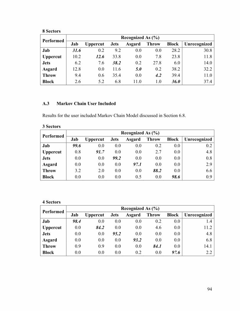
94
8 Sectors
Performed Recognized As (%)
Jab Uppercut Jets Asgard Throw Block Unrecognized
Jab 31.6 0.2 9.2 0.0 0.0 28.2 30.8
Uppercut 10.2 12.6 33.8 0.0 7.8 23.8 11.8
Jets 6.2 7.6 38.2 0.2 27.8 6.0 14.0
Asgard 12.8 0.0 11.6 5.0 0.2 38.2 32.2
Throw 9.4 0.6 35.4 0.0 4.2 39.4 11.0
Block 2.6 5.2 6.8 11.0 1.0 36.0 37.4
A.3 Markov Chain User Included
Results for the user included Markov Chain Model discussed in Section 6.8.
3 Sectors
Performed Recognized As (%)
Jab Uppercut Jets Asgard Throw Block Unrecognized
Jab 99.6 0.0 0.0 0.0 0.2 0.0 0.2
Uppercut 0.8 91.7 0.0 0.0 2.7 0.0 4.8
Jets 0.0 0.0 99.2 0.0 0.0 0.0 0.8
Asgard 0.0 0.0 0.0 97.1 0.0 0.0 2.9
Throw 3.2 2.0 0.0 0.0 88.2 0.0 6.6
Block 0.0 0.0 0.0 0.5 0.0 98.6 0.9
4 Sectors
Performed Recognized As (%)
Jab Uppercut Jets Asgard Throw Block Unrecognized
Jab 98.4 0.0 0.0 0.0 0.2 0.0 1.4
Uppercut 0.0 84.2 0.0 0.0 4.6 0.0 11.2
Jets 0.0 0.0 95.2 0.0 0.0 0.0 4.8
Asgard 0.0 0.0 0.0 93.2 0.0 0.0 6.8
Throw 0.9 0.9 0.0 0.0 84.1 0.0 14.1
Block 0.0 0.0 0.0 0.2 0.0 97.6 2.2
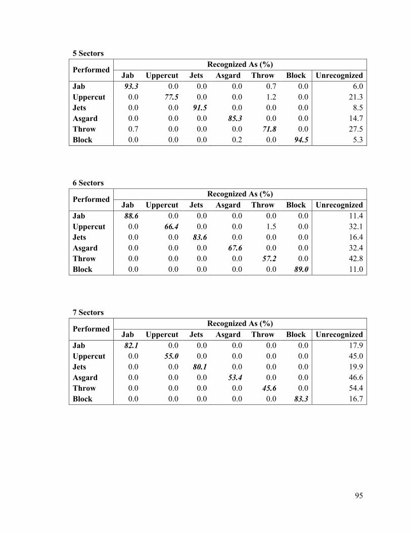
95
5 Sectors
Performed Recognized As (%)
Jab Uppercut Jets Asgard Throw Block Unrecognized
Jab 93.3 0.0 0.0 0.0 0.7 0.0 6.0
Uppercut 0.0 77.5 0.0 0.0 1.2 0.0 21.3
Jets 0.0 0.0 91.5 0.0 0.0 0.0 8.5
Asgard 0.0 0.0 0.0 85.3 0.0 0.0 14.7
Throw 0.7 0.0 0.0 0.0 71.8 0.0 27.5
Block 0.0 0.0 0.0 0.2 0.0 94.5 5.3
6 Sectors
Performed Recognized As (%)
Jab Uppercut Jets Asgard Throw Block Unrecognized
Jab 88.6 0.0 0.0 0.0 0.0 0.0 11.4
Uppercut 0.0 66.4 0.0 0.0 1.5 0.0 32.1
Jets 0.0 0.0 83.6 0.0 0.0 0.0 16.4
Asgard 0.0 0.0 0.0 67.6 0.0 0.0 32.4
Throw 0.0 0.0 0.0 0.0 57.2 0.0 42.8
Block 0.0 0.0 0.0 0.0 0.0 89.0 11.0
7 Sectors
Performed Recognized As (%)
Jab Uppercut Jets Asgard Throw Block Unrecognized
Jab 82.1 0.0 0.0 0.0 0.0 0.0 17.9
Uppercut 0.0 55.0 0.0 0.0 0.0 0.0 45.0
Jets 0.0 0.0 80.1 0.0 0.0 0.0 19.9
Asgard 0.0 0.0 0.0 53.4 0.0 0.0 46.6
Throw 0.0 0.0 0.0 0.0 45.6 0.0 54.4
Block 0.0 0.0 0.0 0.0 0.0 83.3 16.7
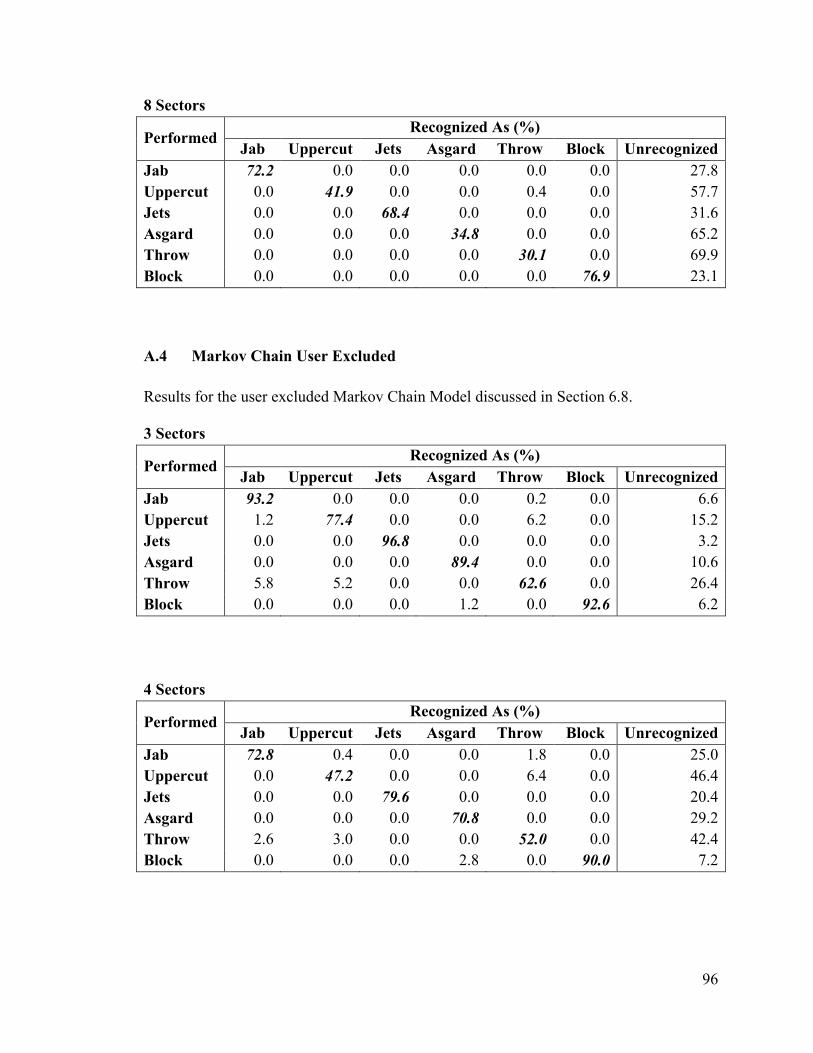
96
8 Sectors
Performed Recognized As (%)
Jab Uppercut Jets Asgard Throw Block Unrecognized
Jab 72.2 0.0 0.0 0.0 0.0 0.0 27.8
Uppercut 0.0 41.9 0.0 0.0 0.4 0.0 57.7
Jets 0.0 0.0 68.4 0.0 0.0 0.0 31.6
Asgard 0.0 0.0 0.0 34.8 0.0 0.0 65.2
Throw 0.0 0.0 0.0 0.0 30.1 0.0 69.9
Block 0.0 0.0 0.0 0.0 0.0 76.9 23.1
A.4 Markov Chain User Excluded
Results for the user excluded Markov Chain Model discussed in Section 6.8.
3 Sectors
Performed Recognized As (%)
Jab Uppercut Jets Asgard Throw Block Unrecognized
Jab 93.2 0.0 0.0 0.0 0.2 0.0 6.6
Uppercut 1.2 77.4 0.0 0.0 6.2 0.0 15.2
Jets 0.0 0.0 96.8 0.0 0.0 0.0 3.2
Asgard 0.0 0.0 0.0 89.4 0.0 0.0 10.6
Throw 5.8 5.2 0.0 0.0 62.6 0.0 26.4
Block 0.0 0.0 0.0 1.2 0.0 92.6 6.2
4 Sectors
Performed Recognized As (%)
Jab Uppercut Jets Asgard Throw Block Unrecognized
Jab 72.8 0.4 0.0 0.0 1.8 0.0 25.0
Uppercut 0.0 47.2 0.0 0.0 6.4 0.0 46.4
Jets 0.0 0.0 79.6 0.0 0.0 0.0 20.4
Asgard 0.0 0.0 0.0 70.8 0.0 0.0 29.2
Throw 2.6 3.0 0.0 0.0 52.0 0.0 42.4
Block 0.0 0.0 0.0 2.8 0.0 90.0 7.2
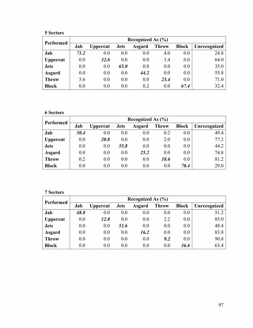
97
5 Sectors
Performed Recognized As (%)
Jab Uppercut Jets Asgard Throw Block Unrecognized
Jab 71.2 0.0 0.0 0.0 4.0 0.0 24.8
Uppercut 0.0 32.6 0.0 0.0 3.4 0.0 64.0
Jets 0.0 0.0 65.0 0.0 0.0 0.0 35.0
Asgard 0.0 0.0 0.0 44.2 0.0 0.0 55.8
Throw 5.6 0.0 0.0 0.0 23.4 0.0 71.0
Block 0.0 0.0 0.0 0.2 0.0 67.4 32.4
6 Sectors
Performed Recognized As (%)
Jab Uppercut Jets Asgard Throw Block Unrecognized
Jab 50.4 0.0 0.0 0.0 0.2 0.0 49.4
Uppercut 0.0 20.8 0.0 0.0 2.0 0.0 77.2
Jets 0.0 0.0 55.8 0.0 0.0 0.0 44.2
Asgard 0.0 0.0 0.0 25.2 0.0 0.0 74.8
Throw 0.2 0.0 0.0 0.0 18.6 0.0 81.2
Block 0.0 0.0 0.0 0.6 0.0 70.4 29.0
7 Sectors
Performed Recognized As (%)
Jab Uppercut Jets Asgard Throw Block Unrecognized
Jab 48.8 0.0 0.0 0.0 0.0 0.0 51.2
Uppercut 0.0 12.8 0.0 0.0 2.2 0.0 85.0
Jets 0.0 0.0 51.6 0.0 0.0 0.0 48.4
Asgard 0.0 0.0 0.0 16.2 0.0 0.0 83.8
Throw 0.0 0.0 0.0 0.0 9.2 0.0 90.8
Block 0.0 0.0 0.0 0.0 0.0 36.6 63.4
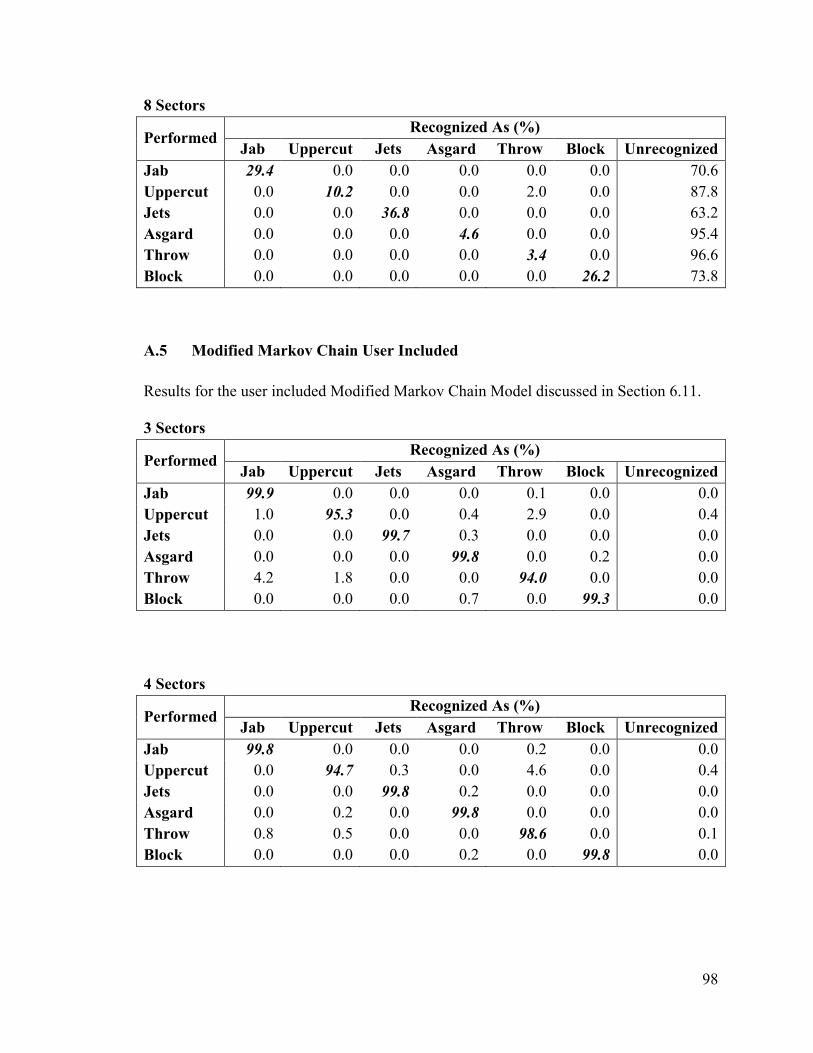
98
8 Sectors
Performed Recognized As (%)
Jab Uppercut Jets Asgard Throw Block Unrecognized
Jab 29.4 0.0 0.0 0.0 0.0 0.0 70.6
Uppercut 0.0 10.2 0.0 0.0 2.0 0.0 87.8
Jets 0.0 0.0 36.8 0.0 0.0 0.0 63.2
Asgard 0.0 0.0 0.0 4.6 0.0 0.0 95.4
Throw 0.0 0.0 0.0 0.0 3.4 0.0 96.6
Block 0.0 0.0 0.0 0.0 0.0 26.2 73.8
A.5 Modified Markov Chain User Included
Results for the user included Modified Markov Chain Model discussed in Section 6.11.
3 Sectors
Performed Recognized As (%)
Jab Uppercut Jets Asgard Throw Block Unrecognized
Jab 99.9 0.0 0.0 0.0 0.1 0.0 0.0
Uppercut 1.0 95.3 0.0 0.4 2.9 0.0 0.4
Jets 0.0 0.0 99.7 0.3 0.0 0.0 0.0
Asgard 0.0 0.0 0.0 99.8 0.0 0.2 0.0
Throw 4.2 1.8 0.0 0.0 94.0 0.0 0.0
Block 0.0 0.0 0.0 0.7 0.0 99.3 0.0
4 Sectors
Performed Recognized As (%)
Jab Uppercut Jets Asgard Throw Block Unrecognized
Jab 99.8 0.0 0.0 0.0 0.2 0.0 0.0
Uppercut 0.0 94.7 0.3 0.0 4.6 0.0 0.4
Jets 0.0 0.0 99.8 0.2 0.0 0.0 0.0
Asgard 0.0 0.2 0.0 99.8 0.0 0.0 0.0
Throw 0.8 0.5 0.0 0.0 98.6 0.0 0.1
Block 0.0 0.0 0.0 0.2 0.0 99.8 0.0

99
5 Sectors
Performed Recognized As (%)
Jab Uppercut Jets Asgard Throw Block Unrecognized
Jab 99.7 0.0 0.0 0.0 0.3 0.0 0.0
Uppercut 0.0 98.0 0.1 0.0 1.5 0.0 0.4
Jets 0.0 0.0 99.8 0.2 0.0 0.0 0.0
Asgard 0.0 0.2 0.0 99.8 0.0 0.0 0.0
Throw 1.4 0.0 0.0 0.0 98.6 0.0 0.0
Block 0.0 0.1 0.0 0.2 0.0 99.7 0.0
6 Sectors
Performed Recognized As (%)
Jab Uppercut Jets Asgard Throw Block Unrecognized
Jab 100 0.0 0.0 0.0 0.0 0.0 0.0
Uppercut 0.0 98.5 0.0 0.0 1.2 0.0 0.3
Jets 0.0 0.0 100 0.0 0.0 0.0 0.0
Asgard 0.0 0.3 0.0 99.7 0.0 0.0 0.0
Throw 0.2 0.0 0.0 0.0 99.8 0.0 0.0
Block 0.0 0.0 0.0 0.0 0.0 100 0.0
7 Sectors
Performed Recognized As (%)
Jab Uppercut Jets Asgard Throw Block Unrecognized
Jab 100 0.0 0.0 0.0 0.0 0.0 0.0
Uppercut 0.0 99.0 0.0 0.0 0.5 0.0 0.5
Jets 0.0 0.0 100 0.0 0.0 0.0 0.0
Asgard 0.0 0.0 0.0 100 0.0 0.0 0.0
Throw 0.0 0.0 0.0 0.2 99.8 0.0 0.0
Block 0.0 0.0 0.0 0.0 0.0 100 0.0

100
8 Sectors
Performed Recognized As (%)
Jab Uppercut Jets Asgard Throw Block Unrecognized
Jab 100 0.0 0.0 0.0 0.0 0.0 0.0
Uppercut 0.0 98.2 0.0 0.0 1.4 0.0 0.4
Jets 0.0 0.0 100 0.0 0.0 0.0 0.0
Asgard 0.0 0.0 0.0 100 0.0 0.0 0.0
Throw 0.1 0.0 0.0 0.0 99.9 0.0 0.0
Block 0.0 0.0 0.0 0.0 0.0 100 0.0
A.6 Modified Markov Chain User Excluded
Results for the user excluded Modified Markov Chain Model discussed in Section 6.11.
3 Sectors
Performed Recognized As (%)
Jab Uppercut Jets Asgard Throw Block Unrecognized
Jab 99.0 0.0 0.0 0.0 1.0 0.0 0.0
Uppercut 1.4 90.6 0.0 0.6 7.0 0.0 0.4
Jets 0.0 0.0 99.4 0.2 0.0 0.4 0.0
Asgard 0.0 1.2 0.0 98.2 0.0 0.6 0.0
Throw 7.8 5.8 0.0 0.0 86.4 0.0 0.0
Block 0.0 0.4 0.0 2.2 0.0 97.4 0.0
4 Sectors
Performed Recognized As (%)
Jab Uppercut Jets Asgard Throw Block Unrecognized
Jab 92.2 0.8 3.0 0.0 4.0 0.0 0.0
Uppercut 0.4 90.6 0.4 0.8 7.4 0.0 0.4
Jets 0.0 0.0 99.6 0.4 0.0 0.0 0.0
Asgard 0.0 1.4 0.2 97.2 0.0 1.2 0.0
Throw 3.8 5.6 0.0 0.0 90.6 0.0 0.0
Block 0.0 0.4 0.0 3.8 0.0 95.8 0.0

101
5 Sectors
Performed Recognized As (%)
Jab Uppercut Jets Asgard Throw Block Unrecognized
Jab 94.8 0.2 0.0 0.2 4.8 0.0 0.0
Uppercut 0.2 91.2 0.6 1.4 6.2 0.0 0.4
Jets 0.0 0.0 99.2 0.4 0.0 0.4 0.0
Asgard 0.0 0.8 0.8 97.2 1.2 0.0 0.0
Throw 7.4 1.2 0.2 1.4 89.8 0.0 0.0
Block 0.0 0.2 0.0 4.0 0.0 95.8 0.0
6 Sectors
Performed Recognized As (%)
Jab Uppercut Jets Asgard Throw Block Unrecognized
Jab 94.4 0.4 0.2 0.6 4.0 0.4 0.0
Uppercut 0.0 92.8 0.6 0.2 6.0 0.0 0.4
Jets 0.0 0.0 98.4 0.4 0.0 1.2 0.0
Asgard 0.4 3.6 1.4 92.2 1.0 1.4 0.0
Throw 3.0 2.4 0.0 5.6 89.0 0.0 0.0
Block 0.0 0.0 0.0 2.8 0.0 97.2 0.0
7 Sectors
Performed Recognized As (%)
Jab Uppercut Jets Asgard Throw Block Unrecognized
Jab 96.0 0.0 0.0 0.8 2.2 1.0 0.0
Uppercut 0.2 92.6 0.4 0.2 6.2 0.0 0.4
Jets 0.0 0.0 99.0 0.4 0.0 0.6 0.0
Asgard 0.4 4.0 0.0 93.4 0.8 1.4 0.0
Throw 2.8 0.2 0.0 7.4 89.6 0.0 0.0
Block 0.0 0.0 0.0 0.8 0.0 99.2 0.0
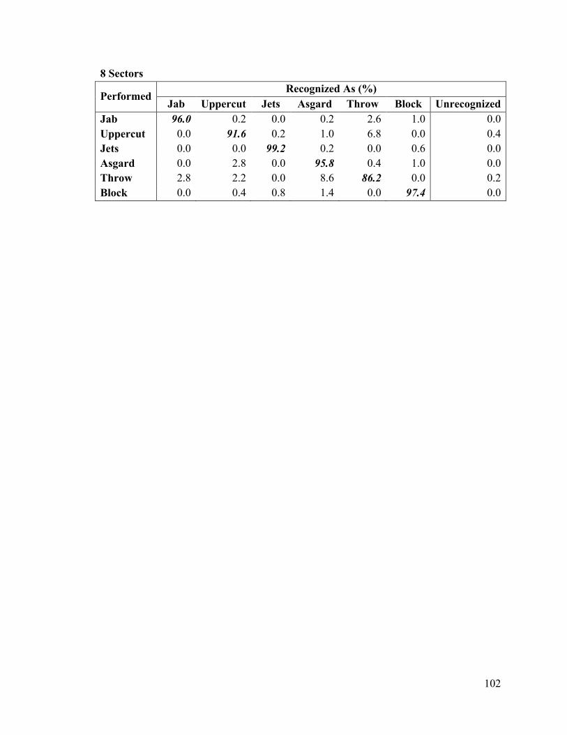
102
8 Sectors
Performed Recognized As (%)
Jab Uppercut Jets Asgard Throw Block Unrecognized
Jab 96.0 0.2 0.0 0.2 2.6 1.0 0.0
Uppercut 0.0 91.6 0.2 1.0 6.8 0.0 0.4
Jets 0.0 0.0 99.2 0.2 0.0 0.6 0.0
Asgard 0.0 2.8 0.0 95.8 0.4 1.0 0.0
Throw 2.8 2.2 0.0 8.6 86.2 0.0 0.2
Block 0.0 0.4 0.8 1.4 0.0 97.4 0.0

103
Bibliography and References
[1] J. Johnson, T. L. Roberts, W. Verplank, D. C. Smith, C. H. Irby, M. Beard, and K.
Mackey, “The Xerox Star : A Retrospective,” Computer (Long. Beach. Calif)., vol.
22, no. 9, pp. 11–26, 1989.
[2] K. Lee, “Wearable tech arrives in full force at CES 2014, but needs to get better,”
TechRadar, 2014. [Online]. Available: http://www.techradar.com/news/portable-
devices/other-devices/wearable-tech-arrives-in-full-force-at-ces-2014-but-needs-
to-get-better-1213971.
[3] “Wearables market hits $6bn,” Ultra Low Power Wireless Q, p. 4.
[4] M. Chen, S. Gonzalez, A. Vasilakos, H. Cao, and V. C. M. Leung, “Body Area
Networks: A Survey,” Mob. Networks Appl., vol. 16, no. 2, pp. 171–193, Aug.
2011.
[5] A. Nijholt, D. O. Bos, and B. Reuderink, “Turning shortcomings into challenges:
Brain–computer interfaces for games,” Entertain. Comput., vol. 1, no. 2, pp. 85–
94, Apr. 2009.
[6] Nintendo, “Wii,” 2014. [Online]. Available: http://wii.com/.
[7] Konami Digital Entertainment, “Dance Dance Revolution,” 2014. [Online].
Available: https://www.konami.com/ddr/.
[8] F. W. Booth, S. E. Gordon, C. J. Carlson, and M. T. Hamilton, “Waging war on
modern chronic diseases: primary prevention through exercise biology,” J. Appl.
Physiol., vol. 88, no. 2, pp. 774–787, 2000.
[9] S. G. Trost, D. Sundal, G. D. Foster, M. R. Lent, and D. Vojta, “Effects of a
Pediatric Weight Management Program With and Without Active Video Games: A
Randomized Trial.,” JAMA Pediatr., Mar. 2014.
[10] Microsoft, “Kinect for Windows,” 2014. [Online]. Available:
http://www.microsoft.com/en-us/kinectforwindows/.
[11] S. Masuko and J. Hoshino, “A fitness game reflecting heart rate,” in Proceedings
of the 2006 ACM SIGCHI international conference on Advances in computer
entertainment technology, 2006, p. 53.
[12] G. Baradoy, “A Physiological Feedback Controlled Exercise Video Game,”
University of Calgary, 2012.

104
[13] K. M. Gilleade, A. Dix, and J. Allanson, “Affective Videogames and Modes of
Affective Gaming : Assist Me , Challenge Me , Emote Me,” in Proceedings of
DiGRA 2005 Conference: Changing Views–Worlds in Play, 2005.
[14] S. I. Hjelm and C. Browall, “Brainball – using brain activity for cool competition,”
in Proceedings of NordiCHI, 2000.
[15] J. A. Pineda, D. S. Silverman, A. Vankov, and J. Hestenes, “Learning to control
brain rhythms: making a brain-computer interface possible,” IEEE Trans. Neural
Syst. Rehabil. Eng., vol. 11, no. 2, pp. 181–184, Jun. 2003.
[16] G. Müller-putz, R. Scherer, and G. Pfurtscheller, “Game-like Training to Learn
Single Switch Operated Neuroprosthetic Control,” in BRAINPLAY 07 Brain-
Computer Interfaces and Games Workshop at ACE (Advances in Computer
Entertainment), 2007, vol. 4, p. 41.
[17] L. E. Nacke, M. Kalyn, C. Lough, and R. L. Mandryk, “Biofeedback Game
Design: Using Direct and Indirect Physiological Control to Enhance Game
Interaction,” in Proceedings of the SIGCHI Conference on Human Factors in
Computing Systems, 2011, pp. 103–112.
[18] K. Kuikkaniemi, T. Laitinen, M. Turpeinen, T. Saari, I. Kosunen, and N. Ravaja,
“The Influence of Implicit and Explicit Biofeedback in First-Person Shooter
Games,” in Proceedings of the SIGCHI Conference on Human Factors in
Computing Systems, ACM, 2010, pp. 859–868.
[19] Oculus VR, “Oculus Rift,” 2014. [Online]. Available:
http://www.oculusvr.com/rift/.
[20] Oculus VR, “Oculus Rift: Step Into the Game,” KickStarter, 2014. [Online].
Available: https://www.kickstarter.com/projects/1523379957/oculus-rift-step-into-
the-game.
[21] Control VR, “Control VR- The Future of Virtual Reality, Animation & More,”
KickStarter, 2014. [Online]. Available:
https://www.kickstarter.com/projects/controlvr/control-vr-motion-capture-for-vr-
animation-and-mor.
[22] Google, “Glass,” 2014. [Online]. Available: https://www.google.com/glass/start/.
[23] D. Comotti, M. Ermidoro, M. Galizzi, and A. Vitali, “Development of a wireless
low-power multi-sensor network for motion tracking applications,” in 2013 IEEE
International Conference on Body Sensor Networks, 2013, pp. 1–6.

105
[24] S. Ullah, H. Higgins, B. Braem, B. Latre, C. Blondia, I. Moerman, S. Saleem, Z.
Rahman, and K. S. Kwak, “A comprehensive survey of wireless body area
networks,” J. Med. Syst., vol. 36, no. 3, pp. 1065–1094, Jun. 2012.
[25] C. Liu, P. Agrawal, N. Sarkar, and S. Chen, “Dynamic Difficulty Adjustment in
Computer Games Through Real-Time Anxiety-Based Affective Feedback,” Int. J.
Hum. Comput. Interact., vol. 25, no. 6, pp. 506–529, Aug. 2009.
[26] R. L. Mandryk, K. M. Inkpen, and T. W. Calvert, “Using psychophysiological
techniques to measure user experience with entertainment technologies,” Behav.
Inf. Technol., vol. 25, no. 2, pp. 141–158, Mar. 2006.
[27] D. Bersak, G. Mcdarby, N. Augenblick, P. Mcdarby, D. Mcdonnell, B. Mcdonald,
and R. Karkun, “Intelligent Biofeedback using an Immersive Competitive
Environment,” in Intelligent biofeedback using an immersive competitive
environment. Paper at the Designing Ubiquitous Computing Games Workshop at
UbiComp., 2001.
[28] A. Dekker and E. Champion, “Please Biofeed the Zombies: Enhancing the
Gameplay and Display of a Horror Game Using Biofeedback,” in Proc. of DiGRA,
2007, pp. 550–558.
[29] A. Bashashati, M. Fatourechi, R. K. Ward, and G. E. Birch, “A survey of signal
processing algorithms in brain-computer interfaces based on electrical brain
signals,” J. Neural Eng., vol. 4, no. 2, pp. R32–57, Jun. 2007.
[30] V. Shnayder, B. Chen, K. Lorincz, T. R. F. Fulford-Jones, and M. Welsh, “Sensor
networks for medical care,” ACM Press, New York, New York, USA, 2005.
[31] A. Whitehead, N. Crampton, K. Fox, and H. Johnston, “Sensor networks as video
game input devices,” in Proceedings of the 2007 conference on Future Play, 2007,
pp. 38–45.
[32] G. Welch and E. Foxlin, “Motion Tracking: No Silver Bullet, but a Respectable
Arsenal,” Comput. Graph. Appl., vol. 22, no. 6, pp. 24–38, 2002.
[33] A. Wood, G. Virone, T. Doan, Q. Cao, L. Selavo, Y. Wu, L. Fang, Z. He, S. Lin,
and J. Stankovic, “ALARM-NET: Wireless Sensor Networks for Assisted-Living
and Residential Monitoring,” 2006.
[34] C. Lai, Y. Huang, J. H. Park, and H.-C. Chao, “Adaptive Body Posture Analysis
for Elderly-Falling Detection with Multisensors,” IEEE Intell. Syst., vol. 25, no. 2,
pp. 20–30, 2010.
[35] K. Kifayat, P. Fergus, S. Cooper, and M. Merabti, “Body Area Networks for
Movement Analysis in Physiotherapy Treatments,” in 2010 IEEE 24th

106
International Conference on Advanced Information Networking and Applications
Workshops, 2010, pp. 866–872.
[36] R. W. Hoyt, J. Reifman, T. S. Coster, and M. J. Buller, “Combat Medical
Informatics : Present and Future Rmtr Triage,” in Proceedings of the AMIA
Symposium, 2002, no. 3, pp. 335–339.
[37] R. W. Hoyt, “SPARNET – Spartan Data Network for Real-Time Physiological
Status Monitoring.” 2008.
[38] A. F. Smeaton, D. Diamond, P. Kelly, K. Moran, D. Morris, N. Moyna, N. E.
O’Connor, and K. Zhang, “Aggregating Multiple Body Sensors for Analysis in
Sports,” in 5th International Workshop on Wearable Micro and Nanosystems for
Personalised Health, 2008.
[39] S. B. Davis, M. Moar, R. Jacobs, M. Watkins, C. Riddoch, and K. Cooke, “‘Ere Be
Dragons: heartfelt gaming,” Digit. Creat., vol. 17, no. 3, pp. 157–162, 2006.
[40] R. De Oliveira and N. Oliver, “TripleBeat: Enhancing Exercise Performance with
Persuasion,” in Proceedings of the 10th international conference on Human
computer interaction with mobile devices and services, 2008, pp. 255–264.
[41] F. Buttussi and L. Chittaro, “Smarter Phones for Healthier Lifestyles: An Adaptive
Fitness Game,” Pervasive Comput. IEEE, vol. 9, no. 4, pp. 51–57, 2010.
[42] H. Johnston and A. Whitehead, “Pose presentation for a dance-based massively
multiplayer online exergame,” Entertain. Comput., vol. 2, no. 2, pp. 89–96, Jan.
2011.
[43] A. Whitehead, H. Johnston, K. Fox, N. Crampton, and J. Tuen, “Homogeneous
accelerometer-based sensor networks for game interaction,” Comput. Entertain.,
vol. 9, no. 1, p. 1, Apr. 2011.
[44] E. Charbonneau, A. Miller, C. A. Wingrave, and J. J. LaViola Jr, “Poster:
RealDance: An Exploration of 3D Spatial Interfaces for Dancing,” in IEEE
Symposium on 3D User Interfaces, 2009, pp. 141–142.
[45] A. Kailas, “Basic human motion tracking using a pair of gyro + accelerometer
MEMS devices,” in IEEE 14th International Conference on e-Health Networking,
Applications and Services, 2012, no. 1, pp. 298–302.
[46] C. Yang, J. Hu, C. Yang, C. Wu, and N. Chu, “Dancing game by digital textile
sensor, accelerometer and gyroscope,” in 2011 IEEE International Games
Innovation Conference (IGIC), 2011, pp. 121–123.
107
[47] C.-H. Wu, Y.-T. Chang, and Y.-C. Tseng, “Multi-screen cyber-physical video
game: An integration with body-area inertial sensor networks,” in 2010 8th IEEE
International Conference on Pervasive Computing and Communications
Workshops (PERCOM Workshops), 2010, pp. 832–834.
[48] K. Zintus-art, S. Saetia, V. Pongparnich, and S. Thiemjarus, “Dogsperate Escape:
A demonstration of real-time BSN-based game control with e-AR sensor,” in
Knowledge, Information, and Creativity Support Systems, vol. 6746, Berlin
Heidelberg: Springer, 2011, pp. 253–262.
[49] B. Mortazavi, K. C. Chu, X. Li, J. Tai, S. Kotekar, and M. Sarrafzadeh, “Near-
realistic motion video games with enforced activity,” in 2012 Ninth International
Conference on Wearable and Implantable Body Sensor Networks, 2012, pp. 28–
33.
[50] S. Kim and M. A. Nussbaum, “Performance evaluation of a wearable inertial
motion capture system for capturing physical exposures during manual material
handling tasks.,” Ergonomics, vol. 56, no. 2, pp. 314–326, Jan. 2013.
[51] E. Farella, L. Benini, B. Riccò, and A. Acquaviva, “MOCA: A low-power, low-
cost motion capture system based on integrated accelerometers,” Adv. Multimed.,
vol. 2007, no. 1, pp. 1–1, 2007.
[52] Z.-Q. Zhang, W.-C. Wong, and J.-K. Wu, “Ubiquitous human upper-limb motion
estimation using wearable sensors.,” IEEE Trans. Inf. Technol. Biomed., vol. 15,
no. 4, pp. 513–21, Jul. 2011.
[53] Z.-Q. Zhang, L.-Y. Ji, Z.-P. Huang, and J.-K. Wu, “Adaptive Information Fusion
for Human Upper Limb Movement Estimation,” IEEE Trans. Syst. Man, Cybern. -
Part A Syst. Humans, vol. 42, no. 5, pp. 1100–1108, Sep. 2012.
[54] H. J. Luinge and P. H. Veltink, “Measuring orientation of human body segments
using miniature gyroscopes and accelerometers,” Med. Biol. Eng. Comput., vol.
43, no. 2, pp. 273–82, Mar. 2005.
[55] H. J. Luinge, P. H. Veltink, and C. T. M. Baten, “Ambulatory measurement of arm
orientation,” J. Biomech., vol. 40, no. 1, pp. 78–85, Jan. 2007.
[56] C. M. N. Brigante, N. Abbate, A. Basile, A. C. Faulisi, and S. Sessa, “Towards
Miniaturization of a MEMS-Based Wearable Motion Capture System,” IEEE
Trans. Ind. Electron., vol. 58, no. 8, pp. 3234–3241, Aug. 2011.
[57] E. R. Bachmann, “Inertial and magnetic angle tracking of limb segments for
inserting humans into sythetic environments,” Naval Postgraduate School, 2000.

108
[58] Xsens, “Xsens MVN,” 2014. [Online]. Available:
http://www.xsens.com/products/xsens-mvn/.
[59] N. C. Krishnan and S. Panchanathan, “Body Sensor Networks for Activity and
Gesture Recognition,” in The Art of Wireless Sensor Networks, H. M. Ammari, Ed.
Berlin, Heidelberg: Springer Berlin Heidelberg, 2014, pp. 567–605.
[60] N. Ravi, N. Dandekar, P. Mysore, and M. L. Littman, “Activity Recognition from
Accelerometer Data,” Am. Assoc. Artif. Intell., vol. 5, pp. 1541–1546, 2005.
[61] S. Zhou, Z. Dong, J. Li, Wen, and P. Kwong, Chung, “Hand-written character
recognition using MEMS motion sensing technology,” in 2008 IEEE/ASME
International Conference on Advanced Intelligent Mechatronics, 2008, pp. 1418–
1423.
[62] J. Yang, E.-S. Choi, W. Chang, W.-C. Bang, S.-J. Cho, J.-K. Oh, J.-K. Cho, and
D.-Y. Kim, “A novel hand gesture input device based on inertial sensing
technique,” in Industrial Electronics Society, 2004. 30th Annual Conference of
IEEE. Vol. 3, 2004, pp. 2786–2791.
[63] P. Trindade and J. Lobo, “Distributed Accelerometers for Gesture Recognition and
Visualization,” in Technological Innovation for Sustainability, no. 231640, 2011,
pp. 215–223.
[64] H. C. Jian, “Gesture Recognition Using Windowed Dynamic Time Warping,”
National University of Singapore, 2010.
[65] L. Kratz, M. Smith, and F. J. Lee, “Wiizards : 3D Gesture Recognition for Game
Play Input,” in Proceedings of the 2007 conference on Future Play, 2007, pp. 209–
212.
[66] J. Mäntyjärvi, J. Kela, P. Korpipää, and S. Kallio, “Enabling fast and effortless
customisation in accelerometer based gesture interaction,” in Proceedings of the
3rd international conference on Mobile and ubiquitous multimedia, 2004, pp. 25–
31.
[67] J. Kela, P. Korpipää, J. Mäntyjärvi, S. Kallio, G. Savino, L. Jozzo, and S. Di
Marca, “Accelerometer-based gesture control for a design environment,” Pers.
Ubiquitous Comput., vol. 10, no. 5, pp. 285–299, Aug. 2005.
[68] A. D. Whitehead, “Gesture Recognition with Accelerometers for Game
Controllers, Phones and Wearables,” GSTF Int. J. Comput., vol. 3, no. 4, pp. 63–
69, 2014.
109
[69] M. Chen, G. AlRegib, and B. Juang, “Feature processing and modeling for 6D
motion gesture recognition,” IEEE Trans. Multimed., vol. 15, no. 3, pp. 561–571,
2013.
[70] Microchip, “Motion sensing demo board,” 2014. [Online]. Available:
http://www.microchip.com/motion.
[71] InvenSense, “MPU-6000/6050 six-axis MEMS MotionTracking decivces,” 2014.
[Online]. Available: http://www.invensense.com/mems/gyro/mpu6050.html.
[72] X. Yun and E. R. Bachmann, “Design, Implementation, and Experimental Results
of a Quaternion-Based Kalman Filter for Human Body Motion Tracking,” IEEE
Trans. Robot., vol. 22, no. 6, pp. 1216–1227, Dec. 2006.
[73] G. Welch and G. Bishop, “An Introduction to the Kalman Filter,” in Proc of
SIGGRAPH, Course 8, 2001, pp. 27599–3175.
[74] R. Mukundan, “Quaternions : From classical mechanics to computer graphics , and
beyond,” in Proceedings of the 7th Asian Technology Conference in Mathematics,
2002.
[75] Unity, “Unity,” 2014. [Online]. Available: http://unity3d.com/.
[76] “WinUSBNet,” Google Code, 2012. [Online]. Available:
https://code.google.com/p/winusbnet/.
[77] L. R. Rabiner, “A tutorial on hidden Markov models and selected applications in
speech recognition,” Proc. IEEE, vol. 77, no. 2, pp. 257–286, 1989.
[78] J. Diebel, “Representing Attitude : Euler Angles , Unit Quaternions , and Rotation
Vectors. Technical Report,” Palo Alto, CA, 2006.
[79] R. Zhu and Z. Zhou, “A real-time articulated human motion tracking using tri-axis
inertial/magnetic sensors package.,” IEEE Trans. Neural Syst. Rehabil. Eng., vol.
12, no. 2, pp. 295–302, Jun. 2004.
[80] J. J. LaViola Jr, “3D Gestural Interaction : The State of the Field,” ISRN Artif.
Intell., vol. 2013, p. 18, 2013.
[81] X. Zhang, X. Chen, Y. Li, V. Lantz, K. Wang, and J. Yang, “A Framework for
Hand Gesture Recognition Based on Accelerometer and EMG Sensors,” IEEE
Trans. Syst. Man Cybern. Part A Syst. Humans, vol. 41, no. 6, pp. 1064–1076,
2011.