A RATIONAL APPROXIMATION METHOD FOR SOLVINGACOUSTIC NONLINEAR EIGENVALUE PROBLEMS

MOHAMED EL-GUIDE ∗, AGNIESZKA MIEDLAR † , AND YOUSEF SAAD ‡

Abstract. We present two approximation methods for computing eigenfrequencies and eigen-modes of large-scale nonlinear eigenvalue problems resulting from boundary element method (BEM)solutions of some types of acoustic eigenvalue problems in three-dimensional space. The main ideaof the first method is to approximate the resulting boundary element matrix within a contour inthe complex plane by a high accuracy rational approximation using the Cauchy integral formula.The second method is based on the Chebyshev interpolation within real intervals. A Rayleigh-Ritzprocedure, which is suitable for parallelization is developed for both the Cauchy and the Chebyshevapproximation methods when dealing with large-scale practical applications. The performance ofthe proposed methods is illustrated with a variety of benchmark examples and large-scale industrialapplications with degrees of freedom varying from several hundred up to around two million.

Key words. nonlinear eigenvalue problem, boundary element method, rational approximation,Cauchy integral formula

1. Background and Introduction. The Boundary Element Method (BEM) isa powerful approach developed to solve integral equations [16]. The idea of applyingthe BEM in many branches of science and engineering has gained popularity over thepast few years, e.g., in elasticity, ground and water flow, wave propagation and inelectromagnetic problems [19]. The most commonly used approaches for numericallysolving PDEs are the Finite Difference Method (FDM) and the Finite Element Method(FEM). A standard finite difference method is suitable when dealing with simpledomains (e.g. rectangular grids), while the finite element method can handle morecomplex domains. However, much work has to be done to numerically dicretize awhole computational domain (generate meshes) and this task becomes even moredifficult when dealing with complicated domains in higher dimensions, i.e., d ≥ 3. Thisis where BEM becomes appealing because it allows to significatly reduce the overallcomputational complexity of the solution process. Instead of solving a problem for thepartial differential operator defined on the whole domain Ω, the boundary elementmethod uses an associated boundary integral equation reducing the domain of theproblem to the boundary ∂Ω. This comes at a cost since the matrix problem to solvein the approximation becomes dense.

In the following, we are interested in the efficient solution of nonlinear eigenvalueproblems (NLEVPs) resulting from the boundary element (BE) discertization of theacoustic problems. Although a finite element discretization of the problem yields ageneralized (linear) eigenvalue problem, it requires a discretization of the whole do-main Ω which is not always feasible, e.g., if the domain is unbounded. Though thetopic of NLEVPs built upon the boundary element method (BEM) has been aroundfor a number of years, the lack of efficient eigensolvers has delayed a full exploration

∗International Water Research Institute, Mohammed VI Polytechnic University, Green City, Mo-rocco and University of Minnesota, Department of Computer Science & Engineering, 4-192 KellerHall, 200 Union Street SE, Minneapolis, MN 55455, USA. Work supported by NSF grant 1812695.e-mail: mohamed.elguide@um6p.ma†University of Kansas, Department of Mathematics, 405 Snow Hall, 1460 Jayhawk Blvd.

Lawrence, KS 66045-7594, USA. Work supported by NSF grant 1812927. e-mail: amiedlar@ku.edu‡University of Minnesota, Department of Computer Science & Engineering, 4-192 Keller Hall, 200

Union Street SE, Minneapolis, MN 55455, USA. Work supported by NSF grant 1812695. e-mail:saad@umn.edu

1

arX

iv:1

906.

0393

8v1

[m

ath.

NA

] 7

Jun

201

9

of BE–based approaches. Recently, eigenvalue solvers based on contour integrals weredeveloped and this made BEM an attractive alternative to the usual contenders whensolving challenging nonlinear eigenvalue problems [15, 22, 23]. Contour based meth-ods have the ability to solve NLEVPs when the eigenvalues of interest lie inside agiven closed contour in the complex plane using rational or polynomial approxima-tion [7, 9, 4, 21, 13]. Despite these efforts, solving NLEVPs is still a computationallyintensive task. Assembling interpolation matrices and solving linear systems in theBE framework are already very expensive due to the unstructured, dense and com-plex nature of the resulting matrices. For example, the Chebyshev interpolation ofthe BE formulation of the large-scale accoustic problem discussed in [7] results ina generalized eigenvalue problem which cannot be easily handled with the state-of-the-art linear solvers. Another drawback of this method is that the quality of theapproximations quickly deteriorates when dealing with complex eigenvalues.

It is the purpose of this paper to overcome the aforementioned difficulties anddevelop eigensolvers suitable for calculations of eigenvalues of NLEVPs arbitrarly lo-cated in the complex plane. The paper illustrates the performance of the proposedmethod with a problem that arises in the modal analysis of large-scale acoustic prob-lems.

Consider the three-dimensional (3D) acoustic Helmholtz equation

∆u(x) + k2u(x) = 0, x ∈ Ω ⊂ R3, (1.1)

where ∆ is the Laplace operator, u(x) is the sound pressure at point x, k = ω/c isthe wave number with the circular frequency ω and the speed of sound c through thefluid medium. Equation (1.1) is subject to a homogeneous condition on its boundary∂Ω of the form

a(x)u(x) + b(x)∂u(x)

∂n= 0, x ∈ ∂Ω, (1.2)

where ∂∂n denotes the outward normal to the boundary at point x.

Using BEM yields the following Helmholtz integral equation [11]

C(x)u(x) =

∫∂Ω

(∂g

∂nyu(y)− g(‖x− y‖) ∂u

∂ny

)dy, (1.3)

where C denotes the solid angle at point x, ny the surface unit normal vector at pointy and g(·) the free-space Green’s function [6, 3]

g(‖x− y‖) =eiz‖x−y‖

4π‖x− y‖. (1.4)

The continuous Helmholtz integral equation (1.3) can be discretized to form the fol-lowing discrete problem from which the unknown boundary node values z can bedetermined,

T (z)u = 0, T (z) := AH(z)−BG(z), (1.5)

where A and B are diagonal matrices related to the functions a(·) and b(·) in (1.2), HandG are the matrices containing the coefficients related to the integrals on the surfaceof ∂g

∂nyand g, respectively [11]. The boundary integrals are discretized by Gauss-

Legendre quadrature where the singularities of Green’s function and its derivative are

2

isolated in the integral of revolution, and the integrations are performed analyticallyusing sums of elliptic integrals [12]. Here, T (z) ∈ Cn×n is a matrix function that isnonlinear is z and holomorphic since the free-space Green’s functions are holomorphicfunctions of z. Obviously, equation (1.5) is a NLEVP of the general form

T (λ)u = 0, (1.6)

and the objective of this paper is to develop methods for finding all eigenvalues z,satisfying (1.5), that are located inside a certain region of the complex plane enclosedby the contour Γ.

2. Rational and Chebyshev approximation methods for NLEVPs. Thefirst method we consider is adapted from [14] and it is based on the Cauchy’s integralformula. Given a Jordan curve Γ that surrounds the eigenvalues of interest, we expressthe matrix function T (z) as follows:

T (z) =1

2ıπ

∫Γ

T (t)

t− zdt. (2.1)

By replacing both occurrences of T (·) in (2.1) by Tij(·), one can see that the aboveexpression is equivalent to expressing each individual entry Tij(z) of T (z) by theCauchy integral formula. Equality (2.1) is valid for z inside the contour Γ and theonly requirement is that T (z) be analytic inside the contour. As is classically done[10] we use a numerical quadrature formula to obtain the following Cauchy integral

approximation T (z) of T (z)

T (z) ≈m∑i=0

ωiT (σi)

z − σi, (2.2)

where the σi’s are quadrature points located on the contour Γ and the ωi’s the corre-sponding quadrature weights.

Setting Bi = ωiT (σi), equation (2.2) can be rewritten as

T (z) =B0

z − σ0+

B1

z − σ1+ . . .+

Bmz − σm

, (2.3)

= B0f0(z) +B1f1(z) + . . .+Bmfm(z), (2.4)

with fi(z) = 1z−σi

, i = 0, . . . ,m. For a given vector u we now define

vi := fi(z)u, for i = 0, . . . ,m.

Then the approximate nonlinear eigenvalue problem T (z)u = 0 yields

T (z)u = B0v0 +B1v1 + . . .+Bmvm = 0. (2.5)

Chebyshev interpolation of order m can also be used to obtain the same formas (2.4) of the approximation of the matrix-valued function T (z). In this method,proposed in [7], the function T (z) is expanded using a degree m Chebyshev polynomialexpansion of the form [1] :

T (z) = B0τ0(z) +B1τ1(z) + . . .+Bmτm(z), (2.6)

3

where Bi and τi(z) are coefficient matrices and Chebyshev basis functions, respec-tively. The corresponding nonlinear eigenvalue problem is of the same form as (2.5)with the vectors vi now defined by vi = τi(z)u.

The problem (2.5) for the Cauchy interpolation, and its Chebyshev interpolationcounterpart, can be reformulated as a generalized linear eigenvalue problem:

Aw = λMw. (2.7)

For the Cauchy rational approximation we have:

A =

σ0I I

σ1I I. . .

...σmI I

−B0 −B1 · · · −Bm 0

, M =

II

. . .

. . .

0

, (2.8)

and w =[vT0 , v

T1 , . . . , v

Tm, u

T]T

whereas for the Chebyshev interpolation

A =

0 II 0 I

. . .. . .

. . .

I 0 I−B0 · · · −Bm−3 Cm−2 −Bm−1

, M = 2

12I

I

. . .

IBm

, (2.9)

where Cm−2 ≡ Bm −Bm−2 and w =[uT , vT1 , . . . , v

Tm−1, v

Tm

]T.

With regards to the rational approximation described above, we note that analternative that has been used with some success in the literature is the Barycen-tric approximation formula [4]. However, our tests with this technique showed nosignificant improvement in our context over the simple Cauchy formula used above.Note that it is also possible to exploit other polynomials, using different classes of or-thogonal polynomials but we will restrict our attention to Chebyshev polynomials ofthe first kind. Finally note that Chebyshev approximation works best for eigenvalueslocated in an interval while the Cauchy rational approximation is suitable for generalcomplex spectra.

3. Rayleigh–Ritz procedure for BEM eigenvalue problem. Let U be abasis of dimension ν of a subspace that contains good approximations of the eigen-vectors of the NLEVP problem (1.5). Then, it is possible to apply a Rayleigh-Ritzprocedure to (1.5) to obtain approximate eigenpairs. The approximate eigenvectorwill be of the form u = Uy with y ∈ Cν . Then expressing that T (z)u is orthogonalto the range of U yields the projected problem UHTU (z)u = 0 or,

B0f0(z)y + B1f1(z)y + . . .+ Bmfm(z)y = 0, (3.1)

where Bi = UHBiU . We will denote TU (z) the projected operator, namely,

TU (z) = B0f0(z) + B1f1(z) + . . .+ Bmfm(z). (3.2)

Then, applying the same procedure as before to the projected problem we seethat (3.1) becomes:

B0v0 + B1v1 + . . .+ Bmvm = 0, (3.3)

with vi = yz−σi

in the case of rational approximation and vi = τi(z)y when a Rayleigh-Ritz procedure is applied to the Chebyshev interpolation.

4

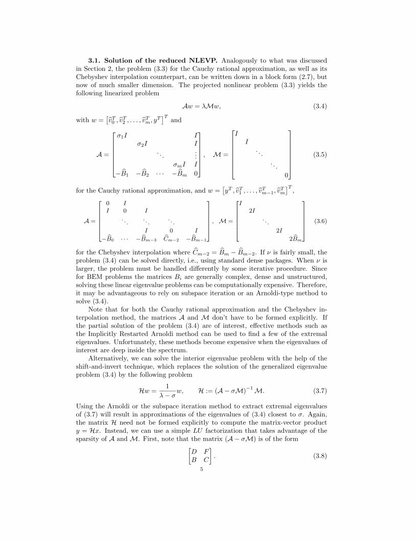
3.1. Solution of the reduced NLEVP. Analogously to what was discussedin Section 2, the problem (3.3) for the Cauchy rational approximation, as well as itsChebyshev interpolation counterpart, can be written down in a block form (2.7), butnow of much smaller dimension. The projected nonlinear problem (3.3) yields thefollowing linearized problem

Aw = λMw, (3.4)

with w =[vT0 , v

T2 , . . . , v

Tm, y

T]T

and

A =

σ1I I

σ2I I. . .

...σmI I

−B1 −B2 · · · −Bm 0

, M =

II

. . .

. . .

0

(3.5)

for the Cauchy rational approximation, and w =[yT , vT1 , . . . , v

Tm−1, v

Tm

]T,

A =

0 II 0 I

. . .. . .

. . .

I 0 I

−B0 · · · −Bm−3 Cm−2 −Bm−1

, M =

I

2I

. . .

2I

2Bm

(3.6)

for the Chebyshev interpolation where Cm−2 = Bm − Bm−2. If ν is fairly small, theproblem (3.4) can be solved directly, i.e., using standard dense packages. When ν islarger, the problem must be handled differently by some iterative procedure. Sincefor BEM problems the matrices Bi are generally complex, dense and unstructured,solving these linear eigenvalue problems can be computationally expensive. Therefore,it may be advantageous to rely on subspace iteration or an Arnoldi-type method tosolve (3.4).

Note that for both the Cauchy rational approximation and the Chebyshev in-terpolation method, the matrices A and M don’t have to be formed explicitly. Ifthe partial solution of the problem (3.4) are of interest, effective methods such asthe Implicitly Restarted Arnoldi method can be used to find a few of the extremaleigenvalues. Unfortunately, these methods become expensive when the eigenvalues ofinterest are deep inside the spectrum.

Alternatively, we can solve the interior eigenvalue problem with the help of theshift-and-invert technique, which replaces the solution of the generalized eigenvalueproblem (3.4) by the following problem

Hw =1

λ− σw, H := (A− σM)

−1M. (3.7)

Using the Arnoldi or the subspace iteration method to extract extremal eigenvaluesof (3.7) will result in approximations of the eigenvalues of (3.4) closest to σ. Again,the matrix H need not be formed explicitly to compute the matrix-vector producty = Hx. Instead, we can use a simple LU factorization that takes advantage of thesparsity of A and M. First, note that the matrix (A− σM) is of the form[

D FB C

]. (3.8)

5

By exploiting the sparsity of the matrices D and F , we can easily form the followingLU factorization

L =

[I 0

BD−1 I

], U =

[D F0 S

], (3.9)

where S = C − BD−1F is known as the Schur complement of the block C. Withthe use of matrix S, we can use the Arnoldi algorithm on vectors of shorter length.Solving the shifted and inverted problem (3.7) with Arnoldi algorithm requires solvinglinear systems of the form [

D FB C

] [xy

]=

[ab

]. (3.10)

Using the Schur complement S, y can be easily obtained by solving Sy = b−BD−1aand since D is a diagonal matrix and F is a block of identity matrices, one candetermine x by using the relation Dx+ Fy = a.

3.2. Construction of the subspace of approximants. We begin this sec-tion by noting that the Arnoldi-type or subspace iteration methods discussed in theprevious section can be applied to a linear eigenvalue problem Aw = λMw obtaineddirectly from (2.5). However, proceeding in this way would require either solving lin-ear eigenvalue problems of size mn+ n when using Arnoldi-type methods, or storingvectors of length mn+n in the subspace iteration method, and this can be computa-tionally expensive when m is large. Therefore, it is important to develop a techniquethat allows to work with subspaces of smaller dimensions that requires storing shortervectors. A procedure of this type, which works with subspaces of dimention m is pre-sented next.

Let us first consider a large linear eigenproblem of the form (2.7) obtained from(2.5) without a projection. To introduce the approach that works with vectors ofdimension n, we first point out that for an approximate eigenpair (λ, u), u is thebottom (resp. top part) of an approximate eigenvector w of the large linear eigenvalueproblem (2.7) associated with (2.4) for the Cauchy rational approximation, (resp.(2.6) for the Chebyshev interpolation). Let W (0) be a random initial set of ν basisvectors of a certain subspace, where each of the ν columns is of the form 1 w = [v;u](resp. w = [u; v]) for the splitting associated with the Cauchy rational approximation(resp. Chebyshev interpolation). Next, in order to make these initial random vectorsclose to the eigenvectors of interest, we apply q steps of the inverse power methodwith matrix H in (3.7) to each column of W (0) separately. A subspace of dimensionn that approximates the eigenvectors of (2.5) is then obtained from the bottom parts(resp. top parts) of the processed columns for the Cauchy rational approximation(rep. Chebyshev interpolation). Although this process involves the column vectors ofW (0), only vectors of length n need to be saved and the iterates v can be discarded.The accuracy of the extracted eigenpairs obtained from applying a Rayleigh-Ritzprojection can be further refined by updating U in a process that takes advantage ofthe structure of the approximate eigenvectors. Let (λ, u) be an approximate eigenpairof (2.5) obtained from applying a Rayleigh-Ritz projection using U . The new redefinedvector w for each interpolation method is discussed next. For the Cauchy rationalapproximation, the vector v = [v1; v2; ...; vm]T (the top part of vector w), is obtainedby setting vi = u

λ−σi, whereas for the Chebyshev interpolation (the bottom part of

vector w) it is defined by setting vi = τi(λ)u.

1Here we use Matlab notation: [v;u] is a vector that stacks v on top of u.

6

3.3. The inverse power method. The straightforward linearizations (2.8) ofthe Cauchy rational approximation and (2.9) of the Chebyshev interpolation, dis-cussed in Section 2, are high dimensional problems and they become computationallydemanding as the order m of the approximations grows. The Rayleigh-Ritz approachdiscussed above is inexpensive even if m is large. The biggest computational taskof the presented Rayleigh-Ritz projection lies in performing q steps of the inversepower method with the matrix (A− σM)

−1M. It is the purpose of the followingdiscussion to show how each step of the inverse power method can be carried outinexpensively. For simplicity, we will assume that the shift σ is the center of the unitcircle (resp. interval [−1, 1]) for the Cauchy rational approximation (resp. Chebyshevinterpolation). This is a natural choice, since any circle in the complex plane canbe scaled to the unit circle and any real interval [a, b] can be scaled to the interval[−1, 1]. Throughout this discussion, the superscript j will correspond to the iterationnumber, while the subscript i will correspond to the blocks of the vectors v(j). Webegin by discussing the inverse power method for the Cauchy rational approximation.

Inverse power iteration for the Cauchy rational approximation. For the Cauchyinterpolation, each step of the inverse power iteration method requires solving a linearsystem

Aw(j+1) = y(j) with y(j) =Mw(j) and w(j) = [v(j);u(j)], (3.11)

which is of the form (3.10). Therefore, the iterates of the inverse power method canbe determined by solving

Su(j+1) = b, with b =(u(j) −BD−1v(j)

), (3.12)

Dv(j+1) = (v(j) − Fu(j+1)). (3.13)

Since D is a diagonal matrix and F is a block vector of identity matrices, v(j+1)i are

determined by

v(j+1)i =

v(j)i − u(j+1)

σi, i = 0, . . . ,m. (3.14)

Again, exploiting the structure of D and F , the iterate u(j+1) can be obtained bysolving (3.12) with

S = −m∑i=0

Biσi, and b = u(j) −

m∑i=0

Biσiv

(j)i . (3.15)

Algorithm 1 performs one step of the inverse power iteration for the Cauchy rationalapproximation.

Inverse power iteration for the Chebyshev interpolation. Recall that the iteratesobtained from the inverse power method for the Chebyshev interpolation can be writ-ten as w(j) = [u(j); v(j)]. Similarly to the Cauchy rational approximation, each stepof the inverse power method requires solving the linear system

Aw(j+1) = y(j), with y(j) =Mw(j). (3.16)

Since M is a block diagonal matrix, y(j) = Mw(j) can be easily evaluated. Thequestion that remains to be answered is how to solve efficiently the linear systemAw(j+1) = y(j). By taking advantage of the block structure of A for the Chebyshev

7

Algorithm 1: One step of inverse power method for Cauchy approximation

Input : D,F,B and C = 0 as defined in (3.10), w(j) =

[v(j)

u(j)

]Output: w(j+1) =

[v(j+1)

u(j+1)

]1 Compute b = u(j) −BD−1v(j) = u(j) −

m∑i=0

Bi

σiv

(j)i ;

2 Solve Su(j+1) = b, with the Schur complement matrix

S = C −m∑i=0

Bi

σi= −

m∑i=0

Bi

σi;

3 Set v(j+1)i =

v(j)i −u

(j+1)

σi;

4 return v(j+1), u(j+1)

interpolation, it follows naturally that this problem can be treated by performing thefollowing steps, see [7, Section 2.3]. To compute the bottom part v(j+1) of w(j+1) wewill use the recursion

v(j+1)1 = y

(j)0 , v

(j+1)2i+1 = y

(j)2i − v

(j+1)2i−1 , i = 1, 2, . . . , (3.17)

for odd-numbered blocks and

v(j+1)0 = u(j), v

(j+1)2i = y

(j)2i − v

(j+1)2i−2 , i = 1, 2, . . . . (3.18)

for even-numbered blocks. Since the blocks v(j+1)2i−2 in (3.18) are even-numbered, we

can further expand the recurrence relation, i.e.,

v(j+1)0 = u(j), v

(j+1)2i = y

(j+1)2i−1 + (−1)iv

(j)0 , i = 1, 2, . . . , (3.19)

where

y(j+1)1 = y

(j)1 , y

(j+1)2i+1 = y

(j)2i+1 − y

(j+1)2i−1 , i = 1, 2, . . . .

Since v0 = τ0(z)u and τ0 = 1 (zeroth Chebyshev polynomial), u(j+1) is the top

part of vector w(j+1), i.e., u(j+1) = v(j+1)0 and it can be obtained by solving

Gu(j+1) = b. (3.20)

Given the number of quadrature nodes m, let us consider the Euclidean division of mby 2, i.e., m = 2 · q+ r, with quotient q and remainder r. Then the matrix G has thefollowing form

G =

q∑i=0

(−1)i+1B2i. (3.21)

The vector b depends on the parity of m. If m is odd

b =

q−1∑i=0

B2i+1v(j+1)2i+1 +

q∑i=1

B2iy(j+1)2i−1 + y

(j)m−1 −Bm

( q−1∑i=0

(−1)q−iy(j)2i

), (3.22)

8

and when it is even, then

b =

q−1∑i=0

B2i+1v(j+1)2i+1 +

q−1∑i=1

B2iy(j+1)2i−1 + y

(j)m−1 −Bm

( q−1∑i=0

(−1)q−iy(j)2i+1

). (3.23)

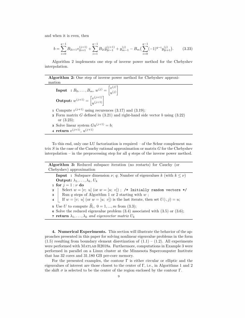
Algorithm 2 implements one step of inverse power method for the Chebyshevinterpolation.

Algorithm 2: One step of inverse power method for Chebyshev approxi-mation

Input : B0, . . . , Bm, w(j) =

[v(j)

u(j)

]Output: w(j+1) =

[v(j+1)

u(j+1)

]1 Compute v(j+1) using recurences (3.17) and (3.19);2 Form matrix G defined in (3.21) and right-hand side vector b using (3.22)

or (3.23);

3 Solve linear system Gu(j+1) = b;

4 return v(j+1), u(j+1)

To this end, only one LU factorization is required – of the Schur complement ma-trix S in the case of the Cauchy rational approximation or matrix G for the Chebyshevinterpolation – in the preprocessing step for all q steps of the inverse power method.

Algorithm 3: Reduced subspace iteration (no restarts) for Cauchy (orChebyshev) approximation

Input : Subspace dimension ν; q; Number of eigenvalues k (with k ≤ ν)Output: λ1, . . . , λk, Uk

1 for j = 1 : ν do2 Select w = [v; u] (or w = [u; v]) ; /* Initially random vectors */

3 Run q steps of Algorithm 1 or 2 starting with w ;4 If w = [v; u] (or w = [u; v]) is the last iterate, then set U(:, j) = u;

5 Use U to compute Bi, 0 = 1, ...,m from (3.3);6 Solve the reduced eigenvalue problem (3.4) associated with (3.5) or (3.6);7 return λ1, . . . , λk and eigenvector matrix Uk

4. Numerical Experiments. This section will illustrate the behavior of the ap-proaches presented in this paper for solving nonlinear eigenvalue problems in the form(1.5) resulting from boundary element disretization of (1.1) – (1.2). All experimentswere performed with Matlab R2018a. Furthermore, computations in Example 3 wereperformed in parallel on a Linux cluster at the Minnesota Supercomputer Institutethat has 32 cores and 31.180 GB per-core memory.

For the presented examples, the contour Γ is either circular or elliptic and theeigenvalues of interest are those closest to the center of Γ, i.e., in Algorithms 1 and 2the shift σ is selected to be the center of the region enclosed by the contour Γ.

9

In the case of a circular contour, the m quadrature nodes and weights used toperform the numerical integration to approximate the functions fj inside the contourΓ were generated using the Gauss-Legendre quadrature rule. To illustrate the effec-tiveness of the proposed approaches, we compare the eigenvalues obtained by eachalgorithm either with exact eigenvalues or the approximations obtained by the Beyn’smethod [5] or/and via a corresponding linearization.

Example 1. As our first example, we consider the 3D Laplace eigenvalue problem(1.1) on the unit cube Ω = [0, 1]3 with homogeneous Dirichlet boundary conditions,i.e., (1.2) with a(x) = 1 and b(x) = 0. The exact eigenvalues for this problem areknown and given by

k =√n2

1 + n22 + n2

3, ni = 0, 1, 2, . . . . (4.1)

We are interested in the six smallest eigenvalues (including multiplicities) of (1.1)presented in Table 4.1.

no. eigenvalue multiplicity1 5.441398 12 7.695299 33 9.424778 34 10.419484 35 10.882796 16 11.754763 6

Table 4.1: Approximations of the 6 smallest eigenvalues (including multiplicities)of the 3D Laplace eigenvalue problem on Ω = [0, 1]3 with homogeneous Dirichletboundary conditions [7, Table 1].

To determine these eigenvalues using the Cauchy approximation technique, wewill build the rational approximation of the matrix-valued function T (·) using circu-lar and elliptic contours. First, we compare the accuracy between the Cauchy rationalapproximation and the Chebyshev interpolation of T (·). Note that since the eigen-values of (1.1) with homogenous Dirichlet boundary condition are real we can use theChebyshev interpolation technique which target situations when the eigenvalues ofinterest lie in an interval. Figure 4.1 shows the errors of each approximation versusthe order of approximation m for both circular and elliptic contour. For simplicity, allthe errors are evaluated on a fine mesh in [−1, 1], since arbitrary curves in the complexplane can be parametrized using this interval. From this figure, we can easily see thatthe errors in the Cauchy rational approximation and Chebyshev interpolation decayexponentially with the order of the approximation m, which implies that a moderatem is usually sufficient to reach a good accuracy. To capture the eigenvalues of interest,we first consider a circle of radius r = 3.5 centered at c = 8.5. We can then solvethe linear eigenvalue problem (2.7) associated with (2.5) with m = 25 trapezoidalquadrature nodes by performing as many steps of shift-and-invert Arnoldi algorithmas needed to extract the 17 eigenvalues closest to the center c. The left hand sideof Figure 4.2 presents the eigenvalues computed by Cauchy approximation and thosecomputed by Chebyshev interpolation on a uniform mesh with 864 triangles. Note

10

that, in order to make a fair comparison between the two methods, the number of in-terpolation points for Chebyshev interpolation method is chosen to be the same as thenumber of quadrature nodes m. For Chebyshev interpolation method the real intervalenclosing the eigenvalues of interest is chosen as [5, 12]. The right hand side of Figure4.2 illustrates the comparison between the accuracy of the rational approximation andthe Chebyshev interpolation. The accuracy of an eigenpair (λ, u) is measured by therelative residual ‖T (λ)u‖2/‖u‖2. Note that the accuracy of the rational approxima-tion can be considerably improved by using an elliptic contour instead of a circle. Arational approximation (2.2) is then built using an elliptic contour centered at c = 8.5with semi-major axis rx = 3.5 and semi-minor axis ry = 0.1. The left hand side ofFigure 4.3 presents the eigenvalues computed by the Cauchy rational approximationand those computed by the Chebyshev interpolation, and the right hand side of Figure4.3 compares the relative residuals of the two methods.

We now repeat the same experiment using the Rayleigh-Ritz procedure for theCauchy and Chebyshev approximations. To extract the 17 eigenvalues listed in Table4.1, we start with a random subspace W of dimension ν = 20. We then apply q = 10steps of inverse power method to W to build a subspace of dimension ν, where eachcolumn vector is of size n. We recall that these vectors are the resulting top parts andbottom parts of the iterates of Algorithm 1 and 2 for the Cauchy and Chebyshev ap-proximations, respectively. The resulting subspace U is then orthogonalized to obtainan orthonormal basis U that can be used to perform Rayleigh-Ritz projection thatleads to a small nonlinear eigenvalue problem of size ν. This small problem is thensolved by computing the eigenvalues and eigenvectors of the expanded linear eigen-value problem (3.4) of size (m + 1)ν. The outer iterations of the reduced procedurefor the Cauchy approximation are stopped when

‖B0Xf1(Λ) +B2Xf2(Λ) + . . .+BmXfm(Λ)‖F ≤ tol,

and for the Chebyshev approximation when

‖B0Xτ1(Λ) +B2Xτ2(Λ) + . . .+BmXτm(Λ)‖F ≤ tol,

where X, Λ are the extracted eigenpairs at each iteration, ‖ · ‖F denotes the Frobe-nius norm and tol the desired tolerance for the convergence. In our experiments,we run as many outer iterations as needed to achieve convergence with a toler-ance tol = 10−12 for both Cauchy and Chebyshev approximations. This toleranceis achieved after 10 outer iterations for the Cauchy approximation and after 7 outeriterations for Chebyshev approximation. Furthermore, Figure 4.4 presents the rel-ative residuals ‖T (λ)u‖2/‖u‖2 for the 17 computed eigenvalues obtained using eachapproximation method. We ephasise that the Rayleigh-Ritz approach combined withCauchy and Chebyshev approximations delivers more accurate eigenpair approxima-tions than those computed by solving the linearized problem obtained directly fromthe Cauchy and Chebyshev approximation with projection.

Example 2. As a second example, we consider the 3D Laplace eigenvalue prob-lem (1.1) on a unit sphere with homogeneous Dirichlet boundary conditions. Theanalytic expressions for the eigenvalues for this geometry are well-known and givenas the zeros of the spherical Bessel function of order `. We are interested in the 6eigenvalues of (1.1) listed in Table 4.2.

11

100 101

m

10-20

10-15

10-10

10-5

100

App

roxi

mat

ion

erro

r

RationalChebyshev

100 101

m

10-15

10-10

10-5

100

105

App

roxi

mat

ion

erro

r

RationalChebyshev

Fig. 4.1: Left: Approximation error versus the order of the approximation m insidea unit circle. Right: Approximation error versus the order of the approximation minside an ellipse centered at c = 0 with semi-major axis rx = 1 and semi-minor axisry = 0.2.

5 6 7 8 9 10 11 12

Real part

-3

-2

-1

0

1

2

3

Imag

par

t

ContourPolesExact eigenvaluesCauchyChebyshev

100 101

Index of eigenpairs

10-20

10-15

10-10

10-5

Rel

ativ

e re

sidu

als

CauchyChebyshev

Fig. 4.2: Left: The eigenvalues of (1.1) with homogeneous Dirichlet boundary condi-tions inside a circle centered at c = 8.5 with radius r = 3.5 (circles) computed via (2.7)(plus) and Chebyshev interpolation method inside the real interval [5, 12] (squares).Right: The relative residuals ‖T (λ)u‖2/‖u‖2 of the computed eigenpairs.

no. eigenvalue multiplicity1 3.1416 12 4.4934 33 5.7634 54 6.2831 15 6.9879 76 7.7252 3

Table 4.2: Exact eigenvalues of the 3D Laplace eigenvalue problem on a unit spherewith homogeneous Dirichlet boundary conditions.

12

6 7 8 9 10 11 12

Real part

-2.5

-2

-1.5

-1

-0.5

0

0.5

1

1.5

2

2.5

Imag

par

t

ContourPolesExact eigenvaluesCauchyChebyshev

100 101

Index of eigenpairs

10-18

10-16

10-14

10-12

10-10

10-8

10-6

10-4

Rel

ativ

e re

sidu

als

CauchyChebyshev

Fig. 4.3: Left: The eigenvalues of (1.1) with homogeneous Dirichlet boundary condi-tions inside an ellipse centered at c = 8.5 with semi-major axis rx = 4.5 and semi-minor axis ry = 0.2 (circles) computed computed via (2.7) (plus) and Chebyshevinterpolation method inside the real interval [5, 12] (squares). Right: The relativeresiduals ‖T (λ)u‖2/‖u‖2 of the computed eigenpairs.

100 101

Index of eigenpairs

10-12

10-11

Rel

ativ

e re

sidu

als

100 101

Index of eigenpairs

10-18

10-17

10-16

10-15

10-14

10-13

10-12

Rel

ativ

e re

sidu

als

Fig. 4.4: Relative residuals ‖T (λ)u‖2/‖u‖2 of the 17 eigenvalues of the Laplace eigen-value problem on the unit cube. Left: after 10 outer iterations of the reduced ap-proach using Cauchy approximation. Right: after 7 outer iterations using Chebyshevapproximation.

In order to compute the eigenvalues of interest using the rational approximationtechnique, we consider an elliptic contour centered at c = 5.5 with semi-major axisrx = 2.5 and semi-minor axis ry = 0.1. The left-hand side of Figure 4.6 presentsthe eigenvalues computed by the Cauchy rational approximation and those computedby the Chebyshev interpolation with m = 25 on a uniform mesh with 384 triangles,whereas the right-hand side of Figure 4.6 illustrates the accuracy of the two methods.Also in this example, we have tested the reduced subspace iteration given by Algorithm3. To extract the 20 eigenvalues of interest, we consider the Cauchy approximationon a circle centered at c = 5.5 with radius r = 2.5. The first outer iteration wascarried out with a random subspace W of dimension ν = 25 to which q = 10 steps

13

100 101

m

10-15

10-10

10-5

100

105

App

roxi

mat

ion

erro

r

RationalChebyshev

Fig. 4.5: Approximation errors versus the order of the approximation m inside anellipse centered at c = 0 with semi-major axis rx = 1 and semi-minor axis ry = 0.2for the spherical BEM problem.

3.5 4 4.5 5 5.5 6 6.5 7 7.5 8

Real part

-1.5

-1

-0.5

0

0.5

1

1.5

Imag

par

t

ContourPolesExact eigenvaluesCauchyChebyshev

100 101

Index of eigenpairs

10-15

10-10

10-5

100

Rel

ativ

e re

sidu

als

CauchyChebyshev

Fig. 4.6: Left: The eigenvalues of (1.1) with homogeneous Dirichlet boundary con-ditions inside an ellipse centered at c = 5.5 with semi-major axis rx = 2.5 andsemi-minor axis ry = 0.2 (circles) computed via (2.7) (plus) and Chebyshev interpo-lation method inside the real interval [3, 8] (squares). Right: The relative residuals‖T (λ)u‖2/‖u‖2 associated with the computed eigenpairs.

of inverse power method, given in Algorithm 3, were applied. As for Example 1,we run as many outer iterations as needed to achieve convergence with a tolerancetol = 10−12 for both approximation methods. Note that q = 10 steps of the inversepower method were applied at each outer iteration. The Cauchy approximation andChebyshev interpolation methods achieved desired tolerance after 17 and 11 outeriterations, respectively. For completeness, we have also computed the correspondingrelative residuals ‖T (λ)u‖2/‖u‖2 for the resulting eigenpairs. These relative residualsare shown in Figure 4.7 for each eigenpair index.

Example 3. In this example, we illustrate the efficiency of the Cauchy approx-imation technique applied to the nonlinear eigenvalue problem resulting from BE

14

100 101

Index of eigenpairs

2

2.5

3

3.5

4

Rel

ativ

e re

sidu

als

10-8

100 101

Index of eigenpairs

10-15

10-14

10-13

10-12

Rel

ativ

e re

sidu

als

Fig. 4.7: Relative residuals ‖T (λ)u‖2/‖u‖2 associated with the 20 eigenvalue approx-imations of the Laplace eigenvalue problem on the unit sphere. Left: after 17 outeriterations of the reduced approach using Cauchy approximation. Right: after 11 outeriterations using Chebyshev interpolation.

discretization of a real-world problem of industrial relevance. We consider the geom-etry corresponding to a a pump casing model created by using the Gmsh tool [8].Several methods have been proposed in the literature to comprehensively study theacoustic behaviors of the pump casing [20, 17]. The boundary of the pump modeldisplayed in Figure 4.8 is partitioned into 3 479 652 triangles, leading to a nonlineareigenvalue problem with 1 728 508 DoFs. Problems of such large size add anotherlevel of difficulty to our methods, for example, we are unable to store the underlyingmatrices Bi in memory. To overcome this we resort to the H-matrix based compres-sion techniques. Specifically, we will use the Gypsilab toolbox library openHMX [2]in order to directly assemble H-matrix compressed versions of matrices Bi. Here, weconsider the boundary element discretization of problem (1.1) with a rigid boundary,i.e., b(x) = 0. For this problem, as mentioned before, complex eigenvalues may oc-cur. Hence, only the Cauchy approximation can be used to determine the eigenvaluesassociated with this problem. Since for this example the analytic expressions of theeigenvalues are not available, the relative residuals of the computed eigenpairs will beused to verify the accuracy of the obtained approximations.

Let the domain for the Cauchy approximation be given as a circular contour Ωcentered at c = −15i with radius r = 12. To choose a suitable order of approximation,we consider another circle Ω1 inside Ω with the same center and radius r1 = r/2and then increase m until the resulting rational approximation inside Ω1 is accurateenough. The eigenvalue approximations inside Ω can be obtained using a different,much coarser triangular mesh and running as many steps of Arnoldi algorithm asneeded to accurately solve the expanded linear eigenvalue problem (2.7). We recallthat only one LU factorization of the Schur complement H-matrix S is required ina preprocessing step before the actual Arnoldi algorithm is invoked. In Figure 4.9,we present the approximation errors versus the order of the Cauchy approximationon a fine mesh on Ω1. The right-hand side of Figure 4.9 shows that a high accuracyof the rational approximation can be reached for m = 24. We can therefore solvethe eigenvalue problem (1.5) using m = 24 trapezoidal quadrature nodes. Formingthe 24 matrices Bi and performing the matrix-vector multiplications with Bi are

15

Fig. 4.8: Geometry and BE mesh of the thermal model of a pump casing with 1 728 508DoFs.

efficiently parallelized on 32 cores, where the per-core memory limit is ≈ 31 GB. Theoverall computational time is 7.3 hours. The left-hand side of Figure 4.9 shows thecomputed eigenvalues. It turns out that there are 33 eigenvalues inside the contour Ω.The relative residuals ‖T (λ)u‖2/‖u‖2 associated with the computed eigenvalues arepresented in Figure 4.10 and Figure 4.11 shows 4 different modes of the pump model.

We now consider the reduced subspace iteration approach to solve the same prob-lem with 10704 triangles. To extract the same 12 eigenvalues displayed in the left-handside of Figure 4.9, we start with a random subspace W of size ν = 20 and carry out 20outer iterations of Algorithm 3 with q = 10 steps of inverse power method (Algorithm1) performed at each single outer iteration. Note that Algorithm 3 is suitable forparallelization. In our tests, we have exploited parallelism for computing the matricesBi and Bi = UTBiU using 32 cores. Since Algorithm 1 is applied to each vectorseparately to obtain a block of vectors U , the construction of the approximate sub-space at each outer iteration can also be performed in parallel. The relative residualsreached at the end of the 20 outer iterations of Algorithm 3 are displayed in Figure4.10. Figure 4.11 shows 4 modes of the model.

Acknowledgements. The authors would like to thank Mohammed Seaid for pro-viding the mesh data for the test in Example 3 of the experiments and to Gmsh teamfor making their software available. Similarly, calculations for Example 3 in the ex-periments could not have been carried out without the availability of the Gypsilabtoolbox library. The authors benefitted from the hardware resources and supportfrom the Minnesota Supercomputing Institute

REFERENCES

[1] A. Amiraslani, R. M. Corless, and P. Lancaster, Linearization of matrix polynomialsexpressed in polynomial bases, IMA J. Numer. Anal., 29 (2009), pp. 141–157.

[2] M. Aussal, The gypsilab toolbox for matlab version 0.5. openhmx library. Centre de Math-ematiques Appliquees, Ecole polytechnique, route de Saclay, 91128 Palaiseau, France.www.cmap.polytechnique.fr/~aussal/gypsilab.

16

-15 -10 -5 0 5 10 15

Real part

-25

-20

-15

-10

-5

Imag

par

t

contourpolescomp evals

101

m

10-15

10-10

10-5

100

Err

ors

Fig. 4.9: Left: The eigenvalues (inside a circle centered at c = −15i with radius r = 12)of (1.1) on the pump model domain with Robin boundary conditions computed via(2.7). Right: Approximation errors versus the order m of the Cauchy approximationinside a unit circle.

100 101

Index of eigenpairs

10-11

10-10

10-9

Rel

ativ

e re

sidu

als

Fig. 4.10: Relative residuals ‖T (λ)u‖2/‖u‖2 of the eigenvalue approximations (insidea circle centered at c = −15i with radius r = 12) of the Laplace eigenvalue problem(with Dirichlet boundary conditions) associated with the pump model displayed inFigure 4.8.

[3] M. R. Bai, Study of acoustic resonance in enclosures using eigenanalysis based on boundaryelement methods, J. Acoust. Soc. Amer., 91 (1992), pp. 25–29.

[4] M. Berljafa and S. Guttel, The RKFIT algorithm for nonlinear rational approximation,SIAM J. Sci. Comput., 39 (2017), pp. A2049–A2071.

[5] W. J. Beyn, An integral method for solving nonlinear eigenvalue problems, Linear AlgebraAppl., 436 (2012), pp. 3839–3863.

[6] R. D. Ciskowski and C. A. Brebbia, eds., Boundary Element Methods in Acoustics, SpringerNetherlands, 1991.

[7] C. Effenberger and D. Kressner, Chebyshev interpolation for nonlinear eigenvalue prob-lems, BIT, 52 (2012), pp. 933–951.

[8] C. Geuzaine and J.-F. Remacle, Gmsh: a three-dimensional finite element mesh genera-tor with built-in pre- and post-processing facilities, International Journal for NumericalMethods in Engineering, 79 (2009), pp. 1309–1331.

17

(a) Eigenfrequency: 2.87 - 5.64i Hz (b) Eigenfrequency: 3.09 - 6.22i Hz

(c) Eigenfrequency: 5.83 - 8.56i Hz (d) Eigenfrequency: -2.50 - 6.63i Hz

Fig. 4.11: Eigenmodes corresponding to four different eigenvalues

[9] S. Guttel, R. Van Beeumen, K. Meerbergen, and W. Michiels, NLEIGS: a class of fullyrational Krylov methods for nonlinear eigenvalue problems, SIAM J. Sci. Comput., 36(2014), pp. A2842–A2864.

[10] S. Guttel and F. Tisseur, The Nonlinear Eigenvalue Problem, Acta Numer., 26 (2017),pp. 1–94.

[11] F. Holstrom, Structure-acoustic analysis using BEM/FEM: Implementation in MATLAB R©,by Structural Mechanics and Engineering Acoustics, LTH, Sweden, Printed by KFS i LundAB, Lund, Sweden, (2001). http://www.akustik.lth.

[12] P. M. Juhl, The boundary element method for sound field calculations, Tech. Report 55,Technical University of Denmark, 1993. Ph.D. Thesis.

[13] P. Lietaert, J. Perez, B. Vandereycken, and K. Meerbergen, Automatic ra-tional approximation and linearization of nonlinear eigenvalue problems, Preprint.https://arxiv.org/abs/1801.08622.

[14] Y. Saad, M. El-Guide, and A. Miedlar, A rational approximation method for the nonlineareigenvalue problem, Preprint, 2019. arXiv:1901.01188.

[15] T. Sakurai and H. Sugiura, A projection method for generalized eigenvalue problems usingnumerical integration, in Proceedings of the 6th Japan-China Joint Seminar on NumericalMathematics (Tsukuba, 2002), vol. 159, 2003, pp. 119–128.

[16] S. A. Sauter and C. Schwab, Boundary element methods, vol. 39 of Springer Series in Com-putational Mathematics, Springer-Verlag, Berlin, 2011. Translated and expanded from the2004 German original.

[17] C. Tang, Y.S. Wang, J.H. Gao and H. Sugiura, Fluid-sound coupling simulation and exper-imental validation for noise characteristics of a variable displacement external gear pump,Noise Control Eng. J.), vol. 62, 2014, pp. 123–131.

[18] L.N. Trefethen and J.A.C. Weideman, The exponentially convergent trapezoidal rule, SIAMRev.), vol. 56, 2014, pp. 385–458. https://doi.org/10.1137/130932132

[19] O. Tullberg, A Study of the Boundary Element Method in Heat Conduction, Elastostaticsand Elastodynamics with Emphasis on Computer Implementation and Coupling with theFinite Element Method, Chalmers University of Technology, 1983.

[20] A. Vacca and M. Guidetti, Modeling and experimental validation of external spur gear ma-chines for fluid power applications, Simul. Model. Pract. Theory, 19 (2011), pp. 2007–2031.

[21] R. Van Beeumen, O. Marques, E. G. Ng, C. Yang, Z. Bai, L. Ge, O. Kononenko, Z. Li,C.-K. Ng, and L. Xiao, Computing resonant modes of accelerator cavities by solving non-

18

linear eigenvalue problems via rational approximation, Journal of Computational Physics,374 (2018), pp. 1031–1043.

[22] J. Xiao, C. Zhang, T.-M. Huang, and T. Sakurai, Solving large-scale nonlinear eigenvalueproblems by rational interpolation and resolvent sampling based Rayleigh-Ritz method,Internat. J. Numer. Methods Engrg., 110 (2017), pp. 776–800.

[23] C.-J. Zheng, C.-X. Bi, C. Zhang, Y.-B. Zhang, and H.-B. Chen, Fictitious eigenfrequenciesin the BEM for interior acoustic problems, Eng. Anal. Bound. Elem., 104 (2019), pp. 170–182.

19