SERIEs (2010) 1:135–169DOI 10.1007/s13209-009-0013-8

ORIGINAL ARTICLE

A rational expectations model for simulation and policyevaluation of the Spanish economy

J. E. Boscá · A. Díaz · R. Doménech · J. Ferri ·E. Pérez · L. Puch

Received: 15 May 2009 / Accepted: 22 October 2009 / Published online: 19 February 2010© The Author(s) 2010. This article is published with open access at Springerlink.com

Abstract This paper presents the model used for simulation purposes within theSpanish Ministry of Economic Affairs and Finance. REMS (a Rational ExpectationsModel for the Spanish economy) is a small open economy dynamic general equilib-rium model in the vein of the New-Neoclassical-Keynesian synthesis models, with astrongly micro-founded system of equations. In the long run REMS behaves in accor-dance with the neoclassical growth model. In the short run, it incorporates nominal,real and financial frictions. Real frictions include adjustment costs in consumption(via habits in consumption and rule-of-thumb households) and investment into phys-ical capital. Due to financial frictions, there is no perfect arbitrage between differenttypes of assets. The model also allows for slow adjustment in wages and price rigid-ities, which are specified through a Calvo-type Phillips curve. All these modellingchoices are fairly in line with other existing models for the Spanish economy. Onevaluable contribution of REMS to the renewed vintage of D(S)GE models attemptingto feature the Spanish economy is the specification of the labour market according tothe search paradigm, which is best suited to assess the impact of welfare policies onboth the intensive and extensive margins of employment. The model’s most valuableasset is the rigour of the analysis of the transmission channels linking policy actionwith economic outcomes.

J. E. Boscá · R. Doménech · J. Ferri (B)University of Valencia, Valencia, Spaine-mail: francisco.ferri@uv.es

A. Díaz · E. PérezMinistry of Economics and Finance, Madrid, Spain

R. DoménechEconomic Research Department, BBVA, Madrid, Spain

L. PuchFEDEA and ICAE, Universidad Complutense, Madrid, Spain

123

136 SERIEs (2010) 1:135–169

Keywords General equilibrium · Rigidities · Policy simulations

JEL Classification E24 · E32 · E62

1 Introduction

REMS is a small open economy dynamic general equilibrium (DGE) model thatattempts to feature the main characteristics of the Spanish economy. It builds uponthe existing literature on macroeconomic models.1 The model is primarily intendedto serve as a simulation tool within the Spanish Ministry of Economic Affairs andFinance, with a focus on the economic impact of alternative policy measures overthe medium term. REMS’ most valuable asset is the rigour of the analysis of thetransmission channels linking policy options with economic outcomes.

The small open economy assumption implies that a number of foreign variables aregiven from the perspective of the national economy and that the magnitude of spillovereffects is small. This modelling choice seems to us a fair compromise between realismand tractability.

REMS is in the tradition of DGE models. As such, it departs from MOISEES2 ina number of modelling routes. Equations in the model are explicitely derived fromintertemporal optimization by representative households and firms under technologi-cal, budgetary and institutional constraints. Thus economic decisions are solidlymicro-founded and any ad hoc dynamics has been avoided. Unlike the traditional Keynesianapproach adopted in MOISEES, with backward-looking behaviour strongly focusedon the demand side of the economy, REMS is a New Neoclassical-Keynesian synthe-sis model. Behaviour is predominantly forward-looking and short-term dynamics isembedded into a neoclassical growth model that determines economic developmentsover the long run. However, since markets do not generally work in a competitivefashion, the levels of employment and economic activity will be lower than those thatwould prevail in a competitive setting.

In the short run, REMS incorporates nominal, real and financial frictions. Realfrictions include adjustment costs in consumption (via the incorporation to the modelof habits in consumption and rule-of-thumb households) and investment into physicalcapital. Due to financial frictions, there is no perfect arbitrage between different typesof assets. The model also allows for slow adjustment in wages and price rigidities,which are specified through a Calvo-type Phillips curve. All these modelling choicesare fairly in line with other existing models for the Spanish economy. The main con-tribution of REMS to this renewed vintage of D(S)GE models is the specification

1 Many central banks and international institutions have elaborated D(S)GE models. These include, interalia, SIGMA for the US (Erceg et al. 2006), the BEQM for the UK (Harrison et al. 2005), the TOTEM forCanada (Murchison et al. 2004), AINO for Finland (Kilponen et al. 2004), or the models devised by Smetsand Wouters (2003) for EMU, Lindé et al. (2004) for Sweden and Cadiou et al. (2001) for 14 OECD coun-tries. Two models of the Spanish economy different than REMS are BEMOD and MEDEA, respectivelydeveloped by Andrés et al. (2006) and Burriel et al. (2007).2 MOISEES (Modelo de Investigacion y Simulacion de la Economia Española) is the preceding simulationtool available at the Spanish Ministry of Economic Affairs and Finance. See Molinas et al. (1990).

123

SERIEs (2010) 1:135–169 137

of the labour market according to the search paradigm. This approach has provedsuccessful in providing micro-foundations for equilibrium unemployment in the longrun and accounting for both the extensive and intensive margins of employment atbusiness-cycle frequencies. It is therefore best suited to the assessment of welfarepolicies having an impact on the labour market.

Themodel is parametrized using Spanish data. To this aim, a database (REMSDB)3

has been elaborated that satisfies the model’s estimation and calibration requirementsand serves to generate a baseline scenario for REMS.

The paper is organized as follows. Section 2 describes in detail the theoreticalmodel. Section 3 discusses the calibration strategy. Section 4 shows the properties ofthe model by analysing the basic transmission channels following standard simula-tions. The last section presents the main conclusions.

2 Theoretical framework

We model a decentralized, small open economy where households, firms, policy-makers and the external sector actively interact each period by trading one final good,government bonds, two primary production factors and one intermediate input. House-holds are the owners of the available production factors and all the firms operatingin the economy. Thus households rent physical capital and labour services out tofirms, for which they are paid interest income and wages. In the final goods sectorfirms produce goods which are imperfect substitutes for goods produced abroad. Theintermediate sector is composed of monopolistically competitive firms which produceintermediate varieties employing capital, labour and energy. Job creation is costlyin terms of time and real resources. Thus a pure economic rent arises from eachjob match over which the worker and the firm negotiate in an efficient-bargainingmanner.

Each period the government faces a budget constraint where overall expenditure isfinanced by debt issuance and various distortionary taxes. Intertemporal sustainabil-ity of fiscal balance is ensured by a conventional policy reaction function, wherebya lump-sum transfer accommodates the deviation of the debt to GDP ratio from itstarget level.

Monetary policy is managed by the European Central Bank (ECB) via a Taylorrule, which allows for some smoothness of the interest rate response to the inflationand output gap.

Each household is made of working-age agents who may be active or inactive.In turn, active workers participating in the labour market may either be employedor unemployed. Unemployed agents are actively searching for a job. Firms’ invest-ment in vacant posts is endogenously determined and so are job inflows. Finally, jobdestruction is taken as exogenous.

3 See Boscá et al. (2007), for further details.

123

138 SERIEs (2010) 1:135–169

2.1 Consumption behaviour

A large body of empirical literature documents substantial deviations of consumptionfrom the permanent-income hypothesis. To account for this evidence, we incorporateliquidity-constrained consumers into the standard Keynesian model along the linesof Galí et al. (2007). The household sector consists of a continuum of householdsof size Nt . A number N o

t of these households has unlimited access to capital mar-kets where they can buy and sell government bonds and accumulate physical capital.These financial transactions enable non-liquidity constrained households to smoothconsumption intertemporally in response to changes in the economic environment.The superscript “o” stands for “optimizing consumers”. The remaining Nr

t house-holds is liquidity constrained. These households cannot trade in financial and physicalassets and consume out of their disposable income each period. The superscript “r”stands for “rule-of-thumb (RoT ) consumers”. The size of the working-age populationis given by Nt = N o

t + Nrt . Let 1 − λr and λr denote the shares of optimizing and

RoT consumers in working age population. Working-age population, optimizing andRoT consumers all grow at the exogenous (gross) rate of γN = Nt/Nt−1, implyingthat λr is constant over time.

Let At represent the trend component of total factor productivity at time t , whichwill be assumed to grow at the exogenous rate of γA = At/At−1. Balanced growth inthe model can be ensured by transforming variables in a convenient way. More specif-ically, any flow variable Xt is made stationary through xt ≡ Xt/At−1Nt−1. Similarly,any stock variable Xt−1 is made stationary through xt−1 ≡ Xt−1/At−1Nt−1.

Following Andolfatto (1996) and Merz (1995), we assume that households pooltheir income and distribute it evenly among its members. This allows households’members to fully insure each other against fluctuations in employment.

2.1.1 Optimizing households

Ricardian households face the following maximization programme:

maxcot , no

t , jot , ko

t,bot , bo,emu

t , mot

Et

∞∑

t=0

β t[ln(co

t − hocot−1

)+ not−1φ1

(T − l1t )1−η

1 − η

+ (1 − not−1)φ2

(T − l2t )1−η

1 − η+ χm ln

(mo

t

)](1)

subject to(

rt (1 − τ kt ) + τ k

t δ)

kot−1 + wt

(1 − τ l

t

) (no

t−1l1t + rrs(1 − no

t−1

)l2t)

+((

1 − τ lt

)gst − trht

)

+ mot−1

1 + πct

+ (1 + rnt−1

) bot−1

1 + πct

+ (1 + remut−1 )

bo,emut−1

1 + πct

123

SERIEs (2010) 1:135–169 139

−(1 + τ ct )co

tPc

t

Pt− Pi

t

Ptjot

(1 + φ

2

(jot

kot−1

))− γAγN

(mo

t + bot + bo,emu

t

φbt

)= 0 (2)

γAγN kot = jo

t + (1 − δ)kot−1 (3)

γN not = (1 − σ)no

t−1 + ρwt s(1 − no

t−1) (4)

ko0, no

0, bo0, bow

0 , mo0 (5)

cot , no

t−1 and s(1− not−1) represent, consumption, the employment rate and the unem-

ployment rate of optimizing households; s is the (exogenous) share of the non-employed workers actively searching for jobs;4 T, l1t and l2t are total endowmentof time, hours worked per employee and hours devoted to job search by the unem-ployed. l1t is determined jointly by the firm and the worker as part of the same Nashbargain that is used to determine wages (see Sect. 2.4). l2t is assumed to be a functionof the overall economic activity, so that individual households take it as given.5

There are a number of preference parameters defining the utility function of opti-mizing households. Future utility is discounted at a rate of β ∈ (0, 1). The parameter ηdefines the Frisch elasticity of labour supply, which is equal to 1

η. ho > 0 indicates that

consumption is subject to habits. The subjective value imputed to leisure by workersmay vary across employment statuses, and thus φ1 �= φ2 in general.

For simplicity, we adopt the money-in-the-utility function approach to incorporatemoney into the model. The timing implicit in this specification assumes that this var-

iable is the household’s real money holdings at the end of the period (mot = Mo

tPt At N o

twhere Pt is the aggregate price level), thus after having purchased consumption goods,that yields utility.6

The maximization of (1) is constrained as follows. The budget constraint (2)describes the various sources and uses of income. The term wt (1 − τ l)no

t−1l1t

4 For simplicity, we assume that the leisure utility of the unemployed searching for a job is the same as forthe non-active:

s(1 − not−1)φ2

(T − l2t )1−η

1 − η= (1 − s)(1 − no

t−1)φ3(T − l3t )

1−η

1 − η.

5 More specifically, we assume that the search effort undertaken by unemployed workers increases duringexpansions, depending positively on the GDP growth rate:

l2t =(

l2

(gdpt

gdpt−1

)φe)(1−ρe)

lρe2t−1

where φe is the elasticity of search effort with respect to the rate of growth of GDP and ρe captures thestrength of inertia in the search effort. The reason for endogeneizing search effort in this way is an empiricalone, making possible to obtain a reasonable volatility of vacancies.6 Carlstrom and Fuerst (2001) have criticized this timing assumption on the grounds that the appropriateway to model the utility from money is to assume that money balances available before going to purchasegoods yield utility. However, we follow the standard approach in the literature whereby the end-of-periodmoney holdings yield utility.

123

140 SERIEs (2010) 1:135–169

captures net labour income earned by the fraction of employed workers, where wt

stands for hourly real wages. The product rrwt (1−τ l)s(1−not−1)l2t measures unem-

ployment benefits accruing to the unemployed, where rr denotes the replacement rateof the unemployment subsidy to the market wage. Ricardian households hold fourkinds of assets, namely private physical capital (ko

t ), domestic and euro-zone bonds(bo

t and bo,emut ) and money balances (Mo

t ). Barring money, the remaining assets yieldsome remuneration. As reflected in rt ko

t−1(1− τ k) + τ kδkot−1, optimizing households

pay capital income taxes less depreciation allowances after their earnings on physi-cal capital. Interest payments on domestic and foreign debt are respectively captured

by rnt−1

bot−1

1+πct, and remu

t−1bo,emu

t−11+πc

t, where rn and remu represent the nominal interest rates

on domestic and EMU bonds, which differ because of a risk premium (see furtherbelow). The remaining two sources of revenues are lump-sum transfers, trht , andother government transfers, gst .

The household’s consumption is given by (1+ τ c)Pc

tPt

cot , where τ c is the consump-

tion income tax. Investment into physical capital, which is affected by increasing

marginal costs of installation, is captured by Pit

Ptj ot (1 + φ

2 (jt

kt−1)). Note that the pres-

ence in the model of the relative prices Pct /Pt and Pi

t /Pt implies that a distinction ismade between the three deflators of consumption, investment and aggregate output.

The remaining constraints faced by Ricardian households concern the laws ofmotion for capital and employment. Each period the private capital stock ko

t depreci-ates at the exogenous rate δ and is accumulated through investment, jo

t . Thus, it evolvesaccording to (3). Employment obeys the law ofmotion (4), where no

t−1 and s(1−not−1)

respectively denote the share of employed and unemployed optimizing workers in theeconomy at the end of period t −1. Each period employment is destroyed at the exoge-nous rate σ and new employment opportunities come at the rate ρw

t , which representsthe probability that one unemployed worker will find a job. Although the job-findingrate ρw

t is taken as given by individual workers, it is endogenously determined at theaggregate level according to the following Cobb–Douglas matching function:7

ρwt s(1 − nt−1) = ϑt (vt , nt−1) = χ1v

χ2t[s (1 − nt−1) l2t

]1−χ2 (6)

Finally, ko0, no

0, bo0, bo,emu

0 , mo0 in (4) represent the initial conditions for all stock vari-

ables entering the maximization problem.The solution to the optimization programme above generates the following first

order conditions for consumption, employment, investment, capital stock, govern-ment debt, foreign debt and money holdings:

λo1t = 1

(Pct /Pt )(1 + τ c

t )

(1

cot − hoco

t−1− β

ho

cot+1 − hoco

t

)(7)

7 Note that this specification presumes that all workers are identical to the firm.

123

SERIEs (2010) 1:135–169 141

γN λo3t = βEt

⎧⎪⎨

⎪⎩

φ1(T −l1t+1)

1−η

1−η− φ2

(T −l2t+1)1−η

1−η

+λo1t+1wt+1

(1 − τ l

l+1

)(l1t+1 − rrsl2t+1)

+λo3t+1

[(1 − σ) − ρw

t+1

]

⎫⎪⎬

⎪⎭(8)

γAγNλo2t

λo1t

= βEtλo1t+1

λo1t

{[rt+1(1 − τ k

t+1) + τ kt+1δ

]

+φ

2

Pit+1

Pt+1

jo2t+1

ko2t

+ λo2t+1

λo1t+1

(1 − δ)

}(9)

λo2t = λo

1tPi

t

Pt

[1 + φ

(jot

kot−1

)](10)

γAγN Etλo1t

λo1t+1

= βEt1 + rn

t

1 + πct+1

(11)

γAγN λo1t

1

φbt= βEt

λo1t+1(1 + remu

t )

1 + πct+1

(12)

χm

mot

= γAγN λo1t

rnt

1 + rnt

(13)

as well as the three households’ restrictions (2), (3) and (4).Due to the presence of habits in consumption, Eq. (7) evaluates the current-value

shadow price of income in terms of the difference between the marginal utility ofconsumption in two consecutive periods t and t + 1.

Equation (8) ensures that the intertemporal reallocation of labour supply cannotimprove the life-cycle household’s utility. This optimizing rule is a distinctive featureof search models and substitutes for the conventional labour supply in the compet-itive framework. It tells us that as search is a costly process there is a premium onbeing employed, λo

3t , which measures the marginal contribution of a newly createdjob to the household’s utility. As such, λo

3t includes three terms. The first term on theright-hand side of (8) represents the difference between the value imputed to leisureby an employed and an unemployed worker. The second term captures the presentdiscounted value of the cash-flow generated by the new job in t + 1, defined as theafter-tax labour incomeminus the foregone after-tax unemployment benefits. The cur-rent-value shadow price of income, λo

1t+1, evaluates this cash-flow according to itspurchasing power in terms of consumption. The third term represents the capital valuein t + 1 of an additional employed worker corrected for the probability that the newjob will be destroyed between t and t + 1.

Expression (9) ensures that the intertemporal reallocation of capital cannot improve

the household’s utility.λo2t

λo1tdenotes the current-value shadow price of capital. This arbi-

trage condition includes two terms. The first term represents the present discountedvalue of its cash-flow in t + 1, defined as the sum of rental cost net of taxes, depre-ciation allowances and total adjustment costs evaluated in terms of consumption. Thesecond term represents the present value in t + 1 of an additional unit of productivecapital corrected for the depreciation rate.

123

142 SERIEs (2010) 1:135–169

Equation (10) states that investment is undertaken until the opportunity cost ofa marginal increase in investment in terms of consumption is equal to its marginalexpected contribution to the household’s utility.

The marginal utility of consumption evolves according to expression (11), whichis obtained by deriving the Lagrangian with respect to domestic government bondsbo

t . (11) and (7) jointly yield the Euler condition for consumption.Expression (12) is obtained by deriving the Lagrangian with respect to foreign debt

bo,emut . Note that the specification above assumes that there is no perfect arbitragebetween domestic and foreign bonds. This line is taken in Turnovsky (1985), Benigno(2001), Schmitt-Grohe and Uribe (2003) or Erceg et al. (2005), as a means to ensurethat net foreign assets are stationary. When taking a position in the international bondsmarket, optimizing households face a financial intermediation risk premium (φbt )which depends on net holdings of internationally traded bonds. The risk premium istherefore modelled as follows

ln φbt = −φb(exp(bo,emu

t)− 1

)(14)

The rest of the section simply rearrangesfirst order conditions to facilitate the economicinterpretation of Ricardian households’ behaviour. In order to obtain the arbitrage rela-tion between domestic and foreign bonds we proceed to combine (12) with (11). Thisalgebra yields

1 + rnt = φbt (1 + rnw

t ) (15)

which is the interest parity condition modified to incorporate the effect of the riskpremium. Note also that (15) differs from the standard uncovered interest parity condi-tion in that there is no risk associated with exchange rate movements, as both domesticand foreign bonds are expressed in the same currency.8

To obtain the arbitrage relation between physical capital and government bonds itis convenient to define qt ≡ λo

2t/λo1t , which allows us to rewrite Eq. (9) as

qt = 1 + πct+1

1 + rnt

[rt+1(1 − τ k

t+1) + τ kt+1δ + φ

2

j2t+1

k2t+ qt+1(1 − δ)

](16)

8 For simplicity, it is assumed that foreign bonds are expressed in euros. We could assume instead thatsome bonds could be from the rest of the world, expressed in a foreign currency. In this case, the uncoveredinterest rate parity for the euro area ensures that

1 + remut = Et

ert+1

ert(1 + rw

t )

where er is the nominal exchange rate. Given the relative small size of Spain in EMU, we assume thatthe euro exchange rate with the rest of the world is unaffected by Spanish variables, even though Spanishinflation has a small influence on ECB interest rates. This assumption is additionally supported by theempirical evidence since, as documented by many authors (see, for example, Adolfson et al. 2007, andthe references there in), the unconvered interest parity condition cannot account for the forward premiumpuzzle shown by the data. For these reasons, all foreign prices, including those of foreign bonds, are takento be exogenous and are expressed in euros.

123

SERIEs (2010) 1:135–169 143

This is a Fisher-type condition in a context characterized by adjustment costs of instal-lation of physical capital. In order to see this more clearly let φ = 0, implying that theinvestment process is not subject to any installation costs. In this case, (10) simplifiesto qt = qt+1 = 1 and expression (16) becomes

Et

[1 + (rt+1 − δ)

(1 − τ k

)]= Et

(1 + rn

t+1

1 + πct+1

)(17)

which is the conventional Fisher parity condition.Finally, expression (13) can be easily rewritten as a money demand function by

using the current-value shadow price of income (7):

mot = 1

γAγNχm(1 + τ c

t

) Pct

Pt

1 + rnt

rnt

1(1

cot −hoco

t−1− β ho

cot+1−hoco

t

) (18)

2.1.2 Rule-of-thumb households

RoT households do not have access to capital markets, so that they face the followingmaximization programme:

maxcr

t ,nrt

Et

∞∑

t=0

β t

×[ln(cr

t − hr crt−1

)+ nrt−1φ1

(T − l1t )1−η

1 − η+ (1 − nr

t−1)φ2(T − l2t )

1−η

1 − η

]

subject to the law of motion of employment (4) and the specific liquidity constraintwhereby each period’s consumption expenditure must be equal to current labourincome and government transfers, as reflected in:

wt

(1 − τ l

t

) (nr

t−1l1t + rrs(1 − nr

t−1

)l2t)

+gst

(1 − τ l

t

)− trht − (1 + τ c

t )crt

Pct

Pt= 0 (19)

γN nrt = (1 − σ)nr

t−1 + ρwt s(1 − nr

t−1) (20)

nr0 (21)

where nr0 represents the initial aggregate employment rate, which is the sole stock var-

iable in the above programme. Note that RoT consumers do not save, thus they do nothold any assets. This feature of RoT consumers considerably simplifies the solutionto the optimization programme, which is characterized by the following equations foroptimal consumption cr

t and optimal employment, nrt :

123

144 SERIEs (2010) 1:135–169

λr1t = 1

(Pct /Pt )(1 + τ c

t )

(1

crt − hr cr

t−1− β

hr

crt+1 − hr cr

t

)(22)

γN λr3t = βEt

⎧⎪⎪⎨

⎪⎪⎩

φ1(T −l1t+1)

1−η

1−η− φ2

(T −l2t )1−η

1−η

+λr1t+1wt+1

(1 − τ l

l+1

)(l1t+1 − rrsl2t+1)

+λr3t+1

[(1 − σ) − ρw

t+1

]

⎫⎪⎪⎬

⎪⎪⎭(23)

Noteworthy, the optimizing behaviour of RoT households preserves the dynamicstructure of the model, due to consumption habits and the dynamic nature of theemployment decision.

2.1.3 Aggregation

Aggregate consumption and employment can be defined as a weighted average of thecorresponding variables for each household type:

ct = (1 − λr ) cot + λr cr

t (24)

nt = (1 − λr ) not + λr nr

t (25)

For the variables that exclusively concern Ricardian households, aggregation is per-formed as:

kt = (1 − λr ) kot (26)

jt = (1 − λr ) jot (27)

bt = (1 − λr ) bot (28)

bemut = (1 − λr ) bo,emu

t (29)

mt = (1 − λr )mot (30)

2.2 Factor demands

Production in the economy takes place at two different levels. At the lower level, aninfinite number of mopolistically competing firms produce differentiated intermediategoods yi , which imperfectly substitute each other in the production of the final good.These differentiated goods are then aggregated by competitive retailers into a finaldomestic good (y) using a CES aggregator.

Intermediate producers solve a two-stage problem. In the first stage, each firm facesa cost minimization problem which results in optimal demands for production factors.When choosing optimal streams of capital, energy, employment and vacancies, inter-mediate producers set prices by varying the mark-up according to demand conditions.Variety producer i ∈ (0, 1) uses three inputs, namely, a CES composite input of private

123

SERIEs (2010) 1:135–169 145

capital and energy, labour and public capital. Technology possibilities are given by:

yit = zit

{[ak−ρ

i t−1 + (1 − a)e−ρi t

]− 1ρ

}1−α

(nit−1li1t )α(k p

it−1

)ζ(31)

where all variables are scaled by the trend component of total factor productivity and zt

represents a transitory technology shock. Each variety producer rents physical capital,kt−1, and labour services, nt−1l1t , from households, and uses public capital services,k p

t−1,provided by the government. Intermediate energy inputs et can be either importedfrom abroad or produced at home. The elasticity of substitution between private capitaland energy is given by 1

1+ρ. a ∈ (0, 1) is a distribution parameter which determines

relative factor shares in the steady state. For the sake of clarity, let us denote capitalservices by kiet as:

kiet =[ak−ρ

i t−1 + (1 − a)e−ρi t

]− 1ρ

(32)

Note that if ρ = 0 expression (32) simplifies to the Cobb–Douglas case. Our specifica-tion is more general, i.e., private capital and energy can be seen as either complements(ρ > 0) or more substitutes than Cobb–Douglas (ρ < 0), depending on the value ofρ. Our calibration strategy will nevertheless pin down the value of ρ so as to ensurethat the elasticity of substitution between private capital and energy is smaller thanthe elasticity of substitution between the capital-energy composite and labour.

Factor demands are obtained by solving the cost minimization problem faced byeach variety producer (we drop the industry index i when no confusion arises)

minkt ,nt ,vt ,et

Et

∞∑

t=0

β t λo1t+1

λo1t

(rt kt−1 + wt

(1 + τ sc) nt−1l1t + κvvt + Pe

t

Ptet(1 + τ e)

)

(33)

subject to

yt = zit

([ak−ρ

t−1 + (1 − a)e−ρt

]− 1ρ

)1−α

(nt−1l1t )α(k p

t−1

)ζ(34)

γN nt = (1 − σ)nt−1 + ρf

t vt (35)

n0 (36)

where, in accordance with the ownership structure of the economy, future profits

are discounted at the household relevant rate βλo1t+1λo1t

. κv captures recruiting costs per

vacancy, τ sc is the social security tax rate levied on gross wages, and ρf

t is the prob-ability that a vacancy will be filled in any given period t . It is worth noting that theprobability of filling a vacant post ρ f

t is exogenously taken by the firm. However, from

123

146 SERIEs (2010) 1:135–169

the perspective of the overall economy, this probability is endogenously determinedaccording to the following Cobb–Douglas matching function:

ρwt s(1 − nt−1) = ρ

ft vt = χ1v

χ2t[s (1 − nt−1) l2t

]1−χ2 (37)

Under the assumption of symmetry, the solution to the optimization programmeabove generates the following first order conditions for private capital, employment,energy and the number of vacancies

rt+1 = (1 − α)mct+1yt+1

ket+1a

(ket+1

kt

)1+ρ

(38)

γN λndt = βEt

λo1t+1

λo1t

(αmct+1

yt+1

nt− wt+1(1 + τ sc

t+1)l1t+1 + λndt+1(1 − σ)

)(39)

(1 − α)(1 − a)mctyt

ket−1

(ket

et

)1+ρ

= Pet

Pt(1 + τ e

t ) (40)

κvvt = λndt χ1v

χ2t (s(1 − nt−1)l2t )

1−χ2 (41)

where the real marginal cost (mct ) corresponds to the Lagrange multiplier associatedwith the first restriction (34), whereas λnd

t denotes the Lagrange multiplier associatedwith the second restriction (35).

The demand for private capital is determined by (38). It is positively related to themarginal productivity of capital (1−α)

yt+1ket+1

a(ket+1

kt)1+ρ times the firm’s marginal cost

mct+19 which, in equilibrium, must equate the gross return on physical capital.

The intertemporal demand for labour (39) requires the marginal contribution toprofits of a new job to be equal to the marginal product net of the wage rate plus thecapital value of the new job in t + 1, corrected for the job destruction rate between tand t + 1.

Energy demand is defined by (40). It is positively related to the marginal produc-tivity of energy (1 − α)(1 − a)

ytket−1

( ketet

)1+ρ times the marginal cost mct which, in

equilibrium, must equate the real price of energy including energy taxes.Expression (41) reflects that firms choose the number of vacancies in such a way

that the marginal recruiting cost per vacancy, κv, is equal to its expected present

value, λndt

χ1vχ2t (s(1−nt−1)l2t )

1−χ2

vt, where λnd

t denotes the shadow price of an additional

worker, and χ1vχ2t (s(1−nt−1)l2t )

1−χ2

vtis the transition probability from an unfilled to a

filled vacancy.

9 Under imperfect competition conditions, cost minimization implies that production factors are remuner-ated by the marginal revenue times their marginal productivity. In our specification for factor demands, themarginal revenue has been replaced by the corresponding marginal costs. We are legitimated to proceedin this manner because in equilibrium these two marginal concepts are made equal by the imperfectlycompetitive firm.

123

SERIEs (2010) 1:135–169 147

2.3 Pricing behaviour of intermediate firms: the New Phillips curve

Since each firm yi produces a variety of domestic goodwhich is an imperfect substitutefor the varieties produced by other firms, it acts as a monopolistic competitor facinga downward-sloping demand curve of the form:

yit = yt

(Pit

Pt

)−ε

(42)

where( PitPt

) is the relative price of variety yi , ε = (1 + ς)/ς, where ς ≥ 0 is theelasticity of substitution between intermediate goods, and yt represents the produc-tion of the final good which combines varieties of differentiated intermediate inputsas follows

yt =⎛

⎝1∫

0

y1/1+ςi t di

⎞

⎠1+ς

and Pt =⎛

⎝1∫

0

P− 1

ς

i t di

⎞

⎠−ς

(43)

Variety producers act as monopolists and set prices when allowed. As in Calvohypothesis (Calvo 1983) we assume overlapping price adjustment. Each period, aproportion θ of non-optimizing firms index prices to lagged inflation, according tothe rule Pit = (1 + πt−1)

� Pit−1 (with � representing the degree of indexation); ameasure 1 − θ of firms set their prices P̃i t optimally, i.e., to maximize the presentvalue of expected profits. Consequently, 1− θ represents the probability of adjustingprices each period, whereas θ can be interpreted as a measure of price rigidity. Thus,the maximization problem of the representative variety producer can be written as:

maxP̃i t

Et

∞∑

j=0

ρi t,t+ j (βθ) j [P̃i tπ t+ j yi t+ j − Pt+ j mcit,t+ j yi t+ j]

(44)

subject to

yit+ j = (P̃i tπ t+ j)−ε

Pεt+ j yt+ j (45)

where P̃i t is the price set by the optimizing firm at time t, β is the discount factor,mct,t+ j represents the marginal cost at t + j of the firm that last set its price in period

t , π t+ j = ∏ jh=1 (1 + πt+h−1)

� . ρt,t+ j , a price kernel which captures the marginalutility of an additional unit of profits accruing to Ricardian households at t + j , isgiven by

Etρt,t+ j

Etρt,t+ j−1= Et (λ

o1t+ j/Pt+ j )

Et (λo1t+ j−1/Pt+ j−1)

(46)

123

148 SERIEs (2010) 1:135–169

The first order condition of the optimization problem above is

P̃i t = ε

ε − 1

∑∞j=0(βθ) j Et

[ρi t,t+ j Pε+1

t+ j mcit+ j yt+ jπ−εt+ j

]

∑∞j=0(βθ) j Et

[ρi t,t+ j Pε

t+ j yt+ jπ(1−ε)t+ j

] (47)

and the corresponding aggregate price index is equal to

Pt =[θ(π�

t−1Pt−1)1−ε + (1 − θ)P̃1−ε

t

] 11−ε

(48)

As standard in the literature,10 Eq. (48) can be used to obtain an expression foraggregate inflation of the form:

πt = β

1 + �βEtπt+1 + (1 − βθ) (1 − θ)

θ(1 + �β)m̂ct + �

1 + �βπt−1 (49)

where m̂ct in mct = ε−1ε

(1+ m̂ct ) measures the deviation of the firm’s marginal costfrom the steady state. Equation (49) is known in the literature as the New PhillipsCurve. It participates of the conventional Phillips-curve philosophy that inflation isinfluenced by activity in the short run. However, the New Phillips Curve emphasizesrealmarginal costs as the relevant variable to the inflation process, which is in turn seenas a forward-looking phenomenon. This is so because when opportunities to adjustprices arrive infrequently, a firm will be concerned with future inflation. A seconddeparture of the New Phillips curve from the traditional one is that it is derived fromthe optimizing behaviour of firms. This makes it possible to define the marginal costelasticity of inflation, λ, as a function of the structural parameters in the model, β

and θ :

λ = (1 − βθ) (1 − θ)

θ(1 + �β)(50)

Equation (50) shows that an increase in the average time spell between pricechanges, θ , makes current inflation less responsive to m̂ct . Output movements willtherefore have a smaller impact on current inflation, holding expected future inflationconstant. The reduced form of the New Phillips curve can be written as:

πt = β f Etπt+1 + λm̂ct + βbπt−1 (51)

Notice that, for the sake of simplicity, the model neglects the influence of the distri-bution of prices (implicit in the Calvo hypothesis) in equilibrium. However, as shownby Burriel et al. (2007) in a DGE setting with nominal rigidities, such simplifyingassumption affects the explanatory power of the model neither dynamically nor in thesteady state.

10 See, for instance, Galí et al. (2001).

123

SERIEs (2010) 1:135–169 149

2.4 Trade in the labour market: the labour contract

The key departure of search models from the competitive paradigm is that trading inthe labour market is subject to transaction costs. Each period, the unemployed engagein search activities in order to find vacant posts spread over the economy. Costlysearch in the labour market implies that there are simultaneous flows into and outof the state of employment, thus an increase (reduction) in the stock of unemploy-ment takes place whenever job destruction (creation) predominates over job creation(destruction). Therefore unemployment stabilizes if inflows and outflows cancel outone another, i.e.,

ρf

t vt = ρwt s(1 − nt−1) = χ1v

χ2t[(1 − nt−1) l2t

]1−χ2 = (1 − σ)nt−1 (52)

Because it takes time (for households) and real resources (for firms) to make profit-able contacts, some pure economic rent emerges with each new job, which is equalto the sum of the expected search costs the firm and the worker will further incur ifthey refuse to match. The presence of such rents gives rise to a bilateral monopolyframework, whereby both parties cooperate for a win-win job match, but compete forthe share of the overall surplus.

Several wage and hours determination schemes can be applied to a bilateral monop-oly framework. In particular, we will assume that firms and workers negotiate a labourcontract in hours and wages in an efficient-bargaining manner. As discussed by Pis-sarides (2000, ch. 7, p. 176), hours of work may be determined either by the workerin such a way as to maximize his utility or by a bargain between the firm and theworker. The efficient number of hours is nevertheless determined by a Nash bargain.If workers choose their own hours of work, they will choose to work too few hours.The reason of this inefficiency is related to the existence of search costs.11

Note that, because homogeneity holds across all job-worker pairs in the economy,the outcome of this negotiation will be the same everywhere. However an individualfirm and worker are too small to influence the market. As a result when they meet theynegotiate the terms of the contract by taking as given the behaviour in the rest of themarket. The outcome of the bargaining process maximizes the weighted individualsurpluses from the match

maxwt+1,l1t+1

[λr λr

3t

λr1t

+ (1 − λr ) λo3t

λo1t

]λw (λnd

t

)(1−λw)

(53)

where λw ∈ (0, 1) reflects the worker’s bargaining power. The two terms in bracketsreflect the worker’s and firm’s surpluses from the bargain. λo

3t/λo1t and λr

3t/λr1t respec-

tively denote the earning premium of employment over unemployment for a Ricardianand a RoT worker. Similarly, λnd

t represents the profit premium of a filled over anunfilled vacancy for the representative firm. Note that this bargaining scheme featuresthe same wage for all workers, irrespective of whether they are Ricardian or RoT .

11 See also Trigari (2004) for further details about the implications of using alternatively the so calledright-to-manage hypothesis.

123

150 SERIEs (2010) 1:135–169

Efficient real wage and hours worked (53) satisfy the following conditions:

wt

(1 − τ l

)l1t = λw

[ (1 − τ l

)

(1 + τ sc)αmct

yt

nt−1+(1 − τ l

)

(1 + τ sc)

κvvt

(1 − nt−1)

]

+ (1 − λw)

[((1−λr )

λo1t

+ λr

λr1t

)(φ2

(1 − l2)1−η

1 − η− φ1

(1 − l1t )1−η

1 − η

)+(1−τ l

)gut

]

+ (1 − λw)(1 − σ − ρwt )λrβEt

λr3t+1

λr1t+1

(λo1t+1

λo1t

− λr1t+1

λr1t

)(54)

(1 − τ l

)

(1 + τ sc)αmct

yt

nt−1l1t= φ1(T − l1t )

−η

[1 − λr

λo1t

+ λr

λr1t

](55)

where we see that the equilibrium wage in a search framework is a weighted averagebetween the highest feasible wage (i.e., the marginal productivity of labour augmentedby the expected hiring cost per unemployed worker) and the lowest acceptable wage(i.e., the reservation wage, as given by the second and third terms in the right-handside of (54)).Weights are given by the parties’ bargaining power in the negotiation, λw

and (1 − λw). Notice that when λr = 0, all consumers are Ricardian, and, therefore,the solutions for the wage rate and hours simplify to the standard ones (see Andolfatto1996).

Putting aside for the moment the last term in the right-hand side of (54), the outsideoption (i.e., the reservation wage) is given, first, by the gap between the value imputedto leisure by anunemployed andby an employedworker. This gap is, in turn, aweightedaverage of the valuation of leisure by Ricardian and RoT workers, that differ in theirmarginal utilities of consumption (λo

1t and λr1t ). Notice that the higher the marginal

utility of consumption is, the higher the willingness of workers to accept relativelylower wages. Second, the reservation wage also depends on unemployment benefits(gut ). An increase in the replacement rate improves the worker’s threat point in thebargain process and exercites upward pressure to the bargained wage.

The third term in the right-hand side of (54) is a part of the reservation wage thatdepends only on the existence of RoT workers (only if λr > 0 this term is differentfrom zero). It can be interpreted as an inequality term in utility. The economic intuitionis as follows: RoT consumers are not allowed to use their wealth to smooth consump-tion over time, but they can take advantage of the fact that a matching today continueswith some probability (1−σ) in the future, yielding a labour income that, in turn, willbe used to consume tomorrow. Therefore, they use the margin that hours and wagenegotiation provides them to improve their lifetime utility, by narrowing the gap in util-ity with respect to Ricardian consumers. In this sense, they compare the intertemporal

marginal rate of substitution had not they been income constrained (λo1t+1λo1t

) with the

expected rate given their present rationing situation (λr1t+1λr1t

). For example if, caeteris

paribus,λo1t+1λo1t

>λr1t+1λr1t

the whole third term in (54) is positive, indicating that RoT

123

SERIEs (2010) 1:135–169 151

individuals put additional pressure on the average reservation wage, as a way to easetheir period by period constraint on consumption. The importance of this inequality

term is positively related to the earning premium of being matched next period (λr3t+1

λr1t+1

),

because it increases the value of a matching to continue in the future, and negativelyrelated to the job finding probability (ρw

t ), that reduces the loss of breaking up thematch.

Finally, fiscal variables also influence the division of the surplus rather than thedefinition of the worker’s and the firm’s threat points in the bargain. As commentedearlier, the replacement rate increases the bargained wage because it raises incomefrom unemployment. Both consumption and labour marginal taxes influence equilib-rium wages because the imputed value of leisure is not taxed. An increase in either τ c

tor τ l make leisure more attractive in relation to work and, by doing so, increase wagesin equilibrium. By contrast, an increase in social security contributions reduces wagesby making recruiting an additional worker more expensive.

2.5 Government

Each period the government decides the size and composition of public expenditureand the mix of taxes and new debt holdings required to finance total expenditure. Itis assumed that government purchases of goods and services (gc

t ) and public invest-ment (gi

t ) follow an exogenously given pattern, while interest payments on govern-ment bonds (1 + rt )bt−1 are model-determined, as well as unemployment benefitsgut s(1 − nt−1) and government social transfers gst which are given by

gut = rrwt (56)

gst = trgdpt (57)

whereby gut and gst are indexed to the level of real wages, wt , and activity, gdpt ,

through rr and tr .

Government revenues are made up of direct taxation on labour income (personallabour income tax, τ l

t , and social security contributions, τsct ) and capital income (τ k

t ),as well as indirect taxation, including a consumption tax at the rate τ c

t , and an energytax at the rate τ e

t . Government revenues are therefore given by

tt = (τ lt + τ sc

t )wt (nt−1l1t ) + τ kt (rt − δ) kt−1

+τ ct

Pct

Ptct + τ e

tPe

t

Ptet + trht + τ l

t rrwt s(1 − nt−1)l2t + τ lt gst (58)

where trht stands for lump-sum transfers as defined further below.Government revenues and expenditures each period are made consistent by means

of the intertemporal budget constraint

γAγN bt = gct + gi

t + gut s(1 − nt−1)l2t + gst − tt + (1 + rnt )

1 + πtbt−1 (59)

123

152 SERIEs (2010) 1:135–169

Equation (59) reflects that the gap between overall receipts and outlays is financed byvariations in lump-sum transfers to households, trht (which enter the fiscal budgetrule through the term tt ), and/or debt issuance. Note that government cannot raiseincome from seniorage.

Dynamic sustainability of public debt requires the introduction of a debt rule thatmakes one or several fiscal categories an instrument for debt stabilization. In order toenforce the government’s intertemporal budget constraint, the following fiscal policyreaction function is imposed

trht = trht−1 + ψ1

[bt

gdpt−(

b

gdp

)]+ ψ2

[bt

gdpt− bt−1

gdpt−1

](60)

where ψ1 > 0 captures the speed of adjustment from the current ratio towards the

desired target ( bgdp ). The value of ψ2 > 0 is chosen to ensure a smooth adjustment of

current debt towards its steady-state level. Note that while in the baseline specificationdebt stabilization is achieved through variations in lump-sum transfers, other receiptand spending categories could also play this role.

Government investment (exogenous in the model) augments public capital, which,given the depreciation δ p, follows the law of motion:

γAγN k pt = gi

t + (1 − δ p)k pt−1 (61)

2.6 Monetary policy

Monetary policy is managed by the ECB via the following Taylor rule, which allowsfor some smoothness of the interest rate response to the inflation and output gap

ln1 + remu

t

1 + remu=ρr ln

1 + remut−1

1 + remu+ρπ(1 − ρr ) ln

1 + πemut

1 + πemu+ρ y(1 − ρr ) ln� ln yemu

t

(62)

where all the variables with the superscript “emu” refer to EMU aggregates Thus,remu

t and πemut are the euro-zone (nominal) short-term interest rate and inflation as

measured in terms of the consumption price deflator and � ln yemut measures the rel-

ative deviation of GDP growth from its trend. There is also some inertia in nominalinterest rate setting. As discussed by Woodford (2003), (62) is the optimal outcomeof a rational central bank facing an objective function, with output and inflation asarguments, in a general equilibrium setting.

The Spanish economy contributes to EMU inflation according to its economic sizein the euro zone, ωSp:

πemut = (1 − ωSp)π

remut + ωSpπt (63)

where πremut is average inflation in the rest of the Eurozone.

123

SERIEs (2010) 1:135–169 153

The disappearance of national currencies since the inception of the monetary unionmeans that the intra-euro-area real exchange rate is given by the ratio of relative pricesbetween the domestic economy and the remaining EMU members, so real apprecia-tion/depreciation developments are driven by the inflation differential of the Spanisheconomy vis-à-vis the euro area:

rert+1

rert= 1 + πemu

t+1

1 + πt+1(64)

2.7 The external sector

The small open economy assumption implies that world prices and world demandare given from the perspective of the national economy. It also means that feedbacklinkages between the Spanish economy, EMU and the rest of the world are ignored.Another simplifying assumption concerns the nature of final and intermediate goodsproduced at home, which are all regarded as tradable.

2.7.1 The allocation of consumption and investment between domestic and foreignproduced goods

Aggregate consumption and investment are CES composite baskets of home and for-eign produced goods. Consumption and investment distributors determine the share ofaggregate consumption (investment) to be satisfied with home produced goods ch andih , and foreign imported goods c f and i f . The aggregation technology is expressedby the following CES functions:

ct =(

(1 − ωct )1σc c

σc−1σc

ht + ω1σcct(c f t) σc−1

σc

) σcσc−1

(65)

it =(

(1 − ωi t )1σi i

σi −1σi

ht + ω

1σii t

(i f t) σi −1

σi

) σiσi −1

(66)

whereσc andσi are the consumption and investment elasticities of substitution betweendomestic and foreign goods.

Each period, the representative consumption distributor chooses cht and c f t so asto minimize production costs subject to the technological constraint given by (65).The Lagrangian of this problem can be written as:

mincht ,c f t

{(Pt cht + Pm

t c f t)

+Pct

[ct −

((1 − ωc)

1σc c

σc−1σc

ht + ωc1σc(c f t) σc−1

σc

) σcσc−1]}

(67)

123

154 SERIEs (2010) 1:135–169

where Pt and Pmt are respectively the prices of home and foreign produced goods.

Note that Pct represents both the price of the consumption good for households and

the shadow cost of production faced by the aggregator.The optimal allocation of aggregate consumption between domestic and foreign

goods, cht and c f t , satisfies the following conditions:

cht = (1 − ωc)

(Pt

Pct

)−σc

ct (68)

c f t = ωc

(Pm

t

Pct

)−σc

ct (69)

Proceeding in the same manner as with the investment distributor problem, similarexpressions can be obtained regarding the optimal allocation of aggregate investmentbetween domestic and foreign goods, iht and i f t

iht = (1 − ωi )

(Pt

Pit

)−σi

it (70)

i f t = ωi

(Pm

t

Pit

)−σi

it (71)

2.7.2 Price formation

The price of domestically produced consumption and investment goods is the GDPdeflator, Pt . In order to obtain the consumption price deflator, the demands for homeand foreign consumption goods (68) and (69) need to be incorporated into the cost ofproducing one unit of aggregate consumption goods (Pt cht + Pm

t c f t ). Bearing inmindthat the unitary production cost is equal to the price of production, one can expressthe consumption and investment price deflators as a function of the GDP and importdeflators

Pct =

((1 − ωct )P1−σc

t + ωct Pm1−σct

) 11−σc (72)

Pit =

((1 − ωi t )P1−σi

t + ωi t Pm1−σit

) 11−σi (73)

The exogenous world price is a weighted average of the final and intermediate goodsprices, PFM and P

e, both expressed in terms of the domestic currency. Given the

small open economy assumption, the relevant foreign price is defined as:

Pmt =

(α̃e Pe

t + (1 − α̃e)PFMt

)(74)

where α̃e stands for the ratio of energy imports to overall imports.We assume that export prices set by Spanish firms deviate from competitors’ prices

in foreign markets, at least temporarily. This is known in the literature as the “pricing-to-market hypothesis” and it is consistent with a model of monopolistic competition

123

SERIEs (2010) 1:135–169 155

among firms where each firm regards its influence on other firms as negligible. Tomake this assumption operational, we consider a fraction of (1 − ptm) firms whoseprices at home and abroad differ. The remaining ptm goods can be freely traded byconsumers so firms set a unified price across countries (i.e., the law of one price holds).In light of the arguments above, the Spanish export price deflator is defined as

Pxt = P(1−ptm)

t(PFMt

)ptm(75)

where Pxt is the export price deflator,PFMt is the competitors’ price index expressed in

euros and the parameter ptm determines the extent towhich there is pricing-to-market.

2.7.3 Exports and imports

The national economy imports two final goods, consumption and investment, and oneintermediate commodity, energy:

imt = c f t + i f t + αeet (76)

where αe represents the ratio of energy imports over total energy consumption.Exports are a function of aggregate consumption and investment abroad, yw

t , andthe ratio of the export price deflator to the competitors price index (expressed in euros),Px

t /PFMt :

ext = sxt

(Px

t

PFMt

)−σx

ywt (77)

where σx is the long-run price elasticity of exports. Plugging (75) into (77) yields theexports demand for a small open economy under the pricing-to-market hypothesis:

ext = sxt

(PFMt

Pt

)(1−ptm)σx

ywt (78)

Note that with full pricing tomarket ptm = 0, Pxt = Pt and expression (77) simplifies

to

ext = sxt

(Pt

Pmt

)−σx

ywt = sx

t

(Pt

PFMt

)−σx

ywt (79)

Conversely, if the law of one price holds for all consumption and investment goods,then ptm = 1, Px

t = Pmt = PFMt and expression (77) simplifies to

ext = sxt yw

t (80)

123

156 SERIEs (2010) 1:135–169

Thus if the law of one price holds, exports are a sole function of total aggregateconsumption and investment from abroad. Under full pricing to market (ptm = 0),exports are also a function of relative prices with elasticity σx . Under the more generalcase of partial pricing-to-market (0 < ptm < 1), the price elasticity of exports isgiven (1 − ptm)σx .

2.7.4 Stock-flow interaction between the current account balanceand the accumulation of foreign assets

In the model, the current account balance is defined as the trade balance plus net factorincome from abroad (i.e., interest rate receipts/payments from net foreign assets):

cat = Pxt

Ptext − Pm

t

Ptimt + (remu

t − πt)

boemut−1 (81)

Following standard practice in the literature (see, for example, Obstfeld and Rogoff1995, 1996), net foreign assets are regarded as a stock variable resulting from theaccumulation of current account flows. This is illustrated by the following dynamicexpression:

γAγN boemut

φbt=(1 + remu

t

)

1 + πct

boemut−1 + Px

t

Ptext − Pm

t

Ptimt (82)

Equation (82) is obtained by combining the Ricardian households’ budget constraint(assuming a zero net supply for domestic bonds and money), the government’s budgetconstraint and the economy’s aggregate resource constraint.

2.8 Accounting identities in the economy

Gross output can be defined as the sum of (final) demand components and the (inter-mediate) consumption of energy:

yt = cht + iht + git + gc

t + Pxt

Ptext + κvvt + Pe

t

Pt(1 − αe)et + κ f (83)

where, in line with definitions above (68) and (70), cht and iht are equal to over-all domestic consumption and investment minus consumption and investment goodsimported from abroad, and κ f is an entry cost which ensures that extraordinary profitsvanish in imperfectly competitive equilibrium in the long-run. Value added generatedin the economy is given by:

gdpt = yt − Pet

Ptet − κ f − κvvt (84)

123

SERIEs (2010) 1:135–169 157

3 Model solution method and parameterization

3.1 Model solution method

The number of equations involved in the model and the presence of non-linearities donot allow for a closed-form solution for the dynamic stable path. In order to providea solution for dynamic systems of this nature it has become a common procedure inthe literature to use a numerical method. There are several ways of solving forward-looking models with rational expectations. Most of them rely on algorithms that areapplied to the linearized version of the system around the steady state. This approach,which is very popular in the literature, was first introduced by Blanchard and Kahn(1980).

In order to solve the model we follow the method developed by Laffarque (1990),Boucekkine (1995) and Juillard (1996). As various endogenous variables in the modelhave leads, representing expectations of these variables in future time periods, anassumption has to be made regarding the formation of expectations. In REMS expec-tations are rational and, therefore, model-consistent. This means that each period’sfuture expectations coincide with the model’s solution for the future. In simulationsthis implies that the leads in the model equations are equal to the solution valuesfor future periods. This rational expectations solution is implemented by applying astacked-time algorithm that solves for multiple time periods simultaneously, i.e., itstacks the time periods into one large system of equations and solves them simulta-neously using Newton–Raphson iterations. The method is robust because the numberof iterations is scarcely affected by convergence criteria, the number of time periodsor the size of the shock. The model is simulated using the Dynare software system.

REMS obeys the necessary local condition for the uniqueness of a stable equilib-rium in the neighbourhood of the steady state, i.e., there are asmany eigenvalues largerthan one in modulus as there are forward-looking variables in the system.

3.2 The database REMSDB

The database REMSDB includes the main Spanish economic aggregates (see Boscáet al. 2007, for further details). The complete set of series covers the period 1980–2010,which in turn can be divided into two sub-periods depending on the nature of the data.The first one ranges from 1980 to the last available data released by the various statis-tical sources, i.e., 2007 in the current version of the database. The second one, whichspans over a 5-year period, relies on the official forecasts reflected in the Stability andGrowth Programme (SGP). In the existing version of REMSDB the last available yearof the forecast period corresponds to 2010. Finally, in order to generate a baselinescenario for the REMS model, the whole set of variables are extended forward until2050. Such data extrapolation complies with the balanced-growth hypothesis of themodel.

All series are quarterly data. In most cases, data on a quarterly basis were readilyavailable from the existing statistical sources. Annual series were transformed intoquarterly by applying the Kalman filter and smoother to an appropriate state-space

123

158 SERIEs (2010) 1:135–169

model in which observations correspond to low-frequency data. Monthly series wereconverted into quarterly data with techniques that are specific to each series. All seriestake the form of seasonally adjusted data.Whenever the series provided by official sta-tistical sources were not so, they were seasonally adjusted through TRAMO-SEATSprocedures.

The data compiled in REMSDB has generally not been subject to any transforma-tion other than the extraction of the seasonal component or the mere application oflinking-back techniques. The group of variables used to construct the baseline scenariohave nevertheless been expressed in efficiency units in order to ensure the stationaryproperty.

The database considers five types of variables. While each of these groups is some-what stylized, they gather a set of variables of a different nature. The first categoryincludes production and demand aggregates and their deflators. A second group bringstogether population and labour-market series. The third block is made up of mone-tary and financial variables, whereas the fourth one includes aggregates of the generalgovernment. A final group gathers a number of heterogeneous variables used in thebaseline scenario and for which no direct statistical counterpart is available from offi-cial sources.

3.3 Model parameterization

Model parameters have been fixed using a hybrid approach of calibration and estima-tion. Some parameter values are taken from QUEST II and other related DGEmodels.Several other parameters are obtained from steady-state conditions. The remainingparameters have been estimated on the basis of selected model’s equations. Alto-gether, these parameters produce a baseline solution that accurately resembles thebehaviour of the Spanish economy over the last two decades.

The data used for calibration purposes come from the REMSDB database and coverthe period 1985:3 2006:4, during which the behaviour of endogenous variables com-plies with cyclical empirical regularities (see Puch and Licandro 1997; Boscá et al.2007). The group of variables without statistical counterpart in official sources includeconsumption and employment of RoT and optimizing consumers, the Lagrangemulti-pliers, theTobin’sq, the composite of private physical capital and energy,marginal costand total factor productivity. These variables are computed using their correspondingbehavioural equations in the model.

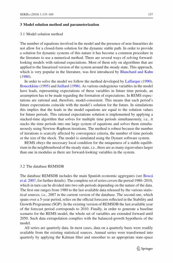
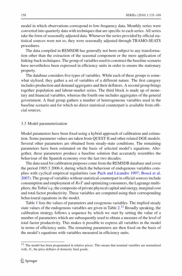
Table 1 lists the values of parameters and exogenous variables. The implied steadystate values of the endogenous variables are given in Table 2.12 Broadly speaking, thecalibration strategy follows a sequence by which we start by setting the value of anumber of parameters which are subsequently used to obtain a measure of the level oftotal factor productivity. This makes it possible to express all variables in the modelin terms of efficiency units. The remaining parameters are then fixed on the basis ofthe model’s equations with variables measured in efficiency units.

12 The model has been programmed in relative prices. This means that nominal variables are normalizedwith, Pt , the price deflator of domestic final goods.

123

SERIEs (2010) 1:135–169 159

Table 1 Parameter values

θ 0.5400 γ 1.75 κ f 0.129148 ρw 0.75

α 0.59387 ρr 0.75 PFM 1.002991 φe 25

ζ 0.06(

bgdp

)2.40 yw 7.306437 ρe 0.85

δ 0.01587 rr 0.20225 T 1.369 s 0.269341

δ p 0.01058 τ l 0.110766 χm 0.20347 φb 0.006

κv 0.18414 τ k 0.208272 sx 0.021345 ptm 0.57675

σ 0.08625 τ c 0.106985 ωc 0.1395 λw 0.42743

χ1 0.61158 τ sc 0.221531 ωi 0.423765 mc 0.840691

χ2 0.57257 τ e 0.20 λr 0.5 σc 1.20548

l2 0.21828 ψ1 0.01 ho 0.6 σx 1.3

φ1 3.23775 ψ2 0.2 hr 0.0 σi 0.93043

φ2 2.59905 η 2.0 αe 0.498 λ 0.2006

ρ 0.99776 γA 1.00170 α̃e 0.10489 β f 0.4965

a 0.99888 γN 1.00325 tr 0.138154 βb 0.5035

φ 5.50 rnw 0.0142 trh 0.0259859 ωSp 0.1000

Table 2 Steady state

bt 1.4207 iht 0.0787 λr3t 1.5633 gst 0.0818

bot 1.4207 imt 0.1542 λnd

t 0.5119 trht 0.0326

ct 0.3618 jt 0.1408 λo1t 2.2221 tt 0.2104

c f t 0.0633 jot 0.2816 λr

1t 3.1218 gut 0.2724

cht 0.2999 ρwt 0.0732

pct

pt0.9694 vt 0.1120

cot 0.4251 kt 6.7604 πt 0.0000 wt 1.5147

crt 0.2985 ket 5.7032 gdpt 0.5920 w̃t 1.5147

et 0.0402 kot 13.521 πc

t 0.0000 yt 0.7764

rer t 0.8157 k pt 1.1028

pit

pt0.9119 zt 1.0000

ext 0.1394 mt 3.2536pm

tpt

0.8037 git 0.0171

bwt 0.0000 m̂ct 0.0000

pxt

pt0.8892

bowt 0.0000 mo

t 6.5072 qt 1.0164

gct 0.0895 nt 0.4499 rt 0.0331

l1t 0.4369 not 0.4499 rn

t 0.0142

it 0.1489 nrt 0.4499 φbt 1.0000

i f t 0.0709 λo3t 0.1560 l2t 0.2183

The Cobb–Douglas parameter α matches the average value of the labour share inthe data, as measured by the ratio of compensation of employees to GDP. The publiccapital elasticity of output, ζ , has been set at 0.06, which falls within the range ofthe estimated values reported by Gramlich (1994). Given the values of α and ζ it isstraightforward to obtain the level of technological efficiency, At , using expression

123

160 SERIEs (2010) 1:135–169

(31). HP-filtered total factor productivity is then used to rescale all variables withrespect to efficiency. Technical progress, γA, is given by the growth rate of trendproductivity.

The calibrated values of a number of parameters are taken from QUEST II. Thisis the case of the subjective discount rate, β, the parameter of adjustment costs inthe investment function, φ, the long-run price elasticity of exports, σx , and fiscal ruleparameters, ψ1 and ψ2.

Following Andolfatto (1996), we choose a value of 2 for parameter defining thedegree of intertemporal labour substitution, η, whereas the amount of time devoted tolooking for a job, l2, is estimated as half as much the quarterly average of workingtime. κv is calibrated to match an overall cost of vacant posts equal to 0.5% points ofGDP. As in Burnside et al. (1993) we fix total productive time endowment T at 1.369(thousand) hours per quarter. The exogenous job destruction rate, σ , is calibrated fromthe law of motion of the employment (4). The share of non-employed workers activelysearching for a job, s, is obtained from the ratio between the unemployment rate andone minus the employment rate, (1 − n).

We follow Doménech et al. (2002) in calibrating the parameters that enter the mon-etary policy reaction function γE MU and ρr

EMU. The weight of the Spanish economyin the euro-zone inflation, ωSp, is set at 10%. The public debt to GDP target ratiohas been set at 2.4. This corresponds to a 60% value on an annual basis, which isequal to the limit established in the Stability and Growth Pact. Tax rates on labour andcapital income and consumption expenditure (τ l , τ k , τ sc, τ c) have been constructedfollowing the methodology developed by Boscá et al. (2005). Tax rate on energy, τ e

t ,has been set at 0.20. The growth rate of population, γN , has been computed on thebasis of working-age population data. We use the ratio of unemployment benefits tolabour compensation to calibrate the replacement rate, rr .

The value of 0.6 for ho, the parameter that captures habits in consumption of Ri-cardian households, has been taken from Smets and Wouters (2003). The fraction ofRoT consumers in the Spanish economy, λr , is assumed to be 0.5 which is a quitestandard value. The risk premium parameter, φb, is fixed at 0.006. This is somewhathigher than the value in Erceg et al. (2005), implying faster convergence of the foreignasset position to the steady state. The scale parameter of the matching function, χ1,and the elasticity of matchings with respect to vacant posts, χ2, have been estimatedat, respectively, 0.61 and 0.57, respectively. In line with the efficiency condition inHosios (1990), the workers’ bargaining power is set at 1 − χ2.

The entry cost, κ f , is calculated at 0.13 from a markup of 20%. Using data onthe weight of intermediate inputs in gross output from the Input-Output tables, thedistributional parameter in the energy-capital composite, a, has been set to 0.99.Theestimated value ofρ is 0.99,which corresponds to an elasticity of substitution 1/(1+ρ)

of 0.50, implying that private capital and energy are complements in production. Valueadded is then computed using the accounting identity (84). The ratio of energy importsto total energy consumption, αe, is taken from the Input-Output Tables (year 2000).Private and public capital depreciation δ and δ p are the rates implicit in the capitalseries in BDREMS, respectively around 6 and 4% per year.

As regards preference parameters in the households utility function, φ1 and φ2,

the former is estimated from the hours schedule Eq. (55), whereas the latter has been

123

SERIEs (2010) 1:135–169 161

computed as a weighted average (with weights λr and (1− λr )) of the estimates aris-ing from the two labour supply conditions, (8) and (23). Overall, our values for φ1and φ2 resemble those obtained by Andolfatto (1996) and other related research inthe literature, implying that the imputed value for leisure by an employed worker issituated well above the imputed value for leisure by an unemployed worker.

We use the employment demand (39) to obtain a series for the firm’s marginal cost,mct . The steady state value, mc, is set at the sample mean. We choose the degree ofprice indexation � at 1 (hypothesis testing of an estimated value of 1 for � resultsin no rejection), and use expression (49) to obtain a GMM estimation of the fractionof non-optimizing firms, θ . The estimated value is equal to 0.54. Together with thesubjective discount rate, these two parameters imply a value of 0.20 for the marginalcost elasticity of inflation, λ,13 and 0.50 for the weights attached to the forward andbackward components of inflation, β f and βb. Values of these parameters about onehalf are a key feature of the hybrid Phillips curve with full indexation, as evidencedby the empirical literature.14

In the external sector, we have used Eqs. (75) and (74) to obtain estimations of thepricing-to-market parameter, ptm, and the ratio of energy imports to overall imports,α̃e. Our estimate for α̃e suggests that energy represents around 10% of total imports.The estimated value of ptm parameter (0.58) is of the same order of magnitude as inQUEST II (0.61). The weight of domestic consumption goods in the CES aggrega-tor, ωc, and the consumption elasticity of substitution between domestic and foreigngoods, σc, are estimated simultaneously using conditions (68) and (69). Similarly, forthe case of investment goods, ωi and σi are estimated simultaneously using Eqs. (70)and (71). The estimated elasticities suggest a slightly higher elasticity of substitu-tion between domestic and foreign goods for consumption goods as compared withinvestment goods. We use the export equation (77) to calibrate the scale parameter sx .The energy price index, Pe, and the world price index, PFM, match sample averagescalculated over the calibration period.

The value of two parameters has been accommodated to ensure the desirable long-run properties of the model. The world interest rate, remu , is set to satisfy the staticversion of Eq. (11), so that the current account is balanced in the steady state. Second,foreign output, yw, is adjusted to obtain a steady state value of the real exchange rateclose to the observed one.

Finally, the value of a number of parameters has been chosen for labour marketvariables to display plausible dynamic patterns. Namely, we assume partial inertia inthe search effort, ρe. As in Blanchard and Galí (2006), we allow for slow adjustment inwages, which evolve according to the expression wt = w

ρw

t−1w̃(1−ρw)t , with w̃t being

the Nash-bargained wage. This hypothesis is introduced in the model in an ad hocmanner, with an estimated value of ρw = 0.75.

13 This value is significantly higher than that obtained by Galí and Lopez-Salido (2001).14 Bils and Klenow (2004) find that the average duration between price adjustments is over six months.The evidence on price setting in the euro area at the individual level by Álvarez et al. (2006) shows thatprices in the euro area are stickier than in the US.

123

162 SERIEs (2010) 1:135–169

0 10 20 30 40-0.5

0

0.5

1

1.5GDP

0 10 20 30 40-1

-0.5

0

0.5

1

1.5Private consumption

0 10 20 30 40-1

0

1

2

3

4Investment

0 10 20 30 40-0.2

-0.1

0

0.1

0.2Trade surplus/GDP

0 10 20 30 40-1

-0.5

0

0.5

1

1.5Employment

0 10 20 30 40-0.2

0

0.2

0.4

0.6Real wage

0 10 20 30 40-0.8

-0.6

-0.4

-0.2

0

0.2GDP deflator inflation

0 10 20 30 40-1

-0.5

0

0.5Hours

0 10 20 30 40-2

0

2

4

6

8Vacancies

Total

Ricardian

RoT

Fig. 1 Effects of a transitory technological shock

4 Simulations

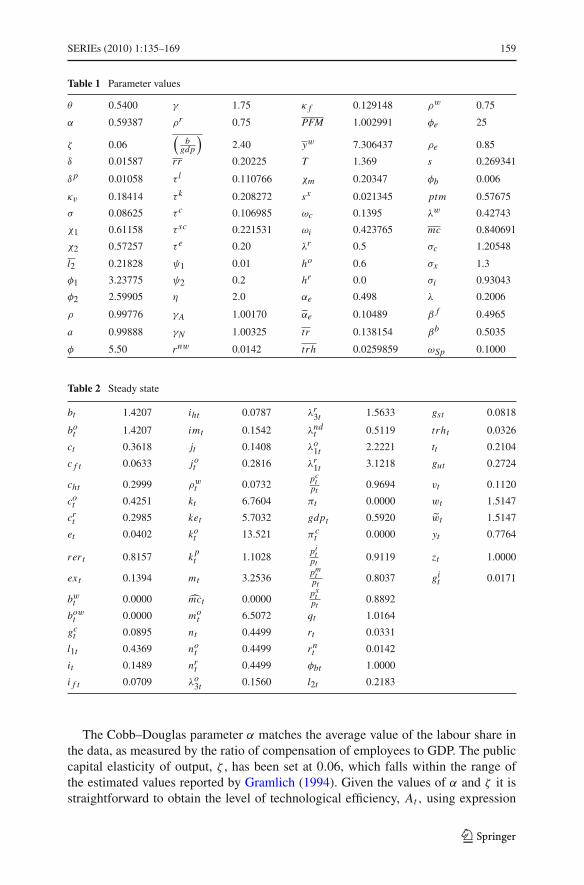
This section shows the properties of the model and examines the basic transmissionchannels at work by presenting some simulation exercises. First, we show results oftwo standard simulated scenarios, a technology shock and a public consumption shock.The two shocks are of a temporary nature and fully anticipated by economic agents.Finally, we end this section with the simulated short and long-run impacts on somemacroeconomic variables of a menu of fiscal policies.

4.1 A transitory technology shock

In this section an exogenous productivity improvement is implemented as a 1%increase of zi . The technology shock ismodelled as a first-order autoregressive processwith a persistence parameter of 0.9, implying that the level of total factor productivityafter 5years is situated 0.2% points above the steady state level.

Figure 1 displays the (quarterly) dynamic responses of selected macroeconomicvariables in the model. Simulation results are percentage deviations from baseline,except for the trade surplus and the GDP deflator inflation, which are absolute devia-tions.

123

SERIEs (2010) 1:135–169 163

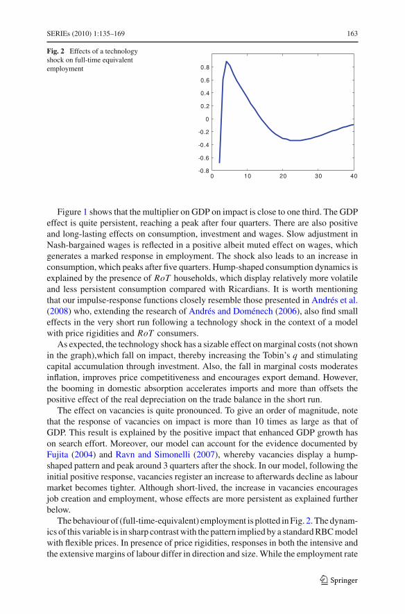
Fig. 2 Effects of a technologyshock on full-time equivalentemployment

0 10 20 30 40-0.8

-0.6

-0.4

-0.2

0

0.2

0.4

0.6

0.8

Figure 1 shows that the multiplier on GDP on impact is close to one third. The GDPeffect is quite persistent, reaching a peak after four quarters. There are also positiveand long-lasting effects on consumption, investment and wages. Slow adjustment inNash-bargained wages is reflected in a positive albeit muted effect on wages, whichgenerates a marked response in employment. The shock also leads to an increase inconsumption, which peaks after five quarters. Hump-shaped consumption dynamics isexplained by the presence of RoT households, which display relatively more volatileand less persistent consumption compared with Ricardians. It is worth mentioningthat our impulse-response functions closely resemble those presented in Andrés et al.(2008) who, extending the research of Andrés and Doménech (2006), also find smalleffects in the very short run following a technology shock in the context of a modelwith price rigidities and RoT consumers.

As expected, the technology shock has a sizable effect onmarginal costs (not shownin the graph),which fall on impact, thereby increasing the Tobin’s q and stimulatingcapital accumulation through investment. Also, the fall in marginal costs moderatesinflation, improves price competitiveness and encourages export demand. However,the booming in domestic absorption accelerates imports and more than offsets thepositive effect of the real depreciation on the trade balance in the short run.

The effect on vacancies is quite pronounced. To give an order of magnitude, notethat the response of vacancies on impact is more than 10 times as large as that ofGDP. This result is explained by the positive impact that enhanced GDP growth hason search effort. Moreover, our model can account for the evidence documented byFujita (2004) and Ravn and Simonelli (2007), whereby vacancies display a hump-shaped pattern and peak around 3 quarters after the shock. In our model, following theinitial positive response, vacancies register an increase to afterwards decline as labourmarket becomes tighter. Although short-lived, the increase in vacancies encouragesjob creation and employment, whose effects are more persistent as explained furtherbelow.

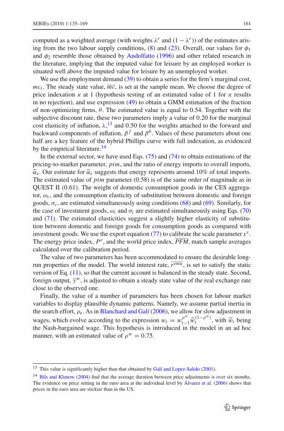
Thebehaviour of (full-time-equivalent) employment is plotted inFig. 2.Thedynam-ics of this variable is in sharp contrastwith the pattern implied by a standardRBCmodelwith flexible prices. In presence of price rigidities, responses in both the intensive andthe extensive margins of labour differ in direction and size.While the employment rate

123

164 SERIEs (2010) 1:135–169

0 10 20 30 40-0.5

0

0.5

1GDP

0 10 20 30 40-1

0

1

2Private consumption

Total

Ricardian

RoT

0 10 20 30 40-1.5

-1

-0.5

0Investment

0 10 20 30 40-0.15

-0.1

-0.05

0

0.05Trade surplus/GDP

0 10 20 30 40-0.1

0

0.1

0.2

0.3Employment

0 10 20 30 40-0.3

-0.2

-0.1

0

0.1Real wage

0 10 20 30 40-0.2

0

0.2

0.4

0.6GDP deflator inflation

0 10 20 30 400

0.5

1

1.5Hours

0 10 20 30 40-2

-1

0

1

2

3Vacancies

Fig. 3 Effects of a transitory public consumption shock

rises over time, hours per worker sharply falls on impact. Overall, (full-time equiva-lent) employment falls over the first four quarters, and only attains pre-shock levelsafter 1year. These predictions match the empirical findings of a growing literaturebeginning with Galí (1999) (see, for instance, Section 2 in Galí and Rabanal 2004 andAndrés et al. 2008, for an overview of research studies with similar conclusions).

4.2 A transitory public consumption shock

With a view to illustrate further transmission channels in REMS, this section discussesan exogenous transitory shock affecting the steady-state level of public consumption.The fiscal impulse amounts to 1% of baseline GDP (or 6.5% of gc) and it is assumedto follow a first-order autoregressive process with a persistence parameter of 0.9.Figure 3 displays the quarterly dynamic responses of the main macroeconomic vari-ables in the model.

The multiplier on GDP (�GDP/�gc) on impact is equal to 1. A transitory impulseto public consumption leads to a significant increase in consumption (by around 0.5%points on impact), that lasts for about two quarters. This is confirmed by existing evi-dence of models allowing for liquidity-constrained (see Blanchard andGalí 2006; Galíet al. 2007). As suggested by the second panel in Fig. 3, the dynamics of overall con-sumption is largely driven by the behaviour of RoT households, whose consumption

123

SERIEs (2010) 1:135–169 165

Fig. 4 Effects of a publicconsumption shock on full-timeequivalent employment

0 10 20 30 400

0.2

0.4

0.6

0.8

1

1.2

1.4

1.6

increases on impact by more than 1% point. In contrast, optimizing households, whichare fully aware of the transitory nature of the shock, revise their current consumptiondownwards to offset the negative effect of the fiscal stimulus on government savings.

Private investment falls immediately after the shock and continues dropping up to1.5% after three to four quarters, suggesting a sizable crowding-out effect. The troughin investment can be rationalized in terms of a decline in Tobin’s q, a slightly highereuro-zone nominal interest rate (as higher inflation and output gaps in the Spanisheconomy affect the corresponding euro-zone variables in a proportion determined bythe weight of the domestic economy in the euro area), and a higher risk premium. Thelatter results in a lower level of external debt hold by domestic households.

Figure 3 shows that employment, hours, real wages and vacancies increase onimpact, then gradually return to normal. The jump in vacant posts is explained byimproved search effort and a higher shadow price of employment, λnd . Full-timeequivalent employment (see Fig. 4) is enhanced by the positive response of employ-ment both in terms of headcounts and hours worked.

4.3 Choosing among different fiscal policies

We use now REMS to simulate the short (Table 3) and long run effects (Table 4) ofperforming different fiscal policy measures. In all cases we show the impact on GDP,employment and the ratio of public debt to GDP. Thus, we analyse the effects of a 1%point reduction in the effective labour tax rate (row 1), of a 1% point reduction in theeffective consumption tax rate (row 2), of a 1% GDP increase in public consumption(row 3) and of a 1% GDP increase in public investment (row 4). Finally, in row 5 wetake into account the proposal of Fernández-Villaverde and Rubio-Ramírez (2009)simulating the effects of a 2% point reduction in the labour tax rate, together with a1% point increase in the consumption tax rate. According to their results a 1% pointreduction in the effective labour tax rate in Spain would increase GDP on impact by1.076%, whereas a 1% point reduction in the effective consumption tax rate wouldcause a rise in GDP of 0.175%. Both measures taken together, which constitute theirpreferred policy-mix, would increase GDP by about 2% on impact. Surprisingly their

123

166 SERIEs (2010) 1:135–169

Table 3 Fiscal policies (1year multiplier)

Economic policy measure GDP Employment Public debt/GDP

(1) Labour tax reduction (1%) 0.353 0.620 0.285

(2) Consumption tax reduction (1%) 0.285 0.501 0.269

(3) Public consumption increase (1% of GDP) 0.336 0.621 0.137

(4) Public investment increase (1% of GDP) 0.677 0.927 −0.077

(5) Fernández-Villaverde & Rubio proposal 0.421 0.737 0.302

Table 4 Fiscal policies (long run multiplier)

Measure GDP Employment Public debt/GDP

(1) Labour tax reduction (1%) 0.54 0.59 0

(2) Consumption tax reduction (1%) 0.44 0.48 0

(3) Public consumption increase (1% of GDP) 0.94 0.85 0

(4) Public investment increase (1% of GDP) 3.28 0.23 0

(5) Fernández-Villaverde & Rubio proposal 0.64 0.69 0

results show that increasing public investment 1% point would reduce GDP on impacta 1.124%.

Our results are in contrast with those of Fernández-Villaverde and Rubio-Ramírez(2009). Looking at the 1year multipliers in Table 3 (calculated as a simple aver-age of simulated effects in the first four quarters), we find that public investmentwould generate the biggest effect both on GDP, that would increase a 0.677%, andon employment, that would rise by almost 1% point. The Fernández-Villaverde andRubio-Ramírez (2009) proposal is the second preferred option in the ranking of simu-lations performed with REMS, although with lower impact that the one calculated bythese authors. Moreover, the cost of this proposal in terms of public debt is the highestone among all fiscal policy actions considered. In the long run, when the public debtto GDP ratio returns to its initial value, the primacy of public investment policieswith respect to other ways of implementing fiscal policies is even more pronounced.Thus, our simulations give support to the recent government injection of 8,000 millioneuros to finance public investment (Plan E), when comparing its effects on GDP andemployment with other fiscal measures based on transfers to households or tax cuts.

5 Conclusions

This paper presents a Rational Expectations Model for Simulation and Policy Eval-uation of the Spanish Economy (REMS). REMS is a DGE model for a small openeconomy. It is primarily constructed to serve as a tool for simulation and policy eval-uation of alternative scenarios. This means that REMS is not used for forecasting, butrather to analyse how the effects of policy shocks are transmitted over the medium

123

SERIEs (2010) 1:135–169 167

term. It also means that the emphasis of the model is on the transmission channelsthrough which policy action affects the domestic economy.

As far as economic theory is concerned, REMS can be characterized as a NewKeynesian model with the optimizing behaviour of households and firms being deeplyrooted in the Rational Expectations hypothesis. The supply side of the economy ismodelled through a neoclassical production function, implying that the long-termbehaviour of the model closely reproduces the Solow growth model, that is, the econ-omy reaches a steady state path with a growth rate determined by the rate of exogenoustechnical progress plus the growth rate of the population. However, some prominentfeatures differentiate this model from the neoclassical paradigm in the long term.First, trading both in the goods and the labour market is not achieved under Walrasianconditions. Firms in goods markets operate under monopolistic competition, settingprices in a sluggish manner. In the labour market, firms and workers negotiate howto distribute the rents generated in the matching process. Consequently, in our modelequilibrium unemployment will persist in the long term. Second, a share of householdsbehaves as myopic consumers that do not optimize intertemporally. Additionally, con-sumers take into account past consumption (habits) in their decisions. As a result, thebehaviour of aggregate consumption after a fiscal shock departs considerably fromwhat could be expected in a neoclassical setting. In the short term REMS is also influ-enced by the New Keynesian literature allowing for a stabilizing role of demand-sidepolicies.

Nevertheless, the model still lacks sufficient detail to make a direct link betweensome specific reform efforts and economic performance. Several ways of improvingthe model are opened for the future. For instance, a weak point of the existing ver-sion of the model is that it is not detailed enough to differentiate across skill groupsof the labour force. Also, REMS sticks on the exogenous nature of technical pro-gress, whereas it is widely recognized by now that knowledge investment is a keyto economic growth and there is a link between the growth rate of technical pro-gress and R&D spending. Moreover, as the recent financial crisis has made it cleara better understanding is needed of the linkages between the financial sector andthe real sector. A final improvement of the model concerns estimation techniques.Forthcoming versions of REMS should estimate the model using Bayesian estimationtechniques.

Acknowledgments This research could have not been accomplished without the unconditional supportof Juan Varela. We would like to thank the helpful comments and suggestions of Javier Andrés, PabloBurriel, Francisco Corrales, Ángel de la Fuente, Víctor Gómez, Luis González-Calbet, Campbel Leith,Ángel Melguizo, Eduardo Pedreira, Álvaro Sanmartín and participants at the workshop on Lisbon method-ology organized by the EU Commission and at the XXXII SAE. The work of Andrés de Bustos with thedataset has been invaluable. Financial support from the European Regional Development Fund (ERDF) andFundaciónRafael del Pino is gratefully acknowledged. J. E.Boscá and J. Ferri also thank thefinancial supportby CICYT Grants ECO2008-04669 and ECO2009-09569 and Luis Puch CICYT Grant SEJ2004-04579.

Open Access This article is distributed under the terms of the Creative Commons Attribution Noncom-mercial License which permits any noncommercial use, distribution, and reproduction in any medium,provided the original author(s) and source are credited.

123

168 SERIEs (2010) 1:135–169

References

Adolfson M, Laséen S, Lindé J, Villani M (2007) Evaluating an estimated new Keynesian small openeconomy model. Working Paper Series 203. Sveriges Riksbank

Álvarez L, Dhyne E, Hoeberichts M, Kwapil C, Le Bihan H, Lünnemann P, Martins F, Sabbatini R, StahlH, Vermeulen P, Vilmunen J (2006) Sticky prices in the Euro area: a summary of new microevidence.J Eur Econ Assoc 4(2–3):575–584

Andolfatto D (1996) Business cycles and labor-market search. Am Econ Rev 86(1):112–132Andrés J, Burriel P, Estrada A (2006) BEMOD: a DSGE model for the Spanish economy and the rest of

the Euro area. Banco de España Research Paper, No. WP-0631Andrés J, Doménech R (2006) Automatic stabilizers, fiscal rules and macroeconomic stability. Eur Econ

Rev 50(6):1487–1506Andrés J, Doménech R, Fatás A (2008) The stabilizing role of government size. J Econ Dyn Control

32:571–593Benigno P (2001) Price stability with imperfect financial integration. CEPR Discussion Paper No. 2854Bils M, Klenow P (2004) Some evidence on the importance of sticky prices. J Political Econ 112(5):947–

985Blanchard OJ, Galí J (2006) A new Keynesian model with unemployment. MIT Department of Economics

Working Paper No. 06-22Blanchard OJ, Kahn CM (1980) The solution of linear difference models under rational expectations. Eco-

nometrica 48:1305–1311Boscá JE, García JR, Taguas D (2005) Tipos Efectivos de Gravamen y Convergencia Fiscal en la OCDE:

1965–2001. Hacienda Pública Española 174(3):119–141Boscá JE, Bustos A, Díaz A, Doménech R, Ferri J, Pérez E, Puch L (2007) The REMSDB macroeconomic

database of the Spanish economy. Working Paper WP-2007-04. Ministerio de Econom ía y HaciendaBoucekkine R (1995) An alternative methodology for solving non linear forward-looking models. J Econ

Dyn Control 19(4):711–734Burnside C, Eichenbaum M, Rebelo S (1993) Labor hoarding and the business cycle. J Political Econ

101(2):245–273Burriel P, Fernández-Villaverde J, Rubio J (2007) MEDEA: a Bayesian DSGE model for the Spanish

economy. Economy Bureau of the Prime Minister, SpainCadiou L, Dées S, Guichard S, Kadareja A, Laffargue JP, Bronka R (2001) Marmotte. A multinational

model by CEPII/CEPREMAP. CEPII Working paper No. 2001-15Calvo G (1983) Staggered prices in a utility maximizing framework. J Monet Econ 12:383–398CarlstromCT, Fuerst TS (2001) Timing and real indeterminacy inmonetarymodels. JMonet Econ 47:285–

298Doménech R, Ledo M, Taguas D (2002) Some new results on interest rate rules in EMU and in the US.

J Econ Bus 54(4):431–446Erceg CJ, Guerrieri L, Gust C (2005) Expansionary fiscal shocks and the US trade deficit. Int Finance

8(3):363–397Erceg CJ, Guerrieri L, Gust C (2006) SIGMA: a new open economymodel for policy analysis. Int J Central

Banking 2(1):1–50Fernández-Villaverde J, Rubio-Ramírez J (2009) Una propuesta de política fiscal ante la crisis. In La Crisis

de la Economía Española: Lecciones y Propuestas. FEDEA eBookFujita S (2004) Vacancy Persistence FRB of Philadelphia Working Paper No. 04-23Galí J (1999) Technology, employment and the business cycle. Do technology shocks explain aggregate

fluctuations? Am Econ Rev 89(1):249–271Galí J, Lopez-Salido JD (2001) Una nueva Curava de Phillips para España. Moneda y Crédito 212:265–304Galí J, Rabanal P (2004) Technology shocks and aggregate fluctuations: how well does the RBS model fit

postwar U.S. data? NBER Working Paper No. 10636Galí J, Gertler Galí, Lopez-Salido JD (2001) European inflation dynamics. Eur Econ Rev 45:1237–1270Galí J, Lopez-Salido JD,Vallés J (2007) Understanding the effects of government spending on consumption.

J Eur Econ Assoc 5(1):227–270Gramlich EM (1994) Infrastructure investment: a review essay. J Econ Lit 32:1176–1196Harrison R, Nikolov K, Quinn M, Ramsay G, Scott A, Thomas R (2005) The Bank of England quarterly

model. Bank of England

123

SERIEs (2010) 1:135–169 169

Hosios AJ (1990) On the efficiency of matching and related models of search unemployment. Rev EconStud 57:279–298

Juillard M (1996) Dynare: a program for the resolution and simulation of dynamic models with forwardvariables through the use a relaxation algorithm. CEPREMAP Working paper No. 9602

Kilponen J, Ripatti A, Vilmunen J (2004) AINO: the Bank Of Finland’s new dynamic general equilibriumodel of the finnish economy. Bank Finland Bull 3:71–77

Laffarque JP (1990) Résolution d’unModèleMacro économique avecAnticipationsRationneles. AnnEconStat 17:97–119

Lindé J, Nessén M, Söderström U (2004) Monetary policy in an estimated open-economy model withimperfect pass-through. Working Paper Series 167, Sveriges Riksbank

Merz M (1995) Search in the labor market and the real business cycle. J Monet Econ 36:269–300Molinas C, Ballabriga C, Canadell E, Escribano A, López E, Manzanedo L, Mestre R, Sebastián y M,

Taguas D (1990) MOISEES: un modelo de investigación y simulación de la economía española.Antoni Bosch, editor

Murchison S, Rennison A, Zhu Z (2004) A structural small open-economy model for Canada. WorkingPapers 04-4, Bank of Canada

Obstfeld M, Rogoff K (1995) Exchange rate dynamics redux. J Political Econ 103:624–660Obstfeld M, Rogoff K (1996) Foundations of international macroeconomics. MIT Press, CambridgePissarides CA (2000) Equilibrium unemployment theory. MIT Press, CambridgePuch L, Licandro O (1997) Are there any special features in the Spanish business cycle? Investig Econ XXI

2:361–394Ravn MO, Simonelli S (2007) Labor market dynamics and the business cycle: structural evidence for the

United States. CSEF Working Papers, 182Schmitt-Grohe S, Uribe M (2003) Closing small open economy models. J Int Econ 61:163–185Smets F, Wouters R (2003) An estimated dynamic stochastic general equilibrium model of the Euro area.

J Eur Econ Assoc 1(5):1123–1175Trigari A (2004) Labour market search, wage bargaining and inflation dynamics. Working Papers 268,

IGIERTurnovsky SJ (1985) Domestic and foreign disturbances in an optimizing model of exchange-rate determi-

nation. J Int Money Finance 4(1):151–171Woodford M (2003) Interest and prices, foundations of a theory of monetary policy. Princeton University

Press, Princeton

123