a real-time beam tracer with application to exact soft shadows€¦ · · 2010-01-04a real-time...

Eurographics Symposium on Rendering (2007)Jan Kautz and Sumanta Pattanaik (Editors)

A Real-time Beam Tracerwith Application to Exact Soft Shadows

Ryan Overbeck1, Ravi Ramamoorthi1 and William R. Mark2

1Columbia University2University of Texas at Austin

Abstract

Efficiently calculating accurate soft shadows cast by area light sources remains a difficult problem. Ray tracing

based approaches are subject to noise or banding, and most other accurate methods either scale poorly with

scene geometry or place restrictions on geometry and/or light source size and shape. Beam tracing is one solu-

tion which has historically been considered too slow and complicated for most practical rendering applications.

Beam tracing’s performance has been hindered by complex geometry intersection tests, and a lack of good accel-

eration structures with efficient algorithms to traverse them. We introduce fast new algorithms for beam tracing,

specifically for beam–triangle intersection and beam–kd-tree traversal. The result is a beam tracer capable of

calculating precise primary visibility and point light shadows in real-time. Moreover, beam tracing provides full

area elements instead of point samples, which allows us to maintain coherence through to secondary effects and

utilize the GPU for high quality antialiasing and shading with minimal extra cost. More importantly, our analysis

shows that beam tracing is particularly well suited to soft shadows from area lights, and we generate essentially

exact noise-free soft shadows for complex scenes in seconds rather than minutes or hours.

1. Introduction

Soft shadows are valuable for photorealistic rendering. Theyprovide visual depth cues and help to set the mood in animage. However, generating accurate soft shadows involvessolving an expensive integral at each pixel.

The most common technique to approximate such inte-grals in computer graphics is Monte-Carlo integration us-ing distributed ray tracing. These methods sample the lightsource many times and are prone to noise due to vari-ance in the estimate. While importance sampling and lightsource stratification can reduce this noise, it remains, andincreasing the sampling density provides only diminishingreturns [SWZ96].

Ray tracing has a long history in graphics [Whi80], andhas received particularly focused attention in the past fewyears, spurred by new acceleration techniques which de-termine primary visibility for complex scenes in real-time.These methods use ray bundles [WSBW01], frustum prox-ies for kd-tree traversal [RSH05, WIK∗06, TA98, HB00],and make efficient use of the register SIMD (e.g., SSE) in-structions available on most modern processors [WSBW01,RSH05, WIK∗06]. All of these approaches leverage geo-metric coherence of neighboring rays as they traverse ascene. However, per-pixel shading can still significantlyreduce their performance (even by as much as 33% ormore [RSH05]). Furthermore, initial indications are that thebenefits of these methods are relatively modest for sec-ondary effects such as soft shadows. The recent resultsfrom [BEL∗07] show only a 2×–3× performance improve-ment for ray packets as compared to individual rays for dis-tribution ray tracing tasks.

When taken to the limit, full use of geometric coher-

ence leads us to beam tracing. Beam tracing was introducedby [HH84] as a method of leveraging the geometric coher-ence of groups of rays by tracing a volume of rays instead ofeach ray individually. While not as general a rendering solu-tion as ray tracing, beam tracing can solve many problemsincluding antialiasing, specular reflections, and soft shad-ows. However, it has received limited attention from the ren-dering community since its inception for several reasons.The basic geometry intersection tests become significantlymore complicated when moving from rays to beams. More-over, there has not been significant success in applying ac-celeration structures to beam tracing.

In this paper, we develop novel acceleration and intersec-tion techniques for beam tracing. We obtain real-time resultsfor primary rays, faster than the best accelerated ray-tracingmethods [RSH05] for many scenes where the average vis-ible triangle size is large compared to the sample density.Moreover, it is important to note a fundamental differencebetween beam and ray tracing. For rendering primary visi-bility, ray tracing first point samples the image, and then de-termines visibility for each sample. On the other hand, beamtracing deals directly with coherent area elements (visibletriangles), and delays image space sampling to the very end.In our beam tracing system, this final image-space samplingis delegated to the highly parallel and specialized GPU ras-terizer. Therefore, beam tracing can retain coherence muchfurther, which we can exploit for antialiasing, shading, andpoint light shadows. Perhaps more importantly, beam trac-ing is particularly well suited to secondary visibility for arealighting. No point sampling of the light is needed in thiscase—only area samples are required. As seen in Fig. 11, we

c© The Eurographics Association 2007.

Ryan Overbeck & Ravi Ramamoorthi & William R. Mark / A Real-time Beam Tracer with Application to Exact Soft Shadows

obtain essentially exact soft shadows from area lights sig-nificantly faster than previously possible. The shadows areexact in the sense that they are computed using an exact rep-resentation of the visibility between the light source and theshade point. Compared to a ray tracer which approximatessoft shadows using 256 light source samples, our beam tracercan be 10×–40× faster.

The performance of our method derives from two maintechnical contributions. We have designed a new algorithmfor beam–triangle intersection (Sec. 3.2) which splits beamsat triangle edges. This algorithm combines the successesof fast ray–triangle intersection and polygon clipping algo-rithms. The computational cost of the beam splitting oper-ations is nearly equivalent to generating only one new rayin a conventional ray tracer. We also introduce the first ef-fective method of kd-tree traversal (Sec. 3.3) for beam trac-ing. While frusta have previously been used to determine aconservative traversal estimate for a bundle of rays (and ourapproach is inspired by these works) we found that beamtracing can benefit even more than rays from efficient kd-traversal. As a high level decision, we specifically designedboth our beam–triangle intersection and kd-tree traversal al-gorithms to be parallelizable through use of SIMD SSE in-structions. For beam tracing, this data parallel design leads tonew algorithms quite distinct from their serial counterparts.

Our performance now scales linearly with the number ofvisible triangles with relatively minimal dependence on ab-solute scene size. Compared to ray tracing for primary vis-ibility (Sec. 4), we achieve a speed-up relative to the ratioof ray sample density to the average visible triangle surfacearea. When the triangles are large relative to sample density,beam tracing can be more than an order of magnitude fasterthan the fastest ray tracers, and it is competitive even formoderate to large scenes (thousands of visible triangles).

However, perhaps the biggest advantage of beam tracingis for precise soft shadows from compact area light sources.As our analysis in Sec. 5.1 shows, the average number ofvisible triangles (and hence hit beams) at each pixel tends tobe significantly lower than for primary visibility (less than10 for our test scenes), enabling substantial performanceimprovements over ray tracing. Even in highly tesselatedscenes, where the performance benefits relative to ray tracingare reduced, we get exact noise-free soft shadows, indepen-dent of resolution in a matter of seconds.

2. Previous Work

We first discuss previous work on high quality soft shadows.We then consider methods for acceleration of primary raysin ray tracing, and early efforts at beam tracing.

2.1. Accurate Soft Shadows

Sampling: The sampling-based approach was first intro-duced as distributed ray tracing [CPC84]. Using MonteCarlo integration, it solves a variety of rendering problemsincluding motion blur, depth of field, fuzzy reflections, andsoft shadows. As with any sampling based method, vari-ance in the estimate is evidenced by noise in the result (seeFig. 11). In order to reduce variance to a reasonable toler-ance, a large number of rays are often required—typically256 shadow rays for generating a single 24-bit image, and1024 or more shadow rays for production level rendering.

There are also methods that use visibility coherence to re-duce the number of shadow rays [ARHM00]. However, theytypically offer only a 3×–4× speedup for intricate shadow-ing. Moreover, they introduce measurable overhead whenused with a heavily optimized ray tracer, such as the one weuse in our comparisons in Sec. 5.1, which can significantlyreduce the benefit.

Exact Methods: Only an exact solution is capable of guar-anteeing an accurate and noise-free result and many areavailable. These methods gather exact occluder geometryand integrate over the resulting area elements. [HDG99]turns point samples into area samples using a flood-fill al-gorithm. Most methods search for silhouette edges throughback-projection and/or tracking visibility events [SG94,DF94]. While these methods can produce very high qual-ity results, they tend to be much slower than the samplingapproaches and scale very poorly with scene geometry. Ourbeam-tracing approach also uses an exact representation ofthe occluding geometry for noise-free images, but is sensi-tive only to visible scene complexity making it fast even forlarge scenes.

Soft Shadow Volumes: The most recent work, introducedby [LAA∗05] uses a mixture of the visibility event andsampling approaches. Building upon the idea of shadowvolumes [Cro77], they utilize penumbra wedges to narrowdown the scene space from which a given edge may bea silhouette. Their algorithm scales much better with sam-pling density than ray tracing, allowing them to render sig-nificantly faster for scenes with low geometric complexity.They use a hemicube to cache silhouette information whichis highly sensitive to light orientation producing fast rendertimes only when the light is near axis-aligned. [LLA06]fix many of these problems and produce impressive resultseven with finely tesselated geometry. To achieve these re-sults, they introduce a BSP construction and query phasewhich is expensive both in time and memory relative toscene size. Both [LAA∗05] and [LLA06] determine the vis-ible depth complexity from a point, so they still must spendmost of their time in a sample integration phase. Our methodprovides higher accuracy results and raises potential perfor-mance by completely removing dependence on point sam-pling density.

Real-Time Methods: Our work is distinct from approxi-mate real-time techniques [HLHS03]. While these methodscan work much faster than our approach or the above al-gorithms, they focus on plausible rather than accurate softshadows, requiring significant approximations that breakdown in specific situations. [SS98], for example, convolvea shadow map to blur the edges of a hard shadow, result-ing in some visually pleasing results. However, they havedifficulties with bodies in contact and self-shadowing. An-other recent body of work is precomputed radiance trans-fer or PRT [SKS02, NRH03]. PRT methods move the vis-ibility computations to a preprocess, and project the resultinto some basis (often spherical harmonics or wavelets) forcompression. With visibility already determined, the illu-mination can then be integrated in real-time with dynamic(usually distant) lighting environments. Our method is notcomparable, since it only requires precomputation of thekd-tree which has been shown to be interactive even forlarge scenes [HMS06], easily allows dynamic local light-ing, and can be used with general shaders. The recent work



of [RWS∗06] approximates scene geometry as a set ofspheres to quickly project visibility to a spherical harmonicbasis removing the need for precomputation. However, theyare only able to display extremely low-frequency approx-imate soft shadows, whereas our system can handle exactshadows using accurate scene geometry.

2.2. Real-time Ray Tracing

There has been a significant amount of work focused on ex-ploiting geometric coherence of rays to accelerate primaryvisibility determination. Wald et al. [WSBW01] showed thatsubstantial benefits could be obtained by casting four raysat a time and using SSE instructions to handle these rays inparallel, reducing the number of kd-tree traversal steps andincreasing memory coherence. [RSH05] use frusta as rayproxies to accelerate kd-tree traversal. They determine thedeepest kd-tree node that all of the rays in the frustum mustvisit, then start ray traversal there. This further reduces thenumber of kd-tree traversal steps, and along with extensiveoptimization, results in up to an order of magnitude speedimprovement. Recently, [WIK∗06] extend frustum traversalto grids.

These algorithms attempt to adapt to variations in coher-ence using heuristics to split the frustum along image planeaxes. However, these splits are inexact for scene geometry(both acceleration structures and triangles in general orien-tations), and one misplaced ray is enough to slow down anentire packet. In our work, we split beams precisely at ge-ometry boundaries, exploiting all available coherence withdramatic benefits for both primary and secondary effects.

2.3. Beam Tracing

Beam tracing was introduced in [HH84]. While it has foundlimited applicability in rendering, it has proven very use-ful in architectural acoustics [FCE∗98, FMC99] where an-tialiasing is a primary concern. Similarly, our beam-tracingapproach provides antialiasing essentially for free, and maytherefore also be relevant in this domain.

Two related techniques are cone tracing [Ama84] and raydifferentials [Ige99]. They use a partial representation of theray’s volume by including the ray’s spread angle and dis-tance to the ray’s image space neighbors respectively. Theseelegant methods present a compromise: providing some ofthe benefits of beam tracing with the simplicity of ray trac-ing.

Most recent beam tracing methods are essentially im-proved or accelerated ray tracers. [GH98] provide for adap-tive sampling, sending beams to predict portions of an im-age which need higher sampling densities but fall backto rays to perform the actual visibility testing. The workof [TA98] uses beams as a bounding volume for a single ray,then spreads the ray’s results to the rest of the beam. Theyuse splits aligned to the image axes at kd-tree and triangleboundaries to progressively improve the result.

These works and the frustum proxy methods in Sec. 2.2circumvent beam intersection methods based on the assump-tion that calculating beam–geometry intersections is moreexpensive than tracing many extra rays. While this has beentrue in the past, our paper removes this assumption, and en-ables one to explore the full power provided by precise areasampling over point sampling.

Split beam at the first

visible triangle edge

Split beam recursively at

all visible triangle edges

End with the visible surface

of the scene (blue).

Often, the beams cover

many image pixels

NsNL

First beam is the

view frustum

Primary Beams

Shadow Beams

Beam connects surface point

to area light vertices to

integrate visibility

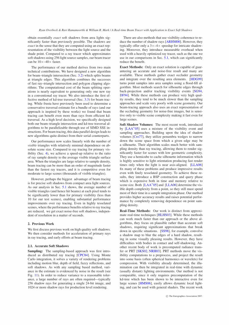
Figure 1: (Top) Beam tracing for primary visibility. (Bot-

tom) Beam tracing for soft shadows.

3. Our Beam Tracing Algorithm

For simplicity of exposition, we describe the general beamtracing algorithm in the context of primary visibility. Thesame ideas extend to secondary shadow beams (see Fig. 1top and bottom).

As shown in Fig. 1(top), we start with one large pyrami-dal beam representing a volume of perspective parallel rays.This beam is recursively split at geometry primitive bound-aries (triangle edges) into a list of beams which is the visiblesurface of the scene.

As with other recent work on fast ray tracing, our scenesare built strictly with triangle primitives, and we use a kd-tree for acceleration. Beams traverse the scene’s kd-tree ina method somewhat similar to standard ray tracing. Visibletriangles found in the kd-tree’s leaf nodes will split the beaminto two lists of sub-beams: hit beams and miss beams. Themiss beams continue scene traversal until they either hit a tri-angle or exit the scene. As the beams split, they form a beamtree (not to be confused with that generated by reflected andrefracted beams in [HH84]).

The primary challenges in making beam tracing efficientare (1) fast beam-triangle intersection routines, and (2) fastmethods to traverse the kd-tree acceleration structure. In thissection, we give a high-level overview of our novel algo-rithms for these tasks. The appendix provides more low-leveldetails and pseudocode—interested readers will wish to fol-low it in parallel with this section.

3.1. Beam Representation

We represent our beams by 3 or 4 corner rays emanatingfrom a common origin. Operations on these corner rays canbe performed in parallel using SIMD instructions availableon most modern processors (similar to [WSBW01]). Pseu-docode for our beam representation is in the appendix. Itis important to note that we represent the ray directions aspoints on some plane as this helps with our efficient triangleintersection algorithm described below. For primary beams,we use the image plane. For secondary point light beams, weuse the plane of the hit triangle, and for area light beams, wecan use a plane on or near the light source. This ensures thataccuracy is measured in the relevant space.



a) b) c) d)

e) f) g) h)

i) j) k) l)

Trivial Cases Needs Split

Split Procedure

Other Split Cases

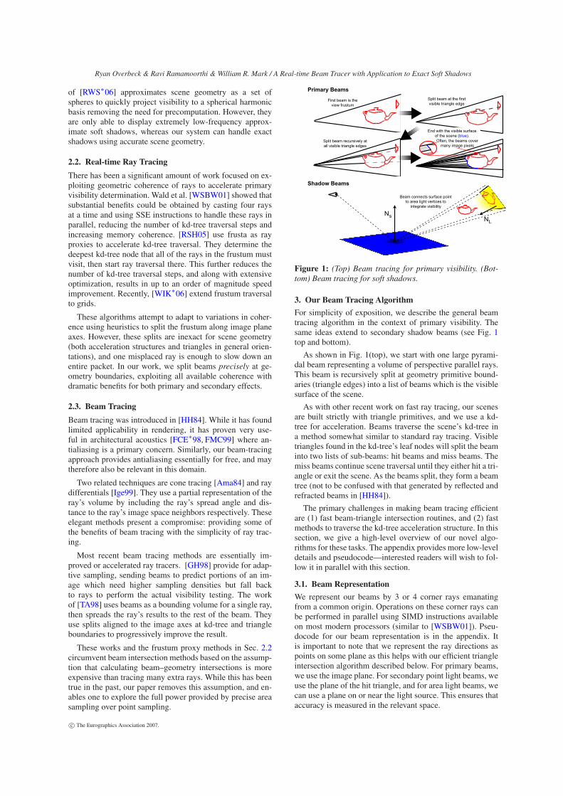
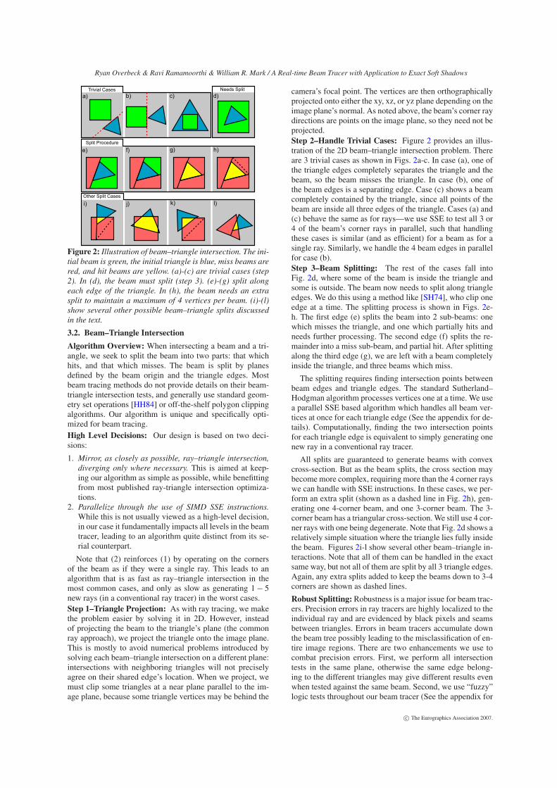
Figure 2: Illustration of beam–triangle intersection. The ini-

tial beam is green, the initial triangle is blue, miss beams are

red, and hit beams are yellow. (a)-(c) are trivial cases (step

2). In (d), the beam must split (step 3). (e)-(g) split along

each edge of the triangle. In (h), the beam needs an extra

split to maintain a maximum of 4 vertices per beam. (i)-(l)

show several other possible beam–triangle splits discussed

in the text.

3.2. Beam–Triangle Intersection

Algorithm Overview: When intersecting a beam and a tri-angle, we seek to split the beam into two parts: that whichhits, and that which misses. The beam is split by planesdefined by the beam origin and the triangle edges. Mostbeam tracing methods do not provide details on their beam-triangle intersection tests, and generally use standard geom-etry set operations [HH84] or off-the-shelf polygon clippingalgorithms. Our algorithm is unique and specifically opti-mized for beam tracing.

High Level Decisions: Our design is based on two deci-sions:

1. Mirror, as closely as possible, ray–triangle intersection,

diverging only where necessary. This is aimed at keep-ing our algorithm as simple as possible, while benefittingfrom most published ray-triangle intersection optimiza-tions.

2. Parallelize through the use of SIMD SSE instructions.

While this is not usually viewed as a high-level decision,in our case it fundamentally impacts all levels in the beamtracer, leading to an algorithm quite distinct from its se-rial counterpart.

Note that (2) reinforces (1) by operating on the cornersof the beam as if they were a single ray. This leads to analgorithm that is as fast as ray–triangle intersection in themost common cases, and only as slow as generating 1− 5new rays (in a conventional ray tracer) in the worst cases.Step 1–Triangle Projection: As with ray tracing, we makethe problem easier by solving it in 2D. However, insteadof projecting the beam to the triangle’s plane (the commonray approach), we project the triangle onto the image plane.This is mostly to avoid numerical problems introduced bysolving each beam–triangle intersection on a different plane:intersections with neighboring triangles will not preciselyagree on their shared edge’s location. When we project, wemust clip some triangles at a near plane parallel to the im-age plane, because some triangle vertices may be behind the

camera’s focal point. The vertices are then orthographicallyprojected onto either the xy, xz, or yz plane depending on theimage plane’s normal. As noted above, the beam’s corner raydirections are points on the image plane, so they need not beprojected.Step 2–Handle Trivial Cases: Figure 2 provides an illus-tration of the 2D beam–triangle intersection problem. Thereare 3 trivial cases as shown in Figs. 2a-c. In case (a), one ofthe triangle edges completely separates the triangle and thebeam, so the beam misses the triangle. In case (b), one ofthe beam edges is a separating edge. Case (c) shows a beamcompletely contained by the triangle, since all points of thebeam are inside all three edges of the triangle. Cases (a) and(c) behave the same as for rays—we use SSE to test all 3 or4 of the beam’s corner rays in parallel, such that handlingthese cases is similar (and as efficient) for a beam as for asingle ray. Similarly, we handle the 4 beam edges in parallelfor case (b).Step 3–Beam Splitting: The rest of the cases fall intoFig. 2d, where some of the beam is inside the triangle andsome is outside. The beam now needs to split along triangleedges. We do this using a method like [SH74], who clip oneedge at a time. The splitting process is shown in Figs. 2e-h. The first edge (e) splits the beam into 2 sub-beams: onewhich misses the triangle, and one which partially hits andneeds further processing. The second edge (f) splits the re-mainder into a miss sub-beam, and partial hit. After splittingalong the third edge (g), we are left with a beam completelyinside the triangle, and three beams which miss.

The splitting requires finding intersection points betweenbeam edges and triangle edges. The standard Sutherland–Hodgman algorithm processes vertices one at a time. We usea parallel SSE based algorithm which handles all beam ver-tices at once for each triangle edge (See the appendix for de-tails). Computationally, finding the two intersection pointsfor each triangle edge is equivalent to simply generating onenew ray in a conventional ray tracer.

All splits are guaranteed to generate beams with convexcross-section. But as the beam splits, the cross section maybecome more complex, requiring more than the 4 corner rayswe can handle with SSE instructions. In these cases, we per-form an extra split (shown as a dashed line in Fig. 2h), gen-erating one 4-corner beam, and one 3-corner beam. The 3-corner beam has a triangular cross-section. We still use 4 cor-ner rays with one being degenerate. Note that Fig. 2d shows arelatively simple situation where the triangle lies fully insidethe beam. Figures 2i-l show several other beam–triangle in-teractions. Note that all of them can be handled in the exactsame way, but not all of them are split by all 3 triangle edges.Again, any extra splits added to keep the beams down to 3-4corners are shown as dashed lines.

Robust Splitting: Robustness is a major issue for beam trac-ers. Precision errors in ray tracers are highly localized to theindividual ray and are evidenced by black pixels and seamsbetween triangles. Errors in beam tracers accumulate downthe beam tree possibly leading to the misclassification of en-tire image regions. There are two enhancements we use tocombat precision errors. First, we perform all intersectiontests in the same plane, otherwise the same edge belong-ing to the different triangles may give different results evenwhen tested against the same beam. Second, we use “fuzzy”logic tests throughout our beam tracer (See the appendix for



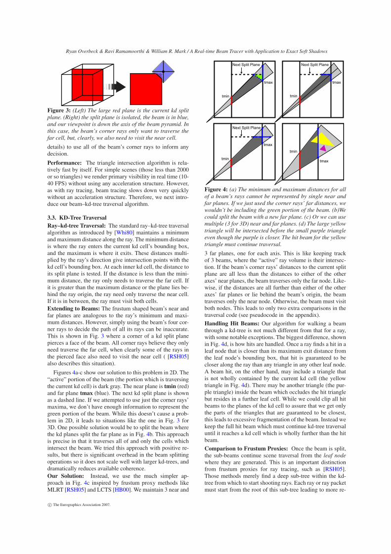
Figure 3: (Left) The large red plane is the current kd split

plane. (Right) the split plane is isolated, the beam is in blue,

and our viewpoint is down the axis of the beam pyramid. In

this case, the beam’s corner rays only want to traverse the

far cell, but, clearly, we also need to visit the near cell.

details) to use all of the beam’s corner rays to inform anydecision.

Performance: The triangle intersection algorithm is rela-tively fast by itself. For simple scenes (those less than 2000or so triangles) we render primary visibility in real time (10-40 FPS) without using any acceleration structure. However,as with ray tracing, beam tracing slows down very quicklywithout an acceleration structure. Therefore, we next intro-duce our beam–kd-tree traversal algorithm.

3.3. KD-Tree Traversal

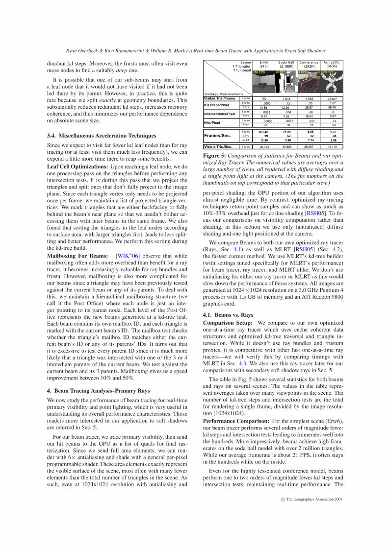
Ray–kd-tree Traversal: The standard ray–kd-tree traversalalgorithm as introduced by [Whi80] maintains a minimumand maximum distance along the ray. The minimum distanceis where the ray enters the current kd cell’s bounding box,and the maximum is where it exits. These distances multi-plied by the ray’s direction give intersection points with thekd cell’s bounding box. At each inner kd cell, the distance toits split plane is tested. If the distance is less than the mini-mum distance, the ray only needs to traverse the far cell. Ifit is greater than the maximum distance or the plane lies be-hind the ray origin, the ray need only traverse the near cell.If it is in between, the ray must visit both cells.Extending to Beams: The frustum shaped beam’s near andfar planes are analogous to the ray’s minimum and maxi-mum distances. However, simply using the beam’s four cor-ner rays to decide the path of all its rays can be inaccurate.This is shown in Fig. 3 where a corner of a kd split planepierces a face of the beam. All corner rays believe they onlyneed traverse the far cell, when clearly some of the rays inthe pierced face also need to visit the near cell ( [RSH05]also describes this situation).

Figures 4a-c show our solution to this problem in 2D. The“active” portion of the beam (the portion which is traversingthe current kd cell) is dark gray. The near plane is tmin (red)and far plane tmax (blue). The next kd split plane is shownas a dashed line. If we attempted to use just the corner rays’maxima, we don’t have enough information to represent thegreen portion of the beam. While this doesn’t cause a prob-lem in 2D, it leads to situations like the one in Fig. 3 for3D. One possible solution would be to split the beam wherethe kd planes split the far plane as in Fig. 4b. This approachis precise in that it traverses all of and only the cells whichintersect the beam. We tried this approach with positive re-sults, but there is significant overhead in the beam splittingoperations so it does not scale well with larger kd-trees, anddramatically reduces available coherence.Our Solution: Instead, we use the much simpler ap-proach in Fig. 4c inspired by frustum proxy methods likeMLRT [RSH05] and LCTS [HB00]. We maintain 3 near and

tmin

tmax

Next Split Plane

tmin

tmax

Next Split Plane

tmin

tmax

Next Split Plane

tmin

tmax

Figure 4: (a) The minimum and maximum distances for all

of a beam’s rays cannot be represented by single near and

far planes. If we just used the corner rays’ far distances, we

wouldn’t be including the green portion of the beam. (b)We

could split the beam with a new far plane. (c) Or we can use

multiple (3 for 3D) near and far planes. (d) The large yellow

triangle will be intersected before the small purple triangle

even though the purple is closer. The hit beam for the yellow

triangle must continue traversal.

3 far planes, one for each axis. This is like keeping trackof 3 beams, where the “active” ray volume is their intersec-tion. If the beam’s corner rays’ distances to the current splitplane are all less than the distances to either of the otheraxes’ near planes, the beam traverses only the far node. Like-wise, if the distances are all further than either of the otheraxes’ far planes or lie behind the beam’s origin, the beamtraverses only the near node. Otherwise, the beam must visitboth nodes. This leads to only two extra comparisons in thetraversal code (see pseudocode in the appendix).

Handling Hit Beams: Our algorithm for walking a beamthrough a kd-tree is not much different from that for a ray,with some notable exceptions. The biggest difference, shownin Fig. 4d, is how hits are handled. Once a ray finds a hit in aleaf node that is closer than its maximum exit distance fromthe leaf node’s bounding box, that hit is guaranteed to becloser along the ray than any triangle in any other leaf node.A beam hit, on the other hand, may include a triangle thatis not wholly contained by the current kd cell (the yellowtriangle in Fig. 4d). There may be another triangle (the pur-ple triangle) inside the beam which occludes the hit trianglebut resides in a further leaf cell. While we could clip all hitbeams to the planes of the kd cell to assure that we get onlythe parts of the triangles that are guaranteed to be closest,this leads to excessive fragmentation of the beam. Instead wekeep the full hit beam which must continue kd-tree traversaluntil it reaches a kd cell which is wholly further than the hitbeam.

Comparison to Frustum Proxies: Once the beam is split,the sub-beams continue scene traversal from the leaf node

where they are generated. This is an important distinctionfrom frustum proxies for ray tracing, such as [RSH05].Those methods merely find a deep sub-tree within the kd-tree from which to start shooting rays. Each ray or ray packetmust start from the root of this sub-tree leading to more re-



dundant kd steps. Moreover, the frusta must often visit evenmore nodes to find a suitably deep one.

It is possible that one of our sub-beams may start froma leaf node that it would not have visited if it had not beenled there by its parent. However, in practice, this is quiterare because we split exactly at geometry boundaries. Thissubstantially reduces redundant kd steps, increases memorycoherence, and thus minimizes our performance dependenceon absolute scene size.

3.4. Miscellaneous Acceleration Techniques

Since we expect to visit far fewer kd leaf nodes than for raytracing (or at least visit them much less frequently), we canexpend a little more time there to reap some benefits.

Leaf Cell Optimizations: Upon reaching a leaf node, we doone processing pass on the triangles before performing anyintersection tests. It is during this pass that we project thetriangles and split ones that don’t fully project to the imageplane. Since each triangle vertex only needs to be projectedonce per frame, we maintain a list of projected triangle ver-tices. We mark triangles that are either backfacing or fullybehind the beam’s near plane so that we needn’t bother ac-cessing them with later beams in the same frame. We alsofound that sorting the triangles in the leaf nodes accordingto surface area, with larger triangles first, leads to less split-ting and better performance. We perform this sorting duringthe kd-tree build.

Mailboxing For Beams: [WIK∗06] observe that whilemailboxing often adds more overhead than benefit for a raytracer, it becomes increasingly valuable for ray bundles andfrusta. However, mailboxing is also more complicated forour beams since a triangle may have been previously testedagainst the current beam or any of its parents. To deal withthis, we maintain a hierarchical mailboxing structure (wecall it the Post Office) where each node is just an inte-ger pointing to its parent node. Each level of the Post Of-fice represents the new beams generated at a kd-tree leaf.Each beam contains its own mailbox ID, and each triangle ismarked with the current beam’s ID. The mailbox test checkswhether the triangle’s mailbox ID matches either the cur-rent beam’s ID or any of its parents’ IDs. It turns out thatit is excessive to test every parent ID since it is much morelikely that a triangle was intersected with one of the 3 or 4immediate parents of the current beam. We test against thecurrent beam and its 3 parents. Mailboxing gives us a speedimprovement between 10% and 50%.

4. Beam Tracing Analysis–Primary Rays

We now study the performance of beam tracing for real-timeprimary visibility and point lighting, which is very useful inunderstanding its overall performance characteristics. Thosereaders more interested in our application to soft shadowsare referred to Sec. 5.

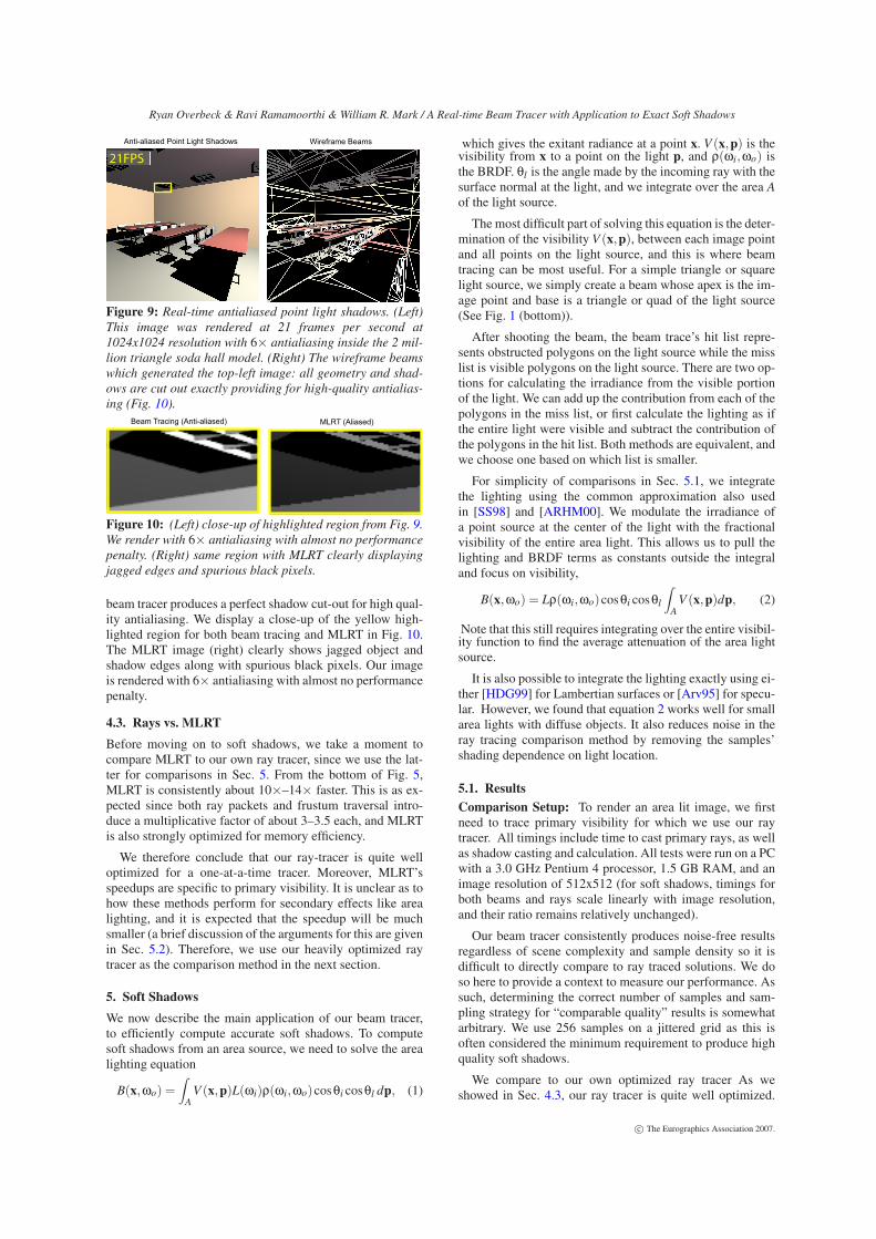
For our beam tracer, we trace primary visibility, then sendour hit beams to the GPU as a list of quads for final ras-terization. Since we send full area elements, we can ren-der with 6× antialiasing and shade with a general per-pixelprogrammable shader. These area elements exactly representthe visible surface of the scene, most often with many fewerelements than the total number of triangles in the scene. Assuch, even at 1024x1024 resolution with antialiasing and

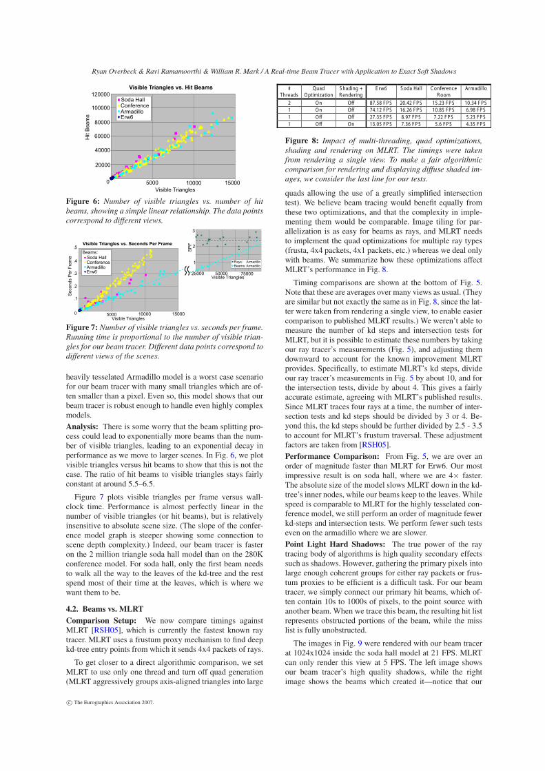
S cene# T rianglesThumbnail

Average Meas urements

E rw6(816)

S oda Hall Conference Armadillo

Beams

Beams

R ays

Beams

R ays

Beams

R ays

Beams

R ays

MLR T

Beams

150 4,6021,536 25,647Visible Tris./Frame

KD Steps/Pixel

Intersections/Pixel

Hits/Pixel

Frames/Sec.

Visible Tris./Sec.

.0085 .13 .30 1.07

13.86 25.6742.36 46.46

.0033 .064 .48 .6

6.81 16.344.29 5.67

.95 .98 .91 .99

.00096 .0097 .027 .14

169.49

.99 .52 .52

1.72

.44

21.28 5.56

12.99 5.56 7.14 5.99

25,424 32,686 25,587 44,113

180 FPS 25 FPS 4 FPS 0.35 FPS

(2,195K) (282K) (345K)

Figure 5: Comparison of statistics for Beams and our opti-

mized Ray Tracer. The numerical values are averages over a

large number of views, all rendered with diffuse shading and

a single point light at the camera. (The fps numbers on the

thumbnails on top correspond to that particular view.)

per-pixel shading, the GPU portion of our algorithm usesalmost negligible time. By contrast, optimized ray-tracingtechniques return point samples and can show as much as10%-33% overhead just for cosine shading [RSH05]. To fo-cus our comparisons on visibility computation rather thanshading, in this section we use only (antialiased) diffuseshading and one light positioned at the camera.

We compare Beams to both our own optimized ray tracer(Rays, Sec. 4.1) as well as MLRT [RSH05] (Sec. 4.2),the fastest current method. We use MLRT’s kd-tree builder(with settings tuned specifically for MLRT’s performance)for beam tracer, ray tracer, and MLRT alike. We don’t useantialiasing for either our ray tracer or MLRT as this wouldslow down the performance of those systems. All images aregenerated at 1024×1024 resolution on a 3.0 GHz Pentium 4processor with 1.5 GB of memory and an ATI Radeon 9800graphics card.

4.1. Beams vs. Rays

Comparison Setup: We compare to our own optimizedone-at-a-time ray tracer which uses cache coherent datastructures and optimized kd-tree traversal and triangle in-tersection. While it doesn’t use ray bundles and frustumproxies, it is competitive with other fast one-at-a-time raytracers—we will verify this by comparing timings withMLRT in Sec. 4.3. We also use this ray tracer later for ourcomparisons with secondary soft shadow rays in Sec. 5.

The table in Fig. 5 shows several statistics for both beamsand rays on several scenes. The values in the table repre-sent averages taken over many viewpoints in the scene. Thenumber of kd-tree steps and intersection tests are the totalfor rendering a single frame, divided by the image resolu-tion (1024x1024).

Performance Comparison: For the simplest scene (Erw6),our beam tracer performs several orders of magnitude fewerkd steps and intersection tests leading to framerates well intothe hundreds. More impressively, beams achieve high fram-erates on the soda hall model with over 2 million triangles.While our average framerate is about 21 FPS, it often staysin the hundreds while on the inside.

Even for the highly tesselated conference model, beamsperform one to two orders of magnitude fewer kd steps andintersection tests, maintaining real-time performance. The



Visible Triangles vs. Hit Beams

Visible Triangles

Hit B

eam

s

5000 10000 150000

20000

40000

60000

80000

100000

120000Soda HallConference

Erw6Armadillo

Figure 6: Number of visible triangles vs. number of hit

beams, showing a simple linear relationship. The data points

correspond to different views.

0

Visible Triangles

Visible Triangles vs. Seconds Per Frame

5000 10000 15000

Se

co

nd

s P

er

Fra

me

.1

.2

.3

.4

.5

Soda HallConference

Erw6Armadillo

Beams:

Rays: Armadillo

Beams: Armadillo

25000 50000 75000

1

2

3

Visible Triangles

SP

F

Figure 7: Number of visible triangles vs. seconds per frame.

Running time is proportional to the number of visible trian-

gles for our beam tracer. Different data points correspond to

different views of the scenes.

heavily tesselated Armadillo model is a worst case scenariofor our beam tracer with many small triangles which are of-ten smaller than a pixel. Even so, this model shows that ourbeam tracer is robust enough to handle even highly complexmodels.

Analysis: There is some worry that the beam splitting pro-cess could lead to exponentially more beams than the num-ber of visible triangles, leading to an exponential decay inperformance as we move to larger scenes. In Fig. 6, we plotvisible triangles versus hit beams to show that this is not thecase. The ratio of hit beams to visible triangles stays fairlyconstant at around 5.5–6.5.

Figure 7 plots visible triangles per frame versus wall-clock time. Performance is almost perfectly linear in thenumber of visible triangles (or hit beams), but is relativelyinsensitive to absolute scene size. (The slope of the confer-ence model graph is steeper showing some connection toscene depth complexity.) Indeed, our beam tracer is fasteron the 2 million triangle soda hall model than on the 280Kconference model. For soda hall, only the first beam needsto walk all the way to the leaves of the kd-tree and the restspend most of their time at the leaves, which is where wewant them to be.

4.2. Beams vs. MLRT

Comparison Setup: We now compare timings againstMLRT [RSH05], which is currently the fastest known raytracer. MLRT uses a frustum proxy mechanism to find deepkd-tree entry points from which it sends 4x4 packets of rays.

To get closer to a direct algorithmic comparison, we setMLRT to use only one thread and turn off quad generation(MLRT aggressively groups axis-aligned triangles into large

#Threads

QuadOptimization

S hading +R endering

E rw6 S oda Hall ConferenceR oom

Armadillo

2 On O� 87.58 FPS 20.42 FPS 15.23 FPS 10.34 FPS

1 On O� 74.12 FPS 16.26 FPS 10.85 FPS 6.98 FPS

1 O� Off 27.35 FPS 8.97 FPS 7.22 FPS 5.23 FPS

1 O� On 13.05 FPS 7.36 FPS 5.6 FPS 4.35 FPS

Figure 8: Impact of multi-threading, quad optimizations,

shading and rendering on MLRT. The timings were taken

from rendering a single view. To make a fair algorithmic

comparison for rendering and displaying diffuse shaded im-

ages, we consider the last line for our tests.

quads allowing the use of a greatly simplified intersectiontest). We believe beam tracing would benefit equally fromthese two optimizations, and that the complexity in imple-menting them would be comparable. Image tiling for par-allelization is as easy for beams as rays, and MLRT needsto implement the quad optimizations for multiple ray types(frusta, 4x4 packets, 4x1 packets, etc.) whereas we deal onlywith beams. We summarize how these optimizations affectMLRT’s performance in Fig. 8.

Timing comparisons are shown at the bottom of Fig. 5.Note that these are averages over many views as usual. (Theyare similar but not exactly the same as in Fig. 8, since the lat-ter were taken from rendering a single view, to enable easiercomparison to published MLRT results.) We weren’t able tomeasure the number of kd steps and intersection tests forMLRT, but it is possible to estimate these numbers by takingour ray tracer’s measurements (Fig. 5), and adjusting themdownward to account for the known improvement MLRTprovides. Specifically, to estimate MLRT’s kd steps, divideour ray tracer’s measurements in Fig. 5 by about 10, and forthe intersection tests, divide by about 4. This gives a fairlyaccurate estimate, agreeing with MLRT’s published results.Since MLRT traces four rays at a time, the number of inter-section tests and kd steps should be divided by 3 or 4. Be-yond this, the kd steps should be further divided by 2.5 - 3.5to account for MLRT’s frustum traversal. These adjustmentfactors are taken from [RSH05].

Performance Comparison: From Fig. 5, we are over anorder of magnitude faster than MLRT for Erw6. Our mostimpressive result is on soda hall, where we are 4× faster.The absolute size of the model slows MLRT down in the kd-tree’s inner nodes, while our beams keep to the leaves. Whilespeed is comparable to MLRT for the highly tesselated con-ference model, we still perform an order of magnitude fewerkd-steps and intersection tests. We perform fewer such testseven on the armadillo where we are slower.

Point Light Hard Shadows: The true power of the raytracing body of algorithms is high quality secondary effectssuch as shadows. However, gathering the primary pixels intolarge enough coherent groups for either ray packets or frus-tum proxies to be efficient is a difficult task. For our beamtracer, we simply connect our primary hit beams, which of-ten contain 10s to 1000s of pixels, to the point source withanother beam. When we trace this beam, the resulting hit listrepresents obstructed portions of the beam, while the misslist is fully unobstructed.

The images in Fig. 9 were rendered with our beam tracerat 1024x1024 inside the soda hall model at 21 FPS. MLRTcan only render this view at 5 FPS. The left image showsour beam tracer’s high quality shadows, while the rightimage shows the beams which created it—notice that our



21FPS

Anti-aliased Point Light Shadows Wireframe Beams

Figure 9: Real-time antialiased point light shadows. (Left)

This image was rendered at 21 frames per second at

1024x1024 resolution with 6× antialiasing inside the 2 mil-

lion triangle soda hall model. (Right) The wireframe beams

which generated the top-left image: all geometry and shad-

ows are cut out exactly providing for high-quality antialias-

ing (Fig. 10).

Beam Tracing (Anti-aliased) MLRT (Aliased)

Figure 10: (Left) close-up of highlighted region from Fig. 9.

We render with 6× antialiasing with almost no performance

penalty. (Right) same region with MLRT clearly displaying

jagged edges and spurious black pixels.

beam tracer produces a perfect shadow cut-out for high qual-ity antialiasing. We display a close-up of the yellow high-lighted region for both beam tracing and MLRT in Fig. 10.The MLRT image (right) clearly shows jagged object andshadow edges along with spurious black pixels. Our imageis rendered with 6× antialiasing with almost no performancepenalty.

4.3. Rays vs. MLRT

Before moving on to soft shadows, we take a moment tocompare MLRT to our own ray tracer, since we use the lat-ter for comparisons in Sec. 5. From the bottom of Fig. 5,MLRT is consistently about 10×–14× faster. This is as ex-pected since both ray packets and frustum traversal intro-duce a multiplicative factor of about 3–3.5 each, and MLRTis also strongly optimized for memory efficiency.

We therefore conclude that our ray-tracer is quite welloptimized for a one-at-a-time tracer. Moreover, MLRT’sspeedups are specific to primary visibility. It is unclear as tohow these methods perform for secondary effects like arealighting, and it is expected that the speedup will be muchsmaller (a brief discussion of the arguments for this are givenin Sec. 5.2). Therefore, we use our heavily optimized raytracer as the comparison method in the next section.

5. Soft Shadows

We now describe the main application of our beam tracer,to efficiently compute accurate soft shadows. To computesoft shadows from an area source, we need to solve the arealighting equation

B(x,ωo) =∫

AV (x,p)L(ωi)ρ(ωi,ωo)cosθi cosθl dp, (1)

which gives the exitant radiance at a point x. V (x,p) is thevisibility from x to a point on the light p, and ρ(ωi,ωo) isthe BRDF. θl is the angle made by the incoming ray with thesurface normal at the light, and we integrate over the area A

of the light source.

The most difficult part of solving this equation is the deter-mination of the visibility V (x,p), between each image pointand all points on the light source, and this is where beamtracing can be most useful. For a simple triangle or squarelight source, we simply create a beam whose apex is the im-age point and base is a triangle or quad of the light source(See Fig. 1 (bottom)).

After shooting the beam, the beam trace’s hit list repre-sents obstructed polygons on the light source while the misslist is visible polygons on the light source. There are two op-tions for calculating the irradiance from the visible portionof the light. We can add up the contribution from each of thepolygons in the miss list, or first calculate the lighting as ifthe entire light were visible and subtract the contribution ofthe polygons in the hit list. Both methods are equivalent, andwe choose one based on which list is smaller.

For simplicity of comparisons in Sec. 5.1, we integratethe lighting using the common approximation also usedin [SS98] and [ARHM00]. We modulate the irradiance ofa point source at the center of the light with the fractionalvisibility of the entire area light. This allows us to pull thelighting and BRDF terms as constants outside the integraland focus on visibility,

B(x,ωo) = Lρ(ωi,ωo)cosθi cosθl

∫A

V (x,p)dp, (2)

Note that this still requires integrating over the entire visibil-ity function to find the average attenuation of the area lightsource.

It is also possible to integrate the lighting exactly using ei-ther [HDG99] for Lambertian surfaces or [Arv95] for specu-lar. However, we found that equation 2 works well for smallarea lights with diffuse objects. It also reduces noise in theray tracing comparison method by removing the samples’shading dependence on light location.

5.1. Results

Comparison Setup: To render an area lit image, we firstneed to trace primary visibility for which we use our raytracer. All timings include time to cast primary rays, as wellas shadow casting and calculation. All tests were run on a PCwith a 3.0 GHz Pentium 4 processor, 1.5 GB RAM, and animage resolution of 512x512 (for soft shadows, timings forboth beams and rays scale linearly with image resolution,and their ratio remains relatively unchanged).

Our beam tracer consistently produces noise-free resultsregardless of scene complexity and sample density so it isdifficult to directly compare to ray traced solutions. We doso here to provide a context to measure our performance. Assuch, determining the correct number of samples and sam-pling strategy for “comparable quality” results is somewhatarbitrary. We use 256 samples on a jittered grid as this isoften considered the minimum requirement to produce highquality soft shadows.

We compare to our own optimized ray tracer As weshowed in Sec. 4.3, our ray tracer is quite well optimized.



9 Seconds / 25 Shadow Rays

3 Seconds

Ray T

racin

g:

Com

para

ble

Tim

eB

eam

Tra

cin

g:

Re

fere

nce Q

ualit

y

81 Seconds

With Jittering Without Jittering

108 Seconds

Ra

y T

racin

g: C

om

pa

rab

le Q

ualit

y

256 S

hado

w R

ays

5 Seconds / 9 Shadow Rays 1.84 Seconds / 4 Shadow Rays 3 Seconds / 4 Shadow Rays

79 Seconds 99 Seconds

1.78 Seconds9 Seconds5 Seconds

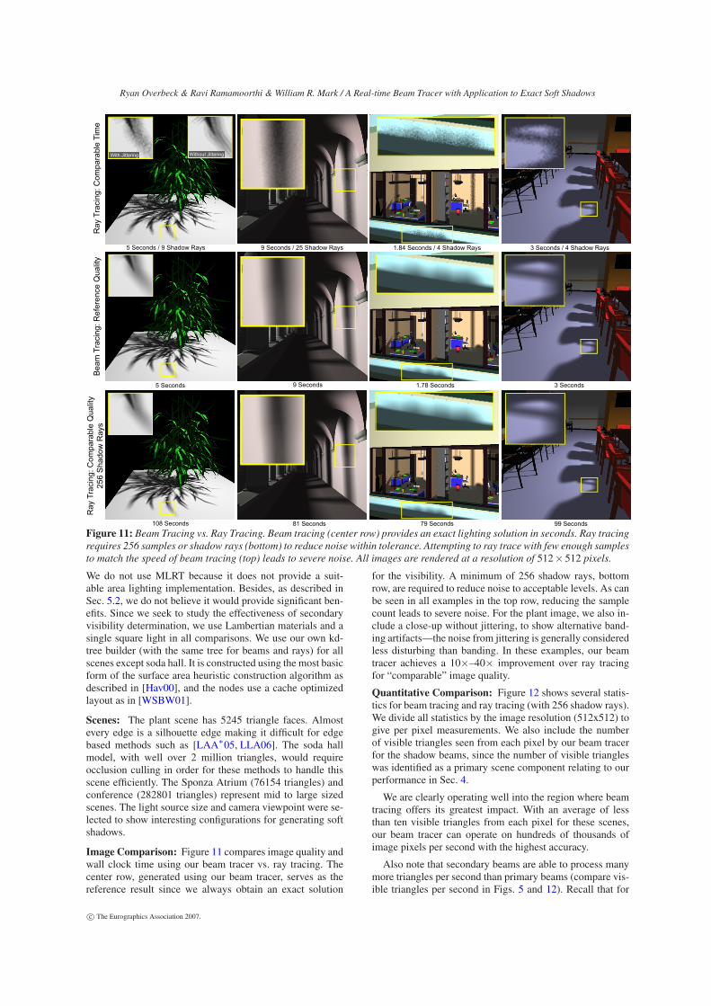
Figure 11: Beam Tracing vs. Ray Tracing. Beam tracing (center row) provides an exact lighting solution in seconds. Ray tracing

requires 256 samples or shadow rays (bottom) to reduce noise within tolerance. Attempting to ray trace with few enough samples

to match the speed of beam tracing (top) leads to severe noise. All images are rendered at a resolution of 512×512 pixels.

We do not use MLRT because it does not provide a suit-able area lighting implementation. Besides, as described inSec. 5.2, we do not believe it would provide significant ben-efits. Since we seek to study the effectiveness of secondaryvisibility determination, we use Lambertian materials and asingle square light in all comparisons. We use our own kd-tree builder (with the same tree for beams and rays) for allscenes except soda hall. It is constructed using the most basicform of the surface area heuristic construction algorithm asdescribed in [Hav00], and the nodes use a cache optimizedlayout as in [WSBW01].

Scenes: The plant scene has 5245 triangle faces. Almostevery edge is a silhouette edge making it difficult for edgebased methods such as [LAA∗05, LLA06]. The soda hallmodel, with well over 2 million triangles, would requireocclusion culling in order for these methods to handle thisscene efficiently. The Sponza Atrium (76154 triangles) andconference (282801 triangles) represent mid to large sizedscenes. The light source size and camera viewpoint were se-lected to show interesting configurations for generating softshadows.

Image Comparison: Figure 11 compares image quality andwall clock time using our beam tracer vs. ray tracing. Thecenter row, generated using our beam tracer, serves as thereference result since we always obtain an exact solution

for the visibility. A minimum of 256 shadow rays, bottomrow, are required to reduce noise to acceptable levels. As canbe seen in all examples in the top row, reducing the samplecount leads to severe noise. For the plant image, we also in-clude a close-up without jittering, to show alternative band-ing artifacts—the noise from jittering is generally consideredless disturbing than banding. In these examples, our beamtracer achieves a 10×–40× improvement over ray tracingfor “comparable” image quality.

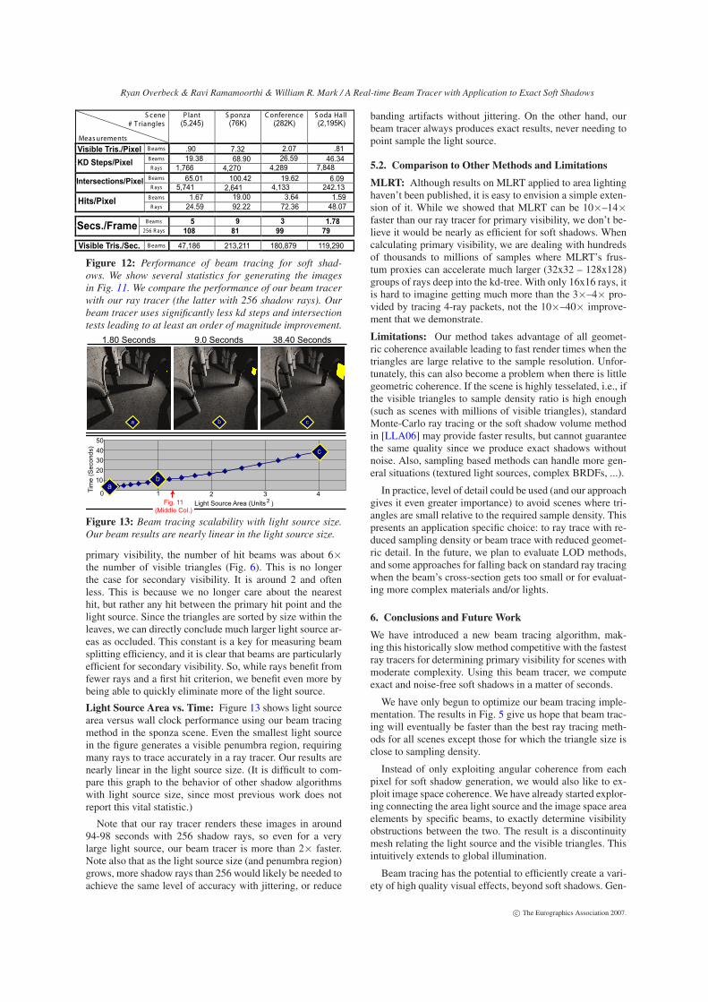
Quantitative Comparison: Figure 12 shows several statis-tics for beam tracing and ray tracing (with 256 shadow rays).We divide all statistics by the image resolution (512x512) togive per pixel measurements. We also include the numberof visible triangles seen from each pixel by our beam tracerfor the shadow beams, since the number of visible triangleswas identified as a primary scene component relating to ourperformance in Sec. 4.

We are clearly operating well into the region where beamtracing offers its greatest impact. With an average of lessthan ten visible triangles from each pixel for these scenes,our beam tracer can operate on hundreds of thousands ofimage pixels per second with the highest accuracy.

Also note that secondary beams are able to process manymore triangles per second than primary beams (compare vis-ible triangles per second in Figs. 5 and 12). Recall that for



S cene# T riangles

Meas urements

P lant S ponza Conference S oda Hall

Beams

Beams

R ays

Beams

R ays

Beams

R ays

Beams

256 R ays

Beams

(76K) (282K)(5,245) (2,195K)

2.077.32.90 .81

19.38

1,766

65.015,741

68.90

4,270

100.42

2,641

26.59

4,289

19.624,133

6.09

46.34

242.13

7,848

1.67

24.59

19.00

92.22

3.64

72.36

1.59

48.07

47,186 213,211 180,879 119,290

5

108

9

81

3

99

1.78

79

KD Steps/Pixel

Intersections/Pixel

Hits/Pixel

Visible Tris./Sec.

Secs./Frame

Visible Tris./Pixel

Figure 12: Performance of beam tracing for soft shad-

ows. We show several statistics for generating the images

in Fig. 11. We compare the performance of our beam tracer

with our ray tracer (the latter with 256 shadow rays). Our

beam tracer uses significantly less kd steps and intersection

tests leading to at least an order of magnitude improvement.

10 2 3 4

10

20

30

40

50

Light Source Area (Units )2

Tim

e (

Se

conds)

ab

c

Fig. 11

(Middle Col.)

a b c

1.80 Seconds 9.0 Seconds 38.40 Seconds

Figure 13: Beam tracing scalability with light source size.

Our beam results are nearly linear in the light source size.

primary visibility, the number of hit beams was about 6×the number of visible triangles (Fig. 6). This is no longerthe case for secondary visibility. It is around 2 and oftenless. This is because we no longer care about the nearesthit, but rather any hit between the primary hit point and thelight source. Since the triangles are sorted by size within theleaves, we can directly conclude much larger light source ar-eas as occluded. This constant is a key for measuring beamsplitting efficiency, and it is clear that beams are particularlyefficient for secondary visibility. So, while rays benefit fromfewer rays and a first hit criterion, we benefit even more bybeing able to quickly eliminate more of the light source.

Light Source Area vs. Time: Figure 13 shows light sourcearea versus wall clock performance using our beam tracingmethod in the sponza scene. Even the smallest light sourcein the figure generates a visible penumbra region, requiringmany rays to trace accurately in a ray tracer. Our results arenearly linear in the light source size. (It is difficult to com-pare this graph to the behavior of other shadow algorithmswith light source size, since most previous work does notreport this vital statistic.)

Note that our ray tracer renders these images in around94-98 seconds with 256 shadow rays, so even for a verylarge light source, our beam tracer is more than 2× faster.Note also that as the light source size (and penumbra region)grows, more shadow rays than 256 would likely be needed toachieve the same level of accuracy with jittering, or reduce

banding artifacts without jittering. On the other hand, ourbeam tracer always produces exact results, never needing topoint sample the light source.

5.2. Comparison to Other Methods and Limitations

MLRT: Although results on MLRT applied to area lightinghaven’t been published, it is easy to envision a simple exten-sion of it. While we showed that MLRT can be 10×–14×faster than our ray tracer for primary visibility, we don’t be-lieve it would be nearly as efficient for soft shadows. Whencalculating primary visibility, we are dealing with hundredsof thousands to millions of samples where MLRT’s frus-tum proxies can accelerate much larger (32x32 – 128x128)groups of rays deep into the kd-tree. With only 16x16 rays, itis hard to imagine getting much more than the 3×–4× pro-vided by tracing 4-ray packets, not the 10×–40× improve-ment that we demonstrate.

Limitations: Our method takes advantage of all geomet-ric coherence available leading to fast render times when thetriangles are large relative to the sample resolution. Unfor-tunately, this can also become a problem when there is littlegeometric coherence. If the scene is highly tesselated, i.e., ifthe visible triangles to sample density ratio is high enough(such as scenes with millions of visible triangles), standardMonte-Carlo ray tracing or the soft shadow volume methodin [LLA06] may provide faster results, but cannot guaranteethe same quality since we produce exact shadows withoutnoise. Also, sampling based methods can handle more gen-eral situations (textured light sources, complex BRDFs, ...).

In practice, level of detail could be used (and our approachgives it even greater importance) to avoid scenes where tri-angles are small relative to the required sample density. Thispresents an application specific choice: to ray trace with re-duced sampling density or beam trace with reduced geomet-ric detail. In the future, we plan to evaluate LOD methods,and some approaches for falling back on standard ray tracingwhen the beam’s cross-section gets too small or for evaluat-ing more complex materials and/or lights.

6. Conclusions and Future Work

We have introduced a new beam tracing algorithm, mak-ing this historically slow method competitive with the fastestray tracers for determining primary visibility for scenes withmoderate complexity. Using this beam tracer, we computeexact and noise-free soft shadows in a matter of seconds.

We have only begun to optimize our beam tracing imple-mentation. The results in Fig. 5 give us hope that beam trac-ing will eventually be faster than the best ray tracing meth-ods for all scenes except those for which the triangle size isclose to sampling density.

Instead of only exploiting angular coherence from eachpixel for soft shadow generation, we would also like to ex-ploit image space coherence. We have already started explor-ing connecting the area light source and the image space areaelements by specific beams, to exactly determine visibilityobstructions between the two. The result is a discontinuitymesh relating the light source and the visible triangles. Thisintuitively extends to global illumination.

Beam tracing has the potential to efficiently create a vari-ety of high quality visual effects, beyond soft shadows. Gen-



erating specular reflections and caustics is one promising di-rection. In fact, the work of [LWY∗07], developed concur-rently with ours, extends beams to nonlinear reflection andrefraction transformations. Caustics often require millions ofrays to get a sampling density high enough to remove noisefrom the image. Just as for soft shadows, beams may be rel-atively insensitive to this problem.

Beam tracing has largely been ignored by the render-ing community recently due to its perceived poor perfor-mance characteristics. Our work proves that this perceptionis largely undeserved, and we have only provided a peek intothe true potential for high speed beam tracing. We hope thiswork encourages more attention in this promising direction.

Acknowledgements

This research was funded in part by NSF grants #0305322,#0446916, and #0546236, a research grant from Intel Corpora-tion, a Sloan Research Fellowship, and an ONR Young InvestigatorAward N00014-17-1-0900. We would also like to thank AlexanderReshetov for MLRT code and scenes, and Aner Ben-Artzi and KevinEgan for many helpful discussions. The Sponza Atrium model isprovided courtesy of Marko Dabrovic.

References

[Ama84] AMANATIDES J.: Ray tracing with cones. In SIG-

GRAPH 84 (1984), pp. 129–135.[ARHM00] AGRAWALA M., RAMAMOORTHI R., HEIRICH

A., MOLL L.: Efficient image-based methods for render-ing soft shadows. In SIGGRAPH 00 (2000), pp. 375–384.

[Arv95] ARVO J.: Applications of irradiance tensors to thesimulation of non-Lambertian phenomena. In SIGGRAPH

95 (1995), pp. 335–342.[BEL∗07] BOULOS S., EDWARDS D., LACEWELL J. D.,

KNISS J., KAUTZ J., SHIRLEY P., WALD I.: Packet-basedWhitted and Distribution Ray Tracing. In Proc. Graphics

Interface (May 2007).[CPC84] COOK R. L., PORTER T., CARPENTER L.: Dis-

tributed ray tracing. In SIGGRAPH 84 (1984), pp. 137–145.

[Cro77] CROW F. C.: Shadow algorithms for computergraphics. In SIGGRAPH 77 (1977), pp. 242–248.

[DF94] DRETTAKIS G., FIUME E.: A fast shadow algorithmfor area light sources using backprojection. In SIGGRAPH

94 (1994), pp. 223–230.[FCE∗98] FUNKHOUSER T., CARLBOM I., ELKO G., PIN-

GALI G., SONDHI M., WEST J.: A beam tracing approachto acoustic modeling for interactive virtual environments.In SIGGRAPH 98 (1998), pp. 21–32.

[FMC99] FUNKHOUSER T. A., MIN P., CARLBOM I.: Real-time acoustic modeling for distributed virtual environ-ments. In SIGGRAPH 99 (1999), pp. 365–374.

[GH98] GHAZANFARPOUR D., HASENFRATZ J.-M.: A beamtracing method with precise antialiasing for polyhedralscenes. Computers and Graphics 22, 1 (1998), 103–115.

[Hav00] HAVRAN V.: Heuristic Ray Shooting Algorithms. PhDthesis, Department of Computer Science and Engineering,Faculty of Electrical Engineering, Czech Technical Uni-versity in Prague, November 2000.

[HB00] HAVRAN V., BITTNER J.: LCTS: Ray shooting us-ing longest common traversal sequences. Computer Graph-

ics Forum 19, 3 (2000), 59.

[HDG99] HART D., DUTRE; P., GREENBERG D. P.: Directillumination with lazy visibility evaluation. In SIGGRAPH

99 (1999), pp. 147–154.[HH84] HECKBERT P. S., HANRAHAN P.: Beam tracing

polygonal objects. In SIGGRAPH 84 (1984), pp. 119–127.[HLHS03] HASENFRATZ J.-M., LAPIERRE M.,

HOLZSCHUCH N., SILLION F.: A survey of real-timesoft shadow algorithms. Computer Graphics Forum 22, 4(Dec. 2003), 753–774. State-of-the-Art Reviews.

[HMS06] HUNT W., MARK W. R., STOLL G.: Fast kd-treeconstruction with an adaptive error-bounded heuristic. In2006 IEEE Symposium on Interactive Ray Tracing (2006).

[Ige99] IGEHY H.: Tracing ray differentials. In SIGGRAPH

99 (1999), pp. 179–186.[LAA∗05] LAINE S., AILA T., ASSARSSON U., LEHTINEN

J., AKENINE-MÖLLER T.: Soft shadow volumes for raytracing. ACM TOG SIGGRAPH 05 24, 3 (2005), 1156–1165.

[LLA06] LEHTINEN J., LAINE S., AILA T.: An improvedphysically-based soft shadow volume algorithm. Computer

Graphics Forum 25, 3 (2006), 303–312.[LWY∗07] LIU B., WEI L., YANG X., XU Y., GUO B.: Non-

linear Beam Tracing on a GPU. Tech. Rep. MSR-TR-2007-34, Microsoft Research, 2007.

[NRH03] NG R., RAMAMOORTHI R., HANRAHAN P.: All-frequency shadows using non-linear wavelet lighting ap-proximation. ACM TOG SIGGRAPH 03 22, 3 (2003), 376–381.

[RSH05] RESHETOV A., SOUPIKOV A., HURLEY J.: Multi-level ray tracing algorithm. ACM TOG SIGGRAPH 05 24, 3(2005), 1176–1185.

[RWS∗06] REN Z., WANG R., SNYDER J., ZHOU K., LIU X.,SUN B., SLOAN P.-P., BAO H., PENG Q., GUO B.: Real-time soft shadows in dynamic scenes using spherical har-monic exponentiation. ACM TOG SIGGRAPH 06 (2006),977–986.

[SG94] STEWART A. J., GHALI S.: Fast computation ofshadow boundaries using spatial coherence and backpro-jections. In SIGGRAPH 94 (1994), pp. 231–238.

[SH74] SUTHERLAND I. E., HODGMAN G. W.: Reentrantpolygon clipping. Commun. ACM 17, 1 (1974), 32–42.

[SKS02] SLOAN P., KAUTZ J., SNYDER J.: Precomputed ra-diance transfer for real-time rendering in dynamic, low-frequency lighting environments. ACM TOG SIGGRAPH

02 21, 3 (2002), 527–536.[SS98] SOLER C., SILLION F.: Fast calculation of soft

shadow textures using convolution. In SIGGRAPH 98

(1998), pp. 321–332.[SWZ96] SHIRLEY P., WANG C., ZIMMERMAN K.: Monte

carlo techniques for direct lighting calculations. ACM TOG

15, 1 (1996), 1–36.[TA98] TELLER S., ALEX J.: Frustum Casting for Progressive,

Interactive Rendering. Tech. Rep. MIT/LCS/TR-740, 1998.[Whi80] WHITTED T.: An improved illumination model for

shaded display. Communications of the ACM 23, 6 (1980),343–349.

[WIK∗06] WALD I., IZE T., KENSLER A., KNOLL A.,PARKER S. G.: Ray tracing animated scenes using coher-ent grid traversal. ACM TOG SIGGRAPH 06 (2006), 485–493.

[WSBW01] WALD I., SLUSALLEK P., BENTHIN C., WAGNER

M.: Interactive rendering with coherent ray tracing. Com-

puter Graphics Forum 20, 3 (2001), 153–164.



Appendix A: Algorithm Details

In the following subsections we give low-level details and pseu-docode for beam–triangle intersection and kd-tree traversal.

Beam RepresentationA 3D ray is defined by an origin, a direction, and a maximum dis-tance along the ray (the hit distance once a hit is found for a pri-mary ray). We represent a beam as four corner rays. In our work,we exploit the SSE intrinsics, a library of macros, for ease of imple-mentation. The atomic datatype used by these macros is the __m128structure, which packs 4 32–bit single precision floating point valuestogether into one variable. Most standard floating point operationscan be performed on all four variables in parallel. In the followingpseudocode examples we will replace these intrinsics with more in-tuitively meaningful terminology (__m128 ≡ float4) and operators.

Instead of representing a beam as an array of four rays (Arrayof Structures or AOS), it is more efficient to interleave the rays’members into Structures of Arrays (SOA):

// SOA representation of 4 3D vectors

struct soavec3 {

float4 x,y,z;

};

// A 3D Beam is defined by 4 corner rays which meet at a point.

struct Beam {

soavec3 Origin; // Beam origin

soavec3 Dirs; // Beam corner’s directions

soavec3 InvDirs; // Inverse of directions

float4 MinDist; // Min distance along corner rays

float4 MaxDist; // Max distance along corner rays

int Signs[3]; // Signs of Dir

int pad; // Keep the structure aligned

};

Triangle IntersectionIn the image plane, the beam’s 3 or 4 corner points can all lie on oneside of a triangle edge or be split in two. Using SSE2 instructions,we can simultaneously test the 4 beam points against the triangleedge, and store the result in a 4-bit mask:

soavec2 diff = BeamPoints2D - triPoint2D;

float4 dotval = dot( diff,triPerp2D );

bool4 mask = (dotval < 0);

This mask tells us on which side of the plane each of the 4 pointsresides. If all 4 bits are zeros, all points lie on the outside of theplane, and if all are ones, they lie on the inside. Any other result in-dicates that the plane splits the 4 points, and more than that, exactlywhich edges the plane splits. There will be either 2 or 0 intersectededges, and finding the actual intersection points requires two line–plane intersection tests.

We use a switch statement on the mask from the plane test, to splitbased on the 15 different possible orientations of the points relativeto the edge (in reality there are only 11 possible orientations as 0and 15 are the no split cases and 5 and 10 aren’t possible as longas the beam’s cross section is convex). We then shuffle the beampoints and edges such that we can find the two intersection pointsin parallel. Computationally, finding these two intersection pointsis about as expensive as generating one new ray in a conventionalray tracer. However, the branching and the shuffling do add someoverhead. Once we have determined the intersection points, it is asimple matter to shuffle the beam’s members with the intersectionpoints to generate the new beams.

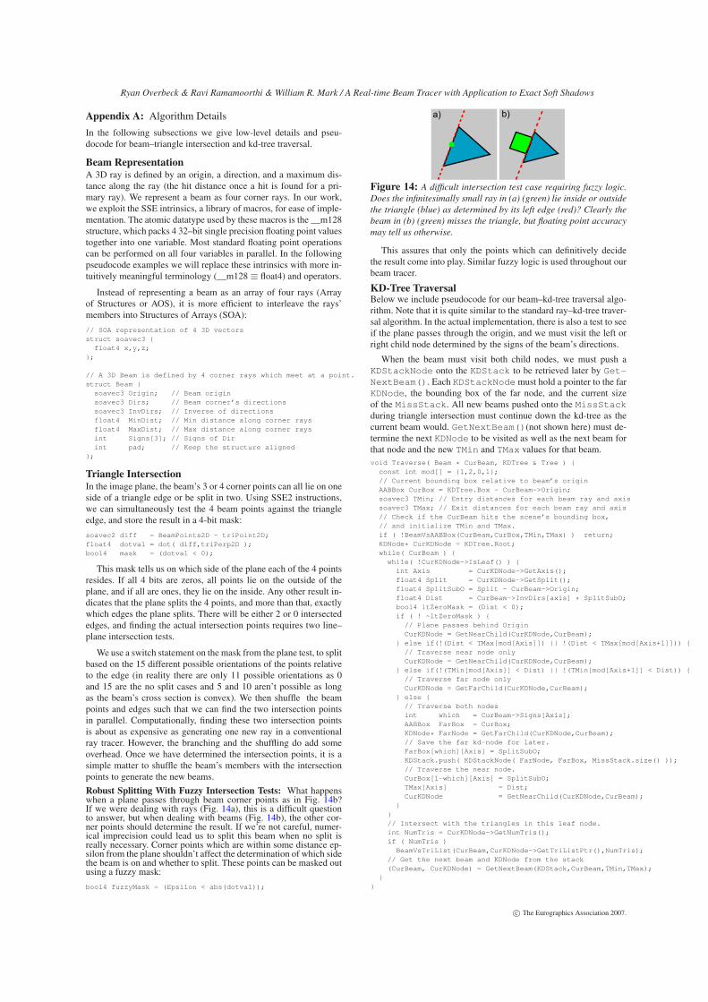
Robust Splitting With Fuzzy Intersection Tests: What happenswhen a plane passes through beam corner points as in Fig. 14b?If we were dealing with rays (Fig. 14a), this is a difficult questionto answer, but when dealing with beams (Fig. 14b), the other cor-ner points should determine the result. If we’re not careful, numer-ical imprecision could lead us to split this beam when no split isreally necessary. Corner points which are within some distance ep-silon from the plane shouldn’t affect the determination of which sidethe beam is on and whether to split. These points can be masked outusing a fuzzy mask:

bool4 fuzzyMask = (Epsilon < abs(dotval));

a) b)

Figure 14: A difficult intersection test case requiring fuzzy logic.

Does the infinitesimally small ray in (a) (green) lie inside or outside

the triangle (blue) as determined by its left edge (red)? Clearly the

beam in (b) (green) misses the triangle, but floating point accuracy

may tell us otherwise.

This assures that only the points which can definitively decidethe result come into play. Similar fuzzy logic is used throughout ourbeam tracer.

KD-Tree TraversalBelow we include pseudocode for our beam–kd-tree traversal algo-rithm. Note that it is quite similar to the standard ray–kd-tree traver-sal algorithm. In the actual implementation, there is also a test to seeif the plane passes through the origin, and we must visit the left orright child node determined by the signs of the beam’s directions.

When the beam must visit both child nodes, we must push aKDStackNode onto the KDStack to be retrieved later by Get-NextBeam(). Each KDStackNode must hold a pointer to the farKDNode, the bounding box of the far node, and the current sizeof the MissStack. All new beams pushed onto the MissStackduring triangle intersection must continue down the kd-tree as thecurrent beam would. GetNextBeam()(not shown here) must de-termine the next KDNode to be visited as well as the next beam forthat node and the new TMin and TMax values for that beam.void Traverse( Beam * CurBeam, KDTree & Tree ) {

const int mod[] = {1,2,0,1};

// Current bounding box relative to beam’s origin

AABBox CurBox = KDTree.Box - CurBeam->Origin;

soavec3 TMin; // Entry distances for each beam ray and axis

soavec3 TMax; // Exit distances for each beam ray and axis

// Check if the CurBeam hits the scene’s bounding box,

// and initialize TMin and TMax.

if ( !BeamVsAABBox(CurBeam,CurBox,TMin,TMax) ) return;

KDNode* CurKDNode = KDTree.Root;

while( CurBeam ) {

while( !CurKDNode->IsLeaf() ) {

int Axis = CurKDNode->GetAxis();

float4 Split = CurKDNode->GetSplit();

float4 SplitSubO = Split - CurBeam->Origin;

float4 Dist = CurBeam->InvDirs[axis] * SplitSubO;

bool4 ltZeroMask = (Dist < 0);

if ( ! ~ltZeroMask ) {

// Plane passes behind Origin

CurKDNode = GetNearChild(CurKDNode,CurBeam);

} else if(!(Dist < TMax[mod[Axis]]) || !(Dist < TMax[mod[Axis+1]])) {

// Traverse near node only


} else if(!(TMin[mod[Axis]] < Dist) || !(TMin[mod[Axis+1]] < Dist)) {

// Traverse far node only

CurKDNode = GetFarChild(CurKDNode,CurBeam);

} else {

// Traverse both nodes

int which = CurBeam->Signs[Axis];

AABBox FarBox = CurBox;

KDNode* FarNode = GetFarChild(CurKDNode,CurBeam);

// Save the far kd-node for later.

FarBox[which][Axis] = SplitSubO;

KDStack.push( KDStackNode( FarNode, FarBox, MissStack.size() ));

// Traverse the near node.

CurBox[1-which][Axis] = SplitSubO;

TMax[Axis] = Dist;


}

}

// Intersect with the triangles in this leaf node.

int NumTris = CurKDNode->GetNumTris();

if ( NumTris )

BeamVsTriList(CurBeam,CurKDNode->GetTriListPtr(),NumTris);

// Get the next beam and KDNode from the stack

(CurBeam, CurKDNode) = GetNextBeam(KDStack,CurBeam,TMin,TMax);

}

}


a real-time beam tracer with application to exact soft shadows€¦ · · 2010-01-04a real-time...

Documents