a real time dosimetric system using cmos sensors for ... · for absorption is smaller than that for...
TRANSCRIPT

A Real Time Dosimetric System using CMOS Sensors for Secondary Neutrons
in Radiotherapy
Nicolas Arbor (IPHC – Strasbourg) Jean-Michel Létang (CREATIS – Lyon)
Journée PEPS FaiDoRa 2016 Paris – 06 Mars 2017
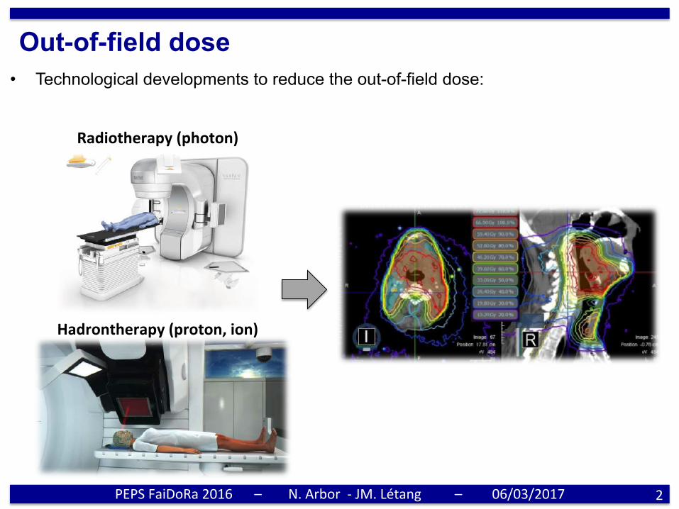
Out-of-field dose • Technological developments to reduce the out-of-field dose:
PEPSFaiDoRa2016 – N.Arbor-JM.Létang – 06/03/2017 2
Radiotherapy(photon)
Hadrontherapy(proton,ion)
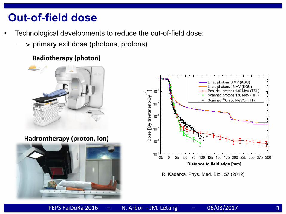
Out-of-field dose • Technological developments to reduce the out-of-field dose:
primary exit dose (photons, protons)
PEPSFaiDoRa2016 – N.Arbor-JM.Létang – 06/03/2017 3
Out-of-field dose measurements in a water phantom 5067
Figure 6. Overview of the lateral dose profiles measured for all radiation types and deliverytechniques. The measurements were obtained with the diamond detector in the depth of maximumdose (15 mm for 6 MV photons, 31 mm for 18 MV photons and 125 mm for protons and carbonions) during an irradiation with a 5 × 5 cm2 field.
account. In fact, irradiations with smaller fields correspond to a higher number of primary ionsstopped in the collimator and thus a larger yield of secondary neutrons. For scanned protonsa slight increase of the out-of-field dose far from the target is observed at increasing field size.The higher number of primary protons necessary to produce a larger homogeneous field withthe scanning technique is translated into a higher number of scattered protons which deposittheir energy outside the target.
Unlike protons, the dependence of the lateral dose distribution on the field size is verystrong for carbon ions. A larger field size is translated into an increase of the out-of-field doseby up to one order of magnitude. This behavior is the direct consequence of the increasingyield of secondary particles produced through nuclear fragmentation with increasing numberof primary ions required to irradiate a larger field. The irregular trend in the region up to 50 mmfrom the field edge is due to the fact that the experiment was not performed in the medicalcave of GSI; therefore, the beam tuning quality was not as high as for the other measurements.
Finally, the behavior of the lateral dose profile for different delivery modalities wasinvestigated. The comparison between passively delivered and scanned protons for a givenfield size (5 × 5 cm2) is shown in figures 5 (a) and (b). The beam shaped with passive elementsis characterized by a sharper penumbra because of the presence of the collimator close tothe water phantom which stops the primary protons scattered outside the field. At largerdistances from the region directly irradiated (above 100 mm), the dose profile of the passivelymodulated beam flattens at around 2 × 10⁻⁴ Gy·treatment-Gy−1 and stays rather constant upto 200 mm from the field edge, while the dose curve of the scanned beam drops sharply below10−5 Gy·treatment-Gy−1.
The overview and comparison of the results collected with the diamond detector are shownin figure 6 for 6 and 18 MV photons and ions of 125 mm range in water.
Independent of the radiation type and delivery technique, the lateral dose drops downto 10% of the target dose within 10 mm from the field edge; however, at increasing lateraldistances the values for photons are a factor of 50–400 higher than that for charged particles
R. Kaderka, Phys. Med. Biol. 57 (2012)
Radiotherapy(photon)
Hadrontherapy(proton,ion)

Out-of-field dose • Technological developments to reduce the out-of-field dose:
primary exit dose (photons, protons) secondary dose (photons, neutrons, ions)
⇒ irradiation far away from the tumor (whole treatment room) ⇒ low dose region (less than 1% of the total dose)...but not without risks
4
Phys. Med. Biol. 59 (2014) 2457 R A Halg et al
−10 0 10 20 30 40 50 60 70 80Distance along patient axis x/cm
10−3
10−2
10−1
100
Neu
tron
dos
eeq
uiv
alen
tH
/mSv/
trea
tmen
tG
y
Varian IMRT TPR20,10 = 0.760
Elekta IMRT TPR20,10 = 0.757
Siemens IMRT TPR20,10 = 0.773
Figure 4. Neutron dose equivalent along the medial patient axis. The isocentercorresponds to x = 0 cm and the vertical lines represent the border of the targetvolume along this axis. IMRT treatments on different linear accelerators. The error barsrepresent a standard uncertainty of 28%.
−10 0 10 20 30 40 50 60 70 80Distance along patient axis x/cm
10−3
10−2
10−1
100
101
Neu
tron
dos
eeq
uiv
alen
tH
/mSv/
trea
tmen
tG
y
Active protons PSI
Passive protons MGH
Varian IMRT
Figure 5. Neutron dose equivalent along the medial patient axis. The isocentercorresponds to x = 0 cm and the vertical lines represent the border of the targetvolume along this axis. Active and passive proton therapy compared to photon IMRTon the Varian linear accelerator. The error bars represent a standard uncertainty of 28%.
4. Discussion
The observed differences in neutron dose equivalent between the different treatment techniqueson the Varian linear accelerator were within the measurement uncertainty for most of themeasurement points. The 3DCRT treatment tends to have lower neutron dose equivalentoutside of the primary field close to the field border but higher dose within the treatment field.This finding is consistent with another study by Halg et al where the neutron dose equivalentsfrom open and intensity-modulated fields in a geometrical phantom were compared (Halg et al2012).
For high energy photon beams, the neutrons are mostly produced in the gantry head(McCall et al 1984). The amount of neutrons produced in the patient (materials with lowatomic number Z) is about a factor of 10 (Ongaro et al 2000) to 50 (Zanini et al 2004) lower
2463
R.A. Hälg, Phys. Med. Biol. 59 (2014)
PEPSFaiDoRa2016 – N.Arbor-JM.Létang – 06/03/2017
J. Farah, Phys. Med. Biol. 59 (2014)
Phys. Med. Biol. 59 (2014) 2747 J Farah et al
Figure 5. H∗(10) cartography inside the 75 MeV (left) and the 178 MeV treatmentrooms (right).
Table 2. Comparison of H∗(10) measurements with the Berthold, Wendi-2 and Hawkcounters.
75 MeV 178 MeV
Measurement Berthold) Wendi-2 Hawk Berthold Wendi-2 Hawkpoint (µSv.Gy−1) (µSv.Gy−1) (µSv.Gy−1) (µSv.Gy−1) (µSv.Gy−1) (µSv.Gy−1)
1 26 23 30 185 195 1652 13 13 16 110 129 1103 7 8 7 – 335 –4 4 4 3 – 155 –5 12 13 14 230 255 241
while neutrons <50 keV only deposit 5% of the dose. At this energy range, the Berthold,Wendi-2 and Hawk have a similar response, provided they are calibrated at the same energyrange. In addition, the highest H
∗(10) levels were measured at the closest distances to the beam
line and for angles !90◦; namely position #1 for the 75 MeV and position #3 for the 178 MeV.This is mainly due to the fact that neutrons with the lowest energies are emitted with highangular deviations with respect to the beam line. The observation of an H
∗(10) maximum at
such close positions could also be due to the contribution of secondary protons interacting inthe detectors or moderators (Trompier et al 2007). In addition, measured H
∗(10) values show a
symmetrical distribution of neutrons around the beam line element since similar ambient doseequivalent values were registered at points 2 and 5 located at ± 90◦ alongside the isocenter forthe 75 MeV proton beam. Finally, and although H∗(10) measurement positions were fartherfor the 178 MeV beam when compared to the 75 MeV beam, the H
∗(10) values were up to
∼100 times higher for the highest energy beam. This observation was expected since neutrongeneration is directly proportional to the proton beam energy. H∗(10) cartography (normalizedto the proton dose (D) delivered to the SOBP plateau) within the treatment room was alsosimulated in MCNPX. Figure 5 shows the simulation results which indicate that the maingenerators of secondary neutrons are found at the level of the beam line elements (red color).
Next, simulated H∗(10) values were compared to the mean values measured by the three
instruments (cf figures 6(a) and (b)). Both measured and calculated H∗(10) were normalized to
the proton dose (DT) delivered to the SOBP plateau. Again simulations showed that H∗(10)/DT
values decrease as the distance to the isocenter increases and as the angular direction (θ )
2757
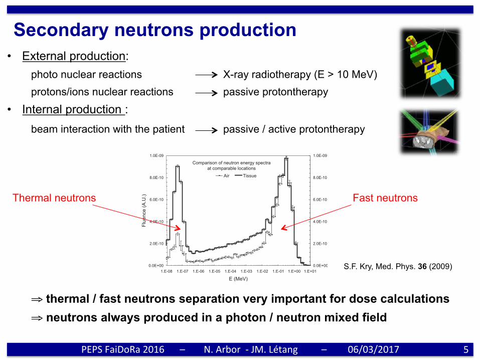
Secondary neutrons production • External production:
photo nuclear reactions X-ray radiotherapy (E > 10 MeV) protons/ions nuclear reactions passive protontherapy
• Internal production : beam interaction with the patient passive / active protontherapy
⇒ thermal / fast neutrons separation very important for dose calculations ⇒ neutrons always produced in a photon / neutron mixed field
5Hn+n!
= Qeff!Dn + Dn!" = Qn · Dn + Dn!
, !3"
where Hn+n! is the dose equivalent from neutrons and cap-ture gammas, Dn is the dose from neutrons and Dn! is thedose from capture gammas !which have a defined qualityfactor of 1".23 Use of Qeff is confounded by its dependenceon the geometry of the patient and radiation field, as theseparameters affect the relative importance of photons and neu-trons. That is, while Qn depends only on the neutron energyspectrum and the material composition of the medium inwhich those neutrons interact, Qeff depends additionally onthe size and shape of the phantom or patient and the direc-tionality of the radiation field and is therefore difficult todefine uniquely. Qeff is most commonly considered in thecontext of the effective dose equivalent for a person, HE,which, when divided by the organ-weighted absorbed physi-cal dose D!, yields the specially defined Qeff of qE:
HE
D!= qE. !4"
The value of qE is of general interest because it is after thisvalue that the most recent radiation weighting factors wRhave been patterned !although they are different by a scalingfactor".23 Numerically, the values of Qn and qE or wR aresimilar but are most distinct for thermal neutrons, where Qnis 16.2 !in tissue"22 while qE and wR are around 2.23
III. RESULTS
Figure 2 shows the neutron fluence with the phantompresent and absent. With the phantom absent !“air”", the totalneutron fluence decreased with distance in an approximatelyinverse square manner. The presence of the phantom drasti-cally affected the neutron fluence as neutrons are readilyscattered. The presence of the full-sized phantom thereforeproduces a full-scatter scenario, analogous to full phantomscatter in photon beams. There was a marked increase in theneutron fluence near the surface of the phantom and in the airup to 20 cm above the phantom. The neutron fluence reached
a maximum at approximately 2 cm depth in the phantom,beyond which it decreased sharply with depth.
Figure 3 compares neutron spectra in air and at a 0.1 cmdepth in tissue, calculated at the same location: 25 cm awayfrom the central axis. Error bars based on the statistical un-certainty are included for both spectra and are relativelysmall. Both spectra showed a predominance of neutronsaround 0.4 MeV that were primarily direct neutrons, that is,neutrons that traveled directly from the accelerator head tothe patient. At energies below this peak, the spectra alsoshowed the presence of epithermal neutrons, which were pri-marily scattered neutrons, that is, neutrons that scatteredthroughout the treatment vault. Finally, at energies of10−7–10−8 MeV, both spectra showed a peak of thermalneutrons that originated largely from neutron interactionswith hydrogen !either in tissue or in the concrete of the treat-ment vault". Although both spectra were calculated at thesame position relative to the isocenter, the increased scatterfrom the phantom resulted in an increase in total fluencefrom 116"103 to 192"103 n /cm2 /MU with the presenceof the phantom, with a small statistical uncertainty of lessthan 1% in each value. There was also a decrease in theaverage neutron energy from 0.24 MeV in air to 0.14 MeV intissue, with statistical uncertainties of 1.6% and 1.3%, re-spectively, in these values.
Figure 4 shows the neutron spectra in tissue at depthsfrom 0.1 to 19.5 cm. At shallow depths !0.1–4.5 cm", therewas a substantial decrease in the direct neutron peak at 0.4MeV and an increase in the thermal neutron peak at10−7–10−8 MeV with increasing depth. These changes oc-curred as fast neutrons lose energy and rapidly become ther-malized, primarily because they have a relatively large crosssection for elastic scatter with hydrogen.1 The buildup ofthermal neutrons occurred because the neutron cross sectionsare different for elastic scatter and neutron capture. Neutronabsorption occurs only with thermal neutrons !primarilythrough absorption by nitrogen"; however, the cross sectionfor absorption is smaller than that for elastic scattering. Atdepths deeper than 4.5 cm, an increase in depth in tissue
Comparison of neutron fluence as a function of depthin tissue (phantom present) and air (phantom absent)
0.E+00
1.E-08
2.E-08
3.E-08
4.E-08
-30 -20 -10 0 10 20 30
Depth (cm)
Fluence(A.U.)
0.E+00
1.E-08
2.E-08
3.E-08
4.E-08
Tissue Air
FIG. 2. Neutron fluence in arbitrary units !A.U." as a function of depth intissue !d" with the phantom present or absent. Phantom surface was locatedat d=0 and negative depths refer to the fluence in air above the phantom.
Comparison of neutron energy spectraat comparable locations
0.0E+00
2.0E-10
4.0E-10
6.0E-10
8.0E-10
1.0E-09
1.E-08 1.E-07 1.E-06 1.E-05 1.E-04 1.E-03 1.E-02 1.E-01 1.E+00 1.E+01
E (MeV)
Fluence(A.U.)
0.0E+00
2.0E-10
4.0E-10
6.0E-10
8.0E-10
1.0E-09
Air Tissue
FIG. 3. Neutron energy spectra in A.U. from a Varian 2100 accelerator cal-culated at the same location relative to the treatment head in air and at 0.1cm depth in tissue.
1246 Kry et al.: Neutron dose equivalents in tissue 1246
Medical Physics, Vol. 36, No. 4, April 2009
S.F. Kry, Med. Phys. 36 (2009)
PEPSFaiDoRa2016 – N.Arbor-JM.Létang – 06/03/2017
Fast neutrons Thermal neutrons
Neutron measurements • Neutrons production depends on various parameters :
- room and accelerator design - beam (energy, field size, angle, ...) - patient (irradiated volume, morphology, ...)
⇒ large disparity of available neutron dosimetric data
6
oneneutronphasespaceforeachtreatment(inaspecificfacility)
PEPSFaiDoRa2016 – N.Arbor-JM.Létang – 06/03/2017

Neutron measurements • Neutrons production depends on various parameters :
- room and accelerator design - beam (energy, field size, angle, ...) - patient (irradiated volume, morphology, ...)
⇒ large disparity of available neutron dosimetric data
• Most widely used detectors : solid nuclear track detector (SNTD)
⇒ new detector development to expand (simplify) neutron monitoring
7
oneneutronphasespaceforeachtreatment(inaspecificfacility)
23/09/2016 Halima Elazhar
16
Neutron detectors
Oxide layer ≈ 7 μm Epitaxial layer ≈ 14 μm
Bulk
2.5 mm
Original surface
Post-etched surface
9Neutron detected through the damage trails created by recoil nuclei of the converters
9Complementary Metal Oxyde Semi-Conductor
Passive detector
Solide State Nuclear Track Detectors (CR-39)
Real-time detector
CMOS sensor (AlphaRad)
CR-39
✓ gammatransparent✓smallsize(inphantommeasurements)✗thermal/fastneutronsseparaPon(internaldosemeasurements)✗calibraPon(tracksódose)dependentonneutronspectrum✗chemicaletching(Pmeconsuming,noreuse)
PEPSFaiDoRa2016 – N.Arbor-JM.Létang – 06/03/2017

Neutron detection
8PEPSFaiDoRa2016 – N.Arbor-JM.Létang – 06/03/2017
• Fast neutrons n+H à n + p Hydrogenated converters (CH2)n
• Thermal neutrons
n+10Bà α + 7Li Boron converters
Fast n
Converter (CH2)n
Detector
thermal n
Converter 10B
Detector
p
α
Thermal Fast Intermediate 0,01 eV 0,5 eV 200 keV 10 MeV
Relativist
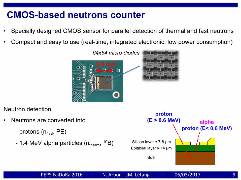
CMOS-based neutrons counter • Specially designed CMOS sensor for parallel detection of thermal and fast neutrons
• Compact and easy to use (real-time, integrated electronic, low power consumption)
Neutron detection
• Neutrons are converted into :
- protons (nfast, PE)
- 1.4 MeV alpha particles (ntherm, 10B)
9
2.5 mm
Silicon layer ≈ 7-8 µm Epitaxial layer ≈ 14 µm
Bulk
alpha proton (E< 0.6 MeV)
proton (E > 0.6 MeV)
64x64 micro-diodes
PEPSFaiDoRa2016 – N.Arbor-JM.Létang – 06/03/2017

CMOS-based neutrons counter • Specially designed CMOS sensor for parallel detection of thermal and fast neutrons
• Compact and easy to use (real-time, integrated electronic, low power consumption)
Neutron detection
• Neutrons are converted into :
- protons (nfast, PE)
- 1.4 MeV alpha particles (ntherm, 10B)
• Maximum proton energy loss Eloss ≈ 1 MeV
10
2.5 mm
Silicon layer ≈ 7-8 µm Epitaxial layer ≈ 14 µm
Bulk
64x64 micro-diodes
Eloss[MeV]1 1.4
protonalpha
amplitudegap⇒ parPcleidenPficaPon
PEPSFaiDoRa2016 – N.Arbor-JM.Létang – 06/03/2017
Energy loss [keV]0 200 400 600 800 1000 1200 1400
N
-310
-210
-110
Particle type
Gamma (Geant4)
Proton (Geant4)
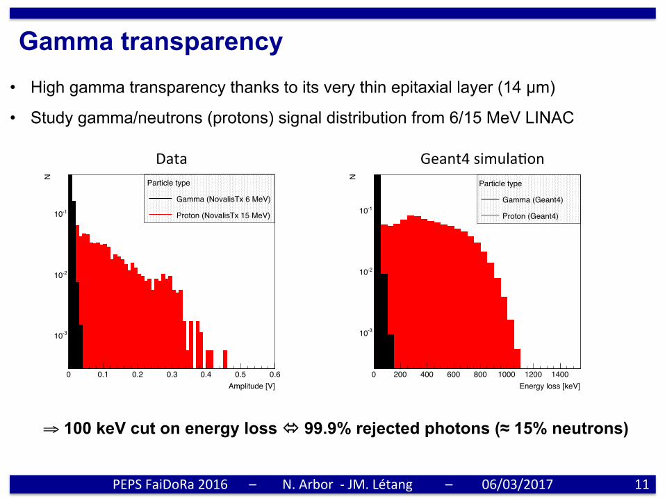
Gamma transparency • High gamma transparency thanks to its very thin epitaxial layer (14 µm)
• Study gamma/neutrons (protons) signal distribution from 6/15 MeV LINAC
⇒ 100 keV cut on energy loss ó 99.9% rejected photons (≈ 15% neutrons)
11
Amplitude [V]0 0.1 0.2 0.3 0.4 0.5 0.6
N
-310
-210
-110
Particle type
Gamma (NovalisTx 6 MeV)
Proton (NovalisTx 15 MeV)
Data Geant4simulaPon
PEPSFaiDoRa2016 – N.Arbor-JM.Létang – 06/03/2017
Energy [MeV]0 10 20 30 40 50 60
N /
(65
MeV
pro
ton)
-910
-810
-710
-610
-510
-410
-310
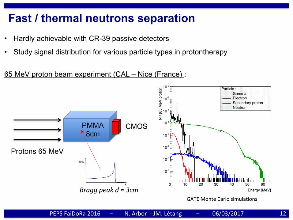
-210 Particle :GammaElectronSecondary protonNeutron
Fast / thermal neutrons separation • Hardly achievable with CR-39 passive detectors
• Study signal distribution for various particle types in protontherapy
12
Protons 65 MeV
PMMA 8cm
CMOS
GATEMonteCarlosimulaPonsBraggpeakd≈3cm
65 MeV proton beam experiment (CAL – Nice (France) :
PEPSFaiDoRa2016 – N.Arbor-JM.Létang – 06/03/2017
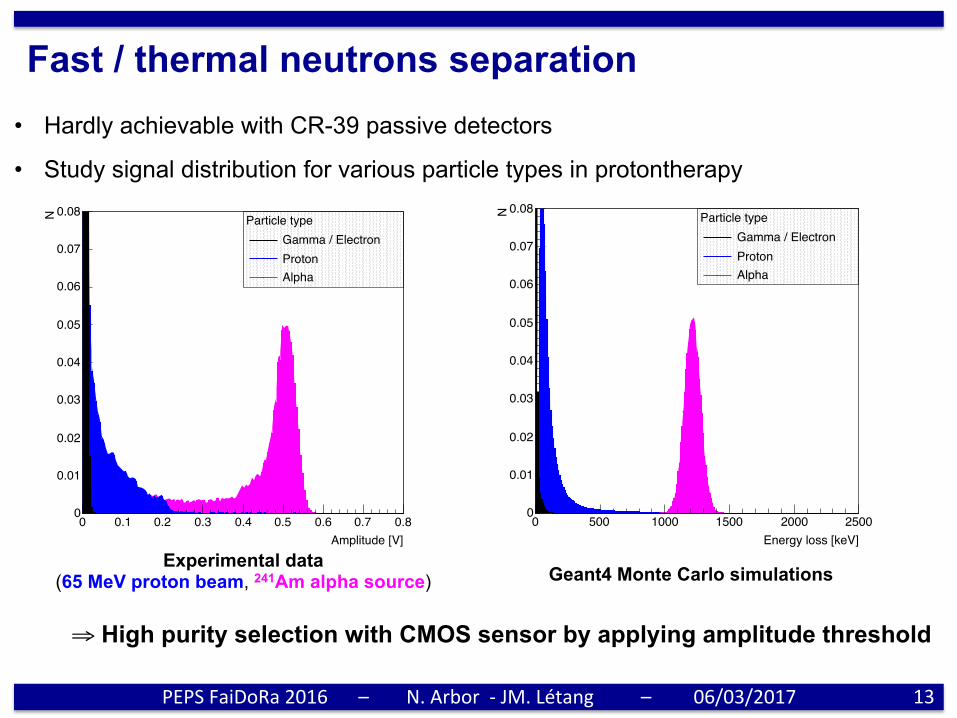
Energy loss [keV]0 500 1000 1500 2000 2500
N0
0.01
0.02
0.03
0.04
0.05
0.06
0.07
0.08Particle type
Gamma / ElectronProtonAlpha
Amplitude [V]0 0.1 0.2 0.3 0.4 0.5 0.6 0.7 0.8
N
0
0.01
0.02
0.03
0.04
0.05
0.06
0.07
0.08Particle type
Gamma / ElectronProtonAlpha
Geant4 Monte Carlo simulations Experimental data
(65 MeV proton beam, 241Am alpha source)
Fast / thermal neutrons separation • Hardly achievable with CR-39 passive detectors
• Study signal distribution for various particle types in protontherapy
13
⇒ High purity selection with CMOS sensor by applying amplitude threshold
PEPSFaiDoRa2016 – N.Arbor-JM.Létang – 06/03/2017

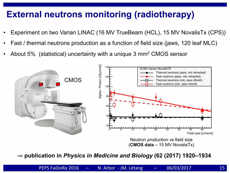
External neutrons monitoring (radiotherapy)
• Experiment on two Varian LINAC (16 MV TrueBeam (HCL), 15 MV NovalisTx (CPS))
• Fast / thermal neutrons production as a function of field size (jaws, 120 leaf MLC)
14PEPSFaiDoRa2016 – N.Arbor-JM.Létang – 06/03/2017
External neutrons monitoring (radiotherapy)
• Experiment on two Varian LINAC (16 MV TrueBeam (HCL), 15 MV NovalisTx (CPS))
• Fast / thermal neutrons production as a function of field size (jaws, 120 leaf MLC)
• About 5% (statistical) uncertainty with a unique 3 mm2 CMOS sensor
15
CMOS
PEPSFaiDoRa2016 – N.Arbor-JM.Létang – 06/03/2017
Neutron production vs field size (CMOS data – 15 MV NovalisTx)
Field size [cmxcm]0 5 10 15 20 25 30 35 40
Alph
a / P
roto
n [/G
y/cm
2]
20
40
60
80
100
120
14016 MV Varian TrueBeam
Thermal neutrons (jaws, mlc retracted)
Fast neutrons (jaws, mlc retracted)
Field size [cmxcm]0 5 10 15 20 25 30 35 40
Alph
a / P
roto
n [/G
y/cm
2]
20
40
60
80
100
120
140 15 MV Varian NovalisTXThermal neutrons (jaws, mlc retracted)Fast neutrons (jaws, mlc retracted)Thermal neutrons (mlc, jaws 40x40)Fast neutrons (mlc, jaws 40x40)
⇒ publication in Physics in Medicine and Biology (62 (2017) 1920–1934
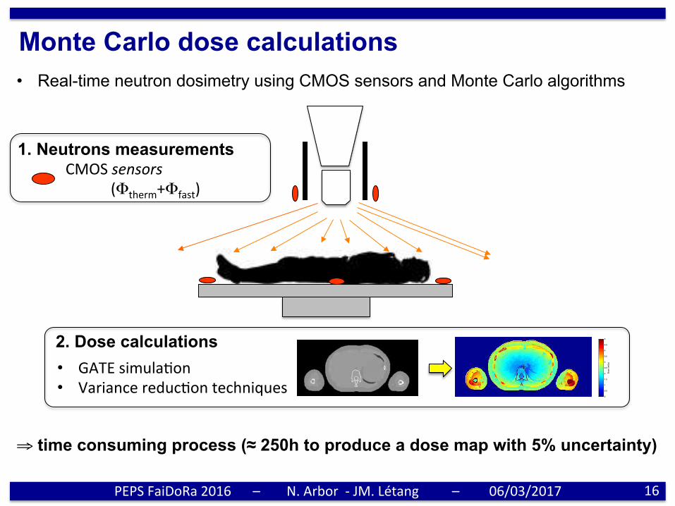
Monte Carlo dose calculations • Real-time neutron dosimetry using CMOS sensors and Monte Carlo algorithms
CMOSsensors (Φtherm+Φfast)
1. Neutrons measurements
ranges. The results were compared to the predictions of the reference plan based on the true ICRP materialscomposition. The comparison showed that range uncertainties introduced by wrong material compositions arenot significant compared to the above-described range uncertainty of 0.05 mm. This result validated the use ofwater equivalent materials for proton range calculations in this analysis framework.
3 Results
3.1 Calibration
Calibration curves obtained with X-ray and proton CT scanner simulations of a Gammex 467 phantom canbe observed in Figure 5. The curves have been produced from the mean value and the standard deviation ofeach insert computed in a circular region (2 cm diameter) slightly smaller than the insert size to avoid bordereffects. For soft tissue inserts with a Hounsfield Unit (HU) value around 0, some inserts with similar HU valuehave a quite different RSP.
Reconstructed values from X-ray CT have been both linearly interpolated (Figure 5, left) and fitted withtwo linear functions in a least-squares minimization (Figure 5, middle). Reconstructed values from the protonCT (Figure 5, right) have been adjusted with a unique linear function close to identity which was therefore notused in the following.
HU (X-ray CT)
-500 0 500 1000 1500
RS
P
0
0.2
0.4
0.6
0.8
1
1.2
1.4
1.6
1.8
HU (X-ray CT)
-500 0 500 1000 1500
RS
P
0
0.2
0.4
0.6
0.8
1
1.2
1.4
1.6
1.8
RSP (proton CT)
0.2 0.4 0.6 0.8 1 1.2 1.4 1.6
RS
P
0.2
0.4
0.6
0.8
1
1.2
1.4
1.6
1.8
0.014± 0.013 + x*1.006 ±y = -0.001
Figure 5: Calibration curves for X-ray and proton CT scanner simulations of a Gammex 467 phantom. For theX-ray CT, reconstructed values are linearly interpolated (left) or fitted with two linear functions (middle). Forthe proton CT, reconstructed values are fitted with a unique linear function (right).
3.2 Imaging dose
The dose maps of each site and each modality are provided in Figure 6 and the corresponding DoseVolume-Histograms (DVHs) in Figure 7. The DVHs have been computed in the full patient volume of about 220 litres.Large differences can be observed between the two maps with significantly more heterogeneity in the photondose maps and quite impressive uniformity in the proton dose maps. This translates into sharper DVHs forproton CT than X-ray CT, corresponding to a dose delivery more conformal to the imaged region. The dosecriterion, i.e., the same volume receiving 1 mGy or more in both modalities, is best visualized in Figure 7.
Do
se (
mG
y)
0
0.5
1
1.5
2
2.5
3
3.5
4
4.5
5
Figure 6: Spatial distribution of the dose delivered in proton (top) and X-ray (bottom) CT in mGy. For eachanatomical region (head, lungs and liver), coronal and axial slices at the isocenter (black cross) are provided.
6
2. Dose calculations • GATEsimulaPon • VariancereducPontechniques
ranges. The results were compared to the predictions of the reference plan based on the true ICRP materialscomposition. The comparison showed that range uncertainties introduced by wrong material compositions arenot significant compared to the above-described range uncertainty of 0.05 mm. This result validated the use ofwater equivalent materials for proton range calculations in this analysis framework.
3 Results
3.1 Calibration
Calibration curves obtained with X-ray and proton CT scanner simulations of a Gammex 467 phantom canbe observed in Figure 5. The curves have been produced from the mean value and the standard deviation ofeach insert computed in a circular region (2 cm diameter) slightly smaller than the insert size to avoid bordereffects. For soft tissue inserts with a Hounsfield Unit (HU) value around 0, some inserts with similar HU valuehave a quite different RSP.
Reconstructed values from X-ray CT have been both linearly interpolated (Figure 5, left) and fitted withtwo linear functions in a least-squares minimization (Figure 5, middle). Reconstructed values from the protonCT (Figure 5, right) have been adjusted with a unique linear function close to identity which was therefore notused in the following.
HU (X-ray CT)
-500 0 500 1000 1500
RS
P
0
0.2
0.4
0.6
0.8
1
1.2
1.4
1.6
1.8
HU (X-ray CT)
-500 0 500 1000 1500
RS
P
0
0.2
0.4
0.6
0.8
1
1.2
1.4
1.6
1.8
RSP (proton CT)
0.2 0.4 0.6 0.8 1 1.2 1.4 1.6
RS
P
0.2
0.4
0.6
0.8
1
1.2
1.4
1.6
1.8
0.014± 0.013 + x*1.006 ±y = -0.001
Figure 5: Calibration curves for X-ray and proton CT scanner simulations of a Gammex 467 phantom. For theX-ray CT, reconstructed values are linearly interpolated (left) or fitted with two linear functions (middle). Forthe proton CT, reconstructed values are fitted with a unique linear function (right).
3.2 Imaging dose
The dose maps of each site and each modality are provided in Figure 6 and the corresponding DoseVolume-Histograms (DVHs) in Figure 7. The DVHs have been computed in the full patient volume of about 220 litres.Large differences can be observed between the two maps with significantly more heterogeneity in the photondose maps and quite impressive uniformity in the proton dose maps. This translates into sharper DVHs forproton CT than X-ray CT, corresponding to a dose delivery more conformal to the imaged region. The dosecriterion, i.e., the same volume receiving 1 mGy or more in both modalities, is best visualized in Figure 7.
Do
se
(m
Gy
)
0
0.5
1
1.5
2
2.5
3
3.5
4
4.5
5
Figure 6: Spatial distribution of the dose delivered in proton (top) and X-ray (bottom) CT in mGy. For eachanatomical region (head, lungs and liver), coronal and axial slices at the isocenter (black cross) are provided.
6
0 0.5 1 1.5 2 2.5 30
1
2
3
4
5x 10
4
Dose (mGy)
Vo
lum
e (
cm3)
xCT HeadxCT LungxCT LiverpCT HeadpCT LungpCT Liver
Figure 7: Dose-volume histograms of the dose delivered in proton and X-ray CT for the three anatomical sites.
3.3 Relative stopping power maps
One slice of each RSP map is presented in Figure 8. A slight blurring of proton CT images due to multipleCoulomb scattering can still be observed, despite the use of a reconstruction algorithm accounting for the mostlikely path of protons (Rit et al. 2013).
(a) ICRP reference (b) Proton CT (c) X-ray CT (fit)
Figure 8: Example of reconstructed RSP maps for the head (top), lungs (middle) and liver (bottom) regions.Gray-level range: [0-1.708].
Voxel-by-voxel absolute deviation of the RSP has been computed for all RSP maps. The absolute deviationof the RSP is defined as the difference between reconstructed X-ray or proton CT RSP maps and the ICRPreference map. Results for the three sites have been combined in Figure 9.
Spatial uniformity of RSP deviation can also be observed in two dimensional image slices. The absolutedeviation between the X-ray and proton CT RSP maps and the ICRP reference were used to produce Figure 10.
3.4 Proton range
Proton ranges were estimated for the three anatomical sites. X-ray and proton CT based calculations havebeen compared to reference proton ranges. The absolute range deviation was computed beam-per-beam andtheir distribution has been summarized in Figure 11.
Using pencil beams with 120 mm range on average, the mean absolute deviation of the range predictionbased on X-ray CT varies from 0.18 to 2.01 mm while it is smaller than 0.1 mm for proton CT. Range standarddeviations are about 30% lower, and dispersion between sites are reduced from about 1 mm to less than 0.1mm. The comparison of the two X-ray CT calibration methods highlights smaller mean range deviations withthe linear interpolation but a larger dispersion between anatomical regions.
7
⇒ time consuming process (≈ 250h to produce a dose map with 5% uncertainty)
16PEPSFaiDoRa2016 – N.Arbor-JM.Létang – 06/03/2017
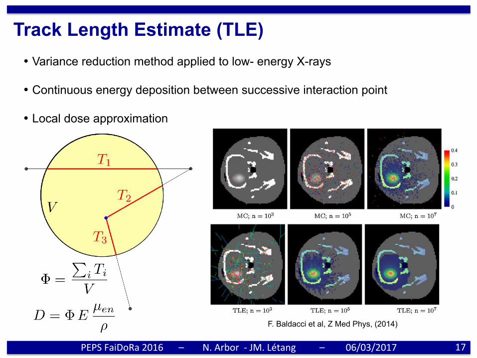
Track Length Estimate (TLE)
17 PEPSFaiDoRa2016 – N.Arbor-JM.Létang – 06/03/2017
• Variance reduction method applied to low- energy X-rays • Continuous energy deposition between successive interaction point • Local dose approximation
F. Baldacci et al, Z Med Phys, (2014)
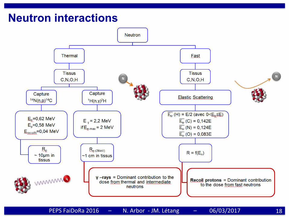
Neutron interactions
18 PEPSFaiDoRa2016 – N.Arbor-JM.Létang – 06/03/2017
Neutron TLE (nTLE)
19 PEPSFaiDoRa2016 – N.Arbor-JM.Létang – 06/03/2017
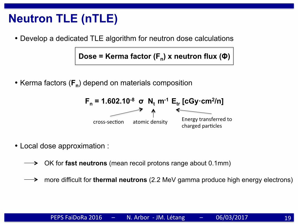
• Develop a dedicated TLE algorithm for neutron dose calculations
Dose = Kerma factor (Fn) x neutron flux (Φ)
• Kerma factors (Fn) depend on materials composition
Fn = 1.602.10-8 σ Nt m-1 Etr [cGy·cm2/n]
• Local dose approximation :
OK for fast neutrons (mean recoil protons range about 0.1mm) more difficult for thermal neutrons (2.2 MeV gamma produce high energy electrons)
cross-secPon atomicdensity EnergytransferredtochargedparPcles
20/01/2017 Halima Elazhar
7
9 Steady and good dose evaluation by NTLE for 1MeV neutrons 9 10 to 15 % dose overestimation respectively for thermal and 10 Mev neutrons => Next step : try to find a correction factor to lower dose overestimation
Single voxelised Raw after proper voxelisation
Dose Ratio : Raw of 1x1x10 mm3
In vacuum In middle of a cube
Dose and Variance reduction
20 PEPSFaiDoRa2016 – N.Arbor-JM.Létang – 06/03/2017
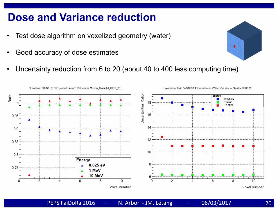
• Test dose algorithm on voxelized geometry (water) • Good accuracy of dose estimates • Uncertainty reduction from 6 to 20 (about 40 to 400 less computing time)
Heterogeneous materials
21 PEPSFaiDoRa2016 – N.Arbor-JM.Létang – 06/03/2017
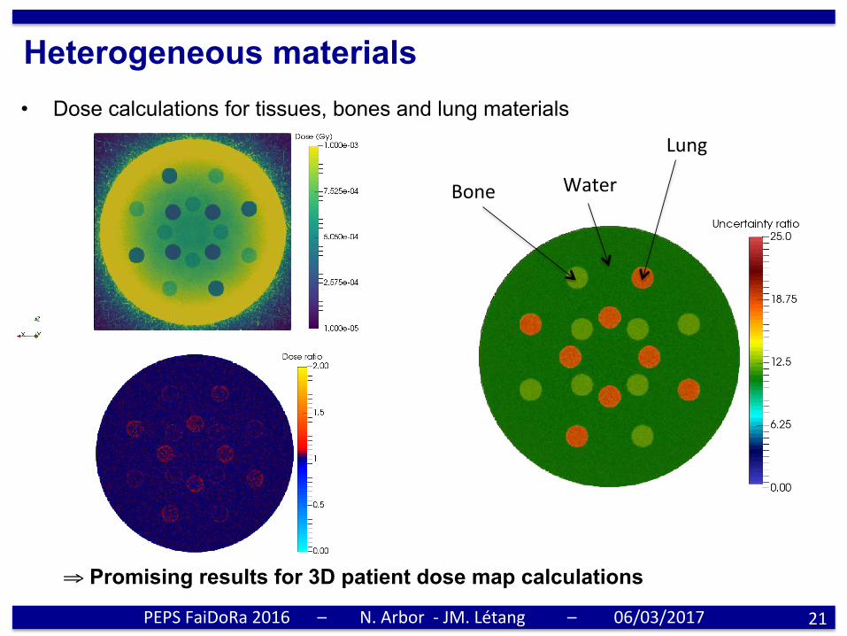
• Dose calculations for tissues, bones and lung materials
Lung
Water Bone
⇒ Promising results for 3D patient dose map calculations

Summary / Outlook
23
• Specially designed CMOS sensor for neutrons monitoring in radiotherapy • First application of CMOS based counter for external / internal neutrons production
high gamma transparency fast / thermal neutrons separation easy to use (real-time, compact, 3V battery, ...)
• Coupling with fast Monte Carlo dose algorithm for patient 3D dose maps • On-going system miniaturization (≈ 1 cm2) to realize in phantom measurements
Thanks for your attention
PEPSFaiDoRa2016 – N.Arbor-JM.Létang – 06/03/2017