A Recipe for Constructing A Recipe for Constructing a Peri-stimulus Time a Peri-stimulus Time

HistogramHistogram

Hideaki ShimazakiDept. of Physics Kyoto University, Japan

March 1, 2007 Johns Hopkins UniversityMarch 2, 2007 Columbia University

Peri-stimulus Time Peri-stimulus Time HistogramHistogram

Rep

eate

d t

rials

a PST Histograma PST Histogram

Events (Spikes)

From Spikes: Exploring the Neural Code, Rieke et al. 1997

George L. Gerstein and Nelson Y.-S. Kiang (1960 )An Approach to the Quantitative Analysis of Electrophysiological Data from Single Neurons, Biophys J. 1(1): 15–28.

Adrian, E. (1928). The basis of sensation: The action of the sense organs.

Prof. Gersteinme

Bin widthBin width@Kyoto Univ.

1. Bin Width Selection1. Bin Width SelectionUnknown

2ˆMISE t t dt Histogram

Underlying Rate

n 2

2k - vC (Δ) =

Δ

EstimateDatDataa

Method for Selecting the Bin Method for Selecting the Bin SizeSize

N

ii=1

1k k ,

N

N

2i

i=1

1v (k - k)

N

n 2

2k - vC (Δ) = ,

(nΔ)

• Compute the cost function

while changing the bin size Δ.

• Divide the data range into N bins of width Δ. Count the number of events ki in the i th bin.

4 2 1 4 3 1

Mean

Variance

• Find Δ* that minimize the cost function.

ik

n 2

2k - vC (Δ) =

(nΔ)n = 4

N = 6

Time-Varying Rate

Spike Sequences

Time Histogram

The spike count in the bin obeys the Poisson distribution*:

A histogram bar-height is an estimator of :

The mean underlying rate in an interval [0, ]:

0

1t dt

( )

k

nnp k n e

k

n̂

k

n

*When the spikes are obtained by repeating an independent trial, the accumulated data obeys the Poisson point process due to a general limit theorem.

Theory for the MethodTheory for the Method

22

0

1ˆMISE ( ) .n tE dt

2 2

0 0

1 1ˆ ˆMISE ( ) ( )T

t t n tE dt dtE

T

Expectation by the Poisson statistics, given the rate.

2 22

0 0

1 1t tdt dt

Variance of the rate Variance of

an ideal histogram

Decomposition of the Systematic Error

Systematic ErrorSampling Error

Average over segmented bins.

Independent of

Theory: Selection of the Bin SizeTheory: Selection of the Bin Size

Systematic Error

2

0

22

1( ) MISE

ˆ( )

T

n t

n

C dtT

E

22ˆ ˆ ˆ2n n n nC E E E

22 ˆ ˆ ˆn n n nC E E E

n

Variance of a Histogram

2 22ˆ ˆ ˆ( ) .n n nE E E

2 1ˆ ˆ( )n nE En

Introduction of the cost function:

The variance decomposition:

Mean of a Histogram

The Poisson statistics obeys:

Unknown: Variance of an ideal histogramSampling error

Variance of a histogram Sampling error

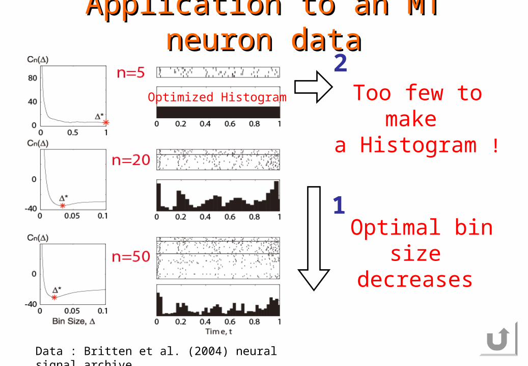
Data : Britten et al. (2004) neural signal archive

Application to an MT neuron Application to an MT neuron datadata

Too few to make

a Histogram !

Optimized Histogram

Optimal bin size decreases

1

2

Theories on the Optimal Bin Size

2

1 2 1 22 0 0

1

nCn

t t dt dtn

Theoretical cost function:Theoretical cost function:

Unknown

DatDataa

1 2t t Mean Correlation function

n 2

2k - vC (Δ) =

(nΔ)

Theory

Empirical

If you know the underlying rate, you can computeSee also Koyama and Shinomoto

J. Phys. A, 37(29):7255–7265. 2004

1 2 1 22 0 0

1nC t t dt dt

n

2 31 1( ) 0 0 0 ( )

3 12nC On

(i) Expansion of the cost function by :

1 3

6~

0 n

Scaling of the optimal bin size:

Theoretical cost function:

Number of sequence s, m

100

101

102

103

10-2

10-1

Scaling of the optimal bin size

-1/3

The expansion of the cost function by

When the number of sequences is large, the optimal bin size is very small

Ref. Scott (1979)

(ii) Divergence of the optimal bin size

2

2

1 1~ | |

1 1 1 1

n

c

C t dt t t dtn

un n

cn t dt

The expansion of the cost function by 1/

Critical number of trials:

cn n

cn n

Optimal bin size diverges.

Finite optimal bin size.

The second order phase transition.

Not all the process undergoes the first order phase transition. Others undergo the second order (discontinuous) phase transition.

When the number of sequences is small, the optimal bin size is very large.

n: small

n: large

nc: critical number of trials

Phase transitions of optimal Phase transitions of optimal bin sizebin size

*1

cn

1 5n 10n

15n

20n

25n

1 n

n: small

n: large

Back to Practice!

Data : Britten et al. (2004) neural signal archive

2. The extrapolation method2. The extrapolation method

Too few to make

a Histogram !

2

1 1( )m n

kC n C

m n n

Extrapolation

Estimation: At least 12 trials are

required.

Optimized Histogram

Verification of the extrapolation Verification of the extrapolation methodmethod

Extrapolated:

Finite optimal bin size

Original: Optimal bin size diverges

2

1 1( )m n

kC n C

m n n

( )nC

Required # of sequences (Estimation)

Optimal bin size v.s. m

Data Size UsedData Size Used # of sequences used

Required # of trials

cn

t dt

30

We have n=30 Sequneces

Data : Britten et al. (2004) neural signal archive

2. The extrapolation method2. The extrapolation method

Too few to make

a Histogram !

2

1 1( )m n

kC n C

m n n

Extrapolation

Estimation: At least 12 trials are

required.

Optimized Histogram

Advanced Topics

Line-Graph Time Histogram

( )

k

nnp k n e

k

01.t dt

2tL t

ˆ ˆ ˆ ˆˆ

2t tL

0

1t dt

A line-graph is constructed by connecting top-centers of adjacent bar-graphs.

An estimator of a line-graph

The spike count obeys the Poisson distribution

Rate

Spike Sequences

Time Histogram

^

^

t

Line-Graph Model

( )( ) ( ) ( 0) ( )

2

2 2 1( ) 2 2

3 ( ) 3 3nkCn

( ) ( )ik j( ) ( )ik j (0) ( )ik j ( ) ( )ik j

( ) ( )

1

( )n

p pi i

j

k k j

(i) Define the four spike counts,

{ 0 }p

( ) ( )

1

1 Np p

ii

kkN

( ) ( )( ) ( ) ( )

1

1 Np qp q p q

i ii

s k kk kN

( ) ( )( ) ( )( )

1 1

1 1( ) ( )

p qN np qp q i i

i ii j

k kk j k js

N n n n

( ) ( )( )

2 2( )

p q p qp q s s

n n

(ii) Summation of the spike count

Binned-average

Covariations w.r.t. bins

Bin-average of the covariation of spike count w.r.t. sequences,

(iv) Cost function:

(iii)

(v) Repatn i through iv by changing Δ. Find the optimal Δ that minimizes the cost function.

0 1 1 2 0 1

0 2 2 0 0 1

( ) ( )ik j

( ) ( )ik j

(0) ( )ik j

( ) ( ) 2 ( )i ik j t j

i

j

j

j

The covariances of an ideal line-graph model is

A Recipe for an optimal line-graph TH

The optimal Line-Graph The optimal Line-Graph HistogramHistogram

0.05 0.1 0.15 0.2 0.25 0.3

-100

-75

-50

-25

25

50

75

100

Line-Graph

Bar-Graph

The Line-graph histogram performs better if the rate is smooth.

Theoretical Cost Function

2

1 2 1 22 0 0

1

nCn

t t dt dtn

2

21 2 1 22 0 2

22 21

3n

tC t t dt dt

n

0

1 2 1 2 1 2 1 22 20 0 0

2 1

3 3t t dt dt t t dt dt

(Bar-Graph)

(Line-Graph)

2. Theories on the optimal 2. Theories on the optimal bin sizebin size

Generalization of Koyama and Shinomoto J. Phys. A, 37(29):7255–7265. 2004

2 31 1( ) 0 0 0 ( )

3 12nC On

1 3

6~

0 n

1 23

~(0 )n

3 4 52 37 181 49( ) 0 0 0 0 ( )

3 144 5760 2880nC On

1 5

1280~

181 0 n

1 296

~37 (0 )n

-0.3 -0.2 -0.1 0.1 0.2 0.3

20

40

60

80

100

-0.3 -0.2 -0.1 0.1 0.2 0.3

20

40

60

80

100

the second order term vanishes.

The expansion of the cost function by :

A smooth process: A correlation function is smooth at origin.

A jagged process: A correlation function has a cusp at origin.

(0 ) 0 (Bar-Graph)

(Line-Graph)

(Bar-Graph)

(Line-Graph)

(Bar-Graph)

(Line-Graph)

(0 ) 0

(i) Scalings of the optimal bin size

Identification of the scaling Identification of the scaling exponentsexponents

1 2~ n 1/ 2~ n

smooth

zig-zag

1 5~ n

smooth

zig-zag

1 3~ n smooth

zig-zag

Data Size UsedData Size Used Data Size UsedData Size Used

Bar-Graph HistogramLine-Graph Histogram

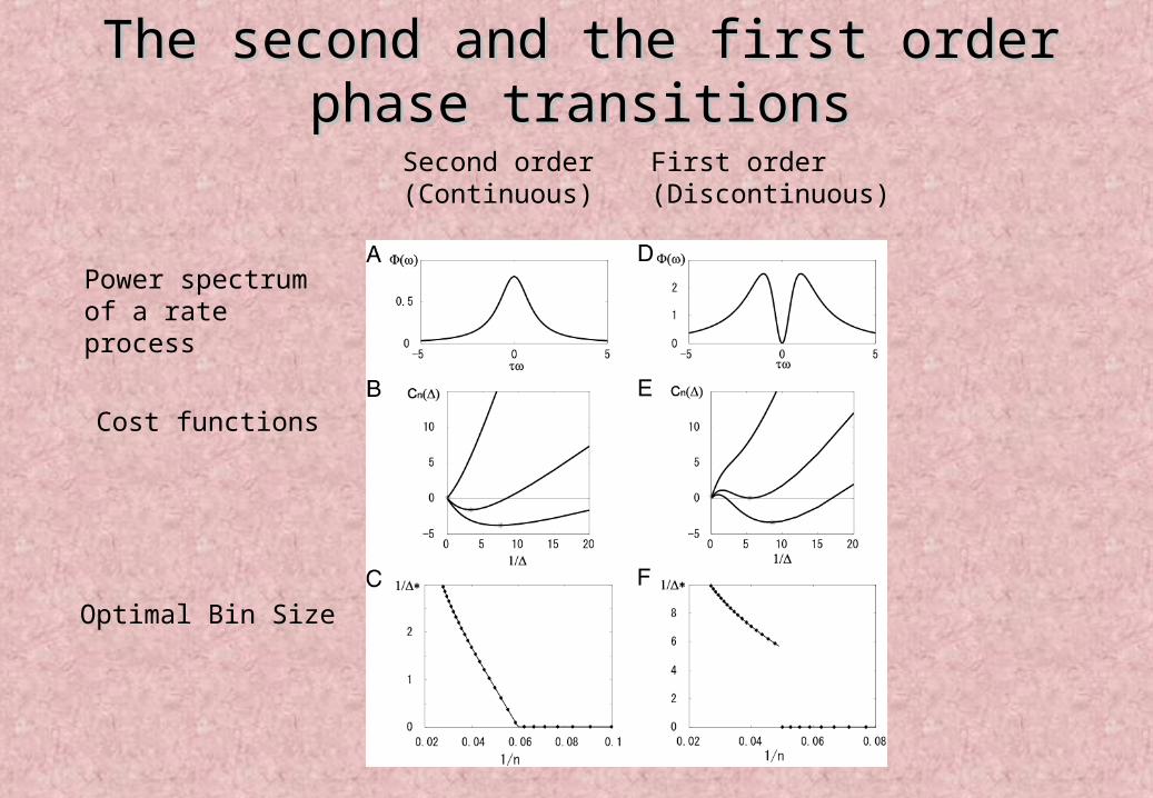
The second and the first order phase The second and the first order phase transitionstransitions

Power spectrum of a rate process

Cost functions

Optimal Bin Size

Second order(Continuous)

First order(Discontinuous)

Summary of Today’s Summary of Today’s TalkTalk

1. Bin width selection1. Bin width selection•The The methodmethod and and theorytheory

•Application to an MT neuronApplication to an MT neuron

2. Theories on the optimal bin width2. Theories on the optimal bin width•ScalingScaling and and Phase transitionsPhase transitions

3. Advice to experimentalists3. Advice to experimentalists•Extrapolation methodExtrapolation method

FAQ

N

2i

i=1

1v (k - k)

N2

2k - vC(Δ) =

Δ

too precise

Q. Can I apply the proposed method to a histogram for a probability distribution? A. Yes.

Q. I want to make a 2-dimensional histogram. Can I use this method? A. Yes.

Q. Can I use unbiased variance for computation of the cost function?A. No.

Q. I obtained a very small bin width, which is likely to be erroneous. Why?A. You probably searched smaller bin size than the sampling resolution.

Round Up

1

N

2i

i=1

1v (k - k)

N

Erroneously small optimal bin size

ReferenceReference

A Method for Selecting the Bin Size of a Time Histogram

Hideaki Shimazaki and Shigeru ShinomotoNeural Computation in Press

Short Summary: Adavances in Neural Information Processing Systems Vol. 19, 2007

• Web Application for the Bin Size Selection

• Matlab / Mathematica / R sample codes

are available at our homepagehttp://www.ton.scphys.kyoto-u.ac.jp/~shino/

/~hideaki/See alsoKoyama, S. and Shinomoto, S. Histogram bin width selection for time-dependent poisson processes. J. Phys. A, 37(29):7255–7265. 2004

AcknowledgementsAcknowledgements

JSPS Research Grant

Prof. Shigeru ShinomotoDr. Shinsuke Koyama

Hideaki Shimazaki

2007 Ph. D Prof. Shigeru Shinomoto

Dept. of Physics Kyoto University, Kyoto, Japan

2003 MA Prof. Ernst NieburDept. of Neuroscience, Johns Hopkins

University Baltimore, Maryland

2006-2008 JSPS Research Fellow

Introducing myself…

The Poisson Point The Poisson Point ProcessProcess

t

Pr One event in t

Pr More than one event in

t t

t O t

Samples are independently drawn from an identical distribution.

0

tt

Rate

Data