This is an author-deposited version published in : http://oatao.univ-toulouse.fr/ Eprints ID : 10259

To link to this article : DOI:10.1017/jfm.2011.363

URL : http://dx.doi.org/10.1017/jfm.2011.363

To cite this version : Magnaudet, Jacques A 'reciprocal' theorem for the prediction of loads on a body moving in an inhomogeneous flow at arbitrary Reynolds number. (2011) Journal of Fluid Mechanics, vol. 689 . pp. 564-604. ISSN 0022-1120

Any correspondence concerning this service should be sent to the repository administrator: staff-oatao@listes.diff.inp-toulouse.fr

brought to you by COREView metadata, citation and similar papers at core.ac.uk

provided by Open Archive Toulouse Archive Ouverte

A ‘reciprocal’ theorem for the prediction of loadson a body moving in an inhomogeneous flow at

arbitrary Reynolds number

Jacques Magnaudet†

Institut de Mecanique des Fluides de Toulouse, UMR CNRS/INPT/UPS 5502, Allee Camille Soula,31400 Toulouse, France

Several forms of a theorem providing general expressions for the force and torqueacting on a rigid body of arbitrary shape moving in an inhomogeneous incompressibleflow at arbitrary Reynolds number are derived. Inhomogeneity arises because ofthe presence of a wall that partially or entirely bounds the fluid domain and/or anon-uniform carrying flow. This theorem, which stems directly from Navier–Stokesequations and parallels the well-known Lorentz reciprocal theorem extensivelyemployed in low-Reynolds-number hydrodynamics, makes use of auxiliary solenoidalirrotational velocity fields and extends results previously derived by Quartapelle &Napolitano (AIAA J., vol. 21, 1983, pp. 911–913) and Howe (Q. J. Mech. Appl.Maths, vol. 48, 1995, pp. 401–426) in the case of an unbounded flow domain anda fluid at rest at infinity. As the orientation of the auxiliary velocity may be chosenarbitrarily, any component of the force and torque can be evaluated, irrespective ofits orientation with respect to the relative velocity between the body and fluid. Threemain forms of the theorem are successively derived. The first of these, given in (2.19),is suitable for a body moving in a fluid at rest in the presence of a wall. The mostgeneral form (3.6) extends it to the general situation of a body moving in an arbitrarynon-uniform flow. Specific attention is then paid to the case of an underlying time-dependent linear flow. Specialized forms of the theorem are provided in this situationfor simplified body shapes and flow conditions, in (3.14) and (3.15), making explicitthe various couplings between the body’s translation and rotation and the strain rateand vorticity of the carrying flow. The physical meaning of the various contributionsto the force and torque and the way in which the present predictions reduce tothose provided by available approaches, especially in the inviscid limit, are discussed.Some applications to high-Reynolds-number bubble dynamics, which provide severalapparently new predictions, are also presented.

Key words: general fluid dynamics, vortex dynamics

1. IntroductionGiven its many applications in all sorts of domains (e.g. oceanography, meteorology,

flight dynamics, and mechanical, chemical and marine engineering, to mention

† Email address for correspondence: magnau@imft.fr

just a few), predicting the forces and torques acting on bodies moving in an arbitraryflow field has always been a central concern in fluid mechanics. General formulationsof the problem have been developed in the two limits where the governing equationsare linear, namely Stokes flows and potential flows. The general case where inertialand viscous effects are both present poses much greater difficulties, owing to thenonlinear interplay between the various contributions involved. In particular, thedetermination of the pressure distribution at the body surface is generally inordinatelydifficult, and most attempts try to by-pass it by expressing the hydrodynamic loadson the body as the sum of various surface and volume integrals involving solely thevelocity field and its derivatives, especially the local vorticity.

Among these approaches, the so-called ‘dissipation’ theorem has been found tobe useful for evaluating the viscous drag acting on bubbles rising in a liquid atrest, especially in the high-Reynolds-number regime (Levich 1949, 1962; Batchelor1967); some extensions to drops have also been considered (Harper & Moore 1968).Basically, this theorem states that the rate at which the drag force works just balancesthe viscous dissipation in the entire flow. In this regime, the boundary layer induced bythe shear-free condition at the bubble surface only induces secondary changes in theflow field, in contrast to what happens with solid bodies. For that reason, at leadingorder the flow can be considered irrotational everywhere except right at the bubblesurface. It is then a simple matter to calculate the dissipation throughout the flowand deduce the drag. The calculation of this force through a direct integration of thesurface stress was performed by Kang & Leal (1988) for a spherical bubble and offersa good view of the technical difficulties related to the evaluation of viscous correctionsin the pressure field.

The major limitation of the ‘dissipation’ theorem is that it only gives access tothe drag force. Indeed, since the lift component of the force does not produce anywork, it does not enter the kinetic energy budget of the flow. The same problem arisesfor the torque components in directions about which the body does not rotate. Forthese reasons, a more general theorem from which any component of the force andtorque could be obtained, irrespective of its orientation with respect to the relativemotion of the body in the fluid, appears desirable. In the Stokes flow regime, thisgoal is classically achieved with the Lorentz reciprocal theorem (Lorentz 1907). Inits application to the determination of forces and torques on moving bodies, thistheorem makes crucial use of auxiliary velocity and stress fields, which are easierto evaluate than the primary fields of direct interest. The auxiliary velocity fields,which satisfy both the kinematic and dynamic boundary conditions at the body surfaceas well as on any other surface that may bound the flow domain, correspond tobody motions performed in a fluid at rest with a unit velocity or rotation rate inan arbitrary direction. Lorentz’s reciprocal theorem has, for instance, been extensivelyused to evaluate the Stokes resistance of a particle of arbitrary shape (Brenner 1963),the inertia-induced lateral migration of rigid particles in wall-bounded flows (Cox &Brenner 1968; Ho & Leal 1974; Vasseur & Cox 1976) and the impact of surfacedeformation on the near-wall migration of deformable drops and bubbles (Chan &Leal 1979) or on the propulsion of microorganisms (Stone & Samuel 1996).

From a mathematical viewpoint, Lorentz’s reciprocal theorem is the counterpartof Green’s well-known second identity for harmonic functions: both formulationsinvolve two mathematical solutions satisfying the same governing equation (the Stokesequation for Lorentz’s reciprocal theorem, the Laplace equation for Green’s identity)and eliminate the product of their gradients by considering the difference betweentwo dot products involving both solutions (Pozrikidis 1997). This remark suggests

that it might be possible to build a useful finite-Reynolds-number version of thereciprocal theorem by using auxiliary velocity fields derived from harmonic functions.Such auxiliary velocity fields are thus irrotational and can only satisfy the kinematicboundary condition at the body surface. Hence in such an approach the primary andauxiliary velocity fields do not exactly satisfy the same set of boundary conditions(this is why the word ‘reciprocal’ is put in quotation marks throughout the paper).Nevertheless it is clear that potential flow theory provides the only tractable solutionsthat can approach the actual structure of high-Reynolds-number flows through most ofthe fluid domain. It is therefore both mathematically relevant and practically naturalto think of irrotational solutions as the auxiliary velocity fields required to duplicatethe creeping flow approach based on Lorentz’s reciprocal theorem at high (actuallyarbitrary) Reynolds number.

The approach outlined above is that developed throughout this paper. It turns outthat, from a technical viewpoint, this approach has already been explored in the caseof a fluid at rest at infinity (or of a uniform carrying flow), although the motivationswere somewhat different and the parallel with Lorentz’s reciprocal theorem was notinvoked. The initial step was performed by Quartapelle & Napolitano (1983), whorecognized that the contribution of the pressure field on the body surface can beexpressed solely in terms of the velocity field by projecting the Navier–Stokesequations onto the subspace of solenoidal irrotational velocity fields. This resultenabled them to obtain the force and torque acting on a translating rigid body as thesum of three distinct contributions. The first of these is a surface integral involving thetime rate of change of the body velocity. Since this term is the only one involving thetime derivative of the velocity, it corresponds to nothing but the familiar added-masseffects. A second surface integral involves the vorticity at the body surface and thusexpresses the contribution of viscous effects related to the dynamic boundary condition(often referred to as skin friction effects in the case of a non-slip condition). Finally, avolume integral over the entire fluid domain gathers nonlinear effects.

This stream of ideas was pursued by Howe (1989) and Chang (1992) with themain objective of disentangling the irrotational and vortical contributions to the totalforce and interpreting these contributions in terms of added-mass, bound and freevorticity effects, respectively. A major step forwards was achieved by Howe (1995),who extended this approach to derive general formulae for the force and torque actingon bodies of arbitrary shape experiencing both translational and rotational motions.This formulation was also extended to the case of multiple bodies by Howe (1991),Grotta Ragazzo & Tabak (2007) and Chang, Yang & Chu (2008). Implementationsin numerical simulation approaches, where the auxiliary harmonic functions are partof the computation, owing to the geometrical complexity of the configuration underconsideration, have also been carried out (Protas, Styczek & Nowakowski 2000; Pan &Chew 2002).

To put the present work into a broader context, it is worth emphasizing that theaforementioned contributions are part of the general objective of expressing the forceand torque on a moving body solely in terms of the velocity and vorticity fields.This quest has been around for almost a century, at least since the pioneering paperof Burgers (1920). Since then, important contributions to this subject, where theconcepts of body impulse and vortex impulse play a central role, have been providedby Wu (1981), Lighthill (1986a,b) and Kambe (1987). The various approaches tothat problem and their interconnections have recently been comprehensively reviewedby Biesheuvel & Hagmeijer (2006). A broad discussion of the subject, includingnumerous applications, is provided in § 4.5 of the recent textbook by Howe (2007).

The main motivation of the present paper is to set up a rational framework fordetermining the various contributions to the forces and torques acting on bodiesmoving in inhomogeneous flow fields, the inhomogeneity being due either to velocitygradients in the carrying flow or to the presence of a bounding wall. Part of theobjective is to obtain as many contributions as possible in closed form so as to restrictfurther numerical evaluation of flow-dependent quantities to a minimum and allowfor a detailed physical understanding of the couplings between the characteristics ofthe body (shape, translational and rotational velocities) and those of the carrying flow(e.g. acceleration, strain rate and vorticity). In the moderate- or high-Reynolds-numberregime, a complete analytical evaluation of the force and torque on a solid body isgenerally hopeless, owing to the strength of the boundary layer and wake effects.Inviscid effects may, however, be valuably estimated if a model for the vorticitydistribution in the wake is available, such as that provided by the classical liftingline theory for wings of finite span (see also Howe, Lauchle & Wang (2001) forthe evaluation of wake-induced fluctuating forces on a sphere). The situation maybe different with bubbles of prescribed shape for the aforementioned reasons. Inparticular, a consequence of the weakness of vortical effects induced by the shear-free condition is that the flow does not separate at high enough Reynolds number(although it may separate and give rise to an unsteady wake in an intermediate rangeof Reynolds number (see e.g. Magnaudet & Mougin 2007)). For this reason, no-slipand shear-free boundary conditions are both considered during the derivations carriedout below. A secondary, more technical point examined during the derivation processregards the conditions under which the contributions provided by the fictitious surfaceexternally bounding the fluid domain become negligibly small as this surface recedesto infinity. Depending on these conditions, which are related to the compactness ofthe vorticity distribution in the flow, two different final forms of the theorem areobtained. This point may have some bearing on the interpretation of computationalpredictions of the force and torque obtained through direct numerical simulations,which necessarily make use of a finite control volume.

The structure of the paper is as follows. Section 2 presents the derivation of thetheorem in the case where the fluid is at rest far from the body and the flowdomain is partially or entirely bounded by a wall. The physical content of thevarious contributions is discussed as well as the conditions of validity of the twofinal expressions that are obtained. In § 3 we extend this theorem to the case of a bodymoving in an arbitrary non-uniform flow. Once this more general form is obtainedand its conditions of validity are specified, we focus on the particular case of broadpractical interest in which the carrying flow is linear and the size of the body ismuch smaller than the inhomogeneity length scale of this flow. General expressionsfor the force and torque acting on bodies of arbitrary shape are established in thissituation and compared with available predictions derived in the inviscid limit. Theseexpressions are then specialized to bodies with three perpendicular symmetry planesfor which the reduced number of couplings between the effects of translation androtation enables a simpler physical interpretation of the various inertial contributions.

Section 4 presents some applications of the forms of the theorem derived in §§ 2 and3 to bubble dynamics in the high-Reynolds-number regime. These applications aim toillustrate the versatility of the corresponding expressions and their ability to predictboth the viscous and inertial contributions to the force and torque whatever theirorientation with respect to the relative motion of the body and fluid. Some apparentlynew results are derived in this section, such as the expression of the viscous torqueon a bubble rotating in a fluid at rest or the inertial lift force on a cylindrical bubble

moving parallel to a wall. Final remarks are provided in § 5. The main text is followedby six technical appendices, the first of which examines the kinematic connectionsbetween velocity, strain and vorticity on a surface of arbitrary geometry. The otherfive detail the mathematical steps required to obtain the various forms of the theoremsderived in §§ 2 and 3; in the course of appendices C, D and E, the conditions that theflow must satisfy at large distance of the body for some of these steps to be valid arediscussed.

2. The ‘reciprocal’ theorem for a body moving in a fluid at rest2.1. Governing equations

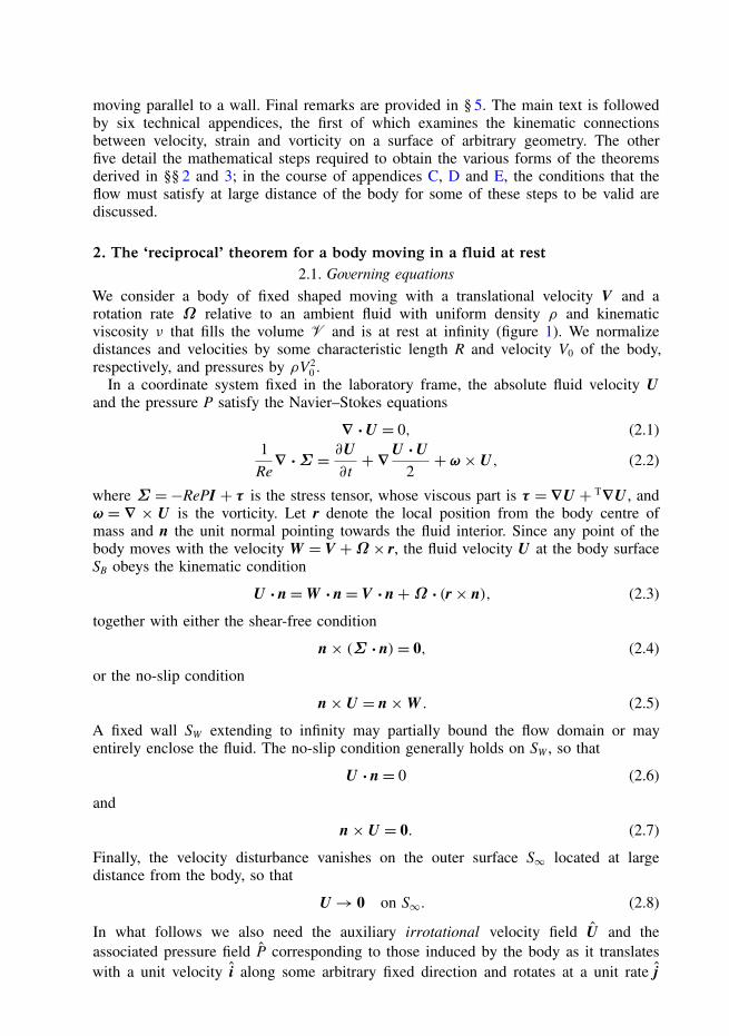
We consider a body of fixed shaped moving with a translational velocity V and arotation rate Ω relative to an ambient fluid with uniform density ρ and kinematicviscosity ν that fills the volume V and is at rest at infinity (figure 1). We normalizedistances and velocities by some characteristic length R and velocity V0 of the body,respectively, and pressures by ρV2

0 .In a coordinate system fixed in the laboratory frame, the absolute fluid velocity U

and the pressure P satisfy the Navier–Stokes equations

∇ ·U = 0, (2.1)1Re∇ ·Σ = ∂U

∂t+∇U ·U

2+ ω × U, (2.2)

where Σ =−RePI + τ is the stress tensor, whose viscous part is τ =∇U + T∇U , andω = ∇ × U is the vorticity. Let r denote the local position from the body centre ofmass and n the unit normal pointing towards the fluid interior. Since any point of thebody moves with the velocity W = V +Ω × r, the fluid velocity U at the body surfaceSB obeys the kinematic condition

U ·n=W ·n= V ·n+Ω · (r× n), (2.3)

together with either the shear-free condition

n× (Σ ·n)= 0, (2.4)

or the no-slip condition

n× U = n×W . (2.5)

A fixed wall SW extending to infinity may partially bound the flow domain or mayentirely enclose the fluid. The no-slip condition generally holds on SW , so that

U ·n= 0 (2.6)

and

n× U = 0. (2.7)

Finally, the velocity disturbance vanishes on the outer surface S∞ located at largedistance from the body, so that

U→ 0 on S∞. (2.8)

In what follows we also need the auxiliary irrotational velocity field U and theassociated pressure field P corresponding to those induced by the body as it translateswith a unit velocity i along some arbitrary fixed direction and rotates at a unit rate j

UU(x,t)

V(t)

O

r0

n

SB

SW

S

i

j

FIGURE 1. Sketch of the general flow configuration. The undisturbed velocity field UU(x, t)is non-zero only in § 3. In the auxiliary problem, the body translates with a unit velocity alongthe i direction and rotates with a unit rotation rate about the j axis, the fluid being at rest atinfinity.

about an arbitrary fixed axis passing through the origin O of the coordinate system.This auxiliary velocity field is governed by

∇ · U = 0, (2.9)

1Re∇ · Σ = ∂U

∂t+∇ U · U

2, (2.10)

where Σ = −RePI + τ , with τ = ∇U + T∇U . We may then introduce the velocitypotential φ such that U = ∇φ. In cases in which the flow domain is not simplyconnected, φ is made unique by requiring that there is no circulation around the body.The momentum balance for this viscous potential flow yields two separate conditionsvalid throughout the flow domain V , namely

∇ · τ =−∇ × (∇ × U)= 0, (2.11)

and the Bernoulli integral

∂φ

∂t+ U · U

2+ P= C(t), (2.12)

where C is a constant. As will be seen later, the condition (2.11), which expresses theproperty of zero flux of viscous stresses in an irrotational incompressible flow, plays akey role in the derivation of the theorem.

Owing to the irrotationality constraint, U only satisfies the kinematic condition atthe body surface SB and on the wall SW . Hence denoting with r0(t) the position of thebody centre of mass with respect to the origin of the coordinate system and definingW = i+ j × (r+ r0)= I + j × r with I = i+ j × r0, one has

U ·n= ∂φ∂n= W ·n on SB, (2.13)

U ·n= 0 on SW, (2.14)

while at large distances one has

U→ 0 on S∞. (2.15)

2.2. Derivation of the theoremDuplicating the classical procedure employed to establish reciprocal theorems, we startby forming the difference between the dot product of (2.2) and U and that of (2.11)and U , so as to eliminate the pseudo-dissipation rate 2Re−1τ : τ . Then, integrating overV , making use of the divergence theorem and of the divergence-free condition yields∫

SB∪SW

U ·[

1Re

Σ ·n− 12(U ·U)n

]dS

= 1Re

∫SB

U · (τ ·n) dS−∫

V

[∂U∂t+ ω × U

]· U dV, (2.16)

where the no-slip condition (2.7) has been assumed to hold on SW . Contributions fromS∞ vanish as r = ‖r‖ → ∞, thanks to the r−3 decay of U . Similarly, the volumeintegral on the right-hand side of (2.16) is convergent, provided U decays as r−n withn> 0 (and hence ω decays as r−n−1) in the wake of the body.

Conditions (2.13) and (2.14) allow the left-hand side of (2.16) to be transformedinto ∫

SB∪SW

U ·

1Re

Σ ·n− 12(U ·U)n

dS

= I ·F+ j ·Γ −∫

SB

12(U ·U)W ·n dS

+ 1Re

∫SW

US · (τ ·n)S dS+ 1Re

∫SB

(U − W )S ·(τ ·n)S dS, (2.17)

where F= Re−1∫

SBΣ ·n dS and Γ = Re−1

∫SBr×(Σ ·n) dS are the hydrodynamic force

and torque experienced by the body, respectively, and the subscript index S denotes thetangential component of the corresponding vector (for instance, US = n× (U×n)). Thelast term in (2.17) vanishes for a bubble submitted to the shear-free condition (2.4).

A series of manipulations based on the kinematic results established in appendix Aand on the Stokes theorem are then required to make vorticity apparent in theviscous contributions on SB in (2.16) and (2.17), irrespective of the dynamic boundarycondition that holds at the body surface. Similarly, the volume contribution involvingthe acceleration ∂U/∂t in (2.16) may be transformed to make added-mass effectsapparent by employing Leibnitz’s rule and the divergence theorem. The details of thesetransformations are given in appendix B. Making use of (B 1) and (B 7), (2.16) finallyyields the desired ‘reciprocal’ theorem in the form

I ·F+ j ·Γ = dW

dt

∫SB

φW ·n dS+∫

SB

(12U ·U

)W − Dφ

DtW

·n dS

− 1Re

∫SB

(U − W )× (ω − 2Ω)

·n dS− 2

Rej ·∫

SB

n× (U −W ) dS

−∫

V

(ω × U) · U dV − 1Re

∫SW

(U × ω) ·n dS, (2.18)

where dW/dt is the time derivative following the motion of the body centre of mass,D/Dt = ∂/∂t+U ·∇ is the material derivative, and (A 6) has been employed to expressthe contribution of the shear stress (τ ·n)S on SW in terms of vorticity. All the termsin (2.18) have a straightforward physical interpretation, except for the second term onthe right-hand side. However, another series of transformations detailed in appendix Cand involving Green’s second identity and repeated use of the divergence theoremmay be applied to that term. In the course of these transformations, it is natural tointroduce the bound vorticity ωB = n × (U − ∇Φ)δB, δB being the Dirac function,which is zero everywhere except on SB. This bound vorticity is due to the differenceat the body surface between the tangential component of the actual velocity field Uand that of the virtual irrotational velocity field ∇Φ that satisfies the same kinematicboundary conditions (2.3) and (2.6) on SB and SW . Then, provided the decay of theflow disturbance in the far field is fast enough (see below), use can be made of (C 9)so as to write (2.18) in the physically clearer form

I ·F+ j ·Γ = dW

dt

∫SB

φW ·n dS+∫

V

(ω + ωB)× U · (W − U) dV

− 1Re

∫SB

[(U − W )× (ω − 2Ω)] ·n+ 2j · [n× (U −W )] dS

−∫

SW

12(U ·U)W ·n+ 1

Re(U × ω) ·n

dS. (2.19)

A final step may be carried out to recast the first integral on the right-hand side of(2.19) in terms of elementary classical added-mass contributions. Thanks to the lineardependence of φ with respect to I and j emphasized by (2.13), one may set

φ =ΨT · I +ΨR · j, (2.20)

where the two vectors ΨT and ΨR are harmonic functions that, according to (2.13) and(2.14), satisfy

∂ΨT

∂n= n and

∂ΨR

∂n= r× n on SB, (2.21)

∂ΨT

∂n= 0 and

∂ΨR

∂n= 0 on SW . (2.22)

Introducing the usual second-order added-mass tensors A, B, C and D such that

A= TA=−∫

SB

ΨT∂ΨT

∂ndS, B = TC =−

∫SB

ΨT∂ΨR

∂ndS, (2.23)

C = TB =−∫

SB

ΨR∂ΨT

∂ndS, D = TD =−

∫SB

ΨR∂ΨR

∂ndS, (2.24)

one has

−∫

SB

φW ·n dS= I · (A ·V + B ·Ω)+ j · (C ·V + D ·Ω). (2.25)

Keeping in mind that I = i+ j×r0, noting that dWr0/dt = V and that the time derivativeof any time-dependent vector Q in the laboratory frame and that in the reference framerotating with the body, say dΩ/dt, are related by dΩQ/dt = dWQ/dt − Ω × Q, one

obtains in the most general case

−dW

dt

∫SB

φW ·n dS = I ·

dΩ(A ·V)dt

+ dΩ(B ·Ω)dt

+Ω × (A ·V + B ·Ω)

+ j ·

V × (A ·V + B ·Ω)+ dΩ(C ·V)

dt+ dΩ(D ·Ω)

dt

+Ω × (C ·V + D ·Ω)

, (2.26)

where the derivatives dΩA/dt = V ·∇A etc. are non-zero only if the body moves in thepresence of a wall and its velocity V has a non-zero component perpendicular to thatwall.

2.3. The various contributions to the force and torqueIn the specific case of a rigid body subject to a no-slip condition and moving in anunbounded fluid, (2.19) is equivalent to the separate expressions (2.24) for the forceand (3.7) for the torque obtained by Howe (1995). When the body moves in a boundedfluid, the expression for the force in (2.18) is also equivalent to equation (6) of GrottaRagazzo & Tabak (2007).

The interpretation of all the contributions on the right-hand side of (2.19) is clear.The first term, which is entirely determined by the auxiliary potential φ and thekinematic boundary condition at the body surface, represents the so-called added-massloads. This contribution is independent of any effects of both vorticity and viscosity(Mougin & Magnaudet 2002). Consequently, it is not influenced by any possibleseparation of the flow past the body, although this is sometimes erroneously thought tobe the case. Note that this is the only contribution to the force and torque involvingthe current fluid acceleration. The second term represents the contribution resultingfrom the presence of vorticity in the body of the fluid (the so-called free vorticity),supplemented by that of the bound vorticity on SB. Note that, on SB, W − U is tangentto the body surface owing to the kinematic condition (2.3). Therefore, in the vicinityof the body, the leading contribution to this volume integral comes from fluid elementsfor which the cross product between ω and U has a non-zero component tangent to SB.This remark helps one to appreciate correctly the role of boundary layers in the totalforce. The third term is due to the dynamic boundary condition at the body surface.Hence it represents the viscous loads produced by the surface vorticity (often referredto as skin friction when the no-slip condition applies). If the body is submitted to ashear-free condition, the slip between the body and the fluid results in an additionalviscous contribution to the torque that was not present in Howe’s equation (3.7), nor inequation (17) of Grotta Ragazzo & Tabak (2007), since both groups only consideredthe torque balance on a body obeying a no-slip condition. The fourth term results fromthe presence of the wall and generally comprises an inertial and a viscous contribution.The former, which is non-zero only if the fluid is able to slip along the wall (e.g.when SW is a symmetry plane), does not contribute to the force in the directionparallel to the wall, since W · n = I · n = 0 in that case. In contrast, whatever thedirection of the body motion, this term results in an additional non-zero force normalto the wall and in a torque. When the no-slip condition holds on SW , this inertialcontribution is still physically present but takes a different form in (2.19); indeedit may then be shown that it results from the near-wall contribution to the volumeintegral

∫V(ω × U) · (W − U) dV (this may be established by splitting U into an outer

and an inner contribution, the latter being due to the no-slip condition on SW , andusing arguments similar to those employed later at the end of § 4.1).

The viscous contribution on SW vanishes if the wall reduces to a symmetry planesince the vorticity may only have a normal component on such a surface. In thatcase there is also an extra viscous term Re−1

∫SW

US · (τ ·n)S dS in (2.16), but thiscontribution also vanishes since the tangential stress (τ ·n)S is zero by virtue of (A 9).From the above remarks it can be concluded in particular that a symmetry plane doesnot provide any contribution to the drag force, be it viscous or inertial, when thebody translates parallel to it. Thus D’Alembert’s paradox still holds for such a body insteady motion in a viscous potential flow.

2.4. Influence of the flow behaviour at large distance from the body

Some comments about the conditions that the flow disturbance must fulfil on S∞for the transformation from (2.18) into (2.19) to be valid seem in order. From atheoretical point of view, the compactness of the vorticity distribution, i.e. the fact thatω is vanishingly small outside a finite region of the control volume V over whichintegration is carried out, suffices to guarantee that all integrals on S∞ vanish whenthe surface recedes to infinity. In cases in which ω is not naturally compact withinV , the difficulty is classically by-passed by defining an extended vorticity distributionwithin the body volume VB of surface SB and beyond the outer surface S∞ of Vso as to reconnect properly the vortex tubes that cross SB and S∞. Integration maythen be performed within the extended control volume V+ of outer surface S+ inwhich all vortex tubes are closed and vorticity is vanishingly small outside some finitesubvolume Vω (Batchelor 1967; Saffman 1992). Then the velocity field is irrotationalwithin V+ − Vω and the Biot–Savart law implies that it decays like r−3 with thedistance r to the body at large distances from Vω, which guarantees the convergenceof the various integrals on V+ and S+. Therefore (2.19) is always a valid theoreticalresult.

The situation may be different if one is to use the present results to evaluatethe various contributions to the force or torque by post-processing direct numericalsimulation (DNS) data, as has been done in several studies (Chang & Chern 1991;Protas et al. 2000; Pan & Chew 2002; Chang et al. 2008). In DNS it is generallynot possible to use a control volume satisfying the above properties. Althoughthe computational domain VC extends far downstream from the body, vortices aregenerally shed across part of the surface SD that bounds it externally. Hence, withinsome parts of VC, velocities decay much more slowly than r−3 and may remainsignificant on parts of SD. For instance, if an axisymmetric (Oseen) wake crosses SD

normally, the normal velocity on this downstream surface is of O(r−1) within the wakeand of O(r−2) outside it (Batchelor 1967). Under such conditions, several technicalsteps used in the transformation from (2.18) to (2.19) may no longer be legitimate, asthey may result in finite or even diverging contributions on SD and diverging volumeintegrals over VC (see the discussion in appendix C after (C 7)). This is why it is thennecessary to examine carefully how the actual velocity field decays at large r beforetrying to compare computational results with (2.19). In summary, the main messageto be kept in mind is that the form (2.19) of the ‘reciprocal’ theorem is certainly notalways appropriate to compare DNS results with theoretical predictions, whereas theform (2.18) remains valid whatever the decay rate of the velocity disturbance in the farfield.

3. A body moving in a non-uniform flow3.1. The generalized form of the theorem

It is obviously of great interest to examine how the above theorem may be extended tothe general case of a body moving in an ambient non-uniform flow. The determinationof forces and torques acting on bodies immersed in such flows has been a subjectof active research since the pioneering works of Taylor (1928) and Tollmien (1938),who performed experiments on bodies of various shapes held fixed in converging,diverging or curved channels. Using an energy method, they also derived approximateexpressions for the inviscid force and torque acting on non-rotating bodies placedin an irrotational weakly non-uniform stream. Since then, the problem has beenreconsidered in greater generality by Galper & Miloh (1994, 1995) in the caseof rotating bodies of arbitrary shape moving in an irrotational linear flow field.Obviously, the case of ambient non-uniform flows with non-zero vorticity posesmuch greater difficulties. Combining a direct evaluation of the force in the case ofa two-dimensional circular cylinder with an asymptotic estimate of leading-order forcecontributions in the case of a sphere (which in particular makes use of the predictionfor the stationary inviscid shear-induced lift force obtained by Auton (1987)), Auton,Hunt & Prud’homme (1988) derived an expression for the inviscid hydrodynamic forceacting on point-symmetric bodies moving in a weakly unsteady, slowly varying, linearflow. The problem was revisited by Miloh (2003), who obtained expressions for theinviscid force and torque acting on rotating and translating bodies of arbitrary shapemoving in a general linear flow field, with no restriction on the relative magnitudeof the inhomogeneity, nor on that of unsteady effects. However Miloh’s results wereobtained under the highly restrictive assumption that the vorticity disturbance due tothe distortion of the ambient vorticity by the body remains negligibly small, whichprevents his results from being applicable to three-dimensional bodies, except at veryshort time after they have been introduced into the flow. The purpose of the presentsection is to extend the ‘reciprocal’ theorem derived in the previous section to suchnon-uniform situations so as to remove the limitations of the previous studies. Theresults available in the aforementioned literature should then be recovered as particularcases corresponding to the inviscid limit and to an unbounded flow domain.

To this end, let us consider the undisturbed incompressible flow whose velocity andpressure fields are UU(r + r0, t) and PU(r + r0, t), respectively. If the flow domain ispartially bounded by a wall, UU satisfies the corresponding boundary conditions on SW .In particular, one always has UU ·n= 0 on SW . It is then suitable to work with the flowdisturbance U = U − UU, which obeys

∇ · U = 0, (3.1)1Re∇ · Σ =

∂

∂t+ UU ·∇

U + ω × U + 1

2∇(U · U)+ U ·∇UU, (3.2)

U ·n= 0 and U × n= 0 on SW, (3.3)

U→ 0 on S∞, (3.4)

where Σ =Σ −ΣU and ω = ω − ωU, with ΣU and ωU denoting the stress tensor andthe vorticity associated with the undisturbed flow, respectively. Except for the last termon the right-hand side, which is intrinsically new, (3.2) is formally identical to (2.2)provided the time derivative ∂/∂t is replaced by the Lagrangian derivative followingthe undisturbed flow DU/Dt = ∂/∂t + UU · ∇. Similarly, provided W is changed intoW =W −UU = V −UU+Ω × r, the kinematic boundary condition (2.3) still holds for

the disturbance velocity U . It is then straightforward to obtain the counterpart of (2.18)in the presence of a non-uniform underlying flow except for two points. First oneneeds to establish how terms involving DUU/Dt transform. Then one has to considerthe contributions on S∞ encountered during the derivation and establish the conditionsunder which they are vanishingly small. Both points are addressed in appendix D.Combining the results of this appendix, especially (D 2), with the above remarks allowmost other steps leading to (2.18) to be readily repeated so as to obtain

I ·F+ j ·Γ = I ·FU + j ·ΓU + dW

dt

∫SB

φW ·n dS−∫

SB

DφDt

W ·n dS

+ 12

∫SB

(U · U)W ·n dS−∫

V

(ω × U) · U dV − 2∫

V

(U ·∇UU) · U dV

− 1Re

∫SB

(U − W )× (ω − 2Ω) ·n dS− 2Re

j ·∫

SB

n× (U − W ) dS

+ 1Re

∫SB

(U − W )(τU ·n)− UU · (τ ·n) dS

− 1Re

∫SW

(U × ω) ·n dS, (3.5)

where FU = Re−1∫

SBΣU ·n dS and ΓU = Re−1

∫SBr× (ΣU ·n) dS are the hydrodynamic

force and torque exerted by the undisturbed flow on the volume of fluid VB enclosedby SB, and τU = Re−1(∇UU + T∇UU).

Again, it is desirable to transform to fourth and fifth terms on the right-hand sideof (3.5) to allow for a clearer physical interpretation of the result. The correspondingtransformations are detailed in appendix E. Provided the required conditions hold forsome of these transformations to be valid (see again the discussion in § 2.4), (E 8)allows (3.5) to be finally recast in the form

I ·F+ j ·Γ = I ·FU + j ·ΓU + dW

dt

∫SB

φW ·n dS−∫

SB

Φ(j × UU) ·n dS

+∫

SB

ΦW ·∇UU ·n dS−∫

V

(ωU × U) · U dV

+∫

V

[(ω + ωB)× U] · (W − U) dV

− 1Re

∫SB

(U − W )× (ω − 2Ω) ·n dS− 2Re

j ·∫

SB

n× (U − W ) dS

+ 1Re

∫SB

(U − W )(τU ·n)− UU · (τ ·n) dS

−∫

SW

12(U · U)W + 1

ReU × ω

·n dS, (3.6)

where the velocity potential Φ satisfies n · ∇Φ = W · n on SB and n · ∇Φ = 0 onSW and the bound vorticity is now defined as ωB = n × (U − ∇Φ)δB. The first twoterms on the right-hand side of (3.6) represent the body force and torque resultingfrom the possible acceleration of the undisturbed flow, while the sum of the next twoterms is the added-mass contribution. Three extra terms result from the non-uniformity

of the undisturbed flow. Two of them involving either ∇UU or τU appear in theform of surface integrals on SB and generally provide non-zero contributions evenwhen the undisturbed flow is irrotational. There is also a third, contribution throughoutV involving the possible non-zero vorticity ωU of the undisturbed flow. Since thecorresponding term takes the form of the cross product of ωU by the relative velocityU , it clearly provides a lift component to the force experienced by the body.

The form (3.6) of the ‘reciprocal’ theorem is the most general result derived inthis paper, since it is valid for any undisturbed flow provided the conditions for thevanishing of contributions on S∞ established in appendix D are satisfied. Note that,if UU is uniform, it may readily be proved that (3.6) satisfies Galilean invariance, asit should. This may be seen by noting that (B 3) implies that

∫SBUU · (τ · n) dS = 0

when UU is uniform and by using (2.25) and (2.26), which show that the added-masscontribution keeps the same form as in the case of a fluid at rest, except for the factthat V has to be replaced by V = V − UU everywhere in (2.26).

3.2. A body in a general linear flow

To reveal the various effects of the undisturbed velocity gradients, we now specialize(3.6) to the widely encountered situation where the carrying flow can be consideredlinear, in which case

UU(r0, r, t)= U0(r0, t)+ r ·∇U0(t)= U0(r0, t)+ r ·S0(t)+ 12ω0(t)× r, (3.7)

where r0 still denotes the instantaneous position of the body centre of mass, andS0 and ω0 are the constant-strain-rate tensor and vorticity of the undisturbed flow,respectively. Note that the presence of a wall imposes severe restrictions on the formof the linear flow that may exist in V , owing to the kinematic boundary conditionUU · n = 0 on SW . For instance, if ω0 = 0 and the undisturbed flow is a planarextensional flow, SW may be one of the two symmetry planes of that flow. Similarly,if S0 = 0 and the flow configuration corresponds to a solid-body rotation in a circularcylinder, SW may be the lateral wall of the cylinder.

The kinematic boundary condition at the body surface now reads

W ·n= V ·n+ Ω · (r× n)− 12 S0 : (rn+ nr), (3.8)

where V(r0, t) = V − U0 and Ω(t) =Ω − ω0/2. Hence the velocity potential Φ takesthe form

Φ =ΨT · V +ΨR · Ω −ΨS : S0, (3.9)

where ΨT and ΨR have been defined in § 2.2 and ΨS is a symmetric second-ordertensor satisfying

∇2ΨS = 0 in V,∂ΨS

∂n= 1

2(rn+ nr) on SB,

∂ΨS

∂n= 0 on SW . (3.10)

From (3.8) we deduce that the integral∫

SBφW ·n dS may be expressed in the form

−∫

SB

φW ·n dS = I · (A · V + B · Ω − ET : S0)

+ j · (C · V + D · Ω − ER : S0), (3.11)

where ET and ER are two third-order tensors, respectively defined by

ET =∫

SB

ΨT∂ΨS

∂ndS=

∫SB

∂ΨT

∂nΨS dS,

ER =∫

SB

ΨR∂ΨS

∂ndS=

∫SB

∂ΨR

∂nΨS dS.

(3.12)

The form (3.9) of the velocity potential makes it clear that quadratic contributions withrespect to ω0 and S0 are present in every inertial term of (3.6). However, to avoid toocumbersome formulae while capturing the leading effects of the inhomogeneity, weshall neglect these terms and consider only linear contributions. This simplification isbased on the assumption that, in many situations of practical interest, ‖r ·S0‖/‖V‖ 1and ‖r×ω0‖/‖V‖ 1 for ‖r‖ = O(1), i.e. the typical length scale of the body is smallcompared to the characteristic length scale of the inhomogeneity. Quadratic terms havebeen considered in the inviscid approximation, either in the irrotational case by Galper& Miloh (1995) or in the short-time limit in rotational flows by Miloh (2003). Aconsequence of the above assumption is that ω0 must be considered independent oftime from now on, since in a linear flow the evolution of the vorticity is governed bythe Helmholtz equation dω0/dt = ω0 ·S0.

With a linear undisturbed flow, the viscous contribution at the body surface in(3.6) may be simplified by recognizing that ∇ · τU = 0, a property implying that∫

SBW · (τU ·n) dS= 0. Since τ is also divergence-free, Green’s second identity implies

that∫

SB∪SWU · (τU · n) − UU · (τ · n) dS = 0, which allows the contribution of the

undisturbed flow on SB to be transformed into a contribution on SW . Applying the‘weak inhomogeneity’ approximation defined above, (3.6) then becomes

I ·F+ j ·Γ = I ·F0 + j ·Γ0 + dW

dt

∫SB

φW ·n dS− (j × U0) ·

∫SB

Φn dS

+∫

SB

Φ0W ·∇U0 − j × (r ·∇U0) ·n dS

+∫

V

[(ω + ωB)× U]0 ·(W − U) dV −∫

V

(ω0 × U0) · U dV

− 1Re

∫SB

(U − W )× (ω − 2Ω) ·n dS

− 2Re

j ·∫

SB

n× (U − W ) dS

−∫

SW

12(U · U)0 W +

1Re

U × ω·n dS, (3.13)

where Φ0 =ΨT · V + ΨR ·Ω and U0 = U − U0, and [(ω + ωB)× U]0 (respectively,(U · U)0) denotes the corresponding cross product (respectively, dot product) linearizedin the sense defined above. In (3.13), F0 = (D0U0/Dt)VB = ∂U0/∂t + U0 · ∇U0VB isthe linearized body force acting on the volume VB and Γ0 =

∫VB

r × (r · dS0/dt) dVis the associated body torque, which is non-zero only if the undisturbed velocitygradients are time-dependent (the contribution

∫SBr × (D0U0/Dt) dS to the torque is

zero since r = 0 corresponds to the body centre of mass). Note that the vortical part

of the viscous contributions on both SB and SW involves the total vorticity ω, not thevorticity disturbance ω.

To obtain a detailed view of the effects produced by the base flow, two moresteps are necessary. First, all inertial contributions over the body surface (first threeintegrals on the right-hand side of (3.13)) must be expanded with respect to S0, ω0

and D0U0/Dt. The result of this expansion is provided by (F 1)–(F 4) in appendix F.Then the volume integral involving ω0 must be transformed so as to disentanglecontributions provided by the potential and vortical parts of the velocity disturbanceU0. This transformation yields (F 6), which reveals the existence of the surfacecontribution ω0 ·

∫SBφ(n × ∇Φ0) dS, which only depends on the irrotational velocity

field ∇Φ0 and hence may, under certain conditions, be connected to the added-masstensor.

Results (F 1)–(F 6) may finally be injected into (3.13) to obtain the final form of the‘reciprocal’ theorem in a linear flow without any restriction on the body shape (but stillin the weakly inhomogeneous approximation). As (F 2)–(F 4) make clear, numerouscouplings between the body rotation Ω and the strain rate S0 or the ambient vorticityω0 contribute to the force and torque balances in the case of a general body shape.Those that subsist when the carrying flow is irrotational have been examined by Galper& Miloh (1994, 1995) and the discussion will not be repeated here.

Fortunately, applications frequently involve bodies exhibiting geometricalsymmetries that suppress most of these couplings and clarify the interpretation of themost important physical effects. Here we focus on the class of bodies exhibiting threeorthogonal symmetry planes, which in particular encompasses axisymmetric bodieswith fore–aft symmetry, among which are ellipsoids. However, even for such simplebody geometries, the presence of a wall still maintains couplings between translationaland rotational motions. Therefore, only two physical situations lead to significantsimplifications. The first of these corresponds to the case of an unbounded flowdomain or equivalently to a situation where the body moves at large distance fromthe wall so that wall effects can be ignored. The second corresponds to the situationwhere the body moves close to a plane wall without rotating, one of its symmetryplanes being parallel to that wall. For such body shapes and flow conditions, theirrotational disturbance induced by the translational motion becomes uncoupled withthose resulting from rotation (if any) and deformation. Hence ET = 0 and the onlytwo added-mass tensors that subsist are A and D. Moreover, as shown by (F 7) and(F 8), all contributions to the torque involving the combined effect of the possiblebody rotation Ω and of the background vorticity ω0 are expressible via the third-ordertensor K defined through the relation D = 2(K · J) : ε, where J = ∫

VB(r · r)I − rr dV

is the inertia tensor and ε denotes the usual third-order alternating tensor.Thus, making use of the various results established in appendix F, the form of

(3.13) suitable for bodies exhibiting the symmetries defined above and moving in anunbounded flow domain is finally found to be

I ·F+ j ·Γ

= I ·

D0U0

DtVB − A ·

(dVdt− D0U0

Dt−Ω × V

)−Ω × (A · V)

+ [A ·S0 − S0 ·A] · V +(I2+ A

VB

)· [ω0 × (A · V)] − 1

2A · (V × ω0)

− j ·V × (A · V)+ D ·

(dΩdt+ 1

2Ω × ω0

)+Ω ×

(D ·

(Ω − 1

2ω0

))+ER :

dS0

dt− 2ε : (Ω ·ER ·S0)+ 2(ER ·S0) : (Ω · ε)+Ω × (ER : S0)

− 4(K · J) · (TK ·Ω) : (ε ·ω0)− (Ω ·K ) · (J ·ω0)+ J · (ω0 ·TK ·Ω)

+∫

V

[(ω + ωB)× U]0 ·(W − U) dV −∫

V

φω0 · (ω + ωB)0 dV

− 1Re

∫SB

(U − W )× (ω − 2Ω) ·n dS

− 2Re

j ·∫

SB

n× (U − W ) dS, (3.14)

where the time derivatives are expressed in non-rotating axes and the integrand in thelast volume integral has been linearized in the sense defined above, so that (ω0 + ωB)0does not depend on S0 and ω0. Now the interaction of S0 with the body rotation Ωonly contributes to the torque. Moreover, most contributions to the torque related tothe ambient strain rate and vorticity in (3.14) vanish when the body does not rotate.More precisely, the only term due to the inhomogeneity of the undisturbed flow thatstill influences the torque when Ω = 0 is that associated with the possible unsteadinessof S0.

In (3.14) the ambient strain rate and vorticity contribute to the Lagrangianacceleration D0U0/Dt, whose direction is generally not aligned with that of thebody’s relative velocity V . In addition, the ambient strain rate still influences thehydrodynamic force through the term [A · S0 − S0 · A] · V , which is non-zero onlywhen the principal axes of S0 are not aligned with those of the body. In this case,this term is orthogonal to V and hence contributes to the lift force. The pair of terms12ω0× (A ·V)− 1

2 A ·(V ×ω0) also contributes to that component of the force. Moreover,these two contributions are supplemented by the term A · [ω0 × (A · V)]/VB resultingfrom (F 7), which is quadratic with respect to the translational added-mass tensor.For a point-symmetric body such as an infinitely long circular cylinder or a sphere,D = ER = K = 0 and A = A I , where A /VB is the usual added-mass coefficient.Hence the closed-form contributions to the torque vanish identically, whereas those tothe force reduce to (VB +A )D0U0/Dt −A dV/dt +A (1+A /VB)ω0 × V .

On the right-hand side of (3.14), all terms resulting from the inhomogeneity of theambient flow are similar to those obtained by Miloh (2003), although contributionsto the torque involving S0 and ω0 are expressed in a different way. However, thefundamental difference between the two sets of results is that Miloh’s derivationassumes an inviscid flow with a negligible vorticity disturbance throughout thefluid, so that all four volume and surface integrals in (3.14) do not appear. Whatthe present result shows is that the inviscid contributions predicted in Miloh’sapproach survive in the presence of viscous effects and of a non-zero vorticitydisturbance throughout the flow, and that a clear splitting between these variouseffects is naturally achieved by the extended form of the ‘reciprocal’ theoremderived in this section. The result (3.14) may also be seen as the generalizationto anisotropic bodies and to finite-Reynolds-number conditions of the well-knownexpression F = (VB + A )D0U0/Dt − A dV/dt + CLVBω0 × V derived in the inviscid

limit by Auton et al. (1988) in the particular case of a two-dimensional circularcylinder and a sphere moving in a weakly unsteady shear flow, respectively.

As pointed out above, the group of terms 12 ω0 × (A · V) + A · (ω0 × V) + A ·

[ω0 × (A · V)]/VB in (3.14) contributes to the lift force. Nevertheless, owing to theHelmholtz equation, the vorticity disturbance ω is generally non-zero in the presenceof an ambient vorticity ω0, even though the flow is considered inviscid, and thearrangement of ω and ωB around the body results in a non-zero value of the remainingvolume integrals that make additional contributions to this force. Therefore, evaluatingthe net lift force generally requires the vorticity disturbance (and velocity) to be knownthroughout the flow field, as exemplified by Auton’s calculation for the steady liftforce on a sphere in a weak shear flow (Auton 1987). It is only in particular situationsthat the inertial closed-form terms in (3.14) represent the entire lift force. Inviscidtwo-dimensional flows provide such a situation, since ω and ωB are both zero in thatcase, making both volume integrals in (3.14) vanish. For a two-dimensional circularcylinder, A /VB = 1, so that, when the cylinder moves in an inviscid shear flow withω0 parallel to its axis, the lift force is found to be 2VB ω0 × V , in agreement witha classical result (Batchelor 1967). In three-dimensional flows, although ω is zeroright at the time the body is introduced into the flow, the volume integrals in (3.14)become non-zero as the flow disturbance sets in, owing to the stretching/tilting termω0 · ∇U . Therefore it is only in the short-time limit that the above closed-form termsprovide the entire lift force. Miloh (2003) considered this limit for a sphere (for whichA /VB = 1/2), in which case (3.14) predicts that the lift force is 3

4VB ω0 × V , inagreement with the asymptotic determination of Legendre & Magnaudet (1998). Incontrast, in the nearly steady approximation considered by Auton et al. (1988), thevorticity disturbance around the sphere is non-zero, yielding CL = 1/2 in the abovesimplified form of F.

Finally, if the flow domain is bounded by a plane wall, the form of the ‘reciprocal’theorem suitable for a non-rotating body having one of its three symmetry planesparallel to the wall is

I ·F+ j ·Γ = I ·

D0U0

DtVB − A ·

(dVdt− D0U0

Dt

)− (V ·∇A) · V

+ [A ·S0 − S0 ·A] · V +(I2+ A

VB

)×[ω0 × (A · V)] − 1

2A · (V × ω0)

− j ·

V × (A · V)+ ER :

dS0

dt− 1

2(V ·∇D) ·ω0 + (V ·∇ER) : S0

−∫

V

φω0 · (ω + ωB)0 dV +∫

V

[(ω + ωB)× U]0 ·(W − U) dV

− 1Re

∫SB

(U − W )× (ω − 2Ω) ·n dS− 2Re

j ·∫

SB

n× (U − W ) dS

−∫

SW

12(U · U)0 W + φU0 × ω0 + 1

ReU × ω

·n dS. (3.15)

Note that (3.15) is still valid for a rotating circular cylinder or a rotating spheresince rotation does not induce any inviscid effect for such point-symmetric bodies. In

addition, ER = D = 0 in that case, so that the last three terms in the expression forthe torque vanish. In contrast, A is generally not spherical even for point-symmetricbodies, since the added-mass coefficients corresponding to an acceleration parallel orperpendicular to the wall may differ from each other.

4. Some applications to high-Reynolds-number bubble dynamicsIn this section we consider three applications of the various forms of the theorem

derived in §§ 2 and 3 to the prediction of high-Reynolds-number bubble motion. Thefact that the surface vorticity generated by the shear-free boundary condition is ofO(1) (once normalized by the ratio of the slip velocity V0 over some characteristiclength scale R of the bubble) instead of being of O(Re1/2) when the no-slip conditionholds makes viscous corrections much weaker for bubbles than for solid bodies. Moreprecisely, the normalized tangential velocity changes by O(Re−1/2) within the boundarylayer surrounding a bubble, instead of changing by O(1) near a no-slip surface (Moore1963; Batchelor 1967). Therefore, in the limit of very large Reynolds number, thebound vorticity ωB in (2.19) (or ωB in (3.6)) is negligibly small and the effect ofthe shear-free condition can be considered as merely resulting in a vortex sheet rightat the bubble surface. This major difference with solid bodies makes it possibleto perform asymptotic calculations in the limit Re→∞ so as to obtain consistentforce and torque expressions including both inertial and leading-order viscous effects.Conversely, in situations where inviscid theory predicts a non-zero force or torque,viscous effects can only induce a small correction to that prediction, not a contributionof similar or even larger magnitude as may be the case with the no-slip condition.For these reasons it sounds interesting to examine how results derived in the previoussections may be applied to predict inertial and/or viscous loads on shear-free bubblesin some contrasting situations.

4.1. Two spherical bubbles rising side by side in a liquid at rest

To illustrate the ability of (2.19) to predict both drag and lift components of theforce, we first consider how it applies to the well-understood situation of twoidentical spherical bubbles rising steadily in such a way that their line of centresstays perpendicular to their rise velocity (Legendre, Magnaudet & Mougin 2003). Thedimensional distance between the two bubbles is 2L, so that it is convenient to definethe dimensionless quantity κ = R/L, which represents the inverse of the separationfrom one bubble to the symmetry plane of the system. Hence this symmetry plane nowstands at r · e⊥ = −1/κ , where e⊥ is the unit vector in the direction of the line ofcentres pointing away from the symmetry plane (figure 2a). We assume the separationL to be much larger than the bubble radius R, i.e. we consider the limit κ 1. In afirst step we assume that the Reynolds number is infinite but the fluid is still viscous,so that the velocity disturbance may be considered irrotational except right at thesurface of the bubbles. Corrections related to the finiteness of Re will be consideredlater. Consequently, at leading order in Re−1 and in κ (i.e. in the limit κ → 0), thevelocity disturbance about the bubble centred at r = 0 (say bubble A) is merely thedipole solution U0 = −V · ∇(r/2r3) (hence V is the rise velocity in the limit κ→ 0).To cancel the normal velocity created by this dipole on the symmetry plane, a dipoleof similar strength must be introduced at the image point r = −(2/κ)e⊥ (i.e. at thecentre of the second bubble, say B). The velocity field induced by this image dipole isof course U∗0 =−V ·∇(r∗/2r∗3), with r∗ = r+ 2κ−1e⊥ and r∗ = ‖r∗‖. Expanding U∗0 in

V V V

e

e e

e

SW

UU(r)

(a) (b)

FIGURE 2. Flow configurations considered in (a) § 4.1 and (b) § 4.3.

the vicinity of bubble A yields

U∗0 (κ‖r‖ 1)= U∞(r)=−κ3

16V + 3κ4

32((e⊥ · r)V + (V · r)e⊥)+ O(κ5). (4.1)

Hence bubble A experiences a ‘far-field’ velocity made up of a uniform velocity−(κ3/16)V and a straining field (3κ4/32)((e⊥ ·r)V+(V ·r)e⊥). To satisfy the kinematiccondition (2.3) at the bubble surface up to terms of O(κ4), one has to add a dipoleand a quadrupole with the proper strengths. The final velocity field near bubble A thenreads

UA(r)= U∞(r)− 12

(1+ κ

3

16

)V ·∇

( rr3

)− κ

4

48

e⊥V :∇∇

( rr3

)+ O(κ5). (4.2)

The auxiliary velocity field required to apply the ‘reciprocal’ theorem inthe V direction corresponds to the particular choice W = i = V/‖V‖, so thatU = UA/‖V‖. Since the flow is steady, the first contribution on the right-hand sideof (2.19) is zero. The vorticity is zero except right on the bubble surface, whichindicates that the second contribution is also zero, although we do not know yet howit goes to zero when Re→∞. Moreover V · n = i · n = 0 on SW since the motion isparallel to the symmetry plane, so that there is no contribution from SW . Hence onlythe third integral is non-zero. The corresponding contribution is more easily evaluatedusing the form (B 6), namely

V ·F=−2‖V‖Re

∫SB

(UAS − VS) ·∇Sn · (US − VS) dS. (4.3)

In a system of spherical coordinates (r, θ, φ) with the axis θ = 0 corresponding tothe direction of V , we have VS = −eθ sin θ and the curvature tensor can be written as∇Sn= eθeθ + eφeφ . Evaluating (4.3) then yields

V ·F=−12Reπ

(1+ κ

3

8

)V ·V + O(κ6). (4.4)

Hence, provided the volume integral on the right-hand side of (2.19) decays faster thanRe−1 when Re→∞ (which we shall show later to be the case), the leading-orderdrag is given by (4.4), so that the dimensional drag is F = −12πρνRV0(1 + κ3/8)V .

This prediction agrees with that derived by Kok (1992) at O(κ3) in the limitκ 1, Re→∞ using the ‘dissipation’ theorem. When κ → 0, the above resultobviously corresponds to Levich’s prediction for the drag of a single spherical bubblerising with an infinitely large Reynolds number in an unbounded liquid at rest atinfinity (Levich 1949, 1962; Batchelor 1967).

To make use now of (2.18) in the direction of the line of centres, we need theauxiliary velocity field corresponding to i = e⊥. By a similar method, we find that thevelocity field induced near bubble A by the corresponding image dipole is

U∞(r)= κ3

8e⊥ + 3κ4

32(r− 3(r · e⊥)e⊥)+ O(κ5). (4.5)

Hence, near bubble A, the required auxiliary velocity field correct up to terms of O(κ4)

is found to be

U(r)= U∞(r)− 12

(1− κ

3

8

)e⊥ ·∇

( rr3

)+ κ

4

32

e⊥e⊥ :∇∇

( rr3

)+ O(κ5). (4.6)

The force on the bubble can now be evaluated through (2.19) in which, still in thelimit of infinite Reynolds number, only the third integral and the first part of the fourthintegral can be non-zero. However, the integrand of the former is an even function ofthe angular position along the bubble surface and hence integrates to zero. To avoidthe determination of U on SW , the latter contribution may be evaluated using the form(2.18) together with (C 3), thanks to which one obtains

F · e⊥ =∫

SB

(12UA·UA

)e⊥ − (UA

· e⊥)V·n dS=− 3

16πκ4 + O(κ5). (4.7)

Therefore, at leading order, the dimensional transverse force is −(3/16)πκ4ρR2V20e⊥,

which is the classical result provided by irrotational flow theory (Milne-Thomson1968). However, what (4.7) additionally shows is that this prediction is notaltered by the non-zero vorticity present right at the bubble surface. We shallsee below how the contribution of the volume integral in (2.19), which dependson the vorticity distribution throughout the boundary layer, influences this forcecomponent.

To complete the determination of both components of F we need to evaluate theleading-order corrections induced by the finiteness of the Reynolds number. Thesecorrections are provided by the volume integral I = ∫

V(ω + ωB)× U · (W − U) dV

in (2.19). However, they can be more straightforwardly estimated by starting from theform (2.18) of the theorem. Then, splitting the complete velocity field about bubble Ainto the form U = UA + u, where u is the vortical correction that vanishes outside theboundary layer and wake, and making use of (C 4), we have

I +∫

SW

12(U ·U)W ·n dS =

∫SB

12(U ·U)W − Dφ

DtW

·n dS−

∫V

(ω × U) · U dV

=∫

SB

12(UA·UA)W − (UA

· W )W·n dS

+∫

SB

12(u ·u)W ·n dS

+∫

SB

(u ·UA)W − (u · U)W ·n dS

−∫

V

(ω × (UA + u)) · U dV. (4.8)

The first integral on the right-hand side is the irrotational contribution that leads to(4.7) when W = e⊥. The kinematic conditions (2.13) and (2.14) may be used totransform the second and third integrals on the right-hand side, the former becoming− 1

2

∫V∇(u · u) · U dV . The entire vortical contribution in (4.8) may then be written in

the form

I =∫

SB

u× (U × UA) ·n dS−∫

V

ω · (UA × U) dV −∫

V

(u ·∇u) · U dV. (4.9)

Selecting W = e‖ implies that UA = ‖V‖U , which shows that the first two integralson the right-hand side of (4.9) vanish. Up to terms of O(κ3), the boundary layerthat surrounds the bubble is axisymmetric and its characteristics are similar to thosedetermined by Moore (1963) for a single bubble moving at large Reynolds numberin a fluid at rest at infinity. Therefore the tangential (respectively, normal) componentof u is of O(Re−1/2) (respectively, O(Re−1)) within the O(Re−1/2)-thick boundarylayer. In the last integral of (4.9) the integrand is thus of O(Re−1), yielding anO(Re−3/2) contribution to the drag. Owing to the straining contribution in (4.1), thevortical velocity correction has an additional non-axisymmetric O(κ4) component. Inthe spherical coordinate system introduced above, this component, say uNA(r, θ, φ), isnecessarily a linear function of sinφ and cosφ, so that

∫ 2π0 uNA(r, θ, φ) dφ = 0. The

last integral in (4.9) involves contributions of the form∫

V(uA ·∇uNA+uNA ·∇uA) ·U dV

(uA denoting the axisymmetric part of u) but such terms are actually zero and thefirst correction to the drag provided by uNA is expected to be associated with the term∫

V(uNA ·∇uNA) ·U dV , which is of O(κ8). In other words, up to that order, the finite-Re

correction to (4.4) is merely that computed by Moore (1963), so that one has

V ·F=−12Reπ

(1+ κ

3

8

)(1− 1.56Re−1/2)V ·V + O(κ6), (4.10)

where it must be kept in mind that the present Reynolds number is based on thebubble radius, so that the factor 1.56 in (4.10) is equivalent to the more familiarfactor 2.21 in Moore’s original paper. The prediction (4.10) was already obtained byLegendre et al. (2003), who found that it agrees well with DNS results for Re > 20.Let us finally examine the contribution of I to the transverse force. Now UA and Uare no longer collinear, so that the first two integrals on the right-hand side of (4.9)are in principle non-zero and are dominated by contributions proportional to Re−1/2.However, within the boundary layer, the vorticity is dominated by the radial variationsof the tangential components of u, i.e. one has ω ≈ −(∂uφ/∂r)eθ + (∂uθ/∂r)eφ .Moreover, the relative variation of the irrotational fields UA and U across theboundary layer is only of O(Re−1/2), while that of uθ and uφ is of O(1) andboth vortical velocity components vanish at the outer edge of the boundary layer.Using these remarks and the kinematic conditions (2.13) and (2.14), the leading-order contribution to the first volume integral in (4.9) can be evaluated, yielding∫

Vω · (UA × U) dV ≈ ∫SB

(UAθ uθ + UA

φuφ)Wr − Wr(Uθuθ + Uφuφ) dS, which is justthe surface integral in (4.9); in other words, the leading contribution of ω to I

is balanced by that of the bound vorticity ωB. Hence, the first two integrals onthe right-hand side of (4.9) cancel at leading order and the first non-zero differencebetween them arises because of the O(Re−1/2) relative variations of UA and U acrossthe boundary layer and of the O(Re−1/2) secondary contributions to ω, yielding a netcontribution proportional to Re−1. Since the first non-axisymmetric component of ωarises at O(κ4), we conclude that the difference between the leading two integralsin (4.9) yields an O(κ4Re−1) contribution to the transverse force. Indeed, a viscouscorrection to that force component behaving as κ4Re−1 was detected numerically byLegendre et al. (2003), who observed it to be repulsive and found the correspondingprefactor to be approximately 7.5 with the present definitions.

From a theoretical point of view, evaluating this viscous contribution requiressolving the non-axisymmetric boundary layer problem at O(κ4). This is obviouslya significant effort that is beyond the scope of the present paper. Nevertheless,even at the present qualitative stage, the formulation (2.18)–(2.19) has the decisiveadvantage of providing a formal expression and an order-of-magnitude estimate ofthis contribution and of showing by which mechanisms it is generated. None ofthese conclusions could have been reached with the ‘dissipation’ theorem, since thisviscous transverse force does not produce any work. After the present investigationwas completed, it was realized that results (4.4) and (4.7) and several of the abovequalitative conclusions were already obtained using a formulation close to the presentone by Grotta Ragazzo & Tabak (2007).

4.2. Viscous force and torque on an oblate spheroidal bubble translating and rotating in aliquid at rest

Although the flow domain is unbounded and the fluid is at rest at infinity in thatcase, it is of interest to use (2.19) in order to evaluate all viscous contributionsthat can affect the motion of oblate spheroidal bubbles in the limit of very largeReynolds numbers, as this simplified geometry is known to provide a valid first-orderapproximation of the actual shape of millimetric bubbles moving in low-viscosityliquids (Magnaudet & Eames 2000). The corresponding inviscid contributions providedby the Kelvin–Kirchhoff equations or equivalently by the first integral on the right-hand side of (2.19) are well known and will not be discussed here (they correspond to(2.26) with B = C = 0 and dWA/dt = dWD/dt = 0).

Let us first introduce the classical oblate ellipsoidal coordinate system (ζ, µ, φ) suchthat (Lamb 1945)

x= kζµ, y= k (1+ ζ 2)1/2(1− µ2)

1/2cosφ,

z= k (1+ ζ 2)1/2(1− µ2)

1/2sinφ,

(4.11)

where k is a constant that determines the volume of the spheroid. For µ ∈ [−1, 1] andφ ∈ [0, 2π], the surface corresponding to ζ = ζ0 is that of an oblate ellipsoid of aspectratio χ = (1+ ζ 2

0 )1/2/ζ0 and volume V = 4πk3ζ0(1+ ζ 2

0 )/3. The corresponding metricfactors hµ, hζ and hφ are given by

hµ = k

(ζ 2 + µ2

1− µ2

)1/2

, hζ = k

(ζ 2 + µ2

1+ ζ 2

)1/2

,

hφ = k (1− µ2)1/2(1+ ζ 2)

1/2.

(4.12)

The surface curvature tensor ∇Sn may be written in the form ∇Sn = Hnµ(ζ0)eµeµ +

Hnφ(ζ0)eφeφ , where eµ and eφ are the unit vectors in the meridian and azimuthal

directions, respectively, and Hnµ and Hn

φ are the two radii of curvature, given by

Hnµ =

1hµhζ

∂hµ∂ζ= ζ (1+ ζ 2)

1/2

k (ζ 2 + µ2)3/2 ,

Hnφ =

1hφhζ

∂hφ∂ζ= ζ

k (1+ ζ 2)1/2(ζ 2 + µ2)

1/2 .

(4.13)

We assume that the minor axis of the bubble is aligned with the unit vector ex,whereas the equatorial plane is parallel to the (ey, ez) plane. According to Lamb(1945), the velocity potential corresponding to an incident velocity i and satisfying thekinematic condition (2.13) is φT =ΨT · i with

ΨT = kµ1− ζcot−1ζ

ζ0 (1+ ζ 20 )−1− cot−1ζ0

ex

+ k(1− µ2)

1/2[ζ/ (1+ ζ 2)1/2− (1+ ζ 2)

1/2 cot−1ζ ](2+ ζ 2

0 )ζ−10 (1+ ζ 2

0 )−1− cot−1ζ0

cosφey + sinφez. (4.14)

Similarly, the velocity potential corresponding to a rotation rate j is φR =ΨR · j with

ΨR = 13

k2µ (1− µ2)1/2 3ζ (1+ ζ 2)

1/2 cot−1ζ − (3ζ 2 + 2) (1+ ζ 2)−1/2

(1+ 2ζ 20 )cot−1ζ0 − 2ζ0 − ζ0/3 (1+ ζ 2

0 )−1

×sinφey − cosφez. (4.15)

Again, in the limit Re→∞, the velocity field U may be approximated by theirrotational form U = ΨT · V + ΨR ·Ω throughout the body of the flow. SelectingU = ∇ΨT · i and implementing the above expressions in the form (B 6) of the viscouscontribution to (2.19), the viscous force acting on the bubble is found to be

F=−4πkP‖exex + P⊥(eyey + ezez) ·V , (4.16)

with

P‖(ζ0)= (1− ζ 20 )ζ

−20 cot−1ζ0 + ζ−1

0

(1+ ζ 20 ) ζ0 (1+ ζ 2

0 )−1−cot−1ζ0

2 , (4.17)

P⊥(ζ0)= 2ζ0(1− ζ 2

0 )+ (1+ ζ 20 )

2 cot−1ζ0

(2+ ζ 20 )− ζ0(1+ ζ 2

0 )cot−1ζ02. (4.18)

The expression for the drag along the short axis agrees with that of Moore(1965), while that for the drag along any major axis agrees with the result derivedindependently by van Wijngaarden (2005) and by the present author (unpublished),all of them having made use of the ‘dissipation’ theorem in the limit Re→∞.The normalized drag coefficients 4kP‖ and 4kP⊥ are plotted as a function of theaspect ratio χ in figure 3. The above expressions indicate that the viscous force isgenerally not aligned with the upstream velocity since P‖ 6= P⊥. Actually P‖ is largerthan P⊥ and the difference increases as the bubble becomes more oblate, i.e. asζ0→∞. Hence the angle Ψ = sin−1(‖F − (F · ex)ex‖/‖F‖) is smaller than the driftangle Θ = sin−1(‖V − (V · ex)ex‖/‖V‖) and, the larger the oblateness, the larger thedifference Θ − Ψ . It is also worth noting that, given the geometrical symmetries of thesurface and the linearity of the viscous term in (2.19) with respect to the velocity, no

1 1.5 2 2.5

10

0

20N

orm

aliz

ed c

oeff

icie

nts

30

40

4kP⊥

4kP

4k3T

FIGURE 3. Evolution of the normalized drag and torque coefficients versus the bubble aspectratio χ = (1+ ζ 2

0 )1/2/ζ0 for 1 6 χ 6 2.5.

viscous contribution to the force can be induced by the rotation Ω . Hence there is noviscous Magnus-like force in the high-Re limit considered here.

As far as we are aware, no result is available in the literature for the viscous torqueacting on the bubble. Selecting U =∇ΨR ·j, long but straightforward calculations yield

Γ =−4πk3TΩ(eyey + ezez) ·Ω , (4.19)

with

TΩ(ζ0)= 118

Q2(ζ0)A(ζ0)− 13

Q(ζ0)B(ζ0)+ 12

C(ζ0), (4.20)

where

Q(ζ0)= 3(1+ ζ 20 )cot−1ζ0 − (3ζ 2

0 + 2)ζ−10

(1+ 2ζ 20 )(1+ ζ 2

0 )cot−1ζ0 − 2ζ0(1+ ζ 20 )− ζ0/3

, (4.21)

A(ζ0) = (1+ 2ζ 20 )(1− 6ζ 2

0 ) (1+ ζ 20 )

2cot−1ζ0

+ ζ0(1+ ζ 20 )(12ζ 4

0 + 12ζ 20 + 1)+ 2ζ 3

0 /3, (4.22)

B(ζ0)= (1− 2ζ 20 ) (1+ ζ 2

0 )2

cot−1ζ0 + ζ0(1+ 2ζ 20 )(1+ ζ 2

0 )− 2ζ 30 /3, (4.23)

C(ζ0)= (1+ ζ 20 )

2cot−1ζ0 − ζ0(ζ

20 + 5/3). (4.24)

The normalized torque coefficient 4kTΩ is also plotted in figure 3 and is found toincrease gradually as the bubble becomes more oblate. Again note that, owing to thelinearity of the viscous contribution in (2.19) and to the geometrical symmetries ofthe surface, no viscous torque is generated when the bubble translates with a non-zerodrift angle without rotating.

Owing to the absence of such couplings between F and Ω on the one handand between Γ and V on the other, (4.16) and (4.19) represent the completeviscous contributions to the force and torque balances that govern the bubble motionin the limit Re→∞. By adding them to the inviscid contributions provided bythe first integral in (2.19), one obtains rigorously the generalized form of theKirchhoff–Kelvin equations that includes both added-mass effects and leading-ordervortical contributions related to the shear-free condition (2.4). Although (4.16)–(4.18)and (4.19)–(4.24) could have been obtained using the classical ‘dissipation’ theorem,the task is significantly simplified by the use of (2.19), which avoids having to

evaluate the dissipation in the body of the fluid; this is especially valuable for thecalculation of TΩ , for which the ‘dissipation’ theorem has to be written in rotatingaxes to make the flow stationary, which generates additional contributions in theexpression of the dissipation rate.

4.3. A two-dimensional circular bubble in a wall-bounded linear shear flowWe finally apply the results derived for linear flows in § 3.2 to a situation combininga non-zero background vorticity with the presence of a nearby wall. For that purposewe consider the case of a cylindrical bubble with a circular cross-section translatingsteadily along a plane wall parallel to the steady linear shear flow defined by

UU(r)= U0 + α(r · e⊥)e‖ = (U0 + αr · e⊥)e‖, (4.25)

where α is the dimensionless shear rate, U0 is the undisturbed fluid velocity at thedistance κ−1 from the wall at which the bubble centre stands (with U0 = ακ−1 inorder for the undisturbed flow to satisfy the no-slip condition on the wall), ande‖ and e⊥ again denote the unit vectors in directions parallel and normal to thewall, respectively (figure 2b). In the inviscid limit, the problem reduces to that ofthe flow past a circular cylinder translating near a plane wall; the correspondingstreamfunction was determined for arbitrary values of κ in the form of an infiniteseries by Deriat (2002) but no evaluation of the hydrodynamic force was attempted.Still in the limit Re→∞, the vorticity disturbance ω is identically zero since thebase vorticity ω0 is not distorted by the presence of the bubble, nor by that of thewall. Since the undisturbed vorticity is ω0 = −αe‖ × e⊥ and the undisturbed strainrate is S0 = α/2(e‖e⊥ + e⊥e‖), the Lagrangian acceleration D0U0/Dt is identically zero.Therefore (3.15) indicates that the inviscid lift force acting on the bubble is

e⊥ ·F= e⊥ ·

A‖

(1+ A⊥

VB

)ω0 × V

−∫

SW

[12(U · U)0 e⊥ + e⊥ · (U0 × ω0)ΨT⊥

]dS

, (4.26)

where ΨT⊥ (respectively, ΨT‖) is the translational potential corresponding to a unitbubble velocity in the direction perpendicular (respectively, parallel) to the wall, andsimilar definitions apply to the components A⊥ and A‖ of the translational added-masstensor. To determine A‖ and A⊥, we need to know ΨT⊥ and ΨT‖ on the bubble surface.Using techniques similar to those employed in § 4.1, we obtain

Ψ T‖(κ‖r‖ 1)=− rr2− κ

2

4

r+ r

r2

+ κ

3

4

(e⊥ · r)r− 1

2e⊥ ·∇

( rr2

)+ O(κ4), (4.27)

Ψ T⊥(κ‖r‖ 1)=− rr2− κ

2

4

r+ r

r2

− κ

3

4

r2

2e⊥ − (e⊥ · r)r− 1

2e⊥ ·∇

( rr2

)+ O(κ4). (4.28)

Inserting these expressions in (2.24), it turns out that

A‖ = A⊥ = π(

1+ κ2

2

)+ O(κ4). (4.29)

This result indicates that the translational added-mass tensor is still spherical atO(κ2) in the presence of a plane wall. Actually, this property, which is specific tocircular cylindrical bodies, may be shown to subsist whatever the truncation order in κ(Korotkin 2009).

We then need to determine the relative velocity field U on SW to evaluate thecorresponding integral in (4.26). Combining the dipole and quadrupole required tosatisfy the kinematic boundary condition at the bubble surface with their images withrespect to the wall, one merely has at leading order

U(r · e⊥ =−1/κ)=−Ve‖ ·∇(

rr2+ r∗

r∗2

)− α

4e‖e⊥ :∇∇

(rr2− r∗

r∗2

)+ O(κ4), (4.30)

where V = (V − U0) · e‖ is the relative velocity of the bubble and r∗ is the currentdistance measured from the centre of the image bubble as in § 4.1. Obviouslythis velocity field does not satisfy the no-slip boundary condition on SW . Thecorresponding tangential velocity is of O(κ2), inducing an O(κ2Re1/2) extra vorticityalong the wall. The associated viscous correction to the force could be evaluated bysolving the corresponding boundary layer equations (see e.g. Sherwood 2001 in theaxisymmetric case). However, this task is beyond the scope of the present work andwill not be attempted here, given that the resulting correction to the force is only ofO(κ2Re−1/2) and hence negligible compared to the inertial contribution in the limitRe→∞.

On SW the translational potential ΨT⊥ is also at leading order

ΨT⊥(r · e⊥ =−1/κ)=−(

rr2− r∗

r∗2

)+ O(κ4). (4.31)

Making use of the above expressions, the wall contribution is obtained as

−∫

SW

[12U2

0 + e⊥ · (U0 × ω0)ΨT⊥ · e⊥

]dS= πκ2αV − π

2κ3V2 + O(κ4). (4.32)

Note that terms proportional to α2 have been neglected in (4.32) to remain consistentwith the linearization procedure that led to (4.26). Introducing results (4.29) and (4.32)within (4.26), the net inviscid lift force acting on the bubble is finally found to be

e⊥ ·F=−π(

2+ κ2

2

)αV − π

2κ3V2 + O(κ4). (4.33)

The interesting feature revealed by (4.33) is that, if the bubble lags behind the fluid,i.e. V < 0, the shear-induced lift force tends to repel it from the wall, whereas thesecond term tends to attract it to the wall. Therefore, there is a critical position of thebubble given by 2/κ3 + 1/2κ = −V/2α, i.e. 1/κ ≈ (−V/4α)

1/3for κ 1, at which

the net lift force vanishes. This position is unstable, as the force becomes attractive(respectively, repulsive) when the bubble is displaced towards (respectively, away from)the wall.

In (3.15) it is easy to see that the only inertial term that could induce a forcecomponent parallel to the wall is the contribution − ∫SW

e⊥ · (U0 × ω0)ΨT‖ · e‖ dS.However, the integrand turns out to be an odd function of the tangential coordinate

r · e‖ and hence integrates to zero. Therefore, the drag on the bubble entirely resultsfrom viscous effects and is negligibly small compared to the inertial transverse forcein the limit Re→∞. Interestingly, we notice that the usual contribution to the dragresulting from the non-zero vorticity at the bubble surface is of O(Re−1) whereas thatprovided by the wall is of O(κ2 Re−1/2). Hence, depending on whether κ2 Re1/2 issmaller or larger than unity, the drag scales differently with the Reynolds number.

5. Summary and concluding remarksMotivated by the limitations of the classical ‘dissipation’ theorem, especially the

fact that it cannot predict the lift component of the force, and by the potentialitiesof Lorentz’s reciprocal theorem in the Stokes flow regime, we have derived a general‘reciprocal’ theorem capable of predicting all components of the force and torqueacting on a rigid body moving in an incompressible inhomogeneous flow at arbitraryReynolds number. The key to this approach, which extends that of Quartapelle &Napolitano (1983) and Howe (1995), is the use of auxiliary velocity fields that areboth incompressible and irrotational. The introduction of such auxiliary fields offerstwo main advantages. First, via the use of Green’s second identity and the fact thatthe viscous stresses of such fields have zero flux, they allow the force and torqueon the body to be expressed solely in terms of the velocity field and its derivatives.Second, by properly selecting the orientation of the auxiliary motion, all requiredcomponents of the loads can be evaluated, irrespective of their orientation with respectto the relative motion between the body and fluid. In contrast with the primaryvelocity field, these auxiliary fields do not satisfy the dynamic boundary conditionat the body surface. This complicates some steps of the derivation but offers thedecisive advantage of making the explicit building of these fields possible in manyflow configurations of interest, as they are not influenced by viscous effects and arethus much simpler than the actual velocity field.

We have first derived a version of the theorem suitable for the case of a bodymoving in a fluid at rest at infinity, possibly bounded by a rigid wall or a symmetryplane. The case of no-slip and shear-free boundary conditions at the body surface haveboth been considered; the latter yields an additional contribution to the viscous torquedue to the slip between the body and fluid. The inertial contributions from added-mass,free and bound vorticity are similar to those found by Howe (1995). Terms providedby the presence of the wall consist of an inertial contribution that acts in the directionnormal to it whatever the orientation of the body motion, and a viscous contributiondue to the vorticity of the flow disturbance at the wall.

Two forms of the theorem, (2.18) and (2.19), have actually been derived. They areequivalent as far as the vorticity distribution in the flow is compact, a property that canalways be achieved from a theoretical point of view. Things may be different whenone is forced to use a control volume of finite, although large, size, such as in directnumerical simulation. For this reason, the conditions that a real flow field must fulfilfor the transformation from one form of the theorem to the other to be valid have beenconsidered. In cases where these conditions are not fulfilled, only the first form of thetheorem holds.

When the body moves in a non-uniform carrying flow, three new contributions arisein the most general form (3.6) of the theorem, in addition to the net force and torqueexerted by the undisturbed flow on the volume of fluid occupied by the body. Two ofthem are inertial by nature and involve the undisturbed vorticity throughout the flowand the undisturbed velocity gradient at the body surface, respectively. A third, viscous

contribution arises at the body surface owing to the presence of non-zero stressesin the undisturbed flow. To make all couplings between the undisturbed velocitygradients and the body translational and rotational velocities explicit and to comparethe predictions of the present approach with available results, we have considered thecase of a general linear carrying flow in the weakly inhomogeneous limit where theundisturbed velocity varies over distances much larger than the body size. Expandingthe various contributions involving the undisturbed strain rate and vorticity allowed usto recover all the inviscid predictions of Galper & Miloh (1995) – which themselvesencompass the theoretical findings of Taylor (1928) and Tollmien (1938) – and ofMiloh (2003) for irrotational and vortical undisturbed flows, respectively. Also, allavailable inviscid predictions for spheres and circular cylinders immersed in linearflows, such as those of Auton et al. (1988), appear as particular cases of (3.14)–(3.15).

We have finally applied the various forms of the ‘reciprocal’ theorem to theprediction of inertial and viscous forces and torques acting on high-Reynolds-numberbubbles submitted to a shear-free condition in several flow configurations. This enabledus to recover some well-known results classically obtained thanks to the ‘dissipation’theorem or to the classical inviscid theory. In addition, we have derived several newresults valid in the limit Re→∞, such as the viscous torque acting on an oblatebubble rotating in a fluid at rest, the inertial lift force on a circular bubble moving neara plane wall in a linear shear flow, or the formal expression of the O(Re−1) viscouscorrection to the transverse force acting on a pair of spherical bubbles rising side byside.

Although the Reynolds number is large in all the examples we considered, itmust be stressed that the present approach remains valid at low Reynolds number.More precisely, all forms of the theorems derived in the paper reduce to termsinvolving a Re−1 prefactor in the limit Re→ 0, possibly supplemented with added-mass contributions if unsteady and viscous effects have a comparable magnitude. Inthe case of an unbounded flow domain and a fluid at rest at infinity, § 7.1 of Howe(1995) illustrates this by considering the force acting on a rigid sphere. This sectionshows how the theorem (which in that case is just the linear part of (2.19) withj = 0 and without the wall contribution) recovers three well-known results, namelythe Stokes drag and the Basset–Boussinesq history force for Re = 0, and the low– but – finite Re Oseen correction to the drag. Owing to the neglect of nonlinearterms in that limit, only contributions associated with the vorticity distribution at thebody surface contribute to the viscous force in all three cases. Given this capabilityof the theorems derived here to deal with low-Re situations, they may be used asan alternative to Lorentz’s reciprocal theorem for determining the loads on particlesmoving in an inhomogeneous flow in that regime.

In the presence of finite viscous effects, expressions derived in §§ 2 and 3 are ofdirect use to obtain closed-form predictions of the loads only in situations wherethe vortical velocity disturbance is weak compared to the base flow, since it is onlyunder such a condition that the vorticity distribution can be determined through anasymptotic approach. In practice, this makes the theoretical prediction of the force andtorque essentially possible for clean bubbles, with possibly the presence of a distantsolid wall. Nevertheless, when a solid body is involved, these theorems are still usefulin the context of experimental and computational studies. Indeed, once the vorticitydistribution has been experimentally or computationally determined, they provide adirect tool for evaluating the various contributions to the loads without having to knowthe pressure distribution at the body surface. This approach has already been foundfruitful for obtaining the time-dependent force components on bodies held fixed in

a uniform stream, either in experiments where vorticity is determined using digitalparticle image velocimetry (Noca, Shiels & Jeon 1996, 1999), or in computationscarried out with vortex methods (Chang & Chern 1991; Protas et al. 2000; Pan &Chew 2002). There is no doubt that it may also be helpful when the base flow isinhomogeneous, and the results derived above provide the rational basis for this.

The present approach may be extended along several lines. For instance, combinedwith the domain perturbation technique, it can be used to determine the inertialand viscous force and torque acting on deformable bodies, as has been classicallyachieved in low-Reynolds-number flows (Chan & Leal 1979; Magnaudet, Takagi &Legendre 2003) or in the irrotational approximation (Galper & Miloh 1994, 1995).These combined approaches may also be used to determine the loads on growingor condensing vapour bubbles, for which specific questions related to momentumconservation arise, especially in the late stages of the collapse process (Eames 2010).Effects of density gradients such as those evidenced by Eames & Hunt (1997),Palierne (1999) and Miloh (2004) may also be included. In all cases, the presentapproach, which stems directly from the complete Navier–Stokes equations, is theproper way to derive the correct form of the generalized Kelvin–Kirchhoff equationsgoverning the motion of a body in a viscous fluid (Mougin & Magnaudet 2002).However, once these equations are rationally established, it is only in particularsituations, such as two-dimensional inviscid flows, that all contributions can beevaluated in closed form. This is because part of the inertial contribution to theloads (especially to the lift force) lies in volume integrals involving the bound andfree vorticity disturbances. Since evaluating these contributions explicitly requires thedetermination of the vorticity disturbance throughout the flow, it remains the ‘HolyGrail’ of the prediction of inertial loads acting on rigid or deformable bodies in mostsituations of practical interest, most notably in three-dimensional geometries.

Appendix A. Strain rate and vorticity at the body surfaceLet us define an orthogonal coordinate system in which n is the unit vector tangent

to one of the coordinate lines. Then any velocity field v may be split in the formv = vS + vnn, where vS is the projection of v onto the surface locally normal ton and vn = v · n. Similarly, the surface gradient operator ∇S may be written inthe form ∇ = ∇S + n ∂/∂n, with ∂/∂n = n · ∇. In addition to the obvious identities∇S(n2) = 2∇Sn · n = 0 and ∂(n2)/∂n = 2n · ∂n/∂n = 0, the orthogonality conditionvS ·n= 0 yields the relations

∇S(vS ·n)=∇SvS ·n+∇Sn ·vS = 0,∂(vS ·n)∂n

= ∂vS

∂n·n+ vS ·

∂n∂n= 0.

(A 1)

Then the velocity gradient tensor takes the form

∇v= ∇SvS + (∇Svn)n− (∇Sn ·vS)n+ vn

(∇Sn+ n

∂n∂n

)+n

∂vS

∂n+(∂vn

∂n− vS ·

∂n∂n− n ·

∂vS

∂n

)nn, (A 2)

where ∇SvS is the 2× 2 surface velocity gradient tensor, ∇Sn+ n(∂n/∂n)+ (∂n/∂n)nis the 3 × 3 symmetric curvature tensor of the coordinate system and ∇Sn is the2 × 2 diagonal curvature tensor of the surface locally normal to n. The trace

Tr(∇Sn)=∇S · n is the mean curvature of the corresponding surface and (A 2) impliesthat the incompressibility constraint can be written as

∇S ·vS + vn∇S ·n+ ∂vn

∂n− vS ·

∂n∂n= 0. (A 3)

Introducing now the strain-rate tensor d = 1/2(∇v+ T∇v), we have

2d ·n= ∂vS

∂n−(n ·∂vS

∂n

)n−∇Sn ·vS +∇Svn

+ 2(∂vn

∂n− vS ·

∂n∂n

)n+ vn

∂n∂n. (A 4)

Similarly, we may split the vorticity ωv = ∇ × v in the form ωv = ωS + ωnn, withωn = ωv ·n. Then, noting that (∇ × v)× n= n ·∇v−∇v ·n, we also have

ωv × n= ωS × n= ∂vS

∂n−(n ·∂vS

∂n

)n+ vn

∂n∂n+∇Sn ·vS −∇Svn. (A 5)

Combining (A 4), (A 5) and (A 3) we then obtain

2d ·n= ωv × n+ 2(∇Svn −∇Sn ·vS)− 2(∇S ·vS + vn∇S ·n)n. (A 6)

To make use of (A 6) in the derivation of the ‘reciprocal’ theorem, we need totransform the term ∇Svn to take into account a kinematic boundary condition of theform vn = w ·n, with w= a+b× r, a and b being two constant vectors. One may write

∇Svn =∇S(w ·n)=∇Sw ·n+∇Sn ·w=(∇w− n

∂w∂n

)·n+∇Sn ·wS. (A 7)

Then, since ∇w ·n= n× b, it turns out that (∂w/∂n) ·n= n ·∇w ·n= 0, so that

∇Svn = n× b+∇Sn ·wS. (A 8)

Combining (A 6) and (A 8) we find that the tangential component of the surface strainrate obeys

2 (d ·n)S = 2n× (d × n)= ωv × n+ 2(∇Svn −∇Sn ·vS)

= ωv × n− 2∇Sn · (vS − wS)+ b× n. (A 9)

Hence, with an irrotational velocity field one simply has

2 (d ·n)S =−2∇Sn · (vS − wS)+ b× n, (A 10)

whereas in the case of a no-slip condition the tangential surface strain rate becomes

2 (d ·n)S = (ωv − 2b)× n. (A 11)

Finally, for a velocity field v satisfying a shear-free boundary condition, (A 9)indicates that the tangential component of the vorticity is

ωS = n× (ωv × n)= 2n× (∇Sn · (vS − wS))+ 2(b− (b ·n)n), (A 12)

so that

n× (ωv − 2b)=−2∇Sn · (vS − wS). (A 13)

The first term on the left-hand side of (A 13) corresponds to the vorticity induced bythe relative motion of the fluid with respect to the surface, whereas the second term isdue to the rotation of the surface.

Appendix B. Partial transformation of (2.16)Following Howe (1995), the contribution on the right-hand side of (2.16) involving

the acceleration ∂U/∂t may be transformed into a surface integral by writing theintegrand in the form U · ∂U/∂t = ∇ · (φ ∂U/∂t) = ∂∇ · (φU)/∂t − ∇ · U ∂φ/∂t.Then, applying Leibnitz’s theorem, keeping in mind that S∞ and SW are fixed andtaking advantage of the r−2 decay of φ for r→∞, one obtains∫

V

∂U∂t· U dV = dw

dt

∫V

∇ · (φU) dV +∫

SB

∇ · (φU)W ·n dS+∫

SB

∂φ

∂tU ·n dS

=−dW

dt

∫SB

φW ·n dS+∫

SB

∂φ

∂t+ U ·∇φ

W ·n dS

=−dW

dt

∫SB

φW ·n dS+∫

SB

Dφ

DtW ·n dS, (B 1)

where dw/dt denotes the time rate of change following the arbitrary motion of thecontrol volume V , while dW/dt is the time derivative following the motion of the bodycentre of mass and D/Dt = ∂/∂t + U ·∇ is the material derivative.

Now splitting the velocity U in the form U = US+Unn and making use of (2.3), thefirst integral on the right-hand side of (2.16) may be written as∫

SB

U · (τ ·n) dS=∫

SB

US · (τ ·n)S dS+∫

SB

(W ·n)n · (τ ·n) dS. (B 2)

To transform the second integral on the right-hand side of (B 2), we form the curl ofU ×W − φΩ , make use of the Stokes theorem and invoke the irrotationality condition(2.11). A little algebra then yields

0= 2∫

SB

∇ × (U ×W − φΩ) ·n dS=∫

SB

W · (τ ·n) dS. (B 3)

We note in passing that (B 3) shows that the contribution Re−1∫

SBU · (τ · n) dS in

(2.16) vanishes when the no-slip condition U =W applies. From (B 3) we deduce theidentity ∫

SB

(W ·n)n · (τ ·n) dS =−∫

SB

WS · (τ ·n)S dS. (B 4)

With (B 4) at hand, (B 2) may be rewritten in the simpler form∫SB

U · (τ ·n) dS=∫

SB

(US −WS) · (τ ·n)S dS. (B 5)

The right-hand side of (B 5) does not vanish on a bubble surface at which the shear-free condition applies since the tangential component of the auxiliary traction, (τ ·n)S,does not obey any specific boundary condition on SB. As shown in appendix A, thisquantity may be transformed by exploiting the irrotational nature of U . Using (A 10)one then obtains∫

SB

U · (τ ·n) dS =−2∫

SB

(US −WS) · ∇Sn · (US − WS)+ j × n dS, (B 6)

where ∇Sn is the curvature tensor of the surface. The integrand may be recast in termsof vorticity using (A 13) thanks to which (B 6) takes the form∫

SB

U · (τ ·n) dS =∫

SB

(ω − 2Ω)× (U − W ) ·n dS

− 2 j ·∫

SB

n× (U −W ) dS. (B 7)

The first term on the right-hand side of (B 7) represents the effect of the relativevorticity induced by the shear-free condition while the second is an additionalcontribution to the torque associated with the vortex sheet of strength n × (U − W )that exists at the bubble surface owing to the non-zero relative slip of the outer fluid.Note that the contribution of the solid-body rotation 2Ω to the force is actually zerobecause the part of U − W associated with the translational velocity i may be rewrittenin the form ∇(φ− i ·r), so that

∫SB(U − W )×Ω ·n dS= ∫SB

∇× (φ− i ·r)Ω ·n dS,which is zero by virtue of the Stokes theorem.

If the body rather obeys the no-slip condition (2.5), the contribution (B 2) vanishesbut the last term in (2.17) is then non-zero. The surface tangential stress involved in(2.17) may again be recast in terms of the local relative vorticity thanks to (A 11), sothat the corresponding contribution becomes∫

SB

(U − W )S ·(τ ·n)S dS=∫

SB

(U − W )× (ω − 2Ω) ·n dS. (B 8)

Comparison of (B 8) with (B 7) indicates that the latter reduces to the former in thecase of a no-slip condition (U =W ), so that (B 7) represents the general form of thecontribution induced by the non-zero surface vorticity whatever the specific dynamicboundary condition at the body surface. For bubbles, evaluation of (B 6) is howevermore straightforward since only velocities are involved.

Appendix C. Partial transformation of (2.18)

Since U · ∂U/∂t =∇ · (φ ∂U/∂t), (B 1) may be written in the form∫SB

DφDt

W ·n dS= dw

dt

∫SB

φU ·n dS−∫

SB

φ∂U∂t·n dS. (C 1)

If the flow is irrotational, we can set U = ∇Φ, and make use of the kinematicconditions (2.6) and (2.13) and of the fact that Φ and φ both satisfy Laplace’sequation. Hence (C 1) may be expanded as∫

SB

DφDt

W ·n dS = dw

dt

∫SB

φ∇Φ −Φ(∇φ − W ) ·n dS

−∫

SB

φ∂∇Φ

∂t− ∂Φ∂t(∇φ − W )

·n dS

=−dw

dt

∫V

∇ · (ΦW ) dV +∫

V

∇ ·

(∂Φ

∂tW)

dV

− ∂

∂t

∫SW∪S∞

ΦW ·n dS+∫

SW∪S∞

∂Φ

∂tW ·n dS, (C 2)

where n is directed into the fluid on SB, SW and S∞. Since SW and S∞ are fixed and Wdoes not depend on time, the last two integrals in (C 2) cancel each other and one isleft with ∫

SB

DφDt

W ·n dS=∫

SB

∇ · (ΦW )W ·n dS=∫

SB

(U · W )W ·n dS. (C 3)

If the flow is not irrotational, one may still define the velocity potential Φ such that∇Φ ·n= U ·n on SB and ∇Φ ·n= 0 on SW and write∫

SB

DφDt

W ·n dS =∫

SB

(U −∇Φ) · UW ·n dS+∫

SB

∂φ

∂t+∇Φ · U

W ·n dS

=∫

SB

∇Φ · W + (U −∇Φ) · UW ·n dS. (C 4)

At this point one can introduce the bound vorticity ωB = n × (U − ∇Φ)δB, whereδB denotes the Dirac function, which is zero everywhere except on SB and satisfies∫

V δB dV = ∫SBdS. Then ωB × U = (U −∇Φ)U ·nδB and (C 4) becomes∫

SB

Dφ

DtW ·n dS=

∫SB

(∇Φ · W )W ·n dS+∫

V(ωB × U) · U dV. (C 5)

Note that the terminology used here differs somewhat from that employed in Howe(1995) where ωB as defined above is called the ‘excess bound vorticity’.

We may also derive the following relation∫SB∪SW∪S∞

(U · W )U ·n dS =−∫

V∇ · ((W ·U)U) dV

=−∫

V

W ·∇(U ·U

2

)dV −

∫V

W · (ω × U) dV

=−∫

V

∇ ·

(W

U ·U2

)dV −

∫V

W · (ω × U) dV,(C 6)

which, owing to (2.6), yields∫SB

(U · W )W ·n dS = 12

∫SB∪SW

(U ·U)W ·n dS−∫

V

W · (ω × U) dV

−∫

S∞

(U · W )U − 1

2(U ·U)W

·n dS. (C 7)

The behaviour of the integral over S∞ depends critically on the decay of the velocitydisturbance at large distance from the body. Axisymmetric wakes, as well as trailingvortices, have cross-sectional areas growing like r (Batchelor 1964, 1967). Hence forthe contribution of the outer surface to the force to be negligibly small when r→∞,it is required that U decays faster than r−1/2 in the wake. The situation regarding thetorque is more subtle. Clearly, a sufficient condition for the integral over S∞ to decayto zero as the surface recedes to infinity is that U decays faster than r−1. However,some important situations may require a less stringent condition. For instance, if thebody centre of mass moves in a straight line, S∞ may be chosen as a sphere (ora part of a sphere if a wall is present) within which the body moves along one of

the diameters, which implies that r × n = 0 everywhere on S∞, so that the normalcomponent of the term j × r in W is uniformly zero on the outer surface. MoreoverU · W = j · (r × U), so that the contribution

∫S∞(U · W )U · n dS can actually be

written as r j ·∫

S∞(n × U)U · n dS and thus involves the product of the tangentialand normal velocity components. In an axisymmetric wake, the latter decays like r−1

while the former decays like r−2, owing to continuity. Hence in this situation, theoverall contribution decays like r−1 and the last term in (C 7) is negligibly small.It may well be that the above conditions are not naturally fulfilled in a large butfinite control volume such as those used in direct numerical simulations. In such acase the contribution to the force and/or the torque provided by S∞ is not negligible,making (C 7) useless and forcing one to stay with the form (2.18) of the theorem.From a theoretical viewpoint, the use of an extended control volume within which thevorticity distribution is compact and U then decays as r−3 in the far field can alwaysbe invoked, making the contribution provided by S∞ negligible. Then we may againintroduce the bound vorticity ωB, so as to write the left-hand side of (C 7) in the form∫

SB

(U · W )W ·n dS=∫

SB

(∇Φ · W )W ·n dS+∫

V

(ωB × U) · W dV. (C 8)

Finally (C 5), (C 7) and (C 8) may be combined, yielding∫SB

DφDt

W − 12(U ·U)W

·n dS

= 12

∫SW

(U ·U)W ·n dS−∫

V

(ωB × U) · (W − U)+ (ω × U) · W dV. (C 9)

Appendix D. Some steps required in the derivation of (3.5)Two structural differences between (3.4) and (2.2) have to be taken into account to

obtain the counterpart of (2.18) in the case of a non-uniform undisturbed flow. Oneof them obviously comes from the dynamic boundary condition (2.4) or (2.5), whichis still satisfied by the absolute velocity field, not by the disturbance U . The otheris related to the non-uniformity of the undisturbed velocity field UU, which needs tobe properly accounted for during the transformation of terms involving DUU/Dt. Thederivation of the counterpart of (2.18)–(2.19) is greatly simplified by considering acontrol volume V whose external boundary S∞ moves with the undisturbed velocityUU, the inner boundary SB still moving with the body velocity W . Starting from thevector identity

UU ·∇U · U =∇ · UU∇ · (Uφ) −∇ · U∇ · (UUφ) + U ·∇UU · U, (D 1)

and taking into account the kinematic condition on SW for both U and UU, someelementary manipulations show that (B 1) becomes∫

V

DUUDt· U dV = dw

dt

∫V

∇ · (φU) dV +∫

SB

DφDt

W ·n dS

+∫

V

U ·∇UU · U dV +∫

S∞(UU · U)U ·n dS, (D 2)

still with Dφ/Dt = ∂φ/∂t + U ·∇φ = DUφ/Dt + U ·∇φ.

It is then necessary to examine the way the contributions on S∞ encountered in thederivation of the generalization of (2.18) evolve at large distance from the body. Forthis purpose, let us assume that the undisturbed velocity UU grows like rm in the farfield (thus the undisturbed pressure PU grows like rm+1). Repeating the steps leadingto (2.18) for the disturbance U and taking (D 2) into account, it is readily found thatthese contributions can be written as

DU

dt

∫S∞φU ·n dS+

∫S∞U · τ ·n− U · Σ ·n dS

+∫

S∞

12(U · U)U ·n−

(∂φ

∂t+ UU · U

)U ·n

dS. (D 3)

It turns out that a sufficient condition for the largest contributions on S∞ to benegligibly small is that ‖U‖ decays faster than rN with N = Min(0, 1 − m). If thevorticity distribution in V is compact, the velocity disturbance decays as r−3 in thefar field and any undisturbed flow with m < 4 satisfies the above condition. In theopposite case, this condition is fulfilled at least by uniform and linear undisturbedflows but the constraint is actually less severe in most cases. For instance, if the maindisturbance at large distance is due to a wake whose cross-section is of O(r) whenr→∞, the minimum decay rate N must only satisfy N =Min(1, 2 − m), which isachieved at least up to quadratic carrying flows.

Appendix E. Partial transformation of (3.5)

Noting that U ·DUU/Dt = ∇ · (φDUU/Dt) − ∇ · (φU · ∇UU) + U · ∇UU · U , then(D 2) leads to∫

SB

DφDt

W ·n dS = dW

dt

∫SB

φU ·n dS

−∫

SB

φDUU

Dt·n dS+

∫SB

φU ·∇UU ·n dS. (E 1)

If the disturbance flow is irrotational, which implies that the undisturbed flow is alsoirrotational, we can set U = ∇Φ. The first two contributions on the right-hand sidemay be transformed using the same procedure as in (C 2). Keeping in mind that theouter boundary of the control volume now moves with the normal velocity UU · n, thisyields∫

SB

DφDt

W ·n dS = dw

dt

∫SB

φ∇Φ − Φ(∇φ − W ) ·n dS+∫

SB

φU ·∇UU ·n dS

−∫

SB

φ

DU∇Φ

Dt− DUΦ

Dt(∇φ − W )

·n dS

=−dw

dt

∫V

∇ · (ΦW ) dV +∫

V

∇ ·

(DUΦ

DtW

)dV

−∫

V

U · (∇UU + T∇UU) · U dV

− DU

Dt

∫SW∪S∞

ΦW ·n dS+∫

SW∪S∞

DUΦ

DtW ·n dS, (E 2)

where use has been made of the kinematic conditions for both UU and U on SW andof the O(r−2) (respectively, O(r−3)) decay of φ (respectively, U) as r→∞. It is thenconvenient to express the first contribution on the right-hand side in the form

dw

dt

∫V

∇ · (ΦW ) dV =∫

V

DU

Dt∇ · (ΦW ) dV −

∫SB

∇ · (ΦW )W ·n dS. (E 3)

Then making use of the identity

∇ ·

(DUΦ

DtW

)− DU

Dt∇ · (ΦW ) =∇ · (W ·∇UU − UU ·∇W )Φ, (E 4)

and noting that UU · ∇W = j × UU and that the undisturbed flow deforms the outersurface of V according to DU(n dS)/Dt =−∇UU ·n dS (Batchelor 1967), one obtains∫

SB

DφDt

W ·n dS =∫

SB

(U · W )W ·n+ Φ(j × UU) ·n− ΦW ·∇UU ·n dS

−∫

V

U · (∇UU + T∇UU) · U dV. (E 5)

When the flow is not irrotational, one can still define the bound vorticity ωB =n× (U −∇Φ)δB. Then repeating the procedure that led to (C 4) and (C 5) yields∫

SB

DφDt

W ·n dS =∫

SB

(∇Φ · W )W ·n+ Φ(j × UU) ·n− ΦW ·∇UU ·n dS

+∫

V

ωB × U − U · (∇UU + T∇UU) · U dV. (E 6)

The result (C 7) still holds with U replaced by U and the discussion of the previousappendix regarding the conditions under which the contributions on S∞ are or maybe made negligible still applies to the relative velocity. Therefore, provided theseconditions are fulfilled, one has∫

SB

(∇Φ · W )W ·n dS+∫

V

(ωB × U) · W dV

= 12

∫SB∪SW

(U · U)W ·n dS−∫

V

W · (ω × U) dV, (E 7)

so that the combination of (E 6) and (E 7) yields∫SB

DφDt

W ·n dS− 12(U · U)W ·n

dS

=∫

SB

Φ(j × UU) ·n− ΦW ·∇UU ·n dS

+ 12

∫SW

(U · U)W ·n dS−∫

V

U · (∇UU + T∇UU) · U dV

+∫

V

(ωB × U) · (U − W ) dV −∫

V

(ω × U) · W dV. (E 8)

Appendix F. Expansion of (3.13)

In (3.13),∫

SBφW · n dS is a function of both t and r0, not only because the

added-mass tensors may vary as the body moves perpendicularly to the wall as in§ 2, but also because of the spatial variation of V . Therefore, within the ‘weaklyinhomogeneous’ approximation, the contributions to (dW/dt)∫SB

φW ·n dS− (j×U0) ·∫SBΦn dS associated with the translational velocity V , relative rotation rate Ω and

strain rate S0 may respectively be expanded in the form

dW

dt

∫SB

φV ·n dS+ (j × U0) · (A · V)

=−I ·

dΩA

dt· V + A ·

(∂V∂t− V ·∇U0 −Ω × V

)

− j ·

V × (A · V)+ dΩC

dt· V + C ·

(∂V∂t− V ·∇U0 −Ω × V

)+Ω × (A · V + C · V)

=−I ·

A ·

(dVdt− D0U0

Dt−Ω × V

)+Ω × (A · V)

+ (V ·∇A) · V − A · (V ·∇U0)

− j ·

V × (A · V)+ C ·

(dVdt− D0U0

Dt−Ω × V

)+Ω × (C · V)

+ (V ·∇C) · V − C · (V ·∇U0)

, (F 1)

dW

dt

∫SB

φΩ · (r× n) dS+ (j × U0) · (B · Ω)

=−I ·

B ·

(dΩdt−Ω × Ω

)+Ω × (B · Ω)+ (V ·∇B) · Ω

− j ·

V × (B · Ω)+ D ·

(dΩdt−Ω × Ω

)+Ω × (D · Ω)+ (V ·∇D) · Ω

, (F 2)

−12

dW

dt

∫SB

φS0 : (rn+ nr) dS+ (j × U0) ·ET : S0

=−I ·

ET :dS0

dt+ 2(ET ·S0) : (Ω · ε)+Ω × (ET : S0)+ (V ·∇ET) : S0

− j ·

ER :

dS0

dt+ 2(ER ·S0) : (Ω · ε)+Ω × (ER : S0)

+ V × (ET : S0)+ (V ·∇ER) : S0

, (F 3)

where ε denotes the usual third-order alternating tensor and the time rate-of-changeterms dV/dt etc. are expressed in non-rotating axes. Again, terms involving V · ∇Aetc. result from the spatial variation of the added-mass tensors when the body velocityV has a non-zero component perpendicular to the wall and are zero otherwise. Notethat these terms do not seem to satisfy Galilean invariance at first glance. However,this is simply because the wall has been assumed to be fixed in the laboratory frame,so that the problem is not translationally invariant in the wall-normal direction in thisreference frame. To be more general, the wall could have been assumed to move witha velocity VW and the aforementioned terms would then involve the relative velocityV − VW .

The fifth contribution on the right-hand side of (3.13) combined with the termsproportional to V ·∇U0 in (F 1) yields∫

SB

Φ0W ·∇U0 ·n dS−∫

SB

Φ0j × (r ·∇U0) ·n dS

+ I ·A · (V ·∇U0)+ j ·C · (V ·∇U0)

=∫

SB

ΨT · (V I − I V)+ΨR · (Ω I − jV) ·∇U0 ·n dS

+∫

SB

ΨT · V +ΨR ·Ω(j × r) · (∇U0 ·n)− [j × (r ·∇U0)] ·n dS

= I ·[A ·S0 − S0 ·A] · V + 1

2ω0 × (A · V)

− 12

A · (V × ω0)− S0 · (B ·Ω)− 12(B ·Ω)× ω0

+ j ·

C · (S0 · V)− 1

2C · (V × ω0)+ 2ε : (V ·ET) ·S0 + 2ε : (Ω ·ER) ·S0

+OT : (ω0V)+ OR : (ω0Ω)

, (F 4)

where OT and OR are two third-order tensors, respectively defined as

OT = 12

∫SB

(nr− rn)ΨT dS, OR = 12

∫SB

(nr− rn)ΨR dS. (F 5)

In (3.13) the volume integral involving the undisturbed vorticity ω0 may also besuccessively transformed as∫

V

(ω0 × U0) · U dV =−∫

V

ω0 ·∇ × (φU0) dV +∫

V

φω0 · ω0 dV

=∫

V

∇ · (φω0 × U0) dV +∫

V

φω0 · ω0 dV

=∫

V

φω0 · ω0 dV + ω0 ·

∫SB∪SW

φ(n× U0) dS

=∫

V

φω0 · (ω + ωB)0 dV

+ω0 ·

∫SB

φ(n×∇Φ0) dS+ ω0 ·

∫SW

φ(n× U0) dS, (F 6)

where the index 0 in the last volume integral indicates that ω and ωB have beenlinearized and no longer depend on S0 and ω0.

Further simplifications are possible in (F 1)–(F 6) if attention is restricted to bodieswith three mutually perpendicular symmetry planes that move in an unbounded fluiddomain or translate without rotating near a plane wall with one of their symmetryplanes parallel to that wall. Indeed, for such body shapes and flow conditions,B = C = 0. Also, on the surface SB, the translational potential ΨT is then directlyrelated to the added-mass tensor A through ΨT =−A·r/VB, which immediately impliesET = OT = 0. Similarly, the rotational potential ΨR then obeys ΨR|SB = −K : (rr)(Kochin, Kibel & Roze 1964), where the third-order tensor K is connected to therotational added-mass tensor D and to the inertia tensor J = ∫

VB(r · r)I − rr dV

via the relation D = 2(K · J) : ε, ε denoting the usual third-order alternating tensor.[Expanding this relation in index form reveals that any non-zero component of K , sayKijk, involves the ratio of the diagonal component Dii of D to the difference Jjj − Jkk

between the moments of inertia in the two principal directions j and k orthogonalto i (Miloh 2003).] Since Φ0 =ΨT · V + ΨR ·Ω , the tangential gradient n × ∇Φ0

involved in the contribution ω0 ·∫

SBφ(n × ∇Φ0) dS of (F 6) may then be expressed as

n × ∇Φ0 = −n × (A · V)/VB + 2Ω ·K · r, so that the corresponding integral can beevaluated in closed form with respect to A and K , yielding

ω0 ·

∫SB

φ(n×∇Φ0) dS =−I · A

VB· ω0 × (A · V)

− 4j · (K · J) · (TK ·Ω) : (ε ·ω0). (F 7)

Under the same conditions, the tensor K may also be used to re-express thecontribution to (F 4) involving the third-order tensor OR in the form

j · OR : (ω0Ω) = j · J · (ω0 ·TK ·Ω)− (Ω ·K ) · (J ·ω0). (F 8)

R E F E R E N C E S

AUTON, T. R. 1987 The lift force on a spherical body in rotational flow. J. Fluid Mech. 183,199–218.

AUTON, T. R., HUNT, J. C. R. & PRUD’HOMME, M. 1988 The force exerted on a body moving inan inviscid unsteady non-uniform rotational flow. J. Fluid Mech. 197, 241–257.

BATCHELOR, G. K. 1964 Axial flow in trailing line vortices. J. Fluid Mech. 20, 645–658.BATCHELOR, G. K. 1967 An Introduction to Fluid Dynamics. Cambridge University Press.BIESHEUVEL, A. & HAGMEIJER, R. 2006 On the force on a body moving in a fluid. Fluid Dyn.

Res. 38, 716–742.BRENNER, H. 1963 The Stokes resistance of an arbitrary particle. Chem. Engng Sci. 18, 1–25.BURGERS, J. M. 1920 On the resistance of fluids and vortex motion. Proc. K. Akad. Wet.

Amsterdam 23, 774–782.CHAN, C.-H. & LEAL, L. G. 1979 The motion of a deformable drop in a second-order fluid.

J. Fluid Mech. 92, 131–170.CHANG, C. C. 1992 Potential flow and forces for incompressible viscous flow. Proc. R. Soc. Lond.

A 437, 517–525.CHANG, C. C. & CHERN, R. L. 1991 Vortex shedding from an impulsively started rotating and

translating circular cylinder. J. Fluid Mech. 233, 265–298.CHANG, C. C., YANG, S. H. & CHU, C. C. 2008 A many-body force decomposition with

applications to flow about bluff bodies. J. Fluid Mech. 600, 95–104.

COX, R. G. & BRENNER, H. 1968 Lateral migration of solid particles in Poiseuille flow. I. Theory.Chem. Engng Sci. 23, 147–173.

DERIAT, E. 2002 Inviscid shear flow around a cylinder close to a wall. C. R. Mec. 330, 35–38.EAMES, I. 2010 Momentum conservation and condensing vapour bubbles. Trans. ASME: J. Heat

Transfer 132, 091501.EAMES, I. & HUNT, J. C. R. 1997 Inviscid flow around bodies moving in weak density gradients

without buoyancy effects. J. Fluid Mech. 353, 331–355.GALPER, A. & MILOH, T. 1994 Generalized Kirchhoff equations for a deformable body moving in

a weakly non-uniform flow field. Proc. R. Soc. Lond. A 446, 169–193.GALPER, A. & MILOH, T. 1995 Dynamic equations of motion for a rigid or deformable body in an

arbitrary non-uniform potential flow field. J. Fluid Mech. 295, 91–120.GROTTA RAGAZZO, C. & TABAK, E. 2007 On the force and torque on systems of rigid bodies: a

remark on an integral formula due to Howe. Phys. Fluids 19, 057108.HARPER, J. F. & MOORE, D. W. 1968 The motion of a spherical liquid drop at high Reynolds

number. J. Fluid Mech. 32, 367–391.HO, B. P. & LEAL, L. G. 1974 Inertial migration of rigid spheres in two-dimensional unidirectional

flows. J. Fluid Mech. 65, 365–400.HOWE, M. S. 1989 On unsteady surface forces, and sound produced by the normal chopping of a

rectilinear vortex. J. Fluid Mech. 206, 131–153.HOWE, M. S. 1991 On the estimation of sound produced by complex fluid–structure interactions,

with application to a vortex interacting with a shrouded rotor. Proc. R. Soc. Lond. A 433,573–598.

HOWE, M. S. 1995 On the force and moment on a body in an incompressible fluid, with applicationto rigid bodies and bubbles at high and low Reynolds numbers. Q. J. Mech. Appl. Maths 48,401–426.

HOWE, M. S. 2007 Hydrodynamics and Sound. Cambridge University Press.HOWE, M. S., LAUCHLE, G. C. & WANG, J. 2001 Aerodynamic lift and drag fluctuations of a

sphere. J. Fluid Mech. 206, 131–153.KAMBE, T. 1987 A new expression of force on a body in viscous vortex flow and asymptotic

pressure field. Fluid Dyn. Res. 2, 15–23.KANG, I. S. & LEAL, L. G. 1988 The drag coefficient for a spherical bubble in a uniform

streaming flow. Phys. Fluids 31, 233–237.KOCHIN, N. E., KIBEL, I. A. & ROZE, N. V. 1964 Theoretical Hydromechanics. Wiley.KOK, J. B. W. 1992 Dynamics of a pair of gas bubbles moving through liquid. Part I. Theory. Eur.

J. Mech. (B/Fluids) 12, 515–540.KOROTKIN, A. I. 2009 Added-Masses of Ship Structures. Springer.LAMB, H. 1945 Hydrodynamics. Cambridge University Press.LEGENDRE, D. & MAGNAUDET, J. 1998 The lift force on a spherical bubble in a viscous linear

shear flow. J. Fluid Mech. 368, 81–126.LEGENDRE, D., MAGNAUDET, J. & MOUGIN, G. 2003 Hydrodynamic interactions between two

spherical bubbles rising side by side in a viscous liquid. J. Fluid Mech. 497, 133–166.LEVICH, V. G. 1949 Bubble motion at high Reynolds numbers. Zh. Eksp. Teor. Fiz. 19, 18–24.LEVICH, V. G. 1962 Physico-Chemical Hydrodynamics. Prentice Hall.LIGHTHILL, M. J. 1986a An Informal Introduction to Theoretical Fluid Mechanics. Oxford

University Press.LIGHTHILL, M. J. 1986b Fundamentals concerning wave loading on offshore structures. J. Fluid

Mech. 173, 667–681.LORENTZ, H. A. 1907 Ein allgemeiner satz, die bewegung einer reibenden flussigkeit betreffend,

nebst einigen anwendungen desselben (A general theorem concerning the motion of a viscousfluid and a few applications from it). Abh. Theor. Phys. 1, 23–42.

MAGNAUDET, J. & EAMES, I. 2000 The motion of high-Reynolds-number bubbles ininhomogeneous flows. Annu. Rev. Fluid Mech. 32, 659–708.

MAGNAUDET, J. & MOUGIN, G. 2007 Wake instability of a fixed spheroidal bubble. J. Fluid Mech.572, 311–337.

MAGNAUDET, J., TAKAGI, S. & LEGENDRE, D. 2003 Drag, deformation and lateral migration of abuoyant drop moving near a vertical wall. J. Fluid. Mech. 476, 115–157.

MILNE-THOMSON, L. M. 1968 Theoretical Hydrodynamics. Macmillan.MILOH, T. 2003 The motion of solids in inviscid uniform vortical fields. J. Fluid Mech. 479,

279–305.MILOH, T. 2004 Fluid–body interaction in the presence of uniform vorticity and density gradient.

Phys. Fluids 16, 22–28.MOORE, D. W. 1963 The boundary layer on a spherical gas bubble. J. Fluid Mech. 16, 161–176.MOORE, D. W. 1965 The velocity of rise of distorted gas bubbles in a liquid of small viscosity.

J. Fluid Mech. 23, 749–766.MOUGIN, G. & MAGNAUDET, J. 2002 The generalized Kirchhoff equations and their application to

the interaction between a rigid body and an arbitrary time-dependent viscous flow. Intl J.Multiphase Flow 28, 1837–1851.

PALIERNE, J. F. 1999 On the motion of rigid bodies in incompressible inviscid fluids ofinhomogeneous density. J. Fluid Mech. 393, 89–98.

NOCA, F., SHIELS, D. & JEON, D. 1996 Measuring instantaneous fluid dynamic forces on bodies,using only velocity fields and their derivatives. J. Fluids Struct. 11, 345–350.

NOCA, F., SHIELS, D. & JEON, D. 1999 A comparison of methods for evaluating time-dependentfluid dynamic forces on bodies, using only velocity fields and their derivatives. J. FluidsStruct. 13, 551–578.

PAN, L. S. & CHEW, Y. T. 2002 A general formula for calculating forces on a 2-D arbitrary bodyin incompressible flow. J. Fluids Struct. 16, 71–82.

POZRIKIDIS, C. 1997 Introduction to Theoretical and Computational Fluid Dynamics. OxfordUniversity Press.

PROTAS, B., STYCZEK, A. & NOWAKOWSKI, A. 2000 An effective approach to computation offorces in viscous incompressible flows. J. Comput. Phys. 159, 231–245.

QUARTAPELLE, L. & NAPOLITANO, M. 1983 Force and moment in incompressible flows. AIAA J.21, 911–913.

SAFFMAN, P. G. 1992 Vortex Dynamics. Cambridge University Press.SHERWOOD, J. D. 2001 Steady rise of a small spherical gas bubble along the axis of a cylindrical

pipe at high Reynolds number. Eur. J. Mech. (B/Fluids) 20, 399–414.STONE, H. A. & SAMUEL, A. D. T. 1996 Propulsion of microorganisms by surface distortions.

Phys. Rev. Lett. 77, 4102–4104.TAYLOR, G. I. 1928 The forces on a body placed in a curved or converging stream of fluid. Proc. R.

Soc. Lond. A 120, 260–283.TOLLMIEN, W. 1938 Uber krafte und momente in schwach gekrummten oder konvergenten

stromungen. Zng.-Arch. 9, 308–326.VASSEUR, P. & COX, R. G. 1976 The lateral migration of a spherical particle in two-dimensional

shear flows. J. Fluid Mech. 78, 385–413.VAN WIJNGAARDEN, L. 2005 Bubble velocities induced by trailing vortices behind neighbours.

J. Fluid Mech. 541, 203–229.WU, J. C. 1981 Theory for aerodynamic force and moment in viscous flows. AIAA J. 19, 432–441.