A Reflective Symmetry Descriptor for 3D Models

Michael Kazhdan,Bernard Chazelle, David Dobkin,

Thomas Funkhouser and Szymon Rusinkiewicz

35 Olden Street

Princeton University

Princeton NJ 08544, USA

phone: 609-258-1748

fax: 609-258-1771

Abstract

Computing reflective symmetries of 2D and 3D shapes is a classical problem in computer vision and computa-tional geometry. Most prior work has focused on finding the main axes of symmetry, or determining that none exists.In this paper, we introduce a new reflective symmetry descriptor that represents a measure of reflective symmetry foran arbitrary 3D model for all planes through the model’s center of mass (even if they are not planes of symmetry).The main benefits of this new shape descriptor are that it is defined over a canonical parameterization (the sphere)and describes global properties of a 3D shape. We show how to obtain a voxel grid from arbitrary 3D shapes and,using Fourier methods, we present an algorithm that computes the symmetry descriptor in O(N4 logN) time for anN �N �N voxel grid and computes a multiresolution approximation in O(N3 logN) time. In our initial experi-ments, we have found that the symmetry descriptor is insensitive to noise and stable under point sampling. We havealso found that it performs well in shape matching tasks, providing a measure of shape similarity that is orthogonalto existing methods.

Keywords: shape representation, symmetry detection, 3D model matching and retrieval.

1

1 Introduction

Detecting symmetry in 3D models is a well studied problem with applications in a large number of areas. For instance,

the implicit redundancy in symmetric models is used to guide reconstruction [1, 2], axes of symmetry provide a method

for defining a coordinate system for models [3], and symmetries are used for shape classification and recognition [4, 5].

Despite its intuitive appeal, global symmetry has been under-utilized in computer-aided shape analysis. Most

previous methods have focused only on discrete detection of symmetries – i.e., classifying a model in terms of its

symmetry groups (either a model has a symmetry, or it does not) [2, 6, 7, 8, 9, 10, 11, 12, 13]. Accordingly, they

provide limited information about the overall shape of an object, and they are not very useful for shapes that have no

symmetries. In contrast, in the context of shape analysis, we believe that it is just as important to know that a model

does not have a particular symmetry, as it is to know that it does. The objective of our work is to define a continuous

measure of reflective symmetry for any plane and use it to build a concise shape signature that is useful for matching

and classification of 3D objects.

Our approach is to define a reflective symmetry descriptor (RSD) as a 2D function that gives the measure of

invariance of a model with respect to reflection about each plane through the model’s center of mass. The key idea is

that the measure of symmetry with respect to any plane is an important feature of an object’s shape, even if the plane

does not correspond to a perfect reflective symmetry of the shape. As an example, consider Figure 1, which shows

the reflective symmetry descriptors for a car, cube, and chair (the visualization shows each point on the unit sphere

scaled in proportion to the similarity of the model to its reflection over a perpendicular plane through the center of

mass). Note that every point on the reflective symmetry descriptor provides a measure of global shape, where peaks

correspond to the planes of near reflective symmetry, and valleys correspond to the planes of near anti-symmetry. For

example, the descriptor of the chair has strong peaks corresponding to its near-perfect left-right symmetry, as well as

less prominent off-axis peaks corresponding to the planes that reflect the back of the chair into the seat. Meanwhile, it

has valleys representing the lack of top-bottom reflective symmetry. In contrast, the car has peaks corresponding to its

left-right, front-back, and top-bottom near symmetries. Due to the global nature of the reflective symmetry measure,

a large difference in the values for a single plane provides a provable indication that two models are significantly

different. In this example, the car and the chair can be distinguished because they have different top-bottom reflective

symmetry measures. By capturing symmetry measures for many planes in a concise structure defined on a canonical

parameterization (the sphere), we can match and index models efficiently (with L1 comparisons), providing a basis

for shape-based retrieval, classification, and recognition of 3D models.

In this paper, we describe our research in defining, computing, and using reflective symmetry descriptors. This is

an extended version of a poster at ECCV 2002 [14]. In this work, we make the following contributions: (1) we define a

continuous measure for the reflective symmetry of a 3D function with respect to a given plane, (2) we provide efficient

2

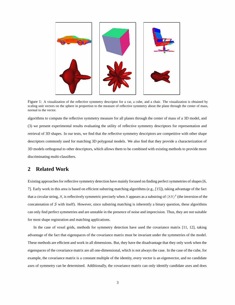
Figure 1: A visualization of the reflective symmetry descriptor for a car, a cube, and a chair. The visualization is obtained byscaling unit vectors on the sphere in proportion to the measure of reflective symmetry about the plane through the center of mass,normal to the vector.

algorithms to compute the reflective symmetry measure for all planes through the center of mass of a 3D model, and

(3) we present experimental results evaluating the utility of reflective symmetry descriptors for representation and

retrieval of 3D shapes. In our tests, we find that the reflective symmetry descriptors are competitive with other shape

descriptors commonly used for matching 3D polygonal models. We also find that they provide a characterization of

3D models orthogonal to other descriptors, which allows them to be combined with existing methods to provide more

discriminating multi-classifiers.

2 Related Work

Existing approaches for reflective symmetry detection have mainly focused on finding perfect symmetries of shapes [6,

7]. Early work in this area is based on efficient substring matching algorithms (e.g., [15]), taking advantage of the fact

that a circular string, S, is reflectively symmetric precisely when S appears as a substring of (SS) t (the inversion of the

concatenation of S with itself). However, since substring matching is inherently a binary question, these algorithms

can only find perfect symmetries and are unstable in the presence of noise and imprecision. Thus, they are not suitable

for most shape registration and matching applications.

In the case of voxel grids, methods for symmetry detection have used the covariance matrix [11, 12], taking

advantage of the fact that eigenspaces of the covariance matrix must be invariant under the symmetries of the model.

These methods are efficient and work in all dimensions. But, they have the disadvantage that they only work when the

eigenspaces of the covariance matrix are all one-dimensional, which is not always the case. In the case of the cube, for

example, the covariance matrix is a constant multiple of the identity, every vector is an eigenvector, and no candidate

axes of symmetry can be determined. Additionally, the covariance matrix can only identify candidate axes and does

3

not determine a measure of symmetry. So, further evaluation needs to be performed to establish the quality of these

candidates as axes of symmetry. Methods for symmetry detection in 2D using more complex moments and Fourier

decomposition have also been described [8, 9, 10, 13], though their dependence on the ability to represent an image as

a function on the complex plane makes them difficult to generalize to three-dimensions.

In the work most similar to ours, Marola [8] presents a method for measuring symmetry invariance of 2D images.

However, because of its use of autocorrelation, the method cannot be extended directly to three-dimensional objects. In

related work, Zabrodsky, Peleg and Avnir [2] define a continuous symmetry distance for point sets in any dimension.

However, it relies on the ability to first establish point correspondences, which is generally difficult. Additionally,

while the method provides a way of computing the symmetry distance for an individual plane of reflection, it does not

provide an efficient algorithm for characterizing a shape by its symmetry distances with respect to multiple planes.

Our work differs from previous research on symmetry detection in that we aim to construct a shape descriptor that

can be used for matching, recognition, and classification of 3D shapes. In this respect, our goals are similar to those of

prior work on shape representations for retrieval and analysis (see [16, 17, 18, 19, 20] for surveys). There, the challenge

is to find a shape descriptor that is: (1) quick to compute, (2) concise to store, (3) easy to index, (4) invariant under

similarity transforms, (5) insensitive to noise and small extra features, (6) independent of 3D object representation,

tessellation, or genus, (7) robust to arbitrary topological degeneracies, and (8) discriminating of shape similarities

and differences. Recent approaches have been based on probability distributions (e.g., [21, 22, 23, 24, 25, 26]), part-

based estimation (e.g., [27, 28, 29, 30]), skeletal decomposition (e.g., [31, 32, 33]), and indexing of local features

(e.g., [34, 35]).

Among these existing shape representations, our work is most related to the shape descriptors that map the 3D

shape of an object to a spherical domain. Some examples include Extended Gaussian Images [36], Orientation His-

tograms [10], Spherical Extent Functions [37], and Spherical Attribute Images [38, 39]. However, these prior ap-

proaches map local surface features (surface orientation, curvature, etc.) to points on a sphere, and thus they are

sensitive to noise in 3D surface data. In contrast, our reflective symmetry descriptor maps global features (integrals

over the entire surface) to each point on a sphere, which provides more stability and descriptive power (as is shown

theoretically in Section 8 and empirically in Section 9).

3 Overview of the Approach

Our approach is to represent the shape of a 3D model with a spherical function that associates continuous measures of

reflective invariance of a 3D model with respect to every plane through its center of mass. The potential advantages of

this approach are three-fold. First, it is defined over a canonical 2D domain (the sphere), and thus it provides a common

parameterization for arbitrary 3D models that can be used for alignment and comparison. Second, it characterizes the

4

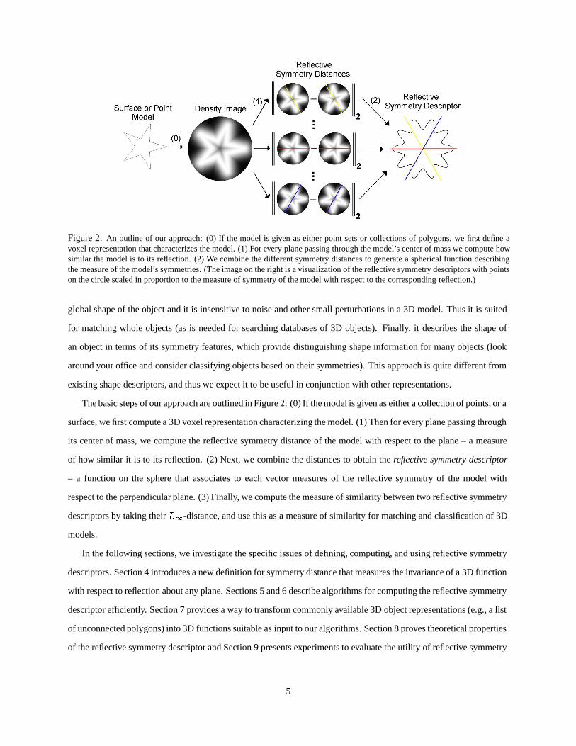
Figure 2: An outline of our approach: (0) If the model is given as either point sets or collections of polygons, we first define avoxel representation that characterizes the model. (1) For every plane passing through the model’s center of mass we compute howsimilar the model is to its reflection. (2) We combine the different symmetry distances to generate a spherical function describingthe measure of the model’s symmetries. (The image on the right is a visualization of the reflective symmetry descriptors with pointson the circle scaled in proportion to the measure of symmetry of the model with respect to the corresponding reflection.)

global shape of the object and it is insensitive to noise and other small perturbations in a 3D model. Thus it is suited

for matching whole objects (as is needed for searching databases of 3D objects). Finally, it describes the shape of

an object in terms of its symmetry features, which provide distinguishing shape information for many objects (look

around your office and consider classifying objects based on their symmetries). This approach is quite different from

existing shape descriptors, and thus we expect it to be useful in conjunction with other representations.

The basic steps of our approach are outlined in Figure 2: (0) If the model is given as either a collection of points, or a

surface, we first compute a 3D voxel representation characterizing the model. (1) Then for every plane passing through

its center of mass, we compute the reflective symmetry distance of the model with respect to the plane – a measure

of how similar it is to its reflection. (2) Next, we combine the distances to obtain the reflective symmetry descriptor

– a function on the sphere that associates to each vector measures of the reflective symmetry of the model with

respect to the perpendicular plane. (3) Finally, we compute the measure of similarity between two reflective symmetry

descriptors by taking their L1-distance, and use this as a measure of similarity for matching and classification of 3D

models.

In the following sections, we investigate the specific issues of defining, computing, and using reflective symmetry

descriptors. Section 4 introduces a new definition for symmetry distance that measures the invariance of a 3D function

with respect to reflection about any plane. Sections 5 and 6 describe algorithms for computing the reflective symmetry

descriptor efficiently. Section 7 provides a way to transform commonly available 3D object representations (e.g., a list

of unconnected polygons) into 3D functions suitable as input to our algorithms. Section 8 proves theoretical properties

of the reflective symmetry descriptor and Section 9 presents experiments to evaluate the utility of reflective symmetry

5

descriptors in practice. Finally, Section 10 contains a brief summary and a dissussion of topics for future work.

4 Definition of the Symmetry Distance

The first issue we must address is to define a measure of symmetry for a 3D model with respect to a plane. While

previous work has proposed symmetry measures for 2D images and 3D point sets [6, 7, 2], we seek such a measure

for arbitrary 3D functions (e.g., represented on voxel grids). In this section, we show that the measure of a function’s

reflective symmetry can be defined as the L2-difference between the model and its reflection (up to scale factor).

The specific contribution is our description of the symmetry distance as the length of a projection onto a subspace of

functions. This interpretation allows us to prove valuable properties of reflective symmetry descriptors in Section 8.

We define the symmetry distance of a function with respect to a given plane of reflection as the L 2-distance to the

nearest function that is invariant with respect to the reflection. More formally, for a function f and a reflection we

write the symmetry distance (SD) as:

SD(f; ) = mingj (g)=g

kf � gk:

Using the facts that the space of functions is an inner product space and that the functions that are invariant to

reflection about define a vector subspace, it follows that the nearest invariant function g is precisely the projection

of f onto the subspace of invariant functions. That is, if we define � to be the projection onto the space of functions

invariant under the action of and we define �? to be the projection onto the orthogonal subspace then:

SD(f; ) = kf � � (f)k = k�? (f)k

so that the symmetry distance of f with respect to is the length of the projection of f onto a subspace of functions

indexed by .

In order to compute an explicit formulation of the projection of f onto the space functions invariant under the

action of , we observe that reflections are orthogonal transformations (that is, they preserve the inner product defined

on the space of functions). This observation lets us apply a theorem from representation theory [44] stating that a

projection of a vector onto the subspace invariant under the action of an orthogonal group is the average of the vector

over the different elements in the group. Thus in the case of a function f and a reflection we get:

SD(f; ) =

f � 1

2(f + (f))

=

f � (f)

2

(1)

so that up to a scale factor the symmetry distance is simply the L2-difference between the initial function and its

reflection.

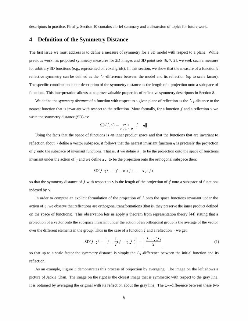
As an example, Figure 3 demonstrates this process of projection by averaging. The image on the left shows a

picture of Jackie Chan. The image on the right is the closest image that is symmetric with respect to the gray line.

It is obtained by averaging the original with its reflection about the gray line. The L 2-difference between these two

6

images is the measure of the symmetry of the initial image with respect to reflection about the gray line. Equivalently,

according to Equation 1, the symmetry distance is half the L 2-distance from the original image to its reflection.

Figure 3: An image of Jackie Chan (left) and its projection onto the space of images invariant under reflection through the grayline (right). The image on the right is obtained by averaging the image on the left with its reflection about the gray line.

5 Computation of the Reflective Symmetry Descriptor

Given a 3D function f , we define its reflective symmetry descriptor as a 2D function on the space of planes through

the origin (indexed by their unit normals), describing the proportion of f that is symmetric with respect to reflection

about a given plane and the proportion of f that is anti-symmetric:

RSD(f; s) =

�k�s(f)kkfk ;

k�?s (f)kkfk

�=

0@qkfk2 � SD2(f; s)

kfk ;SD(f; s)

kfk

1A

where �s is the projection onto the space of functions invariant under reflection about the plane passing through the

origin, perpendicular to s, and �?s is the projection onto the orthogonal complement.

To compute the reflective symmetry descriptor of a 3D model, we first convert it into a density function sampled

on a 3D voxel grid (as described in Section 7). This allows us to leverage the Fast Fourier Transform to compute

the reflective symmetry descriptor in O(N 4 logN) time for an N � N � N voxel grid and a good multiresolution

approximation in O(N 3 logN) time (as described in Section 6). This provides a substantial improvement over the

brute force O(N 5) algorithm, which performs O(N 3) computations for each of O(N 2) planes.

In the following subsections, we describe how to compute the reflective symmetry descriptor efficiently by showing

that the symmetry distances for all planes passing through the origin can be computed without explicitly computing

the reflection of the function about every plane. First, we show how the Fast Fourier Transform can be used to compute

the symmetry distances of a function defined on the boundary of a circle (Section 5.1). Second, we show how the case

of a function f defined on the interior of a unit disk can be reduced to the case of a function on a circle by decomposing

f into a collection of functions defined on concentric circles (Section 5.2). Third, through a collection of mappings

we show how to reduce the question of finding the symmetry distances of a function on the surface of a sphere to the

7

question of finding the symmetry distances of a function on a disk (Section 5.3). Finally, we show how the symmetry

distances of a 3D function represented as a voxel grid can be computed by decomposing the grid into a collection of

concentric spheres and applying the methods for computing the symmetry distances on a sphere (Section 5.4).

5.1 Functions on a Circle

We begin our discussion by looking at functions on the boundary of a circle. For a given function f(�) on the circle

and all reflections we would like to compute the measure of invariance of f with respect to . Denoting by � the

reflection about the line through the origin with angle � and using the fact that this reflection maps a point with angle

� to the point with angle 2�� � (see Figure 4) we can apply Equation 1 to obtain:

SD(f; �) =

sZ 2�

0

�f(�)� f(2�� �)

2

�2

d� =

vuuuutL2-normz }| {kfk22

�

convolution termz }| {Z 2�

0

f(�)f(2�� �)

2d�

This formulation provides an efficient method for computing all the symmetry distances of a function defined on a

unit circle because we can use the Fast Fourier Transform to compute the value of the convolution term for all angles

� in O(N log(N)) time, where N represents the number of times f is sampled on the circle.

Figure 4: Reflection about � maps a point with angle � to the point with angle 2�� �.

5.2 Functions on a Disk

As with functions on a circle, we would like to compute the symmetry distances of a function on the interior of a disk

with respect to all reflections about lines through the origin. To compute the symmetry distances, we observe that

these reflections fix circles of constant radius, and hence the symmetries of a function defined on a disk can be studied

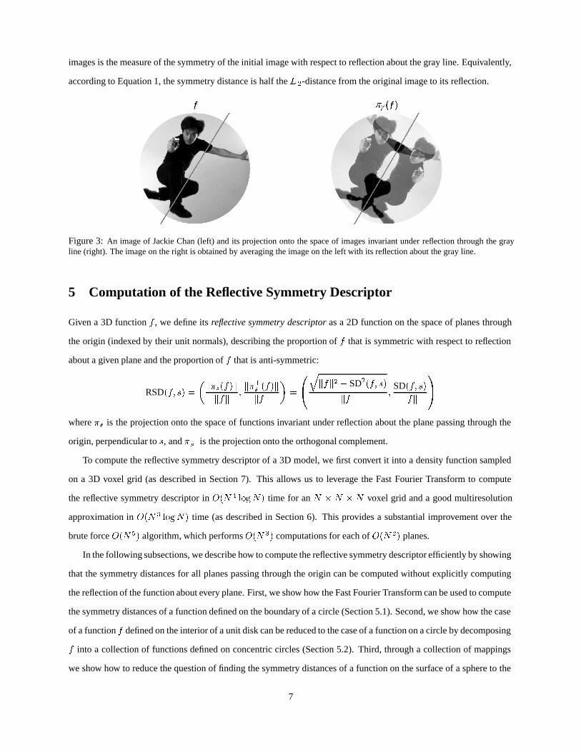
by looking at the restriction of the function to concentric circles. Figure 5 shows a visualization of this process: the

image of Superman is decomposed into concentric circles, and the symmetry distances of the image are computed by

combining the symmetry distances of the different circular functions.

8

Figure 5: The symmetry distances of a 2D image can be obtained by decomposing the image into concentric circles and computingall the symmetry distances for each of the circles.

To make this observation explicit we reparameterize the function f(x; y) into polar coordinates to get the collection

of functions f ~frg with:

~fr(�) = f(r cos �; r sin �);

where r 2 [0; 1] and � 2 [0; 2�], and we set � to be the reflection about the line through the origin with angle �.

Using Equation 1 and applying the appropriate change of variables we get:

SD(f; �) =

sZ 1

0

SD2( ~fr; �)rdr

showing that we can take advantage of the efficient method for computing the symmetry distances of a function on the

circle to obtain an O(N 2 logN) algorithm for computing the symmetry distances of an N �N image.

This method is similar to the method presented in the works of Marola and Sun et al. [8, 10] in its use of au-

tocorrelation as a tool for reflective symmetry detection. The advantage of our formulation is that it describes the

relationship between autocorrelation and an explicit notion of symmetry distance, defined by the L 2 inner-product of

the underlying space of functions, and provides a method for generalizing the definition of symmetry distance to 3D.

5.3 Functions on a Sphere

Next, we look at functions on the surface of a sphere. To compute the reflective symmetry distances of a function on a

sphere, for all planes passing through the origin, we fix a North pole and restrict our attention to those planes passing

through it. The symmetry distances of the restricted set of reflections can be efficiently computed by breaking up

the function into its restrictions to the upper and lower hemisphere and projecting each of these restrictions to a disk.

Figure 6(left) shows a visualization of this process for the restriction to the upper hemisphere. Note that reflections

through planes containing the North pole map the upper hemisphere to itself and correspond to reflections about lines

in the projected function.

In particular if we parameterize the sphere in terms of spherical coordinates:

�(�; �) =�cos�; sin � cos �; sin� sin �

�9

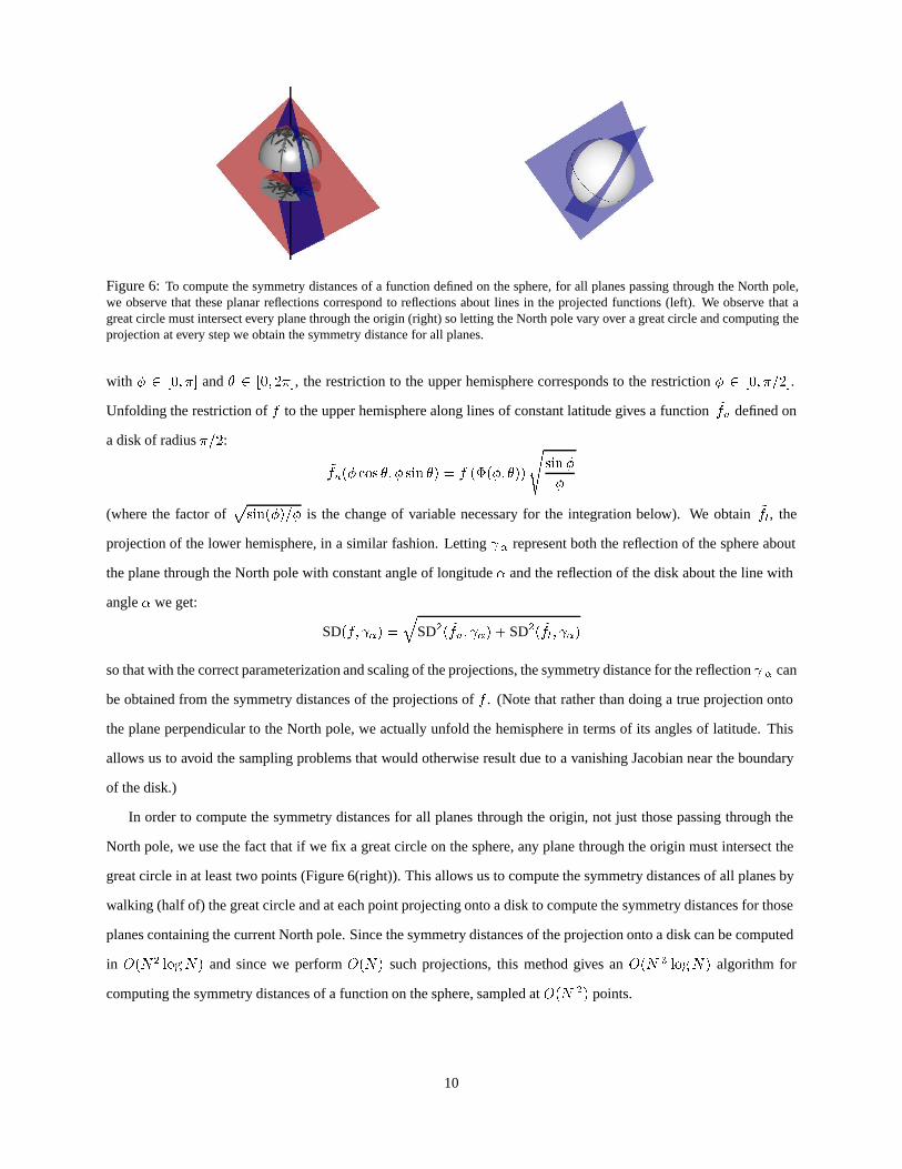
Figure 6: To compute the symmetry distances of a function defined on the sphere, for all planes passing through the North pole,we observe that these planar reflections correspond to reflections about lines in the projected functions (left). We observe that agreat circle must intersect every plane through the origin (right) so letting the North pole vary over a great circle and computing theprojection at every step we obtain the symmetry distance for all planes.

with � 2 [0; �] and � 2 [0; 2�], the restriction to the upper hemisphere corresponds to the restriction � 2 [0; �=2].

Unfolding the restriction of f to the upper hemisphere along lines of constant latitude gives a function ~fu defined on

a disk of radius �=2:

~fu(� cos �; � sin �) = f (�(�; �))

ssin�

�

(where the factor ofpsin(�)=� is the change of variable necessary for the integration below). We obtain ~fl, the

projection of the lower hemisphere, in a similar fashion. Letting � represent both the reflection of the sphere about

the plane through the North pole with constant angle of longitude � and the reflection of the disk about the line with

angle � we get:

SD(f; �) =

qSD2( ~fu; �) + SD2( ~fl; �)

so that with the correct parameterization and scaling of the projections, the symmetry distance for the reflection � can

be obtained from the symmetry distances of the projections of f . (Note that rather than doing a true projection onto

the plane perpendicular to the North pole, we actually unfold the hemisphere in terms of its angles of latitude. This

allows us to avoid the sampling problems that would otherwise result due to a vanishing Jacobian near the boundary

of the disk.)

In order to compute the symmetry distances for all planes through the origin, not just those passing through the

North pole, we use the fact that if we fix a great circle on the sphere, any plane through the origin must intersect the

great circle in at least two points (Figure 6(right)). This allows us to compute the symmetry distances of all planes by

walking (half of) the great circle and at each point projecting onto a disk to compute the symmetry distances for those

planes containing the current North pole. Since the symmetry distances of the projection onto a disk can be computed

in O(N2 logN) and since we perform O(N) such projections, this method gives an O(N 3 logN) algorithm for

computing the symmetry distances of a function on the sphere, sampled at O(N 2) points.

10

5.4 Functions on a Voxel Grid

Finally, we address the problem of computing symmetry distances on a regular N � N � N voxel grid. As in

Section 5.2, we can use the fact that reflections fix lengths to transform this problem into a problem of computing the

symmetry distances of a collection of functions defined on concentric spheres. In particular, if f is a function defined

in the interior of a unit ball, then we decompose f into a collection of functions f ~frg where ~fr is a function defined

on the unit sphere and ~fr(v) = f(rv). After changing variables, the measure of symmetry of f with respect to a

reflection becomes:

SD(f; ) =

sZ 1

0

SD2( ~fr; )r2dr

and we obtain the value of the symmetry descriptor of f as a combination of the values of the symmetry descriptors

of the functions f ~frg defined on the sphere, giving an O(N 4 logN) algorithm for computing the symmetry distances

of an N �N �N voxel model.

6 Multiresolution Approximation

Our algorithm for computing the symmetry distances takes O(N 4 logN) time at full resolution. However, using

Fourier decomposition of the restriction of the function to rays through the origin, we are able to compute a good mul-

tiresolution approximation inO(N 3 logN) time. This approximation is useful in most applications because symmetry

describes global features of a model and is apparent even at low resolutions.

Given a function f defined on the set of points with radius less than or equal to 1 we decompose f into the

collection of one-dimensional functions by fixing rays through the origin and consider the restriction of f to these

rays. This gives a collection of functions f ~fvg, indexed by unit vectors v, with ~fv(t) = f(tv)t and t 2 [0; 1] (where

the factor of t is the change of variable necessary for integration below). Expanding the functions ~fv in terms of their

trigonometric series we get:

~fv(t) = a0(v) +

1Xk=1

�ak(v)

cos(2k�t)p2

+ bk(v)sin(2k�t)p

2

�:

The advantage of this decomposition is that the functions ak(v) and bk(v) are functions defined on the sphere, provid-

ing a multiresolution description of the initial function f . Applying the appropriate change of variables and letting

denote a reflection about a plane through the origin we get:

SD(f; ) =

vuutSD2(a0; ) +1Xk=1

�SD2(ak; ) + SD2(bk; )

�:

Thus a lower bound approximation to the symmetry distances can be obtained in O(N 3 logN) time by only using the

first few of the Fourier coefficient functions ak and bk.

11

7 Voxelization of 3D Models

Our algorithm for computing a reflective symmetry descriptor takes a voxel model as its input. In order to be able to

use it for a general class of shapes, (and not just density images or models with a well defined interior and exterior), it

is first necessary to be able to transform an arbitrary 3D model into a 3D function sampled on a regular voxel grid.

Since we compute the symmetry distance by comparing the initial model with its reflection, we choose a voxel

representation that describes not only where the points on the model are, but also how far an arbitrary point is from

the model. Furthermore, the values of the voxel grid should fall off to zero for voxels further from the model, allowing

us to treat the voxel grid as a sampling of a compactly supported function and to restrict the domain over which we

integrate. To address these issues we define the voxel grid as a sampling of an exponentially decaying Euclidean

Distance Transform. In particular, given a model S we define the implicit function F S by:

FS(x) = exp

��D2

S(x)

R2S

�(2)

where DS(x) is the Euclidean Distance Transform, giving the distance from x to the nearest point on the model S:

DS(x) = miny2S

kx� yk;

and RS is the average distance from a point on S to the center of mass.

In practice, we compute the implicit function FS(x) by first rasterizing the triangles, line segments, or points of a

3D model into an N �N �N voxel grid and then applying the O(N 3) algorithm of Saito et al.[45] to compute the

exponentially decaying distance transform.

The advantage of using this distance function representation is that it allows us to compute the reflective symmetry

descriptor for a wide class of models, including models that are not topologically consistent, models that have cracks,

and models that have flipped triangles. Figure 7 shows fifteen models (above) with their corresponding reflective

symmetry descriptors (underneath). The descriptors were computed without first reconstructing a solid representation

or manifold surface. Note also that the descriptors vary from model to model, with different patterns of undulations

and sharp peaks, demonstrating that the symmetry descriptor is a rich function, capable of describing large amounts

of information about shape.

12

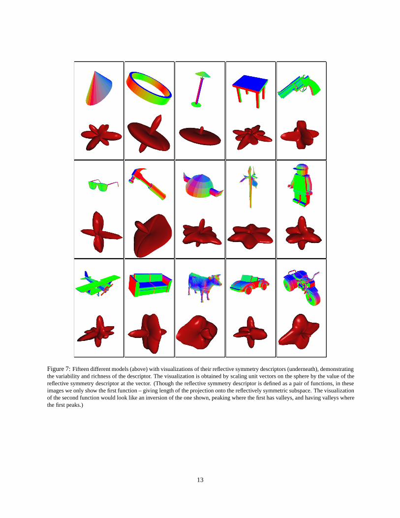
Figure 7: Fifteen different models (above) with visualizations of their reflective symmetry descriptors (underneath), demonstratingthe variability and richness of the descriptor. The visualization is obtained by scaling unit vectors on the sphere by the value of thereflective symmetry descriptor at the vector. (Though the reflective symmetry descriptor is defined as a pair of functions, in theseimages we only show the first function – giving length of the projection onto the reflectively symmetric subspace. The visualizationof the second function would look like an inversion of the one shown, peaking where the first has valleys, and having valleys wherethe first peaks.)

13

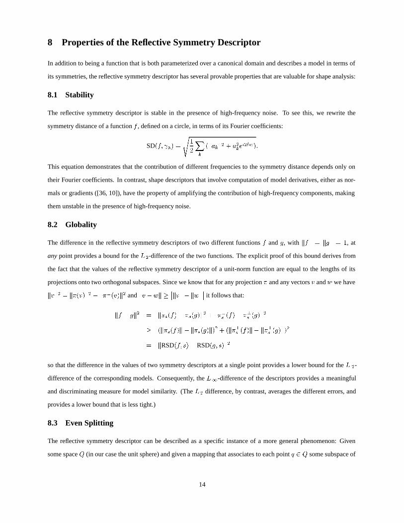
8 Properties of the Reflective Symmetry Descriptor

In addition to being a function that is both parameterized over a canonical domain and describes a model in terms of

its symmetries, the reflective symmetry descriptor has several provable properties that are valuable for shape analysis:

8.1 Stability

The reflective symmetry descriptor is stable in the presence of high-frequency noise. To see this, we rewrite the

symmetry distance of a function f , defined on a circle, in terms of its Fourier coefficients:

SD(f; �) =

s1

2

Xk

(kakk2 + a2kei2k�):

This equation demonstrates that the contribution of different frequencies to the symmetry distance depends only on

their Fourier coefficients. In contrast, shape descriptors that involve computation of model derivatives, either as nor-

mals or gradients ([36, 10]), have the property of amplifying the contribution of high-frequency components, making

them unstable in the presence of high-frequency noise.

8.2 Globality

The difference in the reflective symmetry descriptors of two different functions f and g, with kfk = kgk = 1, at

any point provides a bound for the L2-difference of the two functions. The explicit proof of this bound derives from

the fact that the values of the reflective symmetry descriptor of a unit-norm function are equal to the lengths of its

projections onto two orthogonal subspaces. Since we know that for any projection � and any vectors v and w we have

kvk2 = k�(v)k2 + k�?(v)k2 and kv � wk ���kvk � kwk

�� it follows that:

kf � gk2 = k�s(f)� �s(g)k2 + k�?s (f)� �?s (g)k2

� (k�s(f)k � k�s(g)k)2 + (k�?s (f)k � k�?s (g)k)2

= kRSD(f; s)� RSD(g; s)k2

so that the difference in the values of two symmetry descriptors at a single point provides a lower bound for the L 2-

difference of the corresponding models. Consequently, the L1-difference of the descriptors provides a meaningful

and discriminating measure for model similarity. (The L2 difference, by contrast, averages the different errors, and

provides a lower bound that is less tight.)

8.3 Even Splitting

The reflective symmetry descriptor can be described as a specific instance of a more general phenomenon: Given

some space Q (in our case the unit sphere) and given a mapping that associates to each point q 2 Q some subspace of

14

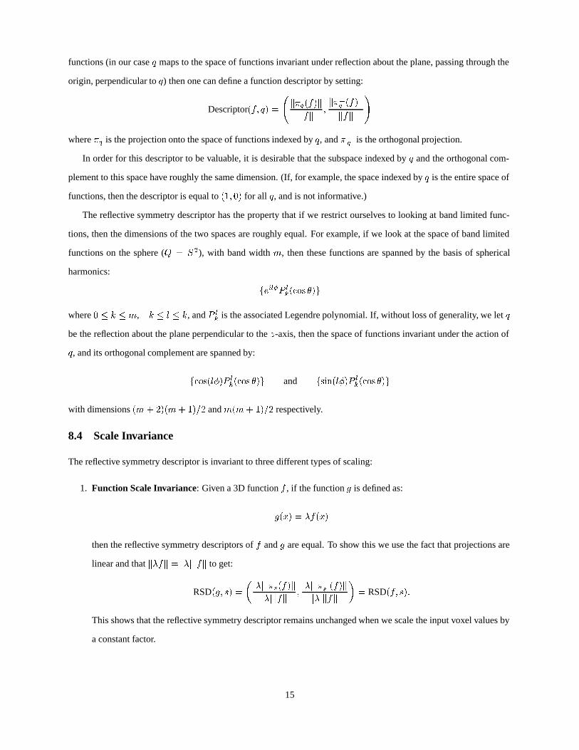
functions (in our case q maps to the space of functions invariant under reflection about the plane, passing through the

origin, perpendicular to q) then one can define a function descriptor by setting:

Descriptor(f; q) =

k�q(f)kkfk ;

k�?q (f)kkfk

!

where �q is the projection onto the space of functions indexed by q, and �?q is the orthogonal projection.

In order for this descriptor to be valuable, it is desirable that the subspace indexed by q and the orthogonal com-

plement to this space have roughly the same dimension. (If, for example, the space indexed by q is the entire space of

functions, then the descriptor is equal to (1; 0) for all q, and is not informative.)

The reflective symmetry descriptor has the property that if we restrict ourselves to looking at band limited func-

tions, then the dimensions of the two spaces are roughly equal. For example, if we look at the space of band limited

functions on the sphere (Q = S 2), with band width m, then these functions are spanned by the basis of spherical

harmonics:

feil�P lk(cos �)g

where 0 � k � m, �k � l � k, and P lk is the associated Legendre polynomial. If, without loss of generality, we let q

be the reflection about the plane perpendicular to the z-axis, then the space of functions invariant under the action of

q, and its orthogonal complement are spanned by:

fcos(l�)P lk(cos �)g and fsin(l�)P l

k(cos �)g

with dimensions (m+ 2)(m+ 1)=2 and m(m+ 1)=2 respectively.

8.4 Scale Invariance

The reflective symmetry descriptor is invariant to three different types of scaling:

1. Function Scale Invariance: Given a 3D function f , if the function g is defined as:

g(x) = �f(x)

then the reflective symmetry descriptors of f and g are equal. To show this we use the fact that projections are

linear and that k�fk = j�jkfk to get:

RSD(g; s) =

� j�jk�s(f)kj�jkfk ;

j�jk�?s (f)kj�jkfk

�= RSD(f; s):

This shows that the reflective symmetry descriptor remains unchanged when we scale the input voxel values by

a constant factor.

15

2. Domain Scale Invariance: Given a 3D function f , if the function g is defined as:

g(x) = f(�x)

then the reflective symmetry descriptors of f and g are equal. To show this we note that if is a reflection about

any plane through the origin and ~f = � (f) is the projection of f onto the space of functions invariant under

reflection by , then ~f is the nearest -invariant function to f . Since it is also true that ~f(�x) is -invariant, it

follows that:

k�? (g)k � kg(x)� ~f(�x)k = kf(�x)� ~f(�x)gk = k�? (f)kj�j3 :

Similarly, we can reverse the argument to get:

k�? (g)k �k�? (f)kj�j3 :

Thus, we get:

RSD(g; s) =

� j�j3k�s(f)kj�j3kfk ;

j�j3k�?s (f)kj�j3kfk

�= RSD(f; s)

This shows that the reflective symmetry descriptor is independent of the resolution of the input voxel grid.

3. Model Scale Invariance: Given a 3D shape S, if the shape T is obtained by scaling S by �, T = �S, then the

reflective symmetry descriptors of S and T are equal. To show this we first recall that the implicit function used

for computing the reflective symmetry descriptor of S is defined as:

FS(x) = exp(�D2S(x)=R

2S);

where DS(x) is the Euclidean distance transform of S, and RS is the average distance from points on S to the

center of mass. Using the fact that RT = �RS , and using the fact that:

DT (x) = �DS(x=�)

we get:

FT (x) = exp

��D2

T (x)

R2T

�= exp

���2D2

S(x=�)

�2R2S

�= FS(x=�):

Thus, from the domain scale invariance property, it follows that the reflective symmetry descriptors of S and T

are equal – i.e., the reflective symmetry descriptor is independent of the scale of the input 3D model.

16

9 Experimental Results

While the properties described in Section 8 indicate that the reflective symmetry descriptor may be well suited for

shape analysis tasks in theory, it is necessary to demonstrate that these properties translate into desirable properties in

practice. This section presents experiments used to investigate the following questions:

� How stable is the descriptor if noise is added to the model?

� How robust is the descriptor with respect to point sampling?

� How quickly does the multiresolution approximation converge to the descriptor?

� How well does the descriptor classify models?

� How orthogonal is the reflective symmetry descriptor to other descriptors?

For the purposes of these experiments, the reflective symmetry descriptor of a polygonal model was computed by

rasterizing the model into a 64� 64� 64 voxel grid. The models were translated so that the center of mass was at the

center of the voxel grid, and they were rescaled so that the average distance of a point on the model from the center

was one quarter the resolution of the grid (we found that twice the average distance to the center of mass was a more

stable measure of the extent of a model than its bounding radius). The reflective symmetry descriptors were computed

on an 800 MHz Athlon processor with 512 MB of RAM. The polygonal models took between 0:2 and 3:5 seconds to

rasterize for polygon counts ranging from 20 to 120,000; the exponentiated distance transform took 1:2 seconds; and,

the descriptor of the voxel grid took 5 seconds to compute.

9.1 Noise

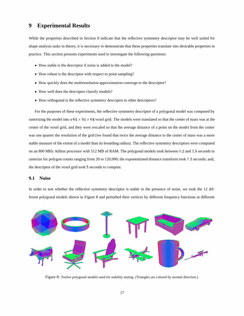
In order to test whether the reflective symmetry descriptor is stable in the presence of noise, we took the 12 dif-

ferent polygonal models shown in Figure 8 and perturbed their vertices by different frequency functions at different

Figure 8: Twelve polygonal models used for stability testing. (Triangles are colored by normal direction.)

17

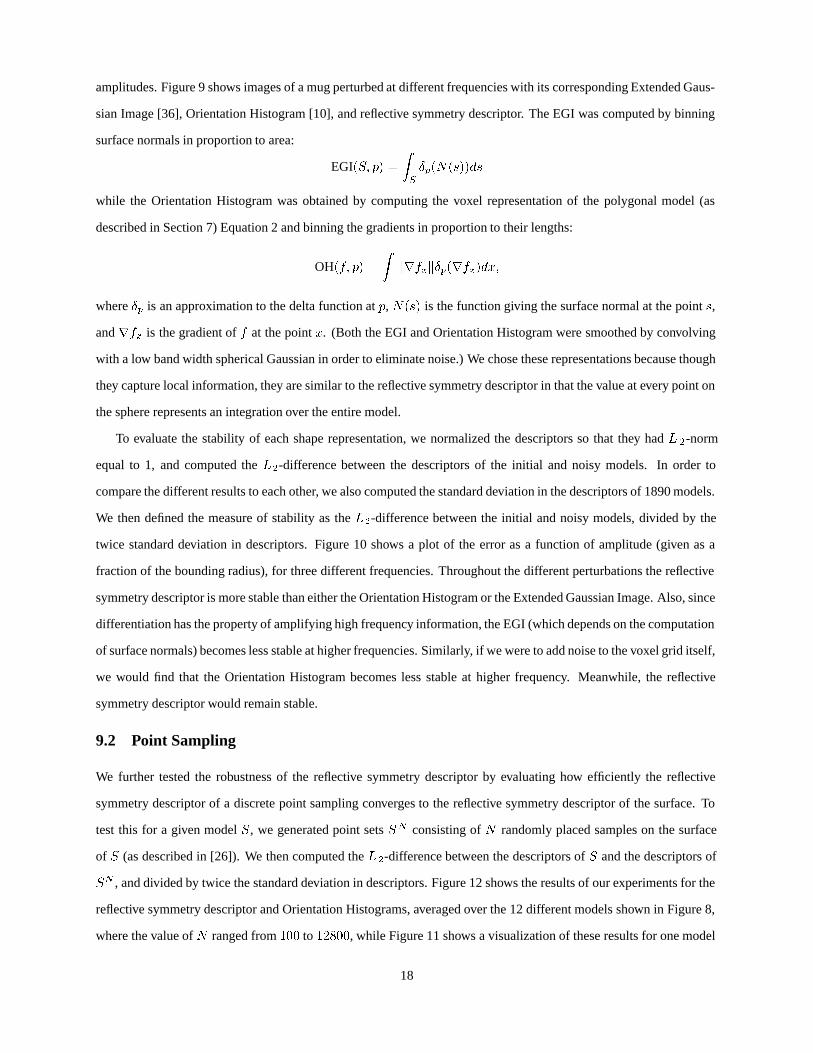
amplitudes. Figure 9 shows images of a mug perturbed at different frequencies with its corresponding Extended Gaus-

sian Image [36], Orientation Histogram [10], and reflective symmetry descriptor. The EGI was computed by binning

surface normals in proportion to area:

EGI(S; p) =ZS

Æp(N(s))ds

while the Orientation Histogram was obtained by computing the voxel representation of the polygonal model (as

described in Section 7) Equation 2 and binning the gradients in proportion to their lengths:

OH(f; p) =

ZkrfxkÆp(rfx)dx;

where Æp is an approximation to the delta function at p, N(s) is the function giving the surface normal at the point s,

and rfx is the gradient of f at the point x. (Both the EGI and Orientation Histogram were smoothed by convolving

with a low band width spherical Gaussian in order to eliminate noise.) We chose these representations because though

they capture local information, they are similar to the reflective symmetry descriptor in that the value at every point on

the sphere represents an integration over the entire model.

To evaluate the stability of each shape representation, we normalized the descriptors so that they had L 2-norm

equal to 1, and computed the L2-difference between the descriptors of the initial and noisy models. In order to

compare the different results to each other, we also computed the standard deviation in the descriptors of 1890 models.

We then defined the measure of stability as the L2-difference between the initial and noisy models, divided by the

twice standard deviation in descriptors. Figure 10 shows a plot of the error as a function of amplitude (given as a

fraction of the bounding radius), for three different frequencies. Throughout the different perturbations the reflective

symmetry descriptor is more stable than either the Orientation Histogram or the Extended Gaussian Image. Also, since

differentiation has the property of amplifying high frequency information, the EGI (which depends on the computation

of surface normals) becomes less stable at higher frequencies. Similarly, if we were to add noise to the voxel grid itself,

we would find that the Orientation Histogram becomes less stable at higher frequency. Meanwhile, the reflective

symmetry descriptor would remain stable.

9.2 Point Sampling

We further tested the robustness of the reflective symmetry descriptor by evaluating how efficiently the reflective

symmetry descriptor of a discrete point sampling converges to the reflective symmetry descriptor of the surface. To

test this for a given model S, we generated point sets SN consisting of N randomly placed samples on the surface

of S (as described in [26]). We then computed the L2-difference between the descriptors of S and the descriptors of

SN , and divided by twice the standard deviation in descriptors. Figure 12 shows the results of our experiments for the

reflective symmetry descriptor and Orientation Histograms, averaged over the 12 different models shown in Figure 8,

where the value of N ranged from 100 to 12800, while Figure 11 shows a visualization of these results for one model

18

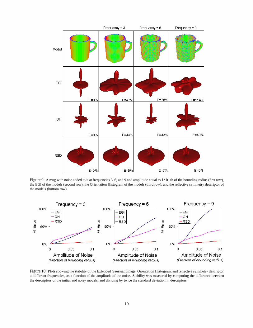
Figure 9: A mug with noise added to it at frequencies 3, 6, and 9 and amplitude equal to 1=10-th of the bounding radius (first row),the EGI of the models (second row), the Orientation Histogram of the models (third row), and the reflective symmetry descriptor ofthe models (bottom row).

Figure 10: Plots showing the stability of the Extended Gaussian Image, Orientation Histogram, and reflective symmetry descriptorat different frequencies, as a function of the amplitude of the noise. Stability was measured by computing the difference betweenthe descriptors of the initial and noisy models, and dividing by twice the standard deviation in descriptors.

19

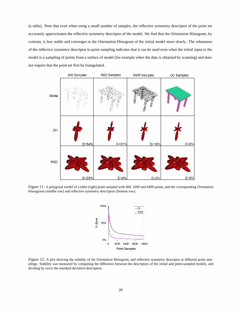
(a table). Note that even when using a small number of samples, the reflective symmetry descriptor of the point set

accurately approximates the reflective symmetry descriptor of the model. We find that the Orientation Histogram, by

contrast, is less stable and converges to the Orientation Histogram of the initial model more slowly. The robustness

of the reflective symmetry descriptor to point sampling indicates that it can be used even when the initial input to the

model is a sampling of points from a surface of model (for example when the data is obtained by scanning) and does

not require that the point set first be triangulated.

Figure 11: A polygonal model of a table (right) point sampled with 400, 1600 and 6400 points, and the corresponding OrientationHistograms (middle row) and reflective symmetry descriptors (bottom row).

Figure 12: A plot showing the stability of the Orientation Histogram, and reflective symmetry descriptor at different point sam-plings. Stability was measured by computing the difference between the descriptors of the initial and point-sampled models, anddividing by twice the standard deviation descriptors.

20

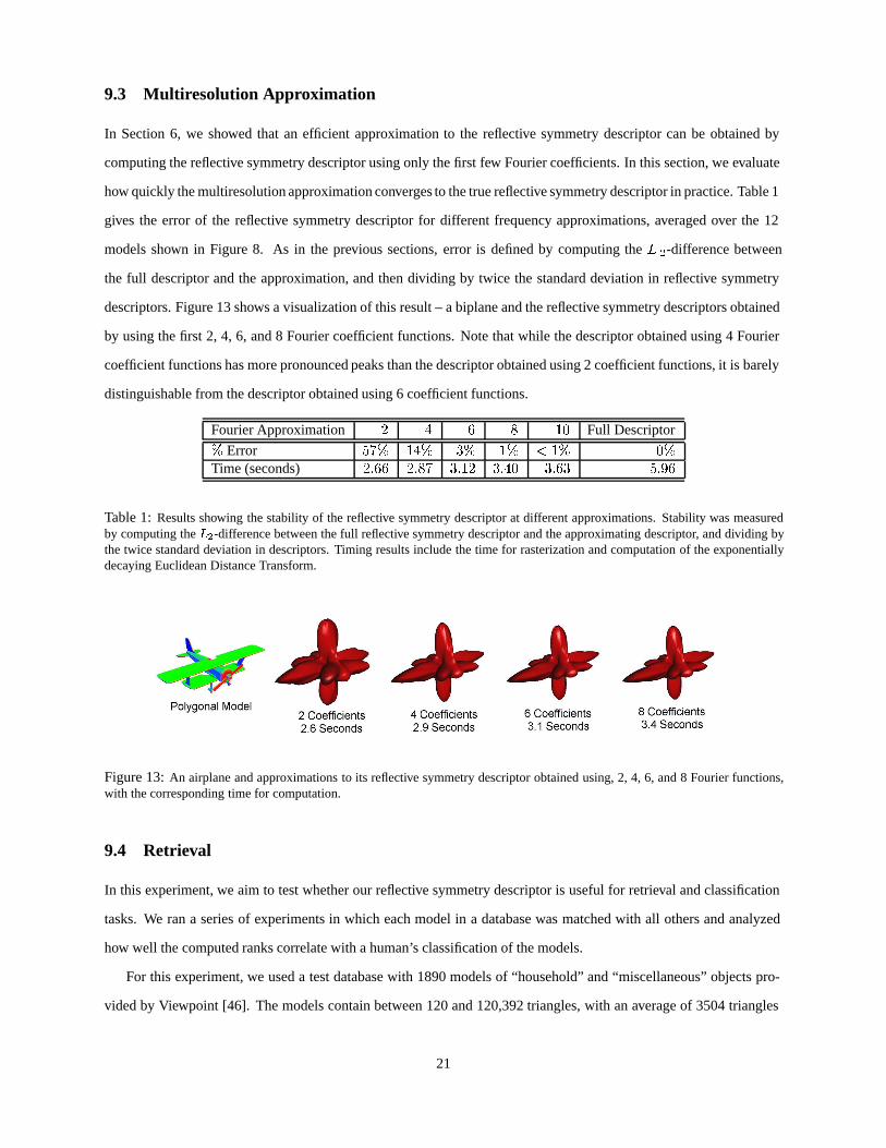
9.3 Multiresolution Approximation

In Section 6, we showed that an efficient approximation to the reflective symmetry descriptor can be obtained by

computing the reflective symmetry descriptor using only the first few Fourier coefficients. In this section, we evaluate

how quickly the multiresolution approximation converges to the true reflective symmetry descriptor in practice. Table 1

gives the error of the reflective symmetry descriptor for different frequency approximations, averaged over the 12

models shown in Figure 8. As in the previous sections, error is defined by computing the L 2-difference between

the full descriptor and the approximation, and then dividing by twice the standard deviation in reflective symmetry

descriptors. Figure 13 shows a visualization of this result – a biplane and the reflective symmetry descriptors obtained

by using the first 2, 4, 6, and 8 Fourier coefficient functions. Note that while the descriptor obtained using 4 Fourier

coefficient functions has more pronounced peaks than the descriptor obtained using 2 coefficient functions, it is barely

distinguishable from the descriptor obtained using 6 coefficient functions.

Fourier Approximation 2 4 6 8 10 Full Descriptor

% Error 57% 14% 3% 1% < 1% 0%Time (seconds) 2:66 2:87 3:12 3:40 3:63 5:96

Table 1: Results showing the stability of the reflective symmetry descriptor at different approximations. Stability was measuredby computing the L2-difference between the full reflective symmetry descriptor and the approximating descriptor, and dividing bythe twice standard deviation in descriptors. Timing results include the time for rasterization and computation of the exponentiallydecaying Euclidean Distance Transform.

Figure 13: An airplane and approximations to its reflective symmetry descriptor obtained using, 2, 4, 6, and 8 Fourier functions,with the corresponding time for computation.

9.4 Retrieval

In this experiment, we aim to test whether our reflective symmetry descriptor is useful for retrieval and classification

tasks. We ran a series of experiments in which each model in a database was matched with all others and analyzed

how well the computed ranks correlate with a human’s classification of the models.

For this experiment, we used a test database with 1890 models of “household” and “miscellaneous” objects pro-

vided by Viewpoint [46]. The models contain between 120 and 120,392 triangles, with an average of 3504 triangles

21

per object. Models were clustered into 85 classes based on functional similarities, largely following the grouping

provided by Viewpoint. The smallest class had 5 models, the largest had 153 models, and 610 models did not fit into

any meaningful class. Examples of ten different classes are shown in Figure 14.

We chose this database for our tests because it provides a representative repository of 3D polygonal models, and

it is difficult for shape-based retrieval. In particular, several distinct classes contain models with very similar shapes.

For example, there are five separate classes of chairs (153 dining room chairs, 10 desk chairs, 5 director chairs, 25

living room chairs, and 6 lounge chairs). Meanwhile, there are classes spanning a wide variety of shapes (e.g., plates

of food, bottles, etc.). Thus, the database stresses the discrimination power of our reflective symmetry descriptor while

testing it under a variety of conditions. Furthermore, since the models were consistently aligned by Viewpoint in a

common coordinate frame, we were able to test the discriminatory power of different shape descriptors independent

of an automatic alignment method (e.g., principal axes).

153 dining room chairs 25 living room chairs 8 chests 16 beds 12 dining tables

36 end tables 39 vases 28 bottles 9 chandeliers 5 candelabra

Figure 14: Samples from ten representative classes from the Viewpoint “household” and “miscellaneous” database (images cour-tesy of Viewpoint [46]).

In this experiment, we compared the retrieval results of seven alignment-dependent shape matching methods:

� RSD1: L1-difference of the reflective symmetry descriptors

� RSD2: L2-difference of the reflective symmetry descriptors

� EGI: L2-difference of the Extended Gaussian Images, as computed in [36]

� OH: L2-difference of the Orientation Histograms, as computed in [10]

� EXT: L2-difference of the Spherical Extent Functions, as computed in [37]

� MOM: L2-difference of the moments up to order 7, as computed in [47]

� VOXEL: L2-difference of the voxel model, as described in Section 7 Equation 2

22

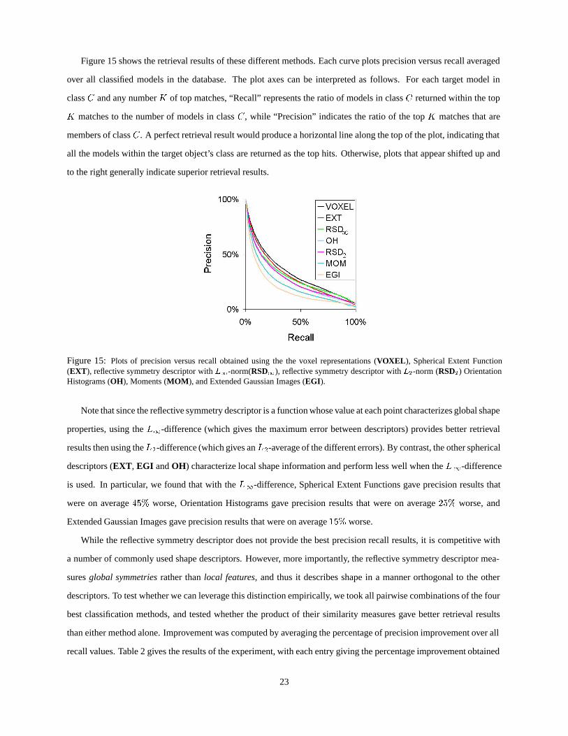
Figure 15 shows the retrieval results of these different methods. Each curve plots precision versus recall averaged

over all classified models in the database. The plot axes can be interpreted as follows. For each target model in

class C and any number K of top matches, “Recall” represents the ratio of models in class C returned within the top

K matches to the number of models in class C, while “Precision” indicates the ratio of the top K matches that are

members of class C. A perfect retrieval result would produce a horizontal line along the top of the plot, indicating that

all the models within the target object’s class are returned as the top hits. Otherwise, plots that appear shifted up and

to the right generally indicate superior retrieval results.

Figure 15: Plots of precision versus recall obtained using the the voxel representations (VOXEL), Spherical Extent Function(EXT), reflective symmetry descriptor with L1-norm(RSD1), reflective symmetry descriptor with L2-norm (RSD2) OrientationHistograms (OH), Moments (MOM), and Extended Gaussian Images (EGI).

Note that since the reflective symmetry descriptor is a function whose value at each point characterizes global shape

properties, using the L1-difference (which gives the maximum error between descriptors) provides better retrieval

results then using theL2-difference (which gives anL2-average of the different errors). By contrast, the other spherical

descriptors (EXT, EGI and OH) characterize local shape information and perform less well when the L1-difference

is used. In particular, we found that with the L1-difference, Spherical Extent Functions gave precision results that

were on average 45% worse, Orientation Histograms gave precision results that were on average 25% worse, and

Extended Gaussian Images gave precision results that were on average 15% worse.

While the reflective symmetry descriptor does not provide the best precision recall results, it is competitive with

a number of commonly used shape descriptors. However, more importantly, the reflective symmetry descriptor mea-

sures global symmetries rather than local features, and thus it describes shape in a manner orthogonal to the other

descriptors. To test whether we can leverage this distinction empirically, we took all pairwise combinations of the four

best classification methods, and tested whether the product of their similarity measures gave better retrieval results

than either method alone. Improvement was computed by averaging the percentage of precision improvement over all

recall values. Table 2 gives the results of the experiment, with each entry giving the percentage improvement obtained

23

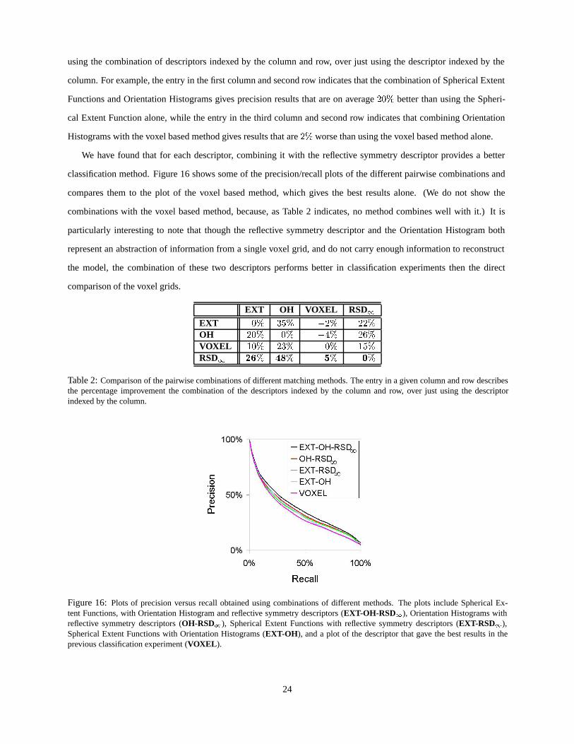
using the combination of descriptors indexed by the column and row, over just using the descriptor indexed by the

column. For example, the entry in the first column and second row indicates that the combination of Spherical Extent

Functions and Orientation Histograms gives precision results that are on average 20% better than using the Spheri-

cal Extent Function alone, while the entry in the third column and second row indicates that combining Orientation

Histograms with the voxel based method gives results that are 2% worse than using the voxel based method alone.

We have found that for each descriptor, combining it with the reflective symmetry descriptor provides a better

classification method. Figure 16 shows some of the precision/recall plots of the different pairwise combinations and

compares them to the plot of the voxel based method, which gives the best results alone. (We do not show the

combinations with the voxel based method, because, as Table 2 indicates, no method combines well with it.) It is

particularly interesting to note that though the reflective symmetry descriptor and the Orientation Histogram both

represent an abstraction of information from a single voxel grid, and do not carry enough information to reconstruct

the model, the combination of these two descriptors performs better in classification experiments then the direct

comparison of the voxel grids.

EXT OH VOXEL RSD1EXT 0% 35% �2% 22%OH 20% 0% �4% 26%VOXEL 10% 23% 0% 15%RSD1 26% 48% 5% 0%

Table 2: Comparison of the pairwise combinations of different matching methods. The entry in a given column and row describesthe percentage improvement the combination of the descriptors indexed by the column and row, over just using the descriptorindexed by the column.

Figure 16: Plots of precision versus recall obtained using combinations of different methods. The plots include Spherical Ex-tent Functions, with Orientation Histogram and reflective symmetry descriptors (EXT-OH-RSD1), Orientation Histograms withreflective symmetry descriptors (OH-RSD1), Spherical Extent Functions with reflective symmetry descriptors (EXT-RSD1),Spherical Extent Functions with Orientation Histograms (EXT-OH), and a plot of the descriptor that gave the best results in theprevious classification experiment (VOXEL).

24

10 Conclusion and Future Work

In this paper, we have introduced the reflective symmetry descriptor, a function associating measures of reflective

invariance of a 3D model with respect to every plane through the center of mass. It has several desirable properties,

including parameterization over a canonical domain, stability, globality, and invariance to scale, that make it useful for

shape analysis tasks. We have shown how to compute it efficiently and conducted experiments that show it is a stable

descriptor that performs well in classification experiments, especially in conjunction with other common descriptors.

This work suggests a number of questions to be addressed in future research: (1) Can the symmetry descriptor

be used for other shape analysis tasks, such as registration and indexing? (2) Can other theoretical properties of the

descriptor be proven, such as showing when 3D models can have the same descriptor? (3) Is the globality property

of the reflective symmetry descriptor sufficiently powerful to allow it to be used with randomized shape analysis

algorithms, (e.g. efficient algorithms that make decisions about alignment and classification by only sparsely sampling

the descriptor)? Answers to these questions will further our understanding of how symmetry defines shape.

References[1] Mitsumoto, H., Tamura, S., Okazaki, K., Kajimi, N., Fukui, Y.: Reconstruction using mirror images based on a plane

symmetry recovery method (1992)

[2] Zabrodsky, H., Peleg, S., Avnir, D.: Symmetry as a continuous feature. IEEE PAMI 17 (1995) 1154–1156

[3] Liu, Y., Rothfus, W., Kanade, T.: Content-based 3d neuroradiologic image retrieval: Preliminary results (1998)

[4] Leou, J., Tsai, W.: Automatic rotational symmetry determination for shape analysis. Pattern Recognition 20 (1987) 571–582

[5] Wolfson, H., Reisfeld, D., Yeshurun, Y.: Robust facial feature detection using symmetry. Proceedings of the InternationalConference on Pattern Recognition (1992) 117–120

[6] Atallah, M.J.: On symmetry detection. IEEE Trans. on Computers c-34 (1985) 663–666

[7] Wolter, J.D., Woo, T.C., Volz, R.A.: Optimal algorithms for symmetry detection in two and three dimensions. The VisualComputer 1 (1985) 37–48

[8] Marola, G.: On the detection of the axes of symmetry of symmetric and almost symmetric planar images. IEEE PAMI 11(1989) 104–108

[9] Shen, D., Ip, H., Cheung, K., Teoh, E.: Symmetry detection by generalized complex (gc) moments: A close-form solution.IEEE PAMI 21 (1999) 466–476

[10] Sun, C., Si, D.: Fast reflectional symmetry detection using orientation histograms. Real-Time Imaging 5 (1999) 63–74

[11] O’Mara, D., Owens, R.: Measuring bilateral symmetry in digital images. IEEE-TENCON - Digital Signal ProcessingApplications (1996)

[12] Sun, C., Sherrah, J.: 3-d symmetry detection using the extended Gaussian image. IEEE PAMI 19 (1997)

[13] Kovesi, P.: Symmetry and asymmetry from local phase. Tenth Australian Joint Converence on Artificial Intelligence (1997)2–4

[14] Kazhdan, M., Chazelle, B., Dobkin, D., Finkelstein, A., Funkhouser, T.: A reflective symmetry descriptor. European Confer-ence on Computer Vision (ECCV) (2002)

[15] Knuth, D., J.H. Morris, J., Pratt, V.: Fast pattern matching in strings. SIAM Journal of Computing 6 (1977) 323–350

[16] Alt, H., Guibas, L.J.: Discrete geometric shapes: Matching, interpolation, and approximation: A survey. Technical Report B96-11, EVL-1996-142, Institute of Computer Science, Freie Universitat Berlin (1996)

[17] Besl, P.J., Jain, R.C.: Three-dimensional object recognition. Computing Surveys 17 (1985) 75–145

[18] Loncaric, S.: A survey of shape analysis techniques. Pattern Recognition 31 (1998) 983–1001

25

[19] Pope, A.R.: Model-based object recognition: A survey of recent research. Technical Report TR-94-04, University of BritishColumbia (1994)

[20] Veltkamp, R.C.: Shape matching: Similarity measures and algorithms. In: Shape Modelling International. (2001) 188–197

[21] Aherne, F., Thacker, N., Rockett, P.: Optimal pairwise geometric histograms. In: Proc. BMVC, Essex, UK (1997) 480–490

[22] Ankerst, M., Kastenmuller, G., Kriegel, H.P., Seidl, T.: 3D shape histograms for similarity search and classification in spatialdatabases. In: Proc. SSD. (1999)

[23] A.P.Ashbrook, N.A.Thacker, P.I.Rockett, C.I.Brown: Robust recognition of scaled shapes using pairwise geometric his-tograms. In: Proc. BMVC, Birmingham, UK (1995) 503–512

[24] Besl, P.: Triangles as a primary representation. Object Recognition in Computer Vision LNCS 994 (1995) 191–206

[25] Evans, A., Thacker, N., Mayhew, J.: Pairwise representation of shape. In: Proc. 11th ICPR. Volume 1., The Hague, theNetherlands (1992) 133–136

[26] Osada, R., Funkhouser, T., Chazelle, B., Dobkin, D.: Matching 3d models with shape distributions. Shape Matching Interna-tional (2001)

[27] Binford, T.: Visual perception by computer. IEEE Conference on Systems Science and Cybernetics (1971)

[28] DeCarlo, D., Metaxas, D., Stone, M.: An anthropometric face model using variational techniques. SIGGRAPH ConferenceProceedings (1998) 67–74

[29] Solina, F., Bajcsy, R.: Recovery of parametric models from range images: The case for superquadrics with global deforma-tions. IEEE Transactions on Pattern Analysis and Machine Intelligence 12 (1990) 131– 147

[30] Wu, K., Levine, M.: Recovering parametric geons from multiview range data. In: Proc. CVPR. (1994) 159–166

[31] Blum, H.: A transformation for extracting new descriptors of shape. In Wathen-Dunn, W., ed.: Proc. Models for the Perceptionof Speech and Visual Form, Cambridge, MA, MIT Press (1967) 362–380

[32] Hilaga, M., Shinagawa, Y., Kohmura, T., Kunii, T.L.: Topology matching for fully automatic similarity estimation of 3Dshapes. Computer Graphics (SIGGRAPH 2001) (2001) 203–212

[33] Siddiqi, K., Shokoufandeh, A., Dickinson, S., Zucker, S.: Shock graphs and shape matching. IJCV 35 (1999) 13–32

[34] Johnson, A.E., Hebert, M.: Using spin-images for efficient multiple model recognition in cluttered 3-D scenes. IEEE PAMI21 (1999) 433–449

[35] Mori, G., Belongie, S., Malik, H.: Shape contexts enable efficient retrieval of similar shapes. CVPR 1 (2001) 723–730

[36] B. Horn, B.: Extended gaussian images. PIEEE 72 (1984) 1656–1678

[37] Vranic, D., Saupe, D.: 3d model retrieval with spherical harmonics and moments. Proceedings of the DAGM (2001) 392–397

[38] Delingette, H., Hebert, M., Ikeuchi, K.: Shape representation and image segmentation using deformable surfaces. Image andVision Computing 10 (1992) 132–144

[39] Delingette, H., Hebert, M., Ikeuchi, K.: A spherical representation for the recognition of curved objects. In: Proc. ICCV.(1993) 103–112

[40] Bloomenthal, J., Lim, C.: Skeletal methods of shape manipulation. Shape Modeling and Applications (1999) 44–47

[41] Storti, D., Turkiyyah, G., Ganter, M., Lim, C., Stal, D.: Skeleton-based modeling operations on solids. Symposium on SolidModeling and Applications (1997) 141–154

[42] Shokoufandeh, A., Dickinson, S.J., Siddiqi, K., Zucker, S.W.: Indexing using a spectral encoding of topological structure. In:Proc. Computer Vision and Pattern Recognition. Volume 2., IEEE (1999) 491–497

[43] Siddiqi, K., Shokoufandeh, A., Dickinson, S., Zucker, S.: Shock graphs and shape matching. Sixth International Conferenceon Computer Vision (1998) 222–229

[44] Serre, J.: Linear Representations of Finite Groups. Springer-Verlag, New York (1977)

[45] Saito, T., Toriwaki, J.: New algorithms for euclidean distance transformation of an n-dimensional digitized picture withapplications. Pattern Recognition 27 (1994) 1551–1565

[46] Labs, V.D.: http://www.viewpoint.com (2001)

[47] Elad, M., Tal, A., Ar, S.: Directed search in a 3d objects database using svm (2000)

26