a reflexive neural network for dynamic biped walking … · a reflexive neural network for...
TRANSCRIPT
A Reflexive Neural Network for DynamicBiped Walking Control
Tao Geng1, Bernd Porr2 Florentin Worgotter1,3
1Department of Psychology, University of Stirling, Stirling, [email protected]
2Department of Electronics & Electrical Eng., University of Glasgow, [email protected]
3Bernstein Center for Computational Neuroscience, University of Gottingen,Germany
All correspondence to:Tao Geng, [email protected]
Abstract
Biped walking remains a difficult problem and robot models can
greatly facilitate our understanding of the underlying biomechanical
principles as well as their neuronal control. The goal of this study is to
specifically demonstrate that stable biped walking can be achieved by
combining the physical properties of the walking robot with a small,
reflex based neuronal network, which is governed mainly by local sen-
sor signals. Building on earlier work (Taga, 1995; Cruse et al., 1998),
this study shows that human-like gaits emerge without specific posi-
tion or trajectory control and that the walker is able to compensate
small disturbances through its own dynamical properties. The re-
flexive controller used here has the following characteristics, which
are different from earlier approaches: (1) Control is mainly local.
Hence, it uses only two signals (AEA=Anterior Extreme Angle and
GC=Ground Contact) which operate at the inter-joint level. All other
signals operate only at single joints. (2) Neither position control nor
trajectory tracking control is used. Instead, the approximate nature
of the local reflexes on each joint allows the robot mechanics itself
(e.g., its passive dynamics) to contribute substantially to the overall
gait trajectory computation. (3) The motor control scheme used in
1

the local reflexes of our robot is more straightforward and has more
biological plausibility than that of other robots, because the outputs
of the motor-neurons in our reflexive controller are directly driving the
motors of the joints, rather than working as references for position or
velocity control. As a consequence, the neural controller and the robot
mechanics are closely coupled as a neuro-mechanical system and this
study emphasizes that dynamically stable biped walking gaits emerge
from the coupling between neural computation and physical compu-
tation. This is demonstrated by different walking experiments using
a real robot as well as by a Poincare map analysis applied on a model
of the robot in order to assess its stability.
1 Introduction
There are two distinct schemes for leg coordination discussed in the liter-
ature on animal-locomotion and on biologically-inspired robotics, namely
CPGs (Central Pattern Generators) and reflexive controllers. It was found
that motor-neurons (and hence rhythmical movements) in many animals are
driven by central networks of inter-neurons that generate the essential fea-
tures of the motor pattern. However, sensory feedback signals also play a
2

crucial role in such control systems by turning a stereotyped unstable pattern
into the co-coordinated rhythm of natural movement (Reeve, 1999). These
networks were referred to as CPGs. On the other hand, Cruse developed a
reflexive controller model to understand the locomotion control of a slowly-
walking stick insect (Carausius morosus). In his model, reflexive mechanisms
in each leg generate the step cycle of each individual leg. For inter-leg coordi-
nation, in accordance to observations in insects, he presented six mechanisms
that can re-establish coordination in the case of minor disturbances (Cruse
et al., 1998; Cruse and Warnecke, 1992).
While neural systems modeled as CPGs or reflexive controllers explic-
itly or implicitly compute walking gaits, the mechanics also ”compute” a
large part of the walking movements (Lewis, 2001). This is called physical
computation, namely exploiting the system’s physics, rather than explicit
models, for global trajectory generation and control. One distinct example
of physical computation in animal locomotion is the ”preflex”; the nonlinear,
passive visco-elastic properties of the musculoskeletal system itself (Brown
and Loeb, 1999). Due to the physical nature of the preflex, the system can
respond rapidly to disturbances (Cham et al., 2000). Thus, in all animals
locomotion control is shared between neural computation and physical com-
3

putation.
In the current work, we present our design of a novel reflexive neural
controller that has been implemented on a planar biped robot. We will show
how a dynamically stable biped walking gait emerges on our robot as a result
of a combination of neural- and physical computation. Several issues are ad-
dressed in this paper which we believe are of relevance for the understanding
of biologically motivated walking control. Specifically we will show that it is
possible to design a walking robot with a very sparse set of input signals and
with a controller that operates in an approximate and self-regulating way.
Both aspects may be of importance in biological systems too, because they
allow for a much more limited structure of the neural network and reduce
the complexity of the required information processing. Furthermore, in our
robot the controller is directly linked to the robot’s motors (its ”muscles”)
leading to a more realistic, reflexive sensor-motor coupling than implemented
in related approaches. These mechanisms allowed us for the first time to ar-
rive at a dynamically stable artificial biped combining physical computation
with a pure reflexive controller.
The experimental part of this study is complemented by a dynamical
model and the assessment of its stability using a Poincare map approach.
4
Robot simulations have been recently criticized, raising the issue that com-
plex systems, like a walking robot, cannot be fully simulated because of
uncontrollable contingencies in the design and in the world in which it is
embedded. This notion, known as the ”embodiment problem” has been dis-
cussed to a large extent in the robotics literature in the last years (Porr and
Worgotter, 2005; Ziemke, 2001). This issue reappears also in our case where
we find that the simulations and their analysis will indeed match the exper-
iments and raise confidence in the design, while stopping short of the rich
detail of the real system.
This paper is organized as follows. First we describe the mechanical
design of our biped robot. Next, we present our neural model of a reflexive
network for walking control. Then we demonstrate the result of several biped
walking experiments and apply Poincare map analysis on the robot model.
Finally, we compare our reflexive controller with other walking control mech-
anisms.
5

Figure 1: A) The robot and B) a schematic of the joint angles of one leg. C)
The structure of the boom. All its three orthogonal axes (pitch, roll and yaw)
rotate freely, thus having no influence on the robot dynamics in its sagittal
plane.
6

2 The robot
Reflexive controllers such as Cruse’s model involve no central processing unit
that demands information on the real-time state of every limb and computes
the global trajectory explicitly. Instead, local reflexes of every limb require
only very little information concerning the state of the other limbs. Coor-
dinated locomotion emerges from the interaction between local reflexes and
the ground. Thus, such a distributed structure can immensely decrease the
computational burden of the locomotion controller. With these eminent ad-
vantages, Cruse’s reflexive controller and its variants had been implemented
on some multi-legged robots (Ferrell, 1995). Whereas in the case of biped
robots, though some of them also exploit some form of reflexive mechanisms,
their reflexes usually work as an auxiliary function or as infrastructural units
for other non-reflexive high-level or parallel controllers. For example, on a
simulated 3D biped robot (Boone and Hodgins, 1997), specifically designed
reflexive mechanisms were used to respond to two types of ground surface
contact errors of the robot, slipping and tripping, while the robot’s hopping
height, forward velocity, and body attitude are separately controlled by three
decoupled conventional controllers. On a real biped robot (Funabashi et al.,
2001), two pre-wired reflexes are implemented to compensate for two distinct
7

types of disturbances representing an impulsive force and a continuous force,
respectively. To date, no real biped robot has existed that depends exclu-
sively on reflexive controllers for walking control. This may be because of
the intrinsic instability specific to biped-walking, which makes the dynamic
stability of biped robots much more difficult to control than that of multi-
legged robots. After all, a pure local reflexive controller itself involves no
mechanisms to ensure the global stability of the biped.
While the controllers of biped walking robots generally require some kind
of continuous position feedback for trajectory computation and stability con-
trol, some animals’ fast locomotion is largely self-stabilized due to the passive,
visco-elastic properties of their musculoskeletal system (Full and Tu, 1990).
Not surprisingly, some robots can display a similar self-stabilization property
(Iida and Pfeifer, 2004). Passive biped robots can walk down a shallow slope
with no sensing, control, or actuation. However, compared with a powered
biped, passive biped robots have obvious drawbacks, e.g., needing to walk
down a slope and their inability to control speed (Pratt, 2000). Some re-
searchers have proposed to equip a passive biped with actuators to improve
its performance. Van der Linde made a biped robot walk on level ground by
pumping energy into a passive machine at each step (Van der Linde, 1998).
8

Nevertheless, no one has yet built a passive biped robot that has the capabil-
ities of powered robots, such as walking at various speeds on various terrain
(Pratt, 2000).
Passive biped robots are usually equipped with circular feet, which can
increase the basin of attraction of stable walking gaits , and can make the
motion of the stance leg look smoother. Instead, powered biped robots typ-
ically use flat feet so that their ankles can effectively apply torque to propel
the robot to move forward in the stance phase, and to facilitate its stability
control. Although our robot is a powered biped, it has no actuated ankle
joints, rendering its stability control even more difficult than that of other
powered bipeds. Since we intended to exploit our robot’s passive dynamics
during some stages of its gait cycle, similarly to the passive biped, its foot
bottom also follows a curved form with a radius equal to the leg-length.
As for the mechanical design of our robot, it is 23 cm high, foot to hip.
It has four joints: left hip, right hip, left knee, and right knee. Each joint
is driven by an RC servo motor. A hard mechanical stop is installed on the
knee joints, thus preventing the knee joint from going into hyperextension,
similar to the function of knee caps on animals’ legs. The built-in PWM
(Pulse Width Modulation) control circuits of the RC motors are disconnected
9

while its built-in potentiometer is used to measure joint angles. Its output
voltage is sent to a PC through a DA/AD board (USB DUX, www.linux-
usb-daq.co.uk). Each foot is equipped with a modified Piezo transducer (DN
0714071 from Farnell) to sense ground contact events. We constrain the
robot only in the sagittal plane by a boom. All three axes (pitch, roll, and
yaw) of the boom can rotate freely (see figure 1 C), thus having no influence
on the dynamics of the robot in the sagittal plane. Note that the robot is
not supported by the boom in the sagittal plane. In fact, it is always prone
to trip and fall.
The most important consideration in the mechanical design of our robot
is the location of its center of mass. Its links are made of aluminium alloy,
which is light and strong enough. The motor of each hip joint is a HS-475HB
from Hitec. It weighs 40g and can output a torque up to 5.5kgcm. Due to
the effect of the mechanical stop, the motor of the knee joint bears a smaller
torque than the hip joint in stance phases, but must rotate quickly during
swing phases for foot clearance. We use a PARK HPXF from Supertec on the
knee joint, which is light (19g) but fast with 21rad/s. Thus, about seventy
percent of the robot’s weight is concentrated on its trunk. The parts of the
trunk are assembled in such a way that its center of mass is located as far
10

forward as possible (see figure 2). The effect of this design is illustrated in
figure 2. As shown, one walking step includes two stages, the first from (A)
to (B), the second from (B) to (C). During the first stage, the robot has
to use its own momentum to rise up on the stance leg. When walking at a
low speed, the robot may have not enough momentum to do this. So, the
distance the center of mass has to cover in this stage should be as short as
possible, which can be fulfilled by locating the center of mass of the trunk
far forward. In the second stage, the robot just falls forward naturally and
catches itself on the next stance leg (see figure 2). Then the walking cycle
is repeated. The figure also shows clearly the movement of the curved foot
of the stance leg. A stance phase begins with the heel touching ground, and
terminates with the toe leaving ground.
3 The neural structure of our reflexive con-
troller
The reflexive controller model of Cruse et al. (1998), and Cruse and Saavedra
(1996) that has been applied on many robots can be roughly divided into
two levels, the single leg level and the inter-leg level. Figure 3 illustrates
11
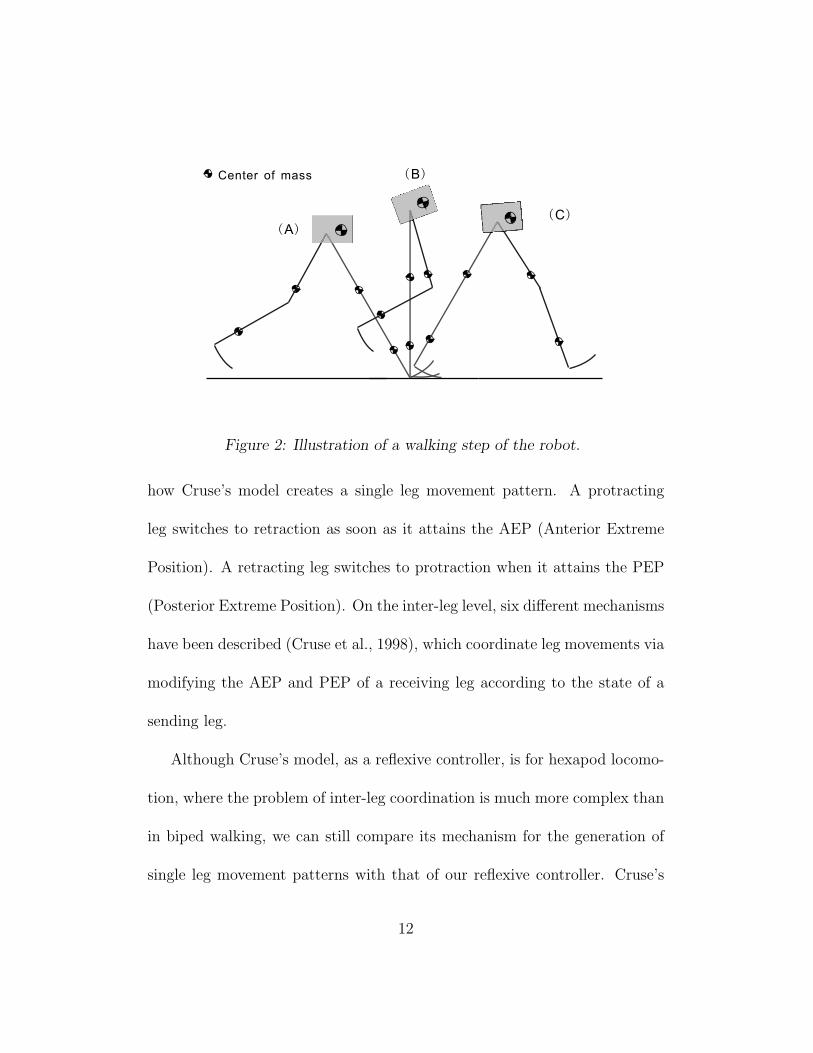
Figure 2: Illustration of a walking step of the robot.
how Cruse’s model creates a single leg movement pattern. A protracting
leg switches to retraction as soon as it attains the AEP (Anterior Extreme
Position). A retracting leg switches to protraction when it attains the PEP
(Posterior Extreme Position). On the inter-leg level, six different mechanisms
have been described (Cruse et al., 1998), which coordinate leg movements via
modifying the AEP and PEP of a receiving leg according to the state of a
sending leg.
Although Cruse’s model, as a reflexive controller, is for hexapod locomo-
tion, where the problem of inter-leg coordination is much more complex than
in biped walking, we can still compare its mechanism for the generation of
single leg movement patterns with that of our reflexive controller. Cruse’s
12

Figure 3: Single leg movement pattern of Cruse’s reflexive controller model
(Cruse et al., 1998).
model depends on PEP, AEP and GC (Ground Contact) signals to generate
the movement pattern of the individual legs. Whereas our reflexive controller
presented here uses only GC and AEA (Anterior Extreme Angle of hip joints)
to trigger switching between stance and swing phases of each leg. Creation
of the single leg movement pattern for our model is illustrated in figure 4.
Figure 4: Illustration of single leg movement pattern generation.
Fig. 4 (A)-(E) represents a series of snapshots of the robot configuration
while it is walking. At the time of figure 4 B, the left foot (black) has just
13
touched the ground. This event triggers four local joint reflexes at the same
time: flexor of left hip, extensor of left knee, extensor of right hip, and flexor
of right knee. At the time of figure 4 E, the right hip joint attains its AEA,
which triggers only the extensor reflex of the right knee. When the right foot
(gray) contacts the ground, a new walking cycle will begin. Note that on the
hip joints and knee joints, extensor means forward movement while flexor
means backward movement.
The reflexive walking controller of our robot follows a hierarchical struc-
ture (see figure 5). The bottom level is the reflex circuit local to the joints,
including motor-neurons and angle sensor neurons involved in joint reflexes.
The top level is a distributed neural network consisting of hip stretch recep-
tors, ground contact sensor neurons, and inter-neurons for reflexes. Neurons
are modelled as non-spiking neurons simulated on a Linux PC, and commu-
nicated to the robot via the DA/AD board. Though somewhat simplified,
they still retain some of the prominent neuronal characteristics.
3.1 Model neuron circuit of the top level
The joint coordination mechanism in the top level is implemented with the
neuron circuit illustrated in figure 5. Each of the ground contact sensor
14

Figure 5: The neuron model of reflexive controller on our robot. Gray circles
= Sensor-neurons or Receptors, Vertical ovals = Inter-neurons, horizontal
ovals = Motor-neurons. Synapses: black circle = excitatory, black triangle
= inhibitory. For meanings of EI, FI, EM, FM, etc. see Table 1.
neurons has excitatory connections to the inter-neurons of the ipsi-lateral
hip flexor and knee extensor as well as to the contra-lateral hip extensor and
15

AL, (AR) Stretch receptor for anterior angle of left (right) hip
GL, (GR) Sensor neuron for ground contact of left (right) foot
EI, (FI) Extensor (Flexor) reflex inter-neuron
EM, (FM) Extensor (Flexor) reflex motor-neuron
ES, (FS) Extensor (Flexor) reflex sensor neuron
Table 1: Meaning of some abbreviations used in this paper.
knee flexor. The stretch receptor of each hip has excitatory connections to its
ipsi-lateral inter-neuron of the knee extensor, and inhibitory connection to
its ipsi-lateral inter-neuron of the knee flexor. Detailed models of the inter-
neuron, stretch receptor, and ground contact sensor neuron are described in
following subsections.
3.1.1 Inter-neuron model
The inter-neuron model is adapted from one used in the neural controller of
a hexapod simulating insect locomotion (Beer and Chiel, 1992). The state
of each model neuron is governed by equations 1,2 (Gallagher et al., 1996):
τidyi
dt= −yi +
∑ωi,juj (1)
uj = (1 + eΘj−yj)−1 (2)
16

Where yi represents the mean membrane potential of the neuron. Equation 2
is a sigmoidal function that can be interpreted as the neuron’s short-term
average firing frequency, Θj is a bias constant that controls the firing thresh-
old. τi is a time constant associated with the passive properties of the cell
membrane (Gallagher et al., 1996), ωi,j represents the connection strength
from the j th neuron to the i th neuron.
3.1.2 Stretch receptors
Stretch receptors play a crucial role in animal locomotion control. When the
limb of an animal reaches an extreme position, its stretch receptor sends a
signal to the controller, resetting the phase of the limbs. There is also evi-
dence that phasic feedback from stretch receptors is essential for maintaining
the frequency and duration of normal locomotive movements in some insects
(Chiel and Beer, 1997).
While other biologically inspired locomotive models and robots use two
stretch receptors on each leg to signal the attaining of the leg’s AEP and PEP
respectively, our robot has only one stretch receptor on each leg to signal the
AEA of its hip joint. Furthermore, the function of the stretch receptor on
our robot is only to trigger the extensor reflex on the knee joint of the same
17
leg, rather than to explicitly (in the case of CPG models) or implicitly (in
the case of reflexive controllers) reset the phase relations between different
legs.
As a hip joint approaches the AEA, the output of the stretch receptors
for the left (AL) and the right hip (AR) are increased as:
ρAL = (1 + eαAL(ΘAL−φ))−1 (3)
ρAL = (1 + eαAR(ΘAR−φ))−1 (4)
Where φ is the real time angular position of the hip joint, ΘAL and ΘAR
are the hip anterior extreme angles whose value are tuned by hand in an
experiment, αAL and αAR are positive constants. This model is inspired
by a sensor neuron model presented in Wadden and Ekeberg (1998) that is
thought capable of emulating the response characteristics of populations of
sensor neurons in animals.
3.1.3 Ground contact sensor neurons
Another kind of sensor neuron incorporated in the top level is the ground
contact sensor neuron, which is active when the foot is in contact with the
ground. Its output, similar to that of the stretch receptors, changes according
18

to:
ρGL = (1 + eαGL(ΘGL−VL+VR))−1 (5)
ρGR = (1 + eαGR(ΘGR−VR+VL))−1 (6)
Where VL and VR are the output voltage signals from piezo sensors of the
left foot and right foot respectively, ΘGL and ΘGR work as thresholds, αGL
and αGR are positive constants.
While AEP and PEP signals account for switching between stance phase
and swing phase in other walking control structures, ground contact signals
play a crucial role in phase transition control of our reflexive controller. This
emphasized role of the ground contact signal also has some biological plau-
sibility. When held in a standing position on a firm flat surface, a newborn
baby will make stepping movements, alternating flexion and extension of
each leg, which looks like ”walking”. This is called “stepping reflex”, elicited
by the foot’s touching of a flat surface. There is considerable evidence that
the stepping reflex, though different from actual walking, eventually develops
into independent walking (Yang et al., 1998).
Concerning its non-linear dynamics, the biped model is hybrid in nature,
containing continuous (in swing phase and stance phase) and discrete (at
the ground contact event) elements. Hurmuzlu applied discrete mapping
19

techniques to study the stability of bipedal locomotion (Hurmuzlu, 1993). It
was found that the timing of ground contact events has a crucial effect on
the stability of biped walking.
Our preference for using a ground contact signal instead of PEP or AEP
signals also has other reasons. In PEP/AEP-models, the movement pattern
of a leg will break down as soon as the AEP or PEP can not be reached,
which may happen as a consequence of an unexpected disturbance from the
environment or due to intrinsic failure. This can be catastrophic for a biped,
though tolerable for a hexapod due to its high degree of redundancy.
3.2 Neural circuit of the bottom level
In animals, a reflex is a local motor response to a local sensation. It is
triggered in response to a suprathreshold stimulus. The quickest reflex in
animals is the ”monosynaptic reflex”, in which the sensor neuron directly
contacts the motor-neuron. The bottom-level reflex system of our robot con-
sists of reflexes local to each joint (see figure 5). The neuron module for
one reflex is composed of one angle sensor neuron and the motor-neuron it
contacts (see figure 5). Each joint is equipped with two reflexes, extensor
reflex and flexor reflex, both are modelled as a monosynaptic reflex, that is,
20

whenever its threshold is exceeded, the angle sensor neuron directly excites
the corresponding motor-neuron. This direct connection between angle sen-
sor neuron and motor-neuron is inspired by a reflex described in cockroach
locomotion (Beer et al., 1997). In addition, the motor-neurons of the local
reflexes also receive an excitatory synapse and an inhibitory synapse from
the inter-neurons of the top level, by which the top level can modulate the
bottom level reflexes.
Each joint has two angle sensor neurons, one for the extensor reflex, and
the other for the flexor reflex (see figure 5). Their models are similar to that
of the stretch receptors described above. The extensor angle sensor neuron
changes its output according to:
ρES = (1 + eαES(φ−ΘES))−1 (7)
where φ is the real time angular position obtained from the potentiometer
of the joint (see figure 1 B). ΘES is the threshold of the extensor reflex (see
figure 1 B) and αES a positive constant.
Likewise, the output of the flexor sensor neuron is modelled as:
ρFS = (1 + eαFS(ΘFS−φ))−1 (8)
where ΘFS and αFS similar as above.
21

It should be particularly noted that the thresholds of the sensor neurons in
the reflex modules do not work as desired positions for joint control, because
our reflexive controller does not involve any exact position control algorithms
that would ensure that the joint positions converge to a desired value. In fact,
as will be shown in the next section, the joints often pass these thresholds in
swing- and stance phase, and begin their passive movement thereafter.
The sensor-neurons involved in the local reflex module of each joint can
only affect the movements of the joint they belong to, having not direct or
indirect connection to other joints. This is different for the phasic feedback
signal, AEA, which works in the top level (i.e., the inter-joint level), sensing
the position of the hip joints and contacting the motor neurons of the knee
joints.
The model of the motor-neuron is the same as that of the inter-neurons
presented in 3.1.1. Note that, on this robot, the output value of the motor-
neurons, after multiplication by a gain coefficient, is sent to the servo ampli-
fier to directly drive the joint motor1. In this way, the neural dynamics are
1While we use motors to drive the robot, animals use muscles for walking.
Muscles have their own special properties that make them particularly suit-
able for walking behaviors, for example, the ”preflex”, which refers to the
22

directly coupled with the motor dynamics, and furthermore, with the biped
walking dynamics. Thus, the robot and its neural controller constitute a
closely coupled neuro-mechanical system.
The voltage of joint motor is determined by
Motor V oltage = MAMP (gEMuEM + gFMuFM) (9)
where MAMP represents the magnitude of the servo amplifier, gEM and gFM
are output gains of the motor-neurons of the extensor- and flexor reflex re-
spectively, uEM and uFM are the outputs of the motor-neurons.
4 Robot walking experiments
The model neuron parameters chosen jointly for all experiments are listed
in Table 2 and 3. Only the thresholds of the sensor neurons and the output
nonlinear, passive visco-elastic properties of the musculoskeletal system of
animals (Brown and Loeb, 1999). Due to the physical nature of the preflex,
the system can respond to disturbances rapidly. In the next stage of our work,
we will build a Hill-type muscle model with RC motors. The motor-neurons
of our reflexive controller at the moment drive the motors directly. In the
next stage, they will drive the muscle model directly, just like in animals.
23

ΘEI ΘFI ΘEM ΘFM αES αFS
Hip Joints 5 5 5 5 4 1
Knee Joints 5 5 5 5 4 4
Table 2: Parameters of neurons for hip- and knee joints. For meaning of the
subscripts, see table 1.
ΘGL (v) ΘGR (v) ΘAL (deg) ΘAR (deg) αGL αGR αAL αAR
2 2 = ΘES = ΘES 4 4 4 4
Table 3: Parameters of stretch receptors and ground contact sensor neurons.
24

Figure 6: Realtime data of one hip joint. (A) Hip joint angle. (B) Motor
voltage measured directly at the motor-neurons of the hip joint. During some
periods (the gray areas), the motor voltage remains zero, and the hip joint
moves passively.
gain of the motor-neurons are changed in different experiments. The time
constants τi of all neurons take the same value of 5ms. The weights of all the
inhibitory connections are set to -10. The weights of all excitatory connec-
tions are 10, except those between inter-neurons and motor-neurons, which
are 0.1.
We encourage readers to watch the video clips of the robot walking experi-
25

Figure 7: Motor voltages of the four joints measured directly at the motor-
neurons, while the robot is walking: (A) left hip; (B) right hip; (C) left knee;
(D) right knee. Note that during one period of every gait cycle (gray area),
all four motor voltages remain zero, and all four joints (i.e., the whole robot)
move passively (see figure 8).
26

ΘES (deg) ΘFS (deg) gEM gFM
Hip Joints 115 70 ±2 ±2
Knee Joints 180 100 ±1.8 ±1.8
Table 4: Specific parameters for walking experiments.
ments:
Walking fast on a flat floor, http://www.cn.stir.ac.uk/˜tgeng/robot/walkingfast.mpg
Walking with a medium speed, http://www.cn.stir.ac.uk/˜tgeng/robot/walkingmedium.mpg
Walking slowly http://www.cn.stir.ac.uk/˜tgeng/robot/walkingslow.mpg
Climbing a shallow slope, http://www.cn.stir.ac.uk/˜tgeng/robot/climbingslope.mpg
These videos can be viewed with Windows Media Player (www.microsoft.com)
or Realplayer (www.real.com).
4.1 Passive movements of the robot
In a walking experiment with specific parameters as given in table 6 the pas-
sive part of the movement of the robot is shown most clearly. (The sign of
gEM and gFM depends on the hardware configurations of the motors on the
left and right leg).
27

Figure 6 shows the motor voltage and the angular movement of one of
its hip joints while the robot is walking. During roughly more than half of
every gait cycle, the hip joint is moving passively.
As shown in figure 7, during some period of every gait cycle (e.g., grey
area in figure 7), the motor voltages of the motor-neurons on all four joints
remain zero, so all joints move passively until the swing leg touches the
ground (see figure 8). During this time, which is roughly one third of a
gait cycle (see figure 7 and figure 8), the movement of the whole robot is
exclusively under the control of ”physical computation” following its passive
dynamics; no feedback based active control acts on it. This demonstrates
very clearly how neurons and mechanical properties work together to generate
the whole gait trajectory. This is also analogous to what happens in animal
locomotion. Muscle control of animals usually exploits the natural dynamics
of their limbs. For instance, during the swing phase of the human walking
gait, the leg muscles first experience a power spike to begin leg swing and
then remain limp throughout the rest of the swing phase, similar to what
is shown in figure 8. Note that, in figure 8 and the corresponding stick
diagrams of walking gait, we omitted the detailed movement of the curved
foot, in order to show clearly the leg-movements. The point on which the
28

stance leg stands is the orthographic projection of the mid-point of the foot
and not its exact ground-contact point.
4.2 Walking at different speeds and a perturbed gait
The walking speed of the robot can be changed easily by adjusting only the
thresholds of the reflex sensor neurons and the output gain of the motor-
neurons (see table 5). Figure 9 A and B show two phase plots of the hip and
knee joint positions, which were recorded while the robot was walking with
different speeds on a flat floor.
Figure 9 C shows a perturbed walking gait. The bulk of the trajectory
represents the normal orbit of the walking gait, while the few outlaying tra-
jectories are caused by external disturbances induced by small obstacles such
as thin books (less than four percent of robot size) obstructing the robot
path. After a disturbance, the trajectory returns to its normal orbit soon,
demonstrating that the walking gaits are stable and to some degree robust
against external disturbances. Here robustness is defined as rapid conver-
gence to a steady state behavior despite unexpected perturbations (Lewis,
2001).
29

ΘES (deg) ΘFS (deg) gEM gFM
Low speed walking Hip Joints 120 70 ±1.4 ±1.3
see Fig. 9 A Knee Joints 180 100 ±1.5 ±1.5
High speed walking Hip Joints 110 85 ±2.5 ±2.5
see Fig. 9 B Knee Joints 180 100 ±1.8 ±1.8
Perturbed walking gait Hip Joints 115 90 ±2.5 ±2.5
see Fig. 9 C Knee Joints 180 100 ±1.5 ±1.5
Table 5: The different values of neuron parameters chosen to generate dif-
ferent speeds (see figure 9).
30

With neuron parameters changed in the cases of fast walking and slow
walking, walking dynamics are implicitly drawn into a different gait cycle
(see figure 9). Figure 9 D shows an experiment in which the neuron param-
eters are changed abruptly online while the robot is walking at a slow speed
(33cm/s, the big orbit). After a short transient stage (the outlaying trajec-
tories), the gait cycle of the robot is automatically transferred into another
stable, high-speed orbit (the small one, 57cm/s). In other words, when the
neuron parameters are changed, physical computation closely coupled with
neural computation can autonomously shift the system into another global
trajectory that is also dynamically stable. This experiment shows that our
biped robot, as a neuro-mechanical system, is stable in a relatively large
domain of its neuron parameters.
With other real-time biped walking controllers based on biologically in-
spired mechanisms (e.g., CPG) or conventional trajectory preplanning and
tracking control, it is still a puzzling problem how to change walking speed on
the fly without undermining dynamical stability at the same time. However,
this experiment shows that the walking speed of our robot can be drastically
changed (nearly doubled) on the fly while the stability is still retained due
to physical computation.
31

4.3 Walking up a shallow slope
Figure 10 is a stick diagram of the robot when it is walking up a shallow slope
of about 4 degrees. Steeper slopes could not be mastered. In figure 10, we
can see that, when the robot is climbing the slope, its step length is becom-
ing smaller, and the movement of its stance leg is becoming slower (its stick
snapshots are becoming denser). Note that these adjustments of its gait take
place autonomously due to the robot’s physical properties (physical computa-
tion), not relying on any pre-planned trajectory or precise control mechanism.
This experiment demonstrates that such a closely coupled neuro-mechanical
system can to some degree autonomously adapt to an unstructured terrain.
5 Stability analysis of the walking gaits
5.1 Dynamic model of the robot
The dynamics of our robot are modelled as shown in figure 11. With the
Lagrange method, we can get the equations that govern the motion of the
robot, which can be written in the form:
D(q)q + C(q, q) +G(q) = τ (10)
32

Where q = [φ, θ1, θ2, ψ]T is a vector describing the configuration of the robot
(for definition of φ, θ1, θ2, ψ, see figure 11). D(q) is the 4× 4 inertia matrix,
C(q, q) is the 4× 1 vector of centripetal and coriolis forces, G(q) is the 4× 1
vector representing gravity forces. τ = [0, τ1, τ2, τ3]T , τ1, τ2, τ3 are the torques
applied on the stance hip (the hip joint of the stance leg in figure 11), the
swing hip, and the swing knee joints, respectively. Details of this equation
can be found in the appendix.
The dynamics of the DC motor (including gears) of each joint can be
described with the following equations (here, the hip of the stance leg is
taken as an example. The models of other joints are likewise):
Ladiadt
+Raia + nk3θ1 = V1 (11)
τ1 + I1θ1 + kf θ1 = nk2ia (12)
Where, V1 is the applied armature voltage of the stance hip motor, which
is obtained from the output of the motor neurons according to equation 9,
ia is the armature current, La the armature inductance, Ra the armature
resistance. k3 is the emf constant. k2 is the motor torque constant. I1
is the combined moment of inertial of the stance-hip motor and gear train
referred to the gear output shaft. kf is the vicious-friction coefficient of the
combination of the motor and the gear. n is the gear ratio.
33

Considering that the electrical time-constant of the motor is much smaller
than the mechanical time-constant of the robot, we neglect the dynamics of
the electrical circuits of the motor, which leads to, diadt
= 0. Thus equation 11
is reduced to,
ia =1
Ra
(V1 − nk3θ1) (13)
Combining equations 10, 12 and 13, we can get the dynamics model of the
robot with the applied motor voltages as its control input.
The heel strike at the end of swing phases and the knee strike at the
end of knee extensor reflex are assumed to be inelastic impacts, which is in
accordance with observations on our real robot and existing passive biped
robots. This assumption implies the conservation of angular momentum of
the robot just before and after the strikes, with which the value of q just after
the strikes can be computed using its value just before the strikes. Because
the transient double support phase is very short in our robot walking (usually
less than 40 ms), it is neglected in our simulation as often done in the analysis
of other passive bipeds (Garcia, 1999).
34

5.2 Stability analysis with Poincare maps
The method of Poincare maps is usually employed for stability analysis of
cyclic movements of non-linear dynamic systems such as passive bipeds (Gar-
cia, 1999). Because our reflexive controller exploits natural dynamics for the
robot’s motion generation, and not trajectory planning or tracking control,
the Poincare map approach can also be applied to the dynamics model of
our robot together with the reflexive network as its controller.
We choose the Poincare section (Garcia, 1999) to be right after the heel
strike of the swing leg. Each cyclic walking gait is a limit cycle in the state
space, corresponding to a fixed point on the Poincare section. Fixed points
can be found by solving the roots of the mapping equation:
P (xn)− xn = 0 (14)
Where xn = [q, q]T = [φ, θ1, θ2, ψ, φ, θ1, θ2, ψ]T
is a state vector on the Poincare
section at the beginning of the nth gait cycle. P (xn) is a map function map-
ping xn to xn+1, which is built by combining the reflexive controller and the
robot dynamics model described above.
Near a fixed point, x∗, the map function P (x∗) can be linearized as (Gar-
35
cia, 1999):
P (x∗ + x) ≈ P (x∗) + Jx (15)
Where J is the 8× 8 Jacobian matrix of partial derivatives of P
J =∂P
∂x(16)
With any fixed point, J can be obtained by numerically evaluating P eight
times in a small neighborhood of the fixed point. According to equation 15,
small perturbations xi to the limit cycle x∗ at the start of ith step will grow
or decay from the ith step to the i + 1th step approximately according to
xi+1 ≈ Jxi. So, if all eigenvalues of J lie within the unit cycle, any small
perturbation will decay to 0 and the perturbed walking gait will return to
its limit cycle, which means the limit cycle is asymptotically stable (Garcia,
1999).
The movements of the knee joints are needed mainly for timely ground
clearance without much influence on the stability of the walking gait. There-
fore, in the simulation analysis and real experiment below we set the knees’
neuron parameters to fixed values (see Table 6) that can ensure fast move-
ments of the knee joints, preventing any possible scuff of the swing leg.
For simplicity, we also fix the threshold of the flexor sensor neurons of the
hips (ΘFS,h) to 85 deg in simulation and real experiments below. This will not
36
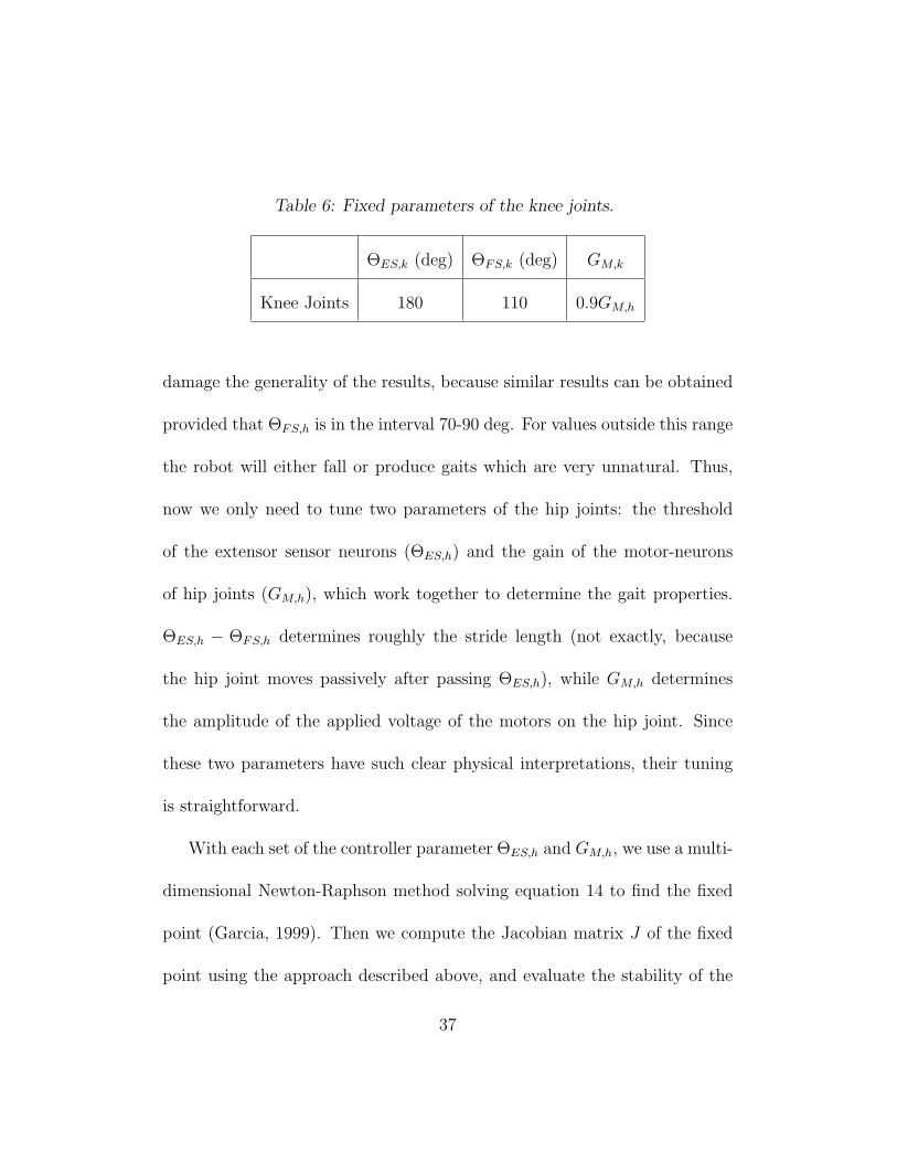
Table 6: Fixed parameters of the knee joints.
ΘES,k (deg) ΘFS,k (deg) GM,k
Knee Joints 180 110 0.9GM,h
damage the generality of the results, because similar results can be obtained
provided that ΘFS,h is in the interval 70-90 deg. For values outside this range
the robot will either fall or produce gaits which are very unnatural. Thus,
now we only need to tune two parameters of the hip joints: the threshold
of the extensor sensor neurons (ΘES,h) and the gain of the motor-neurons
of hip joints (GM,h), which work together to determine the gait properties.
ΘES,h − ΘFS,h determines roughly the stride length (not exactly, because
the hip joint moves passively after passing ΘES,h), while GM,h determines
the amplitude of the applied voltage of the motors on the hip joint. Since
these two parameters have such clear physical interpretations, their tuning
is straightforward.
With each set of the controller parameter ΘES,h and GM,h, we use a multi-
dimensional Newton-Raphson method solving equation 14 to find the fixed
point (Garcia, 1999). Then we compute the Jacobian matrix J of the fixed
point using the approach described above, and evaluate the stability of the
37

fixed point according to its eigenvalues. The result of this Poincare map
analysis is shown in figure 12. We have found that asymptotically stable
fixed points exist in a considerably large range of the controller parameters
ΘES,h and GM,h (see figure 12). For comparison, figure 12 also shows the
stable range of these two parameters obtained in real robot experiments. In
the real robot, because no definite stability criterion, like using eigenvalues,
is applicable, we regard a walking gait as stable if the robot does not fall.
The best way to visualize the properties of a limit cycle is using the phase
plane, which can be easily obtained in the simulations, but is not available
in our real robot due to the lack of absolute position- and speed sensors.
Figure 13 shows two phase plane plots of the absolute angular position of
one hip joint, φ (see figure 11) and its derivative, φ. After being perturbed,
the walking gait returns to its limit cycle quickly in only a few steps, which
is in accordance with the experiment results of the real robot presented in
the last section.
Because some details of the robot dynamics such as uncertainties of the
ground contact, nonlinear frictions in the joints and the inevitable noise
and lag of the sensors are difficult, if not impossible, to model precisely,
the results of simulation and real experiments are not exactly coherent (see
38
figure 12). However, stability analysis and experiments with our real robot
have in general shown that our biped robot under control of the reflexive
network will demonstrate stable walking gaits in a wide range of the critical
controller parameters and that it will return to its normal orbit quickly after
a disturbance.
6 Discussion and comparison with other walk-
ing control mechanisms
6.1 Minimal set of phasic feedbacks
The aim of locomotion control structures (modelled either with CPG or with
reflexive controllers) is to control the phase relations between limbs or joints,
attaining a stable phase locking that leads to a stable gait. Therefore, the
locomotion controller needs phasic feedback from the legs or joints. In the
case of reflexive controllers like Cruse’s model (Cruse et al., 1998), the phasic
feedback signals sent to the controller are AEP and PEP signals, which can
provide sufficient information on phase relations at least between adjacent
legs. It is according to this information that the reflexive controller adjusts
39

the PEP value of the leg, thus effectively changing the period of the leg,
synchronizing it in, or out of phase with its adjacent legs (Klavins et al.,
2002). On the other hand, in the case of a CPG model, which can gen-
erate rhythmic movement patterns even without sensory feedback, it must
nonetheless be entrained to phasic feedback from the legs in order to achieve
realistic locomotion gaits. In some animals, evidence exists that every limb
involved in cyclic locomotion has its own CPG (Delcomyn, 1980), and phasic
feedback from muscles is indispensable to keep its CPGs in phase with the
real time movement of the limbs. Not surprisingly, CPG mechanisms used on
various locomotive robots also require phasic feedback. Lewis et al. (2003)
implemented a CPG oscillator circuit to control a simple biped. AEP and
PEP signals from its hip joints define the feedback to the CPG, resetting its
oscillator circuit. Removal of the AEP or PEP signals caused quick deteri-
oration of this biped’s gait. On another quadruped robot (Fukuoka et al.,
2003), instead of discrete AEP and PEP signals, continuous position signals
of the hip joints provide feedback to the neural oscillators of the CPG. The
neural oscillator parameters were tuned in such a way that the minimum and
maximum of the hip positions would reset the flexor- and extensor oscillator
respectively. Apparently, this scheme functions identically with AEP, PEP
40
feedback.
In summary, because AEP and PEP provide sufficient information about
phase relations between legs, walking control structures usually depend on
them (or their equivalents) as phasic feedback from the legs. However, the
top level of the reflexive controller on our robot requires only AEA signals
as phasic feedback. Furthermore, this AEA signal is only for triggering the
flexor reflex on the knee joint of the robot, rather than triggering stance
phases as in other robots. In this sense, the role (and number) of the phasic
feedback signals is much reduced in our reflexive controller.
In spite of the fact that the AEA signal is by itself not sufficient to control
the phase relations between legs, stable walking gaits have appeared in our
robot walking experiments (see section 4). This is because reflexive controller
and physical computation cooperate to accomplish the task of phasic walking
gait control. This shows that physical computation can help to simplify the
controller structure.
As described above, CPGs have been successfully applied on some real-
time quadruped, hexapod and other multi-legged robots. However, in biped
walking control based on CPG models, most of the current studies are per-
formed with computer simulations. To our knowledge, no one has successfully
41

realized real-time dynamic biped walking using a CPG model as a single con-
troller, because the CPG model itself can not ensure stability of the biped
gait. A considerably well-known biped robot controlled by a CPG chip has
been developed by Lewis et al. (2003). Its walking/running gaits looks very
nice, though on a treadmill instead of on a floor. But this biped robot has
a fatally weak point in that its hips are fixed on a boom (not rotating freely
around the boom axes as in our robot). So it is actually supported by the
boom. The boom is greatly facilitating its control, avoiding the most difficult
problem of dynamic stability control that is specific to biped robots. Thus,
this robot is indeed not a dynamic biped in its real sense. Instead, it is rather
more equivalent to one pair of legs of a multi-legged robot.
Using computer simulations, Taga (1995) found that stable biped gaits
can be generated by combining CPGs and human biomechanics. In animals,
a CPG is a neural structure which is much more complex than the local
reflex in anatomy and function. There is evidence that, in mammal- and
human locomotion, CPGs work on top of reflexes and take their effects via
modulating them. In evolution, simple monosynaptic reflexes must have
appeared much earlier than the much more complex CPG structures. Not
only with simulation analysis, but also with our real system experiments, the
42
current study has shown that local neuronal reflexes connected by a simple
sensor-driven network are sufficient as a controller for dynamic biped walking,
the most difficult form of legged locomotion in view of dynamic stability.
6.2 Physical computation and approximation
In contrast to exact representations and world models, physical computation
often implies approximation. Approximation in control mechanism gives
more room and possibility for physical computation. While conventional
robots rely on precise trajectory planning and tracking control, biologically
inspired robots rarely use preplanned or explicitly computed trajectories. In-
stead, they compute their movements approximately by exploiting physical
properties of their self and the world, thus avoiding the accurate calibration
and modelling required by conventional robotics. But, in order to achieve real
time walking gait in a real world, even these biological inspired robots often
have to depend on some kinds of position- or velocity control on their joints.
For example, on a hexapod, simulating the distributed locomotion control
of insects (Beer et al., 1997), outputs of motor-neurons were integrated to
produce a trajectory of joint positions that was tracked using proportional
feedback position control. On a quadruped, built by Kimura’s group, that
43

implemented CPGs (neural oscillators) and local reflexes, all joints are PD
controlled to move to their desired angles (Fukuoka et al., 2003). Even on
a half passive biped, controlled by a CPG chip, position control worked on
its hip joints, though passive dynamics of its knee joints was exploited for
physical computation (Lewis, 2001).
The principle of approximation embodied in the reflexive controller of
our robot, however, goes even one step further, in the sense that there is no
position or velocity control implemented on our robot. The neural structure
of our reflexive controller does not depend on, or ensure the tracking of,
any desired position. Indeed, it is this approximate nature of our reflexive
controller that allows the physical properties of the robot itself, especially
the passive dynamics of the robot (see figure 8), to contribute implicitly to
generation of overall gait trajectories, and ensures its stability and robustness
to some extent. Just as argued by Raibert and Hodgins 1993, page 353,
”Many researchers in neural motor control think of the nervous system as
a source of commands that are issued to the body as direct orders. We
believe that the mechanical system has a mind of its own, governed by the
physical structure and the laws of physics. Rather than issuing commands,
the nervous system can only make suggestions which are reconciled with the
44

physics of the system and the task.”
7 Conclusions
In this paper, we presented our design and some walking experiments per-
formed by a novel neuro-mechanical structure for reflexive walking control.
We demonstrated with a closely coupled neuro-mechanical system, how phys-
ical computation can be exploited to generate a dynamically stable biped
walking gait. In the experiments of walking at different speeds and climbing
a shallow slope, it was also shown that the coupled dynamics of this neuro-
mechanical system are sufficient to induce an autonomous, albeit limited,
adaptation of the gait.
While the biologically inspired model neurons used in our reflexive con-
troller retain some properties of real neurons, they do not include one of the
most significant features of neurons, namely synaptic plasticity. As has been
observed in human and animal locomotion, while walking gait generation
may be reflexive, stability control of walking behavior has to be predictive.
Although physical computation can assure autonomy and stability to some
extent, in order to get a stable walking gait in a wide parameter range, we
45

have to rely on the plasticity of the neural structure. In the near future,
we will apply proactive learning on this neuro-mechanical system (Porr and
Worgotter, 2003). The basic idea is to use the waveform resulting from the
ground contact sensors to predict and thus avoid possible instabilities of the
next walking step.
Acknowledgement
This work was supported by SHEFC grant INCITE to Prof. F. Worgotter.
We thank Kevin Swingler for correction of the text.
References
Beer, R. and Chiel, H. (1992). A distributed neural network for hexapod
robot locomotion. Neural Computation, 4:356–365.
Beer, R., Quinn, R., Chiel, H., and Ritzmann, R. (1997). Biologically inspired
approaches to robotics. Communications of the ACM, 40(3):30–38.
Boone, G. and Hodgins, J. (1997). Slipping and tripping reflexes for bipedal
robots. Autonomous Robots, 4(3):259–271.
46

Brown, I. and Loeb, G. (1999). Biomechanics and Neural Control of Move-
ment, chapter A reductionist approach to creating and using neuromuscu-
loskeletal models. Springer-Verlag, New York.
Cham, J., Bailey, S., and Cutkosky, M. (2000). Robust dynamic locomotion
through feedforward-preflex interaction. In ASME IMECE Proceedings,
Orlando, Florida.
Chiel, H. and Beer, R. (1997). The brain has a body: adaptive behav-
ior emerges from interactions of nervous system, body, and environment.
Trends in Neuroscience, 20:553–557.
Cruse, H., Kindermann, T., Schumm, M., and et.al. (1998). Walknet - a bio-
logically inspired network to control six-legged walking. Neural Networks,
11(7-8):1435–1447.
Cruse, H. and Saavedra, M. (1996). Curve walking in crayfish. Journal of
Experimental Biology, 199:1477–1482.
Cruse, H. and Warnecke, H. (1992). Coordination of the legs of a slow-walking
cat. Experimental Brain Research, 89:147–156.
47

Delcomyn, F. (1980). Neural basis of rhythmic behavior in animals. Science,
210:492–498.
Ferrell, C. (1995). A comparison of three insect-inspired locomotion con-
trollers. Robotics and Autonomous Systems, 16:135–159.
Fukuoka, Y., Kimura, H., and Cohen, A. (2003). Adaptive dynamic walking
of a quadruped robot on irregular terrain based on biological concepts. Int.
J. of Robotics Research, 22:187–202.
Full, R. J. and Tu, M. S. (1990). Mechanics of six-legged runners. Journal
of Experimental Biology, 148:129–146.
Funabashi, H., Takeda, Y., S., I., and Higuchi, M. (2001). Disturbance com-
pensating control of a biped walking machine based on reflex motions.
JSME International Journal Series C-Mechanical Systems,Machine Ele-
ments and Manufacturing, 44:724–730.
Gallagher, J., Beer, R., Espenschied, K., and Quinn, R. (1996). Applica-
tion of evolved locomotion controllers to a hexapod robot. Robotics and
Autonomous Systems, 19:95–103.
48

Garcia, M. (1999). Stability, scaling, and chaos in passive-dynamic gait mod-
els. PhD thesis, Cornell University.
Hurmuzlu, Y. (1993). Dynamics of bipedal gait; part ii: Stability analysis of
a planar five-link biped. ASME Journal of Applied Mechanics, 60(2):337–
343.
Iida, F. and Pfeifer, R. (2004). Self-stabilization and behavioral diversity
of embodied adaptive locomotion. Lecture notes in artificial intelligence,
3139:119–129.
Klavins, E., Komsuoglu, H., Full, R., and Koditschek, D. (2002). Neurotech-
nology for Biomimetic Robots, chapter The Role of Reflexes Versus Central
Pattern Generators in Dynamical Legged Locomotion. MIT Press.
Lewis, M. (2001). Certain principles of biomorphic robots. Autonomous
Robots, 11:221–226.
Lewis, M., Etienne-Cummings, R., Hartmann, M., Xu, Z., and Cohen, A.
(2003). An in silico central pattern generator: Silicon oscillator, coupling,
entrainment, and physical computation. Biological Cybernetics, 88:137–
151.
49
Porr, B. and Worgotter, F. (2003). Isotropic sequence order learning. Neural
Comp., 15:831–864.
Porr, B. and Worgotter, F. (2005). Inside embodiment what means embod-
iment for radical constructivists? Kybernetes, 34:105–117.
Pratt, J. (2000). Exploiting Inherent Robustness and Natural Dynamics in the
Control of Bipedal Walking Robots. PhD thesis, Massachusetts Institute of
Technology.
Raibert, H. and Hodgins, J. (1993). Biological Neural Networks in Inverte-
brate Neuroethology and Robotics, chapter Legged robots, pages 319–354.
Academic Press, Boston.
Reeve, R. (1999). Generating walking behaviors in legged robots. PhD thesis,
University of Edinburgh.
Taga, G. (1995). A model of the neuro-musculo-skeletal systems for human
locomotion. Biological Cybernetics, 73:97–111.
Van der Linde, R. Q. V. (1998). Active leg compliance for passive walk-
ing. In Proceedings of IEEE International Conference on Robotics and
Automation, Orlando, Florida.
50
Wadden, T. and Ekeberg, O. (1998). A neuro-mechanical model of legged
locomotion: Single leg control. Biological Cybernetics, 79:161–173.
Yang, J., Stephens, M., and Vishram, R. (1998). Infant stepping: A method
to study the sensory control of human walking. J. Physiol (London),
507:927–937.
Ziemke, T. (2001). Are robots embodied? In First international workshop on
epigenetic robotics Modeling Cognitive Development in Robotic Systems.
Appendix
In the following we list the terms of the equation used in the simulation to
build the Poincare map function. For definitions of l1, l2, l3, l4, l5, φ, θ1, θ2, ψ,
see figure 11. r is the radius of the curved foot. mt is the mass of the trunk,
mh the mass of the thigh, mk the mass of the shank with foot. g is the
gravity.
D11 = −4mk cos (φ) r2 − 2mkl4l2 + 2mkrl4 + 2mk
(l1
2 + l22)
+2mtl1l2 − 2l1r − 2mtrl2
+4mkr cos (φ) l2 − 2mkr cos (φ) l4 + 2mkl42 + 2mtr cos (φ) l2
+2mtl2l5 cos (θ1)− 2mtrl5 cos (θ1)
51
+2mtr cos (φ) l1 + 2mtrl5 cos (θ1 − φ) + 2mtl1l5 cos (θ1)
−2mt cos (φ) r2 +mtl52
−4mh cos (φ) r2 − 2mhl1l3 − 2mhl2l3
+2mhrl3 + 2mkl1l2 − 2mkl1r − 4mkrl2 + 4mkr2
+2mkl22 + 4mhl1l2 − 4mhl1r − 4mhrl2
+2mhl12 + 4mhr
2 + 2mhl22
−2mhrl3 cos (−θ2 + φ)
−2mhl1l3 cos (−θ1 + θ2)− 2mhl2l3 cos (−θ1 + θ2)
+2mhrl3 cos (−θ1 + θ2)− 2mkrl4 cos (−θ2 + ψ)
+2mkrl4 cos (−θ1 + θ2 + ψ + φ)
−2mkrl1 cos (−θ1 + θ2 + φ)
−2mkl1l4 cos (ψ) + 2mkl4l2 cos (−θ1 + θ2 + ψ)
+2mkl1l4 cos (−θ1 + θ2 + ψ)
+2mkrl1 cos (−θ1 + θ2) + 4mhr cos (φ) l2
−2mhr cos (φ) l3 + 4mhr cos (φ) l1
−2mkl12 cos (−θ1 + θ2)
+2mhl32 +mtl1
2 + 2mtr2
D12 = −mtrl5 cos (θ1 − φ) +mtrl5 cos (θ1)
52
−mt(l1 + l2)l5 cos (θ1)
−mtmhrl3 cos (−θ1 + θ2 + φ)
−mhrl3 cos (−θ1 + θ2) +mhl2l3 cos (−θ1 + θ2)
+mhl1l3 cos (−θ1 + θ2)−mhl32
+mkrl1 cos (−θ1 + θ2 + φ)−mkrl4 cos (−θ1 + θ2 + ψ + φ)
+mkl2l1 cos (−θ1 + θ2)−mkrl1 cos (−θ1 + θ2)
+2mkl1l4 cos (ψ)
+mkl12 cos (−θ1 + θ2)
+mkl1l4 cos (−θ1 + θ2 + ψ)
−mkl4l2 cos (−θ1 + θ2 + ψ)
+mkrl4 cos (−θ1 + θ2 + ψ)
−mkl12 −mkl4
2
D13 = −mhrl3 cos (−θ1 + θ2 + φ)
+mhrl3 cos (−θ1 + θ2)−mhl2l3 cos (−θ1 + θ2)
−mhl1l3 cos (−θ1 + θ2) +mhl32 +mkl1
2 −mkrl1 cos (−θ1 + θ2)
+mkrl4 cos (−θ1 + θ2) +mkl2l1 cos (−θ1 + θ2)
+mkrl1 cos (−θ1 + θ2)
−2mkl1l4 cos (ψ)−mkl12 cos (−θ1 + θ2)
53
+mkl1l4 cos (−θ1 + θ2 + ψ)
+mkl4l2 cos (−θ1 + θ2 + ψ)
−mkrl4 cos (−θ1 + θ2 + ψ) +mkl12 +mkl4
2
D14 = mkrl4 cos (−θ1 + θ2 + ψ + φ)
−mkrl4 cos (−θ1 + θ2 + ψ)
+mkl4 (l1 + l2) cos (−θ1 + θ2 + ψ)
−mkl1l4 cos (ψ) +mkl42
D21 = D12
D22 = mtl52 +mhl3
2 +mkl12 − 2mkl1l4 cos (ψ) +mkl4
2
D23 = −mhl32 −mkl1
2 + 2mkl1l4 cos (ψ)−mkl42
D24 = mkl1l4 cos (ψ)−mkl42
D31 = D13
54

D32 = D23
D33 = mhl32 +mkl1
2 − 2l1l4 cos (ψ) +mkl42
D34 = −mkl1l4 cos (ψ) +mkl42
D41 = D14
D42 = D24
D43 = D34
D44 = mkl42
C1 = 2mk sin (φ) φ2r2 − 4mk sin (φ) φ2l2r
−2mt sin (φ) φ2(l1 + l2)r
+2mtl5 sin (θ1 − φ) φ2r
−2mtl5 cos (θ1 − φ) θ1 sin (φ) φl1
+mtl5 sin (θ1 − φ) θ12r
55

+2mt sin (φ) φ2r2 + 4mh sin (φ) φ2r2
−3mtl5 sin (θ1 − φ) θ1φr
+2mtl5 sin (θ1 − φ) θ1φ cos (φ) r
+2mhl3 sin (φ) φ2r
+mhl3 sin (−θ1 + θ2 + φ) θ12r
+2mhl3 cos (−θ1 + θ2 + φ) θ2 sin (φ) φr
+2mhl3 cos (−θ1 + θ2 + φ) θ1θ2 sin (φ) l2
+2mhl3 cos (−θ1 + θ2 + φ) θ1θ2 sin (φ) l1
−mhl3 cos (−θ1 + θ2 + φ) θ12sin (φ) l2
+3mhl3 sin (−θ1 + θ2 + φ) θ2φr
−mkl1 sin (−θ1 + θ2 + φ) θ12cos (φ) r
+2mkl1 sin (−θ1 + θ2 + φ) θ1θ2 cos (φ) r
−2mkl12 sin (−θ1 + θ2 + φ) θ1θ2 cos (φ)
−2mkl1 sin (−θ1 + θ2 + φ) θ1θ2 cos (φ) l2
−2mkl1 sin (−θ1 + θ2 + φ) θ2φ cos (φ) r
+2mkl4 cos (−θ1 + θ2 + ψ + φ) θ2ψ sin (φ) l2
−2mkl1 sin (−θ1 + θ2 + φ) θ1φ cos (φ) l2
−2mkl12 sin (−θ1 + θ2 + φ) θ1φ cos (φ)
+mkl12 sin (−θ1 + θ2 + φ) θ1
2cos (φ)
56

+mkl4 cos (−θ1 + θ2 + ψ + φ) ψ2 sin (φ) l1
−2mkl4 cos (−θ1 + θ2 + ψ + φ) θ2ψ sin (φ) r
+mkl4 cos (−θ1 + θ2 + ψ + φ) θ22sin (φ) l1
+2mkl4 cos (−θ1 + θ2 + ψ + φ) θ2ψ sin (φ) l1
+mkl4 cos (−θ1 + θ2 + ψ + φ) θ22sin (φ) l2
−mkl4 cos (−θ1 + θ2 + ψ + φ) ψ2l1 sin (−θ1 + θ2 + φ)
−mkl4 cos (−θ1 + θ2 + ψ + φ) θ22sin (φ) r
−2mkl4 cos (−θ1 + θ2 + ψ + φ) θ1θ2 sin (φ) l1
+2l4 cos (−θ1 + θ2 + ψ + φ) θ1θ2 sin (φ) r
+2mkl4 cos (−θ1 + θ2 + ψ + φ) θ1ψ sin (φ) r
+2mkl12 cos (−θ1 + θ2 + φ) θ1θ2 sin (φ)
−mkl1 cos (−θ1 + θ2 + φ) θ12sin (φ) l2
−mkl12 cos (−θ1 + θ2 + φ) θ1
2sin (φ)
+mkl1 cos (−θ1 + θ2 + φ) θ12sin (φ) r
+mkl4 cos (−θ1 + θ2 + ψ + φ) θ12sin (φ) l2
+2mkl4 cos (−θ1 + θ2 + ψ + φ) ψ sin (φ) φl2
−2mkl4 cos (−θ1 + θ2 + ψ + φ) θ1ψ sin (φ) l1
−2l1 cos (−θ1 + θ2 + φ) θ1θ2 sin (φ) r
−2mkl4 cos (−θ1 + θ2 + ψ + φ) ψl1 sin (−θ1 + θ2 + φ) θ2
57
−2mkl4 cos (−θ2 + ψ + φ) ψl1 sin (−θ1 + θ2 + φ) φ
−2mkl4 cos (−θ1 + θ2 + ψ + φ) ψ sin (φ) φr
−mkl4 cos (−θ1 + θ2 + ψ + φ) θ12sin (φ) r
−2mkl4 cos (−θ1 + θ2 + ψ + φ) θ1ψ sin (φ) l2
−2mkl4 cos (−θ1 + θ2 + ψ + φ) θ1θ2 sin (φ) l2
−mkl12 cos (−θ1 + θ2 + φ) θ2
2sin (φ)
+mkl1 cos (−θ1 + θ2 + φ) θ22sin (φ) r
−mhl3 sin (−θ1 + θ2 + φ) θ22cos (φ) r
−2mhl3 sin (−θ1 + θ2 + φ) θ2φ cos (φ) r
−mkl1 cos (−θ1 + θ2 + φ) θ22sin (φ) l2
+mhl3 sin (−θ1 + θ2 + φ) θ22cos (φ) l2
+mhl3 sin (−θ1 + θ2 + φ) θ22cos (φ) r
+mhl3 sin (−θ1 + θ2 + φ) θ1φr
+2mhl3 sin (−θ1 + θ2 + φ) θ2φ cos (φ) l2
+mhl3 sin (−θ1 + θ2 + φ) θ22r
−2mkl1 cos (−θ1 + θ2 + φ) θ1 sin (φ) φr
+2mkl1 cos (−θ1 + θ2 + φ) θ1 sin (φ) φl2
+2mkl1 cos (−θ1 + θ2 + φ) θ1θ2 sin (φ) l2
−mhl3 cos (−θ1 + θ2 + φ) θ22sin (φ) l2
58

−mhl3 cos (−θ1 + θ2 + φ) θ22sin (φ) l1
−mhl3 sin (−θ1 + θ2 + φ) θ12cos (φ) r
−2mhl3 cos (−θ1 + θ2 + φ) θ1θ2 sin (φ) r
+mhl3 cos (−θ1 + θ2 + φ) θ22sin (φ) r
−2mhl3 sin (−θ1 + θ2 + φ) θ1φ cos (φ) l1
−mhl3 cos (−θ1 + θ2 + φ) θ12sin (φ) l1
+2mhl3 sin (−θ1 + θ2 + φ) θ1θ2 cos (φ) r
+2mhl3 sin (−θ1 + θ2 + φ) θ1φ cos (φ) r
−2mhl3 sin (−θ2 + φ) θ1φ cos (φ) l2
+mhl3 sin (−θ1 + θ2 + φ) θ12cos (φ) l2
+mhl3 sin (−θ1 + θ2 + φ) θ12cos (φ) l1
−2mhl3 sin (−θ1 + θ2 + φ) θ1θ2 cos (φ) l2
+2mhl3 cos (−θ1 + θ2 + φ) θ1 sin (φ) φl2
+2mhl3 cos (−θ1 + θ2 + φ) θ1 sin (φ) φl1
+2mhl3 sin (−θ1 + θ2 + φ) θ2φ cos (φ) l1
−2mhl3 cos (−θ1 + θ2 + φ) θ2 sin (φ) φl1
−4mh sin (φ) φ2l2r
−4mh sin (φ) φ2l1r
+2mhl3 sin (−θ1 + θ2 + φ) φ2r
59

−2mtl5 cos (θ1 − φ) θ1 sin (φ) φl2
+mtl5 cos (θ1 − φ) θ12sin (φ) l2
+mtl5 cos (θ1 − φ) θ12sin (φ) l1
−mtl5 cos (θ1 − φ) θ12sin (φ) r
+mhl3 cos (−θ1 + θ2 + φ) θ12sin (φ) r
−mtl5 sin (θ1 − φ) θ12cos (φ) r
−2mtl5 sin (θ1 − φ) θ1φ cos (φ) l2
+2mtl5 cos (θ1 − φ) θ1 sin (φ) φr
+mtl5 sin (θ1 − φ) θ12cos (φ) l2
+mtl5 sin (θ1 − φ) θ12cos (φ) l1
−2mtl5 sin (θ1 − φ) θ1φ cos (φ) l1
+2mkl4 sin (−θ1 + θ2 + ψ + φ) θ1θ2r
−3mkl4 sin (−θ1 + θ2 + ψ + φ) ψφr
−mkl4 sin (−θ1 + θ2 + ψ + φ) ψ2 cos (φ) l2
+2mkl4 sin (−θ1 + θ2 + ψ + φ) θ1ψr
−3mkl4 sin (−θ1 + θ2 + ψ + φ) θ2φr
+3mkl4 sin (−θ1 + θ2 + ψ + φ) θ1φr
−2mkl4 sin (−θ1 + θ2 + ψ + φ) ψφ cos (φ) l2
−mkl4 sin (−θ1 + θ2 + ψ + φ) θ22r
60

−mkl4 sin (−θ1 + θ2 + ψ + φ) θ12r
−2mkl4 cos (−θ1 + θ2 + ψ + φ) θ1 sin (φ) φl2
−2mk sin (φ) φ2l1r
+mkl1 sin (−θ1 + θ2 + φ) θ12r
+2mkl1 sin (−θ1 + θ2 + φ) φ2r
+3mkl1 sin (−θ1 + θ2 + φ) θ2φr
−2mkl1 sin (−θ1 + θ2 + φ) θ1θ2r
−2mkl4 sin (−θ1 + θ2 + ψ + φ) θ2φ cos (φ) l2
−2mkl4 sin (−θ1 + θ2 + ψ + φ) θ2φ cos (φ) l1
+2mkl4 sin (−θ1 + θ2 + ψ + φ) ψφ cos (φ) r
+2mkl4 sin (−θ1 + θ2 + ψ + φ) θ2φ cos (φ) r
+2mkl4 sin (−θ1 + θ2 + ψ + φ) θ1ψ cos (φ) l1
+2mkl4 sin (−θ1 + θ2 + ψ + φ) θ2ψl1 cos (−θ1 + θ2 + φ)
−mkl4 sin (−θ1 + θ2 + ψ + φ) θ12cos (φ) l2
−3mkl1 sin (−θ1 + θ2 + φ) θ1φr
+mkl1 sin (−θ1 + θ2 + φ) θ22r
−mkl4 sin (−θ1 + θ2 + ψ + φ) θ12cos (φ) l1
−2mkl4 sin (−θ1 + θ2 + ψ + φ) θ2ψ cos (φ) l2
−2mkl4 sin (−θ1 + θ2 + ψ + φ) θ2ψ cos (φ) l1
61

+mkl4 sin (−θ1 + θ2 + ψ + φ) θ22cos (φ) r
+2mkl4 sin (−θ1 + θ2 + ψ + φ) θ2ψ cos (φ) r
−mkl4 sin (−θ1 + θ2 + ψ + φ) θ22cos (φ) l2
+4mk sin (φ) φ2r2
+2mkl4 sin (−θ1 + θ2 + ψ + φ) θ1φ cos (φ) l1
−mkl4 sin (−θ1 + θ2 + ψ + φ) θ22cos (φ) l1
+2mkl1 sin (−θ1 + θ2 + φ) θ2φ cos (φ) l2
+2mkl12 sin (−θ1 + θ2 + φ) θ2φ cos (φ)
−2mkl4 sin (−θ1 + θ2 + ψ + φ) φ2r
+2mkl4 sin (−θ1 + θ2 + ψ + φ) θ1θ2 cos (φ) l2
+2mkl4 sin (−θ1 + θ2 + ψ + φ) θ1ψ cos (φ) l2
−2mkl4 sin (−θ1 + θ2 + ψ + φ) θ1θ2 cos (φ) r
−2mkl4 sin (−θ1 + θ2 + ψ + φ) θ1ψl1 cos (−θ1 + θ2 + φ)
−2mkl4 sin (−θ1 + θ2 + ψ + φ) θ1φ cos (φ) r
+2mkl4 sin (−θ1 + θ2 + ψ + φ) θ1φ cos (φ) l2
+mkl4 sin (−θ1 + θ2 + ψ + φ) θ12cos (φ) r
+mkl1 sin (−θ1 + θ2 + φ) θ22cos (φ) l2
+2mkl4 sin (−θ1 + θ2 + ψ + φ) θ1θ2 cos (φ) l1
−2mkl4 sin (−θ1 + θ2 + ψ + φ) θ1ψ cos (φ) r
62

+mkl12 sin (−θ1 + θ2 + φ) θ2
2cos (φ)
−mkl4 sin (−θ1 + θ2 + ψ + φ) ψ2r
−mkl4 cos (−θ1 + θ2 + ψ + φ) ψ2 sin (φ) r
+mkl4 cos (−θ1 + θ2 + ψ + φ) ψ2 sin (φ) l2
+2mkl1 sin (−θ1 + θ2 + φ) θ1φ cos (φ) r
+mkl1 sin (−θ1 + θ2 + φ) θ12cos (φ) l2
−2mkl4 cos (−θ1 + θ2 + ψ + φ) θ1 sin (φ) φl1
+2mkl4 cos (−θ1 + θ2 + ψ + φ) ψ sin (φ) φl1
+2mkl4 cos (−θ1 + θ2 + ψ + φ) ψl1 sin (−θ1 + θ2 + φ) θ1
−2mhl3 cos (−θ1 + θ2 + φ) θ2 sin (φ) φl2
−2mhl3 cos (−θ1 + θ2 + φ) θ1 sin sin (φ) φr
+2mkl4 cos (−θ1 + θ2 + ψ + φ) θ1 sin (φ) φr
+2mkl4 cos (−θ1 + θ2 + ψ + φ) θ2 sin (φ) φl2
+2mkl4 cos (−θ1 + θ2 + ψ + φ) θ2 sin (φ) φl1
−2mkl4 cos (−θ1 + θ2 + ψ + φ) θ2 sin (φ) φr
+2mkl12 cos (−θ1 + θ2 + φ) θ1 sin (φ) φ
+mkl4 sin (−θ1 + θ2 + ψ + φ) ψ2 cos (φ) r
−2mkl4 sin (−θ1 + θ2 + ψ + φ) ψφ cos (φ) l1
+2mkl1 cos (−θ1 + θ2 + φ) θ2 sin (φ) φr
63

−2mkl12 cos (−θ1 + θ2 + φ) θ2 sin (φ) φ
−2mkl4 sin (−θ1 + θ2 + ψ + φ) θ2ψr
+2mkl4 sin (−θ1 + θ2 + ψ + φ) ψφl1 cos (−θ1 + θ2 + φ)
C2 = −mtl5 sin (θ1 − φ) φ2r
+mtl5 cos (θ1 − φ) θ1 sin (φ) φl1
+mtl5 sin (θ1 − φ) θ1φr
−mtl5 sin (θ1 − φ) θ1φ cos (φ) r
+mkl1 sin (−θ1 + θ2 + φ) θ2φ cos (φ) r
+mkl1 sin (−θ1 + θ2 + φ) θ1φ cos (φ) l2
+mkl12 sin (−θ1 + θ2 + φ) θ1φ cos (φ)
+mkl4 cos (−θ1 + θ2 + ψ + φ) ψ2l1 sin (−θ1 + θ2 + φ)
−mkl4 cos (−θ1 + θ2 + ψ + φ) ψ sin (φ) φl2
+2mkl4 cos (−θ1 + θ2 + ψ + φ) ψl1 sin (−θ1 + θ2 + φ) θ2
+2mkl4 cos (−θ1 + θ2 + ψ + φ) ψl1 sin (−θ1 + θ2 + φ) φ
+mkl4 cos (−θ1 + θ2 + ψ + φ) ψ sin (φ) φr
+mhl3 sin (−θ1 + θ2 + φ) θ2φ cos (φ) r
−mhl3 sin (−θ1 + θ2 + φ) θ2φ cos (φ) l2
−mkl1 cos (−θ1 + θ2 + φ) θ1 sin (φ) φl2
64

+mhl3 sin (−θ1 + θ2 + φ) θ1φ cos (φ) l1
−mhl3 sin (−θ1 + θ2 + φ) θ1φ cos (φ) r
+mhl3 sin (−θ1 + θ2 + φ) θ1φ cos (φ) l2
−mhl3 cos (−θ1 + θ2 + φ) θ1 sin (φ) φl2
−mhl3 cos (−θ1 + θ2 + φ) θ1 sin (φ) φl1
−mhl3 sin (−θ1 + θ2 + φ) θ2φ cos (φ) l1
−mhl3 sin (−θ1 + θ2 + φ) φ2r
+mtl5 cos (θ1 − φ) θ1 sin (φ) φl2
+mtl5 sin (θ1 − φ) θ1φ cos (φ) l2
−mtl5 cos (θ1 − φ) θ1 sin (φ) φr
+mtl5 sin (θ1 − φ) θ1φ cos (φ) l1
+mkl4 sin (−θ1 + θ2 + ψ + φ) ψφr
+mkl4 sin (−θ1 + θ2 + ψ + φ) θ2φr
−mkl4 sin (−θ1 + θ2 + ψ + φ) θ1φr
+mkl4 sin (−θ1 + θ2 + ψ + φ) ψφ cos (φ) l2
+mkl4 cos (−θ1 + θ2 + ψ + φ) θ1 sin (φ) φl2
−mkl1 sin (−θ1 + θ2 + φ) φ2r
−mkl1 sin (−θ1 + θ2 + φ) θ2φr
−mkl4 sin (−θ1 + θ2 + ψ + φ) ψ2l1 cos (−θ1 + θ2 + φ)
65
−mkl4 sin (−θ1 + θ2 + ψ + φ) ψφ cos (φ) r
−mkl4 sin (−θ1 + θ2 + ψ + φ) θ2φ cos (φ) r
−2mkl4 sin (−θ1 + θ2 + ψ + φ) θ2ψl1 cos (−θ1 + θ2 + φ)
+mkl1 sin (−θ1 + θ2 + φ) θ1φr
−mkl4 sin (−θ1 + θ2 + ψ + φ) θ1φ cos (φ) l1
−mkl1 sin (−θ1 + θ2 + φ) θ2φ cos (φ) l2
−mkl12 sin (−θ1 + θ2 + φ) θ2φ cos (φ)
+mkl4 sin (−θ1 + θ2 + ψ + φ) φ2r
+2mkl4 sin (−θ1 + θ2 + ψ + φ) θ1ψl1 cos (−θ1 + θ2 + φ)
+mkl4 sin (−θ1 + θ2 + ψ + φ) φ cos (φ) r
−mkl4 sin (−θ1 + θ2 + ψ + φ) θ1φ cos (φ) l2
−mkl1 sin (−θ1 + θ2 + φ) θ1φ cos (φ) r
+mkl1 cos (−θ1 + θ2 + φ) θ2 sin (φ) φl2
+mkl4 cos (−θ2 + ψ + φ) θ1 sin (φ) φl1
−mkl4 cos (−θ1 + θ2 + ψ + φ) sin (φ) φl1
−2mkl4 cos (−θ1 + θ2 + ψ + φ) ψl1 sin (−θ1 + θ2 + φ) θ1
+mhl3 cos (−θ1 + θ2 + φ) θ2 sin (φ) φl2
+mhl3 cos (−θ1 + θ2 + φ) θ1 sin (φ) φr
−mkl4 cos (−θ1 + θ2 + ψ + φ) θ1 sin (φ) φr
66

−mkl4 cos (−θ1 + θ2 + ψ + φφ) φl1
+mkl4 cos (−θ1 + θ2 + ψ + φ) θ2 sin (φ) φr
−mkl12 cos (−θ1 + θ2 + φ) θ1 sin (φ) φ
+mkl4 sin (−θ1 + θ2 + ψ + φ) ψφ cos (φ) l1
−mkl1 cos (−θ1 + θ2 + φ) θ2 sin (φ) φr
+mkl12 cos (−θ1 + θ2 + φ) θ2 sin (φ) φ
−2mkl4 sin (−θ1 + θ2 + ψ + φ) ψφl1 cos (−θ1 + θ2 + φ)
C3 = mhl3 cos (−θ1 + θ2 + φ) θ2 sin (φ) φr
+mhl3 sin (−θ1 + θ2 + φ) θ2φr
−mkl1 sin (−θ1 + θ2 + φ) φ cos (φ) r
−mkl1 sin (−θ1 + θ2 + φ) θ1φ cos (φ) l2
−mkl4 cos (−θ1 + θ2 + ψ + φ) ψ2l1 sin (−θ1 + θ2 + φ)
−mkl4 cos (−θ1 + θ2 + ψ + φ) ψ sin (φ) φr
+mhl3 sin (−θ1 + θ2 + φ) θ2φ cos (φ) l2
−mkl1 cos (−θ1 + θ2 + φ) θ1 sin (φ) φr
+mkl1 cos (−θ1 + θ2 + φ) θ1 sin (φ) φl2
−mhl3 sin (−θ1 + θ2 + φ) θ1φ cos (φ) l1
+mhl3 sin (−θ1 + θ2 + φ) θ1φ cos (φ) r
67

−mhl3 sin (−θ1 + θ2 + φ) θ1φ cos (φ) l2
+mhl3 cos (−θ1 + θ2 + φ) θ1 sin (φ) φl2
+mhl3 cos (−θ1 + θ2 + φ) θ1 sin (φ) φl1
−mhl3 cos (−θ1 + θ2 + φ) θ2 sin (φ) φl1
+mhl3 sin (−θ1 + θ2 + φ) φ2r
−mkl4 sin (−θ1 + θ2 + ψ + φ) ψφr
−mkl4 sin (−θ1 + θ2 + ψ + φ) θ2φr
+mkl4 sin (−θ1 + θ2 + ψ + φ) θ1φr
−mkl4 sin (−θ2 + ψ + φ) ψφ cos (φ) l2
−mkl4 cos (−θ1 + θ2 + ψ + φ) θ1 sin (φ) φl2
+mkl1 sin (−θ1 + θ2 + φ) φ2r
+mkl1 sin (−θ1 + θ2 + φ) θ2φr
−mkl4 sin (−θ1 + θ2 + ψ + φ) θ2φ cos (φ) l2
+mkl4 sin (−θ1 + θ2 + ψ + φ) θ2φ cos (φ) l1
+mkl4 sin (−θ1 + θ2 + ψ + φ) ψφ cos (φ) r
+mkl4 sin (−θ1 + θ2 + ψ + φ) θ2φ cos (φ) r
+2mkl4 sin (−θ1 + θ2 + ψ + φ) θ2ψl1 cos (−θ1 + θ2 + φ)
−mkl1 sin (−θ1 + θ2 + φ) θ1φr
+mkl4 sin (−θ1 + θ2 + ψ + φ) θ1φ cos (φ) l1
68
+mkl1 sin (−θ1 + θ2 + φ) θ2φ cos (φ) l2
+mkl12 sin (−θ1 + θ2 + φ) θ2φ cos (φ)
−mkl4 sin (−θ1 + θ2 + ψ + φ) φ2r
−2mkl4 sin (−θ1 + θ2 + ψ + φ) θ1ψl1 cos (−θ1 + θ2 + φ)
−mkl4 sin (−θ1 + θ2 + ψ + φ) φ cos (φ) r
+mkl4 sin (−θ1 + θ2 + ψ + φ) θ1φ cos (φ) l2
+mkl1 sin (−θ1 + θ2 + φ) θ1φ cos (φ) r
−mkl1 cos (−θ1 + θ2 + φ) θ2 sin (φ) φl2
−mkl4 cos (−θ1 + θ2 + ψ + φ) θ1 sin (φ) φl1
+mkl4 cos (−θ1 + θ2 + ψ + φ) ψ sin (φ) φl1
+2mkl4 cos (−θ1 + θ2 + ψ + φ) ψl1 sin (−θ1 + θ2 + φ) θ1
−mhl3 cos (−θ1 + θ2 + φ) θ2 sin (φ) φl2
−mhl3 cos (−θ1 + θ2 + φ) θ1 sin (φ) φr
+mkl4 cos (−θ1 + θ2 + ψ + φ) θ1 sin (φ) φr
+mkl4 cos (−θ1 + θ2 + ψ + φ) θ2 sin (φ) φl2
+mkl4 cos (−θ1 + θ2 + ψ + φ) θ2 sin (φ) φl1
−mkl4 cos (−θ1 + θ2 + ψ + φ) θ2 sin (φ) φr
+mkl12 cos (−θ1 + θ2 + φ) θ1 sin (φ) φ
−mkl4 sin (−θ1 + θ2 + ψ + φ) ψφ cos (φ) l1
69

+mkl1 cos (−θ1 + θ2 + φ) θ2 sin (φ) φr
−mkl12 cos (−θ1 + θ2 + φ) θ2 sin (φ) φ
+2mkl4 sin (−θ1 + θ2 + ψ + φ) ψφl1 cos (−θ1 + θ2 + φ)
C4 = −mkl4 sin (−θ1 + θ2 + ψ + φ) rφ2
+mkl4 cos (−θ1 + θ2 + ψ + φ) sin (φ) φl1ψ
+mkl4 cos (−θ1 + θ2 + ψ + φ) sin (φ) φl2ψ
−mkl4 cos (−θ1 + θ2 + ψ + φ) sin (φ) φrψ
−mkl4 cos (−θ1 + θ2 + ψ + φ) l1 sin (−θ1 + θ2 + φ) φψ
+mkl4 cos (−θ1 + θ2 + ψ + φ) sin (φ) φrθ1
+mkl4 sin (−θ1 + θ2 + ψ + φ) cos (φ) φrψ
+mkl4 cos (−θ1 + θ2 + ψ + φ) l1 sin (−θ1 + θ2 + φ) θ1ψ
−mkl4 sin (−θ1 + θ2 + ψ + φ) cos (φ) φl1ψ
+mkl4 sin (−θ1 + θ2 + ψ + φ) l1 cos (−θ1 + θ2 + φ) φψ
−mkl4 cos (−θ1 + θ2 + ψ + φ) sin (φ) φl2θ1
−mkl4 cos (−θ1 + θ2 + ψ + φ) sin (φ) φrθ2
+mkl4 cos (−θ1 + θ2 + ψ + φ) sin (φ) φl1θ2
−mkl4 sin (−θ1 + θ2 + ψ + φ) cos (φ) φl2θ2
+mkl4 sin (−θ1 + θ2 + ψ + φ) cos (φ) φl2θ1
70
+mkl4 sin (−θ1 + θ2 + ψ + φ) cos (φ) φrθ2
−mkl4 sin (−θ1 + θ2 + ψ + φ) cos (φ) φrθ1
−mkl4 sin (−θ1 + θ2 + ψ + φ) cos (φ) φl1θ2
−mkl4 sin (−θ1 + θ2 + ψ + φ) cos (φ) φl2ψ
+mkl4 sin (−θ1 + θ2 + ψ + φ) cos (φ) φl1θ1
+mkl4 sin (−θ1 + θ2 + ψ + φ) rφθ1
−mkl4 sin (−θ1 + θ2 + ψ + φ) rφψ
−mkl4 sin (−θ1 + θ2 + ψ + φ) rφθ2
G1 = mtg sin (φ) r −mtg sin (φ) l2
−mtg sin (φ) l1 +mtgl5 sin (θ1 − φ)
+2mhg sin (φ) r − 2mhg sin (φ) l2
−2mhg sin (φ) l1
+mhgl3 sin (φ)
+mhgl3 sin (−θ1 + θ2 + φ)
+2mkg sin (φ) r +mkg sin (φ) l4
−2mkg sin (φ) l2
−mkg sin (φ) l1 +mkgl1 sin (−θ1 + θ2 + φ)
−mkgl4 sin (−θ1 + θ2 + ψ + φ)
71

G2 = −mtgl5 sin (θ1 − φ)
−mhgl3 sin (−θ1 + θ2 + φ)
−mkgl1 sin (−θ1 + θ2 + φ)
+mkgl4 sin (−θ1 + θ2 + ψ + φ)
G3 = mhgl3 sin (−θ1 + θ2 + φ)
+mkgl1 sin (−θ1 + θ2 + φ)
−mkgl4 sin (−θ1 + θ2 + ψ + φ)
G4 = −mkgl4 sin (−θ1 + θ2 + ψ + φ)
72

Figure 8: A). A series of sequential frames of a walking gait cycle. The
interval between every two adjacent frames is 33 ms. Note that, during the
time between frame (10) and frame (15), which is nearly one third of the
time length of a gait cycle (corresponding to the grey area in figure 7), the
robot is moving passively. At the time of frame (15), the swing leg touches
the floor and a new gait cycle begins. (B). Stick diagram of the gait drawn
from the frames in (A). The interval between any two consecutive snapshots
is 67 ms.
73
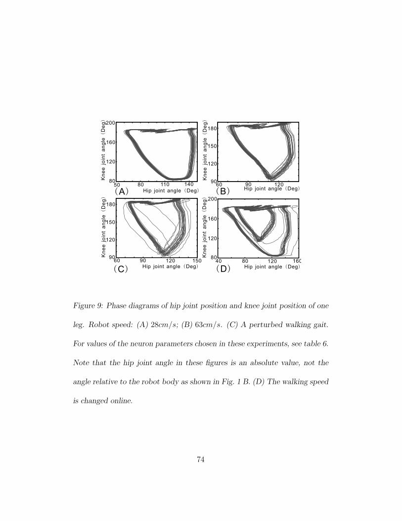
Figure 9: Phase diagrams of hip joint position and knee joint position of one
leg. Robot speed: (A) 28cm/s; (B) 63cm/s. (C) A perturbed walking gait.
For values of the neuron parameters chosen in these experiments, see table 6.
Note that the hip joint angle in these figures is an absolute value, not the
angle relative to the robot body as shown in Fig. 1 B. (D) The walking speed
is changed online.
74

Figure 10: The robot is climbing a shallow slope. The interval between any
two consecutive snapshots is 67 ms.
Figure 11: Model of the dynamics of our robot. Sizes and masses are the
same as those of the real robot.
75

Figure 12: Stable domain of the controller parameter, ΘES,h and GM,h. The
big area enclosed by the outer curve represents the range obtained with sim-
ulations in which fixed points are stable. The shaded area is the range of the
two parameters, in which stable gaits will appear in experiments performed
with the real robot. The maximum permitted value of GM,h is 2.95 (higher
values will destroy the motor of the hip joint). The two closed curves are
a manual, continuous interpolation of the discrete boundaries obtained in
simulations and real experiments, respectively.
76
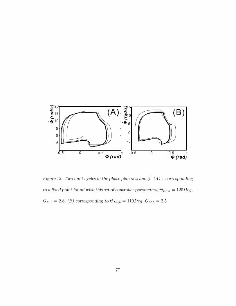
Figure 13: Two limit cycles in the phase plan of φ and φ. (A) is corresponding
to a fixed point found with this set of controller parameters, ΘES,h = 125Deg,
GM,h = 2.8, (B) corresponding to ΘES,h = 110Deg, GM,h = 2.5
77