a review of on-chip micro-evaporation: experimental...
TRANSCRIPT

Applied Energy 92 (2012) 147–161
Contents lists available at SciVerse ScienceDirect
Applied Energy
journal homepage: www.elsevier .com/locate /apenergy
A review of on-chip micro-evaporation: Experimental evaluation of liquid pumpingand vapor compression driven cooling systems and control
Jackson Braz Marcinichen a,⇑, Jonathan A. Olivier a, Vinicius de Oliveira b,1, John R. Thome a
a Laboratory of Heat and Mass Transfer (LTCM), École Polytechnique Fédérale de Lausanne (EPFL), Switzerlandb Automatic Control Laboratory (LA), École Polytechnique Fédérale de Lausanne (EPFL), Switzerland
a r t i c l e i n f o
Article history:Received 2 August 2011Received in revised form 13 October 2011Accepted 14 October 2011
Keywords:Data centerMicroprocessorOn-chip two-phase cooling cycleMicro-evaporatorController
0306-2619/$ - see front matter � 2011 Elsevier Ltd. Adoi:10.1016/j.apenergy.2011.10.030
⇑ Corresponding author. Tel.: +41 21 693 5894; faxE-mail address: [email protected] (J.B.
1 Tel.: +41 21 693 3845; fax: +41 21 693 2574.
a b s t r a c t
Thermal designers of data centers and server manufacturers are showing a greater concern regarding thecooling of the new generation data centers, which consume considerably more electricity and dissipatemuch more waste heat, a situation that is creating a re-thinking about the most effective cooling systemsfor the future beyond conventional air cooling of the chips/servers. A potential significantly better solu-tion is to make use of on-chip two-phase cooling, which, besides improving the cooling performance atthe chip level, also adds the capability to reuse the waste heat in a convenient manner, since higher evap-orating and condensing temperatures of the two-phase cooling system (from 60 to 95 �C) are possiblewith such a new ‘‘green’’ cooling technology. In the present project, two such two-phase cooling cyclesusing micro-evaporation technology were experimentally evaluated with specific attention being paidto (i) controllability of the two-phase cooling system, (ii) energy consumption and (iii) overall exergeticefficiency. The controllers were evaluated by tracking and disturbance rejection tests, which were shownto be efficient and effective. The average temperatures of the chips were maintained below the limit of85 �C for all tests evaluated in steady state and transient conditions. In general, simple SISO strategieswere sufficient to attain the requirements of control. Regarding energy and exergy analyses, the experi-mental results showed that both systems can be thermodynamically improved since only about 10% ofthe exergy supplied is in fact recovered in the condenser in the present setup.
� 2011 Elsevier Ltd. All rights reserved.
Contents
1. Introduction . . . . . . . . . . . . . . . . . . . . . . . . . . . . . . . . . . . . . . . . . . . . . . . . . . . . . . . . . . . . . . . . . . . . . . . . . . . . . . . . . . . . . . . . . . . . . . . . . . . . . . . . . 1482. Experimental facility . . . . . . . . . . . . . . . . . . . . . . . . . . . . . . . . . . . . . . . . . . . . . . . . . . . . . . . . . . . . . . . . . . . . . . . . . . . . . . . . . . . . . . . . . . . . . . . . . . 149
2.1. Cooling cycle proposals and general considerations . . . . . . . . . . . . . . . . . . . . . . . . . . . . . . . . . . . . . . . . . . . . . . . . . . . . . . . . . . . . . . . . . . . . 1492.2. Cooling cycle assembly and instrument uncertainties . . . . . . . . . . . . . . . . . . . . . . . . . . . . . . . . . . . . . . . . . . . . . . . . . . . . . . . . . . . . . . . . . . 150
3. Control system . . . . . . . . . . . . . . . . . . . . . . . . . . . . . . . . . . . . . . . . . . . . . . . . . . . . . . . . . . . . . . . . . . . . . . . . . . . . . . . . . . . . . . . . . . . . . . . . . . . . . . . 151
3.1. Liquid pumping cooling system . . . . . . . . . . . . . . . . . . . . . . . . . . . . . . . . . . . . . . . . . . . . . . . . . . . . . . . . . . . . . . . . . . . . . . . . . . . . . . . . . . . . 1513.1.1. Component controllers . . . . . . . . . . . . . . . . . . . . . . . . . . . . . . . . . . . . . . . . . . . . . . . . . . . . . . . . . . . . . . . . . . . . . . . . . . . . . . . . . . . . 1513.1.2. Dual SISO controller . . . . . . . . . . . . . . . . . . . . . . . . . . . . . . . . . . . . . . . . . . . . . . . . . . . . . . . . . . . . . . . . . . . . . . . . . . . . . . . . . . . . . . 153
3.2. Vapor compression cooling system . . . . . . . . . . . . . . . . . . . . . . . . . . . . . . . . . . . . . . . . . . . . . . . . . . . . . . . . . . . . . . . . . . . . . . . . . . . . . . . . . 155
3.2.1. Component controllers . . . . . . . . . . . . . . . . . . . . . . . . . . . . . . . . . . . . . . . . . . . . . . . . . . . . . . . . . . . . . . . . . . . . . . . . . . . . . . . . . . . . 1553.2.2. SISO–SIMO controller . . . . . . . . . . . . . . . . . . . . . . . . . . . . . . . . . . . . . . . . . . . . . . . . . . . . . . . . . . . . . . . . . . . . . . . . . . . . . . . . . . . . . 1574. Comparative analysis . . . . . . . . . . . . . . . . . . . . . . . . . . . . . . . . . . . . . . . . . . . . . . . . . . . . . . . . . . . . . . . . . . . . . . . . . . . . . . . . . . . . . . . . . . . . . . . . . . 158
4.1. Power consumption . . . . . . . . . . . . . . . . . . . . . . . . . . . . . . . . . . . . . . . . . . . . . . . . . . . . . . . . . . . . . . . . . . . . . . . . . . . . . . . . . . . . . . . . . . . . . 1594.2. Energy recovery. . . . . . . . . . . . . . . . . . . . . . . . . . . . . . . . . . . . . . . . . . . . . . . . . . . . . . . . . . . . . . . . . . . . . . . . . . . . . . . . . . . . . . . . . . . . . . . . . 1595. Conclusions. . . . . . . . . . . . . . . . . . . . . . . . . . . . . . . . . . . . . . . . . . . . . . . . . . . . . . . . . . . . . . . . . . . . . . . . . . . . . . . . . . . . . . . . . . . . . . . . . . . . . . . . . . 160Acknowledgements . . . . . . . . . . . . . . . . . . . . . . . . . . . . . . . . . . . . . . . . . . . . . . . . . . . . . . . . . . . . . . . . . . . . . . . . . . . . . . . . . . . . . . . . . . . . . . . . . . . 161References . . . . . . . . . . . . . . . . . . . . . . . . . . . . . . . . . . . . . . . . . . . . . . . . . . . . . . . . . . . . . . . . . . . . . . . . . . . . . . . . . . . . . . . . . . . . . . . . . . . . . . . . . . 161
ll rights reserved.
: +41 21 693 5960.Marcinichen).

Nomenclature
RomanASMV stepper motor valve aperture, %_Ed rate of exergy destruction due to irreversibilities within
the control volume, W_efi; _efe inlet and outlet flow exergies, J/kgG transfer function of the systemhi ME inlet specific enthalpy, kJ/kgho ME outlet specific enthalpy, kJ/kgKC PI proportional gainKI PI integral gainKP static gain of the system_m mass flow rate, kg/s_mi; _me inlet and outlet mass flow rate, kg/s
p position of the pole in the complex planPc condensing pressure, barPcsp set point of condensing pressure, barPi ME inlet pressure, barPo ME outlet pressure, bar_Qj heat transfer rate, WTi ME inlet temperature, �CTj instantaneous temperature, �CTI integral timeT0 dead state temperature, Ku system input_Wcv energy transfer rate by work, W_Winput pseudo chip input power, W
xo MEs’ outlet vapor qualityy system outputz position of the zero in the complex plan
GreekDTc difference in temperature between outlet water flow
and inlet working fluid flow in the condenser, �Ch transport delay, ss time constant, ssD desired closed-loop time constant, s
AcronymsCHF critical heat flux, W/cm2
COP coefficient of performanceCPU central processing unitEEV electric expansion valveHE heat exchangerHS heat spreaderiHEx internal heat exchangerLP liquid pumpLPR low pressure receiverLPS condenser liquid pump speed, rpmME micro-evaporatorMIMO multiple input multiple outputMMC multi-microchannel coolerPCV pressure control valveSMV stepper motor valveSIMO single input multiple outputSISO single input single outputTCV temperature control valveVC vapor compressor
148 J.B. Marcinichen et al. / Applied Energy 92 (2012) 147–161
1. Introduction
Under the current efficiency trends, the energy usage of datacenters in the US is estimated to become more than 100 billionkWh by 2011, which represents an annual energy cost of approxi-mately $7.4 billion [1]. With the introduction of a proposed carbontax in the US [2], the annual costs could become as high as $8.8 bil-lion by 2012, increasing annually. With the US having an annual in-crease of total electrical generation of approximately only 1.5%combined with the current growth rate of electrical energy by datacenters being between 10% and 20% per annum (driven now evenmore by smart phones), data centers potentially will consume all ofthe electrical energy produced by 2030 if current growth rates con-tinue! With air cooling of the servers in data centers accounting formost of the non-IT energy usage (up to 45% [3] of the total energyconsumption), this is the logical energy consumer that needs to beattacked to reduce its wasteful use.
Nowadays, the most widely used cooling strategy is refrigeratedair cooling of the data centers’ numerous servers. When makinguse of this solution, nevertheless, 40% or more of the refrigeratedair flow typically by-passes the racks of servers in data centersall together, according to articles presented at ASHRAE Winter An-nual Meeting at Dallas (January, 2007), while also ‘‘cooling’’ thou-sands of servers that are not even in operation. This massive wasteof energy motivates the search for a new ‘‘green’’ cooling solutionto the future generation of higher performance servers that con-sume much less energy for their cooling. One promising solutionis the application of on-chip two-phase cooling to dissipate thehigh heat flux densities of server CPU’s. The most promising work-ing fluids for these applications appear to be conventional refriger-ants, for instance HFC134a, as opposed to low pressure dielectriccoolants (such as FC-72) or water-cooling.
Hannemann et al. [4] proposed a pumped liquid multiphase cool-ing system (PLMC) to cool microprocessors and microcontrollers ofhigh-end devices such as computers, telecommunications switches,high-energy laser arrays and high-power radars. They emphasizedthe significant benefits of reduced pumping energy consumption,size and weight that were provided with the PLMC solution.
Mongia et al. [5] designed and built a small-scale refrigerationsystem applicable to a notebook computer, which included a mini-compressor, a microchannel condenser, a microchannel evaporatorand a capillary tube as the throttling device. COP’s in the order of3.7 were obtained, comparable with those obtained in modernhousehold refrigerators.
Trutassanawin et al. [6] designed, built and evaluated the per-formance of a miniature-scale refrigeration system (MSRS) suitablefor electronics cooling applications. It was concluded that,although COP’s in the order of 1.9–3.2 were obtained, a suitablecontrol strategy was required to improve its performance.
Zhang et al. [7] developed a set of active control strategies tosuppress the compressible flow boiling instabilities while alsomaintaining a reasonable electronic wall temperatures under tran-sient heat load changes. They found that efficient and effectivecontrol was obtained by making use of only two actuators; a valveprior to the heated channel and a supply pump. However, noexperimental evaluations of these systems were done to confirmtheir conclusions.
Zhou et al. [8] developed a steady-state model of a refrigera-tion system for high heat flux electronics cooling. The refrigera-tion system proposed consisted of multiple evaporators(microchannel technology), a liquid accumulator with an inte-grated heater, a variable speed compressor, a condenser and elec-tric expansion valves (EEVs). Their main conclusions were: (i) thesystem COP could be improved without compromising the critical
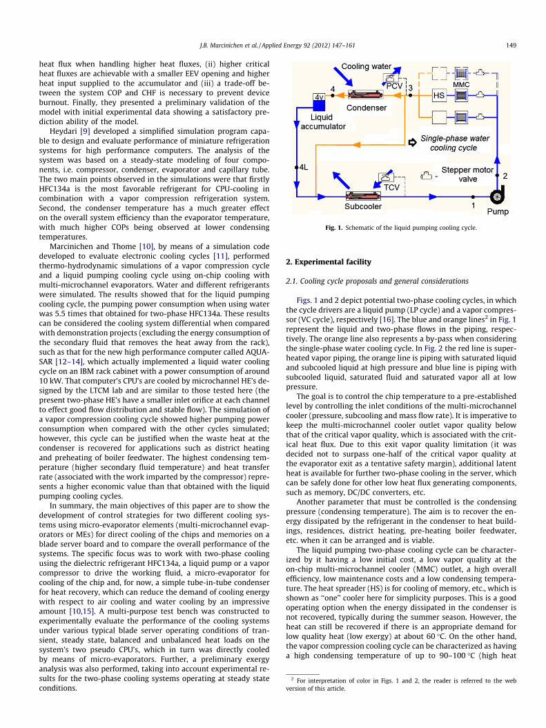
Fig. 1. Schematic of the liquid pumping cooling cycle.
2 For interpretation of color in Figs. 1 and 2, the reader is referred to the webversion of this article.
J.B. Marcinichen et al. / Applied Energy 92 (2012) 147–161 149
heat flux when handling higher heat fluxes, (ii) higher criticalheat fluxes are achievable with a smaller EEV opening and higherheat input supplied to the accumulator and (iii) a trade-off be-tween the system COP and CHF is necessary to prevent deviceburnout. Finally, they presented a preliminary validation of themodel with initial experimental data showing a satisfactory pre-diction ability of the model.
Heydari [9] developed a simplified simulation program capa-ble to design and evaluate performance of miniature refrigerationsystems for high performance computers. The analysis of thesystem was based on a steady-state modeling of four compo-nents, i.e. compressor, condenser, evaporator and capillary tube.The two main points observed in the simulations were that firstlyHFC134a is the most favorable refrigerant for CPU-cooling incombination with a vapor compression refrigeration system.Second, the condenser temperature has a much greater effecton the overall system efficiency than the evaporator temperature,with much higher COPs being observed at lower condensingtemperatures.
Marcinichen and Thome [10], by means of a simulation codedeveloped to evaluate electronic cooling cycles [11], performedthermo-hydrodynamic simulations of a vapor compression cycleand a liquid pumping cooling cycle using on-chip cooling withmulti-microchannel evaporators. Water and different refrigerantswere simulated. The results showed that for the liquid pumpingcooling cycle, the pumping power consumption when using waterwas 5.5 times that obtained for two-phase HFC134a. These resultscan be considered the cooling system differential when comparedwith demonstration projects (excluding the energy consumption ofthe secondary fluid that removes the heat away from the rack),such as that for the new high performance computer called AQUA-SAR [12–14], which actually implemented a liquid water coolingcycle on an IBM rack cabinet with a power consumption of around10 kW. That computer’s CPU’s are cooled by microchannel HE’s de-signed by the LTCM lab and are similar to those tested here (thepresent two-phase HE’s have a smaller inlet orifice at each channelto effect good flow distribution and stable flow). The simulation ofa vapor compression cooling cycle showed higher pumping powerconsumption when compared with the other cycles simulated;however, this cycle can be justified when the waste heat at thecondenser is recovered for applications such as district heatingand preheating of boiler feedwater. The highest condensing tem-perature (higher secondary fluid temperature) and heat transferrate (associated with the work imparted by the compressor) repre-sents a higher economic value than that obtained with the liquidpumping cooling cycles.
In summary, the main objectives of this paper are to show thedevelopment of control strategies for two different cooling sys-tems using micro-evaporator elements (multi-microchannel evap-orators or MEs) for direct cooling of the chips and memories on ablade server board and to compare the overall performance of thesystems. The specific focus was to work with two-phase coolingusing the dielectric refrigerant HFC134a, a liquid pump or a vaporcompressor to drive the working fluid, a micro-evaporator forcooling of the chip and, for now, a simple tube-in-tube condenserfor heat recovery, which can reduce the demand of cooling energywith respect to air cooling and water cooling by an impressiveamount [10,15]. A multi-purpose test bench was constructed toexperimentally evaluate the performance of the cooling systemsunder various typical blade server operating conditions of tran-sient, steady state, balanced and unbalanced heat loads on thesystem’s two pseudo CPU’s, which in turn was directly cooledby means of micro-evaporators. Further, a preliminary exergyanalysis was also performed, taking into account experimental re-sults for the two-phase cooling systems operating at steady stateconditions.
2. Experimental facility
2.1. Cooling cycle proposals and general considerations
Figs. 1 and 2 depict potential two-phase cooling cycles, in whichthe cycle drivers are a liquid pump (LP cycle) and a vapor compres-sor (VC cycle), respectively [16]. The blue and orange lines2 in Fig. 1represent the liquid and two-phase flows in the piping, respec-tively. The orange line also represents a by-pass when consideringthe single-phase water cooling cycle. In Fig. 2 the red line is super-heated vapor piping, the orange line is piping with saturated liquidand subcooled liquid at high pressure and blue line is piping withsubcooled liquid, saturated fluid and saturated vapor all at lowpressure.
The goal is to control the chip temperature to a pre-establishedlevel by controlling the inlet conditions of the multi-microchannelcooler (pressure, subcooling and mass flow rate). It is imperative tokeep the multi-microchannel cooler outlet vapor quality belowthat of the critical vapor quality, which is associated with the crit-ical heat flux. Due to this exit vapor quality limitation (it wasdecided not to surpass one-half of the critical vapor quality atthe evaporator exit as a tentative safety margin), additional latentheat is available for further two-phase cooling in the server, whichcan be safely done for other low heat flux generating components,such as memory, DC/DC converters, etc.
Another parameter that must be controlled is the condensingpressure (condensing temperature). The aim is to recover the en-ergy dissipated by the refrigerant in the condenser to heat build-ings, residences, district heating, pre-heating boiler feedwater,etc. when it can be arranged and is viable.
The liquid pumping two-phase cooling cycle can be character-ized by it having a low initial cost, a low vapor quality at theon-chip multi-microchannel cooler (MMC) outlet, a high overallefficiency, low maintenance costs and a low condensing tempera-ture. The heat spreader (HS) is for cooling of memory, etc., which isshown as ‘‘one’’ cooler here for simplicity purposes. This is a goodoperating option when the energy dissipated in the condenser isnot recovered, typically during the summer season. However, theheat can still be recovered if there is an appropriate demand forlow quality heat (low exergy) at about 60 �C. On the other hand,the vapor compression cooling cycle can be characterized as havinga high condensing temperature of up to 90–100 �C (high heat
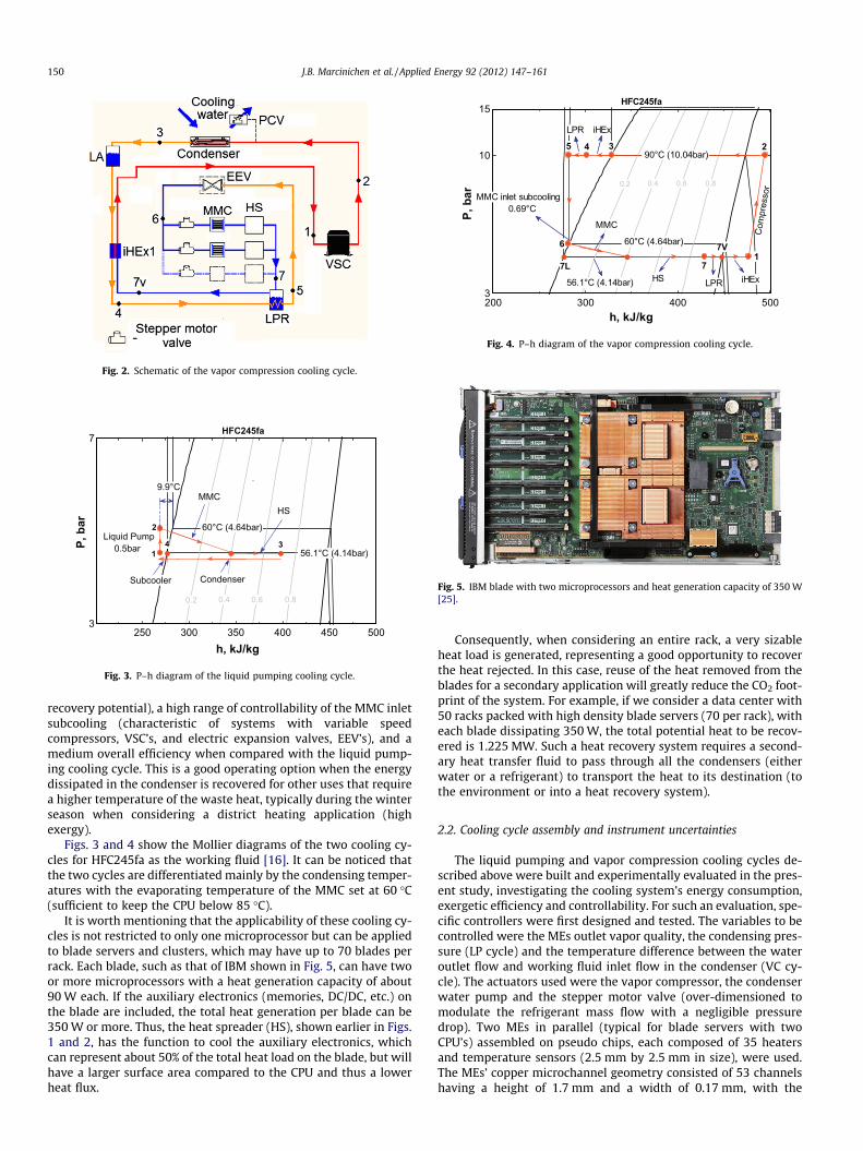
Fig. 2. Schematic of the vapor compression cooling cycle.
250 300 350 400 450 5003
7
h, kJ/kg
P, b
ar 60°C (4.64bar)
56.1°C (4.14bar)
HFC245fa
9.9°CMMC
HS
Liquid Pump0.5bar
0.2 0.4 0.6 0.8
CondenserSubcooler
13
2
4
Fig. 3. P–h diagram of the liquid pumping cooling cycle.
200 300 400 5003
10
15
h, kJ/kg
P, b
ar
90°C (10.04bar)
60°C (4.64bar)
56.1°C (4.14bar)
0.2 0.4 0.6 0.8
HFC245fa
1
245
6
7
7V
7L
LPR iHEx
iHEx
MMC
MMC inlet subcooling
LPR
HS
3
0.69°C
Com
pres
sor
Fig. 4. P–h diagram of the vapor compression cooling cycle.
Fig. 5. IBM blade with two microprocessors and heat generation capacity of 350 W[25].
150 J.B. Marcinichen et al. / Applied Energy 92 (2012) 147–161
recovery potential), a high range of controllability of the MMC inletsubcooling (characteristic of systems with variable speedcompressors, VSC’s, and electric expansion valves, EEV’s), and amedium overall efficiency when compared with the liquid pump-ing cooling cycle. This is a good operating option when the energydissipated in the condenser is recovered for other uses that requirea higher temperature of the waste heat, typically during the winterseason when considering a district heating application (highexergy).
Figs. 3 and 4 show the Mollier diagrams of the two cooling cy-cles for HFC245fa as the working fluid [16]. It can be noticed thatthe two cycles are differentiated mainly by the condensing temper-atures with the evaporating temperature of the MMC set at 60 �C(sufficient to keep the CPU below 85 �C).
It is worth mentioning that the applicability of these cooling cy-cles is not restricted to only one microprocessor but can be appliedto blade servers and clusters, which may have up to 70 blades perrack. Each blade, such as that of IBM shown in Fig. 5, can have twoor more microprocessors with a heat generation capacity of about90 W each. If the auxiliary electronics (memories, DC/DC, etc.) onthe blade are included, the total heat generation per blade can be350 W or more. Thus, the heat spreader (HS), shown earlier in Figs.1 and 2, has the function to cool the auxiliary electronics, whichcan represent about 50% of the total heat load on the blade, but willhave a larger surface area compared to the CPU and thus a lowerheat flux.
Consequently, when considering an entire rack, a very sizableheat load is generated, representing a good opportunity to recoverthe heat rejected. In this case, reuse of the heat removed from theblades for a secondary application will greatly reduce the CO2 foot-print of the system. For example, if we consider a data center with50 racks packed with high density blade servers (70 per rack), witheach blade dissipating 350 W, the total potential heat to be recov-ered is 1.225 MW. Such a heat recovery system requires a second-ary heat transfer fluid to pass through all the condensers (eitherwater or a refrigerant) to transport the heat to its destination (tothe environment or into a heat recovery system).
2.2. Cooling cycle assembly and instrument uncertainties
The liquid pumping and vapor compression cooling cycles de-scribed above were built and experimentally evaluated in the pres-ent study, investigating the cooling system’s energy consumption,exergetic efficiency and controllability. For such an evaluation, spe-cific controllers were first designed and tested. The variables to becontrolled were the MEs outlet vapor quality, the condensing pres-sure (LP cycle) and the temperature difference between the wateroutlet flow and working fluid inlet flow in the condenser (VC cy-cle). The actuators used were the vapor compressor, the condenserwater pump and the stepper motor valve (over-dimensioned tomodulate the refrigerant mass flow with a negligible pressuredrop). Two MEs in parallel (typical for blade servers with twoCPU’s) assembled on pseudo chips, each composed of 35 heatersand temperature sensors (2.5 mm by 2.5 mm in size), were used.The MEs’ copper microchannel geometry consisted of 53 channelshaving a height of 1.7 mm and a width of 0.17 mm, with the

Table 1Instruments uncertainty.
Instrument Range Uncertainty
Thermocouple at ME1 inlet (Ti) – �C 10–100 ±0.20Pressure transducer at ME1 inlet (Pi), bar 0–20 ±0.004Thermocouple at ME1 outlet (To) – �C 10–100 ±0.19Differential pressure transducer at ME1,
bar0–0.2 ±0.00058
Thermocouple at ME2 inlet (Ti) – �C 10–100 ±0.21Pressure transducer at ME2 inlet (Pi), bar 0–20 ±0.009Thermocouple at ME2 outlet (To) – �C 10–100 ±0.19Differential pressure transducer at ME2,
bar0–0.2 ±0.00069
Outlet vapor quality, % 0–100 ±0.5Power supply for pseudo chip 1 and 2, W 0–100 ±1.0% Of the
measured valueCoriolis mass flow meter, kg/h 0–108 ±0.05Power transducers of minicompressor, W 0–125 ±0.5% Of the
measured valuePower transducers of gear pump, W 0–1150 ±0.5% Of the
measured valuePower transducers of expansion valves,
W0–37.5 ±0.5% Of the
measured valueTurbine meter for secondary fluid at the
condenser, L/min0.0450–0.4280
±0.0023
J.B. Marcinichen et al. / Applied Energy 92 (2012) 147–161 151
spacing between channels being 0.17 mm (the same as in theAquasar project mentioned earlier). The effective ‘‘footprint’’ areaof the MEs is 12 mm length and 18 mm width. The pseudo chip/ME assembly has been extensively tested to study flow boiling heattransfer, two-phase pressure drops, hot spot cooling with non-uni-form heat fluxes, transient cooling, etc. by Costa-Patry et al.[17–19]. However, in the present work only uniform heat fluxeswere considered. HFC134a was tested as the working fluid andan oil free mini-compressor (supplied by Embraco of Joinville, Bra-zil) and a gear pump as drivers. It is important to highlight thecharacteristic ‘‘oil free’’ operation, which is mandatory for opera-tion of micro-evaporation cooling systems and is considered asan advantage of the new mini-compressor.
Table 1 shows the measuring instruments installed in theexperimental facility together with the uncertainties obtainedthrough calibration. The method proposed by Kline and McClintock[20] was used to determine the uncertainties. The uncertainty ofthe vapor quality is also shown and was determined by means ofthe propagation of errors due to the power transducer, Coriolismass flow meter, differential and absolute pressure transducersand K-type thermocouples. Eqs. (1) and (2) show the method usedto determine the ME outlet vapor quality. All thermodynamicproperties were determined from the Refprop [21] database. Final-ly, all data were captured by means of a data acquisition systemmaking use of the LabVIEW software. The data acquisition time,essential for the controllers’ design, was fixed at 0.75 s (each acqui-sition considered 850 samples per channel at a rate of 1000 Hz).
xo ¼ f ðho; poÞ determined from Refprop ð1Þ
ho ¼_W input
_mþhi; where hi ¼ f ðPi;TiÞ determined from Refprop
ð2Þ
3. Control system
3.1. Liquid pumping cooling system
3.1.1. Component controllersThe first controller developed was for modulating the con-
denser liquid pump speed (LPS), i.e. the water (secondary fluid)flow rate to the condenser, in order to maintain the condensing
pressure (Pc) at the set point value (Pcsp). The second controllerwas developed to control the MEs’ outlet vapor quality (xo), butwith the modulation of the stepper-motor-valve aperture (ASMV).This was achieved by deriving mathematical models capable ofrepresenting the dynamic behavior of the system under consider-ation by means of a system identification process and a PI structurethat was used for the controllers since the system showed low or-der dynamics.
The system identification, controller design and preliminaryevaluation by tracking tests, which are conventional steps in thedevelopment of new controllers, are presented below. In sequence,a deeper evaluation of the controllers operating together is shownfor what was named a dual SISO control strategy, which does notconsider the coupling effects between the controlled variables.Such a strategy was evaluated by disturbance rejection and flowdistribution tests; for the latter the effect of different heat loads ap-plied on the two micro-evaporators is investigated.
3.1.1.1. LPS controller: system identification and controller design.Fig. 6 illustrates the block diagram of the first control loop, wherethe condensing pressure (Pc) is the controlled variable (Pcsp is theset point) and the condenser liquid pump speed (LPS) is the manip-ulated variable.
The system identification process has the objective of deriving amathematical model capable of representing the dynamic behaviorof the system. A linear first-order model with delay was used tocorrelate Pc with the LPS variations. The condensing pressurewas measured with a calibrated pressure transducer at the inletof the condenser. For such a system, the pressure drop betweenthe inlet of MEs and inlet of condenser is negligible (<0.03 bar),so the condensing pressure controller can also be considered asan evaporating pressure controller. Eqs. (3) and (4) show the modelin the time and Laplace domains, respectively:
sdyðtÞdtþ yðtÞ ¼ Kpuðt � hÞ ð3Þ
GðsÞ ¼ yðsÞuðsÞ ¼
Kpee�hs
ssþ 1ð4Þ
The input (u) and output (y) parameters are LPS and Pc, respec-tively, while G is the transfer function, s the system time constant,KP the gain and h the transport delay.
The model parameters were obtained by varying the LPS from1620 rpm to 1800 rpm (step response experiment, viz. Fig. 7).The cycle’s liquid pump speed, the water temperature (secondaryfluid) at the inlet of condenser, the SMV’s aperture and the heatload on the MEs were maintained at 3000 rpm, 40 �C, 25%, and90 W for ME1 and 75 W for ME2, respectively. These operatingconditions are from now on referred to as the standard conditions.
It is important to mention that during the initial tests it was ob-served that the subcooler was redundant for this cycle and level ofheat load investigated. This was due to the heat losses in the pip-ing, which ensured that there was always enough subcooling atthe inlet of the liquid pump and micro-evaporators. Such a situa-tion might not be the same for the case of better piping insulationand higher heat load, as for an entire blade center (e.g. IBM bladecenter QS22 with a heat load of about 5000 W). The subcoolingat the inlet manifold of the MEs in all evaluations considered in thiswork remained between 2 and 8 K, avoiding the necessity for spe-cial controllers to avoid saturation conditions (that is, unwantedvapor in the inlet header of ME1 and ME2), which would otherwisejeopardize the MEs’ performance by creation of flowmaldistribution.
The model parameters KP, s and h were estimated in order tominimize the square error between the model predictions and

-+ -+ --+ ControllerCooling System
Pcsp PcLPS
Fig. 6. LPS controller.
16.60
16.64
16.68
16.72
16.76
16.80
16.84
1550
1600
1650
1700
1750
1800
1850
0 100 200 300 400 500C
onde
nsin
g pr
essu
re, b
ar
Pum
p sp
eed,
rpm
Time, s
LPS
Pc
Fig. 7. LPS – model identification. (For interpretation of the references to colour inthis figure legend, the reader is referred to the web version of this article.)
16.60
16.64
16.68
16.72
16.76
16.80
16.84
0 100 200 300 400 500
Con
dens
ing
pres
sure
, bar
Time, s
Pc
Pc,model
Fig. 8. LPS – experimental vs. prediction. (For interpretation of the references tocolour in this figure legend, the reader is referred to the web version of this article.)
16.70
16.75
16.80
16.85
16.90
16.95
17.00
17.05
17.10
0 1000 2000 3000 4000 5000 6000 7000
Pres
sure
, bar
Time, s
Experimental
Set point
Step 1
Step 2
Step 3
Step 4
Step 5
Step 6
59.96ºC
59.81ºC
Fig. 9. Pc variation. (For interpretation of the references to colour in this figurelegend, the reader is referred to the web version of this article.)
152 J.B. Marcinichen et al. / Applied Energy 92 (2012) 147–161
the experimental data. For this controller KP, s and h wereestimated as �0.8 mbar/rpm, 90.85 s and 2.59 s, respectively.Figs. 7 and 8 depict part of the identification tests, showing thePc response to a step change in the LPS and also the Pc model pre-dictions against the experimental data.
As mentioned beforehand, the PI structure was selected forthis study. Eq. (5) shows the PI controller transfer function in theLaplace domain:
CðsÞ ¼ KC 1þ 1TIs
� �ð5Þ
The PI controller was designed using the method proposed by[22], which is based on linear programming. It was computed toguarantee a phase margin of 30�, a gain margin of 2 and a crossoverfrequency two times larger than in an open loop. The TI (integraltime) and KC (proportional) parameters were calculated as90.85 s and �9816 bar/rpm, respectively.
3.1.1.2. Controller evaluation. Tracking tests were carried out withthe experimental apparatus running under the standard operatingconditions to evaluate the controller performance. Figs. 9 and 10show the results for five steps in the pressure set point between16.8 bar and 17.0 bar for the LPS controller. As can be noticed,the controller increased or decreased the liquid pump speed, in re-sponse to a decrease or increase in the pressure set point value.
The results showed that the controller is effective and efficientto track the set point of pressure in a short time (ffi3.5 min afterstep 6, viz. Fig. 11) with a maximum overshoot in the condensingtemperature of only about 0.16 �C (viz. Fig. 9).
3.1.1.3. SMV controller: system identification and controller’s designand evaluation. The controller developed for the MEs’ outlet vaporquality considered the SMV as the actuator. The vapor quality ofthe flow after the outlet of the MEs was used for control. It is worthmentioning that this variable has a considerable effect on the per-formance of the ME [23], and as a consequence on the overall sys-tem. Therefore, for safe operating reasons, such a controller mustavoid the critical vapor quality, a condition where the pseudo chipscould be damaged due to dryout occurring. Fig. 12 illustrates thecontroller’s block diagram.
The system identification was developed considering the stan-dard conditions as a starting point and a change in SMV apertureof 2% each 10 s between 22% and 40% of aperture. The average ofvapor quality for the last 5 s of each change was considered asthe value for each aperture, i.e. the values shown in Fig. 13. It isimportant mentioning that the vapor quality was calculated/deter-mined for each acquisition time by an energy balance enclosing theMEs, where the heat load, mass flow rate and inlet/outlet pressuresand temperatures required for this calculation, were measuredwith calibrated transducers.
During the system identification it was observed that smallchanges in the aperture resulted in a fast response (2 s . . . 3 s) inthe exit vapor quality, as can be seen in Fig. 14. Thus, the modelof the system was approximated by its static gain (KP), which var-ied nonlinearly with the SMV aperture change, as can be seenbelow:
Kp ¼@X
@SMV¼ �7:8� 10�6SMV4 þ 10:4� 10�4SMV3 � 5:2� SMV2
þ 1:16SMV� 9:63 ð6Þ
Therefore, a gain-scheduled PI controller was developed whosegain was a function of the SMV aperture. That is, the closed-looptransfer function was represented by Eq. (7), where the time con-stant (s) is given by Eq. (8):
HðsÞ ¼ xo
xo;sp¼
KcKi
sþ 1 fzerossð1þKc �KpÞ
Ki �Kpþ 1 fpoles
ð7Þ

500
1000
1500
2000
2500
3000
0 1000 2000 3000 4000 5000 6000 7000
Liqu
id P
ump
Spee
d, rp
m
Time, s
Step 1
Step 2
Step 3 Step 4
Step 5
Step 6
Fig. 10. LPS variation.
16.70
16.75
16.80
16.85
16.90
16.95
17.00
17.05
17.10
5000 5200 5400 5600 5800 6000
Pres
sure
, bar
Time, s
Experimental
Set pointStep 6
3.5 min
Fig. 11. Pc variation for step 6. (For interpretation of the references to colour in thisfigure legend, the reader is referred to the web version of this article.)
-+ -+ --+ Controller Cooling System
xo,sp ASMV xo
Fig. 12. SMV controller.
0
0.1
0.2
0.3
0.4
0.5
0.6
20 25 30 35 40 45
Out
let v
apor
qua
lity,
-
SMV aperture
Fig. 13. System identification: xo vs. SMV aperture.
22
24
26
28
30
32
0.15
0.20
0.25
0.30
0.35
0.40
15 25 35 45 55
SMV
aper
ture
, %
Vapo
r qua
lity,
-
Time, s
Outlet vapour qualitySMV aperture
3 s
Fig. 14. System identification: response time of exit vapor quality by changing theSMV aperture.
J.B. Marcinichen et al. / Applied Energy 92 (2012) 147–161 153
s ¼ 1þ Kc � Kp
Ki � Kpð8Þ
Defining sD as the desired closed-loop time constant, and C as aparameter relating the closed-loop pole (p) and zero (z) such thatp = C.z, Eqs. (9) and (10) were obtained for the integral and propor-tional constants, i.e. KI and KC:
KC ¼1
ðC � 1Þ � Kpð9Þ
KI ¼C
C � 1� 1sD � Kp
¼ TI
KCð10Þ
The gains KI and KC of the controller are functions of the staticgain of the system KP and are updated during runtime. C and sD
can be seen as tuning parameters, which were experimentally ad-justed for 15 and 5 s, respectively. Moreover, an anti-wind up strat-egy was implemented to reduce the accumulated integral error ofthe controller when the output of the controller moved outside theSMV’s range (22–40% of aperture). It is worth highlighting thatother techniques to design the gain-scheduled controller could alsobe used, for example, the method proposed in [24].
Fig. 15 shows the outlet vapor quality tracking test, where it canbe seen that the controller reacted fairly quickly for the 4 stepsconsidered. In the worst case, the controller took about 30 s to sta-bilize the system; however only a small overshoot was observed,i.e. a maximum of 1.5% in vapor quality. Finally, it can be concludedthat the controller was efficient and effective for the actual appli-cation, showing a small overshoot and settling time.
3.1.2. Dual SISO controllerThe dual SISO control strategy was derived from the two indi-
vidual controllers, as illustrated in the block diagram of Fig. 16.This allowed the simultaneous control of Pc and xo to match thethermal load with the cooling capacity for the condensing temper-ature and vapor quality desired.
Disturbance rejection and flow distribution tests were per-formed with the experimental apparatus running under a standardoperating condition to evaluate the controllers’ performance. Inthese tests, after the apparatus was in a steady-state regime, theinput power on the pseudo chips (heat load on the MEs) waschanged periodically for a constant period of time between twolevels for the disturbance rejection tests and changed to differentlevels until the steady state condition was established for the flowdistribution tests, as will be shown below.
3.1.2.1. Heat load disturbance rejection. The integrated controller ordecentralized control structure was first evaluated by consideringthe standard conditions at the beginning of the test, and a set pointof condensing pressure (Pcsp) and outlet vapor quality of 16.8 barand 22%, respectively. The performance of the control strategiesregarding disturbance rejections was evaluated by periodicallychanging the heat load on the micro-evaporators. As the heat loadchanged, so did the condensing pressure and vapor quality distur-bances, which were detected automatically by the controllers.These in turn increased or decreased the LPS and SMV apertureto maintain the pressure and vapor quality at the set point.

0.15
0.17
0.19
0.21
0.23
0.25
0.27
0.29
0.31
0 100 200 300 400 500 600
Out
let v
apor
qua
lity,
-
Time, s
Experimental
Set point
Step 1
Step 2
Step 3
Step 4
30 s
Fig. 15. Outlet vapor quality tracking test. (For interpretation of the references tocolour in this figure legend, the reader is referred to the web version of this article.)
Pcsp LPS Pc
xo,sp ASMV xo
-+
Controller
ControllerCoolingSystem
-+
Fig. 16. The dual SISO controller.
10 15 20 25 30 35 4063
64
65
66
67
68
69
70
71
50
56
62
68
74
80
86
92
98
Time [s]
Tem
pera
ture
[ºC
]
Average temperature pseudo chip 2Average temperature pseudo chip 2Average temperature pseudo chip 1Average temperature pseudo chip 1
Pseudo chip 1 and 2
Inpu
t pow
er [W
]
Input power pseudo chip 1Input power pseudo chip 1
Input Power pseudo chip 2Input Power pseudo chip 2
Fig. 17. Heat load disturbance and pseudo chip temperatures. (For interpretation ofthe references to colour in this figure legend, the reader is referred to the webversion of this article.)
10 15 20 25 30 35 40 45 50 55 60
0.15
0.20
0.25
0.30
0.35
28
32
36
40
44
Time [s]
Vapo
r qua
lity
[-]Outlet vapor quality - Junction
Set point
SMV
aper
ture
[%]SMV apertureSMV aperture
±0.05
Fig. 18. Outlet vapor quality and SMV controller. (For interpretation of thereferences to colour in this figure legend, the reader is referred to the web versionof this article.)
0 100 200 300 400 500 60016.74
16.76
16.78
16.80
16.82
16.84
16.86
1000
1200
1400
1600
1800
2000
2200
Time [s]
Pres
sure
[bar
]
Set pointLi
quid
pum
p sp
eed
[rpm
]Liquid pump speed
Condensing pressure
Offset
Fig. 19. Condensing pressure and LPS controller. (For interpretation of thereferences to colour in this figure legend, the reader is referred to the web versionof this article.)
154 J.B. Marcinichen et al. / Applied Energy 92 (2012) 147–161
The heat load on ME1 and ME2 were changed between 90 Wand 75 W and 75 W and 60 W, respectively, considering a periodicdisturbance time of 1.4 s. Fig. 17 shows the input power distur-bance on the pseudo chips and the effect on the average tempera-ture of each chip. This temperature was obtained by averaging thetemperature from 11 well distributed sensors on each chip. It canbe observed that there was a maximum temperature variation of1.5 �C, which can be considered to be acceptable when comparedto the temperature gradient along the chip for on-chip single-phase cooling using water (about 2–3 K [12–14]).
Figs. 18 and 19 show the controllers’ reaction under the situa-tion of a disturbance. It can be seen that the SMV controller wasable to maintain the exit vapor quality to within ±5% of the setpoint. What is important to observe is that the controller was effec-tive, i.e. it showed fast response for the induced disturbance and noinstability was observed.
The LPS controller (viz. Fig. 19) showed an initial offset whenthe heat load disturbance started, which represents a condensingtemperature deviation of only 0.05 bar or 0.1 �C (it also representsa very small evaporating temperature variation) and it can be seenthat the controller was able to reset the offset after about 2.5 min.Once again the controller proved to be effective and efficient inmaintaining the set point.
3.1.2.2. Flow distribution for non-uniform heat load. To evaluate theeffect of a non-uniform heat load applied to the two MEs on theflow distribution and, consequently, on the pseudo chips’ temper-ature and performance of the controllers, tests were developed fordifferent heat loads between 30 W and 90 W and set points of out-let vapor quality between 15% and 22%. A total of eight differentcombinations of such heat loads and three outlet vapor qualitieswere evaluated, as can be seen in Figs. 20 and 21.
The tests started with the standard conditions, a set point of con-densing pressure and outlet vapor quality of 16.8 bar and 22%, andheat loads on ME1 and ME2 of 90 W and 75 W, respectively. Sevensteps of heat load combinations were then imposed, with the lastone considering three different vapor quality set points; 22%, 18%and 15%. The steady state condition was obtained before eachnew change in heat load or set point of vapor quality. Figs. 21
and 22 show the results obtained for the average temperature onthe pseudo chips, the MEs’ outlet vapor qualities and the SMVaperture (action of the controller).

0 500 1000 1500 2000 2500 30000.10
0.15
0.20
0.25
0.30
0.35
0.40
20
24
28
32
36
40
44
Time [s]
Vapo
r qua
lity
[-]
Outlet vapor quality - Junction
Set point
SMV
aper
ture
[%]SMV apertureSMV aperture
Step 7
≈ 30 s
Fig. 22. Outlet vapor quality and SMV aperture. (For interpretation of thereferences to colour in this figure legend, the reader is referred to the web versionof this article.)
16.83
16.86
2000
2400
2800
] [rpm
]Step 1 Step 2 Step 4 Step 6
J.B. Marcinichen et al. / Applied Energy 92 (2012) 147–161 155
Firstly, it can be seen that the SMV controller was effective andefficient in controlling the outlet vapor quality under differentconditions of heat load and set points of exit vapor quality. Thecontroller proved to be very fast in reaching the steady statecondition, with the maximum transient time observed to be about30 s in step 7, all the while maintaining the pseudo CPU averagetemperatures well below 85 �C (typically upper operational limit).
Regarding the pseudo chips’ temperatures (viz. Fig. 21), thefollowing aspects were observed
(a) For the same heat load, step 2, the average temperature ofboth pseudo chips was the same, i.e. about 67 �C. Thisimplies that the distributors (piping) before and after theMEs were well designed and that both MEs have the samemass flow rate.
(b) The maximum temperature difference observed was, asexpected, in step 7, which considered 90 W on chip 1 and30 W on chip 2. A difference of 14.5 �C was obtained, wherechip 1 reached a temperature of 75 �C vs. 60.5 �C on chip 2.Despite this difference, the limit of 85 �C is still very far away.
(c) The chips’ temperature difference and the absolute temper-atures were reduced when the set point of the outlet vaporquality was reduced. A difference of 11.5 �C and a tempera-ture of 71.5 �C were obtained for chip 1 when the outletvapor quality set point was reduced to 15%.
0 500 1000 1500 2000 2500 300020
30
40
50
60
70
80
90
100
Time [s]
Inpu
t pow
er [W
]
Pseudo chip 1Pseudo chip 1Pseudo chip 2Pseudo chip 2
Step 1
Step 2
Step 3
Step 4
Step 5
Step 6
Step 7
Fig. 20. Different heat loads on the MEs. (For interpretation of the references tocolour in this figure legend, the reader is referred to the web version of this article.)
0 500 1000 1500 2000 2500 300056
60
64
68
72
76
80
Time [s]
Tem
pera
ture
[ºC
]
Average temperature pseudo chip 2Average temperature pseudo chip 2Average temperature pseudo chip 1Average temperature pseudo chip 1
Step 1
Step 2Step 3
Step 4
Step 5
Step 6
Step 7
xo = 22% x o =
18%
x o =
15%
Fig. 21. Average temperature on the pseudo chips. (For interpretation of thereferences to colour in this figure legend, the reader is referred to the web version ofthis article.)
0 500 1000 1500 2000 2500 300016.65
16.68
16.71
16.74
16.77
16.80
0
400
800
1200
1600
Time [s]
Pres
sure
[bar
Set pointSet point
Liqu
id p
ump
spee
d
Liquid pump speedLiquid pump speed
Condensing pressureCondensing pressure
Step 3Step 5
Step 7
≈5 min
≈0.1 oC
Fig. 23. Condensing pressure and LPS. (For interpretation of the references to colourin this figure legend, the reader is referred to the web version of this article.)
Fig. 23 shows the effect of a non-uniform heat load on the LPScontroller. It can be seen that for all ranges of heat loads investi-gated, the controller was able to control and stabilize the condens-ing pressure at the set point. The maximum disturbance observedwas stabilized after 5 min and provoked an overshoot of only 0.1 �Cin the condensing temperature.
Finally, it can be highlighted that the dual SISO strategy provedto be a simple and effective way of controlling the condensingpressure and vapor quality while maintaining the pseudo chipswithin a safe operating range. The coupling effect between thetwo controllable variables was not strong, in other words the con-trollers have low interaction effects, implying that it was not nec-essary to apply a more complex centralized MIMO controller.
3.2. Vapor compression cooling system
3.2.1. Component controllersFor the vapor compression cooling system, alternative control
strategies were adopted due to its cooling cycle concept being dif-ferent. In this system, the objective is not only to cool the pseudochips but also to recover the energy removed in the condenser,since a higher condensing temperature is possible to be obtained(higher exergy thus available). From this point of view, the differ-ence in temperature between outlet water flow and inlet workingfluid flow in the condenser (DTc) and the MEs’ outlet vapor qualitywere defined as the variables to be controlled. The manipulated

0 1000 2000 3000 4000 5000 6000 7000 8000 90000.3
0.4
0.5
0.6
0.7
Time [s]
Out
let v
apor
qua
lity
[-]
ExperimentalSet pointSet point
Step 1
Step 2
Step 3
Step 4
Step 5
Step 6
Fig. 24. Outlet vapor quality tracking test. (For interpretation of the references tocolour in this figure legend, the reader is referred to the web version of this article.)
156 J.B. Marcinichen et al. / Applied Energy 92 (2012) 147–161
variables were, for the former, the LPS and for the latter the SMVaperture and the mini-compressor stroke length. It is worth men-tioning that preliminary evaluations for the LPS controlling thecondensing pressure were developed, as used in the liquid pump-ing cooling system. However, this variable showed a strong cou-pling with the outlet vapor quality, which provoked instabilitiesin the system when the controllers were operated together.
The SMV was used as an expansion device (EEV in Fig. 2) andalso as an actuator to control the outlet vapor quality together withthe mini-compressor. The results obtained in this work, as will beshown, proved that since the system is well designed and con-trolled, a SMV for each ME is not necessary, as was initially pro-posed by [16] and schematically given in Fig. 2, i.e. only one SMVor EEV is sufficient to operate as an expansion device and actuatorfor the outlet vapor quality controller. It should be mentioned thatthis is probably only valid when two MEs are considered (only oneblade), with a more general statement only being valid once a com-plete blade center has been evaluated. The mini-compressor is alinear oil-free compressor capable of modulating the volumetricdisplacement, here defined as the stroke, according to the manu-facturer’s scale, between zero and ten.
Regarding the thermodynamic conditions at the inlet of themini-compressor and MEs, all tests presented in this work showedsuperheating and subcooling conditions, respectively. The valuesremained between 1 K and 10 K, and in the same way as was ob-served in the previous system, special controllers were not re-quired to avoid saturation conditions. The reason is partlyassociated with the performance obtained by the iHEx and LPRcomponents (viz. Fig. 2). As will be discussed below, they demon-strated a high exergetic efficiency and consequently ensured theconditions mentioned beforehand.
3.2.1.1. SMV and mini-compressor controllers. System identification,controller design and reference tracking evaluation were done, asfor the previous system. To control the MEs’ outlet vapor quality,the SMV aperture and the mini-compressor stroke were used asmanipulating variables. Therefore, two PI controllers were designedindependently. The SMV controller used the same strategy, i.e. again-scheduling PI controller whose parameters are actualized/up-dated for each acquisition time. The relationship between themanipulated and the controlled variables can be considered static,which is a function of the SMV and is given by (static gain KP):
Kp ¼@X
@SMV¼ 3:5� 10�2SMV3 � 1:1SMV2 þ 10:9SMV� 36:2 ð11Þ
The gains of the controller are a function of the gain KP accord-ing to Eqs. (9) and (10). The desired closed-loop time constant wasadjusted to sD = 15 s, the constant C = 35 and the anti-wind up setto 0.5. Due to the SMV operating as an expansion device, the rangeof operation was limited to between 6.5% and 9% of aperture.
For the mini-compressor controller, the transfer function ob-tained from the system identification is given by:
GðsÞ ¼ yðsÞuðsÞ ¼
�0:0573e�0:0741s
8:23sþ 1ð12Þ
Using the linear programming method proposed in [22] andconsidering a phase margin of 60�, a gain margin of 2 and acrossover frequency twice as large as in the open loop, the mini-compressor’s PI parameters, i.e. KC and TI, were determined as�34.3%/stroke and 8.23 s, respectively.
3.2.1.2. LPS controller. To control the difference of temperature be-tween outlet water flow and inlet working fluid flow in the con-denser, i.e. DTc, the LPS was used as the manipulating variable.
The transfer function obtained from the system identification is gi-ven by Eq. (13), and the LPS controller parameters adjusted were82.04 �C/rpm and 33.76 s, respectively for KC and TI. The same cri-teria and method used for the design of the mini-compressor con-troller was used:
GðsÞ ¼ yðsÞuðsÞ ¼
0:0234e�0:01s
33:76sþ 1ð13Þ
3.2.1.3. Controller evaluation. A standard condition was defined tostart each evaluation, i.e., mini-compressor stroke of 4, SMV aper-ture of 7.7%, LPS of 1100 rpm, inlet water temperature in the con-denser of 14 �C and input heat loads of 75 W, 75 W and 150 W onpseudo chips 1 and 2, and on the post heater wrapped on the pip-ing after the MEs (HS in the Fig. 2), respectively.
The post heater was necessary to guarantee superheated condi-tions at the inlet of the VSC and subcooled liquid at the inlet of theMEs. The post heater simulates the auxiliary electronics describedbeforehand and in [16]. A fixed value of 125 W was used, which,combined with the input power on the pseudo chips, added upto a total heat load of about 290 W, which is equivalent to the heatload associated with IBM’s QS22 blade.
Figs. 24 and 25 show the results for the MEs’ outlet vapor qual-ity tracking test, where DTc was set to the value of 15 K. The stan-dard condition was defined as the starting point and six steps ofvapor quality from 40% to 60% were investigated.
The outlet vapor quality proved to be well controlled by the twoactuators operating together. It can be said that a negligible overshootwas observed and the controllers, mini-compressor and SMV, are effi-cient and effective in tracking the outlet vapor quality since no insta-bilities were observed in the outlet vapor quality. In the worst case, i.e.step 3, the controller took about 60 s to stabilize the system.
An anomalous operation was observed in the controller of themini-compressor, as can be seen in Fig. 25. When the mini-com-pressor controller tried to increase the stroke, defined by the strokecontroller, the actual stroke or stroke measured did not respond asdefined by the controller. Such a situation was observed duringsteps 3, 4 and 5, and certainly has some negative effect in the per-formance of the controller, which was not observed in the presentwork probably due to the SMV controller compensating this defi-ciency. A possible reason is that the mini-compressor was not de-signed for such extreme operating conditions (evaporation ofabout 60 �C and condensation of about 80 �C compared to its nor-mal design operating condition of about 5 �C and 45 �C).
0 1000 2000 3000 4000 5000 6000 7000 8000 90000.3
0.4
0.5
0.6
0.7
0.00
2.25
4.50
6.75
9.00
Time [s]
Out
let v
apor
qua
lity
[-]
xo set point
Step 1
Step 2
Step 3Step 4
Step 5
Step 6
Min
icom
pres
sor s
trok
e [%
] or
S
MV
aper
ture
[%]
Stroke controllerStroke measured
SMV apertureSMV aperture
Fig. 25. SMV and minicompressor actuators. (For interpretation of the references tocolour in this figure legend, the reader is referred to the web version of this article.)
J.B. Marcinichen et al. / Applied Energy 92 (2012) 147–161 157
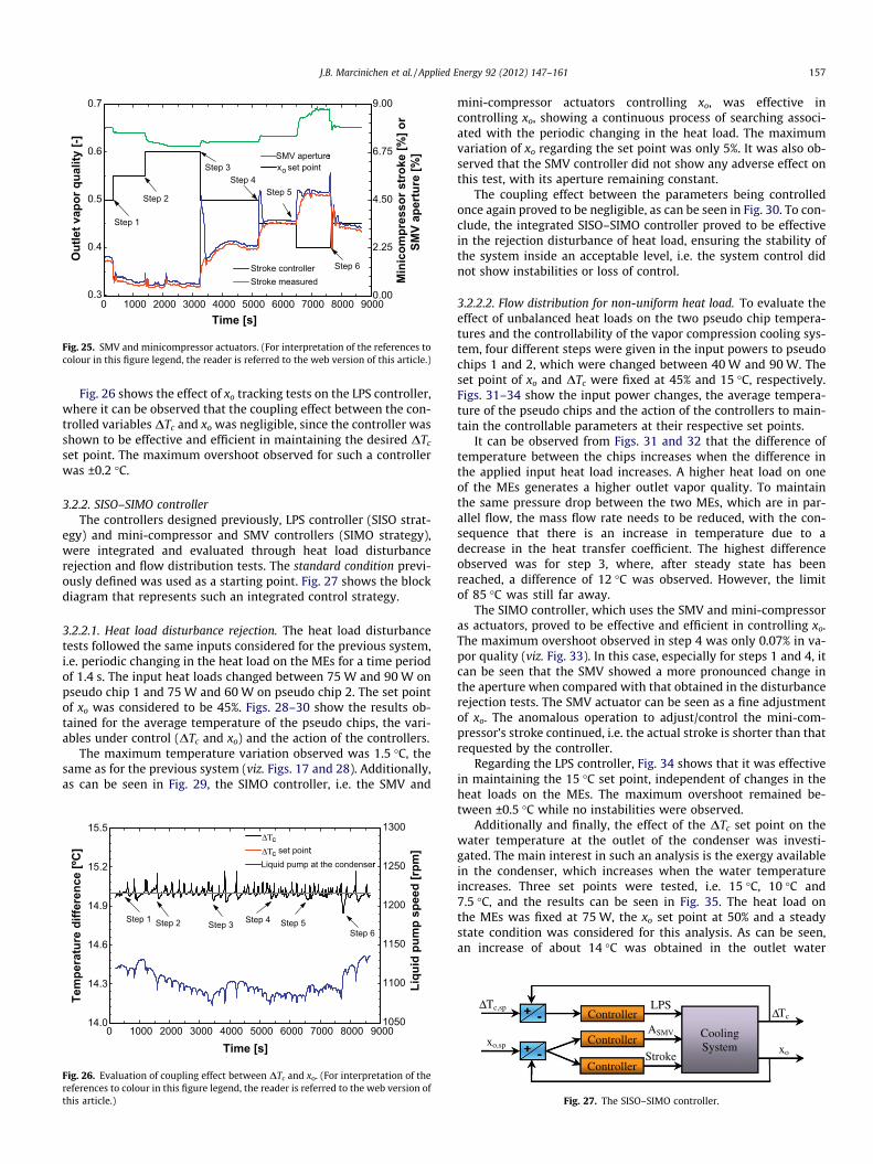
Fig. 26 shows the effect of xo tracking tests on the LPS controller,where it can be observed that the coupling effect between the con-trolled variables DTc and xo was negligible, since the controller wasshown to be effective and efficient in maintaining the desired DTc
set point. The maximum overshoot observed for such a controllerwas ±0.2 �C.
3.2.2. SISO–SIMO controllerThe controllers designed previously, LPS controller (SISO strat-
egy) and mini-compressor and SMV controllers (SIMO strategy),were integrated and evaluated through heat load disturbancerejection and flow distribution tests. The standard condition previ-ously defined was used as a starting point. Fig. 27 shows the blockdiagram that represents such an integrated control strategy.
3.2.2.1. Heat load disturbance rejection. The heat load disturbancetests followed the same inputs considered for the previous system,i.e. periodic changing in the heat load on the MEs for a time periodof 1.4 s. The input heat loads changed between 75 W and 90 W onpseudo chip 1 and 75 W and 60 W on pseudo chip 2. The set pointof xo was considered to be 45%. Figs. 28–30 show the results ob-tained for the average temperature of the pseudo chips, the vari-ables under control (DTc and xo) and the action of the controllers.
The maximum temperature variation observed was 1.5 �C, thesame as for the previous system (viz. Figs. 17 and 28). Additionally,as can be seen in Fig. 29, the SIMO controller, i.e. the SMV and
0 1000 2000 3000 4000 5000 6000 7000 8000 900014.0
14.3
14.6
14.9
15.2
15.5
1050
1100
1150
1200
1250
1300
Time [s]
Tem
pera
ture
diff
eren
ce [º
C]
Liqu
id p
ump
spee
d [r
pm]
ΔΤcΔΤc
Liquid pump at the condenserLiquid pump at the condenserΔΤc set pointΔΤc set point
Step 1 Step 2 Step 3 Step 4 Step 5Step 6
Fig. 26. Evaluation of coupling effect between DTc and xo. (For interpretation of thereferences to colour in this figure legend, the reader is referred to the web version ofthis article.)
mini-compressor actuators controlling xo, was effective incontrolling xo, showing a continuous process of searching associ-ated with the periodic changing in the heat load. The maximumvariation of xo regarding the set point was only 5%. It was also ob-served that the SMV controller did not show any adverse effect onthis test, with its aperture remaining constant.
The coupling effect between the parameters being controlledonce again proved to be negligible, as can be seen in Fig. 30. To con-clude, the integrated SISO–SIMO controller proved to be effectivein the rejection disturbance of heat load, ensuring the stability ofthe system inside an acceptable level, i.e. the system control didnot show instabilities or loss of control.
3.2.2.2. Flow distribution for non-uniform heat load. To evaluate theeffect of unbalanced heat loads on the two pseudo chip tempera-tures and the controllability of the vapor compression cooling sys-tem, four different steps were given in the input powers to pseudochips 1 and 2, which were changed between 40 W and 90 W. Theset point of xo and DTc were fixed at 45% and 15 �C, respectively.Figs. 31–34 show the input power changes, the average tempera-ture of the pseudo chips and the action of the controllers to main-tain the controllable parameters at their respective set points.
It can be observed from Figs. 31 and 32 that the difference oftemperature between the chips increases when the difference inthe applied input heat load increases. A higher heat load on oneof the MEs generates a higher outlet vapor quality. To maintainthe same pressure drop between the two MEs, which are in par-allel flow, the mass flow rate needs to be reduced, with the con-sequence that there is an increase in temperature due to adecrease in the heat transfer coefficient. The highest differenceobserved was for step 3, where, after steady state has beenreached, a difference of 12 �C was observed. However, the limitof 85 �C was still far away.
The SIMO controller, which uses the SMV and mini-compressoras actuators, proved to be effective and efficient in controlling xo.The maximum overshoot observed in step 4 was only 0.07% in va-por quality (viz. Fig. 33). In this case, especially for steps 1 and 4, itcan be seen that the SMV showed a more pronounced change inthe aperture when compared with that obtained in the disturbancerejection tests. The SMV actuator can be seen as a fine adjustmentof xo. The anomalous operation to adjust/control the mini-com-pressor’s stroke continued, i.e. the actual stroke is shorter than thatrequested by the controller.
Regarding the LPS controller, Fig. 34 shows that it was effectivein maintaining the 15 �C set point, independent of changes in theheat loads on the MEs. The maximum overshoot remained be-tween ±0.5 �C while no instabilities were observed.
Additionally and finally, the effect of the DTc set point on thewater temperature at the outlet of the condenser was investi-gated. The main interest in such an analysis is the exergy availablein the condenser, which increases when the water temperatureincreases. Three set points were tested, i.e. 15 �C, 10 �C and7.5 �C, and the results can be seen in Fig. 35. The heat load onthe MEs was fixed at 75 W, the xo set point at 50% and a steadystate condition was considered for this analysis. As can be seen,an increase of about 14 �C was obtained in the outlet water
ΔTc,sp
xo,sp
-+ -+ --+ LPS ΔTc
ASMV
xo
Controller
Controller
Cooling System
ControllerStroke -+ -+ --+
Fig. 27. The SISO–SIMO controller.

20 30 40 50 6060.0
61.5
63.0
64.5
66.0
67.5
69.0
70.5
72.0
50
56
62
68
74
80
86
92
98
Time [s]
Tem
pera
ture
[ºC
]
Average temperature pseudo chip 1Average temperature pseudo chip 1
Average temperature pseudo chip 2Average temperature pseudo chip 2
Input power pseudo chip1Input power pseudo chip1
Input power pseudo chip 2Input power pseudo chip 2
Inpu
t pow
er [W
]
Fig. 28. Heat load disturbance and pseudo chips temperature. (For interpretation ofthe references to colour in this figure legend, the reader is referred to the webversion of this article.)
30 40 50 60 700.30
0.35
0.40
0.45
0.50
0.55
1
3
5
7
9
11
Time [s]
Vapo
r qua
lity
[-]
Outlet vapor qualityOutlet vapor qualitySet pointSet point
SMV aperture
Min
icom
pres
sor s
trok
e [-]
or
SM
V ap
ertu
re [%
]
Minicompressor stroke
Fig. 29. Outlet vapor quality and SMV and minicompressor’s controllers. (Forinterpretation of the references to colour in this figure legend, the reader is referredto the web version of this article.)
0 500 1000 1500 2000 250020
30
40
50
60
70
80
90
100
Time [s]
Inpu
t pow
er [W
]
Pseudo chip 1Pseudo chip 1Pseudo chip 2Pseudo chip 2
Step 1
Step 2
Step 3
Step 4
Fig. 31. Different heat loads on the MEs. (For interpretation of the references tocolour in this figure legend, the reader is referred to the web version of this article.)
0 500 1000 1500 2000 250056
60
64
68
72
76
80
Time [s]
Tem
pera
ture
[ºC
]
Average temperature pseudo chip 1Average temperature pseudo chip 1
Average temperature pseudo chip 2Average temperature pseudo chip 2
Step 2
Step 3
Step 4
Step 1
Fig. 32. Average temperatures on the two pseudo chips. (For interpretation of thereferences to colour in this figure legend, the reader is referred to the web version ofthis article.)
30 40 50 60 7014.8
14.9
15
15.1
15.2
1100
1125
1150
1175
1200
Time [s]
Tem
pera
ture
diff
eren
ce [º
C] ΔΤcΔΤc
Liquid pump at the condenserLiquid pump at the condenserΔΤc set pointΔΤc set point
Liqu
id p
ump
spee
d [r
pm]
Fig. 30. DTc and LPS controller. (For interpretation of the references to colour in thisfigure legend, the reader is referred to the web version of this article.)
0 500 1000 1500 2000 25000.15
0.20
0.25
0.30
0.35
0.40
0.45
0.50
0.55
0
2
4
6
8
10
12
14
Time [s]
Vapo
r qua
lity
[-]
Outlet vapor qualityOutlet vapor qualitySet pointSet point
SMV aperture
Min
icom
pres
sor s
trok
e [-]
or
SM
V ap
ertu
re [%
]
Stroke controllerStroke measured
Step 4
Step 1
Step 2 Step 3
Fig. 33. Outlet vapor quality and SMV aperture. (For interpretation of thereferences to colour in this figure legend, the reader is referred to the web versionof this article.)
158 J.B. Marcinichen et al. / Applied Energy 92 (2012) 147–161
temperature, which represents a much higher economic value forthe energy recovered in the condenser. It also demonstrates theversatility of such a system in changing the set points without
compromising the cooling cycle performance and pseudo chiptemperatures, which hardly varied when the DTc set point waschanged.

54
58
62
66
70
74
5 7 9 11 13 15 17
Tem
pera
ture
[°C
]
Tc [°C]
Outlet water temperature
Fig. 35. Outlet water temperature vs. DTc set point.
Table 2Energy in and out in the systems and thermodynamic conditions in the condenser.
LP cycle VC cycle
Energy inPump or compressor input power, W 17.42 102.12Isentropic pumping or compression power, W 0.048 27.77Driver overall efficiency, % 0.28 27.19Inverter power consumption, W 10.0 –Electrical efficiency, % 42.58 –Mechanical power consumption, W 7.42 –Mechanical efficiency, % 0.65 –Input power on the pseudo chips, W 164.47 164.51Input power on the post heater, W 0 125.63SMV input power, W 0.49 0.95
Energy outHeat transfer in the condenser, W 68.32 194.23Heat loss in the driver, W 17.37 74.35Heat loss in the piping, W 96.68 124.63
Thermodynamic conditions in the condenserCondensing temperature, �C 59.96 80.48Inlet water temperature, �C 39.96 14.61Outlet water temperature, �C 49.32 65.04Mass flow rate of water, kg/h 6.28 3.31
0 500 1000 1500 2000 250013
13.5
14
14.5
15
15.5
16
1000
1050
1100
1150
1200
1250
1300
Time [s]
Tem
pera
ture
diff
eren
ce [º
C]
ΔΤcΔΤcΔΤc set pointΔΤc set point
Liqu
id p
ump
spee
d [r
pm]
Liquid pump at the condenserLiquid pump at the condenser
Step 2
Step 3Step 4
Step 1
Fig. 34. DTc and LPS controller. (For interpretation of the references to colour in thisfigure legend, the reader is referred to the web version of this article.)
J.B. Marcinichen et al. / Applied Energy 92 (2012) 147–161 159
4. Comparative analysis
This section shows a comparative analysis between the twocooling systems evaluated, where a deeper investigation of exergyis made. To compare the performance of the liquid pumping andvapor compression cooling systems, which were experimentallyevaluated and analyzed beforehand, a steady state condition wasselected from the flow distribution tests. Such a comparisonmainly evaluates the difference between the power consumptionof the drivers and the available energy and exergy in the con-denser. The experimental condition selected for the comparisonwas that the input powers on pseudo chips 1 and 2 were 90 W(41.7 W/cm2) and 75 W (34.7 W/cm2), respectively.
4.1. Power consumption
Table 2 shows the results for the driver’s power consumptionand overall efficiency, the latter calculated as the ratio betweenthe isentropic pumping or compression and the electrical inputpower. It also shows the two systems’ input and output energiesassociated with components and piping and the thermodynamicconditions in the condenser for the main and secondary workingfluids.
The results showed a higher driver’s input power for the VC sys-tem, about 6 times higher, which naturally is associated with theenergy expended to maintain the difference of pressure betweenthe condenser and micro-evaporator. It is worth observing thedrivers’ low overall efficiency, which for the pump is mainly a con-sequence of leakage and slip of HFC134a in the gears. Such a char-acteristic is due to the low viscosity of the working fluid, being atthe lower limit for the specified pump (hence a better pump wouldbe advisable). As can be seen in Table 2, the mechanical efficiencyis also very low, which confirms such an observation.
Regarding the mini-compressor, despite the high overall effi-ciency, it is actually considered to be low, especially when com-pared with conventional household compressors, which havevalues normally between 50% and 70% [25,26]. Such a low effi-ciency is potentially associated with the fact that the mini-com-pressor is operating at much higher suction/discharge pressuresthan its actual design conditions (domestic refrigerators).
It can also be seen that about 50% and 62% of the energy out ofthe VC and LP systems, respectively, are associated with heatlosses. It shows that improvements can be made to improve theoverall performance of the system, which would mainly be associ-ated with the reduction of the driver and piping losses and, conse-quently, to increase the energy recovered in the condenser.
Finally the results showed a much higher temperature for thesecondary fluid at the outlet of the condenser when using the VCsystem, which is related to the higher condensing temperature.This implies that a higher economic value is obtained for the en-ergy available in the condenser. The analyses that follow will showthe advantage of such a system when evaluating it from an exer-gy’s point of view.
4.2. Energy recovery
To better explore and understand the difference between thetwo possibilities of cooling systems (vapor compression and liquidpumping) regarding energy recovery, i.e. exergy available in thecondenser for a secondary application, the concept of exergy isintroduced.
The steady state exergy rate balance is defined by Eq. (14) [27].The first and second terms in the right side of the equality repre-sent the exergy transfer accompanying heat and work, the thirdand fourth are the time rate of exergy transfer accompanying mass

160 J.B. Marcinichen et al. / Applied Energy 92 (2012) 147–161
flow and flow work and, finally, the last term is the rate of exergydestroyed:
0 ¼X
j1� T0
Ti
� �_Q j � _Wcv þ
Xi_miefi �
Xe
_meefe|fflfflfflfflfflfflfflfflfflfflfflfflfflfflfflfflfflfflfflfflfflfflfflfflfflfflfflfflfflfflfflfflfflfflfflfflfflfflfflfflfflfflfflfflffl{zfflfflfflfflfflfflfflfflfflfflfflfflfflfflfflfflfflfflfflfflfflfflfflfflfflfflfflfflfflfflfflfflfflfflfflfflfflfflfflfflfflfflfflfflffl}rate of exergy destruction
� _Ed|{z}rate of exergy transfer
ð14Þ
It must be noted that an exergy reference environment shouldbe defined. Such an environment represents the state of equilib-rium or dead state. This equilibrium state defines the exergy asthe maximum theoretical work obtainable when another systemin a non-equilibrium state interacts with the environment to theequilibrium. For the present work the reference is defined as295 K, 100 kPa for water and 295 K, 603.28 kPa and 50% of vaporquality for HFC134a.
The goal of the analysis is to determine, for each system, theexergy supplied, recovered and destroyed for a control volumeenclosing the cooling system. With this, the overall exergetic effi-ciency, defined as the ratio between the recovered and suppliedexergies, can be determined. The exergetic efficiency of each com-ponent is also evaluated. It qualitatively identifies and classifies thecomponents that present higher irreversibilities, helping to decidewhich component to optimize to improve the thermodynamic per-formance of the cooling cycle. Table 2 from the previous sectionand Table 3 shows the results obtained regarding energy and exer-gy, respectively.
Firstly, the total exergy recovered is higher for the VC coolingsystem, which is a consequence of the higher exergy supplied bythe driver and the exergy of the post heater, where the latterwas not being considered in the LP system’s experimental tests.However, it is highlighted that this high exergy is the subject ofinterest of the owner of a secondary application of the recoveredheat.
Regarding the exergetic efficiency of the components consid-ered in the cooling systems, the driver followed by the condensershowed the lowest values, which implies that to improve the ther-modynamic performance of the cooling systems such a compo-nents must be optimized in the design. Special attention mustalso be given to the exergy destroyed in the piping, which repre-
Table 3Exergetic analysis for the VC and LP cooling systems.
LP cycle VC cycle
Exergy supplied, W 40.1 146.7
Exergy destroyed or irreversibility, WPump or compressor 17.4 74.4Condenser 3.5 21.4ME1 3.4 3.6ME2 0.9 0.8Post heater – 9.0iHEx – 1.3LPR – 0.9SMV 0.27 3.3Piping 9.7 21.3Total 35.2 136.0Exergy recovered, W 4.9 10.7
Exergetic efficiency, %Pump or compressor 0.03 27.2Condenser 58.4 33.6ME1 72.6 70.7ME2 90.7 91.1Post heater – 59.3iHEx – 78.8LPR – 72.7SMV – –Piping – –Overall 12.3 7.3
sents about 28% and 16% of the overall exergy destroyed in theLP and VC systems, the latter being the same order of magnitudeas that in the condenser. This implies that a better insulation ofthe test unit is required to minimize the heat losses, i.e. exergy lostor destroyed.
It can also be observed that the overall exergetic efficiency waslower for the VC cooling system, with the compressor, condenserand piping being the main culprits. The overall exergetic efficiencyalso shows that there is a huge need to improve the thermody-namic performance of the cooling systems, since only an averageof 10% of the supplied exergy is recovered.
The results and analyses above may lead one to conclude thatthe LP system is better in terms of exergy and energy. However,such a conclusion is not fair, especially when looking for thepotential to improve the components’ exergetic efficiency andto reduce the piping’s exergy destroyed. It seems both systemscan be optimized, i.e. better designed so that improvements willbe generated, since the present setups were the first of a kind. Itis also important to mention that the results shown here repre-sent only the initial step in a much larger experimental campaignand this more extensive experimental campaign will be used togeneralize the results.
To consider the effect of an improvement in the drivers’ overallefficiency (the worst component in terms of exergetic efficiency)on the overall exergetic efficiency of the systems, a thermody-namic simulation was developed considering as inputs the exper-imental results used in the previous analysis. Fig. 36 shows theresults, where can be seen that the effect on the exergetic effi-ciency is much higher when using a VC as a driver and that thereis a point where the exergetic efficiency of the VC system surpassesthat of the LP system (at about 65%). From an exergetic point ofview, only after this point does the VC cooling system becomecompetitive with the LP cooling system. It is also important toremember that the other exergy losses must be considered andthe matching point of exergetic efficiency showed in Fig. 36 canbe changed to higher or lower values in that case.
Finally, it is important remembering that the thermodynamicperformance alone (energy balance) does not permit implement-ing the analysis shown beforehand. Exergy analysis clearly iden-tifies efficiency improvements and reductions in thermodynamiclosses attributable to green technologies. Additional advantagesof such analyses are the potential to evaluate green technologyaspects such as environmental impact or sustainable develop-ment (normally associated with carbon dioxide emissions) andeconomics (‘‘exergy, not energy, is the commodity of value in asystem, and assign costs and/or prices to exergy-related vari-ables’’ [28]).
0.00
0.02
0.04
0.06
0.08
0.10
0.12
0.14
0.16
0 0.2 0.4 0.6 0.8 1
Exer
getic
effi
cien
cy, [
-]
Driver overall efficiency, [-]
VC cooling cycle
LP cooling cycle
Fig. 36. Exergetic efficiency vs. driver overall efficiency. (For interpretation of thereferences to colour in this figure legend, the reader is referred to the web version ofthis article.)

J.B. Marcinichen et al. / Applied Energy 92 (2012) 147–161 161
5. Conclusions
Two specific on-chip two-phase cooling cycles described by [16]were built in the LTCM lab and experimentally tested and evalu-ated. The cycles were differentiated by their drivers, i.e. the firstwas driven by a liquid pump and the second by a mini-compressor.Aspects such as energy consumption, exergetic efficiency and con-trollability were investigated. The controllers designed were eval-uated by tracking and disturbance rejection tests, which wereshown to be efficient and effective. The average temperatures ofthe pseudo chips were maintained below the limit of 85 �C for alltests evaluated in steady state and transient conditions.
In general, simple SISO strategies were sufficient to attain therequirements of control, i.e. more complex MIMO strategies werenot necessary for this application. Regarding energy and exergyanalyses, the experimental results showed that both systems canbe thermodynamically improved since only about 10% of the exer-gy supplied is in fact recovered in the condenser in the present set-up. Additional analysis highlighted the effect of the DTc set pointon the water temperature (secondary fluid) at the outlet of con-denser. The results showed that water temperatures higher than70 �C can be obtained when the DTc set point is reduced from15 �C to 7 �C without compromising the cooling system perfor-mance and pseudo chip temperatures, which is interesting whenthe subject of energy recovery is considered. Finally, the resultspresented were not generalized since only a limited number oftests were done and a more detailed experimental campaign isnecessary to better describe and compare both systems presented.
Acknowledgements
The Swiss Commission for Technology and Innovation (CTI)contract number 6862.2 DCS-NM entitled ‘‘Micro-EvaporationCooling System for High Performance Micro-Processors: Develop-ment of Prototype Units and Performance Testing’’ directed bythe LTCM laboratory sponsored this work along with the project’sindustrial partners: IBM Zürich Research Laboratory (Switzerland)and Embraco (Brazil). J.B. Marcinichen wishes to thank CAPES(‘‘Coordenação de Aperfeiçoamento de Pessoal de Nível Superior’’)for a one year fellowship to work at the LTCM laboratory.
References
[1] EPA. Report to congress on server and data center energy efficiency public law,US Environmental Protection Agency; 2007. p. 109–431.
[2] Larson JB. America’s Energy Security Trust Fund Act of 2009, in H.R. 1337;2009.
[3] Koomey JG. Estimating regional power consumption by servers: a technicalnote. Lawrence Berkeley National Laboratory: Oakland, CA; 2007.
[4] Hannemann R, Marsala J, Pitasi M. Pumped liquid multiphase cooling. In:IMECE – international mechanical engineering congress and exposition.Anaheim, CA, USA, paper 60669; 2004.
[5] Mongia R, Masahiro K, DiStefano E, Barry J, Chen W, Izenson M, et al. Smallscale refrigeration system for electronics cooling within a notebook computer.In: ITHERM 2006. San Diego, CA; 2006.
[6] Trutassanawin S, Groll EA, Garimella SV, Cremaschi L. Experimentalinvestigation of a miniature-scale refrigeration system for electronicscooling. IEEE Trans Compon Pack Technol 2006;29(3):678–87.
[7] Zhang T, Wen JT, Peles Y, Catano J, Zhou R, Jensen MK. Two-phase refrigerantflow instability analysis and active control in transient electronics coolingsystems. Int J Multiphase Flow 2011;37:84–97.
[8] Zhou R, Zhou R, Catano J, Wen JT, Michna GJ, Peles Y, et al. The steady-statemodeling and optimization of a refrigeration system for high heat fluxremoval. Appl Therm Eng 2010;2:1. doi:10.1016/j.applithermaleng.2010.05.023.
[9] Heydari A. Miniature vapor compression refrigeration systems for activecooling of high performance computers. In: Inter society conference onthermal phenomena; 2002.
[10] Marcinichen JB, Thome JR. Refrigerated cooling of microprocessors with micro-evaporation new novel two-phase cooling cycles: a green steady-statesimulation code. In: 13th Brazilian congress of thermal sciences andengineering – Encit 2010. Uberlândia, MG, Brazil; 2010.
[11] Marcinichen JB, Thome JR. New novel green computer two-phase coolingcycle: a model for its steady-state simulation. In: 23rd internationalconference on efficiency, cost, optimization, simulation and environmentalimpact of energy systems – ECOS2010. Lausanne, Switzerland; 2010.
[12] Ganapati P. Water-cooled supercomputer doubles as dorm space heater; 2009<http://www.wired.com/gadgetlab/2009/06/ibm-supercomputer/>.
[13] Meijer GI, Brunschwiler T, Michel B. Using waste heat from datacenters tominimize carbon dioxide emissions. In: ERCIM News; 2009. p. 23–4.
[14] Brunschwiler T, Meijer GI, Paredes S, Escher W, Michel B. Direct wast heatutilization from liquid-cooled supercomputers. In: 14th Int heat transferconference. August 8–13, Washington, DC, USA; 2010.
[15] Olivier JA, Marcinichen JB, Thome JR. Two-phase cooling of datacenters:reduction in energy costs and improved efficiencies. In: 13th Braziliancongress of thermal sciences and engineering – ENCIT2010. Uberlandia, MG,Brazil; 2010.
[16] Marcinichen JB, Thome JR, Michel B. Cooling of microprocessors with micro-evaporation: a novel two-phase cooling cycle. Int J Refrig 2010.
[17] Costa-Patry E, Olivier JA, Michel B, Thome JR. Two-phase flow of refrigerants in85 lm-wide multi-microchannels – Part II. Heat transfer with 35 local heaters.Int J Heat Fluid Flow 2011;32(2):464–76.
[18] Costa-Patry E, Olivier JA, Nichita BA, Michel B, Thome JR. Two-phase flow ofrefrigerants in 85 lm-wide multi-microchannels: Part I – Pressure drop. Int JHeat Fluid Flow 2011;32(2):451–63.
[19] Costa-Patry E, Olivier JA, Thome JR. Hot-spot effects on two-phase flow ofR245fa in 85 lm-wide multi-microchannels. In: 16th international workshopon thermal investigations of IC’s and systems. Barcelona, Spain; 2010.
[20] Kline SJ, McClintock FA. Describing uncertainties in single-sampleexperiments. Mech Eng 1953;75:3–8.
[21] Lemmon EW, Huber ML, McLinden MO. Refprop8, Standard ReferenceDatabase 23. In: National Institute of Standards and Technology.Gaithersburg, MD, USA; 2007.
[22] Karimi A, Kunze M, Longchamp R. Robust controller design by linearprogramming with application to a double-axis positioning system. ControlEng Practice 2007;15(2):197–208.
[23] Olivier JA, Thome JR. Two-phase cooling of electronics with multi-microchannel evaporators. In: NATO: AVT-178 specialists’ meeting onsystem level thermal management for enhanced platform efficiency.Bucarest, Romania; 2010.
[24] Kunze M, Karimi A, Longchamp R. Gain-scheduling controller design by linearprogramming. In: European Control Conference. Kos, Greece; 2007.
[25] Hermes CJL, Melo C, Knabben FT, Gonçalves JM. Prediction of the energyconsumption of household refrigerators and freezers via steady-statesimulation. Int J Appl Energy 2009;86:1311–9.
[26] Gonçalves JM, Melo C, Hermes CJL, Barbosa JR. Experimental mapping of thethermodynamic losses in vapor compression refrigeration systems. J BrazilianSoc Mech Sci Eng 2011;33(2):159–65.
[27] Moran MJ, Howard I, Shapiro N, editors. Fundamentals of engineeringthermodynamics, 6th ed. John Wiley & Sons; 2010. 725p.
[28] Rosen MA, Dincer I, Kanoglu M. Role of exergy in increasing efficiency andsustainability and reducing environmental impact. Energy Policy2008;36:128–37.