A Review

of Projection Methodologies

for the

Arlington County Government and Arlington Public Schools

Prepared: April 2, 2015

2

Introduction

Statistical Forecasting LLC and RLS Demographics Inc. (“Consultants”) were contracted to

review and evaluate the projection methodologies used by the Arlington County Government

(“ACG”) and the Arlington Public Schools (“APS”). In particular, the consultants evaluated the

methodology used by ACG to forecast population counts, housing units, households, and

employment, as well as the methodology used by APS to project the number of K-12 students.

In addition to a thorough methodological review, the Consultants provided recommendations for

improvements to the forecasting process.

To complete the review, the Consultants examined reports as provided by APS and ACG, as well

as those posted on APS and ACG websites. In addition, data maintained in Excel spreadsheets,

Access databases, and ArcGIS coverages, which contained the projections and associated

formulas, were also analyzed. Finally, the Consultants had conference calls with appropriate

staff from both agencies to discuss the methodologies used and ask follow-up questions.

Overview

APS is a PK-12 county-wide school district located in northern Virginia just outside of

Washington D.C. The district’s enrollment in 2014-15 is 24,529 students and has been

increasing annually since 2005. In the last ten years, enrollment has grown by more than 6,000

students, which is a 33% gain. This enrollment gain reflects the increase in the total population

of Arlington County, which has grown from a total of 189,453 in the 2000 Census to 207,627

reported by the 2010 Census. Census population estimates indicate that growth is continuing

with a reported 2013 estimate of 224,906, a rapid increase of 8.3 percent in just three years.

However, Arlington’s demographic, housing, and employment picture is complicated by

employment sectors that are dependent on government and military activity, rising housing costs,

and commuting patterns along the primary Metro corridors. These complicating factors raise

concerns about the Census Bureau’s estimates, especially since they overestimated the expected

2010 Census population.

Arlington’s most rapid period of growth was between 1940 and 1950 and continued to the early

1970’s as the Baby Boom generation blossomed. A national economic decline in the 1970’s and

government contraction in the 1980’s led to a population decline shown in the 1980 Census and a

slow climb back to its 1970 population by 1990. Growth has been strong for the last two

decades as metropolitan Washington has expanded and Arlington is an inner-most suburban area

with excellent public transit systems. Arlington is highly attractive to a young and mobile

population and this is reflected in the high rates of growth in the 20 to 34 age categories.

At the same time, Arlington’s housing capacity is limited by the supply of suitable land for

residential development. Continued growth relies on continued shifts in the type of residential

development from single-family to multi-family housing. Growth in population, shifts in the

type of residential development, attraction of a younger population, military movement, and

shifts in employment patterns all create a complex environment for forecasting future socio-

economic factors and school enrollment.

3

Following is a review of the methods used by 1) the Arlington County Government in the

development of population, housing unit, household and employment forecasts to 2040, and 2)

the Arlington Public Schools in development of enrollment projections.

Arlington County Government

County estimates and forecasts of population, households, housing units and employment are a

component of the Metropolitan Washington Council of Governments (MWCOG) Regional

Cooperative Forecast used in transportation planning and air quality management. The regional

forecasting process can be described as a top-down/bottom-up methodology whereby regional

forecasts from a third-party provider (IHS Global Insight) are reconciled with local forecasts that

are based on land use, construction and approved development plans. This is not an unusual

practice as many regional Metropolitan Planning Organizations use a similar approach

incorporating third-party regional macro-economic forecasts as controls on employment and

population. There are, of course, many variations to this conceptual model and the process used

by ACG and MWCOG allows for local flexibility in the development of local estimates and

forecasts.

This process does differ from a lot of traditional county planning efforts to forecast population

and households which use a standard demographic cohort-component method. While the

demographic methods are useful for generating population characteristics such as age, sex, and

race, and understanding the interaction of fertility, mortality and migration processes, they

typically do not have an explicit method of incorporating land use and development plans or

constraints. Econometric models and demographic models both have strengths and weaknesses

and often a combination of two approaches provides the best control of future assumptions. The

ACG/MWCOG forecasting method is one hybrid of this combined approach.

1. Current Estimates

The ACG method for preparing current estimates is most definitely a bottom-up housing unit

method because the estimates begin at the census block level with planning area and county

totals developed by aggregating block level data. The success of such a method relies heavily on

the quality of the County’s housing unit database and tracking of development projects. A hands-

on demonstration of the ACG system indicates that the base data, permit and project tracking

systems and geographic base data are, in fact, very high quality.

The housing unit method is an acceptable methodology and is especially effective in areas with

high quality data on housing development and changes. The Census Bureau will often accept

population estimates based on the housing unit method as challenges to their own population

based method. Conceptually, the housing unit method is straightforward but its accuracy is also

heavily dependent on quality data on housing development. The starting point is typically the

count of housing units from the most recent Census. Newly constructed units are added to the

housing stock based upon documentation of construction while units that are demolished are

subtracted from the housing stock. The updated housing stock is adjusted to a count of

households (occupied housing units) by applying an occupancy rate and then population is

estimated by applying an estimate of the average household size to the estimate of households.

4

The ACG estimating method is a housing based method that uses the 2010 Census as a

benchmark and incorporates post-census development in the number of housing units through

new construction, conversion and demolition.

It should be noted that this method differs substantially from the official population estimates

methodology of the U.S. Census Bureau. The Census Bureau’s population estimates

methodology relies on resident birth and death data by county to measure the change in natural

increase/decrease and estimates net-migration using administrative data from the U.S. Internal

Revenue Service. Income tax returns for two tax years are matched by social security number

and changes in address form the basis for county-to-county migration flows. The migration rate

for all exemptions is then applied to the base population under the age of 65 to estimate net

migrants at the county level.

This method tends to work well in areas with high concentrations of consistent filers. It does not

work well in areas with high proportions of first-filers (those who are filing their first tax returns)

and other population universes that are not fully represented in the tax files. A more detailed

review of the quality of the IRS method for Arlington estimates would be necessary but given the

mobility of the Arlington population, particularly in the younger ages, it is easy to consider that

the Census method does not accurately capture net-migration. This is seen in the discrepancy

between the Census Bureau’s estimates results in the 2000’s when measured against the census

count for 2010. In 2009 the Census Bureau would have expected a 2010 Census population in

Arlington of approximately 220,000 yet the actual census count was 207,627, a 6.2 percent error.

In comparison, the ACG estimate for 2010 was 212,000 with only a 2.2 percent error.

Estimates Process

Housing Units – The 2010 Census count of housing units at the Census block level is the basis

for estimating current housing. Arlington County participated in the 2010 Census Local Update

of Census Address (LUCA) program and was able to provide the Census Bureau with housing

unit addresses that were not included in the 2010 Master Address File. The number of these unit

addresses that were accepted is unknown but the County’s analysis of final block level housing

unit counts indicates areas were geographic misallocations occurred and even entire buildings

that were not counted correctly. Adjustments are made to the 2010 Census base to correct for

these errors.

Quarterly reports from the Arlington County permit tracking system are reviewed for consistency

using computer editing procedures and site visits when necessary. The Net New Housing Units

are equal to the new unit construction minus units demolished between the 2010 Census and the

current estimates date and are added to the 2010 adjusted base. The current estimate of housing

units is then equal to the adjusted 2010 Census housing unit count plus the Net New Housing

Units to the estimate date.

Households – Households are simply occupied housing units. New households are equal to the

net new housing units times the occupancy rate which is derived from the 2010 Census.

Occupancy rates are specific to the major planning areas and therefore capture differences in

occupancy throughout the County. This reflects differences in housing type for example,

between single family homes, apartments, duplexes, condos, etc. The occupancy rate based on

the 2010 Census is assumed to remain constant and this is an assumption that should be

5

constantly monitored. A basic tenant of population and housing estimates is that errors increase

as the estimate date gets the farther away from the census base. While the annual American

Community Survey data has large margins of error for small area analysis, it should be used to

monitor occupancy at the census tract and county levels.

Population – The population at the current estimate date is equal to the new household count

times the average household size, again derived from the 2010 Census. The population on the

estimate date is then simply the new population plus the 2010 Census count. Here again, the

average household size is assumed to remain constant from the 2010 Census. Average household

size has tended to remain fairly stable in the last two decades, however, changes in housing type

composition, fertility levels and age distributions can impact future household sizes. As with

housing occupancy, additional monitoring of average household size through the American

Community Survey is warranted.

Estimates are also produced by age for the estimate year using the percent distribution from the

2010 Census and the Census Bureau’s current population estimates program. Use of the 2010

Census or current estimate is based on the date of the estimate year. There is a lag in the Census

Bureau’s estimates so ACG estimates for 2011 and 2012 apply the 2010 Census distribution to

the estimate total to generate age-specific estimates. For estimate years beginning in 2013, the

age distribution from the Census Bureau’s current estimates program is used in the same fashion

to allocate the total population to 5-year age categories. There is no attempt to incorporate

current birth data or apply cohort aging techniques. The method is strictly proportional allocation

of the total population.

Employment – Estimating employment is a more complicated procedure and has many more

data qualifications due to conceptual differences in how sources identify the employed

population and differences in the data collection systems themselves. For example, the state

labor department and U.S. Bureau of Labor Statistics regularly monitor employment in a number

of different ways. Employment is derived from household surveys at the county level and this is

a resident employment concept. As a resident concept, an employed individual is only counted

once. Employment data also comes from the Quarterly Census of Employment and Wages

(QCEW) which is employer based and reflects employment by workplace. As a workplace

concept, an individual holding multiple jobs will be counted multiple times.

Other sources of employment data currently and previously used by ACG include the Labor

Department’s QCEW data, InfoUSA (a private vendor of business information) and Dun &

Bradstreet (not used in the 2015 estimates). As private sources, InfoUSA and D&B each have

proprietary methods for maintenance of business databases and each have limitations on the

accuracy of their data. The QCEW is based on quarterly reporting by all employers and, for the

universe of employers, is generally quite complete. Accuracy issues in the QCEW data stem

from reporting biases related to headquarters reporting and geographic location based on

reporting addresses. The reporting address does not always reflect the actual workplace location

of employees. Also, the QCEW universe is employers so sole proprietors are not generally

included. All of these sources are also subject to misreporting of government employment or do

not include government employment at all.

6

As with housing units, the ACG estimates methodology starts at the block level and is highly

dependent upon accurate geocoding of business locations. Much effort goes into evaluating

employment coverage across the datasets and thresholds of discrepancy are established to

determine needs for site visits and further research. ACG’s parcel level database is also used to

track commercial real estate and includes Gross Floor Area (GFA) data which is used as an

alternative estimate of employment. This is particularly important in those areas with high

concentrations of federal and DOD employment.

Current estimates of employment are derived from a combination of these sources and

assumptions regarding: 1) number of employees per square foot when GFA is used for estimates

and, 2) office vacancy rates which are generally based on CoStar data. Previous rounds of

estimates used a CoStar average vacancy rate of 12 percent but current estimates utilize higher

vacancy rates due to BRAC related losses and expected non-renewals in areas of redevelopment.

BRAC has resulted in the loss of 17,000 direct and indirect jobs necessitating close monitoring

of vacancy rates.

2. Forecasts

The ACG model for forecasting housing units, population, households and employment follows

on the estimates methodology and depends on analysis of current residential and commercial

capacity, construction projects, zoning restrictions, building permit activity and approved

development plans. Ultimately, the General Land Use Plan (GLUP) adopted by the County is the

driver of future change. The estimates and forecasts are produced on an annual basis (January 1,

2015 is the most current) by ACG even though the MWCOG regional forecasts process does not

require annual updates. This annual process keeps the forecasts in line with the current estimates

and incorporates updates to the County’s GLUP. The ACG system is GIS based such that new

development approvals and changes in the GLUP are incorporated at the block level and are

automatically integrated into the housing unit method. Development plans and approved projects

have “build dates” incorporated so future developments can be summarized for any forecast year

in five-year increments. For example, an approved residential project that will bring 150 units

online in 2020 will automatically feed the new construction of housing units and, depending on

location, apply the assumed occupancy rate to develop a count of new households. The assumed

average household size multiplied times the count of households will yield total population at the

forecast date.

Forecasts are developed in a five-step process:

1) Net New Construction – Using the 2010 Census as a base the estimates provide the

starting point for the forecasts. The development database summarizes future construction

for housing units, office, retail and other square footage, and hotels rooms.

2) Development Potential – The General Land Use Plan (GLUP), approved site plans,

development plans, sector plans and small area plans determine the development potential

at specific forecast dates. This process is heavily dependent upon planning and economic

development staff and their knowledge of the county. In the case of residential

development, future residential construction, demolition, and redevelopment define the

future year base of housing units which then determine households by applying the

occupancy rate and population by applying the average household size. In the case of

7

commercial development, the primary use (office, retail, hotel) determines the occupancy

level and square footage of net new construction. Employment per square foot is used to

determine net future employment levels.

3) Calibration – Historic rates of absorption are used to time the occupancy of residential

and commercial space. For example, a residential development is not assumed to be fully

occupied as soon as it is complete. The calibration set allows for phased occupancy of

both residential and commercial space.

4) Net New Development – At each five-year interval, net new development is determined

for each category of residential and commercial development.

5) Population and Employment – As with the estimates methodology, future population is

determined by adjusting for occupancy and average household size. Employment is

determined by applying occupancy rates and the employment per square footage

conversion factor.

3. Alternative Demographic Forecasts

As noted earlier, the housing based forecasting method used by ACG is quite appropriate and is

carried out at a block level with high quality housing and development tracking systems. It is

ultimately guided by the General Land Use Plan adopted by the county. However, this method

cannot generate population characteristics such as age and sex which are important components

of population analysis and have direct bearing on school enrollment forecasts.

Of particular concern here is the impact of migration on characteristics of the population. The

GLUP provides an important guide related to residential and commercial capacity but it does not

address the changing composition of the population – particularly age characteristics. Population

change in any is a function of fertility, mortality and migration.

The strength of the demographic cohort-component method is that it captures each of these

processes and allows for the “aging” and migration of the population. Mortality is generally the

least important process as survival rates at each age are relatively stable. Longevity continues to

improve but it tends to not have immediate impacts. Fertility is more important, especially

considering its link to school enrollment. Fertility rates in the U.S. have been at very low levels

for decades but the timing of fertility among women of childbearing age has been delayed such

that the peak years are in their late 20’s and early 30’s. Arlington County has a very low fertility

rate of about 1.5 children per woman – well below the replacement level of 2.1. Even so, the

current age pattern and level of fertility shows no sign of dramatic change in the future.

Migration on the other hand is the most volatile component of population change. One only

needs to look at the recent recessionary period to understand the impact of economic crises on

migration as migration rates plummeted in states of high in-migration and moderated in states of

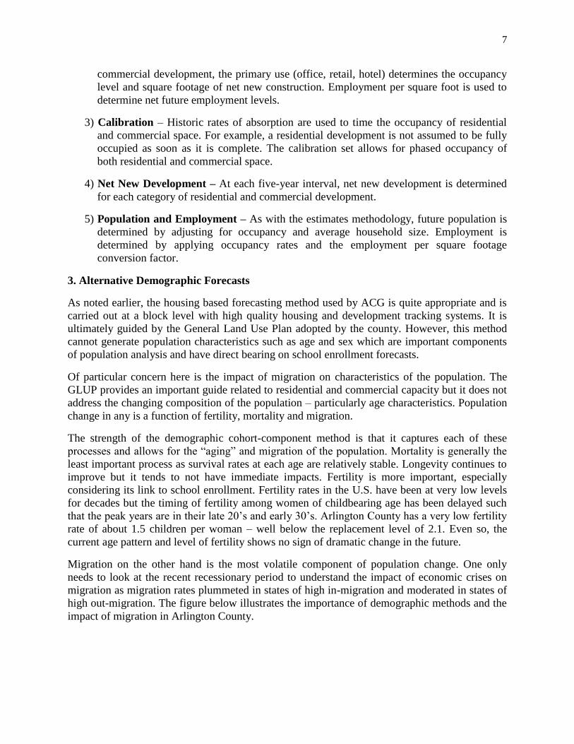
high out-migration. The figure below illustrates the importance of demographic methods and the

impact of migration in Arlington County.

8

This migration pattern by age shows that Arlington County clearly attracts population in the late

teens and early 20’s at a very high rate. It also shows that in-migration drops sharply in the 30’s

and continues at a slight negative level throughout the age distribution. A similar pattern is seen

in the 1990 to 2000 period. High in-migration of the young population is characteristic of many

urban areas attracting young workers. However, in many areas this population then moves out

when they start to form families and look for alternative housing arrangements.

There are generally two components to this phenomena: in college towns it’s the enrollment in

college that accounts for high rates of “in-migration” while in urban centers the migration is in

search of employment. College populations must be accounted for separately because they

distort the migration and fertility rates of the underlying population. College students are

“replaced” each year as one group graduates and a new group of freshmen enter therefore the

change in college population needs to be handled separately from the migration of the general

population.

Analysis of Arlington’s age distribution in 1990, 2000 and 2010 indicate that this young

population does not age in Arlington County and therefore is more likely to behave as a special

population indicative of a college town. In 1990 the 20 to 34 year old population was 31.6

percent of the total. In 2000 the same ages represented 33.9 percent and 36.2 percent in 2010.

The consistency of this age group and of the cohort ages 30 to 44 in each subsequent decade

support the notion that this migration bulge is related to the college population. The 2010 Census

shows that Arlington’s population living in group quarters (college housing) was only 610.

However, American Community Survey data reports the population living in Arlington and

enrolled in undergraduate and graduate colleges exceeds 20,000. Such a difference between the

college group quarters population and the college enrollment points to a need for better

understanding of migration and its age effects. This will have direct impacts on fertility forecasts

and school enrollment.

9

Recommendations

This review of the ACG estimates and forecasting methodology, along with the illustration of the

importance of demographic methods for a more complete understanding of the future housing

and population pressures leads to the following recommendations for immediate implementation

and additional study:

Immediate Implementation

1. Methods Documentation – ACG should consider development of comprehensive

methodology documentation. There are a variety of methods statements that have been

provided by ACG staff and on the website, but it is difficult to get a single, detailed

description of the methods employed. The county’s estimates and forecasting system is

quite detailed and staff have in-depth knowledge of the data sources and interaction.

Transparency of their data and methods would be improved by system documentation

that identifies the process, data sources, and assumptions.

2. Monitor ACS Housing Occupancy – Housing occupancy rates for each planning area

are based on the 2010 Census and are held constant throughout the estimates and forecast

periods. The census is the best benchmark for residential housing especially for small

geographic areas. However, economic conditions and development plans can alter

occupancy rates. ACG should continue to monitor the American Community Survey

results at the block group level but also use larger sample areas at the census tract and

county level to monitor housing occupancy. Margins of error in the ACS data can be

large for small areas but the data at the county and tract level can also point to trends that

can help inform changes at the planning area level.

3. Monitor ACS Average Household Size – As with housing occupancy, the ACG

methods rely on an assumption of a constant average household size for residential

development. Here again, the American Community Survey data at the tract and county

level should complement the use of block group data to identify trends that would inform

future assumptions about change in average household size.

Additional Study and Resources

4. Age Distribution Analysis – The age composition of the population is an important

driver of housing needs and development, yet this is an area that receives limited

attention in the estimates methodology and is not incorporated in the forecast process at

all. This initial review of migration by age indicates that more detailed analysis is

necessary to understand both the migration and aging effects in Arlington. Reliance on

the Census Bureau’s age estimates is a reasonable approach for developing current

estimates when close to the Census base. However, Arlington’s high proportion of

population in the 20 to 34 year age categories warrants detailed analysis of aging in the

county. This should include historical analysis of decennial census and current estimates

back to 1990 along with residual net-migration analysis to determine if this population

ages in the county or is a function of the high college enrolled population.

10

5. Migration Analysis Using Census Microdata – Analysis of the American Community

Survey Public Use Microdata Samples can identify migration flows (both in- and out-

migrants) and the demographic characteristics of migrants. Arlington County is defined

by two Public Use Microdata Areas and this would allow for some additional geographic

detail within the county. The ACG should acquire the necessary processing capability

and expand analysis of the microdata.

6. Development of Cohort-Component Demographic Forecasts – Analysis of aging and

the college population points to the need for adoption of a demographic cohort-

component method integrated with the existing housing based model. As noted earlier,

the demographic method has no explicit controls for housing capacity and the county’s

housing method is probably superior for forecasting total population. However, the

housing method cannot be used to generate age distributions and it can be seen from the

migration patterns that Arlington County’s population, and age composition, is greatly

influenced by migration.

7. Analysis of Self-Employment – Employment estimates and forecasts are driven by

office, retail and other commercial development as measured by square footage and a

conversion factor used to measure average square footage per employee. The data used

in the ACG method appears to adequately track current and future development.

However, establishment based employment does not do a good job of measuring the self-

employed, changes in multiple job holding and space sharing that is increasingly

common in office employment. ACG utilizes American Community Survey data on self-

employment to add the self-employed to the establishment employment base. Current

ACS data seems to only account for about 20 percent of the U.S. Bureau of Economic

Analysis proprietor’s employment of 29,000 in 2013 so additional analysis of the self-

employment component is warranted. ACG should evaluate the need to expand the

employment models to monitor and incorporate proprietor’s employment and the impact

of office space sharing in both public and private sector employment.

8. Integrated Economic/Demographic Modeling – While not a requirement of the

MWCOG Regional Cooperative Forecast process, the integration of an economic-

demographic model and the current housing/commercial space forecast should be

considered. Such integration can provide a “control” process that accounts for housing

and land development and constraints in the General Land Use Plan, employment growth

by economic sector, and implied population change. Employment, labor force, and

population change all impact commuting patterns which are also driven by workplace

employment. Currently, capacity in housing and commercial space are the controls but

there is no resulting analysis of those impacts on population by age and labor force

participation.

11

Arlington Public Schools

Enrollment Projection Methodology

APS uses the Grade Progression Ratio (“GPR”) method to project future enrollments. Also

known as the Cohort-Survival Ratio (“CSR”) method, GPR is the preferred method to project

enrollments by school demographers across the country. In essence, the method looks at

historical grade-to-grade progression ratios and assumes the historical progression ratios will

continue into the future, which essentially provides a linear projection of the population.

Typically, GPR is most effective when a district’s current trend continues into the future. In this

method, a ratio is computed for each grade progression, which essentially compares the number

of students in a particular grade to the number of students in the previous grade during the

previous year. The ratio indicates whether the enrollment is stable, increasing, or decreasing. A

grade progression ratio of one indicates stable enrollment, less than one indicates declining

enrollment, while greater than one indicates increasing enrollment. If, for example, a school

district had 100 fourth graders and the next year had 95 fifth graders, the survival ratio would be

0.95.

Researchers have debated the predictive ability of GPR; some claim it has a predictive validity

for one to two years, others believe it is valid for less than five years, while some state it can be

valid for as many as seven years. After one to two years, the projections can be inaccurate since

GPR’s major assumption is a linear trend, which may not hold true after a few years. GPR uses

three inputs to project enrollments: historical enrollments, live births, and new housing.

1. Historical Enrollment

To compute the progression ratios, APS uses the district’s September 30th

historical enrollment

counts. Since enrollment can vary in a district on a month-to-month basis, most districts report

their enrollment on the same day each year (e.g. October 15) to maintain a level of consistency.

In reviewing spreadsheets provided by the district, grade progression ratios were computed by

APS for the last fourteen years to show changes in the ratios over time. To project future

enrollments, APS uses an average of the last three grade progression ratios. While APS refers to

it as a 3-year average ratio, in actuality it is a 4-year ratio since it takes four historical years to

make three progression ratios. It is typical of school demographers to use a number of years in

computing progression ratios since it removes any one-time anomalies in the enrollment data that

may occur. The average progression ratios are applied to the most current enrollment to project

the next year’s enrollment. The process is repeated for the entire enrollment projection period,

which is usually five or ten years. APS projects enrollment for a ten-year timeframe. It should

be noted that a five-year projection is more reliable than a ten-year projection. If birth data are

used to project kindergarten students five years later, the ten-year projection in years 6-10 relies

on estimated birth counts (since the children have not yet been born) in order to project the

number of kindergarten students. For this reason, elementary projections are much more

susceptible to higher error rates in a ten-year projection as compared to middle or high school

projections, which rely on either children that have already been born or that are currently

enrolled in the district.

12

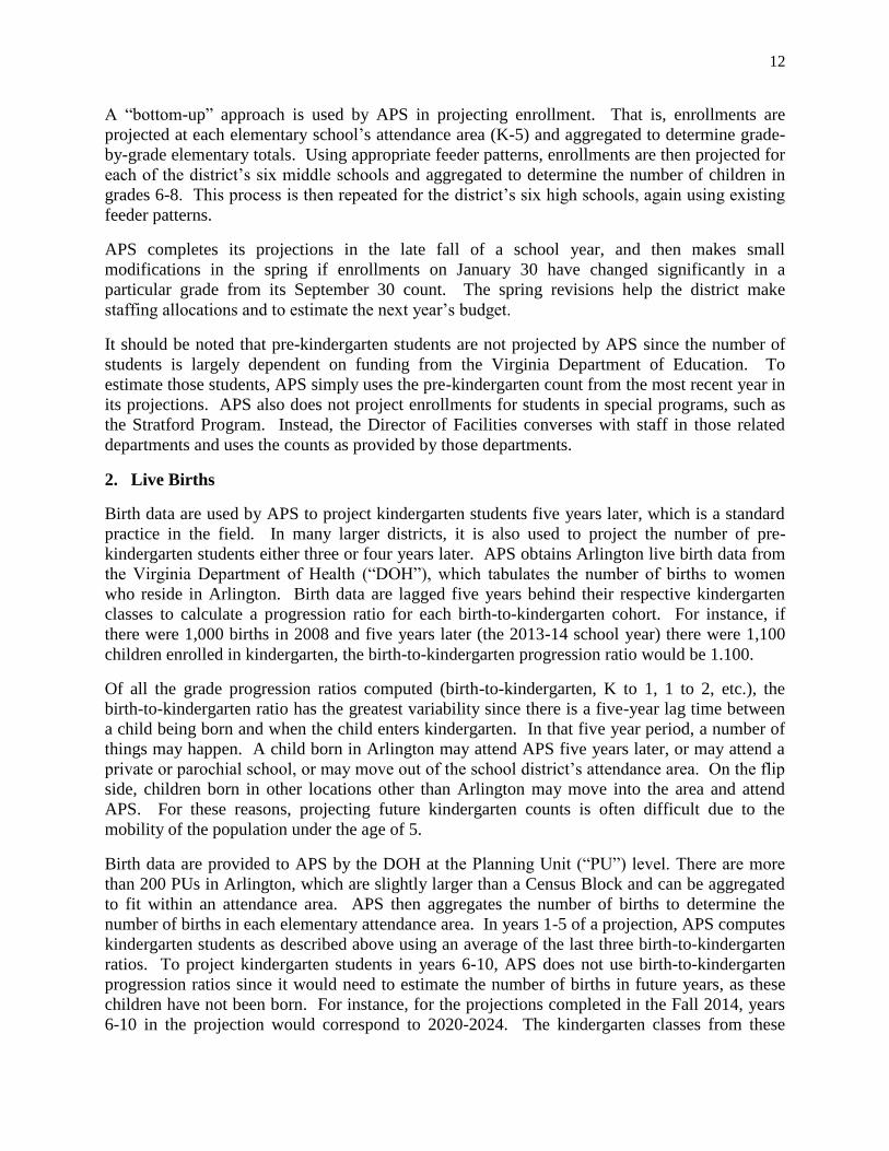
A “bottom-up” approach is used by APS in projecting enrollment. That is, enrollments are

projected at each elementary school’s attendance area (K-5) and aggregated to determine grade-

by-grade elementary totals. Using appropriate feeder patterns, enrollments are then projected for

each of the district’s six middle schools and aggregated to determine the number of children in

grades 6-8. This process is then repeated for the district’s six high schools, again using existing

feeder patterns.

APS completes its projections in the late fall of a school year, and then makes small

modifications in the spring if enrollments on January 30 have changed significantly in a

particular grade from its September 30 count. The spring revisions help the district make

staffing allocations and to estimate the next year’s budget.

It should be noted that pre-kindergarten students are not projected by APS since the number of

students is largely dependent on funding from the Virginia Department of Education. To

estimate those students, APS simply uses the pre-kindergarten count from the most recent year in

its projections. APS also does not project enrollments for students in special programs, such as

the Stratford Program. Instead, the Director of Facilities converses with staff in those related

departments and uses the counts as provided by those departments.

2. Live Births

Birth data are used by APS to project kindergarten students five years later, which is a standard

practice in the field. In many larger districts, it is also used to project the number of pre-

kindergarten students either three or four years later. APS obtains Arlington live birth data from

the Virginia Department of Health (“DOH”), which tabulates the number of births to women

who reside in Arlington. Birth data are lagged five years behind their respective kindergarten

classes to calculate a progression ratio for each birth-to-kindergarten cohort. For instance, if

there were 1,000 births in 2008 and five years later (the 2013-14 school year) there were 1,100

children enrolled in kindergarten, the birth-to-kindergarten progression ratio would be 1.100.

Of all the grade progression ratios computed (birth-to-kindergarten, K to 1, 1 to 2, etc.), the

birth-to-kindergarten ratio has the greatest variability since there is a five-year lag time between

a child being born and when the child enters kindergarten. In that five year period, a number of

things may happen. A child born in Arlington may attend APS five years later, or may attend a

private or parochial school, or may move out of the school district’s attendance area. On the flip

side, children born in other locations other than Arlington may move into the area and attend

APS. For these reasons, projecting future kindergarten counts is often difficult due to the

mobility of the population under the age of 5.

Birth data are provided to APS by the DOH at the Planning Unit (“PU”) level. There are more

than 200 PUs in Arlington, which are slightly larger than a Census Block and can be aggregated

to fit within an attendance area. APS then aggregates the number of births to determine the

number of births in each elementary attendance area. In years 1-5 of a projection, APS computes

kindergarten students as described above using an average of the last three birth-to-kindergarten

ratios. To project kindergarten students in years 6-10, APS does not use birth-to-kindergarten

progression ratios since it would need to estimate the number of births in future years, as these

children have not been born. For instance, for the projections completed in the Fall 2014, years

6-10 in the projection would correspond to 2020-2024. The kindergarten classes from these

13

years would have been born five years prior, which is 2015-2019. Since these years are in the

future, birth data would need to be estimated to project future kindergarten counts. Instead, APS

does a rolling average of the last three kindergarten classes to project future kindergarten counts.

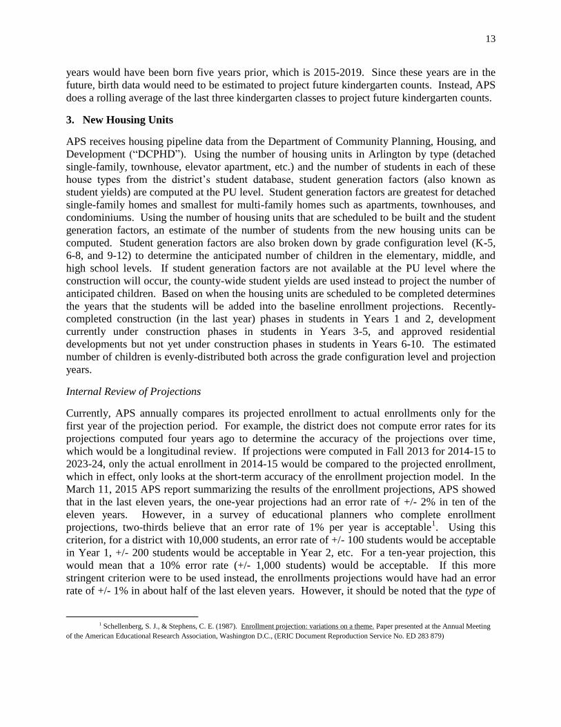
3. New Housing Units

APS receives housing pipeline data from the Department of Community Planning, Housing, and

Development (“DCPHD”). Using the number of housing units in Arlington by type (detached

single-family, townhouse, elevator apartment, etc.) and the number of students in each of these

house types from the district’s student database, student generation factors (also known as

student yields) are computed at the PU level. Student generation factors are greatest for detached

single-family homes and smallest for multi-family homes such as apartments, townhouses, and

condominiums. Using the number of housing units that are scheduled to be built and the student

generation factors, an estimate of the number of students from the new housing units can be

computed. Student generation factors are also broken down by grade configuration level (K-5,

6-8, and 9-12) to determine the anticipated number of children in the elementary, middle, and

high school levels. If student generation factors are not available at the PU level where the

construction will occur, the county-wide student yields are used instead to project the number of

anticipated children. Based on when the housing units are scheduled to be completed determines

the years that the students will be added into the baseline enrollment projections. Recently-

completed construction (in the last year) phases in students in Years 1 and 2, development

currently under construction phases in students in Years 3-5, and approved residential

developments but not yet under construction phases in students in Years 6-10. The estimated

number of children is evenly-distributed both across the grade configuration level and projection

years.

Internal Review of Projections

Currently, APS annually compares its projected enrollment to actual enrollments only for the

first year of the projection period. For example, the district does not compute error rates for its

projections computed four years ago to determine the accuracy of the projections over time,

which would be a longitudinal review. If projections were computed in Fall 2013 for 2014-15 to

2023-24, only the actual enrollment in 2014-15 would be compared to the projected enrollment,

which in effect, only looks at the short-term accuracy of the enrollment projection model. In the

March 11, 2015 APS report summarizing the results of the enrollment projections, APS showed

that in the last eleven years, the one-year projections had an error rate of +/- 2% in ten of the

eleven years. However, in a survey of educational planners who complete enrollment

projections, two-thirds believe that an error rate of 1% per year is acceptable1. Using this

criterion, for a district with 10,000 students, an error rate of +/- 100 students would be acceptable

in Year 1, +/- 200 students would be acceptable in Year 2, etc. For a ten-year projection, this

would mean that a 10% error rate (+/- 1,000 students) would be acceptable. If this more

stringent criterion were to be used instead, the enrollments projections would have had an error

rate of +/- 1% in about half of the last eleven years. However, it should be noted that the type of

1 Schellenberg, S. J., & Stephens, C. E. (1987). Enrollment projection: variations on a theme. Paper presented at the Annual Meeting

of the American Educational Research Association, Washington D.C., (ERIC Document Reproduction Service No. ED 283 879)

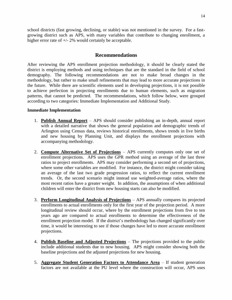
14

school districts (fast growing, declining, or stable) was not mentioned in the survey. For a fast-

growing district such as APS, with many variables that contribute to changing enrollment, a

higher error rate of +/- 2% would certainly be acceptable.

Recommendations

After reviewing the APS enrollment projection methodology, it should be clearly stated the

district is employing methods and using techniques that are the standard in the field of school

demography. The following recommendations are not to make broad changes in the

methodology, but rather to make small refinements that may lead to more accurate projections in

the future. While there are scientific elements used in developing projections, it is not possible

to achieve perfection in projecting enrollments due to human elements, such as migration

patterns, that cannot be predicted. The recommendations, which follow below, were grouped

according to two categories: Immediate Implementation and Additional Study.

Immediate Implementation

1. Publish Annual Report – APS should consider publishing an in-depth, annual report

with a detailed narrative that shows the general population and demographic trends of

Arlington using Census data, reviews historical enrollments, shows trends in live births

and new housing by Planning Unit, and displays the enrollment projections with

accompanying methodology.

2. Compute Alternative Set of Projections – APS currently computes only one set of

enrollment projections. APS uses the GPR method using an average of the last three

ratios to project enrollments. APS may consider performing a second set of projections,

where some other variables are modified. For instance, the district might consider taking

an average of the last two grade progression ratios, to reflect the current enrollment

trends. Or, the second scenario might instead use weighted-average ratios, where the

most recent ratios have a greater weight. In addition, the assumptions of when additional

children will enter the district from new housing starts can also be modified.

3. Perform Longitudinal Analysis of Projections – APS annually compares its projected

enrollments to actual enrollments only for the first year of the projection period. A more

longitudinal review should occur, where by the enrollment projections from five to ten

years ago are compared to actual enrollments to determine the effectiveness of the

enrollment projection model. If the district’s methodology has changed significantly over

time, it would be interesting to see if those changes have led to more accurate enrollment

projections.

4. Publish Baseline and Adjusted Projections – The projections provided to the public

include additional students due to new housing. APS might consider showing both the

baseline projections and the adjusted projections for new housing.

5. Aggregate Student Generation Factors to Attendance Area – If student generation

factors are not available at the PU level where the construction will occur, APS uses

15

county-wide student yields to project the number of anticipated children. Instead of using

county-wide yields, APS should consider aggregating the PU yields within an attendance

area and use those yields to project the future number of children. In this fashion, the

local information of the geographic area is not lost as it is currently when county-wide

yields are used.

6. Consider Past Home Construction Before Adding Students from New Home

Construction – Student generation factors from each PU level are currently being used

to project the number of students from new housing, and then are added to the baseline

projections based on the development timeline. It should be noted that the baseline

enrollment projections utilize grade progression ratios that do take into account prior new

home construction growth. Students who have moved into new housing and have

enrolled in the district have been captured by the progression ratios. Therefore, the total

number of children from future housing should not be added to the baseline projections in

order to avoid double-counting. Instead, the difference between the number of children

from future units and the number of children from recent historical construction in each

PU should be added to the baseline counts. For instance, if 500 detached single-family

homes were constructed in the last five years and generated an estimated 500 public

school children, the progression ratios would have captured these students entering the

district. If 700 detached single-family homes are planned in the next five years with an

estimated 700 children, only the difference, 200 children, should be added to the

projections since the ratios have already increased due to the children from new housing.

7. Update APS Website – Information describing the enrollment projection methodology

found on the APS website needs to be updated. For instance, the website states that

“Arlington uses the U.S. Census, reported in 10-year intervals, to conduct 10-year

projections and study historical trends.” APS currently does not integrate Census data

into the enrollment projections, which indicates that this is an outdated statement.

Additional Study and Resources

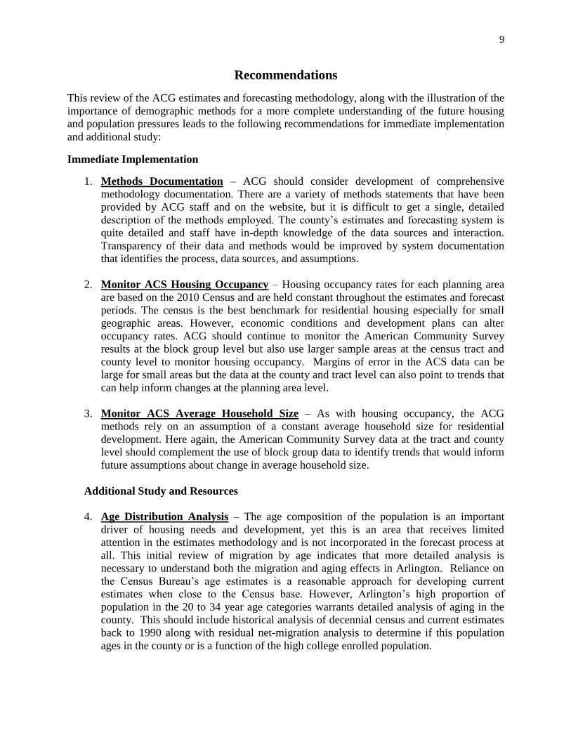
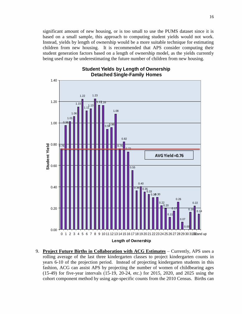
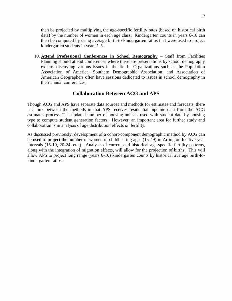
8. Compute Student Generation Factors by Length of Ownership – The student

generation factors (student yields) are computed by dividing the number of students in a

particular housing unit type (detached single-family, townhouse, etc.) by the number of

housing units of that type at the PU level. The generation factors therefore include homes

owned by all age segments of the population, which lowers the overall student yield. Dr.

Grip’s research has shown that student yields vary with lengths of ownership. An

example of student yields by length of ownership for detached single-family homes is

shown below for a community in New Jersey. Long-held homes (20 or more years) will

have fewer children, as they would have graduated from the district. Typically, yields

gradually increase with length of ownership, peaking at around 8-10 years of ownership.

Student yields at these lengths of ownership are higher than when considering average

yields for the entire population. Communities with excellent school districts often have

new homes that are purchased with greater frequency by families with children. In

computing student yields, some school districts use the Public Use Microdata Sample

(“PUMS”) from the Census Bureau to obtain the number of students in recently-

constructed homes in the last ten years. However, if a community has not had a

16

significant amount of new housing, or is too small to use the PUMS dataset since it is

based on a small sample, this approach to computing student yields would not work.

Instead, yields by length of ownership would be a more suitable technique for estimating

children from new housing. It is recommended that APS consider computing their

student generation factors based on a length of ownership model, as the yields currently

being used may be underestimating the future number of children from new housing.

0.76

0.98

1.01

1.06

1.15

1.22

1.111.13

1.23

1.171.16

0.940.96

1.08

0.76

0.82

0.73

0.55

0.36

0.40

0.350.33

0.300.30

0.220.20

0.11

0.17

0.26

0.07

0.00

0.16

0.22

0.14

0.00

0.20

0.40

0.60

0.80

1.00

1.20

1.40

0 1 2 3 4 5 6 7 8 9 10 11 12 13 14 15 16 17 18 19 20 21 22 23 24 25 26 27 28 29 30 31 3233 and up

Stu

de

nt

Yie

ld

Length of Ownership

Student Yields by Length of OwnershipDetached Single-Family Homes

AVG Yield =0.76

9. Project Future Births in Collaboration with ACG Estimates – Currently, APS uses a

rolling average of the last three kindergarten classes to project kindergarten counts in

years 6-10 of the projection period. Instead of projecting kindergarten students in this

fashion, ACG can assist APS by projecting the number of women of childbearing ages

(15-49) for five-year intervals (15-19, 20-24, etc.) for 2015, 2020, and 2025 using the

cohort component method by using age-specific counts from the 2010 Census. Births can

17

then be projected by multiplying the age-specific fertility rates (based on historical birth

data) by the number of women in each age class. Kindergarten counts in years 6-10 can

then be computed by using average birth-to-kindergarten ratios that were used to project

kindergarten students in years 1-5.

10. Attend Professional Conferences in School Demography – Staff from Facilities

Planning should attend conferences where there are presentations by school demography

experts discussing various issues in the field. Organizations such as the Population

Association of America, Southern Demographic Association, and Association of

American Geographers often have sessions dedicated to issues in school demography in

their annual conferences.

Collaboration Between ACG and APS

Though ACG and APS have separate data sources and methods for estimates and forecasts, there

is a link between the methods in that APS receives residential pipeline data from the ACG

estimates process. The updated number of housing units is used with student data by housing

type to compute student generation factors. However, an important area for further study and

collaboration is in analysis of age distribution effects on fertility.

As discussed previously, development of a cohort-component demographic method by ACG can

be used to project the number of women of childbearing ages (15-49) in Arlington for five-year

intervals (15-19, 20-24, etc.). Analysis of current and historical age-specific fertility patterns,

along with the integration of migration effects, will allow for the projection of births. This will

allow APS to project long range (years 6-10) kindergarten counts by historical average birth-to-

kindergarten ratios.