a review of the scale problem and applications of stochastic
TRANSCRIPT
_ _DANIEL B. STEPHENS & ASSOCIATES, INC.CONSULTANTS IN GROUND.WATER HYDROLOGY SOWOl
A REVIEW OF THE SCALE PROBLEMAPPLICATIONS OF STOCHASTIC MET
DETERMINE GROUNDWATERTRAVEL TIME AND PATH
RHO, NEW MEXICO
ANDHODS TO
BYT.-C. JIM YEH
AND
DANIEL B. STEPHENS
-
SUBMITTED TONUCLEAR WASTE CONSULTANTS
ANDU. S. NUCLEAR REGULATORY COMMISSION
SEPTEMBER 1988
- * GROUND-WATER CONTAMINATION * UNSATURATED ZONE INVESTIGATIONS * WATER SUPPLY DEVELOPMENT-

NUCLEAR WASTE CONSULTANTS INC.I 5s South Maid ison Street. SuitC 3(0
Den^1ver. C oloradko 80091'0-)14R130) 39-96957 FAX (30d) 39-)-9701
September 30, 1988 009/Tsk5/NWC.013RS-NMS-85-009Communication No. 287
U.S. Nuclear Regulatory CommissionDivision of High-Level Waste ManagementTechnical Review BranchOWFN - 4H3Washington, DC 20555
Attention: Mr. Jeff Pohle, Project OfficerTechnical Assistance in Hydrogeology - Project B (RS-NMS-85-009)
Re: Task 5 - A Review of the Scale Problem and Applications of StochasticMethods to Determine Groundwater Travel Time and Path, by T.-C. Jim Yehand Daniel B. Stephens
Dear Mr. Pohle:
Attached please find the final version of the Task 5 report, "A Review of theScale Problem and Applications of Stochastic Methods to Determine GroundwaterTravel Time and Path", by Drs. T.-C. Jim Yeh and Daniel B. Stephens (Daniel B.Stephens and Associates). The report, prepared under the QA program of DBS,has been reviewed by M. Logsdon of Nuclear Waste Consultants and received anexternal technical review from Dr. Alan Gutjahr of New Mexico Institute ofMining and Technology. For your information, I am enclosing a copy of Dr.Gutjahr's review comments.
The report addresses the following items:
o review of uncertainties in groundwater travel time and path that maybe attributed to hydrogeologic parameters;
o critical reviews of relevant scientific publications concerninguncertainties in travel time and path;
o discussion of the significance of the finding for the NRC's wastemanagement program;
o explanations and illustrations of stochastic concepts and methods ofstochastic analyses;
o presentation of a glossary of terms relevant to stochastic analyses.
009 - Tsk 5 - Yeh/Stephens -2 September 30, 1988
The final report has been reorganized and supplemented in the manner describedin NWC Communication No. 270, in which we transmitted the first draft of thereport. NWC considers that the revisions have made the entire work a muchbetter focused and more easily used report. In particular, the front materialsets the framework for the analysis that follows, new illustrations make theconcepts much more accessible, and the detailed mathematical derivations ofthe earlier version's Section 2 have been moved to an appendix. Thebibliography contains almost 400 citations to the literature on geostatisticaland stochastic methods in groundwater hydrology.
Most readers at the NRC, after looking at the abstract and the front material,will probably turn to Section 3, Groundwater Travel Times and Paths. Notethat there is material pertaining to groundwater travel time and pathsthroughout the text, not only in this section. After reviewing the text, NWCconsiders that you will find that Drs. Yeh and Stephens have reachedessentially the same conclusions that have been reached by the CNWRA ProgramArchitecture working group on GWTT: there are ambiguities in the wording ofthe current version of the performance objective (10 CFR 60.113 (a) (2)) thatneed further consideration. Yeh and Stephens propose a technical alternativeto the current form of the rule, based on the travel time of a certainconcentration of a hypothetical tracer released under pre-emplacementconditions. This technical alternative is not one that has been considered sofar by the CNWRA group, but it is conceptually similar to aspects of theanalysis originally prepared by Dr. Richard Codell of the NRC (Draft GenericPosition on Groundwater Travel Time, June 30, 1986). Yeh and Stephens presentthe arguments for why the transport analysis is a technically sound surrogatefor the performance of the natural system. It should be noted that theanalysis could still be relatively simple (at least compared to analyses forthe overall system performance), since the analysis would be performed underisothermal (or nearly so) conditions and could be limited to an ideallyconservative tracer to eliminate geochemical complications. This analysiswould allow consideration of such physical characteristics of the flow systemas the applicant could document are a functional part of the natural barrier,which is after all, what is to be shown. For example, if the applicant coulddemonstrate that dead-end pore spaces in a dual-porosity system were effectiveat isolating radionuclides under pre-emplacement conditions, then this wouldseem a legitimate part of the credit that they might wish to claim. Theirburden would be to demonstrate that the model they invoke and the data theyuse are reasonable for the site. This is no different as a matter of proofthan would be the burden to demonstrate a representative value for effectiveporosity in a one-dimensional seepage-velocity analysis. Reasonable technicalpeople could disagree with the Yeh/Stephens analysis, and there may well bepolicy reasons for which this approach would be found unsatisfactory. But NWCconsiders that Yeh and Stephens have presented their position clearly and thatit is one which should receive consideration.
Nuclear Waste Consultants, Inc.
009 - Tsk 5 - Yeh/Stephens -3 September 30, 1988
Transmittal of this report completes the deliverable for Task 5 under theAugust 14, 1987 direction of the NRC Project Officer. If you have anyquestions about this letter or about the report by Drs. Yeh and Stephens,please contact me immediately.
Respectfully submitted,NUCLEAR WASTE CONSULTANTS, INC.
Mark J. Logsdon, Project Manager
Att: A Review of the Scale Problem and Applications of Stochastic Methodsto Determine Groundwater Travel Time and Path, by T.-C. Jim Yeh and Daniel B.Stephens
cc: US NRC - Director, NMSS (ATTN PSB)HLWM (ATTN Division Director)Edna Knox, Contract Administrator (Documentation only)HLTR (ATTN Branch Chief)R. Codell, HLOBD. Chery, HLTR
CNWRA - Dr. John-Russell
L. Davis, WWL
bc: J. Minier, DBS
Nuclear Waste Consultants, Inc.

ACKNOWLEDGEMENTS
The authors wish to extend thanks to Dr. Allan L. Gutjahr at New MexicoInstitute of Mining and Technology for his constructive comments and suggestions.Many thanks go to Mr. Guzman Amado for his hard working and Mr. YoukuanZhang and the staff of Daniel B. Stephens and Associates, Inc. Finally, the authorswould like to thank Ms. Deborah E. Greenholtz for editing of the manuscript andMs. Corla Thies for drafting of figures.
_______ DANIEL B. STEPHENS & ASSOCIATES, INC.
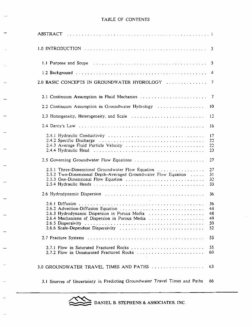
TABLE OF CONTENTS
ABSTRACT ........ . . . . . . . . . . . . . I
1.0 INTRODUCTION ..........................................
1.1 Purpose and Scope .......................................
1.2 Background .............................................
2.0 BASIC CONCEPTS IN GROUNDWATER HYDROLOGY ..............
3
3
4
7
2.1 Continuum Assumption in Fluid Mechanics ................
2.2 Continuum Assumption in Groundwater Hydrology ..........
2.3 Homogeneity, Heterogeneity, and Scale ...................
2.4 Darcy's Law .....................................
2.4.1 Hydraulic Conductivity ...........................2.4.2 Specific Discharge ..............................2.4.3 Average Fluid Particle Velocity .....................2.4.4 Hydraulic Head ................................
2.5 Governing Groundwater Flow Equations ..................
2.5.1 Three-Dimensional Groundwater Flow Equation ..........2.5.2 Two-Dimensional Depth-Averaged Groundwater Flow Equation2,5.3 One-Dimensional Flow Equation .....................2.5.4 Hydraulic Heads ................................
2.6 Hydrodynamic Dispersion ............................
2.6.1 Diffusion .....................................2.6.2 Advection-Diffusion Equation .......................2.6.3 Hydrodynamic Dispersion in Porous Media .............2.6.4 Mechanisms of Dispersion in Porous Media .............2.6.5 Dispersivity ...................................2.6.6 Scale-Dependent Dispersivity .......................
2.7 Fracture Systems ..................................
2.7.1 Flow in Saturated Fractured Rocks ...................2.7.2 Flow in Unsaturated Fractured Rocks .................
. . . 7
10
12
16
172 22323
27
27313233
36
364448495052
55
5560
63
66
3.0 GROUNDWATER TRAVEL TIMES AND PATHS ..................
3.1 Sources of Uncertainty in Predicting Groundwater Travel Times and Paths
DANIEL B. STEPHENS & ASSOCIATES, INC.

3.1.1 Uncertainty in Conceptualization . ... ....................3.1.2 Uncertainty in Mathematical Models ........................3.1.3 Uncertainty in Data Required by Mathematic Models ............
4.0 APPROACHES TO SPATIAL VARIABILITY .....................
4.1 Stochastic Representation of Hydrologic Properties .................
4.2 Geostatistics ...........................................
4.3 Stochastic Analysis of Spatial Variability ......................
6767i0
79
81
98
113
4.3.1 Monte Carlo Simulation ...4.3.2 Conditional Simulation ...4.3.3 Spectral Analysis .......4.3.4 Fractal Approach .......
.............................
.............................
.............................
114140149172
184
192
5.0: SUMMARY AND CONCLUSION ............................
REFERENCE ...............................................
APPENDIX A:
Glossary. Al
APPENDIX B:
Inconsistency in the Development of GoverningGroundwater Flow Equations .............................. BI
APPENDIX C:
Bibliography on Geostatistical and Stochastic MethodsRelated to Groundwater Hydrology .......................... Cl
. -_ - DANIEL B. STEPHENS & ASSOCIATES, INC.

LIST OF FIGURES
Figure 2.1. Dependence of velocity measurements uponsample size within a fluid ........ . . . . . . . . . . . . . . . . . . . . . . . . . 9
Figure 2.2. Different averaging volumes in fluid mechanics andporous media .1.1........ . . .. . .. . .. . . .. . .. . . .. . .. . . .. . . . I I
Figure 2.3. Effects of filters on noisy signals ...... . . . . . . . . . . . . . . . . . . 14
Figure 2.4. Effects of averaging volume on porosity distribution ..... . . . . . . 15
Figure 2.5. Hydraulic conductivity measurements using soil columns ..... . . . 19
Figure 2.6. Effect of velocity variations on outflow concentration ..... . . . . . 24
Figure 2.7. Concept of average hydraulic head distribution ..... . . . . . . . . . . 26
Figure 2.8. A control volume for mass balance ...... . . . . . . . . . . . . . . . . . 28
Figure 2.9. Water level in piezometers and a fully-screened well ..... . . . . . . 35
Figure 2.10. Smearing effect in a tank ....... . . . . . . . . . . . . . . . . . . . . . . . 37
Figure 2.11. A hypothetical velocity autocorrelation function ..... . . . . . . . . . . 42
Figure 2.12. A tracer experiment in a frictionless pipe ..... . . . . . . . . . . . . . . 45
Figure 2.13. Data showing the scale-dependent dispersivity ..... . . . . . . . . . . . 54
Figure 3.1. The actual and the predicted drawdown distributions ..... . . . . . . 74
Figure 4.1. Frequency distribution of the hydraulic conductivityof a sandy aquifer ........ . .. . . . . . . . .. . . . . . . . . . .. . . . . . . 83
Figure 4.2. Frequency distribution of the hydraulic conductivity ofa sandstone and a shale unit ....... . . . . . . . . . . . . . . . . . . . . . . . . 86
Figure 4.3. A schematic illustration of ensemble and realizationconcepts ........... .. . .. .. .. .. .. . .. .. .. .. . .. .. .. . .. . . 88
Figure 4.4. Diagrams to illustrate the concept of an autocorrelationfunction ........... .. .. . .. .. .. .. .. . .. .. .. . .. .. .. .. . . . 90
Figure 4.5. Schematic diagrams illustrating stochastic concepts ingroundwater hydrology ........ . . . . . . . . . . . . . . . . . . . . . . . . . . . 95
Figure 4.6. Some idealized time series and their autocorrelationfunctions...................................... ...... . 97
Figure 4.7. A cross-sectional view of the hydraulic conductivitydistribution in the Borden sandy aquifer ...... . . . . . . . . . . . . . . . . . 99
Figure 4.8. A cross-sectional view of the hydraulic conductivity
DANIEL B. STEPHENS & ASSOCIATES, INC.

distribution in the Borden sandy aquifer ...... . . . . . . . . . . . . . . . . 100
Figure 4.9. Vertical and horizontal autocorrelation functions forInK in the Borden sandy aquifer ....... . . . . . . . . . . . . . . . . . . . . 101
Figure 4.10. General behavior of a variogram ....... . . . . . . . . . . . . . . . . . 104
Figure 4.11. A diagram showing the shapes and equations of variousvariograms ........ . .. . . . . .. . . . . . . .. . . . . . . .. . . . . . . .. . 105
Figure 4.12. A variogram showing the nugget effect ...... . . . . . . . . . . . . . . 107
Figure 4.13. Hypothetical InK variogram illustrating the nestedcorrelation scale ........... .. . .. .. .. .. . .. .. .. .. . .. .. .. . 108
Figure 4.14. A schematic illustration of Monte Carlo simulationconcept .1.............. ... ... .. ... ... ... ... ... ... .. . . I15
Figure 4.15. Simulated hydraulic head distributions in heterogeneousaquifers .............. .. ... ... ... .. ... .. . 122
Figure 4.16. The ensemble averaged head distribution and its standarddeviation in a hypothetical aquifer .1.2.3.... . . . . . . . . . . . . . . . . . . 1 3
Figure 4.17. Cumulative probability distribution of simulatedgroundwater travel times ......... . . . . .. . . . . . .. . . . . . .. . . . . 125
Figure 4.18. Effects of finite difference block size on the probabilitydistribution of groundwater travel time ...... . . . . . . . . . . . . . . . . . 127
Figure 4.19. Effects of correlation scale of transmissivity onthe probability distribution of groundwater travel time ..... . . . . . . . 129
Figure 4.20. A comparison of the unfiltered and filtered log K dataalong a cross-section of a hypothetic aquifer ...... . . . . . . . . . . . . . 132
Figure 4.21. Particle arrival versus time curves ...... . . . . . . . . . . . . . . . . . 133
Figure 4.22. A schematic diagram of the layered geologic media witha thin high permeable layer ....... . . . . . . . . . . . . . . . . . . . . . . . 137
Figure 4.23. A schematic illustration of the conditional simulation ..... . . . . . 141
Figure 4.24. A prism acts as a frequency analyzer ...... . . . . . . . . . . . . . . 152
Figure 4.25. Anisotropy of effective hydraulic conductivity ..... . . . . . . . . . . 160
Figure 4.26. An observed depth-averaged and mean concetration profile .... . . 166
Figure 4.27. A comparison of observed and theoretical spatialconcentration variance ......... . . .. . . .. . . . .. . . . .. . . . .. . . 170
Figure 4.28. Schematic illustration of fractal concept ............ . .... .. 175
Figure 4.29. Schematic illustration of a linear relationship betweenfractal parameters. . . 176
-______ DANIEL B. STEPHENS & ASSOCIATES, INC.

LIST OF TABLES
Table 1. Variances and correlation scales ofr log hydraulic codnuctivityor log transmissivity .......... .. . .. . .. . .. . . .. . .. . .. . .. . . 93
Table 2.. Comparison of transport behavior in systems with thin highpermeable layer ........... .. . .. .. .. . .. .. . .. .. . .. .. . .. . I138
Table 3. Ratio of the coefficients of variation in various arrival timesresulting from the conditional simulation to those from theunconditional simulation ......... . . . . . . .. . . . . . . . .. . . . . . . 147
DANIEL B. STEPHENS & ASSOCIATES, INC.

Scale Problem and Stochastic Methods IPagte IScale Problem and Stochastic Methods Pat~~~~~~~~~~~e I
ABSTRACT
The groundwater travel time along the fastest path of likely radionuclide
transport is a regulatory criterion used to assess the hydrogeologic quality of a high-
level radioactive waste repository. Hydrologists and engineers are limited in their
ability to define with confidence the fastest path, owing to the heterogeneous nature
of geologic materials. Field measurements of hydraulic properties such as in test or
observation wells, are inherently averages of properties at scales smaller than the
scale of the field measurement. As a result of averaging, subscale information is lost
and there is uncertainty in defining the fastest trajectory of groundwater. This scale
problem is explained through a review of the continuum and REV concepts in
groundwater hydrology. The application of hydrodynamic dispersion concepts is
recommended as a means of incorporating the effect of subscale heterogeneity on the
fastest groundwater travel time.
Sources of uncertainties in predicting groundwater travel time are discussed
in the report. The uncertainties are mainly attributed to the heterogeneous nature of
geologic formations. The heterogeneity of geologic materials can, however, be
characterized quantitatively using geostatistical methods. Important statistical
parameters include mean and variance, as well as the spatial correlation structures of
the hydrologic properties within the hydrogeologic system. These parameters may be
obtained from limited data base. Stochastic methods, reviewed and explained in this
report, can take advantage of the geostatistical characterization to predict large-scale
groundwater flow and solute transport. Several examples from recent scientific
literature are provided to illustrate the application of stochastic methods to the
groundwater travel time analysis.
Stochastic methods in subsurface hydrology have only recently been
evaluated under field conditions for a few locations, and validation of the theories is
DANIEL B. STEPHENS & ASSOCIATES, INC.
Scale Problem and Stochastic Methods Page 2
incomplete, especially in unsaturated fractured rocks. Nevertheless, research efforts
should continue to improve the state-of-the art. Geostatistics and stochastic methods
will be valuable tools in addressing the groundwater travel time objective.
________ DANIEL B. STEPHENS & ASSOCIATES, INC.
Scale Problem and Stochastic Methods Page 3
1.0 INTRODUCTION
1.1 Purpose and Scope
Daniel B. Stephens & Associates, Inc. was requested by the U.S. Nuclear
Regulatory Commission (NRC), through Nuclear Waste Consultants, to conduct a
review of the literature pertaining to stochastic approaches for characterizing the
uncertainty in predicting groundwater travel path and travel time in saturated media.
Enclosed is the draft final report of this study. As directed by the NRC, the report
addresses the following:
-review of uncertainties in groundwater travel time and path which are
attributed to hydrogeologic parameters
-critical reviews of relevant scientific articles relevant to the analysis of
uncertainties in prediction of groundwater travel time and path
-a discussion of the significance of the findings to the NRC's waste
management program
-explanations and illustrations of the stochastic concept and methods of
stochastic analysis
-a glossary of terms relevant to stochastic analyses
In addition, the report discusses the concept of the representative elementary
volume (REV). The report also attempts to clarify the relationships between the
REV scale, the measurement scale of hydraulic properties and scale of modeling.
The proposed work is motivated in large part by federal regulations
pertaining to the performance of high level waste repositories, in particular, the
groundwater travel time (GWTT) objective. As stated in 10 CFR 60. 113(a)(2), the
GWTT performance objective is:
"The geologic repository shall be located so that pre-waste-
emplacement groundwater travel time along the fastest path of likely
DANIEL B. STEPHENS & ASSOCIATES, INC.

Scale Problem and Stochastic Methods l'atze
radionuclide travel from the disturbed zone to the accessible environment shall
be at least 1,000 years or such other time as may be approved or specified by
the Commission."
The NRC has drafted generic technical positions on groundwater travel time
to help explain this phase, as well as the rest of the regulation (NRC, 1986. 1988).
One of the key points requiring clarification is the definition of "the fastest path of
likely radionuclide transport". Hydrogeologists are well aware that there are many
possible pathways, but which one is the fastest and how fast does groundwater travel
along it? Herein. enters the element of uncertainty. There is uncertainty not only in
identifying the fastest path from limited subsurface data but also in travel time
owing to the uncertainty in path length as well as in data or approaches used to
compute travel time.
As our report will illustrate, stochastic methods are well-suited to deal wvith
uncertainty in groundwater travel time and travel path analysis. However, they have
only been developed for groundwater problems within the last decade. The
mathematical complexities presented in theoretical articles in the scientific literature
are not easily assimilated by most practitioners. Moreover, because field tests to
validate stochastic models have not been completed, most hydrogeologists are still
reluctant to apply these models. One of the underlying purposes of our review is to
explain the principles of stochastic models without resorting to the mathematical
details and give examples of how the stochastic methods may be applied in the
analysis of groundwater travel time and travel path.
1.2 Background
Uncertainties in predicting groundwater travel times and paths arise
primarily from heterogeneity of aquifer materials. Heterogeneity is a continuous
phenomenon: it exists at all scales (from microscale to megascale). However,
heterogeneous materials may be treated as homogeneous at one observation scale, and
DANIEL B. STEPHENS & ASSOCIATES, INC.

Scale Problem and Stochastic Methods Page 3
heterogeneous at a different scale. That is. the definition of heterogeneity is a relative
one, depending on the scale of observation. Thus, the heterogeneity observed is
directly related to the scale of the problem.
The problem of scale does not exist only in hydrology (Dooge, 1986). but
poses many difficulties for every branch of science and every one of us living in the
universe. It controls our perception of everything that we see and feel. The scale
problem is best illustrated in the book entitled "Powers of Ten" by Morrison and
Morrison (1982). The book contains visual images ranging from a scale of 1025
meters to 10-14 meters. At a scale of 1025 meters galaxies are seen as tiny clusters
in empty space. At a scale of 1023 meters, the Milky Way appears as one of a
number of bright spots in empty space. The spiral structure of the Milky Way
becomes apparent at a scale of 1021 meters. A scale of 1013 meters encompasses the
orbits and all the planets of the solar system. At the scale between 10-7 and l0-9
meters, we see the various structures of DNA molecules, and so on. Similarly, in
groundwater hydrology, at a scale of 106 meters one may observe variations among
groundwater basins. Various geologic formations become noticeable at a scale of 103
meters. A scale of 10 meters may encompass various layers of clay, sand, and
gravel. We can no longer recognize the irregularity of layers, but we do recognize
pore structures at a scale of 10-6 meters. Water molecules within pores are visible
at a scale of 10-8 meters. and so on as the scale of observation decreases.
Heterogeneity exists in groundwater hydrology at all scales. However. once
we select a scale of observation, we often neglect phenomena at subscales. This is
exactly the way our formulas, equations, and laws are developed in all sciences,
including groundwater hydrology. Subscale phenomena we ignored, however, may
play vital roles in solving or studying the problems of interest. Furthermore,
different laws and equations may be developed or discovered at different scales and
may not be appropriate for studying problems at another scale. For instance, a
DANIEL B. STEPHENS & ASSOCIATES, INC.

Scale Problem and Stochastic Methods Pag e 6
representative elementary volume as used in the study of flower through porous m1edlia
would be different from that for flow through fractures or karsts. When predicting
groundwater travel times and paths, we may face the difficulty of extrapolating
equations and laws developed for a small scale to solve problems at a larger scale,
for example over distances of 10 km or more.
In the following chapters, we will first discuss of the continuum hypothesis
in fluid mechanics and groundwater hydrology, and then we will show the
development of equations for groundwater flow at different scales. We will then
discuss the uncertainties in predicting groundwater travel times and paths and finally
review some recent advances in groundwater hydrology to tackle the scale related
problems.
DANIEL B. STEPHENS & ASSOCIATES, INC.

Scale Problem and Stochastic Methods Pagze 7
2.0 BASIC CONCEPTS IN GROUNDWATER HYDROLOGY
2.1 Continuum Assumption in Fluid Mechanics
The most fundamental assumption in fluid mechanics is the continuum
assumption in which the fluid is assumed to behave as if it were continuous in space
at the macroscopic scale, say 10-2 meters.
For example, at the macroscopic scale, one can see water in a garden hose.
and the water is continuous throughout the hose. However, if we examine a fluid at
the microscopic scale, say 10-8 meters, the mass of the material in a fluid is
concentrated in the nuclei of the atoms composing a molecule and is not uniformly
distributed over the column occupied by the liquid. Using the garden hose example,
we can view the velocity of water moving through the hose in perhaps two ways,
depending upon the scale of interest. In the first case, at the macroscopic scale, the
velocity is simply the volumetric discharge rate per unit cross-sectional area. For
steady-state conditions, the velocity is constant in space along the hose. In the
second case, at the microscopic scale, the velocity of individual fluid molecules is
highly variable along their path through the hose. This molecular velocity is
virtually impossible to measure. However. we are normally concerned with the
behavior of matter on a macroscopic scale which is much larger than the distance
between molecules. Accordingly, the properties of a fluid defined in fluid mechanics
have to represent the property values over such a macroscopic volume. The
properties contained in this volume are thus regarded as the average values being
spread uniformly over that volume instead of, as at the microscopic scale, being
concentrated in a small fraction of it. This macroscopic representation of the fluid
makes it possible to treat the fluid as a continuum in space. This approach in fluid
mechanics is known as the continuum approach and the associated hypothesis that the
DANIEL B. STEPHENS & ASSOCIATES, INC.

Scale Problem and Stochastic Methods Pagie S
fluid can be so represented is called the continuum approach.
Indeed. the properties of the fluid at the macroscopic scale are continuous
and smoothly varying, if observed with any of the conventional measuring devices.
When a measuring device is inserted in a fluid, it responds in some way to a
property of the fluid within some small neighboring volume, and provides a measure
which is effectively an average of that property over the volume. The device, such
as a pitometer for measuring velocity, is normally chosen so that the volume is small
enough for the measurement to be a local one; that is, further reduction of the
volume does not change the reading of the device. However, the volume is large
enough to contain an enormous number of molecules so that the fluctuations arising
from the different properties of molecules have no effect on the observed average.
Therefore, we can define a reproducible property of the fluid. Of course, if the
averaging volume is so small as to contain only a few molecules, the number and
kind of molecules in the volume at the instant of observation will fluctuate from one
observation to another, and the measurement will vary in an irregular way, with the
size of the averaging volume corresponding to the measuring device. Figure 2.1
illustrates the way in which a measurement of velocity of the fluid would depend on
the averaging volume of the device. We are able to regard the fluid as a continuum
when, as shown in the figure, the measured fluid property is constant for volumes
which are small on the macroscopic scale but large on the microscopic scale.
The continuum assumption allows us to attach a precise meaning to the
various physical properties at any point in space. The various fluid properties such
as density, velocity, and temperature can thus be treated as continuous functions of
time and position in the fluid which satisfy the requirements of differential calculus.
On this basis, we shall be able to establish differential equations governing the
motion of the fluid. The equations are macroscopic equations that are independent
of the nature of the particle structure which is generally discontinuous in space and
DANIEL B. STEPHENS & ASSOCIATES, INC.

Scale Problem and Stochastic Methods
C-)
-JLIJ
Pacpe Q
COrISTAilT VELOCITY
SAMPLE SIZE
Figure 2.1. Dependence of velocity measurements upon sample sizewithin a fluid.
DANIEL B. STEPHENS & ASSOCIATES, INC.

Scale Problem and Stochastic Methods Pace 10
time.
2.2 Continuum Assumption in Groundwater Hydrology
In saturated porous media (granular materials), flow takes p)lace throwu h a
complex network of interconnected pores or openings. Although the fluid itself may
be considered as a continuum by the continuum hypothesis used in fluid mechanics.
the flow path may be discontinuous because of the complex nature of the pore
geometry. Obviously, it is practically impossible to describe in any exact
mathematical manner the intricate pore structure which controls the flow through
porous media. As a result, one has to abandon the basic equations governing fluid
flow (such as the Navier-Stokes equations) at the pore-scale level. Similar to the
continuum hypothesis in fluid mechanics, groundwater hydrologists have to overlook
the microscopic or pore-scale flow patterns inside individual pores and consider some
average flow over a certain volume of porous media. By doing so. they are
employing the concept of a continuum, which is analogous to the concept used in
fluid mechanics and other branches of sciences. The minimum volume over which
the continuum assumption applies in flow through porous media, however, is much
larger than the one defined in fluid mechanics (Figure 2.2). In groundwater
hydrology, this volume is called the representative elementary volume (REV) (Bear,
1979). Using the REV concept. we essentially bypass both the microscopic level, at
which we consider what happens to each molecule in the fluid, and the pore level at
which we consider the flow pattern within each pore and between pores, and then
move to the macroscopic level at which only averaged phenomena over the REV are
considered. Thus. a REV is simply a volume over which we carry out the
averaging process. as shown in Figure 2.2.
A more practical definition of the REV may be given as follows: an REV is
a volume that is sufficiently large to contain a great number of pores so that a mean
property exists, and it is sufficiently small so that the parameter variations at a scale
._______ DANIEL B. STEPHENS & ASSOCIATES, INC.

Scale Problem and Stochastic Methods i.mae I I. .
REV for K * J Cporous i f I -
m edia _ _ _ _ _ _ _ _
REV for continuum fluid mechanics
Figure 2.2. Different averaging volumes in fluid mechanics andporous media.
DANIEL B. STEPHENS & ASSOCIATES, INC.

Scale Problem and Stochastic Methods l'a2e l'
larger than the size of REV can be represented by continuous functions which salisty
the requirements of the classic differential calculus (De Miarsily. 19S6).
The REV concept is also defined through a rigorous mathematical expression
suggested by Marie (1967). At pore-scale, the spatial distribution of pore openlings
could be highly erratic, analogous to electronic signals superimposed with random
noises. Then, an REV is merely a noise filter similar to the one in electrical
engineering that filters out the random noises and produces a smooth signal (Figure
2.3). Mathematically, this process can be formulated as:
H(x) = f h(x + i)) f(I) dj (22.11
where H(x) is the smoothed, continuous, output signal, h(x) is the original, noisy, and
erratic signal, and f(n1 ) is the filter or a weighting factor. Figure 2.3a shows a filter
function which eliminates high frequency noises but retains the smooth sinusoidal
signal. Some filter functions can smooth noises and signal as shown in Figure 2.3b.
In groundwater hydrology, H(x) is the macroscopic property of porous media and f(e)
is the weighting function used within the volume or window over which the pore-
scale properties are averaged, i.e., the REV. For example,
within the volume V
f () = (2.2.2)
t, otherwise
2.3 Homogeneity. Heterogeneity, and Scale
The definitions of homogeneity and heterogeneity follow from the concept of
the REV. From the previous discussion, it should be clear that as the size of the
_____ DANIEL B. STEPHENS & ASSOCIATES, INC.

Scale Problem and Stochastic Methods l'au e 13
window or the volume over which the averaging takes place increases, the noise level
in the output will decrease (Figures 2.3). Therefore, if one properly chooses the size
of the averaging volume, a material with a spatially-varying property may thus be
treated as a material with a spatially-constant property. This material is then
defined as homogeneous. This situation is analogous to that in Figure 2.3b. Now,
consider a porosity distribution of a hypothetical porous medium. If one chooses a
pin point as the sample size to define porosity, let us assume that Figure 2.4a would
represent the porosity distribution along a transect of the porous medium. At a
point, the void has a porosity value one, and the solid zero. If one averages the
values of porosity over a window that is larger than a point, say, as large as one
solid or void space, the "new" porosity distribution of the aquifer will look like that
shown in Figure 2.4b where the sharp boundary between voids and solid is smeared
out due to the averaging over the window. It should be evident that if a window
slightly larger than one solid space is used, the porosity values of the aquifer will
still vary in space but the variation will be relatively smooth and continuous.
Therefore, the aquifer is heterogeneous and it can be described by our continuum
mathematics. If one chooses a window which is equal to two void spaces to define
the porosity values at every point within the medium, the medium should obviously
have a constant porosity over the entire medium. In fact, the porosity will be 0.5
everywhere if the averaging window is equal to two void or solid spaces. Hence,
the medium as far as porosity is concerned is a homogeneous medium (Figure 2.4c).
This window can be considered as the minimum size of the REV for conceptualizing
the medium as a homogeneous one. Suppose one applies this window to another
porous medium which has a checkerboard porosity distribution but with larger void
and solid sizes. The porosity distribution defined by the average porosity over the
same window becomes nonuniform. In other words, the medium now is considered
heterogeneous. But, if one again chooses a window that is equal to the size of the
DANIEL B. STEPHENS & ASSOCIATES, INC.

Scale Problem and Stochastic Methods Page 14
(a)
INPUT SIGNAL OUTPUT SIGNALh(x) H(x)
(b)
INPUT SIGNAL OUTPUT SIGNALh(x) H(x)
Figure 2.3. Effects of filters on noisy signals.
a) Filter affects noise only, and b) filteraffects noise and most of signal.
DANIEL B. STEPHENS & ASSOCIATES, INC.

Scale Problem and Stochastic Methods P-1m I r s
Scale Prbe an Stcasi Mehd Pi * 1I -
SOL]
I'1.0
(a) C 0.5-
0
I v~~~~~~~~~~~~~~~~~~~~~~~~~~~~~
t~~~~~~~~~~~~~~~~~~~~~~~~~~~~~~
VOID
7 7-
x: v,, ,~~ ~~~~~~~~~~~~~~~~~~~~~~~~~.. S 6 S - 6 L
(b) 'C~
C)
x
1.0 t
(C) Ln °. 5CL
CONSTANT POROSITY, 0.5
I I . . . . . I . I
n _U . .
Figure 2.4. Effects of averaging volume on porosity distribution.(a) A hypothetical solid and void distribution. (b) Size ofaveraging volume equals one void volume. (c) Size of averagingvolume equals two void volumes.
DANIEL B. STEPHENS & ASSOCIATES, INC.

Scale Problem and Stochastic Methods l'.ce 16
two void or solid spaces of this checkerboard. one can define this mediumn as a
homogeneous porous medium. From this simple example. it can be seen that in mrder
to obtain the homogeneity, the size or the REV has to be much larger than the size
of heterogeneity.
The size of the REV varies with the size of the blocks in the examples or
the size of heterogeneity in reality. The size of heterogeneity depends on the scale
of the problem that we encounter. For instance, the heterogeneity within core
samples is likely due to the variation in grain size. We may call this variability the
laboratory-scale heterogeneity. Heterogeneity due to geologic stratification or lax ering
in a formation may be classified as the field-scale heterogeneity. The regionial-scale
heterogeneity then represents the variation of geologic formations or facies.
Furthermore, variations among sedimentary basins may be classified as the -lobal-
scale heterogeneity, and so on. Similar definitions of the scale of heterogeneity \w.ere
given by Dagan (1986) and Gelhar (1986). Regardless of the definition of the scale
of heterogeneity, one has to recognize that the heterogeneity is a continuous
phenomenon which exists at all scales.
2.4 Darcy's Law
With the concept of the REV in mind, one should recognize that every
property defined in groundwater hydrology (such as volumetric flow rate, hydraulic
head, porosity, hydraulic conductivity, and storativity, etc.) involves measurement over
a certain volume. The same is true for the principles and laws used in groundwater
hydrology. The most important example would be Darcy's law, which states that
groundwater specific discharge is linearly proportional to the hydraulic gradient with
a constant of proportionality:
q Q KI (2.4.1)
DANIEL B. STEPHENS & ASSOCIATES, INC.

Scale Problem and Stochastic Methods Page 17
where q is the specific discharge with dimensions of (LT-1). Q is the volumetric flowv
rate (L3T-1 ). I is the gradient (LL-1). A is the cross-sectional area perpendicular to
the direction of flow (L2), and K is a constant of proportionality which is usually
called hydraulic conductivity (LT-1). Darcy's law is an empirical equation. although
one can prove the validity of the equation using rigorous mathematics and physics
L (Hubbert. 1940). Nevertheless, it is simply a linear regression equation showing the
relationship between gradient and specific discharge through a column of soil of a
certain volume. Therefore. Darcy's law is a macroscopic law because the volume
L where the law applies is obviously much larger than many pores.
2.4.1 Hydraulic conductivity. In the laboratory, hydraulic conductivity is
L generally determined from a column test which uses either a constant head
permeameter or a falling head permeameter. Regardless of whether one uses a
L constant or falling head permeameter. the measured hydraulic conductivity is an
average value over the length of the column. To illustrate this point. we will
examine the case where the column consists of a single homogeneous soil. If a
L constant head permeameter is used, then steady-state flow will be established. The
flow rate through the column is, according to Darcy's law:
L
L Q - KAI - KA X Lh2 (2.4.2)
L where hi and h2 are the hydraulic heads measured at points I and 2, and L is the
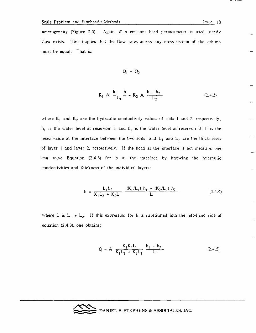
distance between the two points (Figure 2.5). If we measure Q. A, and 1. we
certainly can determine the K value, the hydraulic conductivity. Obviously. in a core
L sample, the calculated hydraulic conductivity. K. represents some average small-scale
hydraulic conductivity variations within the core. To illustrate the concept of an
L average K, we consider a second case where the porous medium contains layered
j ~ DANIEL B. STEPHENS & ASSOCIATES, INC.
Scale Problem and Stochastic Methods Plas e 1I
heterogeneity (Figure 2.5). Again, if a constant head permeameter is used. steldv
flow exists. This implies that the flow rates across any cross-section of the columnn
must be equal. That is:
QI = Q2
KI A Ih - K2 A h -h 2 (2.4.3)
where K, and K2 are the hydraulic conductivity values of soils I and 2, respectively;
h, is the water level at reservoir 1, and h, is the water level at reservoir 2; h is the
head value at the interface between the two soils; and L, and L2 are the thicknesses
of layer I and layer 2. respectively. If the head at the interface is not measure, one
can solve Equation (2.4.3) for h at the interface by knowing the hydraulic
conductivities and thickness of the individual layers:
LI L2
h = KIL 2 + K2L1(Kt/Lt) hi + (K2 /L2 ) h2
L(2.4.4)
where L is LI + L2. If this expression for h is substituted into the left-hand side of
equation (2.4.3), one obtains:
Q - A KIK 2 L hi - h2Q= A KIL 2 +K 2LI L (2.4.5)
DANIEL B. STEPHENS & ASSOCIATES, INC.

Scale Problem and Stochastic Methods Pia0e 19I,
CASE 1 CASE 2
Q Q
Q
DATUM
Figure 2.5. Hydraulic conductivity measurements using soil columns.Case 1 is a homogeneous(or equivalent homogeneous) soilcolumn, and Case 2 is a two layer soil column.
DANIEL B. STEPHENS & ASSOCIATES, INC.
Scale Problem and Stochastic Methods Pace 20
This is the formula to determine the flow rate through the core sample fronm the
permeameter. Let us attempt to determine the average hydraulic conductivity of this
two-layer soil column. If a constant head permeameter is used. Bee can measure
heads at the two ends of the column and the discharge from the column. Using the
measured heads and discharge rate. from Darcy's law (2.4.2), the hydraulic
conductivity can be easily determined by:
Kave - Q (2. 4.6)A(hl - h,)
When equation (2.4.6) is used, we evidently assume that there is an equivalent
homogeneous soil which should transmit the same amount of discharge as the layered
soil column under the same head drop. Therefore, the Kave value obtained from this
calculation represents the K value of the equivalent homogeneous soil column and
ignores the K values of each layer.
So, how is the Kave value related to the K values of each individual soil?
From a comparison of equation (2.4.2) and (2.4.5), one can see that:
Kat.e = L1I/K1 + L2 /K2
As indicated in equation (2.4.7), the K value of the equivalent homogeneous soil
column is the harmonic mean of the K's of individual soil layers. A similar analysis
can be done where flow is parallel to the layers in the soil column. In this case, the
average K obtained from the soil column will correspond to the arithmetic mean of
the K's of the individual layers. That is:
_______DANIEL B. STEPHENS & ASSOCIATES, INC.
Scale Problem and Stochastic Methods leasze 21
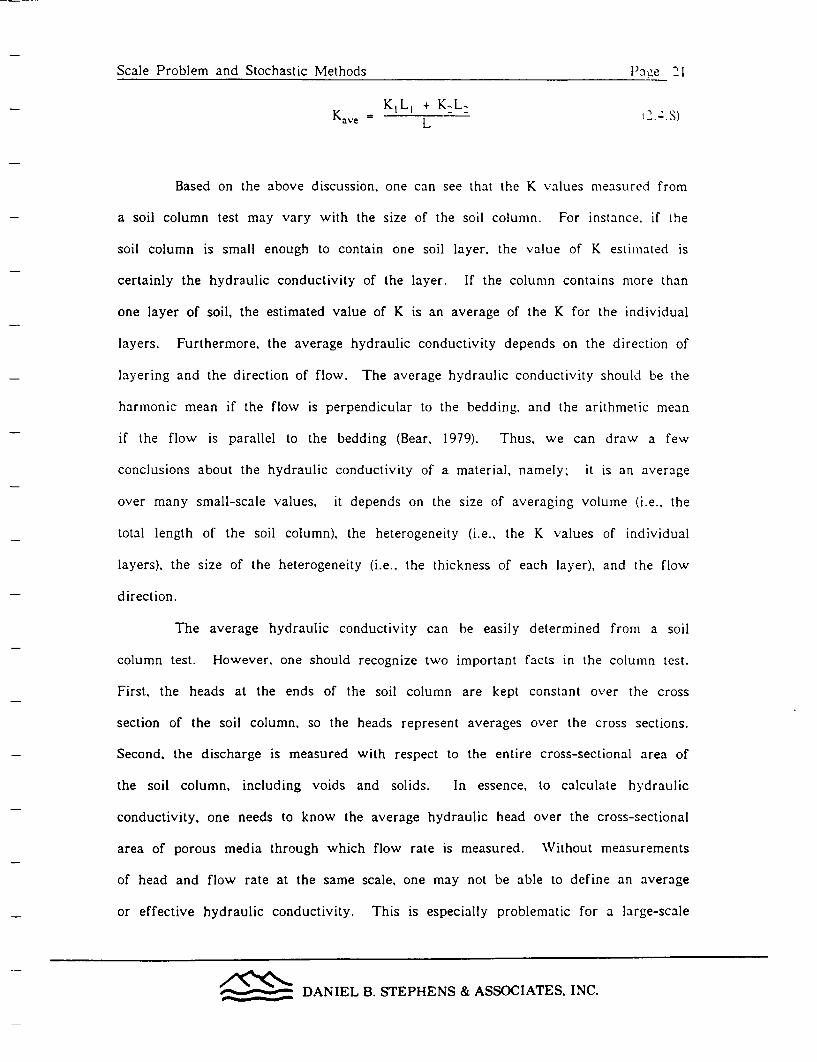
KIL, + K-L,ave L .
Based on the above discussion. one can see that the K values measured from
a soil column test may vary with the size of the soil column. For instance. if the
soil column is small enough to contain one soil layer, the value of K estimated is
certainly the hydraulic conductivity of the layer. If the column contains more than
one layer of soil, the estimated value of K is an average of the K for the individual
layers. Furthermore, the average hydraulic conductivity depends on the direction of
layering and the direction of flow. The average hydraulic conductivity should be the
harmonic mean if the flow is perpendicular to the bedding, and the arithmetic mean
if the flow is parallel to the bedding (Bear, 1979). Thus, we can draw a few
conclusions about the hydraulic conductivity of a material, namely; it is an average
over many small-scale values, it depends on the size of averaging volume (i.e., the
total length of the soil column), the heterogeneity (i.e., the K values of individual
layers), the size of the heterogeneity (i.e., the thickness of each layer), and the flow
direction.
The average hydraulic conductivity can be easily determined from a soil
column test. However, one should recognize two important facts in the column test.
First, the heads at the ends of the soil column are kept constant over the cross
section of the soil column, so the heads represent averages over the cross sections.
Second, the discharge is measured with respect to the entire cross-sectional area of
the soil column, including voids and solids. In essence, to calculate hydraulic
conductivity, one needs to know the average hydraulic head over the cross-sectional
area of porous media through which flow rate is measured. Without measurements
of head and flow rate at the same scale, one may not be able to define an average
or effective hydraulic conductivity. This is especially problematic for a large-scale
________ DANIEL B. STEPHENS & ASSOCIATES, INC.

Scale Problem and Stochastic Methods Page 22
field site. Inasmuch as in the field problem analogous to the column in fligure 2.5,
the hydraulic head measured by a piezometer is generally regarded as a "point"
measurement, and we usually do not have an instrument to measure the total
discharge from a large aquifer. Hence the limitations of the measuring capacity of
our instruments may restrain us from using the averaging rules discussed above. or at
least from using Darcy's equation directly to compute an effective or average
hydraulic conductivity for an aquifer.
2.4.2 Specific discharge. Darcy's law provides us with a method to calculate
the total discharge or flow rate from a soil column, providing that we know the head
gradient and hydraulic conductivity of the soil column. Specific discharge is defined
as the total discharge rate divided by the cross-sectional area of the column. This
means that the specific discharge is an average discharge value over the cross-
sectional area. It does not represent the discharge from individual pores or areas
smaller than the cross-sectional area. It is an average flux through a porous medium,
at a scale at least as large as that of the REV.
2.4.3 Average fluid particle velocity. The average flow velocity of fluid
particles is generally determined by the ratio of total discharge rate to the cross-
sectional area of pore space through which flow occurs. This leads to the definition
of average fluid particle velocity or average linear velocity in groundwater hydrology,
which is:
v = q Q ~~~~~~~~~(2.4.9)ne Ane
where q is the specific discharge and ne is the effective porosity through which flow
occurs. This is an average pore velocity over the total pore area in the cross
section. Consequently, it does not represent the water velocity within individual
DANIEL B. STEPHENS & ASSOCIATES, INC.
Scale Problem and Stochastic Methods Page 23
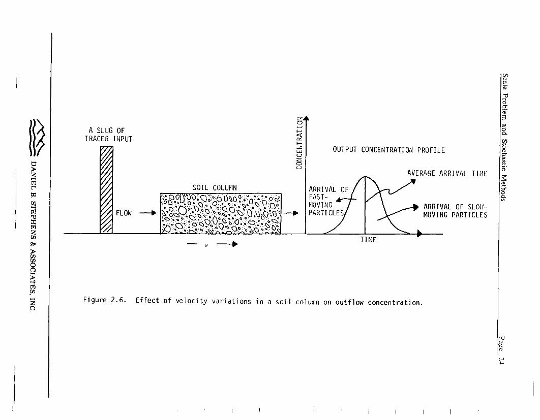
pores, because the areas of individual pores vary. As a result, if one uses the
average fluid particle velocity to determine the arrival of a slug of tracer in the
column test, the time of arrival would be the average arrival time of the tracer
particles. Certainly, some of the tracer particles will move through larger pores and
will arrive earlier than the predicted by the average time, and some of them will lag
behind (Figure 2.6).
Generally, the average fluid particle velocity and the velocity deviations will
vary with the size of the soil sample over which averaging takes place. If the
sample is small enough to contain one soil, the velocity variation in a soil column
tracer experiment, manifested in dispersion or spreading of tracer particle arrival
times, will represent the velocity variation in the pore scale. If the sample is large
enough to include several different soils, it will represent the combined effect of the
variation in velocity among pores and among layers, and so on. Once again the
velocity deviation is scale-dependent.
The average fluid particle velocity which is based on Darcy's law and
effective hydraulic conductivity does not take into account the velocity variations at
scales smaller than the scale at which the average fluid particle velocity is obtained.
Then, how do hydrologists take account of the variation in velocity at the pore-scale
or at any other scale? This question will be answered in the section that deals with
dispersion.
2.4.4. Hydraulic Head. Now let us examine the physical meaning of
hydraulic head in an equivalent homogeneous soil column. In the previous constant
head permeameter examples (Section 2.4.1), a layered soil column was visualized as
an equivalent homogeneous one (Figure 2.5). The effective hydraulic conductivity
can be measured, and for flow perpendicular to the layering it is the harmonic mean
of the two soil layers (equation 2.4.7). Certainly, one can use Darcy's equation and
this effective hydraulic conductivity to determine a head distribution along the
DANIEL B. STEPHENS & ASSOCIATES. INC.
z
Ci2
z
(12
A SLUG OFTRACER INPUT
t/)p
100'
0.OUTPUT CONCENTRATION PROFILE
AVERAGE ARRIVAL THIE
SOIL COLUMN
ARRIVAL OF SLOW-MOVING PARTICLES
- V 0 TI ME
Figure 2.6. Effect of velocity variations in a soil column on outflow concentration.
tLi
(frI(D
III I i Il I
Scale Problem and Stochastic Methods Page 25
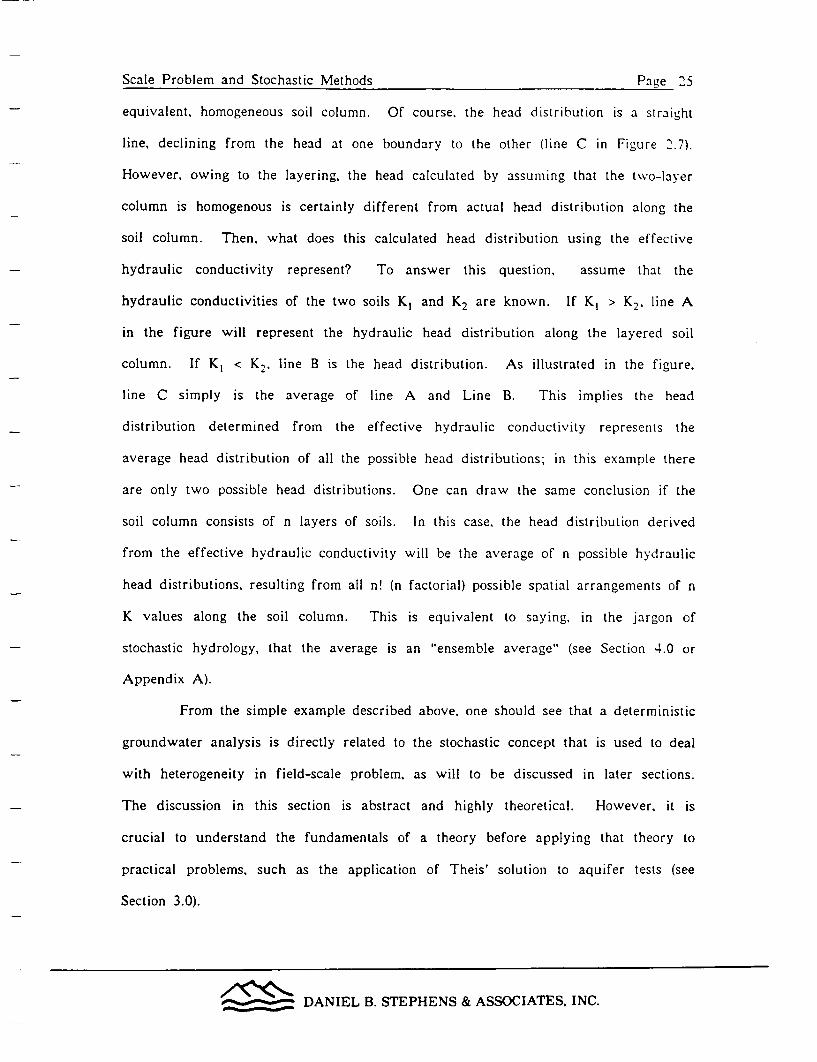
equivalent, homogeneous soil column. Of course. the head distribution is a straight
line, declining from the head at one boundary to the other (line C in Figure 2.7).
However, owing to the layering, the head calculated by assuming that the two-layer
column is homogenous is certainly different from actual head distribution along the
soil column. Then, what does this calculated head distribution using the effective
hydraulic conductivity represent? To answer this question, assume that the
hydraulic conductivities of the two soils K, and K2 are known. If K, > K2. line A
in the figure will represent the hydraulic head distribution along the layered soil
column. If K, < K2, line B is the head distribution. As illustrated in the figure.
line C simply is the average of line A and Line B. This implies the head
distribution determined from the effective hydraulic conductivity represents the
average head distribution of all the possible head distributions; in this example there
are only two possible head distributions. One can draw the same conclusion if the
soil column consists of n layers of soils. In this case, the head distribution derived
from the effective hydraulic conductivity will be the average of n possible hydraulic
head distributions, resulting from all n! (n factorial) possible spatial arrangements of n
K values along the soil column. This is equivalent to saying, in the jargon of
stochastic hydrology, that the average is an "ensemble average" (see Section 4.0 or
Appendix A).
From the simple example described above. one should see that a deterministic
groundwater analysis is directly related to the stochastic concept that is used to deal
with heterogeneity in field-scale problem, as will to be discussed in later sections.
The discussion in this section is abstract and highly theoretical. However, it is
crucial to understand the fundamentals of a theory before applying that theory to
practical problems, such as the application of Theis' solution to aquifer tests (see
Section 3.0).
DANIEL B. STEPHENS & ASSOCIATES, INC.

Scale Problem and Stochastic Methods Page 26
Q
C
A
H-
-JLLj
SOIL 2
Q
0 HEAD
Figure 2.7. Concept of average hydraulic head distribution. Line Ais for K >K2 , line B is for <K2, and line C is for
ave-
DANIEL B. STEPHENS & ASSOCIATES, INC.

Scale Problem and Stochastic Methods Page 27
2.5 Governing Groundwater Flow Equations
Estimating groundwater travel times in porous media requires the knowledge
of the average fluid particle velocity which is determined by the gradient and the
hydraulic conductivity values. Hydraulic gradients in groundwater problems are
derived from hydraulic heads which may vary with time and space. Governing
groundwater flow equations are used to predict the temporal and spatial variations of
hydraulic heads. However, the equations are developed for the specific scales for
Darcy's law and physical properties of groundwater discussed previously.
Consequently, predictions from the equations, i.e., hydraulic heads, represent averages
over some scale as well. Since groundwater travel times and paths are directly
related to the hydraulic head distribution, understanding the meaning of the heads in
equations of different scales is necessary. In the following sections. we will discuss
the development of governing groundwater flow equations for various scales. Then,
we will examine the physical meaning of head values. Meanwhile, some
inconsistencies in the development of the equations which may contribute to
uncertainties in predicting groundwater travel times will be elaborated on Appendix
B.
2.5.1 Three-Dimensional Groundwater Flow Equation. To derive the
governing groundwater flow equation, we start with the mass balance equation.
Consider the mass balance of a stationary control volume at least as large as an REV
(Figure 2.8) whose shape is fixed in space and time. The principle of mass
conservation within this control volume requires that
{ rate of mass accumulation } = { rate of mass in } - { rate
of mass out } (2.5.1)
To apply the principle to the control volume, we begin by considering the pair of
faces perpendicular to the x axis. The rate of mass in through the face at x is
DANIEL B. STEPHENS & ASSOCIATES, INC.

ScaIe Problem and Stochastic Methods Page 28
AZ
x + axx
Figure 2.8.
1By
¼'
Li
A control volume for mass balance.
____t__ DANIEL B. STEPHENS & ASSOCIATES, INC.

Scale Problem and Stochastic Methods Page 29
(pqy)l' /\yAz, and the rate of mass in through the face at x+Ax is (poq,)f,+a lAdz.
Similar expressions may be written for the other two pairs of faces. The rate of
mass accumulation within the volume element is (AXxAvAz) [ant. 3. where n is the
porosity of the control volume. The mass balance then becomes
AxAyAz ap]_Ay<z[(PqX)') x-(pqx)l x+Ax]+ AxAz[(p%, )j -(pqy)l y+Ay]+
Ax/y[(pq,)l z-(pqz)l Z+Lxz] (2.5.2)
By dividing this entire equation by (AxAyAz) and taking the limit
as these dimensions approach zero, we get
anp [apq, apq,, apq, 253at Lax + ay +az J'53
This is the equation of continuity for flow through porous media, which describes
the rate of change of fluid density at a fixed point resulting from the changes in
the mass flux pq (the bold type indicates a vector quantity, ie, a quantity having
both magnitude and directions). Note that replacing the difference equation (2.5.2) by
the partial differential equation (2.5.3) implies all the variables in (2.5.3) are
continuous and differentiable in both space and time coordinates. regardless of
whether the point of interest falls within a pore or solid. That is, the continuum
assumption discussed previously has been used. Using the vector notation, equation
(2.5.3) can be expressed as:
ap -(V pq) (2.5.4)at & ASCTIN
_______DANIEL B. STEPHENS & ASSOCIATES, INC.
Scale Problem and Stochastic Methods Page 30
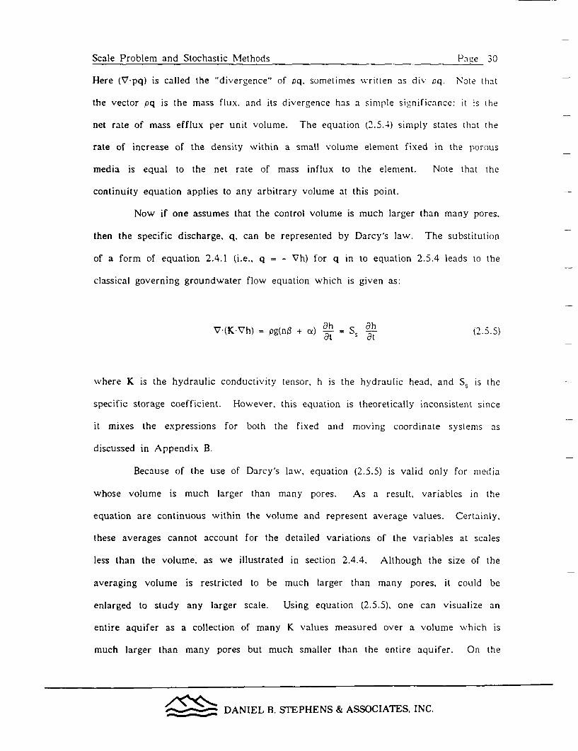
Here (V-pq) is called the "divergence" of pq, sometimes xwritten as div pq. Note that
the vector pq is the mass flux, and its divergence has a simple significance: it is the
net rate of mass efflux per unit volume. The equation (2.5.4) simply states that the
rate of increase of the density within a small volume element fixed in the porous
media is equal to the net rate of mass influx to the element. Note that the
continuity equation applies to any arbitrary volume at this point.
Now if one assumes that the control volume is much larger than many pores,
then the specific discharge, q, can be represented by Darcy's law. The substitution
of a form of equation 2.4.1 (i.e., q = - Vh) for q in to equation 2.5.4 leads to the
classical governing groundwater flow equation which is given as:
V (K Vh) = pg(n3 + ce) ah = Ss ah (2.5.5)at at
where K is the hydraulic conductivity tensor, h is the hydraulic head, and S. is the
specific storage coefficient. However, this equation is theoretically inconsistent since
it mixes the expressions for both the fixed and moving coordinate systems as
discussed in Appendix B.
Because of the use of Darcy's law, equation (2.5.5) is valid only for media
whose volume is much larger than many pores. As a result, variables in the
equation are continuous within the volume and represent average values. Certainly,
these averages cannot account for the detailed variations of the variables at scales
less than the volume, as we illustrated in section 2.4.4. Although the size of the
averaging volume is restricted to be much larger than many pores, it could be
enlarged to study any larger scale. Using equation (2.5.5), one can visualize an
entire aquifer as a collection of many K values measured over a volume which is
much larger than many pores but much smaller than the entire aquifer. On the
_______ DANIEL B. STEPHENS & ASSOCIATES, INC.

Scale Problem and Stochastic Methods Pace 31
other hand, one can enlarge the REV so that the entire aquifer is considered
homogeneous but the flow field remains three-dimensional. By reducing the size of
the control volume, we obtain variables which are more representative of smaller
scale variations within the volume.
2.5.2 Two-Dimensional Depth-Averaged Groundwater Flow Equation.
Generally speaking, the three-dimensional groundwater flow equation is more
representative of real flow fields than one- or two- dimensional equations. However,
it may be impractical because a large number of data and a large amount of
computer time are required for simulating three-dimensional flows in a field- or
regional-scale aquifer system. Sometimes, it may be adequate to conceptualize such a
three-dimensional flow field by a two-dimensional horizontal plane flow phenomenon.
This conceptualization involves taking vertical averages of the three-dimensional
groundwater flow equation. i.e.
zo+b rzo+b
V (K-Vh) dz= J Ss ahdz (2.5.6)Zo Zo
where z0 is the elevation of the bottom of the aquifer, and b is the thickness of the
aquifer Bear, (1979). Integration of (2.5.6) results in a two-dimensional depth-
averaged equation,
V'-(T V'H) _S aHat
where V' is the two-dimensional divergence
DANIEL B. STEPHENS & ASSOCIATES, INC.
Scale Problem and Stochastic Methods Pag~e 32Scale Problem and Stochastic Methods Pasze 32
zo+b
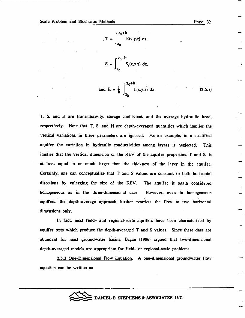
T - J K(x.y.z) dz,
zo+bS . J S5(x.yz) dz.
zo+bIFand H - J h(x~y~z) dz (2.5.7)
T. S. and H are transmissivity, storage coefficient, and the average hydraulic head,
respectively. Note that T, S. and H are depth-averaged quantities which implies the
vertical variations in these parameters are ignored. As an example, in a stratified
aquifer the variation in hydraulic conductivities among layers is neglected. This
implies that the vertical dimension of the REV of the aquifer properties. T and S. is
at least equal to or much larger than the thickness of the layer in the aquifer.
Certainly, one can conceptualize that T and S values are constant in both horizontal
directions by enlarging the size of the REV. The aquifer is again considered
homogeneous as in the three-dimensional case. However, even in homogeneous
aquifers, the depth-average approach further restricts the flow to two horizontal
dimensions only.
In fact, most field- and regional-scale aquifers have been characterized by
aquifer tests which produce the depth-averaged T and S values. Since these data are
abundant for most groundwater basins, Dagan (1986) argued that two-dimensional
depth-averaged models are appropriate for field- or regional-scale problems.
2.5.3 One-Dimensional Flow Equation. A one-dimensional groundwater flow
equation can be written as
_______ DANIEL B. STEPHENS & ASSOCIATES, INC
Scale Problem and Stochastic Methods Pace 33Scale Problem and Stochastic Methods Pace 33~~~~~~~~~~~~~
cx [K (I = s at (5. S)
This equation is equivalent to conceptualizing an aquifer as a soil column (e.g.
Figures 2.5 or 2.6) with flow in the aquifer being strictly unidirectional. If K is
allowed to vary in the x direction, dimensions of the averaging volume (REV) in the
other two directions, i.e. y, and z, are obviously as large as or larger than the width
and thickness of heterogeneities (such as clay lenses) in the aquifer. If K is assumed
constant in the x direction, the averaging volume must be much larger than the size
of heterogeneities in the aquifer. Our scale of interest (such as the size of screen
in a well) is much smaller than the entire aquifer. Such a large-scale averaging
procedure may thus lose too much information pertinent to our interests. Therefore,
this one-dimensional conceptualization may be considered of limited value.
2.5.4 Hydraulic Heads. Based on the discussion above, one can conclude
that a three-dimensional equation (2.5.5) is most realistic. It allows us to describe
aquifers as three-dimensional hydraulic conductivity fields using the small size
average volume. The two-dimensional, depth-averaged equation (2.5.6), however,
ignores the variations in hydraulic conductivity in the vertical direction. A one-
dimensional equation (2.5.8) further averages the hydraulic conductivity variation in
two directions (i.e., horizontal and vertical directions).
Groundwater flow equations for three-, two-, and one-dimensional problems
(2.5.5, 2.5.6, and 2.5.8) allow us to conceptualize heterogeneous aquifers as
homogeneous ones, using an appropriate REV. However, the flow fields (hydraulic
heads) determined by each equation represent different averages. Because of the
homogeneity assumption, the three-dimensional governing flow equation produces an
ensemble-averaged three-dimensional head distribution. In other words, the head
distribution is the average of all possible three-dimensional head distributions, as
_______DANIEL B. STEPHENS & ASSOCIATES. INC.

Scale Problem and Stochastic Methods Page 34
discussed in Section 2.4.4. Note even though the aquifer is considered homogeneous.
the head distribution may retain its three-dimensional characteristics, depending on
type of flow field (i.e., uniform, converging, or diverging flow). Generally. the head
determined by the three-dimensional flow equation for a homogeneous aquifer is
analogous to the water level observed in a piezometer (Figure 2.9), if the aquifer is
truly homogeneous (i.e. heterogeneity exists only at pore-level). However, if the
heterogeneity is much larger than the opening of the piezometer. the head calculated
by the three-dimensional equation with homogeneity assumption will differ from the
one observed in the piezometer. The two-dimensional equation averages three-
dimensional head distributions in the vertical to produce two-dimensional, depth-
averaged heads. The depth-averaged head is equivalent to the water level observed
in a well screened over the entire thickness of the aquifer (Figure 2.9). This depth-
average procedure simply forces the head values along the vertical to be a constant
value which is not identical to the ensemble average, unless the mean flow is parallel
to stratifications. One-dimensional equations further reduce the two-dimensional head
distribution to a one-dimensional one. The head resulting from the one-dimensional
model is analogous to the water level in an excavation ditch which cuts completely
through the aquifer, if there is no flow in the ditch.
As discussed above, each governing equation uses different averaged
hydraulic properties of the aquifer. Each also gives hydraulic head values with
different meanings. As a result, the fluid particle velocity determined from the
averaged heads represents different averages. Moreover, these averages neglect
variations in velocity at scales less than the scale where the averages apply.
Therefore, one may ask: how can one include the effects of these variations smaller
than the averaging scale to obtain a more realistic prediction of groundwater travel
times and paths? We will try to address this equation in the next section that
discusses the dispersion phenomena.
_______DANIEL B. STEPHENS & ASSOCIATES, INC.
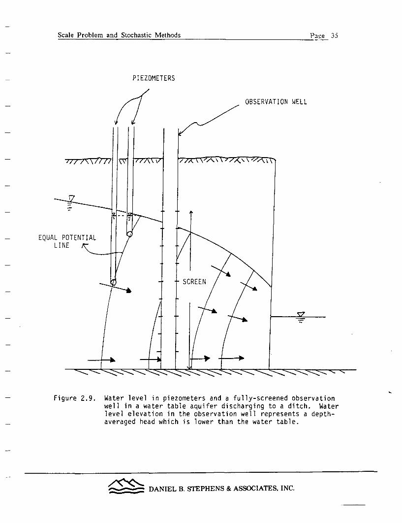
Scale Problem and Stochastic Methods Pave 33Scale Problem and Stochastic Methods Pace 35~~~~~~~~~~~~~~~~~~~~~~~~~~~~~~~~~~~~~~~~~~~~~~~~~~~~~~~~~~~~~~~~~~~~~~~~~~~~~~~~~~~
PIEZOMETERS
OBSERVATION WELL
Figure 2.9. Water level in piezometers and a fully-screened observationwell in a water table aquifer discharging to a ditch. Waterlevel elevation in the observation well represents a depth-averaged head which is lower than the water table.
_____ DANIEL B. STEPHENS & ASSOCIATES, INC.
Scale Problem and Stochastic Methods Page 36
2.6 Hydrodynamic Dispersion
To include the variations in fluid particle motion at scales smaller than the
scale at which the results of the flow equations apply, the concept of hydrodynamic
dispersion must be introduced. However. before hydrodynamic dispersion is
discussed, we will review the basic concept of molecular diffusion, which is
analogous to hydrodynamic dispersion but at a much smaller scale.
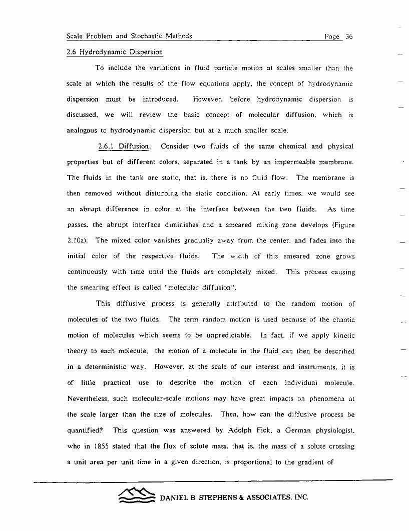
2.6.1 -Diffusion. Consider two fluids of the same chemical and physical
properties but of different colors, separated in a tank by an impermeable membrane.
The fluids in the tank are static, that is, there is no fluid flow. The membrane is
then removed without disturbing the static condition. At early times, we would see
an abrupt difference in color at the interface between the two fluids. As time
passes, the abrupt interface diminishes and a smeared mixing zone develops (Figure
2.10a). The mixed color vanishes gradually away from the center, and fades into the
initial color of the respective fluids. The width of this smeared zone grows
continuously with time until the fluids are completely mixed. This process causing
the smearing effect is called "molecular diffusion".
This diffusive process is generally attributed to the random motion of
molecules of the two fluids. The term random motion is used because of the chaotic
motion of molecules which seems to be unpredictable. In fact, if we apply kinetic
theory to each molecule, the motion of a molecule in the fluid can then be described
in a deterministic way. However, at the scale of our interest and instruments, it is
of little practical use to describe the motion of each individual molecule.
Nevertheless, such molecular-scale motions may have great impacts on phenomena at
the scale larger than the size of molecules. Then, how can the diffusive process be
quantified? This question was answered by Adolph Fick. a German physiologist.
who in 1855 stated that the flux of solute mass, that is, the mass of a solute crossing
a unit area per unit time in a given direction, is proportional to the gradient of
_______ DANIEL B. STEPHENS & ASSOCIATES, INC.

Scale Problem and Stochastic Methods Pag-e 3 7Scale Problem and Stochastic Methods Pace 37
AVERAGED WIDTH
W
7II
-E--
l K IIEtiBRANE
(a)
2D = SLOPE
t
(b)
Figure 2.10. (a) Smearing effect in a tank, and (b)the linear relationship between w2 andtime.
DANIEL B. STEPHENS & ASSOCIATES, INC.

Scale Problem and Stochastic Methods Page 38
solute concentration in that direction. This relationship is generally known as Fl-ek's
Law.
For a one-dimensional diffusion process. Fick's law can be stated
mathematically as
qm - -DM ac (2.6. I)
where qm is the solute mass flux; c, is the mass concentration of diffusing solute;
DM. is a coefficient of proportionality called the diffusion coefficient, and the minus
sign indicates transport is from high to low concentrations. Fick's law is similar to
Darcy's law in which the mass flux of water is related to the conductivity and
hydraulic gradient. Similar to the hydraulic conductivity, the diffusion coefficient is
a quantity averaged over a volume much larger than many molecules and the motion
of individual molecules is ignored.
To illustrate the concept of averaging in a diffusion process, we will
reexamine the case where two fluids are separated by a membrane. As mentioned
earlier, the width of the mixing zone grows with time. Here, the width is defined as
an average width of the mixing zone over the depth of the tank because the width
may vary from depth to depth as shown in Figure 2.10a. This average is equivalent
to the depth-average procedure discussed in section (2.5.2). If one repeatedly carries
out the same experiment, the depth-average width may be different from one
experiment to another because of the random motion of the molecules. However, if
one averages the depth-averaged width of all the experiments, one obtains an average
width which is an ensemble average, i.e., average over many possible outcomes. As
a matter of fact, if the square of the ensemble-average width, w2, is plotted as a
function of time, a linear Telatiornship is found (Figure 2.10b). The slope of the line
DANIEL B. STEPHENS & ASSOCIATES, INC.
Scale Problem and Stochastic Methods Page 39
is generally related to the diffusion coefficient by
dw2 =D (2.6.2)
In other words, the diffusion coefficient, DM. describes the rate of growth of the
average width of the mixing zone over the depth of the tank, and over many
experiments. It certainly does not intend to depict the rates at each depth and each
experiment. Therefore, the coefficient of diffusion is merely a mean parameter. In
view of the fact that our measuring devices, and human vision are limited, and the
fact that repeated experiments are impractical, a diffusion coefficient obtained in one
experiment is often considered adequate. This assumption implies the equivalence
between the depth-average and the ensemble average (i.e. an ergodicity assumption;
see Appendix A and Section 4.1). Since Dm is an average value, one should not
expect that the concentration of the colored fluids can be predicted by using the
diffusion coefficient at scales much smaller than the scale at which DM is derived.
Furthermore, one should not expect that the concentration predicted by the diffusion
concept will be identical to the one observed in a single experiment.
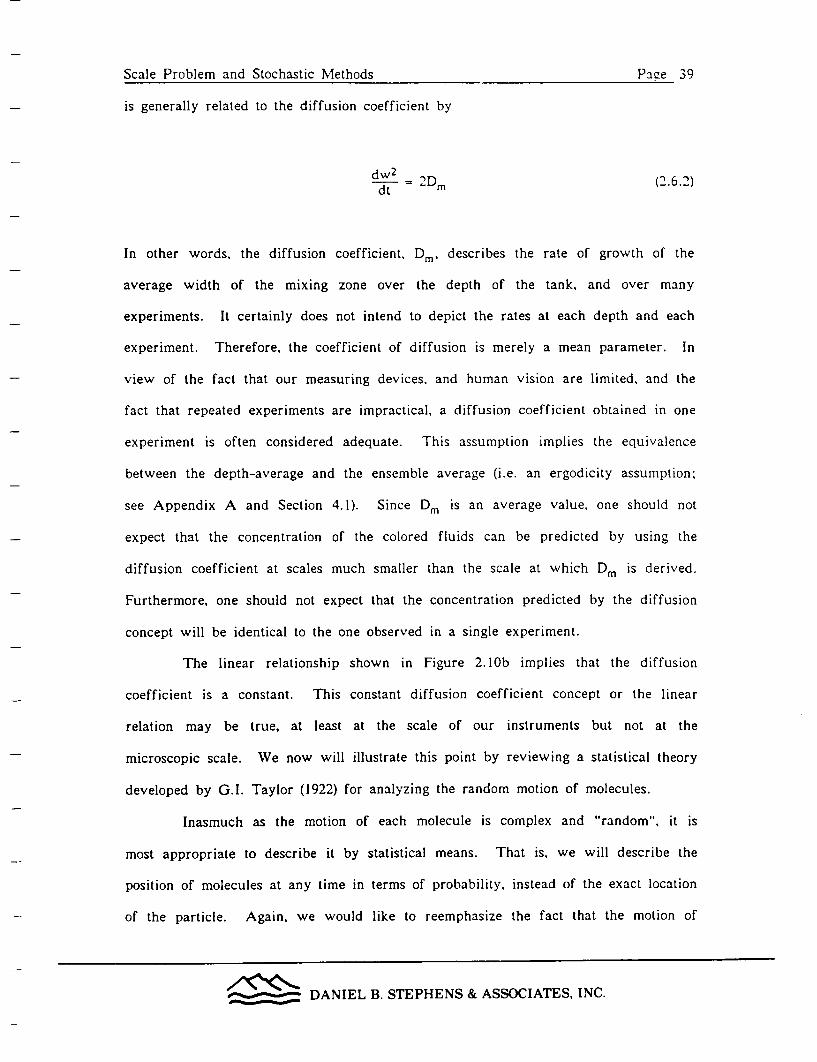
The linear relationship shown in Figure 2.10b implies that the diffusion
coefficient is a constant. This constant diffusion coefficient concept or the linear
relation may be true, at least at the scale of our instruments but not at the
microscopic scale. We now will illustrate this point by reviewing a statistical theory
developed by G.I. Taylor (1922) for analyzing the random motion of molecules.
Inasmuch as the motion of each molecule is complex and "random", it is
most appropriate to describe it by statistical means. That is. we will describe the
position of molecules at any time in terms of probability, instead of the exact location
of the particle. Again, we would like to reemphasize the fact that the motion of
_______ DANIEL B. STEPHENS & ASSOCIATES, INC.

Scale Problem and Stochastic Methods Pace -O
molecules is deterministic but too complex for us to use any deterministic approach.
Furthermore, we are not interested in how individual molecules move. Based on
these reasons, we conceptualize the deterministic movement of molecules as a random
process. To carry out this statistical analysis of random motion, we will assume that
the velocity of a diffusing molecule is a stationary stochastic process in time
(Csanady, 1973). This means that we do not know the velocity of the molecule at
any time, but we could determine all the possible velocity values from the known
statistical properties of the process, such as mean, variance, or probability distribution
of the velocity (for definitions of statistical terms refer to Appendix A). Without loss
of generality, we may say that the mean and variance of the velocity of a molecule
are constant in time: i.e.,
E[v(t)] = constant = 0
and E[v2 (t)] = constant = E[v 2],
respectively, where E[ ] stands for the expected value which represents the
probablistic average of a random variable. Another important statistical parameter
characterizing a stationary stochastic process is its autocorrelation function. Rvv(7),
where T is the time lag between two times, t and t+T. The autocorrelation function
of the velocity history of a molecule may be regarded as measuring the persistence of
the velocity of a molecule throughout a period of time (Appendix A). In other
words, it is a measure of the correlation of the velocities of a molecule between any
time interval, T. Thus, the velocity autocorrelation function is defined as:
RV(T) = E[ v(t) v(t + T) 1 (2.6.3)E[ v(0)2]
_______ DANIEL B. STEPHENS & ASSOCIATES, INC.

Scale Problem and Stochastic Methods Page 41
where E[v(0)21 is the variance of velocity. In a stationary stochastic process. the
autocorrelation function is independent of time t but dependent on the time lam.
In the case of the velocity history of a diffusing molecule. such an autocorrelation
function implies that once the molecule possesses a certain velocity, a short time T
later it is still likely to have a velocity of a similar magnitude and sign. For a given
time lag T. the velocity covariance, E[v(t)v(t+r)] may be formed, which evidently tends
to E[v2] as T -O. However, after a long enough time T, the molecule tends to 'forget'
the velocity at time t, in the sense that the value of v at t+r will be quite
independent of v(t). That is, at t=O, R,(T)=1, while as T approaches x, RVV(T)
becomes 0, as shown in Figure 2.11.
The displacement of an individual diffusing fluid or tracer molecule at
any time, t, can be related to its velocity by
x(t) = {v(s)ds (2.6.4)
where x is the position. Now we imagine that there is more than one molecule
moving "randomly" in fluid space. We further assume that the statistical
characteristics (i.e., mean, variance, and covariance) of molecule's velocities are the
same. After a period of time, the location of each molecule would, of course, be
different. However, these molecules will spread around x=0,
E[x(t)] = I E[v(s)] ds = 0 (2.6.5)
because in a static system the mean velocity. E[v], is zero. As shown in Figure 2.10
_______ DANIEL B. STEPHENS & ASSOCIATES, INC.

Scale Problem and Stochastic Methods P-AsTA AnAl
1.0
0
4-)
La
0)
0
4-)
e-l
Time Lag
Figure 2.11. A hypothetical velocity autocorrelation function.
DANIEL B. STEPHENS & ASSOCIATES, INC.

Scale Problem and Stochastic Methods Page 43
and equation 2.6.2, the spreading, the deviation of the position of a molecule from
the mean position, at time t can be quantified by x(t)2. The rate of change of xU)
may then be written as:
t+T
dx2(t) = 2x 4d = 2 I v(t) v(t+s) ds (2.6.6)dt xdt
Since there are a large number of molecules, the average rate of change of x2(t) of
all the molecules can be obtained by taking the expected value of (2.6.6) and the
result is:
t+T
dEtx2L 2 Ejv2] f R,(T)dT (2.6.7)
where E[x2] is the variance of the molecule positions which is equivalent to the
average width squared, w2 , in equation (2.6.2). The left-hand side of equation (2.6.7)
represents the rate of change in variance of the molecule positions or 2Dm as shown
in equation (2.6.2). In other words, the molecular diffusion coefficient, DM. is
directly related to the molecules' velocity autocorrelation function and it varies with
time. However, due to numerous collisions with other molecules, the velocity of a
molecule at time t+T tends to forget its velocity at t, as T becomes large. For
simplicity, we assume that the velocity autocorrelation function takes the form:
R,,(T) - e-r (2.6.8)
where /3-1 is considered as the persistence time for the velocities of the diffusing
.11~~ DANIEL B. STEPHENS & ASSOCIATES, INC.
Scale Problem and Stochastic Methods Page -4
molecules. This means that, on the average, molecules tend to forget their previouls
velocities after a period of time p3'. This velocity autocorrelation function is shown
in Figure 2.11 as a function of
The integral of R,(7) on the right hand-side of equation (2.6.7) represents
the area under the curve bounded by 0 and t+r. It should be evident from Figure
2.1! that the value of the integral will increase initially but will approach a constant
at large values of t+r, or t+T approaches oo. This result implies the rate of spreading
of the diffusion molecules at large value of T will be a constant according to
equation (2.6.7). As a result, the diffusion coefficient, which is half of the rate of
change in E[x2 ], will increase initially but at t>>,-I it tends to stabilize. For a
particle of a radius, 10-4 cm. the persistence time, 031, is about 1.4x10⁻⁸ seconds
(Csanady. 1973). Since the scale of our observation is likely much greater than
I.4xIo-8 seconds, the time-dependent portion of the diffusion coefficient can be
neglected and the diffusion coefficient can virtually be treated as a constant value.
For much smaller scales of observations this may not be the case.
2.6.2 Advection-Diffusion Equation. Now suppose that an ideal fluid with a
tracer is moving in a frictionless pipe. In this hypothetical frictionless pipe, there
are no velocity variations caused by friction between the fluid and the wall of the
pipe, so that the velocity recorded by small instruments is constant across the cross-
section of the pipe, because friction does not exist. However, at the molecular level,
molecules move at different velocities. The size of our instruments for measuring a
flow velocity is generally much greater than the size of molecules. Obviously, the
velocity we determined from the measurement is an average value over many
molecules. This average velocity does not consider the variation in velocity of
molecules. For example, consider a tracer experiment in a frictionless pipe (Figure
2.12a). If 10,000 tracer molecules are simultaneously released at one end of the pipe
at time, to, then at various times the discharge at the other end of the pipe is
_______ DANIEL B. STEPHENS & ASSOCIATES, INC.
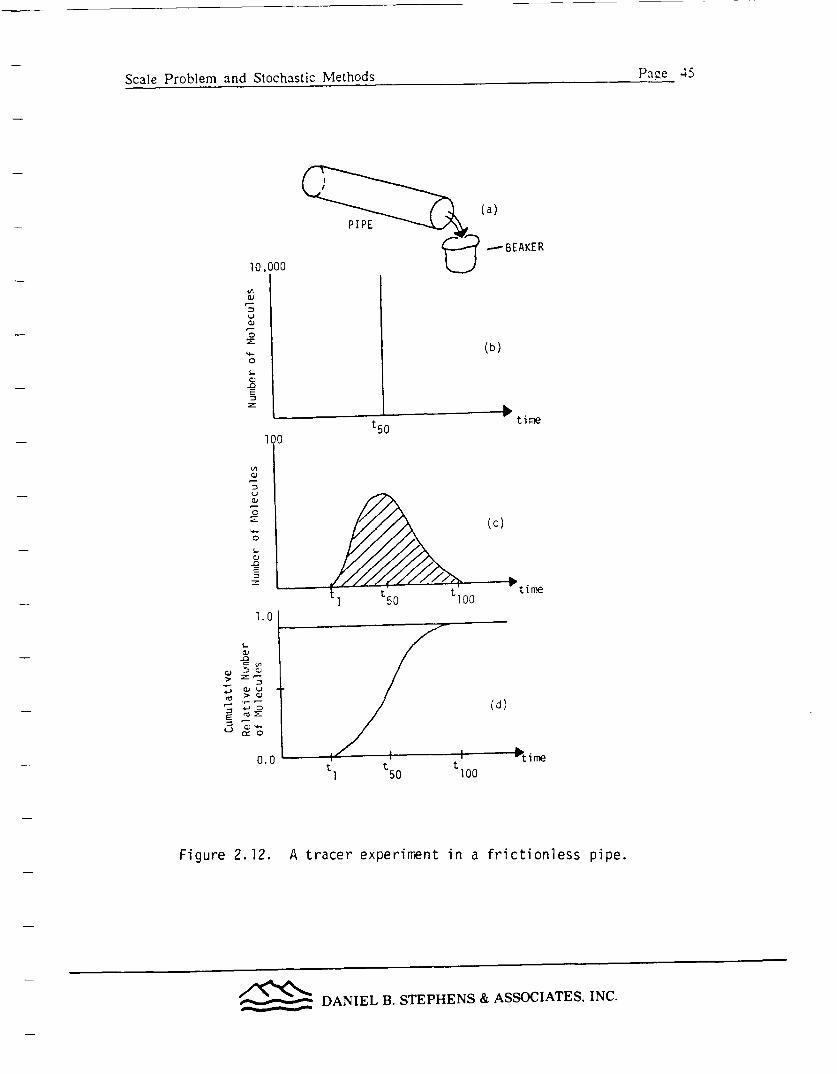
Scale Problem and Stochastic Methods Pace 45
PIPE
10,000
12,oJ
Li0z0
(a)
BEAKER
(b)
.n
I tile
t50 im
0
C.,
1. 0
(c)
time
*0
L)
a.
-o
a!.,
0.0
(d)
t100
Figure 2.12. A tracer experiment in a frictionless pipe.
,______ DANIEL B. STEPHENS & ASSOCIATES, INC.
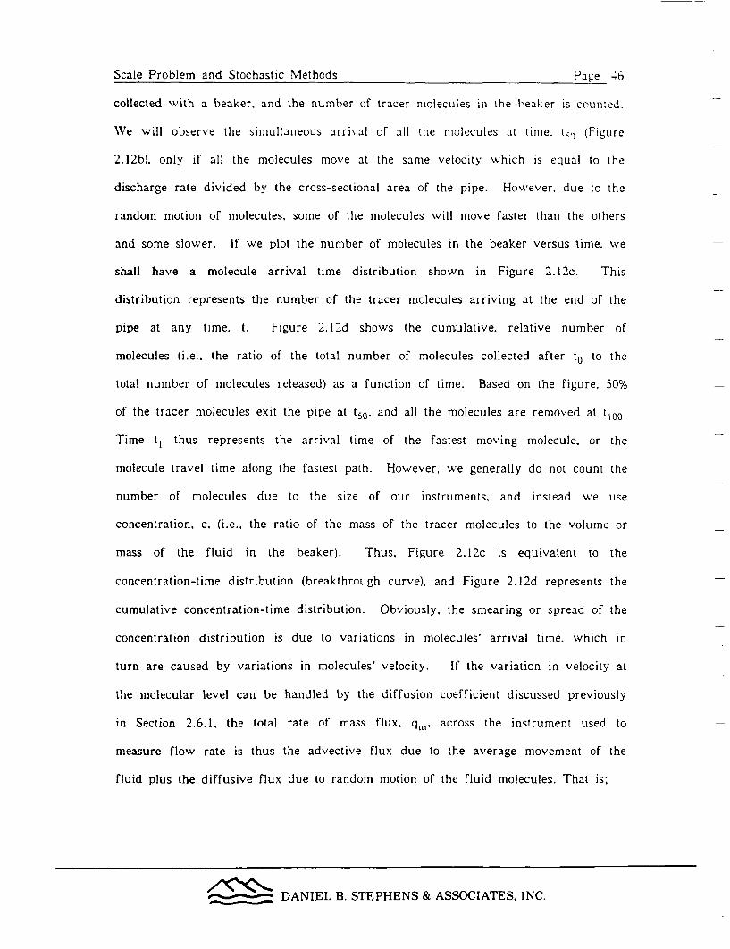
Scale Problem and Stochastic Methods Pave 46
collected with a beaker, and the number of tracer molecules in the beaker is cnunted.
We will observe the simultaneous arrival of all the molecules at lime. t. (Figure
2.12b), only if all the molecules move at the same velocity which is equal to the
discharge rate divided by the cross-sectional area of the pipe. However, due to the
random motion of molecules, some of the molecules will move faster than the others
and some slower. If we plot the number of molecules in the beaker versus time, we
shall have a molecule arrival time distribution shown in Figure 2.12c. This
distribution represents the number of the tracer molecules arriving at the end of the
pipe at any time, t. Figure 2.12d shows the cumulative, relative number of
molecules (i.e., the ratio of the total number of molecules collected after to to the
total number of molecules released) as a function of time. Based on the figure, 50%
of the tracer molecules exit the pipe at t50. and all the molecules are removed at tlo,.
Time t1 thus represents the arrival time of the fastest moving molecule, or the
molecule travel time along the fastest path. However, we generally do not count the
number of molecules due to the size of our instruments, and instead we use
concentration, c, (i.e., the ratio of the mass of the tracer molecules to the volume or
mass of the fluid in the beaker). Thus, Figure 2.12c is equivalent to the
concentration-time distribution (breakthrough curve), and Figure 2.12d represents the
cumulative concentration-time distribution. Obviously, the smearing or spread of the
concentration distribution is due to variations in molecules' arrival time, which in
turn are caused by variations in molecules' velocity. If the variation in velocity at
the molecular level can be handled by the diffusion coefficient discussed previously
in Section 2.6.1. the total rate of mass flux. qm. across the instrument used to
measure flow rate is thus the advective flux due to the average movement of the
fluid plus the diffusive flux due to random motion of the fluid molecules. That is;
______ DANIEL B. STEPHENS & ASSOCIATES, INC.

Scale Problem and Stochastic Methods Pa ate 4 7
qm = vc + [ -Dm O
where v is the average velocity of the fluid, and c is the concentration of tracer.
The product term vc represents the advective tracer flux and Dmac/ax represents the
diffusive flux. When (2.6.9) is substituted into the equation for conservation of mass
(similar to equation 2.5.4) in one dimension, we obtain the advection-diffusion
equation:
cc + v cc DM a2c (2.6.10)
where the second term on the left hand side of the equation represents the advection
effect and the term on the right hand side of the equation represents the diffusion
effect due to random motion of molecules. Thus, a concentration breakthrough curve
which is the solution of Equation 2.6.10 in time domain reflects the arrival time of
the tracer molecules. The molecular diffusion coefficient is simply a "fudge factor"
accounting for velocity variations of molecules at a scale much smaller than the pipe.
Equation (2.6.10) is developed for tracer movement in a frictionless pipe. In
the case where the wall of the pipe is not smooth but rough, velocities measured at a
scale much larger than many molecules but smaller than the cross-section of the pipe
(say, continuum scale in fluid mechanics) will vary across the cross-section of the
pipe. The velocity is likely maximal in the center of the pipe and is minimal near
the wall. This implies that the velocity determined by a discharge rate divided by
the cross-sectional area of the pipe represents an average velocity value which
neglects the velocity variation across the cross-sectional area due to friction.
Furthermore, it also neglects the velocity variations among individual molecules.
________ DANIEL B. STEPHENS & ASSOCIATES, INC.
Scale Problem and Stochastic Methods Pave -8
Now, if we assume that the velocity variations at scales smaller than the crnss-
sectional area of the pipe and those at the molecular scale can be described by Fick's
law as in the molecular diffusion process. then equation (2.6.10) is valid for this case
as well. However. the diffusion coefficient, Din. in equation (2.6.10) is replaced by a
dispersion coefficient, Dd, which lumps together velocity variations at both the
molecular scale and the continuum scale. Of course, the velocity. v, in equation
(2.6.10) represents the average over the cross-sectional area. The concentration, c,
then represents the total mass of a tracer in a volume of fluid discharging from the
cross-sectional area of the pipe. Generally. this approach is valid for tracer
movement in a long pipe as shown by G.I. Taylor (1953).
Following the above concept, surface-water hydrologists have frequently
applied equation (2.6.10) to determine tracer movement in large-scale water bodies
such as streams, rivers, estuaries, and oceans. Various successes have been reported
in the literature for instance Fischer et al., (1979). Regardless of the validity of
equation (2.6.10) for large-scale problems, the most important feature of the equation
is that the parameters have different physical meanings, depending on the scale.
Moreover, the dispersion coefficient always represents the effects of velocity
variations at scales smaller than the scale at which the average velocity is defined.
2.6.3 Hydrodynamic Dispersion in Porous Media. Now consider flow in a
porous medium (for example, a soil column). At the molecular level, each molecule
has its own velocity. At the scale of a single pore, the velocity averaged over many
molecules may not be constant over the pore space because of the roughness of the
wall of the pore, just like flow in a frictional pipe. At the scale larger than a
single pore variations in pore size, in addition to tortuosity of pore channels, will
then cause an additional velocity variation. As discussed previously, the average
fluid particle velocity defined in groundwater hydrology is the average value over
many pores or heterogeneities of many different scales, depending on the size of the
_______ DANIEL B. STEPHENS & ASSOCIATES, INC.

Scale Problem and Stochastic Methods Page 49
control volume. The average fluid particle velocity does not take velocity variations
at different scales into consideration. To account for the variation in velocity due to
random motion of molecules, roughness of the pore walls, and the variation in size of
pores and tortuosity in a flow path. groundwater hydrologists borrowed the
advection-diffusion concept. In other words, in order to conserve mass. the mass
flux which is not considered by the average fluid particle velocity is lumped into the
dispersive flux term, similar to the way molecular diffusive flux was treated in the
advection-diffusion process. The smearing effect due to the variation in velocity at a
scale larger than the molecules. but smaller than the scale used to determine the
average fluid particle velocity is then attributed to hydrodynamic dispersion.
Therefore, the classic advection-diffusion equation (2.6.10) may then be directly
applied to solute transport in porous media. However, the coefficient of
hydrodynamic dispersion is used in lieu of the diffusion coefficient to represent the
coefficient of proportionality between the mass flux and concentration gradient. The
hydrodynamic dispersion coefficient thus includes the effect of variation in velocity
at many different scales (from the molecular scale to the scale at which the average
linear velocity is defined.) This approach is identical to convection-dispersion
approaches used by surface-water hydrologists in dealing with solute transport in
streams, rivers, and estuaries. However, causes of velocity variations or mechanisms
of dispersion are different.
2.6.4 Mechanisms of Dispersion in Porous Media. Mixing of tracer particles
due to dispersion is primarily an artifact related to the scale of averaging. In the
REV, the hydraulic conductivity and porosity are assumed to be constants
representing the average values over the volume. Consequently, the velocity
determined from these parameters represents an average over the volume. This
velocity describes the average solute movement as a piston type of displacement
which exhibits a sharp interface with the fluid. Smearing effects observed in the
DANIEL B. STEPHENS & ASSOCIATES, INC.
Scale Problem and Stochastic Methods Page 30
experiments are attributed to mixing due to subscale velocity variations within the
REV which are treated as the dispersion process. Since the size of the REV varies
with the scale of heterogeneity, mechanisms of dispersion are accordingly classified
by the scale of heterogeneity.
At the microscopic scale, mixing is caused by random motion of fluid
molecules. This process is called diffusion. At the laboratory scale, mixing is a
result of the combined effects of diffusion and velocity variation within pores, among
pores, and tortuous flow channels. This type of mixing is generally defined as local
dispersion. If the concentration of tracer particles is measured in fully penetrating
observation wells and one uses a two-dimensional depth-average flow and transport
model to simulate the process, then the field-scale dispersion reflects mixing due to
groundwater velocity variations between and within distinct hydrogeologic units, in
addition to molecular diffusion and local dispersion. This type of dispersion is
sometimes called two-dimensional macrodisperison (Gelhar et al., 1979). The term,
macrodispersion. is also used in three-dimensional flow situations if one treats the
entire aquifer as a homogeneous one. However, the two-dimensional macrodispersion
is different from the three-dimensional one in the fact that it also includes the
effects of averaging three-dimensional flow fields into two-dimensional fields (see
section 2.5). Therefore, the mechanics causing dispersion vary with the scale of
averaging.
2.6.5 Dispersivity. The dispersion concept in groundwater hydrology should
become clear by now. Overall, the dispersion coefficient is merely a parameter in
the classic convection-dispersion equation used to include variations in velocity at
subscales. However, velocity variations are not controlled only by the heterogeneity
at different scales of porous media, but also by the flow fields (directions of flow.
and magnitudes of mean velocities). For example, consider an aquifer consisting of
three homogeneous layers with equal thicknesses and with hydraulic conductivities.
_____ DANIEL B. STEPHENS & ASSOCIATES, INC.

Scale Problem and Stochastic Methods Page 51
K, - 10 cm/day, K. = 1cm/day, and K3 = 100 cm/day. For simplicity. w.e will
assume porosity values of the three layers are the same and equal to 0.5. If a
constant hydraulic head gradient 0.01 is imposed on each layer. the average fluid
particle velocity for layers 1. 2, and 3 is 0.2. 0.02, and 2 cm/day, respectively. The
average velocity over the three layers is 0.74 cm/day and the variance is 1.2
cm2/day2. Now, if the gradient is increased to 0.1. the velocities are 2, 0.2. and 20
cm/day for layers 1, 2, and 3, respectively. The mean velocity is then 7.4 cm/day
and variance is 119 cm2/day2 . This simple example illustrates that velocity
variations depend on the magnitude of gradient or mean velocity, as well as the
hydraulic conductivity variation. Therefore, the hydrodynamic dispersion coefficient
depends not only on the physical characteristic of porous media but also on the flow
characteristics.
Inasmuch as flow is likely to vary with time and boundary conditions, how
can this hydrodynamic dispersion coefficient be determined so that one can predict
solute movement in porous media? One way to determine this parameter is to fit, by
trial and error, the solution of the convection-dispersion equation to the results of
tracer experiments. However, in a sense, the dispersion coefficient becomes a
parameter which may vary from one experiment to another experiment even in the
same porous medium, owing to differences in mean pore velocity. For predictive
purposes, such an approach is not suitable.
To overcome this difficulty, many tracer experiments at the laboratory scale
have been done in the past. The results of the experiments showed that the
dispersion coefficient, Dd, is linearly proportional to the average velocity (Bear. 1979):
Dd = Ov (2.6.11)
where v is the average velocity over the laboratory sample and a is the dispersivity.
DANIEL B. STEPHENS & ASSOCIATES, INC.

Scale Problem and Stochastic Methods Pace 52
For homogenous laboratory soil columns, the dispersivity can be further related to the
particle size of porous media, and thus. can be considered constant. Because the
dispersivity is a property of the medium, predicting movement of solutes in a porous
medium under different flow fields now becomes possible.
2.6.6 Scale-Dependent Dispersivity. Taylor's (1922) analysis (Section 2.6.2)
showed that the rate of spreading of molecules grows with time or distance because
of the molecules' velocity persistence. However, the rate reaches a constant value in
a relatively short period of time and distance compared to the measuring capacity of
our instruments. As a result, molecular diffusion can virtually be represented by
Fick's law (equation 2.6.1) with a constant diffusion coefficient.
By the same token, the spreading of a tracer plume in homogeneous soil
columns will grow with time and distance because of the persistence of fluid particle
velocity. This velocity refers to the velocity of a volume of water that is much
larger than many molecules but smaller than the size of a pore. However, the
persistence diminishes due to changes in pore geometries and mixing with water from
other flow paths as the volume of water moves through many pores. Since the size
of pores in soils is small compared to the size of the REV of a soil column, the
classic convection-dispersion equation with a constant dispersion coefficient (or
constant dispersivity) is generally considered adequate to describe solute transport in
homogeneous soil columns.
In field scale problems. the effects of heterogeneity on velocity variations are
controlled by large-scale heterogeneities such as clay lenses, facies changes, and
layerings of sediments. If we assume that by averaging the hydraulic properties, the
field-scale aquifer is, in effect, homogeneous, and we use the dispersion concept to
represent the effect of the heterogeneity on solute transport, we would expect the
dispersion coefficient to grow with distance and reach a constant value at some
distance, as in the molecular diffusion process predicted by Taylor (1922) and
________ DANIEL B. STEPHENS & ASSOCIATES, INC.

Scale Problem and Stochastic Methods Page 53
observed in homogeneous soil column tests. However. a problem arises from the fact
that the size of heterogeneities (such as clay lenses) at the field-scale is many times
larger than the size of irregular pore channels in soil columns. The travel distance
which is sufficient to allow the solute particles to "forget" the influence of the
previous velocity may thus be many times larger than the size of clay lenses or
layerings. Furthermore. this distance is generally much larger than the length of our
field tracer experiments. As a consequence, the dispersivity values estimated from
the field tracer tests seem to grow with travel distance or time (Figure 2.13). This
phenomenon is known as the scale-dependent dispersion. It should be evident by
now that such a scale-dependent dispersion is a result of the scale of heterogeneity,
the scale of averaging, and the scale of observation.
Many theories accounting for the scale-dependent dispersion have been
developed in the past decade for example; Gelhar and Axness, (1983), Neuman et al.,
(1986), Dagan, (1987), Matheron and De Marsily, (1980), etc. Field experiments to
validate the theory of scale-dependent dispersivity in aquifer systems are currently in
progress at several locations in North America, for example, at the Borden land-fill in
Canada (Sudicky, 1986 and Feryberg. 1986) and in Mississippi, (Betson, et al. 1985).
DANIEL B. STEPHENS & ASSOCIATES, INC.

4Z-1a Prnhlprn nnri Stochastic Methods TPace 54o tals . In-- e
1000
100E-
0Li
C)
C=1.
n
I-
.0110 100 1000 10,000 100,000
SCALE (m)
Figure 2.13. Data showing scale-dependent dispersivity (Gelhar, 1986).
_____ DANIEL B. STEPHENS & ASSOCIATES, INC.
Scale Problem and Stochastic Methods Page 55
2.7 Fracture Systems
In the previous sections of the review, we focused on laws and equations
for flow and transport in porous media where large scale features such as fractures
do not exist. Such media are representative of most aquifers which consist of
unconsolidated sediments. However, most of the geologic materials at the proposed
nuclear waste repository sites are generally consolidated sediments, volcanic or
crystalline rocks. These geologic materials contain many fractures resulting from
recent or past tectonic activities. Since groundwater flows through not only the rock
matrix but also fractures, one certainly has to consider the effects of fractures in
order to determine the groundwater travel times and paths in such geologic materials.
Generally speaking, flow and transport phenomena in fractured rock are not as well
understood and characterized as in porous media. This problem can be attributed
partially to scale problems similar to those in porous media. That is, fractures are
too small to be considered as discrete flow channels but too large to be considered as
pore channels in porous media. In addition, the flow regime in fractures may vary
from laminar to turbulent flow in which the classic groundwater flow equation based
on Darcy's law is not valid. In the following sections, we will examine recent
developments in conceptualization of flow and transport in such media under both
saturated and unsaturated conditions.
2.7.1 Flow in Saturated Fractured Rocks. In fractured rocks, the size of a
fracture is generally larger than the size of pores. The density of fractures at the
macroscopic level, however, is much lower than the density of pore spaces. One has
to enlarge the size of the REV defined for porous media in order to visualize
fractured rock as a equivalent porous continuum at a large scale. In other words,
the size of the REV for fractured rocks has to contain many fractures in the same
way that the size of the REV for porous media must be much larger than many
pores. Similarly, the detailed spatial distribution of individual fractures inside the
DANIEL B. STEPHENS & ASSOCIATES, INC.
Scale Problem and Stochastic Methods Page 56
REV is ignored. However. if the knowledge of a detailed spatial distribution of
fractures is available, and the behavior of flow in each fracture is what we are
interested in. we may treat fractures as distinct flow channels embedded in a porous
medium. The individual fracture is then visualized as a continuum with a smaller
REV which ignores the much smaller scale flow channels within each fracture.
Evidently, the size of the REV for individual fractures is not the same as that for
the rock matrix.
Based on the discussion above, we can now classify the approaches of
modeling flow and transport in fractured rocks into the continuum approach and the
discrete approach. The continuum approach assumes that one can enlarge the REV
so that the flow behavior in both the fracture and the porous matrix can be
conceptualized as a flow system in an equivalent porous medium. This implies that
the hydraulic properties of such an REV represents averages of the properties of the
fractures and the rock matrix within the REV. Again, the detailed flow regimes in
both fractures and rock matrix are ignored.
This continuum approach can be further divided into the single network
approach and the double network approach. Such a division is necessary in
fractured rock formations. In porous media, it is generally agreed that solids are
impermeable and do not interact with the fluid in the void space. Thus, hydraulic
conductivity is defined over many pores only. However, this may not be the case in
a fractured rock system where both the fracture and the rock matrix are considered
conductive. In a steady state flow situation, the conductivities of both the fractures
and rock matrix may be represented by the notion of equivalent hydraulic
conductivity. As a consequence. a single network approach is adequate. In this
approach, a fractured medium is represented by a single network in which the
hydraulic properties are averaged over both the fracture and the rock matrix. Thus,
the general governing flow equation is written as:
DANIEL B. STEPHENS & ASSOCIATES, INC.

Scale Problem and Stochastic Methods Page 37
v (K Vh) = as, (2.7. 1)
where K, S.. and h represent the average values of hydraulic conductivity, specific
storage, and head over the fracture and the rock matrix within the volume of the
REV, respectively. For steady state conditions, the right-hand side of equation 2.7.1
is zero. Although the hydraulic properties of such a REV are the averages over
both the fracture and the rock matrix, they are dominated by the properties of
fractures, and the influences of the porous matrix properties are negligible. (This is
especially true for hydraulic conductivity, which is perhaps the most important
property controlling groundwater travel time). Thus, this approach assumes that an
equilibrium between the flows in both fractures and rock matrix exists. Wvhich may
not be valid for most cases.
With the single network approach, one may conceptualize a large-scale
fractured geologic formation as a heterogeneous continuum or a stochastic continuum
if heterogeneities are represented by stochastic processes (Neuman, 1987). Because the
volume over which the averaging takes place may contain several fractures and a
vast number of pores in the rock matrix, the spatial distribution of the hydraulic
properties thus becomes smooth and differentiable. The classic partial differential
equations for flow in heterogeneous porous media can now appropriately applied.
In the transient state, owing to the relatively small storativity in fractures.
the response of the fracture to pressure (or head changes) is much faster than in the
matrix. The interaction between the fracture and the porous rock matrix becomes
important. It therefore becomes necessary to define, inside the REV, two separate
networks: one representing fractures and the other the rock matrix. Each network
within the REV is considered a homogenous continuum. The spatial distribution of
fractures or the rock matrix is not required to be specified within the REV. This
_______DANIEL B. STEPHENS & ASSOCIATES, INC.
Scale Problem and Stochastic Methods Pave 3S
conceptualization is the so called double network or dual porosity model.
The double network approach has been used by many investigators such as
Barenblatt et al. (1960). Warren and Root, (1963), Kazemi. (1969), Zhang. (1 982),
Huyakorn et al. (1983), and Moench (1984). The approach assumes that hydraulic
responses of an REV result from two flow systems. One represents the flow in the
rock matrix network, and the other the fracture network. Flow in each network is
described by a governing flow equation. The influences of fractures on the flow
regime in the rock matrix, or vice versa, are then entered as sink or source terms in
the flow equations. More specifically, the governing differential equation for flow in
the fracture network is assumed to be described by the classic groundwater flow
equation with a source term to account for contributions from the matrix rock:
V (Kf Phi) = ,9af + q (2.7.2)
where Kr is the hydraulic conductivity of the fractures, 5 sf is the specific storage of
the fractures, and hf is the hydraulic head in the fracture network. These hydrologic
properties represent averages over many fractures in the REV. The term q in
equation 2.7.2 represents the contribution to or from the rock matrix. Similarly, for
the rock matrix the governing flow equation is given as
V*(Km Vhm) = asm - q (2.7.3)
where Km is the conductivity, SSm is the specific storage, and hm is the head in the
rock matrix network, and q represents the contribution from or to the fractures and
it is related to hm and hr. Generally speaking, this approach depicts the flow system
better than the single network approach because the non-equilibrium interaction
_______ DANIEL B. STEPHENS & ASSOCIATES, INC.

Scale Problem and Stochastic Methods Pase 59
between the rock matrix and the fracture is considered in the formulation of the
governing equations.
Both single and double network approaches assume the medium is
homogeneous within the REV. This assumption implies that the predicted flow
behavior represents an average over the REV. For small-scale problems, this
averaged approach may be of limited practical use and a discrete fracture approach
may be necessary.
Many discrete fracture models for flow in saturated fractured media have
been developed in the past few years (e.g., Huyakorn et al., 1983; Shapiro and
Anderson, 1983; Elsworth, 1987; and Rasmussen et al., 1987). The discrete fracture
approach is similar to the dual porosity approach. Both approaches treat the flow in
fractures and the rock matrix as two separated systems with the exception that the
discrete fracture approach assumes that an explicit knowledge of fracture distribution
in the rock formation is available. Therefore. fractures are treated as a continuum
in the same sense that a porous medium is a continuum representation of the
interconnecting pore space. However, the REV for the fracture continuum is much
smaller than the matrix. Generally, the parallel plate analogue is used to depict the
flow in the fractures. The flow regime in the host rock is represented by the classic
equations for flow in porous media. Since flow in the fracture and porous matrix
may interact, these two flow regimes are not independent. Interaction is then entered
through the coupling of the two equations. (2.7.2) and (2.7.3). However, the
parameters in equation (2.7.2) represent hydrologic properties of individual fractures
instead of averages over many fractures in the REV. An additional equation is then
used to relate q to the heads in both the rock matrix and the fracture. In order to
apply this discrete fracture approach to a field problem, the site has to be discretized
into many rock matrix zones and fracture zones which are represented by either
(2.7.2) or (2.7.3). As the number of zones increases, the number of equations (2.7.2)
DANIEL B. STEPHENS & ASSOCIATES, INC.

Scale Problem and Stochastic Methods Page 60
and (2.7.3) increases accordingly. Solving such a large set of differential equations
becomes a formidable task. This is one of the major drawbacks of the discrete
fracture approach. However, if the flow in the rock matrix is steady, one may focus
on the flow in the fracture system only. In this case, only the equation for the
fracture network has to be solved. This may be an alternative to the double
network discrete fracture approach.
2.7.2 Flow in Unsaturated Fractured Rocks. As mentioned previously, many
flow and transport models based on the single or double network continuum approach
and the discrete fracture approach have been developed for saturated fractured rocks
in the past few years. However, models for flow and transport through unsaturated
fractured rocks are rare. Existing models are based on the single continuum or
discrete fracture conceptualization. No double network or dual porosity model has
been developed. Available discrete fracture models for unsaturated fractured rocks
generally use the single network approach without considering the interaction between
the fracture and the rock matrix or assume some simplified flow system. This is
mainly attributed to the inherent difficulty in the discrete fracture approach as
discussed above, complexity of unsaturated flow, and difficulties in determining
unsaturated hydraulic properties in fractured rocks. The complexity stems from the
fact that unsaturated flow systems are generally nonlinear. The nonlinearity of the
systems becomes even more severe due to the presence of the fractures, and high
contrast in hydraulic conductivity between rock matrix and fractures.
An example of the application of this type of model is the work by Wang
and Narasimhan (1985). They used the single heterogeneous continuum approach to
simulate flow in a hypothetical, unsaturated fractured rock. A formula for
calculating fracture conductivity under partially saturated conditions was developed.
Saturated permeability of a fracture is assumed to be described by a generalized
cubic law. Under partially saturated conditions, the effects of distortion of flow
_______ DANIEL B. STEPHENS & ASSOCIATES, INC.

Scale Problem and Stochastic Methods Pagze 61
paths by the air phase within a fracture plane were taken into account by a phase-
separation constriction factor in the cubic lawv. The reduction of flow area in the
plane was considered by summing the aperture distribution function to a saturation
cutoff aperture, which is inversely proportional to the pressure head. Based on the
theory and aperture distribution within fractures, they generated the fracture
hydraulic conductivity-saturation, and saturation-suction curves for the densely
welded tuff of the Topopah Spring Member at Yucca Mountain, southern Nevada.
Moisture retention curves were measured from core samples. Using the relative
permeability formula developed by van Genuchten (1980), and the retention curves,
unsaturated hydraulic conductivity curves were estimated. These characteristic curves
of fractures and porous matrix were then used to simulate the desaturation of a small
fracture tuff column with discrete vertical and horizontal fractures with the aid of a
computer model, TRUST.
The results of their study showed that the early transient changes from fully
saturated conditions to partially saturated conditions were sensitive to fracture
properties. However, the quasi-steady changes of the fluid flow of a partially
saturated, fractured, porous system could be approximately simulated without taking
the fractures into account. Peters et al. (1986), and Wang and Narasimhan (1985)
derived the effective permeability of a partially saturated, fractured-porous medium
and showed that the effective hydraulic conductivity was the sum of the fracture and
matrix permeabilities weighted by the cross-sectional areas of the flow channels.
They applied this effective continuum approximation to vertical infiltration problems.
Huang and Evans (1985) proposed a discrete fracture model to simulate flow
and transport processes in three-dimensional fractured media. The model was
developed to provide estimates of global hydraulic conductivity within a rock mass
for specified distributions of fracture orientations, apertures, and densities. The
model was also designed to calculate solute travel times and breakthrough curves.
DANIEL B. STEPHENS & ASSOCIATES, INC.

Scale Problem and Stochastic Methods Page 62
However. the model assumed steady, saturated flow conditions, and used a piston
flow approximation for simulating mass transport. The model later wvas extended
with some simplified assumptions by Rasmussen (1987) for applications to variably-
saturated fractured media. This was accomplished by defining a characteristic curve
which related the total head within the fracture to a critical aperture using capillary
theory. Also, an integrated air/water flow formulation was developed to explain
hysteretic effects within the fracture rock network as the fluid potential changed.
Finally, the ability to account for matrix diffusion of solutes into the walls of the
fractures was added.
Neither the continuum nor the discrete fracture unsaturated flow models
have been verified with either laboratory or field experiments. However, there is
research in progress (e.g. at the University of Arizona) to characterize unsaturated
flow in natural fractured rocks at laboratory scales. The results of this study may
provide a means to verify the conceptual models discussed above. Other conceptual
models with stochastic approaches (Yeh et al., 1985 a. b, and c) should be developed
to improve our predictive capability related to flow through unsaturated fractured
rocks.
________ DANIEL B. STEPHENS & ASSOCIATES, INC.
Scale Problem and Stochastic Methods Paige 63
3.0 GROUNDWATER TRAVEL TIMES AND PATHS
One of the NRC performance objectives for High Level Waste Repositories.
commonly referred to as the "groundwater travel time (GWITT) objective," is stated
in 10 CFR 60.113 (a)(2) as:
"The geologic repository shall be located so that pre-waste-emplacement
groundwater travel time along the fastest path of likely radionuclide
travel from the disturbed zone to the accessible environment shall be at
least 1,000 years or such other time as may be approved or specified
by the Commission."
The definition of groundwater travel times and paths is not immune from
the scale problems discussed previously. Generally speaking, groundwater travel path
is known as the path along which groundwater travels. Consequently, groundwater
travel time is defined as the time required for groundwater to travel along this path
from one location to another. Mathematically, it is defined by
t= ds= (3.1)
where t is the groundwater travel time, x is the distance of the path which
groundwater travels between the two locations, and v is the velocity of groundwater.
This definition seems to be quite clear, and, in fact, it is widely used by
groundwater hydrologists. However, there are problems associated with this
definition. First of all, what volume does the groundwater in the definition
represent? Does it represent a cubic kilometer of groundwater, a cubic centimeter of
groundwater, or maybe a molecule of the groundwater?
The need to define the volume of groundwater arises from the way the
________ DANIEL B. STEPHENS & ASSOCIATES, INC.
Scale Problem and Stochastic Methods Page 64
groundwater velocity. v in equation (3.1), is determined in groundwater hydrology.
As discussed in section 2.2, the continuum approach is the foundation of groundwater
hydrology. That means we are not interested in. and in fact, are not able to
determine how a volume of water smaller than a pore moves through intricately
interconnected pore channels. Thus, the velocity of groundwater is defined over an
REV which is much larger than many pores. If one can clearly define the size of
an REV, the ambiguity in groundwater travel time and path may be partially
resolved. However, the size of an REV may vary with the scale of heterogeneity
which in turn depends on the scale of the problem that we deal with. The size of
an REV may also depend on the scale of the hydrologic test we conduct to determine
aquifer properties. Even if we could define an acceptable size of the REV, we may
not be able to determine the exact manner in which a radionuclide travels, because
the REV concept ignores the velocity variations smaller than the size of the REV.
The velocity variation will cause some fluid or tracer particles to arrive earlier than
the arrival time predicted from the average velocity for the REV. If we assume that
the molecular diffusion is negligible, we may be able to define the REV to be
several times larger than a molecule. If this is the case, then the groundwater travel
time can be determined provided that the knowledge of the intricate pore channels is
available. The question now is: how can one delineate the complex pore channels in
a geologic formation over an area of 100 km2 ? This approach is obviously
impossible, and we are forced to characterize hydrogeologic properties at some scale
which is much larger than the pore scale. However, the effects of the subscale
velocity variations become more important as the size of the REV increases.
Based on the above discussion, pre-waste-emplacement groundwater travel
times and paths are not clearly defined concepts. "The fastest path" described in 10
CFR 60.113 will vary with one's definition of scale. Therefore, the travel time
criteria will be subject to interpretation and will be difficult to enforce. For
_______ DANIEL B. STEPHENS & ASSOCIATES, INC.

Scale Problem and Stochastic Methods Pacie 65
regulatory purposes, defining the occurrence of a threshold mass flux over a specified
area of the accessible environment seems to be more appropriate. This is due to the
fact that a concentration level reflects the total mass resulting from many different
scale transport phenomena over a certain volume. Thus. the loophole in 10 CFR
60.113 can be eliminated. As a matter of fact, the fastest arrival of a certain
concentration level at the accessible environment can be easily determined by
application of the dispersion concept. The use of a cumulative concentration
threshold is at the heart of the EPA criteria to evaluate the performance of a
repository.
The NRC groundwater travel time criteria are specifically designed to
pertain to pre-waste emplacement groundwater conditions. According to these
criteria, the scale at which we want to delineate a flow path and characterize the
hydraulic parameters appears to be arbitrary, but it is certainly less than 5 km.
Whatever the scale chosen, it is essential to use consistent scales throughout the
determination of the hydrogeologic parameters in the groundwater travel time
equation. For example, it would not be appropriate to have a conceptual model in
which the fastest path is along a sequence of voids in sandstone identified in thin
sections and where the hydraulic conductivity is obtained from aquifer pumping tests
which fully penetrate the sandstone. For practical purposes, the scale at which field
measurements are made will limit the scale of the path that can be considered in the
NRC travel time analysis. It does not seem reasonable to expect field investigations
to result in characterization of single fractures or pore sequences as paths of likely
radionuclide transport, at least over distance of 5 km. Although the volume of
aquifer represented by a measurement is not known precisely, in most cases, the field
measurement scale would seem to be on the order of meters or tens of meters.
Therefore, paths of likely radionuclide transport will be one or more readily
identifiable zones, such as layers within formations, major fault zones, or perhaps
_______ DANIEL B. STEPHENS & ASSOCIATES, INC.
Scale Problem and Stochastic Methods Page 66
entire formations. Stochastic methods would account for heterogieneity and travel
time uncertainty within these paths.
3.1 Sources of Uncertainty in Predicting Groundwater Travel Times and Paths.
Regardless of the problems with the definition of groundwater travel time.
we will assume that the groundwater travel time and path are defined for a specific
size of an REV. We now will proceed to briefly discuss the sources of the
uncertainty in predicting groundwater travel time and path. More in-depth
discussion on this subject can be found in the paper by Bonano and Cranwell (1988).
To predict groundwater travel times and paths in geologic media, we first
have to construct a conceptual model. The model generally simplifies the complex
flow and transport processes in geologic media so that it can be represented with a
tractable mathematical model. For example, flow through porous media is
conceptualized as a continuum by the concept of the REV so that differential
calculus applies. Continuum. discrete fracture, and dual porosity models are
conceptual models which simplify the complex flow system in fractured rocks. Once
the conceptual model has been formulated, it is then translated into mathematical
expressions, usually partial differential equations with associated boundary and initial
conditions. If the parameter values in the governing equations are well defined,
analytical and numerical methods can then be employed to solve these equations for
the flow system subject to any input stress. Once the flow behavior is determined,
the travel time of groundwater can thus be calculated at a pre-determined scale of
interest.
There is no uncertainty in groundwater travel times and paths themselves,
but uncertainty in predicting them. If one uses the classic approach as outlined
above to predict groundwater travel times and paths, it is evident that sources of
uncertainties are attributed mainly to: (a) uncertainties in conceptualizing natural
_______ DANIEL B. STEPHENS & ASSOCIATES, INC.

Scale Problem and Stochastic Methods Pace 67
processes, (b) uncertainties in mathematical models. and (c) uncertainties in data
required by the mathematical model.
3.1.1. Uncertainty in Conceptualization. To describe groundwater flow in
geologic media, we often rely on Darcy's law and the continuity equation. The law
and the equation, as discussed earlier, are based on the concept of REV which is
much larger than many pores. Thus, the law and equation are not strictly valid for
groundwater flow through individual channels which are much smaller than the
volume of an REV. Certainly, applying the REV concept for flow through
individual pore channels will cause uncertainties in prediction. As an example, a
heterogeneous aquifer can be conceptualized as effectively homogeneous by averaging
the heterogeneities. As discussed in the previous section, the head determined from
an equivalent homogeneous aquifer does not match the head from true heterogeneous
one, unless a proper averaging procedure is used. Unquestionably, errors in
conceptualization add uncertainties in prediction. Generally speaking, the major
uncertainty in conceptualization lies in the area of flow through fractured rocks,
especially flow through unsaturated fractured rocks. Although several conceptual
models (such as discrete fracture, dual porosity, stochastic continuum approaches) have
been proposed to conceptualize flow through fractured rocks, none of these have been
verified with field experiments. Difficulties in monitoring flow behavior or in
determining the fracture hydraulic properties of unsaturated, fractured rocks, even in
the laboratory, further cast doubt on the validity of current conceptual models for
flow through unsaturated, fractured rocks. Since there is no way to assess the
validity of conceptual models at present, the uncertainty due to errors in
conceptualization is entirely unknown.
3. 1.2. Uncertainty in Mathematical Models. If one can somehow obtain a
workable conceptual model or assume the uncertainty in the conceptualization of a
natural flow process is negligible, the next source of uncertainty arises from the
DANIEL B. STEPHENS & ASSOCIATES, INC.

Scale Problem and Stochastic Methods Page 68
formulation of mathematical equations based on the conceptual models and the
solution of the mathematical model.
Uncertainties associated with the formulation of a mathematical model are
generally attributed to mathematical simplifications during its formulation. For
instance, neglecting the effects of fluid density gradients and changes in hydraulic
conductivity due to deformation of porous media, and mixing expressions for moving
and fixed coordinate systems (see Appendix B) causes uncertainties in the governing
equation for three-dimensional groundwater flow. Similarly, the two-dimensional
depth-averaged groundwater flow equation neglects the contribution from the product
of hydraulic conductivity and head variations in the vertical direction (i.e., when
horizontal flow is assumed). Stochastic models, such as those based on the first order
analysis, (Gelhar and Axness, 1983, Dagan, 1987, Neuman, 1987, etc.) ignore higher
order terms. All of these simplifications lead to uncertainties in mathematical
models.
After a mathematical model is formulated, analytical methods often give
exact solutions to a problem. However, the solutions are limited to simplified
situations such as homogeneous aquifers of infinite lateral extent. More complex
problems have to rely on numerical methods. No numerical method is completely
error-free. Two basic types of errors which are inherent in a numerical computation
are truncation and roundoff errors.
Finite difference, finite element, integrated finite difference, and boundary
element methods generally are the numerical methods for solving groundwater flow
and transport equations. They approximate the governing partial differential
equations by a discrete formula; the solutions are thus subject to truncation errors.
For instance, the finite difference groundwater flow model uses a Taylor series
expansion to obtain the approximation of the head gradient:
_______ DANIEL B. STEPHENS & ASSOCIATES, INC.

Scale Problem and Stochastic Methods Pacoe 69(
dh h. - hi -
dx A ~~+ O(AxN) (3. 2)
The term O(Ax) represents the remaining higher order terms which are omitted in the
formulation of the finite difference analog of the gradient. This type of error is
called truncation error, since it is produced by truncating an infinite mathematical
series. Numerical dispersion in the solution of a convection-dispersion equation is a
typical result of the truncation error. In addition, a numerical analysis has to be
conducted by a computational device such as a computer. The accuracy of the
solution produced by the computational device depends on the number of significant
figures available in the device. This type of error is called round-off error. These
two sources of error add some uncertainties to the prediction of groundwater travel
times and paths. Although these errors always exist, they can be minimized if a
proper procedure such as small size grids. and small time steps is used.
The major problem associated with numerical models may lie in solving the
governing equation of flow through unsaturated porous media or fractured rocks.
The governing equation is generally nonlinear, i.e., the hydraulic properties in the
governing equation, such as hydraulic conductivity, are functions of the dependent
variable, so that the hydraulic property is unknown before the equation is solved.
For nonlinear problems, an iterative scheme always must be used. There is no
guarantee that the iterative scheme will give an exact solution or any solution at all.
Furthermore, the nonlinearity of the equation becomes even more severe if the
medium is heterogeneous, coarse textured, or fractured. Solutions often diverge, and
in these cases no solution can be obtained (Freeze, 1971). If numerical solutions are
obtained for complex problems, generally no exact analytical solution is available for
assessing the accuracy of the solution. Thus, the uncertainty in mathematical
modeling of flow in unsaturated porous and fractured materials is still a topic of
DANIEL B. STEPHENS & ASSOCIATES, INC.

Scale Problem and Stochastic Methods Page 70
research.
3.1.3 Uncertainties in Data Required by Mathematical Models. Berore
mathematical models can be solved by either analytical or numerical methods.
information about parameters in the equations, and boundary and initial conditions
(for transient situations) must be specified. These parameters and conditions are
generally tailored to physical or chemical properties of a specific site or geologic
formation. The lack of a complete data base to characterize the properties of the site
certainly introduces uncertainties in the solution of the mathematical models. This
type of uncertainty is mainly a result of field heterogeneity.
In order to use any mathematical models to predict groundwater flow, values
of the parameters and boundary conditions in the models have to be specified.
These parameters include hydraulic conductivity, or transmissivity, storage coefficient.
porosity. etc. If the aquifer is conceptualized as homogeneous, these parameter values
should be easily obtained from a single hydraulic test. The aquifer can then be
fully characterized. However, in reality, there is heterogeneity in aquifer hydrologic
properties at all scales. For any field problem, virtually an unobtainable amount of
data is required to completely specify the spatial distribution of these parameters
everywhere in the aquifer. Only a limited amount of data will actually be available
from a real site investigation. Furthermore, boundary and initial conditions are
generally not clearly defined in most fields. For instance, recharge rate to
groundwater reservoirs is generally difficult to measure, especially its temporal and
spatial variability. Locations and types of boundaries are seldom known in field
situations. Predictions based on few data values are thus characterized by
uncertainty.
Incomplete information on the spatial distribution of the aquifer parameters
also causes inconsistencies in the hydrologic data collected as inputs to mathematical
models. The inconsistency in data is directly related to the scale problem discussed
^_____ - DANIEL B. STEPHENS & ASSOCIATES, INC.

Scale Problem and Stochastic Methods Paige 71
previously. Hydraulic tests for determining hydraulic parameters of the aquifer
material generally are aquifer tests, slug tests. or laboratory tests of core samples.
Each of these tests determines the hydraulic properties of aquifer materials of
different sizes. For example. the hydraulic properties determined from an aquifer
test generally represents the effective properties of the aquifer material within the
influence of the test. The zone of influence depends on the time scale of the aquifer
test. Consequently, the hydraulic parameter values vary with the time and spatial
scale of the test. On the other hand. the hydraulic parameter values obtained from a
slug test may represent the properties of the aquifer material adjacent to the
borehole. A laboratory test gives the value of the parameter for the size of the core
sample. Thus, the inconsistent data set results in uncertainties in predictions.
Available field data for modeling groundwater flow are collected with
various types of tests, and represent the parameter values of different sizes of
aquifer material. It is inconsistent to use data collected from a test at one scale as
input to a mathematical model at another scale to determine the groundwater flow.
Furthermore, the size of grid used in the numerical model for a large basin generally
exceeds by orders of magnitude the scale of hydraulic tests. Since aquifers are
inherently heterogeneous, the parameter obtained from the hydraulic test may not be
the representative one for the mathematical model. Such inconsistencies further
augment the uncertainty in groundwater travel time and path predictions.
There is another problem regarding the use of data obtained from hydraulic
tests as input to numerical models. Generally, the parameter values obtained from
hydraulic tests represent effective properties of the area of influence. However, the
effective properties may depend on the flow regime as well. For example, all
hydraulic tests in boreholes involve radial flows. It is not known whether effective
parameters estimated from radial flow tests in a heterogeneous aquifer are
representative of parameter values for flow other than radial flow. It may not be
________ DANIEL B. STEPHENS & ASSOCIATES. INC.

Scale Problem and Stochastic Methods Paize 72
appropriate to input effective mean parameter values derived from radial flo w into a
numerical model to predict groundwater travel times and paths where uniform flow
occurs.
Moreover, field heterogeneity introduces uncertainties in aquifer test data
(Butler. 1986; Javandel and Witherspoon. 1969). The aquifer test is the standard
method used by hydrogeologists to evaluate the transmissive and storage properties of
subsurface material for groundwater resources evaluations. Driscoll (1986) and many
others detailed the procedures for carrying out a successful test. Generally, the
procedure is rather straightforward; a well is pumped, and water level responses are
measured over space and time. The response data are then analyzed using methods
based on analytical solutions to the problem of flow to a pumped well. The results
from this analysis give us the transmissive and storage properties of the aquifer.
The most common analytical solution used is the so-called Theis solution for
confined-radial flow.
The Theis solution is derived for flow to a well in an extremely idealized
aquifer. It is a mathematical model in which there are many simplifying
assumptions, the major of which is the assumption that the aquifer is homogeneous.
In fact, as pointed out earlier, aquifers are heterogeneous at all scales. Applying the
Theis solution to a heterogeneous aquifer may, however, be justified if one replaces
the heterogeneous aquifer by an equivalent homogeneous one. This substitution
implies that parameters such as transmissivity and storage coefficient, obtained from
the classical analysis of the aquifer test data should, therefore, represent the average
values over the flow regime. As an example, based on numerical simulations of flow
to a pumped well in a stratified aquifer, Javandel and Witherspoon (1969) concluded
that the drawdown observed at any location in the aquifer virtually converges to the
Theis solution at large times. This implies that the hydraulic conductivity estimated
from the Theis solution corresponds to the arithmetic mean of the hydraulic
________ DANIEL B. STEPHENS & ASSOCIATES, INC.
Scale Problem and Stochastic Methods Page 73
conductivity values of individual layers. In a perfectly stratified, confined aquifer.
the drawdowns under steady state flow, at all the depths at a given radial distance
must be the same because of constant head boundary conditions imposed at the well
and at large distances. This analysis is identical to the soil column analysis where
flow is parallel to the layering (section 2.4.1). Thus, it is clear that the effective
hydraulic conductivity is the arithmetic mean. The results of their study are,
however, not realistic because aquifers are generally not perfectly stratified.
Recent numerical experiments by Butler (1986) considered transmissivity as a
stochastic field. In contrast to the finding of Javandel and Witherspoon (1969). Butler
indicated that the geometric mean is a good approximation of the effective
transmissivity obtained from aquifer tests in heterogeneous aquifers, if the drawdown
in a fully penetrating well at large times is used. However, most observation wells
do not fully penetrate the thickness of the aquifer. The head observed in a well
tapped into a small portion of a thick heterogeneous aquifer does not represent the
depth-averaged head (or the ensemble averaged head, if ergodicity is assumed). In
section 4.3.1 (Figures 4.15 a, b and 4.16a) we will clearly illustrate this point.
Figure 4.1Sa and b are the head distributions in two possible heterogeneous aquifers.
and the head distribution in an equivalent homogeneous aquifer is shown in Figure
4.16a. Thus, the results of these studies are not conclusive. Regardless of exact
type of average the effective hydraulic conductivity or transmissivity represents, the
Theis solution based on these averaged aquifer properties predicts the drawdown in
the equivalent homogeneous aquifer. Certainly, this drawdown does not correspond
to the actual drawdown in the real aquifer which is heterogeneous, even if the head
is a depth-averaged one. The drawdown determined from the Theis solution simply
represents the average (ensemble average) of all possible drawdowns at a given radial
distance in a plane. This concept is well illustrated in Figure 3.1 where dashed lines
represent the actual irregular drawdown as may be expected in a heterogeneous
_______ DANIEL B. STEPHENS & ASSOCIATES, INC.

Scale Problem and Stochastic Methods Page 74Scale Problem and Stochastic Methods Page 74~~~~~~~~
_-DRAWDOWN BASEDON THE THEISSOLUTION
2A
ACTUAL DRAWDOWN
Il
y j
x
Figure 3.1. Plan view of the actual drawdown in a heterogeneous aquifer (dashedline) and the drawdown predicted from the Theis solution for anequivalent homogeneous aquifer (solid line). Dot shows the locationof the pumping well.
_____ DANIEL B. STEPHENS & ASSOCIATES, INC.

Scale Problem and Stochastic Methods Page 75
aquifer, and solid lines represent the average drawdown. If one recognizes these
limitations, then the application of the Theis solution to heterogeneous aquifers is
appropriate in theory.
Limitations of the equivalent homogeneous aquifer concept are generally not
well recognized. As a consequence, most procedures to analyze the aquifer test data
are inconsistent with the theory. Again, if a heterogeneous aquifer is visualized as
an equivalent homogeneous one, the drawdown predicted by the Theis solution should
represent some kind of spatially averaged piezometric surface or drawdown at a
radial distance. On the other hand, if one applies the Theis method to determine
transmissivity and storage coefficient values of a heterogeneous aquifer, one has
already replaced the heterogeneous aquifer by an equivalent homogeneous one. Thus.
to be theoretically consistent, the spatially averaged drawdown from a very large
number of observation wells at a given radial distance should be used to determine
the aquifer properties. These properties should then represent the true effective
properties of the equivalent homogeneous aquifer. However, there are only a limited
amount of observation wells available in most field tests. As a matter of fact, many
of the tests may have only one observation well. The drawdown observed in a
single well does not necessarily represent the average drawdown at a certain radial
distance, unless the aquifer has an uncorrelated random or statistically independent
hydraulic conductivity field (for the definitions of the statistic terms, see section 4 or
Appendix A). In these two cases, one may assume that the vertically averaged head
value may be equivalent to the horizontally averaged one. Many recent field data
have, however, shown that the hydraulic conductivity data in aquifers exhibit
statistical anisotropy (layering). The transmissivity and storage coefficient values
determined by the Theis solution with the drawdown data at a single well are thus
not the effective ones. Therefore, a logical question one may ask is: What do the
estimated transmissivity and storage coefficient values from the well hydrograph at a
_______ DANIEL B. STEPHENS & ASSOCIATES, INC.

Scale Problem and Stochastic Methods Page 76
single well represent? How much do the estimated values deviate from the true
values? Are they reliable parameter values for determining the groundwater travel
time and path?
Inconsistencies in interpreting aquifer test data have long been recognized.
However, hydrogeologists have ignored these inconsistencies and still perform the
analysis with the hydrograph from a single well. This is due to the fact that the
estimated transmissivity and storage coefficient values, even though they may be
erroneous, generally produce reasonably accurate piezometric surfaces or drawdowns.
This surprising result may be attributed to the fact that the variation in head is
relatively insensitive to the variation in T values. The groundwater system as far as
head and T are concerned, is a filter. The error in T estimates is always damped
out, and the calculated head using incorrect T values is often still in close agreement
with the observed one. This filtering effect in groundwater systems has been clearly
manifested in the results of stochastic analyses of groundwater flow through
heterogeneous aquifers (Bakr et al. 1978; and Mizell et al. 1982). On the other hand,
in an inverse problem (such as estimating T and S values using head data from
aquifer tests), a tiny error in head or drawdown values may result in a significant
departure of T values from the true one. Many hydrologists have experienced this
type of problem. For instance, significantly different T estimates can be obtained by
several groundwater hydrology experts using the same well hydrograph and the same
procedures. Regardless of the significant differences in T values, the drawdown
predicted with these T values is surprisingly close to the true drawdown value due
to the damping effect. Therefore, one may draw the conclusion that the standard
aquifer test analysis using one well may be adequate for the purpose of evaluating
the well yield or drawdown of water levels. However, note that the primary interest
in this case is the drawdown or head.
In the case of determining contaminant movement or groundwater travel time
____,___ DANIEL B. STEPHENS & ASSOCIATES, INC.

Scale Problem and Stochastic Methods Page 77
and path in a groundwater system, the major controlling factor is not the hydraulic
head but the hydraulic conductivity or transmissivitv value, and the hydraulic
gradient. Velocity of groundwater flow is determined by Darcy's law and is the
product of conductivity. gradient and the reciprocal of the porosity. The variation in
porosity and gradient are relatively small compared to the variation in conductivity.
Therefore, the accuracy of predicted groundwater velocity may depend heavily on
correct hydraulic conductivity or transmissivity values. An accurate prediction of
groundwater velocity thus dictates correct estimates of transmissivity values from the
standard aquifer test procedure.
Other sources of error are those due to instrument or human errors in
estimating hydraulic parameters, even for a homogeneous aquifer. These types of
errors could enter the modeling process and add uncertainty to the prediction of
groundwater travel times and paths.
Of course, there are many other sources of errors in the prediction of
groundwater travel times and paths which have not been discussed in this review.
Generally speaking, sources of uncertainty in predicting groundwater travel time and
path include: (a) uncertainties in conceptualization, (b) uncertainties in mathematical
models, and (c) lack of a complete data base to characterize the variability of aquifer
materials. For saturated porous media, uncertainties due to the errors in
conceptualization and mathematical models are relatively small at the laboratory scale.
or at least, it is believed their importance is relatively minor. This conclusion is
supported by the fact that many small-scale laboratory experiments in the past have
demonstrated the validity of mathematical models. Therefore, the major difficulty in
the prediction of groundwater travel time in saturated porous media seems to lie in
extrapolating these models to large-scale field problems where hydraulic properties of
the aquifer materials vary spatially.
To predict groundwater travel times and paths in unsaturated, fractured
________ DANIEL B. STEPHENS & ASSOCIATES, INC.
Scale Problem and Stochastic Methods Pase 7S
rocks. all of the sources of errors discussed above may play very inmportant roles.
This postulation stems from the fact that there is no satisfactory technology for
measuring hydraulic properties for this type of material. because of the complexity of
unsaturated flow and the scale of fractures. The lack of a demonstrated effective
measurement technology hinders the development a workable conceptual model for
flow in these complex types of media. Although there may have been some
conceptual models (such as Wang and Narasimhan, 1985) developed in the past, none
of them have been verified even with laboratory experiments, because of the
difficulties in the development of a proper monitoring tool. -If we can not verify the
conceptual model in a small-scale laboratory experiment, we can not make predictions
in field situations where the hydraulic properties of fractures and rock matrix are
highly variable. In view of these difficulties, there are large uncertainties in
predicting groundwater travel times and paths in unsaturated and fractured rocks.
Finally, "the groundwater travel time" and "the fastest path" as described in
CFR 60.113 are not clearly defined concepts. Even if all the sources of uncertainties
in predicting groundwater travel and path discussed above are identified and
resolved, the GWTT criterion would vary with one's definition of scale; it will be
subject to interpretation and will be difficult to enforce. As suggested in this report,
defining the occurrence of a threshold mass flux over a specified area of the
accessible environment is more appropiate for regulatory purposes. Unless this
problem is clarified, uncertainty in groundwater travel time will always exist.
w DANIEL B. STEPHENS & ASSOCIATES, INC.

Scale Problem and Stochastic Methods inanLe 791Scale Problem and Stochastic Methods Pa~~~~~~~~~~~~~~~~~~~~~~~~~~~~~~~~~~~~~~~~~~~~~~~~~~~~~~~~~~~~~~~~~~~~~~~~~~'e 7~~~~~~~~~~
4.0 APPROACHES TO SPATIAL VARIABILITY
As discussed in section 3.0, spatial variabilities (heterogeneities) of geologic
materials at various scales present difficulties for us to extrapolate our mathematical
models to large-scale field problems. Therefore, spatial variability is the major
source of the uncertainty in predicting groundwater travel times and paths. If the
field heterogeneity problem can be resolved, the uncertainty in groundwater travel
time and path prediction can be significantly reduced.
One approach to determine groundwater travel times and paths in a
heterogeneous groundwater basin is to use the concept of REV. If one can define an
REV that is large enough so that the entire aquifer within the accessible environment
can be visualized as homogeneous, the mean groundwater travel time and path can
then be determined through a deterministic simulation. However, this groundwater
travel time represents only the average arrival time of groundwater particles and does
not depict arrival times of groundwater particles along either the fastest or the
slowest path, owing to variations in hydrologic properties at scales smaller than the
size of REV.
To include the subscale variability, one must incorporate the dispersion
process as discussed previously. However, this approach is not immune from scale
problems. One of the problems is how to define an REV for effective (mean)
hydrologic properties of the aquifer. More precisely, how can the effective hydraulic
conductivity and dispersivity values be determined from hydrologic tests performed at
a particular scale? Although a well controlled, large-scale hydraulic test (aquifer test)
seems to be appropriate for this purpose (Williams, 1988), we do encounter problems.
We must determine how to design such tests and how to analyze the data (see
DANIEL B. STEPHENS & ASSOCIATES, INC.
Scale Problem and Stochastic Methods Pae 80
Section 3.1.3, and Williams, 1985). Dispersivitv values must also be determined.
While a large-scale tracer test is desirable, the time, physical. and economic
constraints of such a test make this approach impossible.
An alternative is to conduct many small-scale hydrologic tests to delineate
spatial distributions of hydrologic properties at a specific scale of our interest (i.e.,
the size of our sample). Knowing the detailed spatial distributions of the properties,
a deterministic model can adequately simulate a groundwater travel time and path
distribution for fluid particles leaving the disturbed zone of a repository under pre-
waste emplacement under given conditions. Such a simulated groundwater travel
time distribution contains information about travel times pertaining to fast and slow
paths of groundwater movement at the scale of our interest. However, the scale of
the field problem, for example, the accessible environment (5 km), is generally much
larger than the scale of our sampling device (i.e.. an observation well is consider as a
point compared with the accessible environment). To predict a groundwater travel
time distribution from data collected at the scale of our instruments would require
enormous manpower, time, and expense to collect information for such a degree of
spatial resolution. Therefore, this deterministic approach is considered impractical in
terms of the amount of data required to specify the actual complex three-dimensional
heterogeneity. Thus, one has no choice but to use a limited amount of data to
determine the groundwater travel time and path. Uncertainties always exist in the
prediction, and an assessment of the uncertainties in predictions is necessary.
However, the deterministic approach provides only one possible outcome from a given
data set. It does not produce many possible groundwater travel times and paths
resulting from many possible hydrologic properties at unsampled locations, and thus
one can not evaluate the precision of the predictions.
Recent advances in stochastic groundwater hydrology and geostatistics have
shed light on resolving the uncertainty problems due to spatial variability. In the
_______ DANIEL B. STEPHENS & ASSOCIATES, INC.

Scale Problem and Stochastic Methods Page 81
following sections, we will discuss the necessity of characterizing heterogeneity in
terms of statistics, and will discuss methods to quantify the uncertainties in our
predictions of hydrologic responses of groundwater systems due to field heterogeneity.
4.1 Stochastic Representation of Hydrologic Properties
Large-scale hydrologic tests to obtain the effective hydrologic properties at
the scale of the accessible environment may be problematic and impractical.
Accurate prediction of groundwater travel times and paths in a field-scale problem
requires a large set of data obtained from small-scale tests. On the other hand, it is
practically impossible to obtain such a large data set. So, a logical question to ask
is: how can we obtain a meaningful or useful prediction using a limited amount of
available data? Two approaches to address this question are to: (1) use effective
hydrologic parameters derived from averaging the available data to predict the mean
behavior of the aquifer and the deviation of the behavior from its mean, or (2)
interpolate or extrapolate hydrologic parameter values measured at sample points to
the locations where no measurements are available.
In the first approach, the effective properties are derived using theoretical
formulas to combine data from small-scale tests. For example, the effective hydraulic
conductivity of a layered aquifer can be determined from conductivity values of
individual layers, using either harmonic or arithmetic means as discussed in Section
2.4.1. This approach is equivalent to the large-scale test approach but differs in the
way that effective properties of an aquifer are derived. For instance, the large-scale
test approach relies on observed responses of an aquifer and simplified equations.
such as for instance, the Theis solution.
The second approach is similar to the small-scale test approach, but property
values are estimated at unsampled locations by mathematical tools such as Kriging or
DANIEL B. STEPHENS & ASSOCIATES, INC.

Scale Problem and Stochastic Methods e S2
regression. However, the estimates are not exact and an evaluation of the deviation
from the "true values" is required. Theories for both approaches require statistical
information of the parameter values. This means that a statistical description of
aquifer heterogeneity is necessary.
The statistical description of aquifer heterogeneity implies that hydraulic
properties of the aquifer are viewed as random variables. Generally speaking, a
random variable is a function whose values are real numbers and depend on
"chance" or probability. To illustrate the application of the random variable concept
to spatial variability of groundwater hydrology, let us consider the problem of
estimating the hydraulic conductivity at a location where we have no experimental
means to determine the hydraulic conductivity value. The value of hydraulic
conductivity at this location may be guessed by examining the texture or other
characteristics of drill cutting samples. Obviously, a variety of values may be
assigned to the sample by different groundwater hydrologists. If we summarize all
of the estimates by plotting the number of estimated values falling in different
intervals, we observe a distribution (frequency distribution) of the guessed hydraulic
conductivity values. As shown in Figure 4.1a, most values are clustered around
some central value, and the frequency of occurrence declines away from this central
point.
The random variable concept can also be interpreted in the following way.
There are many different hydraulic conductivity values in a heterogeneous aquifer.
If the hydraulic conductivity value at a location is unknown and we have to guess a
value from all the possibilities, the chance of selecting a particular hydraulic
conductivity value, K,, may be expressed as the ratio nl/n. n1 is the number of
hydraulic conductivity values in the entire aquifer, which equal to KI, and n is the
total number of all possible hydraulic conductivity values in the aquifer. A plot of
the probabilities of selecting different hydraulic conductivity values versus all the
^ - DANIEL B. STEPHENS & ASSOCIATES, INC.
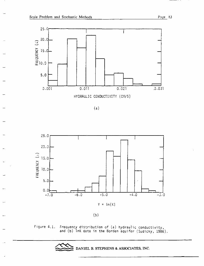
Scale Problem and Stochastic Methods P;:Lve 83
25.
2fl
-'15.C
LU
LUj
a:10. 0
5.0
0.001 0.011 0.021 .0.031
HYDRAULIC CONDUCTIVITY (CIl/S)
(a)
25.0
LU
LU
-3.0
Y = ln(K)
(b)
Figure 4.1. Frequency distribution of (a) hydraulic conductivity,and (b) inK data in the Borden aquifer (Sudicky, 1986).
DANIEL B. STEPHENS & ASSOCIATES, INC.
Scale Problem and Stochastic Methods Paste 84
possible hydraulic conductivity values is called a frequency or probability distribution
of the hydraulic conductivity of the aquifer. Based on this conceptualization, the
hydraulic conductivity value depends on probability or chance. Namely, it is not
completely predictable: only proabilities can be associated with the possible values
and hence the values are considered as realizations of a random variable. The
frequency distribution determines the likelihood (or probability) that a specific
hydraulic conductivity value will be found at a particular location.
Frequency distributions of most hydrologic properties of an aquifer generally
are taken to be either normal or lognormal. A normal distribution is characterized
by a symmetric bell shape. Lognormality implies that the distribution of the
logarithms of a random variable has a normal distribution (Figure 4.lb). However,
the distribution of a log-normal random variable itself is positively skewed (Figure
4.1 a). Many field data have shown that the distribution of porosity data in a given
aquifer is usually normal (Law, 1944 and Bennion and Griffiths, 1966), altough recent
work by Hoeksema and Kitanidis (1985) suggests that the storage coefficient may be
log normally distributed. Hydraulic conductivity data are usually reported to be
approximately lognormal (Law, 1944; Bulness, 1946; Warren et al., 1961; Bennion and
Griffiths, 1966; Ilyin, 1971; Bakr, 1976, and Freeze, 1975), as are transmissivity
values (Delhomme, 1979; and Hoeksema and Kitanidis, 1985). There are exceptions
however, as shown by Jensen et al., (1987). Figure 4.1 shows a skewed distribution
of hydraulic conductivity values in a sandy aquifer and a more normal distribution
of natural log of the hydraulic conductivity values, InK.
Inasmuch as different aquifers are formed by different geologic processes,
the distributions of hydrologic properties of different aquifers are likely to be
different. To characterize the distribution one generally uses statistical moments of
the random variable. The first moment refers to its mean. the second moment to the
variance (the spread of the distribution) and the third moment to the skewness (a
_____ DANIEL B. STEPHENS & ASSOCIATES, INC.
Scale Problem and Stochastic Methods Page 85
measure of its symmetry). Figure 4.2 schematically illustrates distributions of the
logarithms of hydraulic conductivity values in a sandstone and a shale unit.
Although the hydraulic conductivity distribution of the two geologic materials is
lognormal, the mean hydraulic conductivity value of the sandstone unit is larger than
the shale unit and the variance is larger in the shale than in the sandstone.
The application of the random variable concept to hydraulic conductivity
values seems to be valid only if no actual measurement of the parameter value is
available. However, it is suitable for analysis of uncertainty in hydrologic property
values. Even if one can determine hydrologic property values at every point in an
aquifer. due to spatial variability of the property it is still appropriate to consider the
hydraulic conductivity value as a random variable at the location. That is to say,
the value represents only one of many possible geological materials that may have
been deposited at a given point when the geological environment was created. This
random variable concept can certainly be applied to other sample locations. Thus.
hydraulic conductivity values of an aquifer may be considered as a collection of
many random variables in space. This infinite sequence of random variables is
generally referred to as a stochastic process (or a random process, random field or
random function).
For example, the set of hydraulic conductivities along a transect can be
considered as one possible outcome of a stochastic process. In a stochastic process
the value of the quantity, say conductivity, K(x), is a random variable for each
location x. Namely, if conductivity is observed at locations xl, x2 ,... .xn, the K(x1 ) is
a random variable, K(x2) another random variable, and so on out to K(xn). Each has
a probability distribution and furthermore the probability distributions may be
interrelated. The chance of finding a particular sequence of hydraulic conductivity
values along the transect depends not only on the probability distribution of the
hydraulic conductivity at one location but also on those at other locations. This
________ DANIEL B. STEPHENS & ASSOCIATES, INC.

Scale Problem and Stochastic Methods Page 86
_ SA[IDSTOIrEL U
Li
LU ~ SiL
lnK
Figure 4.2. Frequency distributions of the hydraulic conductivity valuesof a sandstone and a shale unit.
~~~ DANIEL B. STEPHENS & ASSOCIATES, INC.

Scale Problem and Stochastic Methods Page S7
implies that actual hydraulic conductivity values, along the transect are one possible
sequence of K(x) out of all the possible sequences. In the vocabulary of stochastic
processes, all these possible sequences are called an ensemble, and a realization refers
to one of the possible sequences (Figure 4.3).
In order to determine the probability of occurrence of a particular sequence
of random variables, a joint distribution of these random variables must be known.
The joint distribution is completely defined only if the probabilities associated with
all possible sequences of K(x1) values along the transect are known. Similar to the
distribution of a single random variable, the joint distribution of random variables is
also characterized by its moments. However, this joint distribution is seldom known
in real-life situations because hydraulic conductivity values sampled along a transect.
for instance, represent only one realization out of the ensemble of the hydraulic
conductivity values along the transect. Therefore, one must usually resort to
simplifying assumptions, namely, stationarity and ergodicity.
Stationarity (or strict stationarity) implies that any statistical property (joint
distribution, mean and variance) of a stochastic process remains stationary or constant
in space. Ergodicity means that by observing the spatial variation of a single
realization of a stochastic process, it is possible to determine the statistical property
of the process for all realizations (De Marsily. 1986). Since in reality one always
deals with a specific geologic formation (one realization) rather than an ensemble of
such formations, one has no choice but to adopt the assumption of ergodicity as a
working hypothesis for the stochastic approach.
Because it is difficult to obtain all of the joint distributional information
required and because in many cases important properties are assessed by moments
like the mean, variance or other lower order moments, an assumption of weak or
second order stationarity is often invoked. The first moment (mean) of K(x) is
defined as:
~ DANIEL B. STEPHENS & ASSOCIATES, INC.
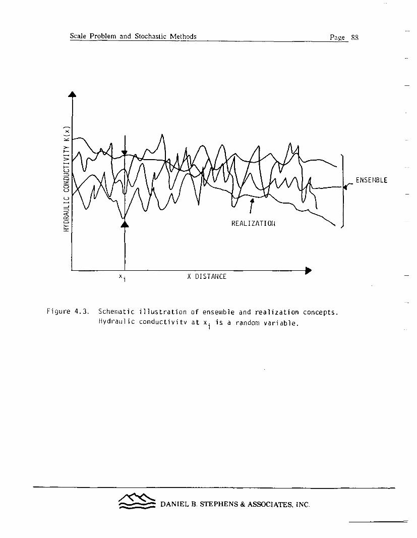
Scale Problem and Stochastic Methods P aue RRScale Problem~~ an StchatcMtosP, v v
F--
C-D
QL)
C-,
ENSEUBLEC,
REALIZATIO1I
x; iX DISTANCE
Figure 4.3. Scheiilatic illustrationHydraulic conductivity
ofat
ensemble and realization concepts.
x; is a random variable.1
DANIEL B. STEPHENS & ASSOCIATES, INC.

Scale Problem and Stochastic Methods Pai e S9
g = E[K] = { K f(K) dK (4.1.1)
where E[ ] stands for the expected value, and f(K) is the joint density distribution of
K. This means that the expected value of a stochastic process is its probabilistic
average (or ensemble average). The second moment (autocovariance or covariance
function) is then defined as:
c(Q)=cov [K(x+(), K(x)] = E[ (K(x+()-,L)(K(x)-#) ] (4.1.2)
The second-order stationarity assumptions are that (i) u = E[K] is constant, and
cov[K(x+{), K(x)] only depends on (, (i.e., c(() = cov[K(x+(),K(x)]) where ( is called the
separation distance. If the separation distance is set to zero, the covariance function
becomes the variance, 02 . An autocorrelation function is simply defined as the ratio
of covariance function to its variance, i.e.:
p = c() (4.1.3)0.2
Values of the autocorrelation function are always in the range between -I and 1.
The autocorrelation function represents the persistence of the value of a property in
space.
To explain the idea of the autocorrelation function, we will consider two
identical sine waves, w(x)=sinx, except they are separated by a distance E as shown
in Figure 4.4a. Note that the sine waves are strictly deterministic functions. If a
correlation coefficient, r, between these two waves is calculated, by regression
DANIEL B. STEPHENS & ASSOCIATES, INC.
Scale Problem and Stochastic Methods Par-e 90Scale Problem and Stochastic Methods Page 90
+1
0
- 1
(a)
01
-1
+1
W(x+:;) (b)
r=1
r=0.7 0 r=0x
-1W (x+,:-)
:) (d)
+1I +1
0
- 1
+1r = -1
(C.
0
-1 -1W(x+,)
W(x+,)(e) (f) (9)
Figure 4.4. Diagrams to illustratelation function.
the concept of an autororre-
DANIEL B. STEPHENS & ASSOCIATES, INC.

Scale Problem and Stochastic Methods Page 91
analysis, r has to be I if ( = 0; if w(x) is plotted against %k'(x+j) at ( = 0, all the
points will lie on a 45 degree line since they are identical (Figure 4.41). As one of
the waves is shifted by a distance E#AO, the plot of w(x) vs. w(x+() will start to
scatter around the diagonal line as shown in Figure 4.4c. The correlation becomes
less than unity because the values of the waves no longer correspond at every
distance. As the wave moves out of phase exactly by one half of a wavelength, the
scattering become even more significant and the correlation drops to zero (Figure
4.4d). This zero correlation indicates that the points of the two waves at this
separation distance are completely different. Figure 4.4e shows that a further
increase of the separation distance will reduce the scattering but the correlation
becomes negative. As the separation distance approaches one half wavelength, i.e.,
the trough of one wave matches the peak of the other, and the correlation drops to
-I (Figure 4.4f). This r = -I value implies that these two waves are identical but in
an opposite manner. If one plots the r values at each separation distance vs. the
separation distance, one obtains a plot of an autocorrelation function (Figure 4.4g).
Therefore, the autocorrelation function is a measure of the similarity of the series at
different separation distances.
Generally, the autocorrelation function of hydraulic conductivity data tends
to drop rapidly as the separation distance increases. The decline of the correlation
may be represented by many different autocorrelation models. The one commonly
used is an exponential decay model (Bakr et al., 1978; Gutjahr et al., 1978, Gelhar et
al., 1979, Yeh et al., 1985a, b, c):
p(W) = expL-.] (4.1.4)
where p(() is the correlation function, ( is the separation distance, and X is the
_______ DANIEL B. STEPHENS & ASSOCIATES, INC.
Scale Problem and Stochastic Methods Page 92
correlation scale. The correlation scale is a characteristic length beyond which the
correlation between data is no longer considered significant. However, this definition
is rather arbitrary and an integral scale is often used instead. The integral scale is
defined as the area under a autocorrelation function if the area is a positive and
nonzero value (Lumley and Panofsky, 1964). For the exponential model (equation
4.1.4), the integral scale is a separation distance at which the correlation drops to the
exp(-l) level. At this level, the correlation between data is considered insignificant.
That is, the data points separated by distances larger than the correlation scale are
only weakly associated with each other.
On an intuitive basis, the correlation scale may be interpreted as the average
length of clay lenses or sedimentary structures. Hydraulic property values of the
samples taken within the clay lens tend to be similar; correlation between sample
v\alues is near unity. However, sample values are quite different if one sample is
taken within the clay lens and the other outside the lens; the resulting correlation
will be small. Thus, the autocorrelation function is a statistical measure of the
spatial structure of hydrologic parameters. Table I presents a summary of
correlation scales for hydraulic conductivity or transmissivity in a variety of geologic
environments in which data were collected by methods ranging from cores to
pumping tests. We must point out that there has been very little published research
to confirm the geologic significance of the correlation length (Byers and Stephens.
1983; MacMillan and Gutjahr. 1986).
For the sake of simplicity. the above discussion on autocorrelation function is
restricted to one-dimensional data (i.e., data collected along a transect). The concept
can be applied to a two- or three-dimensional data set as well. For example, a
commonly used three-dimensional exponential autocorrelation function in groundwater
hydrology is:
_______ DANIEL B. STEPHENS & ASSOCIATES, INC.

Scale Problem and Stochastic Methods Paee 93I, _
Table 1 JVariances and correlation scales for log hydraulicconouctivity or log trans-nissivity (Gelhar, 1986).
Ca2rrriaggon overmlSourc: Mvedium Scm -I S-zue. rn
Baoir E 1976] iandstune aquiier 0.3-i0 V 100SM1111 C 197,31 oulwasli sand 0.3 0.4 V 'Driliuirnme r 1979] limeszonc aquifer .3 6300 H ~ .0ainsarua cc9801 basin ,ill augutier 1.0 300 H .. 0.Auswo un 3ressier Hamm~ Rcu. Medii. 0.4-I1 14-;9 4 ~ 00
Lr I98 I] :e-rancan sotiL;.gxynuare ef .2g. gwea~nr ~fnaIc 0.S <: H (
'i98l] ~~~~suosoiiSiso na Wie-rrniya AiD, z:ay ;oam 0.0 0. HL19811, ;oij tagluvias)
V~era ef jig. Yoio 50od 0.9 IS R M07:9X11 iailuvial f~nl
£hergrv andj Doctor aiIU%'Iag aQU~ife 0.3 sKo H oo198:] itiooa pmvcis)
3veri and 5Sephens luiaig~ sana 0.9 0.1 iV 5£ 193(31 >4R .
Horksiema gnj Sandstone~ zoulfer 0.6 45.000 H S 10'.<iroaniais C L9SS]'
Hws.7,ingtgi ri9sS] sand and 3ravet 1.9 0.;5 Vsw&J;cK% -'985] .)utgasn iunflU 0.o 0.1V
Cirrewiggon icuws basca on e- z ~rrcIaggOM disl3nce: i-{. loanzongai sampling. V. vertic=1 sarnognng.
DANIEL B. STEPHENS & ASSOCIATES, INC.
Scale Problem and Stochastic Methods Page 94A
IF -1/21P(O ) = exp1_L( I/yj)2 + (E2/X2) + (,/\3)2 F (I.1a)
where t is the separation distance, and 41, 42, and 43 are separation distances in x, y,
z directions, respectively. Integral scales in the x, y, and z directions are X. X2, and
X3, respectively. If the integral scales are the same in all directions, then the
stochastic process is called a statistically isotropic process. If these values are
different, then it is called a statistically anisotropic process. Note that statistical
isotropy and anisotropy are different from hydraulic conductivity anisotropy in
classical hydrology. Statistical anisotropy simply implies that the hydrologic property
(such as hydraulic conductivity) of an aquifer is correlated for a longer distance in
one direction than in other two directions. For instance, in a perfectly stratified
aquifer (e.g. laterally continuous "layer cake" sedimentary sequence), correlation scales
in the horizontal directions are likely to be the same, but they will be much longer
than the correlation scale in the vertical direction. This is due to the fact that
within each layer, the material is considered to be effectively homogeneous. A short
vertical correlation scale reflects a rapid lithologic change in the vertical direction.
In Figures 4.5a and b, statistically isotropic and anisotropic aquifers are schematically
illustrated. Figure 4.5c depicts an ellipsoid formed by anisotropic correlation scales.
Hydrologic property values within the ellipsoid are considered correlated or similar.
and those outside the ellipsoid are uncorrelated or dissimilar. A three-dimensional
correlation function generally represents more closely the average physical dimensions
of sediment bodies (such as clay lenses) than the one-dimensional correlation function.
If a stochastic process (e.g. hydraulic conductivity) has a constant mean we
refer to the process as having no drift; that is, the first statistical moment is constant
over distance. If a process exhibits no drift and its autocorrelation function depends
_ __ DANIEL B. STEPHENS & ASSOCIATES, INC.

Scale Problem and Stochastic Methods Pag~e 95Scale Problem and Stochastic Methods Page 95~~
A1-A 2-\ 3
(a) Statistically isotropic aquifer and a sphere formed by anisotropic covariance function.
_1- -. ., _ = .' 3 ;-.
lt, ..
Cr yc
° °S O~ ~~~~a° 00 Ca
(b) Statistically anisotrooic aquifer
(c) An ellipsoid formed by athree-dimensional anisotroDiccovariance func:ion.
'I X '2 a A
,igure I.5. Schematic diagrams illustrating stochastic zonceots inground-water hydrology.
-- ""~ DANIEL B. STEPHENS & ASSOCIATES, INC.

Scale Problem and Stochastic Methods Page 96
on the separation distance only, the process is considered as a second-order stationarv
(or statistically homogeneous) process. If the spatial distribution of hydrologic data is
second-order stationary, one is then able to use the first moment and its covariance
function to characterize its spatial variability. On the other hand. data that do not
fit the definition of the second-order stationarity process are considered as non-
stationary processes. A non-stationary process describes data which has a definite
trend in space (i.e., the mean varies with distance or the covariance depends not just
on the separation distance). For example, in a sedimentary basin a formation may
have facies changes which cause hydraulic conductivity to decrease gradually toward
the center of the basin. However. for many cases the data with a trend may still be
treated as a stationary process after the trend is removed.
Figure 4.6 schematically illustrates the meanings of stochastic terms discussed
above. In Figure 4.6a, a regular sine wave and its autocorrelation function are
shown. Figure 4.6b shows a signal created by a random number generator. The
autocorrelation function drops rapidly from +1.0 at 0 separation distance, then
fluctuates slightly about 0. This type of behavior indicates that the signal is
uncorrelated or statistically independent from one point to the next. Both of these
series are stationary: that is, no significant trend exists in the data, and the
covariance presumably only depends on the separation distance. A non-stationary
signal is shown in Figure 4.6c, where the data increase steadily in value along the
sequence. The autocorrelation function shows steadily decreasing correlation. Figure
4.6d shows a combination of Figures 4.6a and b, a sine wave with superimposed
noise (uncorrelated signal). Perfect autocorrelation does not occur except at 0
separation distance, but the periodic component of the series is revealed by the
second peak in the autocorrelation function. Figure 4.6e is a combination of Figures
4.6a, b. and c, a sine wave combined with a linear trend with superimposed noise.
Due to the existence of the trend. the series is non-stationary. Note that the trend
-_______ DANIEL B. STEPHENS & ASSOCIATES, INC.
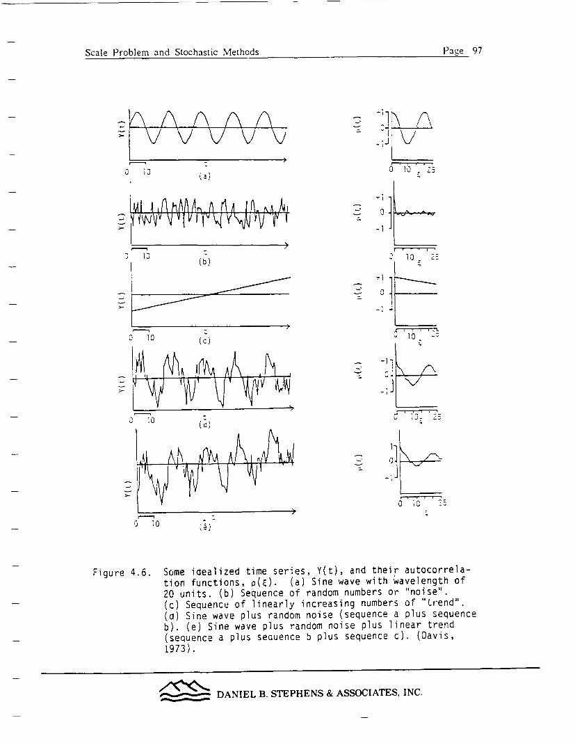
Scale Problem and Stochastic Methods Scale Problem andStochasticMethodsPage 97
V V V V �)- 'in
<JI~~~~~~~~~
0 1 0 - 200 10(a)
ml f nhAAi1AM. (A ~ A P J 4II
0
-1I-
-
\IJ\j~yV WIV II'V ~Y 4 V\ Wv -~I
70 10IU Q,
t(b)
-I
0
-1
0 10 (C)
I10 (a)
.�] � N. am A I, aI ,I I I I T
�p
0.
I I C
Figure 4.6. Some idealized time series, Y(t), and their autocorrela-tion functions, p(E). (a) Sine wave with wavelength of20 units. (b) Sequence of random numbers or "noise".(c) Sequence of linearly increasing numbers of "Lrend".(d) Sine wave plus random noise (sequence a plus sequenceb). (e) Sine wave plus random noise plus linear trend(sequence a plus sequence b plus sequence c). (Davis,1973).
w DANIEL B. STEPHENS & ASSOCIATES, INC.

Scale Problem and Stochastic Methods Page 98
further reduces our ability to discern the periodic component in the series.
Using the stochastic concept, many field data have been collected and
analyzed in the past decade. One typical example is the analysis of hydraulic
conductivity data in the Borden sandy aquifer, collected by Sudicky (1986). Thirty-
two core samples were taken from cross-sections of two perpendicular transects.
Each core sample was cut into subsamples of 0.05m in length. A total of 1279
hydraulic conductivity measurements were made from these small samples. Figures
4.7 and 4.8 offer a view of the spatial variability of hydraulic conductivity in the
aquifer. The results suggest that the Borden aquifer is heterogeneous over the
distance that the measurements were performed with the local hydraulic conductivity
field having a complex, lenticular structure. Several very distinct but thin lenses of
low hydraulic conductivity are clearly visible in the profiles. A stochastic
characterization of the spatial variability was carried out. The variance of InK (the
natural logarithms of K) was found to be 0.38. which included the variance due to
uncorrelated variations below the scale of measurement (nugget effect, Section 4.2).
Autocorrelation functions of the two cross-sections in the horizontal and vertical
directions are illustrated in Figure 4.9 a.b.c and d. Using equation (4.1.5), Sudicky
(1986) found that the autocorrelation function of InK is anisotropic with X, = X2 = 2.8
and X3 = 0.12 m, in horizontal and vertical directions, respectively.
4.2 Geostatistics
As mentioned in Section 4.1. there are two approaches to deal with aquifer
heterogeneities: (1) the effective hydrologic property approach, and (2) estimation of
property values at unsampled locations. The first approach will be explored in the
later section dealing with spectral analysis. Here we will discuss some basic concepts
and tools for the second approach. Detailed discussions can be found in textbooks by
Journel and Huijbergts (1978) or De Marsily (1986).
_______ DANIEL B. STEPHENS & ASSOCIATES, INC.

IIII I I I I I I I I I I II I
U
2:mr,tzCnmItxm�4CnRo
Cn6n
mCn
�4n
-J
Uj
2I9. 145
21a. 19S
211. IGs
211. 395
211. IIs
211. 195
217. 64S
217. 335
4 0~-
-~~~~~~~~~ C - ~ ~ ~ ~ ~ ~ ~ ~ ~
n-1
(A
0
(b
laeI0
(9
0
0 I 2 3 4 5 6 7 a 9 t I 0 ?1 1 3 1 4
LONGITUDINAlL 0151fhlCE [MIiI S 1 6 1 7 1 a
I-I 9
Figure 4.7. Cross-sectional view of the hydraulic conductivity distribution along a longitudinaldirection in the Borden sandy aquifer (Sudicky, 1986).
-v
(D
o0'.0
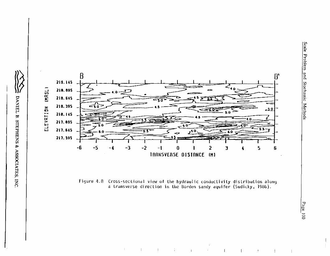
0
a~~~LI 0mLaA r210. 645
~~~~in 4 .03scn Z
a 1 1: 218. a45 4.5
m > ~~~217. 395 2oo
>:~~~~217. 3ss_95I
-6 -5 -4 -3 -2 -I 0 1 2 3 4 5 6
Cl) IDANSVEnSE DISTANCE (1I)
Figure 4.8 Cross-sectional view of the hydraulic conductivity distribution alonga transverse direction in the Borden sandy aquifer (Sudicky, 1986).
(D

I I I I I I I I I I I I I
1.02~:C)
-Chi
C-)C)I-
I I I I I I I- a) - l
- I I I- I
Estimated longitudinal
nexp (-t3/A 3 ), n= 0.75, -
0.0
2CCD
I,1-j
-C(4
C)C-)CD
¢m
CiMm~T1IVxMIR°
M
zn
C/)(A
(D
0a-
p
n
I
0
0.-
(A2
A3= 0.12iiiI I I I i
0.0 . . . . . . .0.1 0.2 0.3 0.4 0.5 0
VERTICAL DISTANCE (mii)HOKIZONIAL SCPAPAIION D)ISTANCE (,m)
1.0 1.0
CD
1-
,-J<CIw(4
C)1--
0.0
I I I I I I I I
I I I I II
- C[stimated transverse-* nexp(-k /A )., ii=0. 75
- A3 =0. 12111A I * I , I I I , _
I I I I'2:C)
1-.-<C
a
11
CD
C):D
0 t 0
I I I
0.0
I1 n
I I I
- Estimiiated transverse* ~nexp)(-E 2/A2 ) . n=0.75,
A = 2. 8 InI I , i * I I_-i
10.()-1.O 0t n n s
U U. I 0.2 0.3 0.4 0.5- .U . . . .
_ _
0.0 2.0 4.0 6.0 8.0VE Rt I CAL I S] ANCE (m)
1101ItONI[AL SPAPRAHrN 5I)SIAHLCE (m)
FiuLJre 4.9. Vertical and horizontal autocorrelation functions for lnK along cross-sections in Hielongitudinal and transverse directions. n represents the ratio of the true variance(lotal variance milnus the nulqet effect) to the total variance.
p
m
3(tC)
Scale Problem and Stochastic Methods Pi,:le 102
Geostatistics is basically a statistical method to estimate or interpolate the
parameter values at points in space where no samples are available. The technique
has been widely used for decades in the mining industry to estimate ore grades
(Journel and Huijbergts, 1978). Recently, the technique has been applied to
groundwater hydrology to deal with spatial variability problems. In principle,
geostatistics concepts are similar to the stochastic concepts. They both are used to
deal with variables distributed in space. However, some of the terminology is
different. For example, the term "random function" is used in geostatistics to
defined a collection of correlated random variables. That is, at a point xl, the
function, F(xl) is a random variable and the random variables at xl and x2+( are not
independent but correlated. From this definition, it is clear that the random function
is equivalent to the stochastic process defined earlier. Similarly, a "regionalized
variable" is used in geostatistics to define a function f(x) which takes a value at
every point x of coordinates (xI, x2, X3) in three-dimensional space (Journel and
Huijbregts, 1978). A regionalized variable is simply a particular realization of a
certain random function or stochastic process. We will point out some other
differences in the following text.
Two important parts of geostatistics are (1) identification of the spatial
structure of the variable (variogram estimation, trend estimation, etc.) and (2)
interpolation or estimating the value of a spatially distributed variable from
neighboring values taking into account the spatial structure of the variable (kriging,
co-kriging, etc.. Davis, 1973).
Similar to the autocorrelation function described previously, the variogram
is simply a way of defining the spatial structure of a random field. Variogram
analysis is based on the intrinsic hypothesis which is less stringent than the second-
order stationarity assumption. Recall that second-order stationarity requires that the
data have a constant mean and the covariance function depends on the separation
_______ DANIEL B. STEPHENS & ASSOCIATES, INC.

Scale Problem and Stochastic Methods Pace 103
distance only. However, the intrinsic hypothesis requires only that the mean of the
differences of the data values is constant, and the variance of the difference of data
values depends on the separation distance, i.e. [K(x+() - K(x)] satisfies:
E[K(x+() - K(x)] = m (4.2.1)
2 var[K(x+() - K(x)] - y(y) (4.2.2)
where K(x's are regionalized variables, and y is a function of i. and not of x. y(Y)
is called the variogram, sometimes also called semivariogram. Figure 4.10 shows the
general behavior of a variogram. As indicated in the figure, when the variance of
the variable is finite, the variogram tends towards an asymptotic value equal to this
variance, var[K(x)]. This is called the sill of the variogram, and the distance at
which the variogram reaches its asymptotic value is called the range, X. The range
is analogous to the correlation scale discussed earlier: beyond the range, the
regionalized variables K(x) and K(x+E) are no longer correlated. In fact, the
variogram is a mirror image of the covariance function if the data is a second-order
stationary process.
The main types of variograms commonly used to fit sample variograms
(variograms estimated from field data) are: linear, spherical, exponential, Gaussian,
and cubic. Figure 4.11 shows the shapes and equations of these variograms.
Generally, a linear variogram, as shown in Figure 4.11a, suggests that the process has
an infinite variance and that there is no covariance function. i.e., it is not a second-
order stationary process. In this case, one has to rely on the intrinsic hypothesis to
analyze the data. Theoretically, all variogram plots pass through the origin; the
variogram is zero at a separation distance of zero. However, variograrns obtained
______ ,DANIEL B. STEPHENS & ASSOCIATES, INC.

Scale Problem and Stochastic Methods Page 104iScale Problem and Stochastic Methods Pace 104
RANGE
L-)
Z4J<F
MX
Figure 4.10.
SILL
'11� "/111� C(0) =Cov. fn.
SEPARATION DISTANCE
General behavior of a variogram.
-_____ DANIEL B. STEPHENS & ASSOCIATES, INC.

Scale Problem and Stochastic Methods Paae 105
a II
7
2 -
I ft'I - -- - 7 I-
0 2*/S ahI
0 Ala model in A' Wh* A < 2
(bi sphencal modelw[3 (h) _ I (h)]
; '_ i -- a a
A<a
_ _
t 05-
(cl cxponential model
(dl Gaussian model
[cl cubic model
1.1 h >a
W(l - elp( -h"3]
W II - eop( --4:all']
- s,5 + -5- 07
3 .1 a ,a4 <
30If) hiting on a -linear plus sphencalr model esirn~ipel
< a
2
, C i_____ ____ , 13 3 h 4 613; I3)-- (-
/- 13.34 (1
05/ I 8000
600 -.- -- - - - - - - -
0 o/2 a 0 051015 20 30 40
Figure 4.11. A diagramii showing the shapes and equations of various variograms(de MIarsily, 1986).
4 J< 1 5
0-i~ ..... DANIEL B. STEPHENS & ASSOCIATES, INC.

Scale Problem and Stochastic Methods Pa< e 106
from field data often exhibit a jump at the origin. as shown in Figure 4.12. This
apparent jump is called the nugget effect and represents the uncorrelated subscale
variability or measurement errors. The variogram can be either isotropic or
anisotropic as in the covariance function. It is also likely that there are multiple
correlation scales that appear when testing over different scales. ranging from
laboratory to field to required scale. Figure 4.13, (Gelhar, 1986).
The other part of geostatistics is Kriging. The most general form of Kriging
is termed "Universal Kriging," in which the values of points may be estimated from
irregularly distributed samples in the presence of trends (or nonstationarity). If the
data set is stationary, a less involved operation can be used to estimate the values of
points. This technique is referred to simply as "Ordinary Kriging" or "Kriging" (see
Bras and Rodriguez-lturbe, 1985. and Journel and Huijbregts, 1978).
A common application of Kriging in groundwater hydrology is the estimation
of hydraulic conductivity or transmissivity values at unsampled locations in between
test wells (see Delhomme, 1979). For example, in an attempt to use a two-
dimensional, finite difference, groundwater flow model to simulate flow fields in a
groundwater basin, one may design a 2000 node mesh for the entire basin. However,
only 50 measured transmissivity values scattered around the entire basin may be
available. To objectively assign transmissivity values to the remaining nodes, one
may have to resort to use of mathematical tools. Kriging is one of the possible tools.
To find the hydraulic conductivity estimate K' of the unknown quantity K0,
Kriging uses a weighted sum of all the available sample values (measured hydraulic
conductivity values):
nKS XiK 1 (4.2.3)
i=I
____ DANIEL B. STEPHENS & ASSOCIATES, INC.
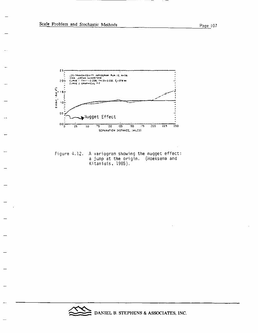
Scale Problem and Stochastic Methods P ns 1)7I -�' IV,
-.'-TftNSWt$S1V~ry 1,A0IQGRAM RUN~ 12. F4.3
: o-4 .CRCAN w.NOs-O'sC20U" C'.AvE I ?''I:C 209. TN431.O332. 1, sZTWM
- 'JQVC Z GRAP'C.;L rnT
_- 1 5,r
- 10o
05Nugget Effect
00-0 25 _0 'S 'CC
I
-4JI
L - -- -- .....
125 :50 :75 Z 00 225 2 50
DISTANCr- ;IAR-ESSEPARATION;
Figure 4.12. A variogram showing the nugget effect:a jump at the origin. (Hoeksema andKitanidis, 1985).
DANIEL B. STEPHENS & ASSOCIATES, INC.

Scale Problem and Stochastic Methods Pagze 108Scale Problem and Stochastic Methods Pa�ze 108
INTERBASINAQUIFER
ALLUVIALAQUIFER
FLUVIALAQUIFER ?
CORE
mm m kmSEPARATION DISTANCE r
earth
Figure 4.13. Hypothetical InK variogram illustrating the notion of scale-dependent correlation scales (Gelhar, 1986).
_______ DANIEL B. STEPHENS & ASSOCIATES, INC.

Scale Problem and Stochastic Methods Pace 109
where Xi are the weighting factors, and K; are sample values. In order to limit the
choice of the weighting factors, we will impose two conditions. The first condition
is that the expected value of the estimate of K should be the same as the expected
value of K, i.e.,
E[ K]= E [ K] (4.2.4)
It follows that in the constant mean case the sum of the weighting factors has to be
unity.
n
Z Xi = 1 (4l.'.5)i= 1
The second condition is that the error of estimation should be minimal:
E[ (K' - K)2 = = minimum (4.2.6)
This latter condition, along with 4.2.5 leads to a system of equations of the form:
nZ Xj Y(Xi - xj) + A = Y( Xi - x0 ) (4.2.7)
j=o1
where y(x1 -x; ) represents the variogram corresponding to a separation distance (
equal to the distance between points xi and x;. Similarly, y(x1 - x0 ) represents the
variogram over a distance equal to that between the point to be estimated and the
point x;. jp is a Lagrange multiplier. Combining the constraint that the weighting
DANIEL B. STEPHENS & ASSOCIATES, INC.
Scale Problem and Stochastic Methods Paize 110
coefficients must sum to one. the system of equations can be solved to obtain optinmal
Xi values which can then be input to equation (41.2.3) to obtain the estimate of K
The estimator, K' is a linear combination of the n data values (4.2.3). The n weights
Xi are calculated to ensure that the estimator is unbiased and that the estimation
variance is minimal. Kriging is a best linear unbiased estimator (BLUE).
The Kriged estimate Kg is based on samples located a distance away from
the estimated point. The values at these distant points are only partially related to
the value at the Kriged point, the degree of relationship being expressed by the
variogram. Therefore, we do not expect our estimate, K', to be exact. The
inexactitude of the estimate is the Kriging variance, rK, which is:
n
oK (x0) = XE j -Y(X - xO) + Ai (4.2.8)
j= I
The smaller the variance, the greater the reliability of the estimate K' . Conversely,
an estimate with a large associated variance must be utilized with caution. One can
also use the Kriging variance in determining the optional location for additional field
tests. For example, hypothetical locations can be added to the actual data base to
calculate the reduction in the Kriging variance. Thus, Kriging could be a valuable
tool in quantifying uncertainty in interpolated data and in assessing the value of
additional data during site characterization.
Kriging is different from other interpolation or extrapolation techniques
because it considers the spatial structure (variogram) of the variable. It also provides
a measure of the probable error associated with estimates of the unknown values.
However, for many cases, Kriging may have no advantages over polynomial trend
surface and may even perform poorly by comparison (Davis, 1973). Unlike some
_______ DANIEL B. STEPHENS & ASSOCIATES, INC.
Scale Problem and Stochastic Methods Page III
regression models that fit a surface to the data base, Kriging preserves the values at
points of measurement. Note that the model and objections behind polynomial or
surface fitting differ from those in kriging. For that reason a comparison bet\s een
them may not be appropriate. In trend surfaces the objective is to fit the mean
value while in kriging reconstructing the actual surface is the goal in this sense
kriging includes a kind of conditioning.
Kriging can also be used in conjunction with numerical simulations that may
be useful in calculating ground water travel time. In a numerical model the aquifer
is discretized into grids, within which hydraulic properties are assumed to be
uniform. However measurements of transmissivity or hydraulic conductivity, for
example, represent a much smaller scale than the grid blocks of the model. In
contrast to ordinary Kriging described previously in this section, block Kriging can be
used to obtain average properties for the grid block (De Marsily, 1986). That is, the
spatial correlation structure obtained from local measurements can be used to
interpolate on an point or area basis. De Marsily et al. (1984) describes a method of
identifying hydraulic characteristics of a reservoir from aquifer pumping tests which
combines Kriging and numerical simulation. The approach allows one to utilize a
variety of available hydrogeologic information at different scales. Kriging has also
been used by Devary and Doctor (1982) to estimate uncertainties in pore velocity at
the Hanford site from estimated fields of hydraulic conductivity, effective porosity.
and hydraulic conductivity. A similar approach to estimate pore velocity is described
by Neuman (1984).
In most field problems, groundwater hydrologists are likely to have both
transmissivity and hydraulic head, or the specific capacity data. Hydraulic head and
specific capacity are generally correlated with transmissivity. It may be desirable to
estimate transmissivity values at unsampled locations, using both measured
transmissivity and hydraulic head values or specific capacity data, instead of using
DANIEL B. STEPHENS & ASSOCIATES, INC.

Scale Problem and Stochastic Methods Page 112
transmissivity only. This type of technique using the Kriging concept is called co-
Kriging. Detailed discussion on this subject is available in De Mlarsily (19S6).
Gutjahr (1981), and Kitanidis and Vomvoris (1983). Neuman (1984). Willianms (1987),
and Hoeksema and Kitanidis (1984) applied this approach to groundwater flow
simulations.
_______ DANIEL B. STEPHENS & ASSOCIATES, INC.

Scale Problem and Stochastic Methods Page 113
4.3 Stochastic Analysis of Spatial Variability
The statistical description of spatial variability of hydraulic properties of
subsurface materials has led many researchers to investigate the effect of randomly
distributed parameters on the governing equations. The model used to investigate this
type of problem is generally called a stochastic model. Although stochastic and
deterministic models use the same governing flow and transport equations for porous
media, the former differs from the latter in that its input functions are uncertain
and, therefore, the model output must be described in probabilistic rather than
deterministic terms (Neuman, 1982).
For example, a deterministic, three-dimensional, groundwater flow model
requires values of hydraulic conductivity and storativity at every point in three-
dimensional space, if we assume that the initial and boundary conditions and sink
and source terms are prescribed. The output from the deterministic model is a
realization of hydraulic head values corresponding to those parameters at each point
in space. However, in a stochastic model, the hydraulic conductivity and storativity
are considered as stochastic processes in space which are described in terms of
means, covariances, and other statistical terms, instead of a value at each point. The
output consists of many possible head distributions that relate to the input
parameters. Therefore, the head is a stochastic process which can be described in
terms of statistical parameters such as mean, variance, covariance, etc. In other
words, the stochastic model produces a probabilistic result which can be utilized to
assess the uncertainty in predictions due to heterogeneity of aquifer properties.
In the past few decades, many researchers in groundwater hydrology have
applied stochastic models to study flow and transport through heterogeneous porous
media. The following is a summary of these works which include Monte Carlo
simulation, conditional simulation, spectral analysis, and fractal analysis.
_______ DANIEL B. STEPHENS & ASSOCIATES, INC.

Scale Problem and Stochastic Methods Pave 114
4.3.1 Monte Carlo Simulation. The most intuitive approach to dealing \with
spatial variability in a stochastic sense is called Monte Carlo simulation. It is a very
powerful method, since fewer assumptions are required than in all of the other
stochastic methods. However, it may require extensive computer time and a careful
analysis of the results. The principle of the method is rather simple. The method
assumes that the probability distribution of the variable (for example, hydraulic
conductivity) and its covariance function are known from measured field data. Then,
many possible realizations of hydraulic conductivity values that conform to the
assumed probability distribution can be generated by using a pseudorandom number
generator with special techniques (Gutjahr, 1987; Smith and Freeze, 1979; Mantoglou
and Wilson, 1982). Each realization of the parameter values is input to flow and
transport equations which are then solved by either numerical or analytical methods.
In most cases, numerical methods are used. Thus, a solution is obtained for each
realization of the input parameters. If there are N realizations of input parameters
used, there are N realizations of output from solving the governing equations. It is
then possible to statistically analyze the output for each realization to obtain expected
value, variance, covariance, and distribution. The idea is illustrated in Figure 4.14.
There are difficulties associated with the simulation method. First, a large
number of realizations is necessary in order to obtain meaningful statistics. This
implies that extensive computer CPU time is required, and this method is costly.
Second, a groundwater basin has to be discretized into many elements or blocks in
numerical simulations. Using a direct numerical solver (such as Gaussian elimination)
to solve such a large system of equations in numerical models is generally not
feasible because of memory storage limitations of computers. Often, the solution
technique has to rely on iterative methods. Iterative techniques may reduce the
memory storage problems but may not result in the convergence of the solutions to
the true ones for highly variable input parameter values. In variably saturated flow
________ DANIEL B. STEPHENS & ASSOCIATES, INC.
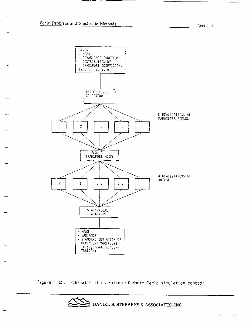
Scale Problem and Stochastic Methods.
Pace 1II
11 REALIZATIMOS CFPARAkETER FIELDS
i REALIZATIONS OFOUTPUTS
Figure '1.14. Schematic illustration of Monte Carlo simulation concept.
DANIEL B. STEPHENS & ASSOCIATES, INC.
Scale Problem and Stochastic Methods Page 116
situations or other highly nonlinear flow and transport systems. the governing
equation must be solved by iterative methods. and one is often unable to obtain a
solution even for homogeneous properties. The difficulties in obtaining solutions for
flow and transport in such nonlinear systems with stochastic parameters are
tremendous. Although these are grave difficulties. one major drawback of the
approach is that no clear relationship between the statistics of input parameters and
output parameters can be easily derived.
Applications of Monte Carlo simulations to investigate the effect of
heterogeneity on flow through porous media were first used by Warren and Price
(1961). Following their work, studies were made by Warren and Skiba (1964), Bibby
and Sunada (1971). and Heller (1972). All of these works are related to petroleum
reservoirs. The first study directly related to groundwater hydrology was carried out
by Freeze (1975). Freeze essentially extended the approach of Warren and Price
(1961) to the multivariate case in which hydraulic conductivities, compressibilities, and
porosities all vary randomly in space and are mutually correlated. The objective of
his study was to investigate the uncertainty in hydraulic head prediction due to
aquifer heterogeneity. Groundwater travel times and paths depend partially on the
hydraulic gradient distribution, which in turn is related to hydraulic head
distribution. Uncertainties in predictions of head distribution, of course. will result
in uncertainties in prediction of groundwater travel times and paths. Thus, it is
appropriate to discuss his work in detail in this section. Furthermore, discussion on
the weakness of his work may lead to a better understanding and future utilization
of Monte Carlo techniques to predict groundwater travel times and paths.
Freeze (1975) considered both steady-state flow under constant head
boundary conditions and transient consolidation of a clay layer under similar
boundary conditions and prescribed head at time zero. A one-dimensional flow
domain was discretized into many blocks. Random hydrologic parameters (log
-_______ DANIEL B. STEPHENS & ASSOCIATES, INC.

Scale Problem and Stochastic Methods Pa,-e 117
hydraulic conductivities, compressibilities, and porosities) were assigned to each block,
and these parameter values were independent from those at adjacent blocks (i.e.. no
correlation structure was considered in generating the random hydraulic parameters).
An analytical method and a numerical method were used to determine the hydraulic
head distributions for steady and unsteady flow, respectively. Solutions were then
analyzed for a given number of blocks and a given choice of statistical parameters
such as mean parameter values, variances, and correlation coefficients between
parameters.
Based on the Monte Carlo analysis, Freeze concluded that (I) there is no
simple way to define an equivalent homogeneous porous medium for transient flow in
a heterogeneous porous medium; and (2) the consideration of spatial variability of
hydraulic properties in a stochastic sense may lead to very large fluctuations in the
computed hydraulic head values. Therefore, he expressed the pessimistic view that
the prediction of hydraulic head using any deterministic model may suffer from very
large errors. He further questioned the usefulness of determining aquifer
characteristics by means of aquifer test analyses, which rely on deterministic
analytical solutions and the assumption that the aquifer is homogeneous.
Such pessimistic views on groundwater flow modeling by Freeze were
challenged by Gelhar et al. (1976). They attributed the large variance in calculated
hydraulic head in Freeze's work to the dimensionality of the model used. They
indicated that the head variance will be reduced significantly in three-dimensional
models. When a one-dimensional model is used, the flow must travel directly
through impermeable layers. The hydraulic head gradient near an impermeable layer
thus has to increase substantially to allow water to flow. In a three-dimensional
problem, water takes the least resistant route and avoids the impermeable paths.
Therefore, the head gradient is smaller than in the one-dimensional case. Head
variance in a three-dimensional model is also much smaller than in the one-
_______ DANIEL B. STEPHENS & ASSOCIATES, INC.
Scale Problem and Stochastic Methods Pi ie 118
dimensional case. Furthermore. Freeze's analysis assumed that hydrologic paranmeters
in adjacent finite difference grids were independent. but within a grid the properties
were constant. This assumption implies that the parameter values are correlated over
a block; that is. the size of the block determines the correlation scale. Bakr et al.
(1978) showed that the head variance is directly proportional to the square of the
correlation scale. Consequently, the choice of the size of the block could
significantly affect magnitude of the head variance. Therefore, Freeze's analysis was
most likely overly pessimistic.
More realistic simulations than Freeze's study on uncertainties in hydraulic
head were later conducted by Smith and Freeze (1979a and b) using a Monte Carlo
technique. Steady flow through one- and two-dimensional random hydraulic
conductivity fields was simulated using a finite element model. The hydraulic
conductivity K was assumed to be lognormally distributed. Anisotropic spatial
correlation structures (statistical anisotropic covariance function) of the random
conductivity values were incorporated by using a first-order nearest-neighbor
autoregressive model. One technical weakness of their work is that one has minimal
control on the shape of covariance function generated by the nearest-neighbor model.
In the two-dimensional analysis, a hypothetical rectangular aquifer was used in which
constant hydraulic head boundaries were imposed on two opposite sides of the
aquifer and no flow boundaries on the others.
The results of their simulations show that for the case of unidirectional
(uniform) flow, the uncertainty in hydraulic head must be interpreted in light of the
ratio of the correlation scale to length of size of the aquifer. The uncertainties in
head (represented by the standard deviations of hydraulic head distribution) increase
as the extent of the heterogeneity increases and/or as the correlation scale/length
ratios increase. A comparison of the results of one- and two-dimensional flow
regimes indicated that the standard deviation is smaller in the two-dimensional
_______ DANIEL B. STEPHENS & ASSOCIATES, INC.

Scale Problem and Stochastic Methods Page 119
problem. They also investigated the effects of nonuniform flows by rearranging the
boundary conditions of the hypothetical aquifer. The results from nonuniform flow
fields simulations led to the conclusion that the uncertainty in model predictions
depends upon both the spatial heterogeneity in hydraulic conductivity and the flow
regime. The uncertainty in the predicted head values is greatest where the mean
hydraulic head gradient is large and the uncertainty in hydraulic head values tends
to diminish near the constant head boundaries. Generally speaking, their results are
in agreement with those obtained by a spectral method (Mizell et al., 1982). As
pointed out by Neuman (1982), the results of Smith and Freeze (1979b) also illustrate
that the concept of an equivalent uniform porous medium is not appropiate for the
cases where the mean hydraulic gradient is not uniform (such as during a pumping
test where the flow is convergent) or when the mean hydraulic conductivity varies in
space.
In Smith and Freeze's work, they also addressed the problem of scale which
is critical in determining groundwater travel times and paths. They pointed out that
by using single conductivity values in the finite difference blocks or finite elements,
spatial variations on a scale smaller than the block or element do not contribute to
the variability in the finite element solution. They suggested that in order to obtain
an accurate solution in modeling a given field situation, the finite difference or
element model must reproduce all the significant scales of heterogeneity that
contribute to the prediction uncertainties at the scale of the model. This statement
concurs with the previously stated position in this review on the concept of
groundwater travel times and paths. Dispersion representing subscale variability must
be included in the analysis of groundwater travel times and paths.
Smith and Freeze (1979b) also emphasized that the scale at which
heterogeneities are to be described in the analysis of uncertainties will be related to
the scale of the flow analysis. They stated: "... in a regional flow the model would
_______ -DANIEL B. STEPHENS & ASSOCIATES, INC.

Scale Problem and Stochastic Methods Pave 120
preserve the regional structures and patterns of conductivity variability. On the
other hand, in considering flow to a tile drain, the description of the spatial
heterogeneity would reflect the local dependence in the region about the drain."
Such a statement seems to be a contradiction of their earlier statement that the effect
of subscale variability should be considered in the simulation. In our opinion, the
fastest path can best be predicted by characterizing local scale of heterogeneities.
For example, if we are interested in the water level in a well, then the scale used to
depict heterogeneities should be equal to the size of the screen in the well.
Certainly, heterogeneities larger than the screen but much smaller than the size of
heterogeneities forming the regional structures will affect the response of the well.
As an example, the drawdown at a well tapped into a large sandstone lens
embedded in a dolomite formation will be affected by the hydraulic conductivities of
both the lens and the formation. Hydraulic conductivity variations smaller than the
size of the screen (such as the conductivities of thin layers of gravel within the lens)
can be ignored. This is because the water level is a quantity averaged over
variabilities at scales much smaller than the screen. This is true for water level
measurements in a well. However, in the case of groundwater travel times and
paths, one may want to consider the variability at scales smaller than the screen,
inasmuch as some fluid particles would move rapidly in those thin gravel layers.
One of the studies relevant to NRC's criterion of pre-waste emplacement
groundwater travel times in a potential repository site was conducted by Clifton et
al. (1985). He applied the Monte Carlo technique to examine the sensitivity of the
travel time distribution predicted by a reference case model to: (I) scale of
representation of the model parameters, (2) size of the model domain, (3) correlation
range of log-transmissivity. and (4) cross-correlations between transmissivity and
effective thickness.
For this study, a rectangular area with dimensions 20 by 10 km was selected
______ DANIEL B. STEPHENS & ASSOCIATES, INC.

Scale Problem and Stochastic Methods Page 121
as the reference case from the deep basalt beneath the Hanford site in southcentral
Washington state. Impermeable boundaries were set along the two longer dimensions,
and constant head boundaries were set along the shorter dimensions so that the
regional hydraulic gradient was 10-3. A steady-state, two-dimensional, horizontal
groundwater flow regime was assumed. A finite difference flow model was used.
The rectangular area was divided into square finite difference grids I km on a side.
An effective thickness was defined as the product of the effective porosity and
actual flow domain thickness. The effective thickness represents the area of
effective, or hydraulically active, pore space in a vertical cross-section of the flow
domain of unit width and thickness. Effective thickness of the area of the reference
case was deterministically set at a uniform value of 4x10⁻² m. Transmissivity was
treated as a statistically isotropic stochastic process representing the uncertainties in
inputs and was assumed to be log-normally distributed. Ten thousand random
transmissivity fields were generated by using an unconditional estimator (Clifton and
Neuman, 1982) with a spherical variogram model. The geometric mean of the
transmissivity values was 0.153m2/day, and the variance, and correlation scale of the
log-transmissivity values were 3.35, and 5 km, respectively. These random
hydrologic fields were input to the finite difference model to generate 10,000
hydraulic head fields.
Figures 4.15a and b show the hydraulic head distributions of realizations
3,899 and 5.120. In Figure 4.16a, the mean of the ensemble of 10.000 head field
realizations is plotted. It is evident that the ensemble mean head field closely
approximates the deterministic head field. This deterministic head field refers to the
head field determined by assuming an equivalent homogeneous medium with the
mean transmissivity. Interestingly, this result illustrates the fact that the head
distribution in a constant head permeameter, calculated by using a single hydraulic
conductivity value, represents an ensemble average. That is, it is an average head
a_______ DANIEL B. STEPHENS & ASSOCIATES, INC.

Scale Problem and Stochastic Methods Pave I12'Scl Prbe n tcati ehd az 2
s
-ZAZ
"I
i
�11
Q
a
.1.
a0 Z A a~~~ 3 10 6 18
X.COCRCINATE 1"o' MI
(a) realization 3899
aT
2
ZZZCC
S
2
a3 4 S a 0 14 1a fl
X-=CRCINATE 00o nii
(b) realization 5120
Figure 4.15.. Simulated hydraulic heaa distribution in a Vdo-dimensional aquifer with a rancom transmissivityfield (Clifton et al., 1985).
_______ DANIEL B. STEPHENS & ASSOCIATES, INC.
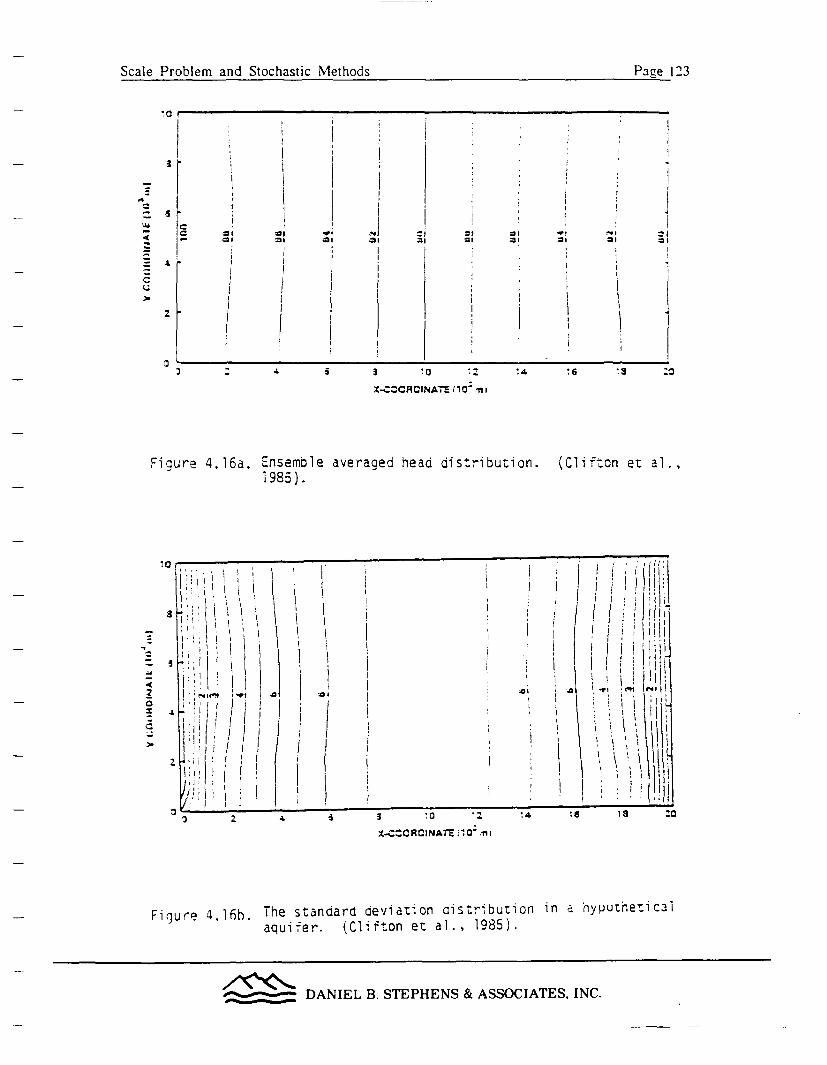
Scale Problem and Stochastic Methods Page 123
3
C
I
I
Ca Z'10
I
I
Ii
I
III
i=1
iii
II
i
I
i
I
0 i
I
I
I
II
A4
* I* I
I I
I
I
iziI
i
z .
aI 4 S 3 0 - 1 1 . a
X-C-CCRCINATE (10; i,,
Figure 4. 16a.
0 , I S1
Ensemble averaged1985).
head distribugion. (Cl i fton et al .,
c..CCORCINATE i1; -n i
Figure 4.16h. The standard deviation aistrribution in -- hyputneticalaquifer. (Clifton et al., 1985).
________ DANIEL B. STEPHENS & ASSOCIATES. INC.
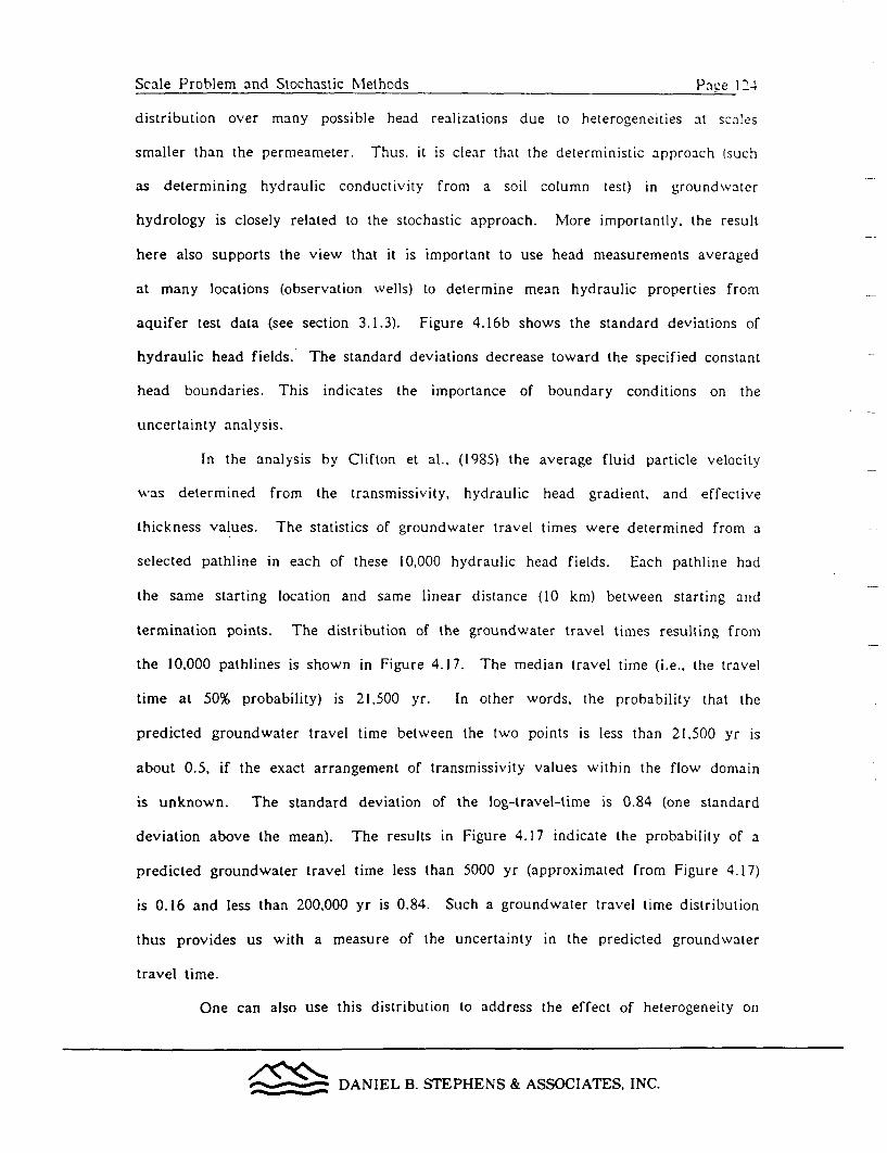
Scale Problem and Stochastic Methods Page 1'4
distribution over many possible head realizations due to heterogeneities at scales
smaller than the permeameter. Thus, it is clear that the deterministic approach (such
as determining hydraulic conductivity from a soil column test) in groundwater
hydrology is closely related to the stochastic approach. More importantly, the result
here also supports the view that it is important to use head measurements averaged
at many locations (observation wells) to determine mean hydraulic properties from
aquifer test data (see section 3.1.3). Figure 4.16b shows the standard deviations of
hydraulic head fields. The standard deviations decrease toward the specified constant
head boundaries. This indicates the importance of boundary conditions on the
uncertainty analysis.
In the analysis by Clifton et al., (1985) the average fluid particle velocity
was determined from the transmissivity, hydraulic head gradient, and effective
thickness values. The statistics of groundwater travel times were determined from a
selected pathline in each of these 10,000 hydraulic head fields. Each pathline had
the same starting location and same linear distance (10 km) between starting and
termination points. The distribution of the groundwater travel times resulting from
the 10,000 pathlines is shown in Figure 4.17. The median travel time (i.e., the travel
time at 50% probability) is 21,500 yr. In other words, the probability that the
predicted groundwater travel time between the two points is less than 21.500 yr is
about 0.5. if the exact arrangement of transmissivity values within the flow domain
is unknown. The standard deviation of the log-travel-time is 0.84 (one standard
deviation above the mean). The results in Figure 4.17 indicate the probability of a
predicted groundwater travel time less than 5000 yr (approximated from Figure 4.17)
is 0.16 and less than 200,000 yr is 0.84. Such a groundwater travel time distribution
thus provides us with a measure of the uncertainty in the predicted groundwater
travel time.
One can also use this distribution to address the effect of heterogeneity on
~ DANIEL B. STEPHENS & ASSOCIATES, INC.

Scale Problem and Stochastic Methods Pace I 2S-
0.1-
a;.
0.ZO.L >-
0.3 X
0.7
0.3
0.3
* I~~~~~~~~~~~~~~~~~.2
10 - 10* a.110IC) IC), 1.0 "a~10 0 1
G;;UNCWATLr.9 TRAVEL 7IME wy
Figure 4.17. Cumulative probability of simulated grounowater traveltimes. (Clifton et al., 1985).
DANIEL B. STEPHENS & ASSOCIATES, INC.

Scale Problem and Stochastic Methods Pa-ze 126
groundwater travel time. if the ergodicity assumption is used. That is. the
probability distribution of ground-water travel time obtained from this analysis is
equivalent to that of the time for a large number of groundwater particles released at
the left boundary to travel across of the flow domain and exit the right boundary
(e.g. Figure 4.15, and 4.16). This groundwater travel time distribution indicates that,
on the average, 50% of the particles will arrive at the ending line within 21.500 yr.
Due to the existence of some fast paths, 84% (one standard deviation less than the
mean) of the groundwater particles will cross the flow domain in less than 200.000
yr. Therefore. the spread of groundwater travel times reflects spatial variations in
fluid particle velocity, i.e., deviations of the velocities from the mean, within the
flow field. In fact, this probability distribution is similar to the concentration
distribution in a soil column tracer test discussed earlier with the exception that this
distribution does not consider velocity variations at scales smaller than the finite
difference block.
When a numerical groundwater flow model is used, the flow domain
generally has to be discretized into many smaller grids. Because there are practical
limits on the total number of grids used to represent a model domain, there will in
turn be some limit on the minimum size of a block. Property values assigned to the
block represent the averages over the block, and consequently variations at subscales
are neglected. The larger the block is the more subscale variability is ignored.
Therefore, the size of block used in the numerical simulation will influence results of
the analysis, regardless of its impact on the accuracy of the numerical solution.
Figure 4.18 illustrates the effect of the size of blocks (zones) on the probability
distribution of groundwater travel time. As indicated in the figure, both the mean
travel time and the standard deviation of log travel time (a measure of the arrival
time variability) decrease as the size of the block increases. In the work by Clifton
et al. (1985), the mean travel increased by 41%, from 16,000 to 23,500 years. when
_______ DANIEL B. STEPHENS & ASSOCIATES, INC.

Scale Problem and Stochastic Methods Pave 127
a
_1 0 4
I._
I <S
I_ 5 :
Q2_
a .8 1
- 0.7
- 0.8
_ as
10j
WICUNOWAT-7.2 -AVP. IW fyr,
Figure 4.13. Effects of finite difference block (zone) size on thecumulative probability or groundwater travel time.(Clifton et al., 1985).
_DANIEL B. STEPHENS & ASSOCIATES, INC.

Scale Problem and Stochastic Methods Page 128
the grid blocks size in the model decreased from 5.0 to 0.5 km. This result is anainl
illustrative of the importance of considering subscale variability in the prediction of
the ground water travel time.
Impacts of the correlation scale of transmissivity values on the groundwvater
travel time distribution were also investigated in the study by Clifton et al. (1985).
The travel time distributions from six random fields with different log-transmissivity
correlation scales are illustrated in Figure 4.19. A constant variance in transmissivity
was assumed in all six cases. As the correlation scale increases, the mean and
standard deviation of log travel time also increase. At first inspection, this result
may not seem intuitively correct, and an explanation is required. Generally speaking,
the heterogeneity is characterized by the magnitudes of both variance and correlation.
That is. a homogeneous medium has a zero variance and infinite correlation scale.
and conversely, a highly heterogeneous medium has a large variance and small
correlation scales. Thus, a variance assigned to a perfectly correlated medium (i.e., a
medium with infinite correlation scale) may strictly represent uncertainty in
measurements of the parameters. For other cases, one can explain the physical
meaning of the results as follows. If the correlation scale is zero, spatial variations
in transmissivity values between the starting and the ending points along the travel
path are statistically independent. This implies that the heterogeneity encountered by
a particle in each realization will be the same regardless of the sequential
arrangement of the transmissivity values. Hence, the arrival times are identical
among realizations. As the correlation scale increases, the sequential arrangement of
the transmissivity values becomes important. This results in different arrival times
among realizations.
Clifton et al. (1985) also found that an increase in the degree of cross-
correlation between transmissivity and effective thickness causes a decrease in the
variability of the predicted groundwater travel times. Independence between
______DANIEL B. STEPHENS & ASSOCIATES, INC.

Scale Problem and Stochastic Methods Pq'a I 'ICScale Problem and Stochastic Methods i~~~~. -n I _7I
I .0
0-,
0.3
0. 7K
.SI
0.5
0. -
IC
0.1
0laQ
GAGUNCWAT- 7RAVF- -IME ~yrt
Figure 4.19. Effects of correlation scalethe cumulative probability of(From Clifton et al., 1985).
of transmissivitv ongroundwater travel time.
_/ ~ _DANIEL B. STEPHENS & ASSOCIATES, INC.

Scale Problem and Stochastic Methods P'ate 130
transmissivity and effective thickness results in a greater \ariability in the predictcd
travel times. The groundwater travel time distribution was found to be sensitive to
the size of the model domain. The average travel time became longer as the width
of the model domain decreased, and vice versa.
In summary, the results of the study by Clifton et al. (1985) shows that
groundwater travel times are sensitive to parameters characterizing the spatial
variability, the scale of representation of model parameters, and the size of model
domain. A major technical drawback of the study is that the calculation of pathline
was not clearly presented. This may have significant impacts on the accuracy of the
predicted travel times, especially if the medium is heterogeneous. Comparisons of the
relative importance of various factors on the groundwater travel time distribution was
absent. This information would be helpful in the analysis of uncertainties in travel
times. Overall, the results of the study are pertinent to the understanding of some
sources of uncertainty in groundwater travel time calculations.
Another interesting analysis of uncertainties in groundwater travel times and
paths due to sample size was carried out by Cole and Foote (1987). In their study, a
hypothetical, two-dimensional, square aquifer with two realizations of hydraulic
conductivity field was used. The first realization represented a real world analog of
the hydraulic conductivity field. It was derived from a block of Nevada topographic
data to ensure that it contained a variety of spatial correlation scales related in a
natural way. The topographic data. which were nearly normally distributed, were
scaled in order to allow them to represent a reasonable range for the logarithm of
hydraulic conductivity. In the second realization, the hydraulic conductivity field
was filtered using a simple moving average technique to remove the high spatial
frequency perturbations in hydraulic conductivity data (i.e. small-scale variations in
K). The filtered data could be viewed as the data collected from large-scale
hydraulic tests in which small-scale phenomena are averaged out. The unfiltered log
DANIEL B. STEPHENS & ASSOCIATES, INC.

Scale Problem and Stochastic Methods Pa-e 131
K data set had a sample mean of 0.0814 and a standard deviation of 1.'8. and the
filtered data have a mean of 0.0821, and a standard deviation of 1.18. In Figure
4.20, a comparison of the unfiltered and filtered log K distribution along a cross-
section is shown. The autocorrelation function for the data set was determined to be
anisotropic. The longest axis of the correlation ellipse was nearly diagonal to the
square aquifer, running from north to south. The anisotropy ratio of the correlation
lengths was about 3. Two flow situations were examined: Case (1) east-west flow,
where east and west sides of the square aquifer were assigned as prescribed head
boundaries, and impermeable boundaries were assigned at the other two sides; Case
(2) south-north flow, where south and north sides of the aquifer were assumed to be
prescribed head boundaries and impermeable boundaries were set for the other two
sides. The flow domain was discretized into 257x257 grids and hydraulic head and
stream functions were calculated using a finite difference model for steady-state
saturated flow. The convective velocity vector was calculated at each grid location
from the stream function (or hydraulic gradient), hydraulic conductivity, and effective
porosity. A particle tracking technique was used to determine groundwater travel
times. Some of the results of the analysis are illustrated in Figure 4.21
Several conclusions were drawn from the results of the analysis by Cole and
Foote (1987). The arrival times of 50% of the total number of particles in both Cases
I and 2 were reduced if the filtered data set was used (Figure 4.21). The filtered
hydraulic conductivity field produced a narrower arrival time distribution because
filtering results in reducing the number of different pathways. According to Foote
and Cole (1987), simulations using the filtered data tended to underestimate the first
arrival of particles if flow was more nearly aligned with the longest correlation scale
of the hydraulic conductivity field (Case 2), and to overestimate the time of arrival if
flow was perpendicular to the direction of the longest correlation scale of the log K
field (Case 1).
_______ DANIEL B. STEPHENS & ASSOCIATES, INC.
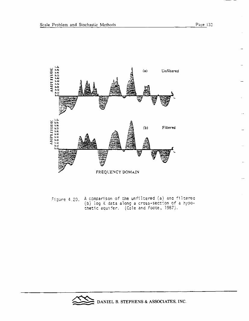
Scale Problem and Stochastic Methods Pa,-,e 137
:A.a
I-u
(a) U-nfltered
= 3.z= -- a-- 3..- 3.3
_; L:
, L &
I2.;.I I
j
4jjIj44j E2
T.- I.Altr-, II
F
(b) Filteredr.,
At,
Ar
v f 11: --5; - I L.
lyw-ww
REQUENCY DOMAIN
-Figure 4,20. A comoarison of the unfiltered (a) ano f:ilterec(b) log K data along a cross-section of a nypo-thetic aquifer. (Cole and Foote, 1987).
________ DANIEL B. STEPHENS & ASSOCIATES. INC.

.'�rnlp Prnhipm and Stncha-,fic Methods Page 1 33a...I Pro.e ... c vtca~i vehd Pag 133.... _ , ................ ,
3
Unfiltered Case
14
4-.
b
S
(a)31
a~I
a .=
t
3C,:
Filtered Case
i
(d)
-LM. Lw.m M&. =I Time Sir UXIC.
LOLM LM M=. .MLX T1Wt STEPS ~X1O1
a
:13
1
I; a� 3
112 (b) (e)
112
n
4t
I
= 3
= A
.mx I m I== .3I 1IfE S7IS MCIiO M. I ' 71? LMT 3x: Go
2/4
(C) R'o
-3!
()
Y4
z IG!
5'1
, -
.U
IL= ;=.= 13LM MMU,- -I.'IME S.Ers (XID
Figure 4.21. Particle arrival versus time curves (for the particles to travel1/4, 1/2, and 3/4 of the distance across the domain) calculatedfor a pulse release of particles from a source in the east-westflow condition. Results are shown for the unfiltered data set(a-c) and for the filtered hydraulic conductivity data set (d-f.(Cole and Foote, 1987).
_______ DANIEL B. STEPHENS & ASSOCIATES, INC.

Scale Problem and Stochastic Methods lIa e 1 34
The results of the simulation are not conclusive because only two realizations
of hydraulic conductivity fields (i.e., unfiltered and filtered) were employed.
However, the effects of the REV assumption (i.e., the properties are uniformly
distributed within the average volume), the scale of hydraulic testing, and size of
spatial discretization in numerical simulations are well manifested in the analysis
inasmuch as the filtering procedure is analogous to the averaging process in deriving
hydraulic parameters from large-scale hydraulic tests. Similar spatial averaging
procedures are often used in numerical models because hydraulic parameters assigned
to each finite element or finite difference block represent the averaged values over
the element or the block. These two conclusions agree with those by Clifton et al.
(1985) (see Figure 4.18). The results of this study again demonstrate the problem
with the groundwater travel times and paths concept.
As pointed out in section 2 dealing with basic concepts in groundwater
hydrology, every property defined in groundwater hydrology involves a volume
(REV). The property of the REV represents an average value over the volume, and
the subscale variation in this property is ignored. The results of the analysis showed
that ignoring the small-scale variability in hydraulic conductivity will result in
underestimating the first arrival of tracer particles, overestimating the mean travel,
and predicting a narrower arrival time distribution (Figure 4.18). Such effects may
play a crucial role in regulating any nuclear waste repository facility, since the
subscale velocity variation affects the fastest path by which groundwater travels. So.
what is the proper volume for defining groundwater travel times and paths in order
that the effects of subscale variations can be safely ignored? If one selects a volume
that is large, then how do we account for subscale phenomena? On the other hand,
if one selects a volume that is too small, then how do we characterize a large-scale
aquifer with the properties defined over such a small volume? This is the dilemma
we face if the concept of groundwater travel times and paths is to be used for
DANIEL B. STEPHENS & ASSOCIATES. INC.

Scale Problem and Stochastic Methods Pace 135
regulatory purposes.
One of the key issues of the high-level nuclear waste repository site
characterization program is determining if large-scale or small-scale hydraulic tests
should be conducted to delineate the fastest path groundwater travel. This issue has
been discussed earlier in various sections of this report, however. additional research
addressing this issue has been presented by Smith and Schwartz (1981b). The
objective of their study is to investigate the uncertainty in predicting mass transport
due to three sources of uncertainties in data input to a model: (I) uncertainties due
to the unknown spatial variation of the medium parameters. (2) uncertainties inherent
in the particular model chosen to account for the heterogeneity, and (3) uncertainties
related to the boundary conditions imposed on the flow domain.
A hypothetical water table aquifer was studied where the sides and bottom
were assumed to be no-flow boundaries for both water and solute, and the water
table represented the upper boundary for the region. A particle tracking model
(Smith and Schwartz, 1980) was used to simulate the transport of a tracer in this
aquifer. Monte Carlo simulation was used to form estimates of the probability
distributions on model output. Hydraulic conductivity and porosity values of the
aquifer were assumed to be statistically homogeneous, and their spatial structure was
represented by a nearest-neighbor model (Smith and Freeze. 1979a). Furthermore,
hydraulic conductivity and porosity were considered to be correlated and lognormally
and normally distributed, respectively. Three hundred realizations of hydraulic
conductivity and porosity fields were analyzed for transport of 600 particles.
Statistics (mean and standard deviation) were computed for the first and last arrival
times, as well as, for the arrival time of the maximum mass.
Most of the results are similar to those by Clifton et al. (1985), and Cole and
Foote (1987). However, Smith and Schwartz (1980) also investigated cases where
large, recognizable, geologic structures (such as stratifications) were present. The
_______ DANIEL B. STEPHENS & ASSOCIATES, INC.

Scale Problem and Stochastic Methods Pa:e 136
aquifer consisted of layers of two distinct materials (sand and silt). WVithin each
layer, hydrologic properties were assumed to be statistically homogeneous processes.
Figure 4.22 shows the schematic diagram of the layered geologic formations with thin.
relatively uniform higher-conductivity layers used in their simulation experiments.
Table 2 summarizes the statistics of simulation results for the two scenarios shown in
Figure 4.22. Results of the simulations showed that the fraction of mass which
moves relatively quickly into the higher conductivity bed determined the initial
arrival statistics. Because a small standard deviation in log hydraulic conductivity
was assigned to the bed, the result is a smaller standard deviation in the initial
arrival time than that in non-layered case. However, uncertainties in predicted
arrival times can still be fairly large because of the sensitivity of transport to the
within-layer heterogeneity. Again, this result is supportive of the position of this
report on the importance of subscale variability. The result also sheds light on the
high-level nuclear waste repository site characterization program. Large-scale
permeable formations have to be identified by geologists or hydrogeologists as
suggested by Williams (1988). However, small-scale tests are also necessary in order
to define the variability within the formations. The subscale variability should then
be treated stochastically.
Schwartz et al. (1983) employed a Monte Carlo technique to analyze
macroscopic dispersion in fractured media. Mass transport in hypothetical two-
dimensional, fractured aquifers was simulated using a particle tracking technique.
Fractures in the aquifers are represented as linear features defined in terms of the
location in space of their midpoints, their orientation with respect to the coordinate
axes, their length, and their aperture. Some of these parameters were considered as
random variables in the analysis. The fracture length distribution was assumed to
have a negative exponential distribution. The distribution of fracture aperture was
considered to be lognormal. Flow in the fractures was idealized as laminar flow
^____ DANIEL B. STEPHENS & ASSOCIATES, INC.

Scale Problem and Stochastic Methods Scale Problem and Stochastic Methods Page 137
MoCturflI
MC - :00 A V: N (-1.20.10.50NP',0 t 3 Y: N1 ~-.00.051.a-zs- !- C SarnoAs A
I N 0.20. 0C-1n 0.'4U0. ).CZI
J_ - .3.40 �' - I 1O
.%- - 0.40 .11 - :0.0
A
;� �a .
'.I
Macrum 2MC -300 A Y: N (-I 20.0.501 N 10.20. 0.=01 ,, -0.40 a - °NP-60O 3 Y: N (-I.45. 20.! ': M (0.20. 0.0O1 >.,,. -0.40 \.,- 12.9
- 125 C Y N (-0.1o. 0.051 vz N (0.25. 0.031 J -0.40 4 \ -:0.0
| ~~~~a
a
MC = number of realizationsNP = number of particles
= = time stepY:NC-1.20, 0.50] = log K; normally distributed with mean -1.20 anc
standard deviation 0.50n = porosityfyn = cross-correlation between log K and n
Ax = average correlation scale in the x direction
Figure 4.22. Schematic diagram of the layered geologic media withthin, relatively uniform higher conductivity layersused in the simulation experiments. (Smith andSchwartz, 1981).
_______ DANIEL B. STEPHENS & ASSOCIATES, INC.

Scale Problem and Stochastic Methods Page 138
Table 2. Comparison oF transport behavior in systems Fith thin, relativelyuniform higher conductivity layers extending across thme basin.(Smith and Schwartz, 1981).
~~.teoium tu
Initial arrival
S. I.~~~~~~~30 ~~6o0Time ot maximum maws
F-- 1 ~~~~1..4O4:4S., 5.60 1.050
U~st :-nval=200
S.. -~~~~ ~~.310 ;90Maximurnm ~as at water
:aoie30.:- 48.4
S~~~~~~~~. ~ ~ ~ iJ31 85Mean .ocauon oC
arrivai:99.0 .~~99.4
Si ~~~~~~~~~~4.4 L~3Standard deviation in
lOcauionT ~~~ ~ ~~~1.0 0.4
Minsturn location-194~~~9 :98.0
______ DANIEL B. STEPHENS & ASSOCIATES, INC.

Scale Problem and Stochastic Miethods Patze 139
through smooth parallel plates so that the cubic law which relates fracture hydraulic
conductivity to fracture aperture could be applied. Sets of fractures were generated
in a rectangular, two-dimensional aquifer with the assumption that the rock matrix
had zero permeability. The aquifer was bounded by two constant head and two no-
flow boundaries. A finite difference model was used to determine the hydraulic
head distribution, and mass transport was then simulated using a particle tracking
technique. The results of the study showed that the mass transport phenomena in
fracture rocks are so complex that the classical macroscopic convection-dispersion
equation does not seem to be appropriate. A single value of dispersivity or
dispersivity function does not appear to characterize correctly the pattern of mass
spreading in a fracture system.
DANIEL B. STEPHENS & ASSOCIATES, INC.

Scale Problem and Stochastic Methods Page 1-0
4.3.2 Conditional Simulation. Conditional simulation is a special kind of
Monte Carlo simulation technique. Unlike the Monte Carlo simulation discussed
above, it imposes sample values at the sample points. That is. in each realization,
parameter values are kept constant and equal to the measured values at a particular
location. Thus, there will be no uncertainty at measurement points.
The complete theory of a conditional simulation procedure based on kriging
is given by Matheron (1973) and Journel and Huijbregts (1978). A schematic
illustration of the conditional simulation is shown in Figure 4.23. Briefly, the
procedures of the conditional simulation are: (1) to generate nonconditional
simulations, that is, to synthesize different realizations of the random field of
hydraulic properties which maintain the actual covariance function that has been
inferred from the data, and (2) to condition of the simulations obtained in the first
step by making the realizations consistent with the measured sample values, The
first step is identical to the Monte Carlo simulation. For the second step, one has to
employ kriging. From the actual sample values, kriging yields an estimate KS (x)
(Figure 4.23a). If x is not a sample point, the true value K(x) is not available, and
the kriging error K(x) - K' (x) remains unknown. However, the true value, K(x),
equals the estimate plus the error in the estimate which we can write as:
K(x) = K' (x) + [K(x) - K' (x)] (4.3.1)
Kriging can be performed using the measured values at the actual sample locations as
data in a given nonconditional simulation (Figure 4.23b). The sample value of the
given nonconditional simulation S(x) can be decomposed as the sum of the kriging
estimate S' (x) and the kriging error, i.e., S(x) - S* + [S(x)-S' (x)]. Since this is
derived from the nonconditional simulation, all terms are known. Note that [S(x) -
S- (x) = 0] at the sample locations. By substituting S(x)-S* (x) for K(x)- K* (x), the
____--_ DANIEL B. STEPHENS & ASSOCIATES, INC.

Scale Problem and Stochastic Methods J�Piage 141
* SAMPLING POINT
Al Z*(x) KRIGING ESTIMATES
"~-~~ 4--- TRUE CONDUCTIVITYFIELD Z(x)
S(x)=S*(x)+[S(x)-S*lNON-CONDITIONAL SIMULATION
a S*(x) KRIGING ESTUIATEOF THE NCS
ONE REALIZATION OF THECONDITIONAL SIMULATION
, Z (x)=Z*(x)+[S(x)-S*(X)]
-- Z*(x) KRIGING ESTIMATES
C.-,
X DISTANCE
Figure 4.23. A schematic illustration of the conditional simulation.
1/1<_1~ DANIEL B. STEPHENS & ASSOCIATES, INC.

Scale Problem and Stochastic Methods iat;,e 1 42
K. (x) for the conditional simulation is defined as:
Ks (x) = K' (x) + [S(x) - S (X)] (4. 3.)
Therefore, K, (x) is consistent with the measured values at the sample points, Ks (x)
and K(x) have the same covariance functions. The average of many conditional
simulations at a given point x is the kriging estimate, and their variance is the
kriging variance.
Generally speaking. hydraulic property fields resulting from conditional
simulation are; (1) smoother than unconditioned fields, but (2) more variable than
kriged fields which essentially represent the conditional expected values.
The first application of conditional simulation to groundwater hydrology
probably was the work by Delhomme (1979). He used 45 transmissivity data
collected in the Bathonian aquifer in Normandy to investigate the effect of
conditioning transmissivity values at sample locations on the uncertainty of the
hydraulic head distribution. The first case he examined was steady- state flow
through a rectangular hypothetical aquifer 10 km in length and 7.5 km in width.
The aquifer was bounded by three impermeable boundaries and one constant head
boundary. A uniform recharge over the aquifer area was assumed. Transmissivity
values were considered to have a lognormal distribution with a spherical
semivariogram as the spatial correlation structure. Thirty sample values were used
with kriging to estimate the transmissivity at unsampled nodes of a 0.25 x 0.25 km
regular grid. Fifty realizations of the logarithm of transmissivity (log T) fields
incorporating the 30 samples were generated. Then, 50 head surfaces corresponding to
the 50 transmissivity conditional simulations were produced by a numerical model.
The results of the simulation indicated that conditioning by 30 log T samples did not
lead to any significant decrease in uncertainty in head values at the center of the
________ DANIEL B. STEPHENS & ASSOCIATES, INC.

Scale Problem and Stochastic Methods l':al e 143
aquifer. This was attributed to the fact that these 30 log T values were samnpled far
away from the outflow boundary which was a major controlling factor of the flow
regime. Conclusions drawn from this study illustrate: (1) the importance of the
locations of the log T samples with respect to the boundary conditions. and (2) that
knowledge of head values at some locations and recharge rates. In addition,
conditioning log T values may be helpful in reducing uncertainties in predicting
hydraulic head values in heterogeneous aquifers.
Case 2 of the study by Delhomme (1979) is the Bathonian aquifer where it is
bounded to the north by the sea. Steep hydraulic gradients occur in the southern
part of the area which are due to local dewatering of mines. Discharge from wells,
rainfall infiltration, interaction with streams, and leakage to or from overlying and
underlying aquifers were considered in the simulation. Two possible sources of
uncertainty on transmissivity were considered: (I) spatial variability and scattered
sampling, and (2) measurement errors in T sample values. A similar approach to
Case I was used. The conclusions drawn from the results of the analysis of Case 2
are: (I) the head surface cannot be reconstructed correctly from only the sample
values of T. and (2) constraints on some head values tend to improve the agreement
between simulated and observed head surfaces, without the transmissivity field
necessarily being correct. Again, the flow rates to and from boundaries play
important roles in reconstructing the head surface. Delhomme finally concluded that
using conditioning on both head and log T values may be necessary in order to
reduce the uncertainty in predicting the true head surface.
Conditional simulations pertinent to NRC's definition of groundwater travel
time and path criterion were conducted by Smith and Schwartz (1981). They used
this technique to study the role of hydraulic conductivity data in reduction of
uncertainty in prediction of mass transport. Two cases were examined. In Case 1,
they investigated the extent to which uncertainties in transport predictions are
________ DANIEL B. STEPHENS & ASSOCIATES, INC.

Scale Problem and Stochastic Methods Page 144
reduced when hydraulic conductivity data act to constrain the possible arrangement
of the heterogeneities. In Case 2, they investigated uncertainties in transport
predictions using a hydraulic conductivity distribution estimated from a limited set of
data.
In the first case. a hydraulic conductivity distribution along a two-
dimensional, vertical cross-section of a hypothetical water table aquifer was generated
using the nearest-neighbor model. They assumed statistical parameters (mean and
variance) to characterize the variability of conductivity. This realization was
assumed to be an analog of the site. Hydraulic conductivity values were sampled in
this realization on a preselected grid, and this data set was used to estimate the
parameters of the hydraulic conductivity distribution. The movement of contaminants
from a hypothetical waste repository was simulated to determine various arrival times
as solute mass exited from the aquifer.
As we described in the previous section (4.3.1), Monte Carlo simulations (300
realizations of hydraulic conductivity fields) were carried out based on the estimated
statistical parameters without considering the conditioning at the sample grid using
sample data. The movement of a swarm of 600 particles in each hydraulic
conductivity realization was simulated using a transport model. The mean and
coefficient of variation (i.e., standard deviation/mean) for each of the times of initial,
maximum mass, and last arrival resulting from the 300 possible realizations were then
analyzed. The results cf this analysis represent the uncertainty in prediction. A
small subset of the hydraulic conductivity values was sampled from the analog of a
real-world site and was then used to constrain the hydraulic conductivity values at
the sample locations. Three sample grids were used: Grid A had 12 sampling points,
Grid B, 24 points, and Grid C, 36 points. Three hundred hydraulic conductivity
fields were simulated in which the hydraulic conductivity values are identical to the
sample values at the sample points.
________ DANIEL B. STEPHENS & ASSOCIATES, INC.

Scale Problem and Stochastic Methods Page I14
Again, the mean and coefficient of variation for each of the arrival time
distributions were analyzed. A comparison of the means and coefficients of variation
of the unconditional and conditional simulations determined the effect of knowledge
of hydraulic conductivity values at sample locations on uncertainty in prediction.
That is, a decrease in the coefficient of variation can be taken as a measure of the
reduction in the uncertainty in prediction. Effects of varying the number of samples
were investigated. Surprisingly, for their data base, results of unconditional and
conditional simulations indicated that knowledge of additional hydraulic conductivity
data did not lead to large reductions in the uncertainty in the velocity field. This
result is relevant to identifying uncertainties in groundwater travel time and in
assessing data needs for site characterization.
The conditional simulations in Case 2 of Smith and Schwartz (1981)
proceeded as follows. From a specified stochastic process with given parameters. a
hydraulic conductivity field was constructed. Hydraulic conductivity values were
sampled from this realization on a preselected grid, and this data set was used to
estimate the parameters of the hydraulic conductivity distribution. A second
realization was generated using these estimated parameters, while the hydraulic
conductivity values were preserved at the measurement points. Mass transport was
then simulated in this second realization. This two-step procedure was repeated over
a set of trials in a Monte Carlo simulation to form the probability distributions of the
arrival times.
Distinct differences exist between Cases I and 2. In Case 1, the parameters
of the hydraulic conductivity distribution were estimated from the hydraulic
conductivity values located on the sample grid. These estimated parameters and the
data set were then fixed for all the realizations in that Monte Carlo experiment. For
the simulation in Case 2, the estimated parameters of the stochastic process varied
with each realization, as different sets of hydraulic conductivity values are located on
_-______ DANIEL B. STEPHENS & ASSOCIATES, INC.
Scale Problem and Stochastic Methods Page 146
the sample grid. The statistical parameters estimated from the available hydraulic
conductivity data are different from those prescribed as the properties of the
ensemble. Thus, errors in estimating the parameters add additional sources of
uncertainty in prediction. That is, a ratio formed between the coefficient of
variation for the arrival times in the Case 2 simulations and a corresponding
unconditional simulation will indicate the extent to which uncertainties are increased
in estimating the mean and standard deviation in hydraulic conductivity. The larger
the value of this ratio, the greater the importance of uncertainties in estimating the
statistical parameters relative to the uncertainty introduced due to the unknown
patterns of spatial variation in hydraulic conductivity. Table 3 summarizes the ratio
for selected transport parameters for the Case 2 simulation. All the ratios are
greater than 1, indicating additional uncertainties due to uncertainty in estimating the
ensemble statistical parameters. However, such uncertainties are reduced as the
number of samples increases.
A general conclusion drawn from the study by Smith and Schwartz (1981) is
that unless a considerable number of field measurements are available to constrain
the patterns of spatial variation in hydraulic conductivity, large uncertainties can be
associated with seepage velocities. Individual hydraulic conductivity measurements do
not reduce the uncertainty significantly because of the dependence of the local
hydraulic gradient on the overall arrangement of heterogeneities within the flow
domain. Smith and Schwartz (1981) suggested that more emphasis should be placed
on in situ measurements of seepage velocity (fluid particle velocity). However,
seepage velocity generally varies with time, and it is difficult to take any
measurement in the field due to slow movement of groundwater. Therefore, their
suggestion may not be practical. Finally, they emphasized that a careful selection of
sample locations should focus on regions where the uncertainty in the seepage
velocity is greatest. A carefully designed. integrated sampling program may play an
DANIEL B. STEPHENS & ASSOCIATES, INC.
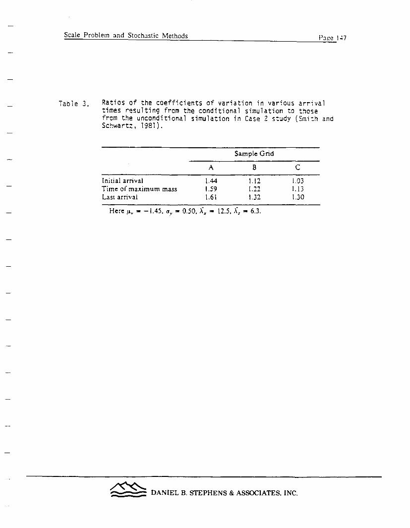
Scale Problem and Stochastic Methods Pq).9 1 27I,.,
Table 3. Ratios of the coefficients of variation in various arrivaltimes resulting from the conditional simulation to thosefrom the unconditional simulation in Case 2 study (Smith andSchwartz, 1981).
Sample Grid
A B C
Initial arrival 1.44 1.12 1.03Time of maximum mass 1.59 1.22 1.13Last arrival 1.61 1.32 1.30
Here u -= -1.45,, ay 0.50, A, - 12.5, A - 6.3.
- ~ -DANIEL B. STEPHENS & ASSOCIATES, INC.
Scale Problem and Stochastic Methods 11.we 1-AS
important role in the reduction of uncertainties in solute transport predictions.
_____ DANIEL B. STEPHENS & ASSOCIATES, INC.

Scale Problem and Stochastic Methods Paste 149
4.3.3 Spectral Analysis. Spectral analysis is generally an analytical approach
which includes perturbation analysis. This approach has been used extensively by
Gelhar and his co-workers (e.g.. Gelhar, 1976: Bakr et al.. 1978; Gutjahr et al..
1978; Mizell et al., 1982: Gelhar et al., 1979; and Gelhar and Axness, 1983; Yeh et
al., 1985a, b, and c; Mantoglou and Gelhar, 1987a, b, and c). To illustrate the
approach, let us consider steady-state flow in a heterogeneous but locally isotropic
aquifer (i.e., the hydraulic conductivity at the scale of core samples is isotropic) with
infinite lateral extent. The governing flow equation is:
a [K a] = 0. i=1,2.3 (4.3.3)
where K is the hydraulic conductivity and is a function of the spatial coordinates.
The Einstein summation convention is used (i.e., repeated indices imply summing over
the range of the indices). If K ¢ 0, equation (4.3.3) can be rewritten as:
a2 h + arnK aha-a~ ax - = 0 (4.3.4)
If the natural log of hydraulic conductivity, InK, and the hydraulic head, h, are
assumed to be second-order stationary stochastic processes, the equation becomes a
stochastic partial differential equation, and InK and h can be represented by means
and perturbations of these values about their means:
h = H + h' E[h] H. and E[h'] - 0 (4 .3.5a)
InK = F + f E[lnK] . F. and E[f] - 0 (4.3.5b)
DANIEL B. STEPHENS & ASSOCIATES, INC.

Scale Problem and Stochastic Methods Place I S0
where H and F are the means of h and InK, respectively. The perturbations are h'
and f for h and InK, respectively. By substituting the representations (equation 4.3.5)
in equation (4.3.4), and taking the expected value of it. we obtain a mean equation:
a2H + aF + aF aH + E f ah= (4.3.6)axiaxi aX1 ax T. L axi ax
Substracting the mean equation from equation (4.3.4) gives:
a2h' af aH + aF ah' E_ af ah' 1 + af ah 0 (4.3.7)axiax i ax, X ax1 axT L axi axi j axi axi
If we assume that the log hydraulic conductivity perturbation f is small (aquifer is
not highly heterogeneous, say, u2 <1.5 (Ababou et al., 1988), it is logical to expect the
head perturbation h will be small. Then, it is reasonable to neglect higher order
terms so that the perturbation equation can be written as:
af AH + a alh' + 0 (4.3.8)ax; axi ax3 ax3 axiaxi
This approximate equation describes the relationship between the perturbations in InK
and h' in a steady-state flow with mean gradients, aH/axi.
The above mathematical procedures are equivalent to visualizing the
heterogeneous aquifer as a collection of finite elements, and flow in each element is
described by the governing flow equation with a constant hydraulic conductivity
value. A collection of an infinite number of elements whose hydraulic conductivities
are spatially correlated is then equivalent to an ensemble in the stochastic sense.
____ DANIEL B. STEPHENS & ASSOCIATES, INC.

Scale Problem and Stochastic Methods Pice 151
Taking the expected value (ensemble average) of equation (4.3..') wK ith stochastic
parameters is tantamount to ignoring the details of the flow behavior in each element
but examining the average behavior of the flow in all the interconnected elements.
The perturbation equation thus depicts the deviation of the flow from the mean flow
only.
Now, the problem is how to solve the perturbation equation (4.3.8) and here
the spectral method comes into the play. The spectral representation theorem
(Lumley and Panofsky, 1964) states that if a stochastic process y(x) is second-order
stationary, there is an essentially unique complex-valued, random distribution Z(k) on
the frequency axis such that:
Y(x) = I eikXdZ(k) (4.3.9)
where i is a complex number and dZ is a generalized derivative of Z(k). Equation
(4.3.9) is an example of a Fourier-Stieltjes integral. Furthermore, this process Z(k)
represents complex-value random variables in a wave number k domain. In addition,
this Z(k) process is related to covariance behavior as discussed below. More
specifically, equation (4.3.9) simply is the inverse Fourier transform of Z(k). or Z(k) is
the Fourier transform of the variable y(x) in the spatial domain. By doing this
transformation, we have tranformed the variable from the spatial domain to the wave
number domain. A physical analogy can be drawn with the effect of a glass prism
on sunlight, as shown in Figure 4.24. A beam of white light can be regarded as a
complex wave form changing with time, and composed of many colors (or
wavelengths) of light. A prism acts as a frequency analyzer and separates the beam
into its components, which appear as a rainbow display. Each colored band is
separated from its neighbor by an amount proportional to the difference in their
DANIEL B. STEPHENS & ASSOCIATES, INC.

Scale Problem and Stochastic Methods Page 152
I z n \( f
Figure 4.24.. A prism acts as a frecuency analyzer, transforming -nite
light (time domain) into its constituent spectrum of
colors (frequency domain). Note the signals in zrie fre-
quency aomain are uncorrelatea. (Davis, 1973).
DANIEL B. STEPHENS & ASSOCIATES, INC.

Scale Problem and Stochastic Methods Paze 1 53
wavelengths or frequencies, and the intensity of each band is proportional to the
contribution of that particular wavelength to the total intensity of the original beam.
Examining the spectrum of a light source may tell us many things: the composition of
the source, its temperature, nature of the material through w hich the light passed,
and so forth.
By the same token, examining the spectrum of spatial data may tell us a
great deal about its nature and origin, information which may not be apparent in any
other way. However, in this spectral analysis, the purpose of taking the Fourier
tranform of the spatially correlated process y(x) is that after the transformation, Z(k)
has been separated from its neighbor so that it is uncorrelated and the mathematics
become easlier. Since Z(k) is uncorrelated, it has the following properties:
E[dZ(ki)dZ- (k2)] = 0. if k1 o k,
E[dZ(kl)dZ- (k2)] = S(k) ki = k2 (4.3.10)
where dZ* is the complex conjugate, and S(k) is the spectrum of y which is merely
the Fourier transform of its autocovariance function:
S(k) = 2 { elike c(X) d6 (4.3.11)
Therefore, the inverse Fourier transform of the spectrum S(k) thus gives:
00
cov[ y(x+V)'5(x) I = c(M) = eikJ S(k)dk (4.3.12)
________ DANIEL B. STEPHENS & ASSOCIATES, INC.

Scale Problem and Stochastic Methods Page 154
Using the representation theorem for the perturbation terms f and h', and assuming
uniform flow, equation (4.3.8) can be rewritten in terms of dZ processes:
iL d k (4.3. 13)dZh= k
where J is the mean gradient in the x direction, aR/ax and is assumed to be
constant. Using the properties of the dZ processes, one can derive the relationship
between the input and output spectrums, Sh'h' and Sff, respectively. That is:
2 -= (4.3.14)
By applying the inverse Fourier transform to the above equation. one thus obtains the
head covariance functions, ch'h0(0). in terms of the hydraulic conductivity covariance
function, cff((). If one uses a simple stationary three-dimensional covariance function
for InK, i.e.:
cff(V) = o2 exp -[2*/x2 + 22/x2 + 32px ]i/2 ] (4.3.15)
where X), X2, and X3 are the correlation scales in xl, x2 . and X3 respectively, the
corresponding spectrum is
ar 2 IX 21k3Srr(k) - f(..6
fr2k4(1 + k2 X2)2 (4.3.16)
________ DANIEL B. STEPHENS & ASSOCIATES, INC.

Scale Problem and Stochastic Methods Pavze 155
If we assume the hydraulic conductivity covariance function is isotropic (i.e., \1 =\-
- X3 ) and take the Fourier transform of (4.3.14). the head Variance, a! . is related to
the variance of the hydraulic conductivity. ar2 by:
= ch'h' (0) J J2 Ur 2 X2 (4.3.17)
The variance equation, (4.3.17), provides us with information on how the
spatial variation in hydraulic conductivity affects the spatial variation in hydraulic
head. In other words, it provides us with a measure of the deviation of hydraulic
head from its mean value predicted using an effective hydraulic conductivity.
The spectral approach is also useful for deriving the effective hydraulic
conductivity for such a stochastic random porous medium. To derive the effective
hydraulic conductivity, we will again conceptualize the heterogenoeus aquifer as a
collection of many finite elements with spatially correlated hydraulic conductivity
values in which the flux is assumed to obey Darcy's law. Thus, the average flux
over the entire heterogeneous aquifer then becomes the expected value of all the
fluxes from each individual element within the aquifer. That is:
E[ qj ] i -E E Kgh E K ef aH + ah.1 (4.3.18a)
Using a series expansion for er. (4.3.18a) becomes:
'-Kg ED I . S P N AS2 S IAT I
-- DANIEL B. STEPHENS & ASSOCIATES, INC.
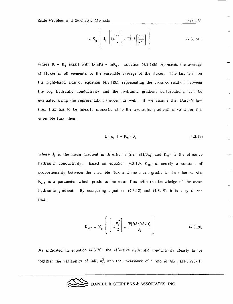
Scale Problem and Stochastic Methods stag1e I 3 0Scale Problem and Stochastic Methods Pnt�e 1�6
Kg J 1+, E~f[4x- (4.3. 1 Sh
where K - Kg exp(f) with E(lnK) = InK2. Equation (4.3.18b) represents the average
of fluxes in all elements, or the ensemble average of the fluxes. The last term on
the right-hand side of equation (4.3.18b). representing the cross-correlation between
the log hydraulic conductivity and the hydraulic gradient perturbations, can be
evaluated using the representation theorem as well. If we assume that Darcy's law
(i.e., flux has to be linearly proportional to the hydraulic gradient) is valid for this
ensemble flux, then:
E[ qj Kff Ji (4.3.19)
where Ji is the mean gradient in direction i (i.e.. 8H/axi) and Keff is the effective
hydraulic conductivity. Based on equation (4.3.19), Keff is merely a constant of
proportionality between the ensemble flux and the mean gradient. In other words,
Kerr is a parameter which produces the mean flux with the knowledge of the mean
hydraulic gradient. By comparing equations (4.3.18) and (4.3.19), it is easy to see
that:
Keft = K [ + Gf ] -E[f(ah/axi)] (4.3.20)
As indicated in equation (4.3.20), the effective hydraulic conductivity clearly lumps
together the variability of InK, or2 and the covariance of f and ah'/axi, E[f(ah'/axj)i,
________ DANIEL B. STEPHENS & ASSOCIATES, INC.

Scale Problem and Stochastic Methods Pace 157
which varies with flow. Therefore. the effective hydraulic conductivity is not a
simple arithmetic average of all hydraulic conductivity values of individual elements,
but it depends on the flow regime as well.
Using the spectral technique discussed above, Bakr et al. (1978) analyzed the
effects of spatial variability on steady-state groundwater flow. Closed forms of head
variance expressions were derived for one- and three-dimensional flow fields in
which hydraulic conductivity is a spatially-varying stochastic process. Several
important conclusions were drawn from the results of the study. Hydraulic head
distribution tends to be smooth due to the damping effect of the groundwater flow
system. That is, the head values are correlated over a much longer distance than the
hydraulic conductivity values. The head values are anisotropic (i.e., correlated over
a longer distance in the direction perpendicular to the flow direction.), even if the
hydraulic conductivity field is statistically isotropic. The head variance can be
related to the variance of InK by:
al,= g'2 Jr X2 (4.3.21)
where /3 is a constant: I for one-dimensional flow, 1/3 for three-dimensional flow, J
is the mean hydraulic gradient, ar2 is the variance of the natural logarithms of
hydraulic conductivity, and X is the correlation scale. The equation indicates that the
variability in head predicted by a three-dimensional model is smaller than that
predicted by a one-dimensional model. This means that a three-dimensional model
would be much more appropriate for analyzing uncertainties in groundwater travel
times and paths. Furthermore, it is manifest from equation (4.3.21) that studying the
correlation scale is important in the calculation of head variance or uncertainty in
head prediction as discussed in the section dealing with Monte Carlo simulation.
________ DANIEL B. STEPHENS & ASSOCIATES, INC.
Scale Problem and Stochastic Methods Pave I 8
Gutjahr et al. (1978) extended Bakr's study to define effective hydraulic
conductivity for heterogeneous InK fields. They concluded that the effective
hydraulic conductivity in one-dimensional flow, perpendicular to layerings, is the
harmonic mean:
_a12
Ke = K e f (4.3.22)
where Kg is the geometric mean of K. and a72 is the variance of InK. and the
arithmetic mean for flow parallel to beddings, i.e.:
C2/2Ke = Kg e f (4.3.23)
In the three-dimensional flow situation, the effective hydraulic conductivity is given
by:
a21a 2/6Ke -Kg e f (4.3.24)
which is slightly greater than the geometric mean. They suggested that the geometric
mean of K may be a good estimator for the effective hydraulic conductivity values
for field situations.
Both analyses by Bakr et al. (1978) and Gutjahr et al. (1978) assumed
statistical isotropy for the random hydraulic conductivity field. Gelhar and Axness
(1983) extended the analyses by Bakr et al. (1978) and Gutjahr et al. (1978) to
investigate the effective hydraulic conductivity of large-scale aquifers in which the
hydraulic conductivity field is assumed to be statistically anisotropic. They showed
________ DANIEL B. STEPHENS & ASSOCIATES, INC.

Scale Problem and Stochastic Methods lPave 159
that the effective hydraulic conductivity, in general, is a second-rank symmietric
tensor whose principal components depend on the ratios. XI/\, and \,/\3. Figure
4.25 shows that the anisotropy ratio for the case with XI = X# $ X3 is dependent on
the degree of variability of hydraulic conductivity in terms of the variance of InK as
well as the geometry of the heterogeneity as characterized by the ratio of WI/X 3.
The effective hydraulic conductivities and head variance derived from the
spectral analysis may have important practical implications on the prediction of
groundwater travel times and paths. Generally speaking, there is a limited number
of hydraulic conductivity values available for determining accurately the groundwater
travel times and paths. As a first step toward solving such a complex problem. one
may use the limited amount of data to determine the variance of InK, and thus the
effective hydraulic conductivity, using one of the equations (4.3.22). (4.3.23), or
(4.3.24), depending on the dimensionality of the model. The mean flow behavior thus
can be determined. Correlation scales can be estimated from the available data by
using autocorrelation analysis. With an estimated mean gradient, variance of InK.
and correlation scales, the head variance in a statistically isotropic medium can then
be determined, using equation (4.3.21). If there is no hydraulic conductivity data
available, one might be able to resort to the known variances and correlation scales
of similar kinds of materials reported in the literature (see table 2 ). The calculated
head variance can be used as a measure of the error in the model as the result of
unmodeled aquifer heterogeneity (i.e., the result of using effective hydraulic
conductivity). Therefore. the head variance is an appropriate model calibration target
to study for defining the detailed hydraulic conductivity distribution, provided that
other sources of error are also considered. The hydraulic conductivity field obtained
from the calibration may then be used to determine groundwater travel times and
paths. A similar application of the above spectral results to field problems was also
illustrated in the paper by Gelhar (1986).
________ DANIEL B. STEPHENS & ASSOCIATES, INC.

Scale Problem and Stochastic Methods Scale Problem and Stochastic Methods Page 160
o00
50
20
1<1310
2
1
2
Figure 4.25. Anisotropy ofa function of
ratio, he /rc3the principal
effective hydraulic conductivity asthe variance of InK, off, and aspectfor the case ' 1=x2. K , and K: areeffective hydraulic coiductivie in
xl and x3 directions, resoectively.
DANIEL B. STEPHENS & ASSOCIATES, INC.

Scale Problem and Stochastic Methods Page 161
As emphasized many places in this report, the arrival time of a ccrtalin
concentration of a tracer is similar to the groundwvater travel time. The difference is
that no tracer particles are involved, and the concentration is defined as the ratio of
the weight of newly-arrived groundwater particles to the total weight of groundwvater
in the sample volume. If one has this concept in mind, it is clear that the
nonreactive solute transport equation is the most appropriate model for determining
the groundwater travel time. The use of the effective hydraulic conductivity predicts
only the arrival of the center of the mass plume, and the arrival of fast moving
groundwater particles due to subscale velocity variation is ignored. To analyze the
effect of velocity variations on solute transport, the macrod ispersion concept has to be
introduced. This macrodispersion approach is analogous to the analysis of molecular
diffusion at the microscopic scale discussed in section 2.6.
In order to use the macrodispersion approach, macrodispersivity must be
defined. The dispersivity value at the laboratory scale can be related to the
variation in grain size. Similarly, macrodispersivity can be related to the variation in
hydraulic conductivity values at scales much smaller than the REV of the stochastic
random field. The relationship between the macrodispersion and local-scale hydraulic
conductivity variations was derived by Gelhar and Axness ( 1983) using a spectral
analysis which will be discussed in the following section.
To examine the theory of macrodispersion, we will assume that the general
equation describing transport of an ideal conservative solute by a fluid with constant
density and viscosity in a saturated, homogeneous, three-dimensional porous media of
constant porosity, n, is:
At~~ Fj x axj~cq ] i~-1.3 (4.3.25S)
_______DANIEL B. STEPHENS & ASSOCIATES, INC.
Scale Problem and Stochastic Methods Page 162
where the standard Cartesian summation convention of Einstein is used and c is the
concentration of the transported solute, qj is specific discharge in the xl direction: EJ
is a local bulk dispersion coefficient tensor equal to nD,1 ; and Dj is the local
dispersion coefficient tensor. If Dij is isotropic (i.e.. the dispersion coefficient values
are the same in all directions), then it is equivalent to Dd defined in Section (2.6).
The local scale used here refers to the size of the volume (REV) over which the
measured hydraulic conductivity is obtained. For example, if hydraulic conductivity
is measured from a core sample, the local scale represents the size of the core.
Thus, the local dispersion coefficient stands for the velocity variation at scales less
than the size of the core sample (it includes molecular diffusion). Similarly, a local
dispersion coefficient can be used to represent the velocity variation at scales much
smaller than the scale at which the transmissivity is defined.
Conservation of total mass requires:
qi = 0 (4.3.26)axi
If a steady state condition is assumed (i.e.. nac/at = 0), equation (4.3.25) becomes:
acq j _____
8 i= Eij ax2ax (4.3.27)
This equation is assumed to be adequate to describe the local-scale dispersion. In a
large-scale heterogeneous aquifer, the log hydraulic conductivity. f; specific
discharge, q; and concentration, c, are assumed to be stochastic processes. These
parameters can be decomposed into a mean part and a perturbation part, i.e.:
___ DANIEL B. STEPHENS & ASSOCIATES, INC.
Scale Problem and Stochastic Methods Page 163
c = c + c,
f = f + fP
q= Qi + q'= i=.2.3 (4.3.S)
where the head and the prime represent the mean and the perturbation, respectively.
Substituting the above expressions into (4.3.27), one obtains:
a [(c + c')(Qi + q'i)] - Ej a2 + C] (4.3.29)[(i c 1 =E axiax.
Because the parameters are stochastic processes, equation (4.3.29) describes
concentration profiles in many realizations of possible heterogeneous aquifers (i.e.,
ensemble). Expanding terms and taking the expected value of the equation (i.e.,
taking the ensemble average) produces the mean equation:
a " c aE[q'c'] - E. ae (4.3.30)
In other words, this is a transport equation which describes the mean profile of all
the possible concentration profiles resulting from each realization of a heterogeneous
hydraulic conductivity field. Comparing this equation to equation (4.3.25), which is
the classic convection-dispersion equation, it should be evident that the first term in
the left-hand side of the equation is the convective flux associated with the mean
flow or specific discharge, and the second term is an additional flux, E[q'ic']. This
mass flux is defined as the macrodispersive flux resulting from the perturbation of
velocity which is caused by the heterogeneity of the aquifer, neglected at the size
where the effective hydraulic conductivity was defined.
______ DANIEL B. STEPHENS & ASSOCIATES, INC.

Scale Problem and Stochastic Methods Page 164
If this macrodispersive flux is Fickian in nature, that is. this flux is linearly
proportional to the mean concentration gradient (equation 2.6.1). and if the mean flowv
is aligned in the xi direction so that q = q $ 0 and q2 '3 = 0, we may then
write:
E[q'c'] = -q Aij 3 8 (4.3.31)
where A1j is the macrodispersivity tensor and q is the magnitude of the specific
discharge vector. The work by Gelhar and Axness (1983) derived expressions for
the Aij term, relating A1j to the variation in hydraulic conductivity, f'. This task
was carried out by using the perturbation technique and the spectral representation
theorem as used in the derivation of the effective hydraulic conductivity analysis.
One of the results shows that:
UaXAll =f2 (4.3.32)
where All is the longitudinal macrodispersivity. uof is the variance of f, X is the
correlation scale of statistically isotropic porous media, and y is the flow correlation
factor which depends on the direction of the mean flow and the orientation of the
heterogeneity.
The practical implication of Gelhar and Axness's work is that the
macrodispersivity values may be estimated from the knowledge of the variation of
local-scale hydraulic conductivity values without conducting a large-scale field tracer
experiment to determine the dispersivity values or the groundwater travel time.
Generally speaking, a large-scale field tracer experiment is impractical in terms of
____,___ DANIEL B. STEPHENS & ASSOCIATES, INC.

Scale Problem and Stochastic Methods Page 165
the time span required for such an experiment. However, local-scale hydraulic
conductivity values are frequently measured in many aquifers. Data are available
but limited. Hence. the macrodispersivity approach may provide a practical solution
to many pollution problems (such as the high-level nuclear waste site characterization
program).
However. the macrodispersivity approach produces the mean concentration
profile only, as indicated by c in equation (4.3.30). The mean concentration profile
represents the average values of concentration profiles occurring in many different
aquifers (i.e., ensemble average, see section 2.6.1). As a result, the actual
concentration profile observed in an aquifer may be quite different from the
predicted one using the macrodispersivity. For example, Figure 4.26 shows the
differences between an observed concentration distribution in the Borden sandy
aquifer and an ensemble averaged (or mean) concentration distribution calculated from
the classic convection-dispersion equation with macrodispersivity values. Determining
the difference between the two profiles is necessary. To evaluate the difference,
Vomvoris and Gelhar (1986) analyzed the mean concentration variance. They found
that the concentration variance is proportional to the mean concentration gradient and
to the variance and correlation scales of log-hydraulic conductivity; it is inversely
proportional to local dispersivity values. The results imply that the concentration
variance could be large depending on the magnitude of the parameters.
Before we illustrate the practical application of the macrodispersion theory to
the groundwater travel time problem, recall that the concentration is simply the
weight ratio of the newly arrived groundwater to the groundwater (including "new"
and "old" water) in a sample volume. If the statistical parameters of the hydraulic
conductivity distribution are known, either estimated from a limited amount of data
or obtained from information from other similar aquifers, one can then calculate the
breakthrough curve at the accessible environment using equation (4.3.30) and
DANIEL B. STEPHENS & ASSOCIATES, INC.

IZ-1a DnNlam nnA 1;Ztnr-hn-ztic Methndq Page 166- 1. . I _- -- __
50 _
40
30 -
20
0
Figure 4.26.
Y(m)
A schematic illustration of an observed depth-averagedconcentration profile (solid) and a mean profile (dash),calculated from the macrodispersion equation (modifiedfrom Sudicky, 1986).
~~ DANIEL B. STEPHENS & ASSOCIATES, INC.

Scale Problem and Stochastic Methods Page 167
macrodispersivity values. This concentration breakthrough curve represents the
arrival time distribution of different amounts of "new" water. Consequently, if a
proper concentration of a tracer is defined as a criterion, then the arrival time can
be defined. For the reason that the calculated concentration is the mean
concentration. one should use the equations provided by Vomvoris and Gelhar (1986)
to determine the variance of the mean concentration. An error band (plus or minus
one concentration standard deviation about the mean concentration) can be calculated
which indicates the range of the uncertainty in the mean concentration profile.
Hence, the uncertainty in groundwater travel time is quantified.
Similar research on macrodispersion has been presented by many other
researchers (e.g., Dagan, 1985, 1986, 1987; Neuman et al.. 1986; Winter et al., 1984;
Matheron and De Marsily, 1983). Dagan (1987) used the Eulerian velocity field to
derive formulas for the time-dependent macrodispersivities in two-dimensional planes
and three-dimensional aquifers. This approach is similar to Taylor's theorem on
diffusion dicussed in section 2.6. However, in Dagan's analysis, the velocity field is
related to the heterogeneity structure of the hydraulic conductivity field through the
governing groundwater flow equation. The hydraulic conductivity field is considered
to be statistically isotropic. For early time periods (i.e., t << X/v). the spatial
concentration variances (the square of the standard deviation of the plume
concentration distribution: this is similar to the w2 in section 2.6.1) are given by
a2 (t) _ 8 a2 v2 t2 + 2 DL t
and a22 (t) = a233 (t) = I a2 v2 t2 + 2 DT t (4.3.33)22 33 15 YTt
for three-dimensional flow, where a2 a222, and a2 are the concentration variances inD' 22B 33
DANIEL B. STEPHENS & ASSOCIATES, INC.

Scale Problem and Stochastic Methods Paz e 16S
the direction of flow, and lateral directions. respectively. Local-scale dispersion
coefficients in the longitudinal and the transverse directions are DL and DT.
respectively. v is the mean velocity, t is time, and N is the correlation scale of the
hydraulic conductivity field. U2 represents the variance of the natural log ofV
hydraulic conductivity in three-dimensional flow and the variance of the natural log
of transmissivity in two-dimensional flow. The results of the two-dimensional flow
anaylsis are:
0.2 3 o2v2 t2=av~t
°22 = I G2 V2 t222 8Y (4.3.34)
For large time periods (i.e., t>>X/v), the three-dimensional results are:
all 20.2 vXt + 2DL t
0.~j u2., 2 a2X2 t22 33 3 Y (4.3.35)
and the two-dimensional results.
a02 o 20.2 Xvt 1 - 31n(vt/X)]I L 2vt/X I
a02 a2 2 N2 [ ln(vt/X) + 0.933 ]22 - y (4.3.36)
Note that the concentration variances (equations (4.3.33) and (4.3.34)) for early time
____-=_ DANIEL B. STEPHENS & ASSOCIATES, INC.

Scale Problem and Stochastic Methods Page 169
periods depend on t2, implying the macrodispersion coefficient grows with time. For
late time periods, the concentration variances (equations (4.3.35. and 4.3.36)) are a
function of t only. This relationship implies that the macrodispersion coefficient is
constant over time. Moreover. equations (4.3.33 - 4.3.36) do not predict the shape of
the concentration plume but its relative size. Thus, no classic convection-dispersion
which assumes the validity of Fick's law is used.
In generally, these results compare favorably with those obtained from a
field tracer experiment (Sudicky, 1986) conducted in a sand aquifer in Canada (see
Figure 4.27). A recent field tracer experiment by Garabedian (1987) in a glacial
outwash aquifer also indicated that the stochastic results (i.e., Gelhar and Axness,
1983; and Dagan, 1987) are suprisingly robust, regardless of many assumptions used
in the development. However, the robustness may be attributed to the fact that the
variance of log hydraulic conductivity in those two aquifers is small so that the first-
order approximation used in stochastic analysis is justifiable. The validity of the
stochastic results, the reviewers of this report believe, still remains to be tested with
tracer experiments in many different geologic environments.
Overall, the major advantage of the analytical approaches by Gelhar and
Axness (1983), and Dagan (1987) is that they provide us with an explicit formula
showing the relationship between the variance of inputs (such as hydraulic
conductivity) and the head variance, or mean concentration profile and its variance,
without conducting numerous computer experiments as required by the Monte Carlo
simulations (such as Clifton et al., 1985; Smith and Schwartz, 1980, 1981a and b).
Additionally, the results of the analytical approach (i.e.. Gelhar and Axness. 1983)
also give us an explicit way to estimate the effective hydraulic conductivity and the
macrodispersivity values of large-scale aquifers if the statistical parameters
characterizing the variability of the small-scale hydraulic conductivity values are
known. The major drawback of the method is that the solution (or the formula)
/_______ DANIEL B. STEPHENS & ASSOCIATES, INC.

Scale Problem and Stochastic Methods Scale Problem and Stochastic Methods Page 170
S0L=7E TANsi"'Jmr sT G~OLNWATT
-
S0-
Z66-
.
II
t
-1
I
IIi
IIi
I
II
a
0
-
I I
C '>c 400 600
iME C(ays)
LONGITUDINAL DIRECTION
aco 'ccc
Or
L
0~~~~~
0 20 4Co 6CC aco D oCO
NIME ' Oays ITRANSVERSE DIRECTION
Figure 4.27. A comoarison of observed (dots) and theoretical (line) sDatialconcentration variance in the longitudinal and transverse airec-tions (Dagan, 1987).
w DANIEL B. STEPHENS & ASSOCIATES, INC.

Scale Problem and Stochastic Methods Pace 171
may be valid only for small values of variations in hydraulic conductivity because of
the omission of product terms in the analysis. Several studies have shown the results
to be valid even for the variance of f = 1. Therefore, one may expect the results
from the spectral analysis to be valid for most unconsolidated materials wvhere the
variance in f may be less than 1. For cases where a large variance in f is expected
(such as in fractured rocks where the variance of InK has been reported to be about
8.7, (Neuman, 1987), the validity of the method remains to be tested. The other
drawback of the spectral approach is the stationarity assumption used in the analysis.
In a basin-scale aquifer, the hydraulic conductivity field is likely to be nonstationary
because of changes in deposition environments which may contain heterogeneities of a
variety of scales, if the scale of our measurement is much smaller than the basin
scale. Moreover, the validity of the classic convection-dispersion equation for large-
scale problems is still under debate (see for example, Yeh, 1987). So. is it valid to
apply such the results of the spectral analysis to these field problems?
It is generally agreed that the validity of the stochastic results still remains
to be tested with tracer experiments in many different geologic environments. \We
previously noted a field experiment to validate the stochastic approach in an alluvial
aquifer is currently in progress in Mississippi (Betson et al., 1985). We are unaware
of similar experiments in unsaturated fractured rock. However, in the vadose zone
there are two field-scale experiments in progress in New Mexico which are designed
to evaluate multi-dimensional transport models in unsaturated media (Stephens et al.,
1984; Wierenga et al., 1986).
DANIEL B. STEPHENS & ASSOCIATES, INC.
Scale Problem and Stochastic Methods Pagze 172
4.3.4 Fractal Approach. In the past few years. geohydrologists and soil
scientists have employed statistics to characterize the spatial variability of hydrological
properties of geologic formations. Most of the hydrologic properties were found to
be correlated over a large distance. Furthermore, many experimentally-determined
variograms or autocorrelation functions of soils and geological data, exhibit some
nugget effects. These nugget effects are generally viewed as a result of small-scale
random noises which are spatially uncorrelated. This view implies that all variation
within the closest sample spacing is infinitely erratic and possesses no spatial
structure whatsoever. Although part of the nugget effect can be attributed to
measurement errors which are likely to be spatially independent, experience shows
that most of the noise at the macroscopic scale could be spatially correlated at the
microscopic scale. This implies that the variability of hydrologic data exists in all
scales and has a correlation structure at each scale (Dagan, 1986; and Gelhar, 1986).
This scale phenomena was illustrated in Figure 4.13. In other words, the hydrologic
data have a nested correlated structure. To analyze such a data set. a fractal
approach has been proposed.
Fractals are based on the idea of 'self-similarity'; that is, the variations at
one scale are manifested at another scale in similar ways. In other words. the
irregularity of a process is independent of the scale of measurement. For example,
the variation in effective hydraulic conductivity obtained from large-scale hydraulic
tests should be similar to that from small-scale tests, at least according to the fractal
concept. This self-similarity implies a long-range correlation structure in geostatistics
terminology. That is, no matter how the size of the hydraulic test varies, the
correlation between adjacent samples remains. For example. in Euclidean or classical
geometry, the length, L, of a straight line can be easily determined by:
L = N e (4.3.37)
DANIEL B. STEPHENS & ASSOCIATES, INC.
Scale Problem and Stochastic Methods Paoe 173
where N is the number of measuring units of length e. If we halve the size of c. N
will increase by a factor of two. Therefore. the length. L. is constant and
independent of the scale of the measurement.
However, the Euclidean concept of a constant distance between two points
independent from the scale of measurement may not be valid. Consider measuring
the distance of a straight line between San Francisco and Washington. D.C. The
distance as viewed by a person in outer space is essentially the length of a straight
line between the two cities. The effects of topographic variation are completely
neglected. However, the distance measured by a person on the ground will be much
longer because this person has to consider the topographic variation of the land
surface. Now, if we imagine the person is shrunk to the size of an ant. the distance
between the two cities will then be even greater than that a normal-size person
would experience, because an ant-size person has to consider not only the large-scale
topographic variations such as hills, depressions, and mountains but also small-scale
topographic variations such as heights of pebbles, rocks, and depths of cracks. The
distance between the two cities, therefore, seems to grow infinitely as the scale of the
measurement continuously decreases. This implies that the distance depends on the
scale of the observation. This conclusion is based on the assumption that the small-
scale topographic variation persists as the scale of the observation is reduced.
If the distance between two points varies with the scale of measurement, one
may then ask the question: can we relate the distance between two points measured
at our scale to those at scales different from ours? If the answer to the question is
positive, we will then be able to predict phenomena at any scale, based on what we
observed at our scale.
If we now assume that the topographic variations at all scales are self-
similar, the distance between the two cities encountered by an ant-size person can
then be scaled so that it is equivalent to that encountered by a normal-size person.
DANIEL B. STEPHENS & ASSOCIATES, INC.

Scale Problem and Stochastic Methods Page 174
This concept is illustrated in Figure 4.28. Suppose the distance between two points
A and B measured at a scale, e, is defined as L(e). A straight line distance. °.
represents the distance measured at a scale E=i (Figure 4.28a). The number of
measurements, N, is 1. If the measurement scale is reduced to 1/3, the topographic
variation at this scale will show up as indicated in Figure 4.28b. The distance
between points A and B becomes 42/3 (i.e. N = 4). A further reduction of the
measurement scale to 1/9 of I reveals even more detailed topographic variation
(Figure 4.28c). The number of measurements, N. required to measure the distance,
then, is 16. If the measurement scale is further decreased to 2/27, the topographic
variation at this scale is shown in Figure 4.28d. In this case, N is 64. Note that the
topographic variations in all the scales are similar in shape. Now, we plot the
measurement scale, e, versus N on log-log paper. A linear relationship between logE
and log N is found (Figure 4.29). That is:
log N - -D log e or N = f-D (4.3.38)
where D is the slope of the line on the log-log plot. For the example, D is equal to
1.2618. This slope, D, is called the fractal dimension (Mandelbrot, 1983). In general,
I < D < 2. If D - 1, N is inversely proportional to the measurement scale e, this
indicates that the line is a topologically one-dimensional object. In other words, the
topographic variation is independent of the scale of measurement. In the limiting
case of D - 2, the line will be so irregular that it fills a plane (Mandelbrot, 1983).
Again, here we are assuming that the topographic variation is self-similar at all
scales. This is the most important property of the fractal geometry. Now. if we let:
F - NeD (4.3.39)
DANIEL B. STEPHENS & ASSOCIATES, INC.

Scale Problem and Stochastic Methods Page 1 75Scale Problem and Stochastic Methods Page 175~~~~~~
(a) IW- -' N L ( :")2.
A BI1 1 z
(b)
(c)
K- 1 /3L- 1/3z 4 4/3z
1/9I 16 16/9a
1/2721 64 64/272.(d) z/27
Figure 4.28. Schematic illustration of fractal concepts.
r is the measurement scale, N is the number of measuringunits of length a, L is the total length, and 9, is thestraight line distance between A and B.
DANIEL B. STEPHENS & ASSOCIATES, INC.
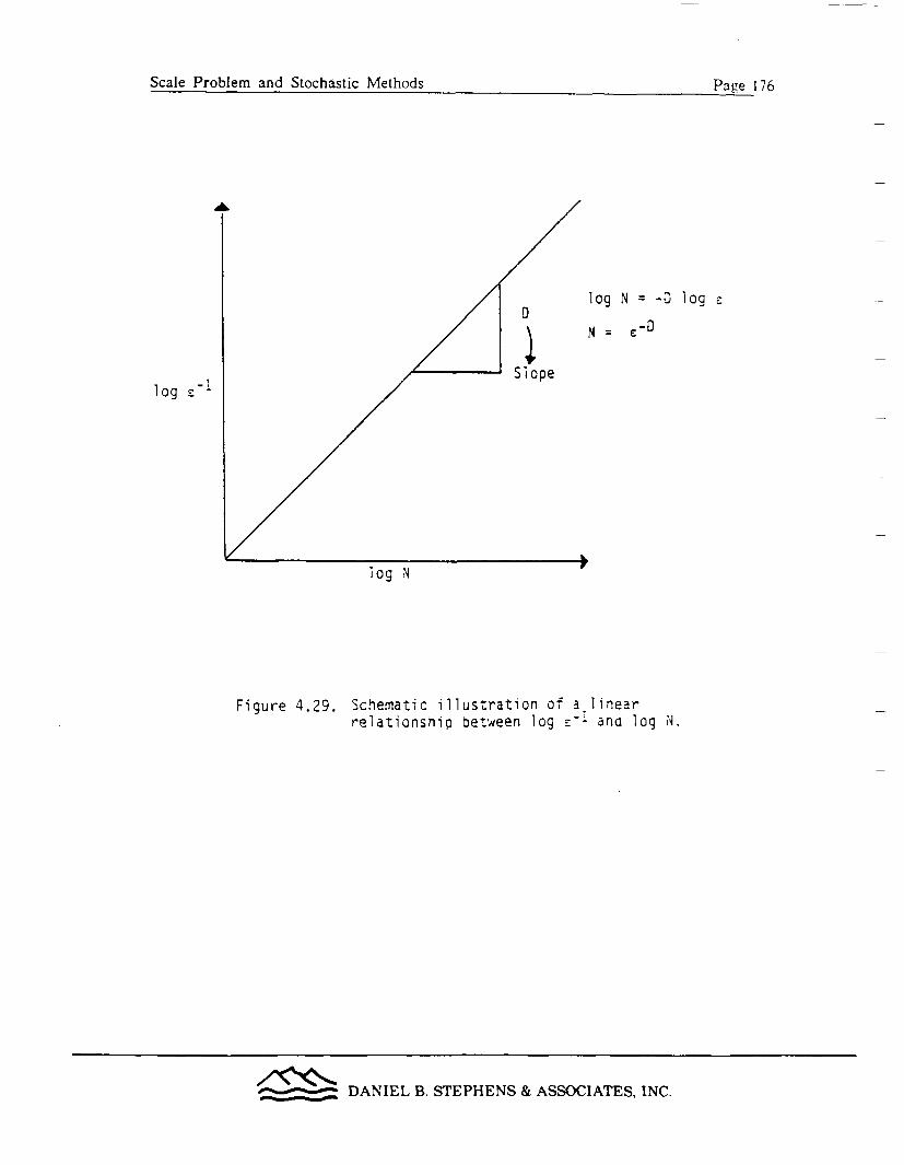
Scale Problem and Stochastic Methods Pace 1 76Scale Problem and Stochastic Methods Paoe ~~7Fc
D
Slope
log N = -D log E
N = e-0
log ^&
Figure 4.29. Schemnatic illustration of a linearrelationship between log :i ana log N.
DANIEL B. STEPHENS & ASSOCIATES, INC.
Scale Problem and Stochastic Methods Pilze 177
we can show that F is always a constant (F = ;D), no matter which scale of
measurement is used. Thus, with the aid of the fractal dimension. we can properly
scale the topographical variation at any scale to any measurement scale. if the
variation is fractal, i.e. self-similar. The length of the distance between two points
L(e) at any measurement scale is then given as:
L(e) - F El-D (4.3.40)
Equation (4.3.40) implies that as long as the distance between two points measured at
a scale. e. and the fractal dimension are known, one can determine the distance
between two points as observed at any other scale. The practical implication of
equation (4.3.40) is tremendous. We can predict large-or small-scale phenomena
based on what we observe at our own measurement scale.
The fractal geometry concept has been recently applied to many scientific
fields (Mandelbrot, 1967; Burrough, 1983a and b; Arya et al., 1985; Hewett. 19S6)
including groundwater hydrology (Wheatcraft and Tyler, 1988). Groundwater
hydrologists, in general, rely on small-scale tests to obtain parameters for predicting
flow or transport phenomena in large-scale geologic formations. Due to the spatial
variability of the parameters, it is generally agreed that it is impractical to delineate
the detailed spatial distribution of the hydrologic parameters in a deterministic sense.
The alternative is to use effective, or mean parameters. This method is, however,
not immune from difficulties. For example, there is field evidence showing that
dispersivity, which is an effective parameter (see section 2.6.1). grows with the scale
of experiment (Gelhar. 1986). So, how can dispersivity values obtained from small-
scale laboratory experiments be scaled to large-scale problems?
To answer the above question, Wheatcraft and Tyler (1988) developed fractal
scaling relationships to analyze dispersion in heterogeneous porous media. They
______ DANIEL B. STEPHENS & ASSOCIATES, INC.

Scale Problem and Stochastic Methods P'ag e I 7S
assumed that the path of a particle in a heterogeneous medium has frau[al
characteristics. The actual length a particle travels in a porous medium Xr can ire
related to the straight line distance of the medium, X, as:
Xf 3 EC1D XSD (4. 3.41)
where EC is the fractal cutoff limit to ensure the actual length the particle travels is
finite. The limit could be the smallest REV size. From equation (4.3.41), one can
see that when the length between two points in a porous medium increases, the
length of the actual travel path of a particle increases accordingly. Now, if we
imagine a large-scale aquifer as a collection of many fractal stream tubes, the
variance of the Xr is then given as:
var(Xf) - var (ccl-D XSD) (4.3.42)
where Xs is constant. If we assume that the fractal dimension, D, is constant, then
equation (4.3.42) can be rewritten as:
var(Xf) = Xs2D var(eC I -D) (4.3.43)
Equation (4.3.43) reveals that the variation in fractal length is due to the variation in
the fractal cut-off limit and is related to the scale of the observation XS' The
variance of Xf can be considered as the spread of a plume in space. Then the
macrodispersivity is:
Ax 2 var (ec I-D) Xs eD-I (4.3.44)
_______ DANIEL B. STEPHENS & ASSOCIATES, INC.
Scale Problem and Stochastic Methods Patse 179
This result. if D = 1. is consistent with that derived by Mercado (1967) in which the
macrodispersivity of a perfectly-stratified aquifer is shown to grow linearly with
travel distance. The expression (4.3.44) was also verified by using random walk
models based on deterministic and stochastic fractal generators (Mandelbrot 1983).
Gelhar et al. (1979) arrived at an expression for macrodispersivity that for early
times is equivalent to Mercado's result. but for late times is equivalent to classical
Taylor's dispersion. i.e., a constant dispersivity. The asymptotic approach to a
constant dispersivity with distance predicted by Gelhar et al. (1979), Gelhar and
Axness (1983), and Dagan (1987) is contrary to the fractal concept.
Finally, Wheatcraft and Tyler (1988) concluded that the dispersion model
based on the fractal geometry concepts predicts that the field-measured dispersivity
will be scale-dependent. The strength of the scale-dependence is directly related to
the fractal dimension. They indicated that it is possible to obtain the fractal
dimension from a tracer experiment in which the breakthrough curve is obtained for
at least two travel distances. As long as the fractal dimension remains constant. it is
then possible to predict solute migration at scales larger than the scale of the
experiment in which the fractal dimension and the cutoff limit were obtained.
A direct application of fractal approach to the groundwater travel time
position may be illustrated in the following example. If we agree that the actual
travel path of a volume of groundwater is a fractal and can be adequately described
by equation (4.3.41), i.e.:
X _ e I-D X D
where, Xf is the total length of the tortuous groundwater path between two points
with a straight line distance, Xs. and if one can assume that the velocity, v, of the
groundwater is constant, the groundwater travel time is then given as:
________ DANIEL B. STEPHENS & ASSOCIATES, INC.
Scale Problem and Stochastic Methods Page 1 80
=f I (EQ -D (XD _3 .4 )
where tf is the actual groundwater travel time for the tortuous path between a
straight line distance. XS' If one further assume that a heterogenous aquifer can be
represented by a bundle of such stream paths in a stochastic fashion. the variance in
the arrival of tracer particles may be expressed as:
var(tf) = I Xs-D var[(Ec) 1-D]V
(4.3.46)
The variance in tf may thus represent the possible spreading in the arrival time of
travel particles. This variance could be treated as a measure of uncertainties in
groundwater travel time prediction. Based on the above equation, the variance in
travel times will grow with Xs to the power of 2D and the variance of the fractal
cutoff limit.
The fractal approach seems to be promising. Wheatcraft and Tyler. (198X)
provided a new way of demonstrating the scale-dependent macrodispersion
phenomena. Although, as they stated, considerable work still needs to be done to
develop a more mature theory, there are some fundamental problems associated with
the fractal approach.
One of the fundamental difficulties in the application of the fractal concept
to groundwater hydrology arises from the self-similarity assumption in the fractal
analysis. Self-similarity implies that the variations in hydrologic properties are
similar at all scales. This assumption is a serious one and it still needs to be
verified.
However, there is evidence supporting the self-similar nature of aquifer
properties. An example is the porosity data reported by Hewett (1986). A sequence
______ DANIEL B. STEPHENS & ASSOCIATES. INC.

Scale Problem and Stochastic Methods Pave 181
of 2189 porosity values taken at intervals of 0.5 ft from a density porosity log in a
well through a late Miocene-early Pleistocene sandstone formation (originally deposited
in a deep submarine fan) was analyzed. The results showed that the porosity values
may be correlated over 300 m. Hewett speculated an even larger range for
horizontal correlations given the anisotropic nature of sedimentary formations. Such
a long-range correlation suggests self-similarity in porosity data; the fractal approach
is most suitable to represent the data.
On the other hand, Burrough (1983a, b) examined soil spatial data series in
The Netherlands and the English Midlands that included percentage of clay, silt, pH,
thickness. soil moisture capacity and topographic height. He concluded that soil does
not vary exactly as an 'ideal' fractal but variation of physical properties is controlled
by many independent processes that can cause abrupt transitions. Thus. soil does not
possess the property of self-similarity at all scales. The spatial variation of soil
properties is suggested to be a result of several closely spaced, nested scales of
variation, occurring over short distances. He concluded that the geostatistical
approach seems to be more appropriate than fractal analysis.
In groundwater transport cases, one may assume that the actual flow path of
a particle in porous media is a fractal, as Wheatcraft and Tyler (1988) did.
However, proving the validity of the assumption may be possible, but difficult. At
present, we are somewhat skeptical of its validity. In fact, many stochastic analyses
of dispersion in heterogeneous media (Gelhar et al., 1979; Gelhar and Axness, 1983;
Dagan, 1987) showed that scale-dependent dispersion may exist only at early times of
a transport process. An asymptotic dispersivity will develop after the plume is
displaced at distances larger than the correlation scales of the hydraulic conductivity
of media.
Results of the stochastic analyses by Gelhar and Axness (1983) and Dagan
(1987) have been tested recently with carefully-designed large-scale field experiments
_______ DANIEL B. STEPHENS & ASSOCIATES, INC.
Scale Problem and Stochastic Methods Page 1S2
by Sudicky (1986). Freyberg (1986), and Garabedian (1987). Asymlptotic
macrodispersivities indeed occurred in these field experiments shortly after the
injection of tracers. They all concluded that stochastic results by Gelhar and Axness
(1983) and Dagan (1987) are robust and are in good agreement with field data.
Although the robustness of the stochastic results may remain to be tested with many
more large field experiments conducted at various geologic environments, it seems that
continuously-growing dispersivity as predicted by the fractal approach may not exist,
at least at a practical range of the size of aquifer. In fact, the boundless dispersivity
predicted by the fractal analysis may arise from the fundamental assumption in the
fractal approach which states that the variations in groundwater particle travel path
are self-similar at all scales.
Regardless of whether the variation in flow channels in porous media (or the
variation in intrinsic permeability which is determined by pore structure) is self-
similar at all scales, the movement of the particles may not be self-similar. This is
because the flow path of groundwater is also controlled by many other factors such
as gradients, density variations, temperature variations, chemical variations, and
degree of saturation under variable saturated flow conditions. Due to the influences
of these factors, the travel path of a particle in the aquifer may likely be non-fractal,
even if the pore channel is fractal. Theoretical analysis by Matheron and de Marsily
(1980) seemed to demonstrate this conjecture. They showed that asymptotic
macrodispersivity may develop at distances much less than the correlation scale of the
hydraulic conductivity field if the flow is not parallel to the bedding. This results in
an extra mixing effect and accelerates the development of an asymptotic
macrodispersivity. This implies that the travel path no longer possesses the self-
similar nature in properties of geologic formations. Deterministic numerical
simulations of effects of heterogeneities on dispersion by Gannon and Yeh (1988)
showed similar results. Hence. if the dispersivity depends on factors other than the
________ DANIEL B. STEPHENS & ASSOCIATES, INC.
Scale Problem and Stochastic Methods Page 1S3
structure of porous media (which could be a fractal but needs to be proved). the
fractal approach may face a formidable task as far as practical application is
concerned.
Furthermore, it will be equally difficult to relate the parameters (such as
fractal cutoff limit and fractal dimension) in Wheatcraft and Tyler's model to
measurable physical parameters (such as hydraulic conductivity or porosity). This
relationship needs to be explored.
________DANIEL B. STEPHENS & ASSOCIATES, INC.
Scale Problem and Stochastic Methods P.t!e IS4
5.0 SUMMARY AND CONCLUSION
There appears to be a fundamental problem with the NRC performance
objectives for High Level Waste repositories, or "groundwater travel time (G\\TT)
objective" . which is stated in 10 CFR 60.113 (a)(2) as "...groundwater travel time
along the fastest path of likely radionuclide travel from the disturbed zone to the
accessible environment shall be at least 1000 years or such other time as may be
approved or specified by the Commission." The "groundwater travel time along the
fastest path" stated in the GW1T objective is an ambiguous phrase. The fastest path
which groundwater travels can never be clearly defined because of the scale problem
in groundwater hydrology. To circumvent this problem, the travel time of a certain
concentration level of radionuclide should be used. The radionuclide or tracer would
be a hypothetical release to the accessible environment which would travel under
pre-waste emplacement hydrogeologic conditions. A concentration based standard is
preferred because of the fact that the concentration represents the total mass flux (or
total mass of newly-arrived groundwater) in a volume, resulting from flow
phenomena of various scales. With this revised definition, a convection-dispersion
equation can then be used to properly determine the arrival of the critical
hyphotetical radionuclide or tracer concentration level. This approach overcomes the
concern for data needed to compute the travel time for a particular molecule of
radionuclide to arrive at the accesible environment. Unless this problem is resolved,
the GWTT objectives will not be met.
In addition to the ambiguity of the GWTT objectives discussed above, there
is another area of difficulty. Determining groundwater travel times and paths in a
regional-scale problem is a difficult task based on the current monitoring and
modeling techniques. There are large uncertainties in predictions. These
uncertainties arise from many sources including those discussed previously. It is,
_______ DANIEL B. STEPHENS & ASSOCIATES, INC.

Scale Problem and Stochastic Methods Page I S5
however, generally agreed that lack of complete knowledge of the spatial distribution
of hydrologic parameters input to a mathematical models may be the major sourze of
uncertainties in predicting the travel times and paths. Means of acquiring more
detailed knowledge of the parameter distributions will certainly improve our
predictive capability. However, such techniques may not exist in the foreseeable
future unless there are some technological breakthroughs in field testing. Until then.
we may have to rely on stochastic approaches to obtain probabilistic results. Many
of these approaches are available including fractal geometry techniques,
macrodispersion methods, Monte Carlo approaches, and conditional simulation. Each
of these methods has limitations. Nevertheless, these approaches may at least provide
us with some estimates of uncertainties in the predictions which may be crucial for
regulatory and decision-making purposes. One should, however. bear in mind that
the uncertainty estimates afforded by the stochastic models are themselves uncertain.
The fractal approach recognizes the existence of variability in all scales but
assumes these variations are self-similar. With these assumptions. one can scale the
results of experiments made at one scale to another. This approach is an easy way
to estimate the uncertainty in groundwater travel times as indicated by equation
(4.3.46). However, in this approach, the parameters lack physical meaning. What
does the fractal dimension, D. mean? How can D and Ec be related to the parameters
(such as hydraulic conductivity, porosity, and their spatial variability) in the classic
groundwater hydrology? More importantly, can we define clearly the volume of
groundwater which we use to define the velocity? The tracer concentration of a
volume of groundwater may be subject to changes due to mixing from subscale
variations in groundwater velocity. Are we interested in the arrival of a volume of
groundwater or a certain concentration of groundwater? Finally, the question which
was posed in the section dealing with the fractal concept must be answered: is it
true that the groundwater travel path is a fractal? Until these questions can be
_______ DANIEL B. STEPHENS & ASSOCIATES, INC.

Scale Problem and Stochastic Methods Page I S6
resolved, the application of the fractal approach must be limited.
The approach using effective parameters with the macrodispersion concert
may be attractive for relatively simple hydrogeologic systems. Recent field
experiments (Sudicky, 1986; Freyberg. 1986; and Garabedian. 1987) show that mean
travel times and paths of plumes in sandy and glacial outwash aquifers can be
adequately predicted by the effective hydraulic conductivity formula developed by
Gelhar and Axness (1983).
The spatial concentration variances are also in reasonable agreement with the
stochastic results by Gelhar and Axness (1983) and Dagan (1987). However, the major
concern with this effective parameter approach is its validity in analysis of flow and
transport in highly heterogeneous aquifers where the variance of log saturated
hydraulic conductivity is greater than 1. The variance of log saturated hydraulic
conductivity in all the possible radioactive waste repository sites is likely much
greater than 1. especially in fractured aquifers. The existing analytical solutions to
stochastic differential equations are also only useful for simple flow fields, e.g.,
steady, uniform flow in a single aquifer. These stochastic results based on an
analytical approach may serve as a tool for preliminary analyses but are not
completely adequate for predictive purposes because of large variance associated with
the results.
Furthermore, the spatial concentration variance formulas in the stochastic
results (equations 4.3.33 to 4.3.36) provide us with the way to predict only the
relative size of the plume. The shape of the concentration profile still remains
unknown. The macrodispersivity defined in the stochastic analysis does not warrant
the use of the classic convection-dispersion equation (Yeh, 1987) based on Fick's law.
In addition, the variance of the predicted mean concentration profile may be large
(Dagan, 1987). Most importantly. the number of samples required to obtain accurate
estimates of the parameter values (correlation scales and covariance functions) for the
________ DANIEL B. STEPHENS & ASSOCIATES, INC.
Scale Problem and Stochastic Methods Pagge 187
macrodispersivity models still must be investigated. Finally, the stochastic results
need to be tested with many large-scale field tracer experiments in various geologic
environments before they can be used for predictions.
Although the Monte Carlo simulation technique may be expensive because it
requires a large number of simulations, it may be the most powerful tool among the
available techniques for predicting groundwater travel times and paths or the arrival
of the radionuclide concentration. Furthermore, conditional simulations which use
available information at sample locations will enhance our ability to model the reality.
Although the results of conditional simulations by Delhomme (1979) indicated that
using the known transmissivity values at sample locations may not reduce the
uncertainties in the prediction of groundwater hydraulic heads significantly, he
suggested that using both hydraulic head information and transmissivity values as
constraints for the simulation may be useful. In addition, the results of the
conditional simulations by Smith and Schwartz (1981) showed that the locations of the
sample data used in the conditional simulation may have important impacts on the
reduction of uncertainties. The effects of sample locations and conditioning the
simulations by hydraulic conductivity, hydraulic head, and porosity values on
predicting uncertainties in groundwater travel times and paths certainly deserves
further investigation. Regardless of the amount of uncertainties that the conditional
simulations (using both conductivity and head values) can reduce, it is rational to
include all the available parameter values in the prediction. It is clear that the
uncertainty in the simulation will be gradually reduced as more and more data
become available. Thus, the conditional simulation seems to be the only tool that
could bring us a step closer to reality.
As one approach to the problem of quantifying uncertainty in groundwater
travel times and paths in porous media using stochastic methods, we suggest the
following steps: (I) groundwater hydrologists should utilize the principles of structural
_______ DANIEL B. STEPHENS & ASSOCIATES, INC.
Scale Problem and Stochastic Methods l~a~e lSS
geology, stratigraphy, and sedimentology to delineate large-scale geologic units or
structures which may contain the likely fast paths along wt hich groundwater travels
(Williams, 1988). (2) "Enough" data should be collected to characterize hydrologic
properties of as many geologic units as possible so that the general flow regime in
those units can be defined. (3) An "intensive" sampling program should be carried
out to collect hydraulic conductivity, dispersivity, porosity data from the geologic
units identified in (1) using many small-scale tests (such as core samples from
boreholes, or small-scale aquifer tests). (4) Groundwater hydrology modelers should
characterize the spatial variability of the hydrologic parameters in the likely fast flow
units by the stochastic concept (i.e., statistical distributions, spatial covariance
functions, etc.). (5) With the calculated statistics for the hydrological parameters. one
should use the effective parameter approaches (such as Gelhar and Axness, 1983; and
Dagan, 1987) for a preliminary analysis to define the mean behavior of the flow
system or to calibrate flow models (see discussion in Section 4.3 or example in
Gelhar, 1986). Note that the scale of samples should be consistent. That is, if one
decides to use a certain scale, the entire characterization program should use that
scale. Thus, the results of the calibration of models may provide a way to have a
better estimate of the statistical parameters required for conditional simulations. (6)
To complement the effective parameter approach, the inverse procedure developed by
Kitanidis and Vomvoris (1983), and Hoeksema and Kitanidis (1984) which uses both
hydraulic conductivity and head data to estimate the spatial covariance function of
the hydraulic conductivity field should be used. The results of the inverse procedure
will provide us with proper input parameter values for the conditional simulation.
(7) Finally, with the available statistical parameters obtained from either the effective
parameter approach or the inverse procedure. one should carry out conditional
simulations using solute transport equations assuming a release of a certain amount of
radionuclides at a disturbed zone to determine the uncertainty in groundwater travel
________ DANIEL B. STEPHENS & ASSOCIATES, INC.
Scale Problem and Stochastic Methods Pai>'e 189
times and paths. As more data become available. the same procedures should le
repeated with the additional data. Such an iterative conditional simulation hwill bring
our predictions close to reality step by step as more hydrologic parameter values are
available. This suggested approach generally concurs with an earlier version of the
NRC's draft generic position on groundwater travel time (Codell. 1986).
On the other hand, if the regulators would accept the mean groundwater
travel time as a measure of the hydrologic integrity of a site, then the convection-
dispersion equation would not be necessary. In this case, the ground water travel
time criterion could be calculated from effective hydraulic properties and the
groundwater flow equation.
Dr. Lynn XV. Gelhar. who is one of the leaders in the field of stochastic
hydrology, received the 0. E. Meinzer Award from the Geological Society of
America in 1987. In concluding this review, it seems appropiate to excerpt some of
his remarks on the current status of stochastic theories and key issues which remain
to be solved.
"We now understand that this heterogeneity plays a central role
regarding the large-scale mixing process in aquifers. The last decade
witnessed a rapid development of mathematical, numerical, and
statistical methodologies for evaluating the effects of heterogeneity on
transport process. In spite of the confusion which seems to still persist
in some recent literature, I believe that it is fair to say that we have
arrived at a sound theoretical description of the dominant field-scale
mixing process. Such stochastic theories provide a framework for
predicting large-scale, long term behavior from observations of aquifer
heterogeneity. Furthermore, such theories provide specific hypotheses
which can be tested systematically by comparing independent
theoretical predictions with the results of controlled field experiments.
DANIEL B. STEPHENS & ASSOCIATES, INC.

Scale Problem and Stochastic Methods Paze 190
This allows us to scape from the circular reasoning of the curve-fitting
approach in ground-water hydrology. The stochastic approach not only
provides a critical link between small-scale laboratory measurments. but
also reveals features of the large-scale process which may not
otherwise be apparent."
.... There is a need for controlled field experiments which explore
more complex transport processes involving chemical heterogeneity,
multi-phase flow, and fractured media. A fractured rock can be
viewed as another type of heterogeneous medium which I suspect can
be treated in some cases using stochastic continuum theory. Clearly.
the problem of solute transport in fractured media is unresolved.
Oversimplified matrix diffusion-type models have been extensively
exercised using hyphotetical parameters to illustrate significant
radionuclide retardation in the context of radioactive-waste disposal.
As far as I can determine, there is no definitive field evidence which
demonstrates such retardation effects. There is an obvious need for
carefully designed field experiments to explore transport processes in
fractured rock. Why aren't experiments of this type being developed
in the United States?
A key unresolved issue is how we can characterize heterogeneity in
practical sense. Research has shown that variances and correlation
scales can be estimated using thousands of samples but our experience
indicates that parameters can be estimated crudely from indirect
geologic and geophysical observations and simple hydraulic tests. This
more practical approach needs to be pursued in a number of different
geologic environments. Heterogeneity remains a formidable difficulty
in hydrogeology. but we now have a quantitative basis for evaluating
_______ DANIEL B. STEPHENS & ASSOCIATES. INC.
Scale Problem and Stochastic Methods
its effects." Gelhar (1988).
Pave 191
_____ DANIEL B. STEPHENS & ASSOCIATES, INC.
Scale Problem and Stochastic Methods P'ahe I192
REFERENCES
Ababou, R. and L.W. Gelhar. Three-dimensional groundwater flow in random media:Direct simulation versus spectral theory, EOS. 68(44). Nov. 3, 1987.
Andersson, J. and A.M. Shapiro, Stochastic analysis of one-dimensional steady stateunsaturated flow: a comparison of Monte Carlo and perturbation methods,Water Resour. Res., 19(1), 121 133. 1983.
Arya. A., T.A. Hewett. R. Larson. and L.W. Lake, Dispersion and reservoirheterogeneity. Society of Petroleum Engineers. SPE14364. Presented at the60th Annual Technical Conference of the Society of Petroleum Engineers,Las Vegas, Nevada. Sept. 22-25, 1985.
Bakr. A.A., Stochastic analysis of the effect of spatial variations in hydraulicconductivity on groundwater flow, Ph.D. dissertation, Newv Mexico Instituteof Mining and Technology, Socorro, July, 1976.
Bakr. A.A., L.W. Gelhar, A.L. Gutjahr. and J.R. MacMillan, Stochastic analysis ofspatial variability in subsurface flows, I:Comparison of one-dimensionalflows, Water Resour. Res..14, 263-271, 1978.
Barrenblat, G.E.. I.P. Zheltov, and J.N. Kochina, Basic Concepts in the theory ofhomogeneous liquids in fissured rocks, J. Appl. Math. Mech. USSR, 24(5): 1286-1303. 1960.
Bear, J., Hydraulics of Groundwater. 569 pp., McGraw-Hill, New York, 1979.
Bennion, D.W.. and J.C. Griffiths, A stochastic model for predicting variations inreservoir rock properties, Trans. AIME, No. 237. Part 2, 9-16, 1966,
Betson, R.P., J.M. Boggs, S.C. Young, L.W. Gelhar, Design of a field experiment toinvestigate groundwater saturated zone transport processes, Interim Rep.,RP2485-05, lO4pp.. Elecr. Power, Res. Inst., Palo Alto, CA, 1985.
Bibby, R., and D.K. Sunada, Statistical error analysis of a numerical model ofconfined groundwater flow, in C.L. Chiu (ed.), Stochastic hydraulics,Proceedings, First International Symposium on Stochastic Hydraulics,591-612. 1971.
Bonano, E.J., and R.M. Cranwell, Treatment of uncertainties in the performanceassessment of geologic high-level radioactive waste repositories, Math. Geol.,20(5), 543-565. 1988.
Bras. R.L., and 1. Rodriguez-lturbe, Random functions and hydrology, Addison-Wesley publishing company, 559pp., 1985.
Bulnes. A.C.. An application of statistical methods to core analysis data of dolomiticlimestone, Trans. AIME, 165, 223-240, 1946.
Burrough, P.A., Multiscale sources of spatial variation in soil. 1: The application offractal concepts to nested levels of soil variation, J. Soil Science. 34.577-597, 1983a.
______ DANIEL B. STEPHENS & ASSOCIATES, INC.
Scale Problem and Stochastic Methods Pavze 193Scale Problem and Stochastic Methods Pai.!e 193~~~~~~~~~~
Burrough, P.A., Multiscale sources of spatial variation in soil, 11: A non-Brownianfractal model and its application in soil survey. J. Soil Science. 34. 599-620.1983b.
Butler, Jr., J.J., Pumping tests in nonuniform aquifers: a deterministic/stochasticanalysis, Ph.D. dissertation, Stanford University, Stanford. CA.. 220 pp..December 1986.
Byers, E. and D.B. Stephens. Statistical and stochastic analysis of hydraulicconductivity and particle size in a fluivial sand. Soil Sci Soc. Am. J. 47.1072-1081, 1983.
Clifton, P.M.. and S.P. Neuman, Effects of kriging and inverse modeling onconditional simulation of the Avra Valley aquifer in southern Arizona.Water Resour. Res., 18, 1215-1234, 1982.
Clifton. P.M., B. Sagar, and R.G. Baca. Stochastic groundwater traveltimie modelingusing a Monte Carlo technique, In International Association ofHydrogeologists Memoires: Hydrogeology of Rocks of Low Permeability.Tucson, Arizona. 17(1), 319-329. 1985.
Codell, R., Draft generic position on groundwater travel time. Div. of Waste Nlanag..Office of Nuclear Material Safety and Safeguards. U.S. Nuclear RegulatoryCommisssion, June 30. 1986.
Cole, C.R. and H.P. Foote, Use of a multigrid technique to study effects of limitedsampling of heterogeneity on transport prediction. Presented at the NationalWater Well Association Conference. Solving Ground Water Problenis withModels, Denver, Colorado, February 10-12, 1987.
Csanady, G.T., Turbulent diffusion in the environment, D. Reidel Publishing Co.. 2'48pp., 1973.
Dagan, G.. Solute transport in heterogeneous porous formation, J. Fluid Mech., 145.151-177. 1984.
Dagan, G., Statistical theory of groundwater flow and transport: pore-to laboratory-,laboratory-to formation-and formation-to regional-scale. Water Resour. Res..22(9), 120S-134S. 1986.
Dagan, G., Theory of solute transport by groundwater, Ann. Rev. Fluid Mech.. 19,183-215. 1987.
Davis, J.C., Statistics and Data Analysis in Geology, 550 pp., John Wiley and Sons,Inc., New York, 1973.
Delhomme, J.P., Spatial variability and uncertainty in groundwater flow parameters:a geostatistical approach. Water Resour. Res., 15. 269-280, 1979.
De Marsily, G., G. Lavedan. M. Boucher, G. Fasamino, Interpretation of interferencetests in a well field using geostatistical techniques to fit the permeabilitydistribution in a reservoir model. "in" 0. Verly etal (eds) Geostatistics forNatual Resources Characterization. Part 2. NATO Adv. Sci. Inst. Series C.vol 122, pp 831-849. Reidel Publ, Co., Dordrecht, 1984.
_______ DANIEL B. STEPHENS & ASSOCIATES, INC.
Scale Problem and Stochastic Methods Pmage 194
De Marsily, G.. Quantitative Hydrogeology: Groundwater Hydrogeology for Engineers,440 pp., Academic Press. Inc., Orlando. Florida, 1986.
Dooge. J.C.L.. Scale problems in hydrology. Kisiel Memorial Lecture at Department ofHydrology and Water Resources. University of Arizona. Tucson. Arizona.February 19, 1986.
Driscoll, F.G., Groundwater and Wells. 1089 pp., Johnson Division, St. Paul.Minnesota., 1986.
Elsworth, D., A boundary element-finite element procedure for porous and fracturedmedia flow, Water Resour. Res., 23(4), 551-560, 1987.
Fischer, H.B.,E.J. List. R.C.Y. Koh. J. Imberger, N.H. Brooks, Mixing in inland andcoastal waters. Academic press, 483 pp., 1979.
Freeze, R.A., Three-dimensional, transient, saturated-unsaturated flow in agoundwater basin, Water Resour. Res., 7(2), 347-366, 1971.
Freeze, R.A.. A stochastic-conceptual analysis of one-dimensional groundwater flowin non-uniform homogeneous media, Water Resour. Res.. 725-741, 1975.
Freyberg, D.L., A natural gradient experiment of solute transport in a sand aquifer 2.Spatial moments and the advection and dispersion of nonreactive tracers.Water Resour. Res., 22, 2031-2046, 1986.
Cannon, J. M., and T.-C.J. Yeh, Numerical analysis of the effects of heterogeneitieson dispersion. in prep., 1988.
Garabedian. S.P., Large-scale dispersive transport in aquifers: field experiments andreactive transport theory, PhD. dissertation, Massachusetts Institute ofTechnology, Cambridge, Massachusetts, July 1987.
Gelhar, L.W.. Effects of hydraulic conductivity variations on groundwater flows, inProceedings of the second interational IAHR symposium on stochastichydraulic, Int. Ass. of Hydraul. Res., Lund, Sweden, 1976.
Gelhar, L.W., Stochastic subsurface hydrology from theory to applications. WaterResour. Res., 135S-145S, 1986.
Gelhar, L.W. and C.L. Axness, Three-dimensional stochastic analysis ofmacrodispersion in aquifers, Water Resour. Res., 19(l). 161-180, 1983.
Gelhar. L.W., A.A. Bakr, A.L. Gutjahr, and J.R. McMillan, Comments on stochasticconceptual analysis of one-dimensional groundwater flow in a non-unifromhomogeneous medium by Freeze, R.A., Water Resour. Res. 13(2), 477-480,1977.
Gelhar, L.W., A.L. Gutjahr, and R.L. Naff, Stochastic analysis of macrodispersionin a stratified aquifer. Water Resour. Res., 15, 1387-1397, 1979.
Gelhar. L.W., Response to O.E. Meinzer Award. GSA Bulletin, July, P984, 1988.
Gutjahr, A.L., Kriging in stochastic hydrology: Assessing the worth of data, paper
________ DANIEL B. STEPHENS & ASSOCIATES, INC.
Scale Problem and Stochastic Methods Pace 195
presented at the Chapman Conference on Spatial Variability in HydrologicModeling, AGU. Fort Collins, Colorado., July 198.
Gutjahr, A.L., L.W. Gelhar, A.A. Bakr, and J.R. MacMillan, Stochastic analysis ofspatial variability in subsurface flows, 2: Evaluation and Applications,Water Resour. Res., 14, 953-960, 1978.
Gutjahr. A.L., D. McKay. and J.L. Wilson, Fast Fourier transform methods forrandom field generation, EOS, 68(44), Nov. 3, 1987.
Heller, J.P., Observations on diffusion and mixing in porous media, in Proceedings,Second International Symposium on Fundamentals of Transport Phenomenain Porous Media, IAHR and ISSS, Vol. 1, Guelph, University of Guelph,1-26, 1972.
Hewett, T.A., Fractal distributions of reservoir heterogeneity and their influence onfluid transport, Society of Petroleum Engineers. SPE15386. Presented at the61st Annual Technical Conference of the Society of Petroleum Engineers,New Orlans, Louisiana, October 5-8, 1986.
Hoeksema, R.J. and P.K. Kitanidis, An application of the geostatistical approach tothe inverse problem in two-dimensional groundwater modeling, WaterResour. Res, 20(7), 1003-1020, 1984.
Hoeksema, R.J. and P.K. Kitanidis, Analysis of the spatial structure of properties ofselected aquifers, Water Resour. Res, 21, 563-572. 1985.
Huang, C. and D.D. Evans, A 3-dimensional computer model to simulate fluid flowand contaminant transport through a rock fracture system, NUREG/CR-4042, U.S. Nuclear Regulatory Commission, 108 pp., 1985.
Hubbert, M.K., The theory of groundwater motion, J. of Geol., 48, 785-944, 1940.
Huyakorn, P.S., B.H. Lester, and C.R. Faust, Finite element techniques of modelinggroundwater flow in fractured aquifers, Water Resour. Res., 19(4),1019-1035, 1983a.
Huyakorn, P.S., B.H. Lester, and J.W. Mercer, An efficient finite element techniquefor modeling transport in fractured porous media, 1, Single SpeciesTransport, Water Resour. Res., 19(3):841-854, 1983b.
Huyakorn, P.S., B.H. Lester and J.W. Mercer, An efficent finite element techniquefor modeling transport in fractured porous media, 2, Nuclide decay chaintransport, Water Resour. Res., 19(3). 841-854, 1983c.
Ilyin, N.I., and others, Otsenka tochnosti opredeleniya vodopronitsayemosti gornykhporod, Moscow, Nedra, 1971.
Javandel, I., and P.A., Witherspoon, A method of analyzing transient fluid flow inmultilayered aquifers, Water Resour. Res., 5(4), 1969.
Jenkins. G.M. and D.G. Watts. Spectral Analysis and its Applications. 525 pp..Holden-Day, Inc., San Francisco. 1968.
DANIEL B. STEPHENS & ASSOCIATES, INC.

Scale Problem and Stochastic Methods Page 196
Jensen. J.L., D.V. Hinkley. L.W. Lake, A statistical study of reservoir pernleallility:distribution, correlation and averages, Soc. Petr. Eng. Formation Evaluation.461-468, Dec. 1987.
Journel, A.G., and CH.J. Huijbregts. 600 pp., Mining Geostatistics. Acadenmic Press.London, 1978.
Kazemi, H., M.S. Seth, and G.W. Thomas, The interpretation of interference tests innaturally fractured reservoirs with uniform fracture distribution. Soc. Pet.Eng. J., Dec., 463-472, 1969,
Kitanidis. P.K., and E.G. Vomvoris, A geostatistical approach to the inverse problemin groundwater modeliling (steady-state) and one-dimensional simulations.Water Resour. Res., 19(3), 677-690, 1983.
Law, J., A statistical approach to the interstitial heterogeneity of sand reservoirs,Trans AIME, v. 155, 202-222, 1944.
Lumley, J.L., and H.A. Panofsky, The Structure of Atmospheric Turbulence, JohnWiley, New York, 1964.
MacMillan, J.R. and A.L., Gutjahr, Geological controls on spatial variability for one-dimensional arrays of porosity and permeability normal to layering, inReservoir Characterization, edit by Haldorsen and Lake, 256-291, AcademicPress, 1986.
Mandelbrot, B.B., The Fractal Geometry of Nature. 468 pp., W.H. Freeman, SanFrancisco, California, 1983.
Mandelbrot, B.B., How long is the coastline of Great Britain? Statistical self-similarityand fractional dimension, Science, 155, 636-638, 1967.
Mantoglou, A., and L.W. Gelhar, Stochastic modeling of large-scale transientunsaturated flow systems, Water Resour, Res., 23(1), 37-46, 1987a.
Mantoglou, A., and L.W. Gelhar, Capillary tension head variance, mean soil moistsurecontent, and effctive specific soil moisture capacity of transientunsaturated flow in stratified soils, Water Resour. Res., 23(1), 47-56, 1987b.
Mantoglou, A. and L.W. Gelhar, Effective hydraulic conductivities of transientunsaturated flow in stratified soils, Water Resour. Res., 23(1), 57-68, 1987c.
Mantoglou. A., and J.L. Wilson, The turning bands method for simulation of randomfields using line generation by a spectral method, Water Resour. Res., 18(5).1379-1394, 1982.
Marle, C., Ecoulements polyphasiques en milieu poreux, Rev. Inst. Fr. Pet, 22(10),1471-1509, 1967.
Matheron. G.. The intrinsic random functions and their applications, Advan. Appl.Probab., 5. 438-468, 1973.
Matheron, G., and G. de Marsily. Is transport in porous media always diffusive? Aconunter example, Water Resour. Res., 16(5), 901-917, 1980.
________DANIEL B. STEPHENS & ASSOCIATES, INC.

Scale Problem and Stochastic Methods Page 197Scale Problem and Stochastic Methods Pace 197
Mercado, A., The spreading pattern of injected water in a permeability-straftiiedaquifer. p. 23, Proc. Int. Assoc. Sci. Hydrol. Svrmp.. Haifa Pub. 72. 1967.
Mizell, S.A., A.L. Gutjahr, and L.W. Gelhar, Stochastic analysis of spatial variabilityin two-dimensional steady groundwater flow assuming stationary and non-stationary heads, Water Resour. Res., 19. 1853-IS67, 1982.
Moench, A.F., Double-porosity models for a fissured groundwater reservoir withfracture skin, Water Resour. Res.. 20(7), 831-846, 1984.
Morrison, P., and P. Morrison, Powers of Ten. Scientific American Books, New York.1982.
Neuman, S.P., Stochastic continuum representation of fractured rock permeability asan alternative to the REV and fracture network concepts, 533-561, 28thU.S. symposium on rock mechanics, Tucson, Arizona, 29 June -I July,1987.
Neuman, S.P., Role of geostatistics in subsurface hydrology, in G. Verly, M. David,A.G. Journel. and A. Marechal, eds., Geostatistics for Natural ResourcesCharacterization, Part 2, p787-816. D. Roede, Publ. Co.. Boston. MA, 1072pp., 1984.
Neuman, S.P., C.L. Winter, and C.M. Newman, Stochastic theory of field-scaleFickian dispersion in anisotropic porous media, Water Resour. Res., 23,453-466, 1987.
Neuman, S.P., Statistical Characterization of aquifer heterogeneities, in Recent Trendsin Hydrogeology, Geol. Soc. Amer. Spec. Paper 189, 81-102, 1982.
Parsons, A.M., E.D. Mattson, D.B. Stephens. K. Flanigan. K. Black, Field simulation ofwaste impoundment seepage in the vadoze zone, Proc. Flows onSouthwestern Groundwater Issues Conf., Nat. Water Well Assoc.,Albuquerque, March 23-25, 1988.
Peters, R.R., J.H. Gauthier, and A.L. Dudley, The effect of percolation rate onwater-travel time in deep, partially saturated zones, Sandia Report.SAND85-0854, 1986.
Rasmussen, T.C.. Computer simulation of steady fluid flow and solute transportthrough three-dimensional networks of variably saturated, discrete fractures,in Evans, D.D. and T.J. Nicholson (Eds.), Flow and Transport ThroughUnsaturated Fractured Rock, AGU Geophysical Monograph 42, 107-114,1987.
Schwartz, F.W., L. Smith, and A.S. Crowe, 1983. A stochastic analysis ofmacroscopic dispersion in fractured media, Water Resour. Res..19,1253-1265, 1983.
Shapiro. A. M., and J. Andersson, Steady-state fluid reposnes in fractured rock: Aboundary element solution for a coupled, discrete fracture continuum model,Water Resour. Res. 19(4), 959-969, 1983.
Smith, L., and R.A. Freeze, Stochastic analysis of steady state groundwater flow in
DANIEL B. STEPHENS & ASSOCIATES, INC.
Scale Problem and Stochastic Methods Pagze 198
a bounded domain, 1: One-dimensional simulations. Water Resour. Res.. 15.521-528, 1979a.
Smith, L.. and R.A. Freeze. Stochastic analysis of steady state groundwater flo\v in abounded domain. 2: Two-dimensional simulations, WNater Resour. Res.. 15.1543-1559, 1979b.
Smith, L. and F.W. Schwartz, Mass transport. 1. A stochastic analysis of macroscopicdispersion, Water Resour. Res., 16, 303-313, 1980.
Smith, L. and F.W. Schwartz. Mass transport, 2. Analysis of uncertainty inprediction, Water Resour. Res., 17(2), 351-368. 1981a.
Smith. L. and F.W. Schwartz, Mass transport, 3. Role of hydraulic conductivity inprediction, Water Resour. Res.. 17(5). 1463-1479. 1981b.
Stephens. D.B.. L.W. Gelhar, S. Young, Field experiment to evaluate disperison inunsaturated media, EOS, 65(16). 106, 1984.
Sudicky, E.A., A natural gradient experiment on solute transport in a sand aquifer:spatial variability of hydraulic conductivity and its role in the dispersionprocess. Water Resour. Res.. 22, 2069-2082, 1986.
Taylor, G.1.. Diffusion by continuous movements, Proc. London. Math. Soc. Ser. A20.196-211. 1922.
Taylor, G.I., Dispersion of soluble matter in solvent flowing slowly through a tube.Proc. London. Math. Soc. Ser. A219. 186-203, 1953.
van Genuchten, M.T., A closed-form equation for predicting the hydraulicconductivity of unsaturated soils, Soil Sci. Soc. Am. J., 44, 892-898, 1980.
Vomvoris, E.G.. and L.W. Gelhar, Stochastic prediction of dispersive contaminanttransport, U.S. Department of Commerce National Technical InformationService, Cooperative Agreement, CR-811135-01-2, Dec., 1986.
Wang, J.S.Y., and T.N. Narasimhan, Hydrologic mechanisms governing fluid flow ina partially saturated, fractured, porous medium, Water Resour. Res.. 21(12).1861-1874, 1985.
Warren, J.E., and H.S. Price, Flow in heterogeneous porous media. Society ofPetroleum Engineers Journal, 1, 153-169. 1961.
Warren, J.E., and P.J. Root, Behavior of naturally fractured reservoirs, Society ofPetroleum Engineers Journal, 9. 245-255. 1963.
Warren. J.E., and F.F. Skiba, Macroscopic dispersion, Trans AIME, 231, 215-230.1964.
Warren, J.E., F.F. Skiba, and H.S. Price. An evaluation of the significance ofpermeability measurements, Journal Petroleum Technology, 13. 739-744,1961.
Wheatcraft, S.W. and S.W. Tyler, An explanation of scale-dependent dispersivity in
_______ DANIEL B. STEPHENS & ASSOCIATES, INC.
Scale Problem and Stochastic Methods P'age 199
heterogeneous aquifers using concepts of fractal geometry. \Water lesour.Res., 24(4), 525-532, 1988.
Wierenga, P.J., L.W. Gelhar, C.S. Simmons. G.W. Gee. T.J. Nicholson. Validation ofstochastic flow and transport models for unsaturated soil: a comprehensivefield study, U.S. Nuc. Reg. Comm. Reprt, NUREG/CR-4622. 1986.
Williams, D., Geostatistical analysis and inverse modeling of the Upper Santa CruzBasin, Arizona, Master Thesis, Univ. of Arizona. pp1 49 , 1987.
Williams, R.E., Comment on "Statistical theory of groundwater flow and transport:Pore to Laboratory, Laboratory to Formation, and Formation to RegionalScale" by Gedeon Dagan, Water Resour. Res., 24(7), 1197-1200. 1988.
Williams, R.E., Comment on "Double-porosity models for a fissured groundwaterreservoir with fracture skin" by Allen F. Moench. Water Resour. Res.,21(6), 889-891, 1985.
Winter, C.L., C.M. Newman, and S.P. Neuman. A perturbation expansion fordiffusion in a random velocity field, SIAM J. Appl. Math, 44(2). 411-424.1984.
Yeh, T.-C.J., L.W. Gelhar and A.L. Gutjahr, Stochastic analysis of unsaturated flowin heterogeneous soils, 1. Statistically isotropic media. Water Resour. Res..21(4), 447-456, 1985a.
Yeh. T.-C.J., L.W. Gelhar and A.L. Gutjahr, Stochastic analysis of unsaturated flowin heterogeneous soils, 2, Statistically anisotropic media with variable alpha,Water Resour. Res., 21(4), 457-464, 1985b.
Yeh, T.-C.J., L.W. Gelhar and A.L. Gutjahr. Stochastic analysis of unsaturated flowin heterogeneous soils, 3, Observations and applications. Water Resour.Res., 21(4), 465-472, 1985c.
Yeh. T.-C.J., Comment on "Modeling of scale-dependent dispersion in hydrogelogicsystems" by J.F. Pickens and G.E. Grisak, Water Resour. Res.. 23(3), 522,1987.
Zhang, Y., Double porocity model and its finite element solution for the flow infractured-Karst Rocks. Hydrogeology and Engineering Geology. 4. 1982.
______ DANIEL B. STEPHENS & ASSOCIATES, INC.

Scale Problem and Stochastic Methods Palse A-\l
APPENDIX A
Glossary
Note that the glossary provided here is intended to clarify the concepts or
physical meanings of terms, instead of rigorous definitions. Although most of the
definitions refer to space series. they can be applied to time series as well.
Autocorrelation function: A function which depicts the linear correlation between a
space series at all ranges of offset distance. For example, an
autocorrelation function of hydraulic conductivity values along a transect
is a measure of the intensity of association or interdependence among the
values at all ranges of separation distances. Syn: autocorrelation,
correlation function.
Autocovariance function: A function which describes the behavior of the covariances
of two identical spatial series offset at various separation distances.
Correlation (correlation coefficient): the ratio of the covariance of two random
variables to the product of their standard deviations. The correlation
coefficient ranges from +1 to -1. A correlation of +1 indicates a perfect
direct relationship between two random variables; a correlation of -I
indicates that one variable changes inversely with relation to the other.
Between the two extremes is a spectrum of less than-perfect relationships,
including a correlation coefficient of zero which indicates the lack of any
linear relationship.
Correlation scale: A separation distance beyond which the random variables are no
_______ DANIEL B. STEPHENS & ASSOCIATES, INC.

Scale Problem and Stochastic Methods Pace A2
longer considered correlated. Physically, it can he related to the average
size of all sedimentary structures (for example. clay lenses) in an aquifer.
Cross-correlation function: A function which describes the correlation between two
different data series at all separation distances. For example. a cross-
correlation function of hydraulic conductivity and head values along a
transect shows the relationship between the conductivity and head values
along the transect at various separation distance. Syn: cross-correlation.
Cross-covariance function: A function which characterizes the covariances of spatial
series of two different properties (e.g., hydraulic conductivity and
porosity) at different separation distances. Syn: cross-covariance.
Co-Kriging: A method for estimating the value of a spatially distributed variable (e.g.
transmissivity) from adjacent values of two variables (such as
transmissivity and well capacity) while considering the spatial
interdependence (cross-covariance) of the two variables.
Conditional probability: The probability of occurrence of a property value at an
unsampled location if the property values at other location are known.
Conditional simulation: A data-generating technique, used with Monte Carlo
simulation. However, sample values at sample locations are preserved in
the generated data by this technique.
Covariance: A measure of the distribution of values of two properties around a
common mean and thus of their mutual variability.
________ DANIEL B. STEPHENS & ASSOCIATES, INC.

Scale Problem and Stochastic Methods Page A 3
Ensemble: A collection of an infinite number of space series measuring the same
variable.
Ensemble average: An average of the property at a point in space over many
possible space series. Syn. expected value.
Ergodicity: A property of a stochastic process which says the ensemble moments
equal the corresponding averages calculated from a single realization.
These averages in turn can be approximated from a finite part of the
realization.
Expected value: see ensemble average.
First moment: see mean
Frequency distribution: A table or a plot which divides a set of data into a number
of classes. and shows the number of data belonging in each class.
Geostatistics: Statistics as applied to geology generally including correlated processes.
In groundwater hydrology. it is the application of random function
concepts to study the hydrologic properties in space.
Integral scale: A convenient measure of autocorrelation of a stochastic process. It
carries the same physical meaning as the correlation scale but is defined
more rigorously. Mathematically, it is defined as the area under the
autocorrelation function.
______ DANIEL B. STEPHENS & ASSOCIATES, INC.
Scale Problem and Stochastic Methods Page A4
Intrinsic hypothesis: A less stringent hypothesis than that of second-order
stationarity. It states that a random field is intrinsic only if the variance
of the increments of the random field is finite and these increments are
second-order stationary. Variogram analysis is then applicable.
Joint probability function: A function which describes the behavior of the joint
probability distribution of many random variables (i.e.. the probabilities of
occurrence of many random variables).
Kriging: A method for estimating the value of a spatially distributed variable from
adjacent values while considering the spatial interdependence of the
variables.
Log hydraulic conductivity: The natural logarithm of a hydraulic conductivity value.
(InK) or the logarithm of a hydraulic conductivity value to the base 10,
(logK).
Log transmissivity: The natural logarithm of a transmissivity value, (InT), or the
logarithm of a transmissivity value to the base 10. (logT).
Lognormal distribution: A frequency distribution whose logarithms follow a normal
distribution.
Mean: The sum of all observations divided by the number of observations.
Median: The value of the middle term in a set of data arranged in rank order.
_______ DANIEL B. STEPHENS & ASSOCIATES, INC.

Scale Problem and Stochastic Methods Pase AS
Mode: The value or group of values that occurs with greatest frequency in a set of
data; the most typical observation.
Monte Carlo simulation: A data-generating technique. It generates large samples of
data from known probability distributions.
Nonstationary process: A stochastic process which does not possess stationary
properties. Generally, it refers to a process which contains a significant
trend or where the covariance depends on location as well as separation
distance.
Normal distribution: A frequency distribution whose plot is a continuous, infinite,
bell-shape curve that is symmetrical about its arithmetic mean, mode. and
median. Syn: Gaussian distribution; bell-shaped distribution.
Nugget effect: A jump exhibited at the origin of a variogram. It generally
represents uncorrelated measurement errors or subscale variability.
Perfectly correlated process: A process which has infinitely large correlation scales.
Generally, this process has a constant value over space.
Probability: A term to describe the frequency of occurrence of an event.
Probability distribution: A distribution of frequencies of occurrence of many events.
It is approximated by a frequency distribution.
Random variable: A function whose values are real numbers and depend on
DANIEL B. STEPHENS & ASSOCIATES, INC.

Scale Problem and Stochastic Methods Page A6
"chance" or probability.
Random field: see stochastic process.
Random function: see stochastic process.
Range: The distance beyond which the value of the variogram equals the variance of
the random field. Similar to the correlation scale, it is the distance
beyond which the interdependence of values in a space series is
considered insignificant.
Realization: A single space series in an ensemble. For example, a set of porosity
values measured in an aquifer is considered as a realization of all the
possible porosity values of the aquifer.
Regionalized variable: A variable which is distributed in space. It is equivalent to a
realization of a stochastic process. Examples are porosity, hydraulic
conductivity, and other hydrologic properties of an aquifer.
Representation theorem: A theorem which allows a second-order stationary stochastic
process to be decomposed into sums of uncorrelated (or orthogonal)
increments in the frequency domain.
Second moment: see variance.
Second-order stationary (weakly stationary) process: A stochastic process in which the
ensemble mean (expected value) of the process is constant over space. and
________ DANIEL B. STEPHENS & ASSOCIATES, INC.
Scale Problem and Stochastic Methods Page A 7
the autocovariance function depends only on the separation distance.
Separation distance: The amount of offset in distance between the two space series
being compared.
Sill: The asymptotic value of a variogram at a separation distance equal to or
greater than the range. It is the variance of the random field.
Spectral Method: A mathematical tool used to solve partial differential equations
which contain stochastic parameters.
Spectrum: The inverse Fourier transform of a covariance function. In other words,
the covariance function has been transformed from a space domain to a
wave number domain.
Standard deviation: Square root of the variance; it describes dispersion or spread of
data around the mean.
Statistical moment: A convenient measure of the location and the shape of a
probability distribution. First, second, and third moments of a probability
distribution correspond to mean, variance, and skewness of the
distribution.
Statistically anisotropic process: A stochastic process in which the covariance function
depends not only on the magnitude of the separation distance but also on
the direction of the separation distance. That is, the correlation scales of
the process varies with change in direction.
_______ DANIEL B. STEPHENS & ASSOCIATES, INC.
Scale Problem and Stochastic Methods Pace AS
Statistically homogeneous process: see second-order stationary process.
Statistically heterogeneous process: Any process that does not possess the properties of
a second-order stationary process.
Statistically isotropic process: A stochastic process in which the covariance function
depends only on the magnitude of the separation distance, regardless of
the direction. That is, the correlation scales of the process are invariant
in all directions.
Statistically independent: Two random variables are statistically independent if and
only if the joint distribution of the two random variables equals the
product of the individual probability distributions of the two random
variables. That is, one random variable conveys no information about the
other random variable.
Stationary process: If the statistical properties of a spatial stochastic process do not
change over the spatial coordinates, then the stochastic process is a
stationary process. Syn. Strictly stationary process.
Stochastic process: A collection of an infinite number of random variables in space.
Variance: The average squared deviations of all possible observations from the
population mean.
Variogram: A plot of the semivariance of a random field versus separation distances.
Like a covariance function, a variogram is used to define the spatial
DANIEL B. STEPHENS & ASSOCIATES, INC.
Scale Problem and Stochastic Methods Pacte A9
interdependence of two random variables. However. variogram is not
restricted to only stationary or second-order stationary process.
_______ DANIEL B. STEPHENS & ASSOCIATES, INC.
Scale Problem and Stochastic Methods Pace B I
APPENDIX B
B.l Inconsistency in the Development of Governing Groundwater Flow Equations
The purpose of this appendix is to clarify some confusions in the
development of governing groundwater flow equation in saturated porous media.
Therefore, some of the inconsistencies in the derivation will be discussed.
To derive the governing groundwater flow equation, we start with the mass
balance equation. Consider the mass balance of a stationary control volume, VT
(Figure 2.4) whose shape is fixed in space and time. The principle of mass
conservation states that
{ rate of mass accumulation } { rate of mass in - { rate of mass out } (B.l)
To apply the principle to the control volume, we begin by considering the pair of
faces perpendicular to the x axis. The rate of mass in through the face at x is
(pq,)Ix AyAz, and the rate of mass out through the face at x+Ax is (pqx)lxI'x Lylz.
Similar expressions may be written for the other two pairs of faces. The rate of
mass accumulation within the volume element is (AxlyAz)(8np/at), where n is the
porosity of the control volume. The mass balance then becomes
AxAyAz [(J=Ay5z[(pqx)j x-(pqx)l x+Ax]+AxAz[(pqy)l y-(pqv)l y+Ay]+
Axty[(pq,)l z-(pqz)l z.AJ] (B. 2)
By dividing this entire equation by (AxAyAz) and taking the limit as these
dimensions approach zero, we get
DANIEL B. STEPHENS & ASSOCIATES, INC.

Scale Problem and Stochastic Methods Page B 2
an_ apq, apq, 3pcqz B3___ - I + _I+ -( .3aYt I aX ay +CZ I B3
This is the equation of continuity for flow through porous media. which describes
the rate of change of fluid density at a fixed point resulting from the changes in
the mass flux pq. Using the vector notation. equation (B.3) can -be expressed as:
anp -(Vpq) (B.4)at
Here (V pq) is called the "divergence" of pq, sometimes written as div pq. Note that
the vector pq is the mass flux, and its divergence has a simple significance: it is the
net rate of mass efflux per unit volume. The equation (B.4) simply states that the
rate of increase of the density within a small volume element fixed in the amorous
media is equal to the net rate of mass influx to the element divided by its volume.
Since the p and q are functions of spatial coordinates, equation (B.3) can be
written as:
an +q, ap +qY ap +q ap - P [aq + aq, + aq. (B.5)at a x a y a~ ZO x a y azJ
The first term on the left-hand side of equation (B.5) represents the rate of change in
fluid mass in the control volume at a fix position in space. The second term reflects
the rate of change in fluid mass as the fluid moves from one control volume to the
other at another location (change in mass due to convection). The combination of
these two changes is equivalent ot the substantial derivative (or total derivative) of
mass density in the control volume, that is, the time derivative for a path following
the fluid motion. Hence, equation (8.5) can be abbreviated thus:
_______ DANIEL B. STEPHENS & ASSOCIATES, INC.
Scale Problem and Stochastic Methods Page B 3
Dno = oqDt . 6)
This is the continuity equation describing the rate of change of density in the fixed
control volume as seen by an observer "floating along" with the fluid (or Lagrangian
point of view as oppose to Eulerian point of view. i.e., equation (13.4)). Both
equations (B.4) and (B.6) describe conservation of mass in the control volume.
For an incompressible fluid, and a rigid porous medium (i.e.. p and n are
constant over time), equation (B.4) can be expressed as
(C-q) = 0 (13.7)
B.l.l The Eulerian Point of View. The governing partial differential
equation describing flow through porous media can be derived from the Eulerian or
the Lagrangian point of view. If the Eulerian approach is used (i.e., we consider
mass balance and fluid motion in a control volume with a fixed shape and at a fixed
location in porous media), the continuity equation is
at = (B.8)
where qa is the specific discharge at the Eulerian point of view. Considering the
media deformable, and the fluid compressible, one can express equation (B.8) as:
-V=pq =n at + P a (B. 9)
The first and second terms at the right-hand side of equation (B.9) represent the rate
~_______ DANIEL B. STEPHENS & ASSOCIATES, INC.

Scale Problem and Stochastic Methods Pawe B 4
of change of fluid density and the rate of change of porosity, respectiv ely, in the
fixed control volume as seen by an observer at a fixed location. Recall ihat the
compressibility of fluid is
= I dp (B.I0)
and if p is a function of p only, i.e.. p(p), then
n aP = n a Up = npf aPat ap at a (B. I I)
The second term at the right-hand side of equation (B.9) can be related to the rate of
change in pressure. Since the control volume does not deform. i.e., VT. remains
constant, the volume of solids in the control volume, Vs, may change if the porous
medium deforms. The coefficient of compressibility of porous matrix is then
I aVs I an I anao = ___ _
V e ae I-n aUe 1-n ap (B.I2)
This definition results in the same a as defined previously, assuming the control
volume deforms under stress. Therefore,
p An _ p an ap = p ca (I-n) XPat apa at (B.13)
By making use of (B.l 1) and (B.13), equation (B.9) becomes
_______ DANIEL B. STEPHENS & ASSOCIATES, INC.
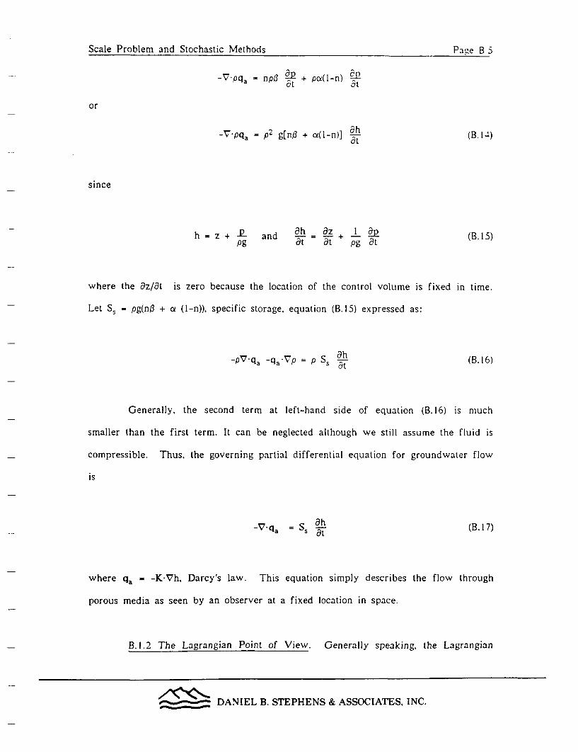
Scale Problem and Stochastic Methods Pag~e B 5
-V7Pqa - npB a + poe(1-n) 0at at
or
-7-pqa = P2 g[n3 + a(l-n)] ah (B. 14)
since
h = z + P and ah = az + I appg at at pg at (B. I5)
where the az/at is zero because the location of the control volume is fixed in time.
Let S, = pg(n/3 + a (I-n)), specific storage, equation (B.l5) expressed as:
-p7.q, -q,.Vp = P Ss aat (B. 16)
Generally, the second term at left-hand side of equation (B.16) is much
smaller than the first term. It can be neglected although we still assume the fluid is
compressible. Thus, the governing partial differential equation for groundwater flow
is
-7-q. = S., ah= sat (B.17)
where qa = -K Vh. Darcy's law. This equation simply describes the flow through
porous media as seen by an observer at a fixed location in space.
B.1.2 The Lagrangian Point of View. Generally speaking, the Lagrangian
/e___ DANIEL B. STEPHENS & ASSOCIATES, INC.
Scale Problem and Stochastic Methods Pi-kFe B 6
approach in fluid mechanics implies that observations are made by followinmz the
fluid flow. Flow in deformable porous media. however, involves the nmovenlent of
both fluid and solids. Since most of our monitoring devices such as observation
wells are installed in the geologic formations, our observations are likely following
the movement of solid grains as the formations undergo deformation. In this section,
we will derive the governing groundwater flow equation from the Lagrangian point
of view (i.e.. by following the mean displacement of the solid grains instead of the
fluid.)
The classical form of Darcy's law applies in effect to the velocity of the
fluid in relation to that of the solid and not in relation to stationary space. From the
Eulerian point of view, the specific discharge. qa, is then
qa = qW + nv, (B. 18)
where q, represents the specific discharge of the fluid in the classical Darcy's law,
n is the porosity, and vs is the solid velocity in the vertical direction since we will
assume the porous medium undergoes vertical deformation only.
Using (B.18), the continuity equation defined in relation to a fixed point in
space, (8.8), becomes
-'vp(qw + nvs) = -Vpqw - apnv5 = (B. 19)az at
where the second term represents the net solid mass flux over the control volume.
Equation (B.19) can be further expanded to
-v pqw - nv, aP - pv an - pn a-v - n aao + p an
______ DANIEL B. STEPHENS & ASSOCIATES, INC.

Scale Problem and Stochastic Methods Place B 7
-pq, = n do + P dn + pn avdt dt a~~z
(B.20)
where dp/dt and dn/dt are the substantial derivatives of p and n, respectively. with
respect to the v1. That is. the rate of changes in fluid density and porosity as seen
by an observer moving at the mean velocity of solid grains.
The substantial derivative of p can be expressed as
dp = p + V Vpdt at
Since the second term on the right-hand side of the equation is small, it can be
neglected. The rate of change in fluid density can be related to compressibility of
the fluid as we did previously.
n ~Dd = n -lP dP = npf dPdt- dp dt- dt
(8.21)
However, the rate of change of porosity deserves some elaboration. Consider solid
volume conservation in a control volume. The continuity equation is
av S - v)at~ = -(V.V~vs (B1.22)
Recognizing that V. - (I-n)VT and VT is constant. equation (B.22) can be rewritten
in the form of
_______ DANIEL B. STEPHENS & ASSOCIATES, INC.

Scale Problem and Stochastic IMethods Pace B SScale Problem and Stochastic N~~~~~~~~ethods Pace B S~~
(I-n) 5 _ na +v n = dnCZ CZS dt
(E3. 3)
Assuming each individual solid grain does not deform. the density of solids should
remain constant. A solid mass balance leads to
am-V ms v5 = at and
ams ams dm5 avsat + VS az dt S z
I d(ms l/p) I dV, I dV, dre adoe X
mS /Ps dt Vs dt Vs dre dt dt dt
(13.24)
(B. 25)
and
Substituting (B.21),(B.23), and (B.25) into (B.20), one obtains
-v -pq= - p(n: + a) d2dt (B. 26)
Note that
h = z + D and dh = dz + I Xpg dt dt pg dt
(B.27)
and the dz/dt is zero because the location of the reference point is stationary as
seen by an observer following the displacement of the solid. Equation (B.27) thus
becomes:
_____ DANIEL B. STEPHENS & ASSOCIATES, INC.
Scale Problem and Stochastic Methods Pave B 9
-PV7qW -qW -'VP = P. g(n3 + a) dh (13.2S)dit
Assuming that pV7qw >>qw Vp and applying Darcy's law to (B.28). one obtain the
governing groundwater flow equation from the Lagrangian point of view:
V (K-Vh) = Ss dh (B.29)dt
where S, - pg(n/3 + a) and is called specific storage. Note the expression of specific
storage is different from the one in equation (B.17) which is derived from the
Eulerian point of view. Theoretically, equation (B.29) is the correct one for field
applications because our observations generally follow the displacement of the grains
as the aquifer deforms.
However, the velocity of the solid is small. Many convenient but misleading
assumptions have been employed for practical purposes. For example, the coefficients
of compressibility of water, g, and porous matrix, a, in the fixed coordinate system
are assumed the same as those in the moving coordinate system. They are, in effect,
different. Moreover, based on the same argument, the dh/dt is replaced by ah/at and
hydraulic conductivity is assumed constant in time even if the porous medium is
deformable. These misleading assumptions lead to the classical governing groundwater
flow equation which is given as:
V (K-Vh) - pg(ng + a) -5-1= Ss ,6ih (B.30)
This equation is theoretically inconsistent since it mixes the expressions for both the
fixed and moving coordinate systems.
DANIEL B. STEPHENS & ASSOCIATES, INC.

Scale Problem and Stochastic Methods Page B10
The inconsistency of the classic groundwater equation mav not, however.
have significant impacts on the analysis of groundwater flow. This results from the
fact that the hydraulic head in the field is indeed observed following the
displacement of the solid grains. The specific storage is often estimated from aquifer
tests and the analysis of the test data does not require the use of the expressions for
S. Furthermore, the error in the estimation of Ss and K from field data may be so
large that misleading assumptions may not play any critical role in the analysis of
groundwater flow.
______ - DANIEL B. STEPHENS & ASSOCIATES, INC.

Scale Problem and Stochastic Methods Page C I
Bibliography on Geostatistical and StochasticMethods Related to Groundwater-Hydrology
Ababou, R. and L.W. Gelhar, Three-dimensional groundwater flow in random media:Direct simulation versus spectral theory. EOS, 68(44), Nov. 3, 1987.
Ahlstrom, S.W., 1975. Modeling the transport of selected rationuclides in subsurfacewater systems using the discrete-parcel-random-walk approach. Trans. Am.Geophys. Union, V56(12), 979
Ahlstrom, S.W. and H.P. Foote. 1976, Transport modeling in the environment usingthe discrete-parcel-walk approach, NTIS Accession No. BNWLSA-5528
Alpay. O.A., 1972, A practical approach to defining reservoir hereogeneity. J. Petrol.Technol., V20(7). 841-848
Anderson. M.P., 1979, Using models to simulate the movement of contaminantsthrough groundwater flow systems. Crit. Rev. in Env. Controls 9(2):97-156
Andersson, J. and A.M. Shapiro, 1983, Stochastic analysis of one-dimensional steadystate unsaturated flow: a comparison of Monte Carlo and perturbationmethods, Water Resour. Res., 19(1), 121 133
Arya, A., T.A. Hewett, R. Larson, and L.W. Lake, 1985. Dispersion and reservoirheterogeneity, Society of Petroleum Engineers, SPE14364, Presented at the60th Annual Technical Conference of the Society of Petroleum Engineers,Las Vegas, Nevada, Sept. 22-25
Bachmat. Y., 1969. Hydrodynamic dispersion in a saturated homogeneous porousmedium at low Peclet numbers and nonhomogeneous solution, Water Resour.Res., V5(1), 139-143
Bachmat, Y., 1972, Spatial macroscopization of processes in heterogeneous systems.Israel J. of Technology, V10(5), 391
Bachmat, Y., 1976. Annual operation of a coastal groundwater basin at a prescribedreliability level. J. Hydrol., V31 (1-2), 97-118
Bachmat, Y. and J. Bear, 1964. The general equations of hydrodynamic dispersion inhomogeneous isotropic porous mediums, J. Geophy. Res. V69(12), 2561-2567
Bakr, A.A., Stochastic analysis of the effect of spatial variations in hydraulicconductivity on groundwater flow, Ph.D. dissertation, New Mexico Instituteof Mining and Technology, Socorro. July 1976
Bakr, A.A., L.W. Gelhar, A.L. Gutjahr, and J.R. MacMillan, 1978, Stochasticanalysis of spatial variability in subsurface flows, 1. Comparison of one- andthree-dimensional flows, Water Resour. Res., V14(2). 263-271
Barrenblat. G.E., I.P. Zheltov, and J.N. Kochina, 1960, Basic Concepts in the theoryof homogeneous liquids in fissured rocks, J. Appl. Math. Mech. USSR, 24(5): 1286-1303
Bastin. G., Stochastic parameter estimation of a steady-state groundwater flow model,
DANIEL B. STEPHENS & ASSOCIATES. INC.

Scale Problem and Stochastic Methods Pace C2
Paper presented at the Congress on Simulation of Systems. Sorrento. Italy,September 24-28, 1979
Batchelor. G.K., 1974, Transport properties of twvo-phase materials with randomstructure, Annu. Rev. Fluid Mech., V6. 227-257
Bathala, C.T.. A.R. Rao. and J.A. Spooner, 1977. Application of linear systemsanalysis to ground water evaluation studies. Tech. Rep. No. 91, WaterResour. Res. Center. Purdue Univ., West Lafayette. Indiana. 128
Bathala, C.T.. A.R. Rao, and J.A. Spooner, 1977. Stochastic- models for groundwaterlevels using causal relationships. Abstract in Hydraulics in the Coastal Zone,ASCE. New York, p. 211
Bathala. C.T., J.A. Spooner, and A.R. Rao, 1976, Regional aquifer evaluation studieswith stochastic inputs, Tech. Rep. No. 72, Purdue Univ.. Water Resour. Res.Center. West Lafayette, Indiana
Bear. J., 1961. On the tensor form of dispersion in porous media. J. Geophys. Res.,V66(4), 1185-1197
Bear, J., 1961. Some experiments in dispersion, J. Geophys. Res., V66(8), 2455-2468
Bear. J., 1972. Dynamics of fluids in porous media, 764 p., American Elsevier, NewYork
Bear, J., 1979, Hydraulics of Groundwater, 569 pp., McGraw-Hill, New York
Bear. J. and Y. Bachmat, 1967, A generalized thoery on hydrodynamic dispersion inporous media. Int. Assn Sci. Hydrol Symp., Haifa. Publ. 72, 7-16, March1967
Bellomo, N. and R. Monaco, 1979, Mathematical models for the time-evolution ofstochastic systems in two-phase flow, Appl. Math Modeling, V3(1), 41-44Bennion. D.W., and J.C. Griffiths, 1966, A stochastic model for predictingvariations in reservoir rock properties, Trans. AIME, No. 237, Part 2, 9-16
Bennion, D.W., and J.C. Griffiths, A stochastic model for predicting variations inreservoir rock properties, Trans. AIME. No. 237, Part 2, 9-16. 1966.
Beran, M.J., 1957, Dispersion of soluble matter in flow through granular media, J.Chem. Phys., V27, 270-274
Beran. M.J., 1968, Statistical continuum theories. Interscience, New York
Betson, R.P., J.M. Boggs, S.C. Young, L.W. Gelhar, 1985, Design of a fieldexperiment to investigate groundwater saturated zone transport processes,Interim rpt, RP2485-05. 104pp., Elecr. Power, Res. Inst., Palo Alto, CA
Bhattacharya. R.N.. V.K. Gupta, and G. Sposito. 1976. Markovian stochastic basis fortranport of water through unsaturated soil, Soil Sci. Soc. Am. J., V40(3),465-467
Bhattacharya, R.N., V.K. Gupta, and G. Sposito, 1976, On the stochastic foundations
DANIEL B. STEPHENS & ASSOCIATES, INC.
Scale Problem and Stochastic Methods Par~e C 3)
of the theory of water flow through unsaturated soil. Water Resour. Rcs..V12(3), 503-512
Bhattacharya. R.N., V.K. Gupta, and G. Sposito. 1976. Physical interpretation of soil-water diffusivity in terms of theory of Nlarkov-processes, Soil Sci.. V121(3)313-314
Bhattacharya. R.N., V.K. Gupta. 1979. Statistical-theory of solute transport in porousmedia, SIAM J. on Applied Math., V37(3). 485-498
Bibby, R. and D.K. Sunada. 1971. Statistcal error analysis of a numerical model ofconfined groundwater flow, in Stochastic Hydraulics: Proc. First Int. Symp.on Stochastic Hydraul., C.L. Chiu, ed., 591-612. 1971, School of Engineering,University of Pittsburgh. Pittsburgh, Pennsylvania
Black. T.C. and D.L. Freyberg, 1987. Stochastic modeling of vertically averagedconcentration uncertainity in a perfectly stratified aquifer, Water Resour.Res. 23(6): 997-1004
Bogardi, 1. and L. Duckstein. Design of a foundation subject of random groundwaterlevels. in Hydraulic Engineering for Improved Water Mangement. Proc. 17thCongress of Int. Assn for Hydraul. Res.. 15-19 August 1977, Vol 6, 383-389
Bogardi, I., L. Duckstein. A. Schmieder, and F. Szidarovszky, 1980, Stochasticforecasting of minewater inrushes, Adv. in Water Resour., V3(1). 3-8
Bonano, E.J. and R.M. Cranwell. 1988, Treatment of uncertainties in the performanceassessment of geologic high-level radioactive waste repositories, Math. Geol..20(5), 543-565
Bonano, E.J., L.R. Shipers. A.L. Gutjahr, 1987. Stochastic analysis of contaminanttransport in porous media: analysis of a two-member ratio nuclide chain,Water Resour. Res. 23(6): 1063-1078
Boreli, M., M. Radojkovic, and S. Jovic. Some fundamental problems of undergroundwater pollution, in Hydraulic Engineering for Improved Water Management,Proc. 17th Congress of Int. Assn for Hydraul. Res., 15-19 August 1977, Vol6, 714-717
Bouwer, H., 1969, Planning and interpreting soil permeability measurements. J. IrrDrain Div., ASCE. V95(3), 391-402
Bras, R.L. and I. Rodriguez-Iturbe. 1985, Random functions and hydrology. Addison-Wesley publishing company, 559pp.
Bresler, E., H. Bielorai, and A. Laufer, 1979, Field test of solution flow models in aherogeneous irrigated cropped soil. Water Resour. Res., V15(3), 645-652
Bresler, E. and G. Dagan. 1979. Solute dispersion in unsaturated heterogeneous soil atfield scale, 2. Applications, Soil Sci. Soc. Am. J. 43:467-472
Broadbent, S.R. and J.M. Hammersley, 1957, Percolation processes, crystals andmazes, Proc. Cambridge Phil. Soc., V53. 629-641
________ DANIEL B. STEPHENS & ASSOCIATES, INC.

Scale Problem and Stochastic Methods Pave C 4
Brown, M.C.. 1973. Mass balance and spectral analysis applied to karst hydraulicnetworks. Water Resources Res., V9(3), 749-752
Bulnes, A.C.. 1946. An application of statistical methods to core analysis data ofdolomitic limestone, Trans. AlIME, 165. 223-240
Burrough, P.A., 1983a, Multiscale sources of spatial variation in soil, 1: Theapplication of fractal concepts to nested levels of soil variation, J. SoilScience, 34. 577-597
Burrough, P.A., 1983b, Multiscale sources of spatial variation in soil, 11: A non-Brownian fractal model and its application in soil survey, J. Soil Science, 34,599-620
Butler. Jr.. J.J.. Pumping tests in nonuniform aquifers: a deterministic/stochasticanalysis, Ph.D. dissertation, Stanford University, Stanford. CA.. 220 pp.,December 1986
Butler, S.S. and D.L. Gundlach. 1972, Discharge and travel time for nonuniformgroundwater conduits, Trans. Am. Geophys. Union. V53(11), 980 Buyevich,Y.A.. A.l. Lenov. and V.M. Safrai. 1969, Variations in filtration velocitydue to random large scale fluctuations in porosity, J. Fluid Mech., V37(2),371-381
Byers, E. and D.B. Stephens, 1983, Statistical and stochastic analysis of hydraulicconductivity and particle size in a fluivial sand, Soil Sci Soc Am J..47: 1072-1081
Carnahan. C.L., 1976, Nonequilibrium thermodynamics of groundwater flow systems--symmetry properties of phenomenological coefficients and conservations ofhydrodynamic dispersion, J. Hydrol. V31(I-2), 125-150
Carrera. J. and S.P. Neuman, 1986, Estimation of aquifer parameters under transientand steady state conditions, 1. Maximum likelihood method incorporatingprior information, Water Resour. Res. 22(2):199-210
Carrera. J. and S.P. Neuman, 1986, Estimation of aquifer parameters under transientand steady state conditions, 2. Uniqueness, stability, and solution algorithms,Water Resour. Res. 22(2):211-227 %
Carrera, J. and S.P. Neuman, 1986. Estimation of aquifer parameters under transientand steady state conditions, 3. Application to synthetic and field data, WaterResour. Res. 22(2):228-242
Cavazza. S., 1964, Relationship between rainfall intensity and groundwater movementin subfluvial aquifers, in General Assembly of Berkeley, August 1963, Int.Assn Sci. Hydrol. Publ. No. 64, 390-401
Chander, S., P.N. Kapoor, and S.K. Goyal. 1981, Aquifer parameter estimation usingKalman filters. J. Irrigation and Drainage Div., ASCE, V107(IRI), 25-33
Charbeneau, R.J.. and H-D. Yeh. 1979, Conditional simulation of groundwater flowfields with emphasis on regional dispersion, Trans. Am. Geophys. Union.V60(46). 821
________ DANIEL B. STEPHENS & ASSOCIATES, INC.

Scale Problem and Stochastic Methods Pave C SScale Problem and Stochastic Methods Pace CS~~~~~~~~
Chaudhari, N.M. and A.E. Scheidegger, 1965. Statistical mechanics of certainhyrodynamic dispersion phenomena. Can. J. Phys.. \V43(10). 1776-1794
Chirlin, G.R. and G. Dagan, 1980. Theoretical head variograms for steady flow instatiscally homogeneous aquifers, Water Resour. Res.. V16(6), 1001-1015
Chirlin, G.R. and E.F. Wood, 1979, Some theoretical and practical problems invariogram estimation and application. Trans Am. Geophys. Union. V60(46).820 Chow, V.T. and S.J. Kareliotis. 1970, Analysis of stochastic hydrologicalsystems, Water Resour. Res., V6(6), 1569-1582
Chu, S.T., 1977, Water table response to a sequence of recharges. Water Resour.Res.. V13(4). 739-742
Clapp, R.B., G.M. Hornberger, and B.J. Cosby, 1981, Estimating spatial variability insoil moisture with a dynamic cmodel and Monte-Carlo simulation, Trans.Am. Geophys. Union, V62(17), 287
Clifton, P.M., and S.P. Neuman. 1982. Effects of kriging and inverse modeling onconditional simulation of the Avra Valley aquifer in southern Arizona,Water Resour. Res., 18, 1215-1234
Clifton, P.M., B. Sagar. and R.G. Baca, 1985, Stochastic groundwater traveltimemodeling using a Monte Carlo technique, In International Association ofHydrogeologists Memoires: Hydrogeology of Rocks of Low Permeability.Tucson, Arizona, 17(1), 319-329
Codell, R., Draft generic position on groundwater travel time, Div. of Waste Manag..Office of Nuclear Material Safety and Safeguards, U.S. Nuclear RegulatoryCommisssion. June 30, 1986
Cole, C.R. and H.P. Foote. Use of a multigrid technique to study effects of limitedsampling of heterogeneity on transport prediction, Presented at the NationalWater Well Association Conference, Solving Ground Water Problems withModels, Denver, Colorado, February 10-12, 1987
Cooley, R.L., 1979, A method of estimating parameters and assessing reliability formodels of steady-state groundwater flow, 2. Application of statistical analysis,Water Resour. Res., V15(3), 603-617
Cooley, R.L., J.W. Fordham, and J.A. Westphal, 1973, Some applications of statisticalmethods to groundwater flow system analysis, Tech. Rept. Series H-W,Hydrology and Water Resources Pub. No. 14, 53 p.. Desert ResearchInstitute. University of Nevada, Reno, Nevada
Csanady, G.T., 1973, Turbulent diffusion in the environment, D. Reidel PublishingCo., 248 pp.
Cushman, J.H., 1983, Volume averaging, probabilistic averaging, and ergodicity, Adv.Water Resour. 6:182-184
Cushman, J.H.. 1984. On unifying the concepts of scale, instrumentation, andstochastics in the development of multiphase transport theory. Water Resour.Res. 20( ): 1668-1676
_______ DANIEL B. STEPHENS & ASSOCIATES, INC.

Scale Problem and Stochastic Methods Paie C6
Cushman. J.H., 1986. On measurement, scale. and scaling. Water Resour. Res.22:129-134
Cushman, J.H., 1987, More on stochastic models, Water Resour. Res. 23(4):750-752
Dagan, G., 1967, Hydrodynamic dispersion in a nonhomogeneous porous column, J.Geophys. Res., V72(4), 4075-4080
Dagan. G., 1976, Comment on "A stochastic-cnceptual analysis of one-dimensionalgroundwater flow in nonuniform homogeneous media" by R.A. Freeze,Water Resour. Res., V12(3), p 567
Dagan, G.. 1979, Generalization of Darcy law for nonuniform flows. Water Resour.Res., V15(1), 1-7
Dagan, G., 1979, Models of groundwater flow in statistically homogeneous porousformations. Water Resour. Res., V15(l), 47-63
Dagan, G., 1980, Correction, Water Resour. Res., V16(l), 255, to: Miodels ofgroundwater flow in statistically homogenous porous formations. WaterResour. Res.. 15(1), 1979
Dagan. G., 1981, Analysis of flow through heterogeneous random aquifers by themethod of embedding matrix, 1. Steady flow, Water Resour Res., V 17(l),107-121
Dagan, G.. Solute transport in heterogeneous porous formation, J. Fluid Mech.. 145.151-177, 1984.
Dagan, G., 1986, Statistical theory of groundwater flow: pore - to laboratory -,
laboratory - to formation, and formation - to regional scale, Water Resour.Res. 22(9): 1205-1345
Dagan, G., 1987, Theory of solute transport by groundwater, Ann. Rev. Fluid Mech.,19, 183-215
Dagan, G. and E. Bresler, 1979, Solute-dispersion in unsaturated heterogeheous soilat field scale, 1. theory, Soil Sci. Soc. Am. J., V43(3), 461-467
Davidson, M.R. and B.L. Dickson, 1986, A porous flow model for steady statetransport of radium in groundwater, Water Resour. Res. 22(l):34-44
Davis, J.C., 1973, Statistics and Data Analysis in Geology, 550 pp.. John Wiley andSons, Inc., New York
Debouche. Ch., S. Gaspar, and L. Sine, 1974, Diffusivite de leau dans un milieu nonsature heterogene, J. Hydrol. V22(1-2), 35-51
DeJosselin de Jong, G., 1958, Longitudinal and transverse diffusion in granulardeposits, Trans. Am. Geophys. Union, V39(1), 67-74
DeJosselin de Jong, G., 1972, The tensor characteristics of the dispersion coefficientin anisotropic porous media, in Fundamentals of Transport Phenomena inPorous Media, Elsevier, Amsterdam, 1972, 259-267
________ DANIEL B. STEPHENS & ASSOCIATES, INC.
Scale Problem and Stochastic Methods Pagze C 7Scale Problem and Stochastic Methods Pace C 7~~~~~~~~~~~~~~~~~~~~~~~~~~~~~~~~
DeJosselin de Jong, G. and M.J. Bossen, 1961, Discussion of paper hy Jacob Bear"On the tensor form of dispersion in porous media". J. Geophys. Res.,V66(10), 3623-3624
Delhomme, J.P., 1978, Kriging in the hydrosciences, Adv. in Water Resour.. Vi(5).251-266
Delhomme, J.P., 1979, Kriging under boundary conditions, Trans. Am. Geophy.,Union. V60(46), 820
Delhomme, J.P., 1979, Spatial variability and uncertainty in groundwater flowparameters: A geostatistical approach, Water Resour. Res., V15(2), 269-280
De Marsily, G., 1984. Spatial variability of properties in porous media: a stochasticapproach, in Fundamentals of Transport in Porous Media, J. Bear, Y.Corapcioglu (eds.), Nijhoff, Dordrecht, pp. 721-769
De Marsily, G., G. Lauedan, M. Boucher, G. Fasanino, 1984, Interpretation ofintereference tests in a well field using geostatistical techniques to fit thepermeability distribution in a reservoir model. in Geostatistics for NaturalResources Characterization, Proc. NATO-ASI, Berly et al. (eds.) Part 2,Reidel Pub. Co. Dordrecht, The Netherlands
De Marsily. G., 1985, Flow and transport in fractured rocks: connectivity and scaleeffect, Mem. Int. Assoc. Hydrogeol. 17:267-277
De Marsily, G., 1986, Quantitative Hydrogeology: Groundwater Hydrogeology forEngineers, 440 pp.. Academic Press, Inc., Orlando, Florida
Dendrou, B.A., E.N. Houstis, and S.A. Dendrou, 1979, Site selection using a kriging-FEM scheme. Trans. Am. Geophys. Union, V60(46), 821
Desbarats, A.J., 1987, Numerical estimation of effective permeability in sand-shaleformations, Water Resour. Res. 23(2):273-286 Dettinger, M.D. and J.L.Wilson, 1981, First-order analysis of uncertainty in numerical models ofgroundwater flow, 1. Mathematical description, Water Resour. Res.17:149-161
Devary, J.L. and P.G. Doctor, 1982, Pore velocity estimation uncertainties, WaterResour. Res. 18(4):1157-1164
Dievlin, A., G. Matheson, G. de Marsily, 1981, Growth of the dispersion coefficientwith the mean travelled distance in porous media, Sci. Total Env. 21:319-328
Domenico, P.A. and G.A. Robbins, 1984, A dispersion scale effect in modelcalibrations and field tracer experiments, J. Hydrol. 70:132-
Dooge, J.C.I., Scale problems in hydrology. Kisiel Memorial Lecture at Department ofHydrology and Water Resources, University of Arizona, Tucson, Arizona,February 19, 1986
Dracup, J.A.. O.E. Drummond. and P.R. Westlake, 1978, Kalman filtering of waterwell fluctuations, in Applications of Kalman Filter to Hydrology, Hydraulics,and Water Resouces, C.L. Chiu, ed., Stochastic Hydraulics Program,
________ DANIEL B. STEPHENS & ASSOCIATES, INC.
Scale Problem and Stochastic Methods ['age C 8Scale Problem and Stochastic Methods Pace C8
University of Pittsburg, Pennsylvania. 693-275
Driscoll, F.G.. 1986. Groundwater and Wells, 10S9 pp.. Johnson Division. St. Paull,Minnesota
Duerbaumr. H.J. and K. Trippler, 1972, Comparison of statistical and deterministricapproaches in the determinationof hydrological parameters of aquifers, inProc. Int. Symp. on Uncertainties in Hydrologic and Water ResourceSystems, Vol. 3, 3.3-1-3.3-20. Department of Hydrol. and Water Resour.,University of Arizona, Tucson
Duffy, C.J. and L.W. Gelhar, 1986, A frequency domain analysis of groundwaterquality fluctuations: interpretations of field data, Water Resour. Res.22(7):1 115-1128
Duffy, C.J. and J. Harrison, 1987. The statistical structure and filter characteristics oftritium fluctuations in fractured basalt, Water Resour. Res. 23(5):894-902
Dullien, F.A.L.. 1979, orous media-fluid transport and pore structure, 396 p.,Academic Press, New York, NY
Elgizawi. M.G., 1974. Use of cross-correlation techniques for determining therelationship between groundwater levels and sources in the Nile delta area,in Mathematical Models in Hydrology, Proc. of the Warsaw Symp., July1971, Int. Assn Hydrol. Sci. Publ. No. 100, 319-325
Elsworth. D., A boundary element-finite element procedure for porous and fracturedmedia flow, Water Resour. Res., 23(4), 551-560, 1987
Eriksson. G., 1970, Cross-spectrum analysis of groundwater levels in an esker, Nord.Hydrol., VI(4). 245-259
Eriksson, G., 1970, Groundwater time-series: An exercise in stochastic hydrology,Nord. Hydrol. VI(3), 181-205
Fara, H.D., and A.E. Scheidegger, 1961, Statistical geometry of porous media. J.Geophys. Res., V66(10), 3279-3284
Ferrandon, J., 1948, Lew lois de l'ecoulement de filtration, Le Genie Civil, V 125,24-28
Ferraund. L.A. P.C.D. Milly, G.F. Pinder, 1986, Dual-gamma attenuation for thedetermination of porous medium saturation with respect to three fluids.Water Resour. Res. 22(12):1657-1663
Fischer, H.B.,E.J. List. R.C.Y. Koh, J. Imberger, N.H. Brooks. 1979, Mixing in inlandand coastal waters, Academic press, 483 pp.
Flores, W., E.Z., A.L. Gutjarh. and L.W. Gelhar, 1978. A stochastic model of theoperation of a stream-aquifer system, Water Resour. Res., V14(l), 30-38
Fogg, G.E., 1986, Groundwater flow and sand body interconnectedness in a thickmultiple-aquifer system, Water Resour. Res. 22(5):679-694
DANIEL B. STEPHENS & ASSOCIATES, INC.

Scale Problem and Stochastic Methods Page C 9Scale Problem and Stochastic Methods Pa~~~~~~~~~~~~~~~.'e C9~
Freeze, R.A., 1971, Three-dimensional, transient, saturated-unsaturated flow in agoundwater basin, Water Resour. Res.. 7(2), 347-366
Freeze, R.A.. 1975. A stochastic-conceptual analysis of one- dimentional groundwaterflow innonuniform homogeneous media. Water Resourc. Res., VI 1(5), 725-741
Freeze., R.A., L.W. Gelhar,and T. Maddock, 1978. Geostatistical concepts andstochastic methods in hydrogeology, Geology. V6(5), 297-298
Freyberg, D.L.. 1986, A natural gradient experiment of solute transport in a sandaquifer 2. Spatial moments and the advection and dispersion of nonreactivetracers. Water Resour. Res.. 22, 2031-2046
Fried, J.J. and M.A. Combarnous, 1971, Dispersionin porous media, in Advances inHydroscience, V 7. 169-282
Frisch, H.L., and J.M. Hammersley, 1963, Percolation processes and related topics, J.Soc. Ind. Appl. Math., V1l(4), 894-918
Gambolati, G., 1979, Kriging in the environmental applications: results andshortcomings. Trans. Am. Geophys, Union, V60(45), 821
Gambolati. G. and G. Volpi, 1979, A conceptual deterministic analysis of the Krigingtechnique inhydrology, Water Resour, Res., V15(3), 625-629
Gambolati, G. and G. Volpi, 1979, Groundwater countour mapping in Venice bystochastic interpolators, 1. Theory, Water Resour, Res., V15(2). 281-290
Ganoulis. J. and C. Thirriot, 1973, Sur un modele probabiliste de l'equilibre capillaireen milieu poreux C. R. Acad. Sc. Paris, T. 276, Ser. A, 1573-76
Ganoulis. J. and C. Thirriot, 1977, Stochastic study of the entrance of a non-wettingfluid in a pourous medium, under the influence of capillarity in "Hydraulicprobems solved by stochastic methods", Proc. 2e Int. IAHR Symp. onStochastic Hydraulics, Lund, Sweden, Aug. 2-4, 1976,Water Res. Publ., pp22.1-22.18, Fort Collins, Colorado 80522
Gannon, John M., and T.-C.J. Yeh, Numerical analysis of the effects ofheterogeneities on dispersion, in prep 1988.
Garabedian. S.P., Large-scale dispersive transport in aquifers: field experiments andreactive transport theory, PhD. dissertation, Massachusetts Institute ofTechnology, Cambridge, Massachusetts, July 1987
Gavalas, G.T.. P.C. Shah, and J.H. Seinfeld, 1976. Reservoir history matching byBayesian estimation, Soc. Petrol. Eng. J., V16(6), 337-350
Gelhar. L.W.. 1974, Stochastic analysis of phreatic aquifers, Water Resour. Res.,V 10(3), 539-545
Gelhar, L.W.. 1976. Effects of hydraulic conductivity variations on groundwaterflows, in Hydraulic Problems Solved by Stochastic Methods, Proc. SecondInt. IAHR Symp on Stochas- tic Hydraulics, Lund, Sweden, 409, 429.WaterResourc. Publications, Fort Collins. CO
_______ DANIEL B. STEPHENS & ASSOCIATES, INC.

Scale Problem and Stochastic Methods pagge CoScale Problem and Stochastic Methods Page CO~~~~~~~~~~~~~~~~~~~~~~~~~~~~~~~~~~~~~~~~~~~~~~~~~~~~~~~~~~~~~~~~~~~~~~~~~~~~~
Gelhar, L.W., A.A. Bakr. A.L. Gutjahr, and J.R. McMillan, Comments on stochasticconceptual analysis of one-dimensional groundwater flow in a non-unil romhomogeneous medium by Freeze, R.A.. Water Resour. Res. 13(2), 477-4S0.1977.
Gelhar, L.W.. A.L. Gutjahr, and R.L. Naff, Stochastic analysis of macrodispersionin a stratified aquifer, Water Resour. Res., 15, 1387-1397. 1979.
Gelhar, L.W., 1984, Stochastic analysis of flow in heterogeneous porous media inFundamentals of Transport Pheonmena in Porous Media. J. Bear and M.Y.Corapcioglau (eds.), Martinus Nijhoff Publishers, Dordrecht, The Netherlands
Gelhar, L.W.. 1986, Stochastic subsurface hydrology: from theory to applications.Water Resour. Res. 22(9):1355-1455
Gelhar. L.W.. 1988, Response to O.E. Meinzer Award. GSA Bulletin. July. p. 948.
Gelhar, L.W. and C.L. Axness. 1983, Three-dimensional stochastic analysis ofmacrodispersion in aquifers, Water Resour. Res.. 19(1). 161-180
Gelhar. L.W., A.A. Bakr, A.L. Gutjahr, and J.R. MacMillan, 1977. Comments on "Astochastic-conceptual analysis of one- dimensional groundwater flow innonuniform homogeneous media" by R.A. Freeze, Water Resourc. Res..V13(2), 477-479
Gelhar, L.W. and M.S. Collins, 1971, General analysis of longitudinal dispersion innonuniform flow, Water Resour. Res., V7(6), 1511-1521
Gelhar, L.W., G.W. Gross, and C.J. Duffy, 1979, Stochastic methods of analyzing,groundwater recharge, in the Hydrology of Areas of Low Precipitation, Proc.of Canberra Symp., Int. Assn Hydrol Sci Publ No. 128, 313-321
Gelhar, L.W., A.L. Gutjahr, and R.L. Naff. 1979, Stochastic analysis ofmacrodispersion in a stratified aquifer, Water Resour. Res., VI15(6),1387-1397
Gelhar, L.W., P.Y. Ko, H.H. Kwai. and J.L. Wilson, 1974, Stochastic modelling ofgroundwater systems, 313 p.. Rep. 189, R.M. Parsons Lab for Water Resour.and Hydrodynamics. Massachusetts Institute of Technology, Cambridge,Massachusetts
Gelhar, L.W., J.L. Wilson, and A.L. Gutjahr, 1979. Comments on "Simulation ofgroundwater flow and mass transport under uncertainty" by D.H. Tang andG.F. Pinder, Adv. in Water Resourc., 2(2), 101
Gillham, R.W., E.A. Sudicky, J.A. Cherry, E.O. Frind, 1984, An advection-diffusionconcept for solute transport in heterogeneous unconsolidated geologicaldeposits, Water Resour. Res. 20(3):369-378
Golden, J.M., 1980, Percolation theory and models of unsaturated porous media,Water Resour. Res., V16(1), 201-109
Greenkorn, R.A. and D.P. Kessler, 1969, Dispersion in heterogeneous nonuniformanisotropic porous media, Ind. Eng. Chem., V61(9), 14-32
________ DANIEL B. STEPHENS & ASSOCIATES, INC.

Scale Problem and Stochastic Methods P.ige ClIScale Problem and Stochastic Methods Pace 0 I
Gupta. V.K. and R.N. Bhattacharya, 1986. Solute dispersion in multidimensionalperiodic saturated media, Water Resour. Res. 22(2):156-164
Gutjahr. A.L.. Kriging in stochastic hydrology: Assessing the worth of data, paperpresented at the Chapman Conference on Spatial Variability in HydrologicModeling. AGU. Fort Collins, Colorado. July 1981
Gutjahr, A.L. and L.W. Gelhar. 1981, Stochastic models of subsurface flow: Infiniteversus finite domains and stationarity, Water Resour. Res., V17(2), 337-350
Gutjahr, A.L., E.J. Bonano. R.M. Cranwell, 1985. Treatment of parameteruncertainties in modeling contaminant transport in geologic media: stochasticmodels versus determination models with statistical parameter sampling, inProc. Int's Assoc. Hydraulic Research Symp. in the Stochastic Approach toSubsurface Flow, G. de Marsily (ed.), Montvillargenne, France, June 3-6,1985, pp. 332-350
Gutjahr, A.L., L.W. Gelhar, A.A. Bakr. and J.R. MacMillan, 1978, Stochasticanalysis of spatial variability in subsurface flows, 2. Evaluation andapplication. Water Resourc. Res., V14(5), 953-960
Gutjahr. A.L.. D. McKay, and J.L. Wilson, Fast Fourier transform methods forrandom field generation, EOS, 68(44), Nov. 3. 1987.
Guven, O., F.J. Molz, J.G. Melville, 1984, An analysis of dispersion in a stratifedaquifer, Water Resour. Res. 20: 1337-1354
Guven, O., F.J. Molz, J.G. Melville, 1986, Comment on "an advection-diffusionconcept for solute transport in heterogeneous unconsolidated geologicaldeposit" by Gillham et al., Water Resour. Res. 22(l):89-91
Guven. 0. and F.J. Molz, 1986, Deterministic and stochastic analysis of dispersion inan unbounded stratified porous medium, Water Resour. Res. 22(11):1565-1574
Haldorsen, H.H. and L.W. Lake, 1982, A new approach to shale management in fieldscale simulation models, Paper presented at the 57th Annual TechnicalConference, Soc. Pet. Eng.. New Orleans, Sept. 26-29
Haring, R.E. and R.A. Greenkorn, 1970, A statistical model of a porous mediumwith nonuniform pores, AlChE J., V16(3), 447-483
Harleman, D.R.F. and R.R. Rumer, 1963, Longitudinal and lateral dispersion in anisotropic porous medium, F. Fluid Mech.. V16(3), 385-394
Heller. J.P., 1972, Observations of mixing and diffusion in porous media, Proc.Second Int Symp on Fund of Trans Phen in Porpous Media, Int. Assn'Hydraulic Res., 1-26, University of Guelph, Guelph, Ontario, Canada
Hewett, T.A.. Fractal distributions of reservoir heterogeneity and their influence onfluid transport, Society of Petroleum Engineers, SPE15386. Presented at the61st Annual Technical Conference of the Society of Petroleum Engineers,New Orlans, Louisiana. October 5-8, 1986
Hoeksema, R.J. and P.K. Kitanidis. 1984, An application of the geostatistical approach
DANIEL B. STEPHENS & ASSOCIATES, INC.
Scale Problem and Stochastic Methods P~age an2
to the inverse problem in two- dimensional groundwater modeling, \WaterResour. Res. 19(3):677-690
Hoeksema. R.J. and P.K. Kitanidis. 1985. Analysis of the spatial structure ofproperties of selected aquifers, Water Resour. Res, 21. 563-572
Horton. R., M.C. Thompson, J.F. McBride, 1987, Method of estimating the travel timeof noninteracting solutes through compacted soil material, Soil Sci. Soc. Am.J. 51(l):48-53
Huang, C. and D.D. Evans. 1985, A 3-dimensional computer model to simulate fluidflow and contaminant transport through a rock fracture system, NUREG/CR-4042, U.S. Nuclear Regulatory Commission, 108 pp.
Hubbert, M.K.. 1940, The theory of groundwater motion. J. of Geol., 48, 785-944
Huyakorn, P.S.. B.H. Lester. and C.R. Faust. 1983a, Finite element techniques ofmodeling groundwater flow in fractured aquifers, Water Resour. Res., 19(4),1019-1035
Huyakorn, P.S., B.H. Lester, and J.W. Mercer, 1983b, An efficient finite elementtechnique for modeling transport in fractured porous media, 1, Single SpeciesTransport, Water Resour. Res., 19(3):841-854
Huyakorn, P.S.. B.H. Lester and J.W. Mercer, 1983c, An efficent finite elementtechnique for modeling transport in fractured porous media, 2, Nuclide decaychain transport. Water Resour. Res., 19(3), 841-854
Ilyin, N.I., and others, 1971, tsenka tochnosti opredeleniya vodopronitsayemostigornykh porod, Moscow, Nedra
Iwasa, Y. and H. Takeuchi. 1971, Dispersive characteristics of flows through porousmedia, in Stochastic Hydraulics, C.L. Chiu, ed., School of Engineering.University of Pittsburg, 613-631
Jackson, R.E., 1973, Evapotranspiration of groundwater, Scientific Series No. 17,Department of the Environment, Inland Waters Directorate, Ottawa, Canada,40p.
Jackson, R.E., 1974, Time-series analysis of groundwater hydrographs from surficialdeposits on Canadian shield, Can. J. Earth Sci., VIl(l), 177-188.
Jackson, R.E., J.A. Gilliland and K. Adamowski, 1973, Time series analysis of thehydrologic regimen of a groundwater recharge area, Water Resour. Res..V9(5), 1411-1419
Javandel, I.. and P.A.. 1969, Witherspoon, A method of analyzing transient fluid flowin multilayered aquifers, Water Resour. Res.. 5(4), 1969
Jenkins, G.M. and D.G. Watts, 1968, Spectral Analysis and its Applications, 525 pp..Holden-Day, Inc., San Francisco
Jensen, J.L., D.V. Hinkley, L.W. Lake. 1987, A statistical study of reservoirpermeability: distributions. correlations and averages, Soc. Petr. Eng..
________ DANIEL B. STEPHENS & ASSOCIATES, INC.
Scale Problem and Stochastic Methods Pce a 3Scale Problem and Stochastic Methods Pace 03
Formation Evaluation. December, pp. 461-468. Journel. A.G.. and CH.iJ.Huijbregts, 1978. Mining Geostatistics, 600 pp.. Academic Press, London
Journel. A.G.. and CH.J. Huijbregts, 600 pp., Mining Geostatistics. Academic Press.London, 1978.
Julian, P.R., 1967, Variance spectrum analysis, Water Resourc. Res.. V3(3), 831-845
Kasansky. A.B.. 1974. A statistical filtration model for the inseepage of melt waterinto frozen ground, in Mathematical Models in Hydrology. Proc. of theWarsaw Symp.. July 1971, Int. Assn Hydrol. Sci. Publ. No. 100. 241-245.Discussion by S. Dyck, Publ No. 102, 1175-1176
Kazemi, H., M.S. Seth. and G.W. Thomas, 1969, The interpretation of interferencetests in naturally fractured reservoirs with uniform fracture distribution. Soc.Pet. Eng. J., Dec.. 463-472
Kilbury, R.K., T.C. Rasmussen. D.V. Evans, A.W. Warrick, 1986, Water and airintake of surface exposed rock fractures in situ, Water Resour. Res.22(10): 1431-1443
Kipp. K.C.. K.G. Stollenwerk, D.B. Grove, 1986, Groundwater transport of strontium90 in a glacial outwash environment, Water Resour. Res. 22(4):519-530
Kiremidjian. A.S. and P. Kruger, 1979, A stochastic model of radionuclide migrationfrom natural and engineered repositories, in Scientific Basis for NuclearWaste Management, V 2, 779-785
Kitanidis, P.K.. 1986, Comment on "Stochastic modeling of groundwater flow byunconditional and conditional probabilities: the inverse problem" by G.Dagan, Water Resour. Res. 22(6):984-986
Kitanidis, P.K., 1986, Parameter uncertainty in estimation of spatial functions: Boysiananalysis, Water Resour. Res. 22(4):499-507
Kitanidis, P.K.. and E.G. Vomvoris, 1983. A geostatistical approach to the inverseproblem in groundwater modeliling (steady-state) and one-dimensionalsimulations, Water Resour. Res., 19(3), 677-690
Koval, E.J., 1963. A method for predicting the performance of unstable miscibledisplacement in heterogeneous media. Soc. Petrol Eng. J. V392), 145-154
Kriz, H., 1972. Statistical processing of long-term observations of groundwaters, J.Hydrol.. V16(l), 17-37
Labadie. J.W. and D.R. Hampton, 1979, Estimation of hydrogeologic parameters foroptimal groundwater basin development, in Mathematical Programming withData Perturbations. A.V. Fiacco, ed., Lecture Notest in Pure and Appliedmathematics, Marcel Dekker, Inc., New York sched. pub. date. 1981
Larson, R.G.. L.E. Scriven, and H.T. Davis, 1981. Percolation theory of two phaseflow inporous media, Chem. Eng. Sci., V36, 57-73
Lau, L.K., W.J. Kaufman, and D.K. Todd, 1959, Dispersion of a water tracer in
_______ DANIEL B. STEPHENS & ASSOCIATES, INC.

Scale Problem and Stochastic Methods Pa ve (14
radial laminar flow through porous media. Inst. Eng. Research Rept 93-5.University of California, Berkeley, 78 p.
Law, A.G., 1974. Stochastic analysis of groundwater level time series in the westernUnited States, Hydrology Paper No. 68, Colorado State University. FortCollins, CO
Law, J., 1944, A statistical approach to the interstitial heterogeneity of sandreservoirs. Trans AIME, v. 155, 202-222
Liao. K.H. and A.E. Scheidegger, 1968. A computer model for some branching-typephenomena in hydrology, Bull. Int. Assn. Sci. Hydrol., V13(l). 5-13
Liao, K.H. and A.E. Scheidegger, 1969, Branching-type models of flow through porousmedia, Bull Int Assn Sci Hydrol, V14(4). 137-145
Liao, K.H. and A.E. Scheidegger, 1970, Statistical models of flow through porousmedia. Pure and Appl. Geophys., V83(6), 74-81
Lippmann. M.J., 1974, Two-dimensional stochastic model of a heterogeneous geologicsystem, Ph.D. thesis, 135 p., University of California, Berkelye. UniversityMicrofilms order no 75-5810
Lippmann. M.J., and P.A. Witherspoon, 1974, Stochastic model to simulate crosssections of layered heterogeneous groundwater systems, Trans. Am. Geophys.Union. V55(12), 1118.
Lumley, J.L.. and H.A. Panofsky, 1964, The Structure of Atmospheric Turbulence.John Wiley, New York
Maddock. T., III, 1974, The operation of a stream-aquifer sytem under stochasticdemands Water Resour. Res., V10(l), 1-10
Maddock, T.. III, 1976, A drawdown prediction model based on regression analysis,Water Resour. Res., V12(4). 818-822
Mandel, S. and Z. Weinberger, 1972, Analysis of a network-model for dispersiveflow, J. Hydrol., V16(2), 147-157
Mandelbrot, B.B., 1967, How long is the coastline of Great Britain? Statistical self-similarity and fractional dimension, Science. 155, 636-638
Mandelbrot, B.B., 1983, The Fractal Geometry of Nature, 468 pp.. W.H. Freeman, SanFrancisco. California
Mantoglou, A., and J.L. Wilson, 1982, The turning bands method for simulation ofrandom fields using line generation by a spectral method, Water Resour.Res.. 18(5). 1379-1394
Mantoglou. A.. and L.W. Gelhar, 1987a. Stochastic modeling of large-scale transientunsaturated flow systems, Water Resour, Res.. 23(1). 37-46
Mantoglou, A., and L.W. Gelhar. 1987b. Capillary tension head variance, mean soilmoistsure content, and effctive specific soil moisture capacity of transient
_______ DANIEL B. STEPHENS & ASSOCIATES, INC.
Scale Problem and Stochastic Methods P~i,.,e as5
unsaturated flow in stratified soils, Water Resour. Res.. 23(1). 47-56
Mantoglou, A. and L.W. Gelhar, 1987c, Effective hydraulic conductivities of transientunsaturated flow in stratified soils, Water Resour. Res.. 23(1). 57-68
Marle, C., 1967, Ecoulements polyphasiques en milieu poreux. Rev. Inst. Fr. Pet.22(10), 1471-1509
Marle, C., P. Simandoux, J. Pacsirsky, and C. Gaulier, 1967, Etude du deplacementde fluides miscibles en milieu poreux startifie, Rev. Inst. Francais Petrole.V2292). 272-294
Massman, J. and R.A. Freeze, 1987, Groundwater contamination from wastemanagement site: the interaction between risk-based engineering design andregulatory policy, 1. Methodology, Water Resour. Res. 23(2):351-367
Massman, J. and R.A. Freeze, 1987. Groundwater contamination from wvastemanagement sites: the interaction between risk-based engineering design andregulatory policy, 2. Results, Water Resour. Res. 23(2):368-380
Matheron. G., 1967, Composition des permeabilities en milieu poreux heLerogenemethode de Schwydler et regles de ponderation, Rev. Inst. Francais Petrole.V 22, 443-466
Matheron, G., 1967, Elements pour une theorie des milieux poreux. Masson et Cie.Paris.
Matheron, G., 1973, The intrinsic random functions and their applications, Advan.Appl. Probab., 5, 438-468
Matheron, G., and G. de Marsily, 1980, Is transport in porous media alwaysdiffusive? A counter example, Water Resour. Res., 16(5), 901-917
McLaughlin, D., 1978, Potential applications of Kalman filtering concepts togorundwater basin management, in Applications of Kalman Filter toHydrology, Hydraulics, and Water Resources, C.L. Chiu, ed., StochasticHydraulics Program, University of Pittsburg, Pennsylvania, 639-655
McLaughlin, D. 1979, Application of kriging to a groundwater plume mappingproblem, Trans. Am. Geophys. Union, V60(46), 820
McMillan, W.D., 1966. Theoretical analysis of groundwater basin operations. Contrib.114. 167 p., University of California, Water Resour. Center, Berkeley,California
Mercado, A., 1967, The spreading pattern of injected waters in a permeable stratifiedaquifer. Symp. of Haifa, Artificial Recharge and mangement of Aquifers,IASH Publ. 72, 23-36, Int Assn Hydrol Sci., Gentbrugge, Belgium
Mizell, S.A., A.L. Gutjahr, and L.W. Gelhar, 1982, Stochastic analysis of spatialvariability in two-dimensional steady groundwater flow assuming stationaryand non-stationary heads, Water Resour. Res., 19. 1853-1867
Moench, A.F., 1984, Double-porosity models for a fissured groundwater reservoir
________ DANIEL B. STEPHENS & ASSOCIATES, INC.
Scale Problem and Stochastic Methods Page 06
with fracture skin. Water Resour. Res.. 20(7), 831-8'6
Moltyaner, G.L., 1985. Stochastic versus determinate: a case study. in Proc. Iti'lAssoc. Hydraulic Research Symp. on The Stochastic Approach to SubsurfaceFlow, G. de Marsily (ed.). Montuillargenne, France. June 3-6, pp. 362-364
Molz, F.J.. 0. Guven, J.G. Melville, R.D. Crocker, K.T. Matteson, 1986, Performance,analysis and simulation of a two-well tracer test at the Mobile site, WaterResour. Res. 22(7):1031-1037
Morel-Seytoux. H.J., 1976, Water resources planning (an illustration on management ofsurface and groundwaters), in Stochastic Approaches to Water Resources, VolL., H.W. Shen. ed., pp 10-1-10-61
Moreno, L. and A. Rasmuson, 1986, Contaminant transport through a fracturedporous rock: impact of the inlet boundary condition on the concentrationprofile in a rock matrix, Water Resour. Res. 22(12):1728-1730
Morrison. P., and P. Morrison, 1982, Powers of Ten, Scientific American Books. NewYork
Musy, A. and L. Duckstein, 1976, Bayesian approach to tile drain design. J. Irr.Drain Div., ASCE, V102(3), 317-334
Naff, R.L. and A.V. Vecchia, 1986, Stochastic analysis of three- dimensional flow ina bounded domain, Water Resour. Res. 2'(5):695-704
Naff, R.L. and A.V. Vecchia, 1987, Depth-averaging effects on hydraulic head formedia with stochastic hydraulic conductivity, Water Resour. Res.23(4):5612-570
Nelson, R.W., 1964, Stream functions for three-dimentional flow in heterogeneousporous media, in General Assembly of Berkeley, August 1963, Int. Assn. Sci.Hydrol. Publ. No. 64, 290-297
Nelson, R.W., 1966, Flow in heterogeneous porous mediums, 1, Darcian-typedescription of two-phase systems, Water Resour. Res. V2(3), 487-495
Neretnieks, I., 1985, Transport in fractured rocks, Mem. Int. Assoc. Hydrogeol.,17:301-318
Neuman, S.P., 1979, Statistical characterization of aquifer heterogeneities: Anoverview, Recent Trends in Hydrogeology, Geol. Soc. Am. Spec. Pap., inpress
Neuman, S.P., 1980, Statistical analysis and stochastic modeling of the Cortaro aquiferin southern Arizona, Trans. Am. Geophys. Union, V61(46), 952
Neuman, S.P., 1980, A statistical approach to the inverse problem of aquiferhydrology, 3, Improved solution method and added perspetive, Water Resour.Res., V16(2), 331-346
Neuman, S.P., 1982, Statistical characterization of aquifer heterogeneities: anoverview, in Recent Trends in Hydrogeology (T.N. Narasimham, ed.), Spec.
________ DANIEL B. STEPHENS & ASSOCIATES, INC.

Scale Problem and Stochastic Methods Pai~e a 7Scale Problem and Stochastic Methods Pai.e 07
Pap. Geol. Soc. Amer. v. 189. pp. 81-102, Boulder, CO
Neuman, S.P.. 1984, Role of geostatistics in subsurface hydrology in Geostatistics forNatural Resources Characterization, Proc. NATO-ASI. Verly, G.. David, NI.,Journel, A.G., and Marechal, A. (eds.), Part 1. pp. 7S1-817, Reidel,Dordrecth, The Netherlands
Neuman, S.P., Stochastic continuum representation of fractured rock permeability asan alternative to the REV and fracture network concepts, 533-561, 2Sth U.S.symposium on rock mechanics, Tucson, Arizona, 29 June -I July. 19S7.
Neuman, S.P., and S. Yakowitz, 1979, A statistical approach to the inverse problemof aquifer hydrology, 1. Theory. Water Resour. Res., V15(4), 845-860
Neuman, S.P., G.E. Fogg, and E.A. Jacobson, 1980. A statistical approach to theinverse probelm of aquifer hydrology: 2. Case study, Water Resour. Res.,V16(1), 33-58
Neuman, S.P., C.L. Winter, C.M. Newman, 1987, Stochastic theory of field-scalefickian dispersion in anisotropic porous media, Water Resour. Res.23(3):453-466
Neuzil, C.E., 1986, Groundwater flow in low-permeability environments, WaterResour. Res. 22(8):1163-1195
Nielsen, D.R., 1979, Analyzing the spatial variability of soil parameters infield soils,Trans. Am. Geophys. Union, V60(32), 583-584
Nielsen, D.R., J.W. Biggar, and K.T. Erh, 1973, Spatial variability of field measuredsoil-water properties, Hilgardia, V. 42:215-260
Nielsen. D.R., J. W. Biggar, and C.S. Simmons, 1979, Analysis of water and solutemovement in field soils, Trans. Am. Geophys. Union, V60(7), 113
Nikolaevskii, V.N., 1959, Convective diffusion in porous media, Prikl, Matem.Mekhan, V23(6), 1042-1050
Olbrisch, H-D., 1977, Modeling of groundwater recharge according to infiltrationmeasurements by lysimeters, in Hydraulic Engineering for Improved WaterManagement, Proc. 17th Congress of Int. Assn for Hydraul Res., 15-19August 1977, Vol 6, 718-722
Osborn, J.F., 1966, The prediction fo piezometric groundwater levels in observationwells based on prior occurrences, Water Resour. Res., V2(l), 139-144 Oster,C.A., A.G. Gibbs, and D.H. Tang, 1981, Analysis of a numerical solution tothe one-dimentional stochastic convection equation, Adv. in Water Resour..V4(l), 2-8
Parker, J.C., and K.A. Albrecht. 1987, Sample volume effects on solute transportpredictions, Water Resour. Res. 23(12): 2293-2301
Parsons, A.M., E.D. Mattson, D.B. Stephens, K. Flamigan. K. Black. 1988, Fieldsimulation of waste impoundment seepage in the vadose zone, Proc. Focus onGroundwater Issues, Conf. Nat. Water Well Assoc., March 23-35,
DANIEL B. STEPHENS & ASSOCIATES, INC.
Scale Problem and Stochastic Methods P a,- e Cl SScale Problem and Stochastic Methods Pa�.e CS
Albuquerque. Peck. A.J., R.J. Luxmoore. and J.L. Stolzy, 1977, Effects ofspatial variability of soil hydraulic properties in water budget modeling,Water Resour. Res.. V13(2), 348-354
Perkins. T.K. and O.E. Johnston, 1963. A review of diffusion and dispersion inporous media, Soc. Petrol. Eng. J.. V3(l), 70-84f
Philip, J.R.. 1967, Sorption and infiltration in heterogeneous media. Aust. J. SoilRes., V5, 1-lOPeters. R.R.. J.H. Gauthier, and A.L. Dudley. The effect ofpercolation rate on water-travel time in deep, partially saturated zones.Sandia Report, SAND85-0854, 1986
Philip, J.R.. 1980, Field heterogeneity: Some basic issues, Water Resour. Res.. V16(2),443-448
Philip, J.R., 1984, Travel times from buried and surface infiltration point sources,Water Resour. Res. 20( ): 990-994
Pickens, J.F. and G.E. Grisak, 1981. Modeling of scale-dependent dispersion inhydrogeologic systems, Water Resour. Res. 17(6): 1701-1711
Pickens, J.F. and G.E. Grisak, 1981, Scale-dependent dispersion in a stratifiedgranular aquifer. Water Resour. Res. 17: 1191-1211
Pimentel. K.D., 1978, Asymptotic estimation error growth applied to monitoring, inApplications of Kalman Filter to Hydrology, Hydraulics, and \WaterResources, C.L. Chiu, ed.. Stochastic Hydraulics Program, University ofPittsburg, Pennsylvania, 681-691
Pimentel, K.D., J.V. Candy, S.G. Azevedo, and T.A. Doerr, 1980, Simplified ground-water flow modeling: An application of Kalman filter based identification.NTIS Accession No. UCRL- 82649.
Pollock, D.W., 1986, Simulation of fluid flow and energy transport processesassociated with high-level radioactive waste disposal in unsaturated alluvium,Water Resour. Res. 22(5):765-777
Poreh, M., 1965, The dispersivitytensor inisotropic and axisymmetric mediums, J.Geophys. Res., V70(16), 3909-3914
Prager. S., 1961, Viscous flow through porous media, Phys Fluids, V4(12), 1477-1482
Raats, P.A.C., 1975, Continuum interpretation of discrete, structured and probabilisticmodels for transport of solutes in prous media, Trans. Am. Geophys. Union.V56(12). 978
Rao, A.R., R.G.S. Rao, and R.L. Kashyap. 1975, Stochastic models for groundwaterlevels. Tech. Rep. No. 67, Water Resour. Res. Center, Purdue Univ..WestLafayette, Indiana
Rao, P.S.C. P.V. Rao, J.M. Davidson. 1977. Estimation of the spatial variability ofsoil-water flux, Soil Sci. Soc. Am. J. 41:1208-1209
Rao, P.V., K.M. Portier, and P.S.C. Rao. 1981, A stochastic approach for describing
_______ DANIEL B. STEPHENS & ASSOCIATES, INC.

Scale Problem and Stochastic Methods [inae Cl 9
convective-dispersive solute transport in saturated porous media. WaterResour. Res., V17, in press
Rasmuson. A. and 1. Neretnieks, 1986. Radionuclide migration in strongly fissuredzones: the sensitivity to some assumptions and parameters. Water Resour.Res. 22(4):559-569
Rasmuson, A. and 1. Neretnieks, 1986, Radionuclide transport in fast channels incrystaline rock, Water Resour. Res. 22(8):1247-1256
Rasmussen, T.C.. 1987, Computer simulation of steady fluid flow and solute transportthrough three-dimensional networks of variably saturated. discrete fractures,in Evans. D.D. and T.J. Nicholson (Eds.), Flow and Transport ThroughUnsaturated Fractured Rock, AGU Geophysical Monograph 42, 107-1 14
Remson, 1. and J.R. Randolph, 1958, Application of statistical methods to the analysisof groundwater levels, Trans. Am. Geophys. union, V39(l), 75-83
Rifai, E.M.N., W.J. Kaufman, and D.K. Todd, 1956, Dispersion phenomena in laminarflow through porous media, Progr. Report 3, Sanitary Eng. Research Lab.,University of California, Berkeley, 156 p.
Robbins, G.A. and P.A. Domenico, 1985, Determining dispersion coefficients andsources of model-dependent scaling, J. Hydrol. 75:195-211
Rockaway, J.D., Jr., 1970, Trend-surface analysis of ground- water fluctuations,Ground Water. May-June 1970, 29-36
Ross, B. and C.M. Kopllik, 1978, A statistical approach to modeling transport ofpollutants in ground water, J. Int. Assn. Math Geology, V10(6), 657-672-
Ross, B. and C.M. Koplik, 1979, A new numerical method for solving the solutetransport equation, Water Resour. Res., V15(4), 949-955
Ross, B., 1986, Dispersion in fractal fracture networks. Water Resour. Res.22(5): 823-827
Russo, D. and E. Bresler, 1980, Field determinations of soil hydraulic properties forstatistical analyses, Soil Sci. Soc. Am. J.. V44(4), 697-702
Russo, D. and E. Bresler, 1980, Scaling soil hydraulic properties of heterogeneousfield. Soil Sci Soc Am J.. V44(4). 681-684
Saffman, P.G., 1959, A theory of dispersion in a porous medium. J. Fluid Mech.,V6(3), 321-349
Saffman, P.G., 1960, Dispersion due to molecular diffusion and macroscopic mixinginflow through a network of capillaries, J. Fluid Mech.. V7(2), 194-208
Sager, B., 1978, Analysis of dynamic aquifers with stochastic forcing function, WaterResour. Res., V14(2), 207-216
Sager, B., 1978. Galerkin finite element procedure for analyzing flow through randommedia, Water Resour. Res., V14(6), 1035- 1044
_______ DANIEL B. STEPHENS & ASSOCIATES, INC.
Scale Problem and Stochastic Methods Pave C0
Sager, B.. 1979, Solution of lineraized Boussineq equation with stochastic b1oundariesand recharge, Water Resour. Res. V15(3). 618-624
Sagar, B. and C.C. Kiesiel, 1972. Limits of deterministic predictability of saturatedflow equations, in Proc. Second Int. Symp. on Fund of Trans. Phen. inPorous Media, V 1, 194-205. Int. Assn Hydraul. Res.. University of Guelph.Guelph, Ontario, Canada
Sager, B. and C. Preller. 1980, Stochastic model of water table under drainage, J. Irr.Drain. Div., ASCE, V106(3), 189-202
Sager. B. and S.R. Singh, 1979, Aquifer diffusivity from noisy boundary data. J.Hydraul. Div.. ASCE, V105(8). 943-954
Scheidegger, A.E.. 1954. Statistical hydrodynamics in porous media, J. Appl Phy.,V25(8), 994-1001
Scheidegger. A.E.. 1958. The random-walk model with autocorrelation of flow throughporous media, Can. J. Phys., V36, 649-658
Scheidegger, A.E., 1959. Statistical approach to miscible displacement in porous media,Can. Mining Met. Bull., V 52(561), 26-30
Scheidegger, A.E., 1960, The physics of flow through porous media, revised edition,University of Toronto Press. Toronto, Ontario, Canada
Scheidegger. A.E., 1961, General theory of dispersion in porous media, J. Geophys.Res., V66(10), 3273-3278
Scheidegger, A.E., 1961, On the statistical properties of some transport equations,Can. J. Phys., V39(11), 1573-1582
Scheidegger, A.E., 1964, Statistical hydrodynamics in porous media, Advan. Hydrosci.,VI, 161-181, V.T. Chow, ed., Academic Press, New York, NY
Scheidegger, A.E.. 1967, Solitary dispersion, Can. J. Phys., V45(5), 1783-1789
Scheidegger, A.E., 1974, The physics of flow through porous media, 3rd ed.,University of Toronto Press, Toronto, Ontario, Canada
Scheidegger, A.E., and N.M. Chandhari, 1964, Some statistical properties of certaingeophysical transport equations, Pure and Appl. Geophys., V59(3), 45
Schmidtke, K., E.A. McBean. and J.F. Sykes, 1980, Stochastic estimation of states inunconfined aquifers subject to artificial recharge, Trans. Am. Geophys.Union, V61(46), 954
Schwartz, F.W., 1977, Macroscopic dispersion in porous media: The controllingfactors, Water Resour. Res., V13(4), 743-752
Schwartz, F.W., L. Smith, and A.S. Crowe, 1983, A stochastic analysis ofmacroscopic dispersion in fractured media, Water Resour. Res., 19,1253-1265
Schwydler, M.5., 1962, Flow inheterogeheous media (in Russian), Izv. Akad. Nauk
_______ DANIEL B. STEPHENS & ASSOCIATES, INC.

Scale Problem and Stochastic Methods Pane ClI
SSSR Mekh Zhidk. Gaza., V 3, 185
Shapiro. A. M.. and J. Andersson, 1983, Steady-state fluid response in fracturedrock: A boundary element solution for a coupled. discrete fracturecontinuum model, Water Resour. Res. 19(4), 959-969
Shih, S.F., 1973, Modified Monte Carlo application to groundwater movement--thesimultaneity procedures, Water Resour. Res.. V9(4), 1029-1038
Shvidler. M.I., 1975, Dispersion of a filtration stream in a medium with random inhomogeneities, Sov. Phys. Doklady, V20(3), 171-173
Siddiqui, S.H. and R.R. Parizek, 1974, An application of parametric statistical teststo well-yield data from carbonates of central Pennsylvania, J. Hydrol.,V21(1),1-14
Simmons, C.S.. 1982, A stochastic-convective ensemble method for representingdispersive transport in groundwater, EPRI, Palo Alto CA, Tech. Rept. CS-2558. RP 1406-1
Simmons. C.S., 1982, A stochastic-convective transport representation of dispersion inone-dimensional porous media systems, Water Resour. Res. 18(4):1193-1214
Simmons, C.S., D.R. Nielsen and J.W. Biggar, 1979, Scaling of field-measured soil-water properties, Hilgardia, V47(4), 77-173
Simpson, E.S.. 1962, Transverse dispersion in liquid flow through porous media,USGS Prof. Paper 411-C, Washington, D.C.
Simpson, E.S., 1970, On the dispersivity of real aquifers, Trans. Am. Geophys.Union, V51(4), 284
Sitar, N.. J.D. Cawlfield, A. Der Kiureghian, 1987, First-order reliability approach tostochastic analysis of flow and contaminant transport, Water Resour. Res.23(5):794-804
Skagius, K. and I. Neretnieks, 1986, Porosities and diffusivities of some nonsorbingspecies in crystalline rocks, Water Resour. Res. 22(3):389-398
Smith, D.V., 1972, Comments on "A chance-constrained approach to the conjunctiveuse of surface waters and groundwaters" by G.H. Nieswand and M.L.Granstrom, Water Resour. Res., V8(6), 1621-1622. Nieswand, G.H. and M.L.Granstrom, 1972, Reply, Water Resourc. Res.. V8(6). 1623-1625
Smith, L. and R.A. Freeze, 1979a, Stochastic analysis of steady state groundwaterflow in a bounded domain, 1, One- dimensional simulations, Water Resour.Res., V15(3), 521-528
Smith, L. and R.A. Freeze, 1979b, Stochastic analysis of steady state groundwaterflow in a bounded domain, 2, Two- dimensional simulations. Water Resour.Res., V15(6), 1543-1559
Smith, L. and F.W. Schwartz, 1980, Role of laboratory-scale measurements in mass-transport modeling, Trans. Am. Geophys. Union. V61(17), 232
DANIEL B. STEPHENS & ASSOCIATES, INC.
Scale Problem and Stochastic Methods Paige C2
Smith. L. and F.W. Schwartz. 1980, Mass transport. 1. A stochastic analysis ofmacroscopic dispersion, Water Resour. Res. 16:303-313
Smith, L.. F.W. Schwartz, 1981a. Mass transport. 2. Analysis of uncertanity inprediction, Water Resour. Res. 17(2): 351-369
Smith. L. and F.W. Schwartz, 1981b. Mass transport. 3. Role of hydraulicconductivity in prediction. Water Resour. Res.. 17(5), 1463-1479
Smith, L.. 1981. Spatial variability of flow parameters in a stratified sand. Int. J.Math. Geol., V13(l), 1-21
Smith. R.E.. 1976. Effects of random variation in soil parameters relating toinfiltration patterns, Trans. Am. Geophys. Union, V57(12), 914
Snyder. W.M. and L.E. Asmussen, 1972. Subsurface hydrograph analysis )byconvolution, J. Irr. Drain. Div., ASCE, V98(3), 405-418.Snilth.R.E.. 1973,Discussion, V99(3), 404-406
Sposito, G., 1981, The statistical mechanical theory of groundwater flow, WaterResour. Res., V 17, in press
Sposito, G., W.A. Jury, V.K. Gupta. 1986, Fundamental problems in the stochasticconvection-dispersion model of solute transport in aquifers and field soils.Water Resour. Res. 22(l):77-88
Sposito, G.. P.J. Sullivan, and V.K. Gupta, 1977, Experimental test of Langevinequation as a model for waterflow through unsaturated soil, SoilSci. Soc.Am. J., V41(4), 820-822
Stephens. D.B.. L.W. Gelhar, S. Young, 1984, Field experiment to evaluate dispersionin unsaturated media (Abs.) EOS, 65(16):106.
Strecker, E.W., W.-S. Chaurd, D.P. Lettenmaier, 1986, Parameter identification ofground-water contamination transport model, Groundwater 24(1):56-62
Sudicky. E.A., 1986, A natural gradient experiment on solute transport in a sandaquifer: spatial variability of hydraulic conductivity and its role in thedispersion process, Water Resour. Res., 22, 2069-2082
Sunada, D.K.. 1976. Statistical applications in groundwater systems, in StochasticApproaches to Water Resources. Vol. 2, H.W. Shen, ed.. pp20-1-20-17Taylor. G.I., Diffusion by continuous movements, Proc. London.Math. Soc. Ser. A20, 196-211, 1922
Tang. D.H. and G.F. Pinder. 1977, Simulation of groundwater flow and masstransport under uncertainty, Adv. in Water Resources 1(l):25-30
Tang, D.H., and G.F. Pinder, 1979, Analysis of mass transport with uncertainphysical parameters, Water Resourc. Res., V15(5), 1147-1155
Tang, D.H.. F.W. Schwartz. L. Smith, 1982, Stochastic modeling of mass transport ina random velocity field. Water Resour. Res. 18( ):231-244
_______ DANIEL B. STEPHENS & ASSOCIATES, INC.
Scale Problem and Stochastic Methods Patge C3
Taylor, G. I., Diffusion by continuous movements, Proc. London. Math. Soc. Ser.A20, 196-211, 1922.
Taylor. G.L.. Dispersion of soluble matter in solvent flowing slowly through a tuLbe,Proc. London. Math. Soc. Ser. A219. 186-203, 1953.
Thirriot, C., R. Gaudu. and j. Valiantzas, 1979, Microscopic and macroscopic aspectsof heterogeneity in porous media. Trans., Am. Geophys. Union,V60(7),116-117
Todorovic, P., 1970. A stochastic model of longitudinal diffusion in porous media,Water Resour. Res.,V6(1), 211-222
Todorovic, P.N., 1971, A stochastic model of lateral diffusion in a porous medium. inStochastic Hydraulics, C.L. Chiu, ed., School of Engineering, University ofPittsburg, 632-653
Todorovic. P., 1975, A stochastic model of dispersion in a porous medium, WaterResourc. Res., VI 1(2), 348-354
Tomkoria, B.N. and A.E. Scheidegger, 1967. A complete thermo- dynamic analogy fortransport processes. Can., J. Phys.. V45(11), 3569-3587
Torelli, L. and A.E. Scheidegger,1971, A review of the stochastic approach to flowthrough porous media, in Stochastic Hydraulics, C.L. Chiu. ed., School ofEngineering, University of Pittsburg, 644-666.
Torelli, L. and A.E. Scheidegger, 1972, Three-dimensional branching-type models offlow through porous media, J. Hydrol. V15(l), 23-35
Torelli, L., 1972, Computer simultaion of the dispersion phenomena occurring duringflow through porous media, using a random maze model, Pure and Appl.Geophys. V96(4), 75-88
Torelli. L. and P. Tomasi, 1977. Interpolation and trend analysis, two geohydrologicalapplications, J. Int. Ass'n for Math. Geol.. V995), 529-542
van Genuchten, M.T., A closed-form equation for predicting the hydraulicconductivity of unsaturated soils, Soil Sci. Soc. Am. J., 44, 892-898, 1980.
Vomvoris, E.G., and L.W. Gelhar, Stochastic prediction of dispersive contaminanttransport, U.S. Department of Commerce National Technical InformationService, Cooperative Agreement, CR-811135-01-2, Dec., 1986.
Vanmarke, E. 1983, Random fields: analysis and synthesis, MIT Press, Cambridge,MA
Vauclin, M., Imbernon. J.. Vachaud, G. and C. Danceete. 1983, Descriptionexperimentale et modelisation stochastique des transferts par la mise enechelle des proprietes hydrodynamiques. In: Isotope and radiation techniquesin Soil Physics and irrigation studies 1983, IAEA. Vienne 1983
Vauclin, M., 1983, Methods d'etude de la variabilite spatiale des proprietes d' un sol.Variabilite spatiale des processus de transfert dans les sols, Avignon, 24-25
____ DANIEL B. STEPHENS & ASSOCIATES, INC.

Scale Problem and Stochastic Methods ['line C XScale Problem and Stochastic Methods F'ice C4~~~~~~~~~~~~~
Juin 1982 Ed. INRA Publ. 1983 (Les Colloques de I' INRA. no 15). \'etier.A., 1978, Covariance function of a stochastic process. Periodica Polytech..Electr. Eng., V22(2-3), 85-89
Volpi, G. and G. Gambolati, 1978. On the use of main trend for the krigingtechnique in hydrology, Adv. in Water Resour., VI(6), 345-349
Wagner, B.J. and S.M. Gorelick. 1986. A statistical methodology for estimatingtransport parameters: theory and applications to one-dimensional advecti've-dispersive systems, Water Resour. Res. 22(8):1303-1315
Wang, J.S.Y., and T.N. Narasimhan, Hydrologic mechanisms governing fluid flow ina partially saturated, fractured, porous medium. Water Resour. Res., 21(12),1861-1874, 1985.
Warren, J.E., and H.S. Price, Flow in heterogeneous porous media. Society ofPetroleum Engineers Journal. 1, 153-169. 1961.
Warren. J.E., and P.J. Root, Behavior of naturally fractured reservoirs. Society ofPetroleum Engineers Journal, 9, 245-255. 1963.
Warren. J.E., and F.F. Skiba. Macroscopic dispersion, Trans AIME. 231. 21-230,1964.
Warren. J.E., F.F. Skiba, and H.S. Price. An evaluation of the significance ofpermeability measurements, Journal Petroleum Technology, 13, 739-744, 1961.
Warrick, A.W., G.J. Mullen, and D.R. Nielsen, 1977, Scaling field-measured soilhydraulic properties using a similar media concept, Water Resour. Res.,V 13(2), 355-362
Wen-Sen, C.. E.W. Strecker, D.P. Lettenmaier, 1987, An evaluation of datarequirements for groundwater contaminant transport modeling. Water Resour.Res. 23(3): 408-424
Wheatcraft, S.W. and S.W. Tyler, An explanation of scale- dependent dispersivity inheterogeneous aquifers using concepts of fractal geometry. Water Resour.Res., 24(4), 525-532, 1988.
Wierenga, P.J., L.W. Gelhar. C.S. Simmons. G.W.Gee, T.J. Nicholson, 1986,Validation of stochastical flow and transport models for unsaturated soil: acomprehensive field study, U.S. Nuc. Reg. Comm. Report NUREG/CR-4622.
Williams, D., Geostatistical analysis and inverse modeling of the Upper Santa CruzBasin. Arizona, Master Thesis. Univ. of Arizona, ppl49, 1987.
Williams, R.E., Comment on "Statistical theory of groundwater flow and transport:Pore to Laboratory, Laboratory to Formation, and Formation to RegionalScale" by Gedeon Dagan. Water Resour. Res., 24(7), 1197-1200, 1988.
Williams, R.E.. Comment on "Double-porosity models for a fissured groundwaterreservoir with fracture skin" by Allen F. Moench, Water Resour. Res., 21(6),889-891, 1985.
______- DANIEL B. STEPHENS & ASSOCIATES, INC.
Scale Problem and Stochastic Methods Page C5
Wilson, J.L., and L.W. Gelhar, 1974, Dispersive mixing in a partially saturatedporous medium. 353 p., Rep. 191. R.M. Parsons Lab. for Water Resour. andHydrodynamics, Massachusetts Institute of Technology, Cambridge
Wilson, J.L., P.K. Kitanidis, and M.D. Dettinger, 1978. State and parameter estimationin groundwater models, in Applications of Kalman Filter to Hydrology,Hydraulics, and Water Resources, C.L. Chin, ed., Stochastic HydraulicsProgram, University of Pittsburg, 657-679
Wilson, J.L., 1979, Piezometric head prediction: Conditional simulation vs. first-orderanalysis, Trans. Am. Geophys. union, V60(46), 820.
Wilson, J.L., 1981, The unified approach to groundwater modeling, Trans. Am.Geophys. Union, V62(17), 281
Winter, C.L., C.M. Newman, and S.P. Neuman, A perturbation expansion fordiffusion in a random velocity field, SIAM J. Appl. Math, 44(2). 411-424,1984.
Wood, E.F., 1981, The unified approach to groundwater modeling, Trans. Am.Geophys. Union, V62(17). 281
Wu, T.H., S.K. Vyas, and N.Y. Change, 1973, Probabilistic analysis of seepage, J.Soil Mech. Found. Div.,ASCE. V99(4), 323-240
Yakowitz, S., 1976, Model-free statistical methods for water table prediction, WaterResour. Res., V12(5), 836-844
Yakowitz, S. and L. Duckstein, 1980, Instability in aquifer identification: Theoryand case studies, Water Resour. Res., V1696), 1045-1064
Yeh, T.-C.J., L.W. Gelhar, A.L. Gutjahr, 1985a. Stochastic analysis of unsaturatedflow in heterogeneous soils, 1, Statistically isotropic media, Water Resour.Res., 21(4), 447-456
Yeh, T.-C.J., L. W. Gelhar and A.L. Gutjahr, 1985b, Stochastic analysis ofunsaturated flow in heterogeneous soils, 2, Statistically anisotropic media withvariable alpha, Water Resour. Res., 21(4), 457-464
Yeh, T.-C.J., L.W. Gelhar and A.L. Gutjahr, 1985c, Stochastic analysis ofunsaturated flow in heterogeneous soils, 3, Observations and applications,Water Resour. Res., 21(4), 465-472
Yeh, T.-C.J., L.W. Gelhar. A.L. Gutjahr, 1986. Correction to "Stochastic analysis ofunsaturated flow in heterogeneous soils, I and 2". Water Resour. Res.22(5):843
Yeh, T.-C.J., 1987, Comment on "modeling of scale dependent dispersion inhydrogeologic systems" by J.F. Pickens and G.E. Grisak, Water Resour. Res.23(3):522
Yeh, W.W.-G., 1986, Review of parameter identification procedures in groundwaterhydrology: the inverse problem. Water Resour. Res. 22(2):95-108
_______ DANIEL B. STEPHENS & ASSOCIATES, INC.

Scale Problem and Stochastic Methods Pagze (6Scale Problem and Stohastic Methods Page 0
Yoon, Y.S. and W. W-G. Yeh. 1979, Identification of aquifer parameters with thekriging technique. Trans. Am. Geophys. Union, V60(46). 821.
Zal'tsberg, E.A., 1975, Application of the theory of stationary random functions tohydrogeologic forecasting, Soviet Hydrology-Selected papers, 1975, No. 4.216-219
Zaporozec, A., 1980, Statistical analysis as a tool in evaluating the effect of droughton shallow ground-water levels, Trans. Am. Geophys. Union. V61(17),229-230 Zhang. Y., 1982. Double Porosity Model and its Finite ElementSolution for the flow in Fractured-Karst Rocks, Hydrogeology andEngineering Geology, 4.
DANIEL B. STEPHENS & ASSOCIATES, INC.