A Review Sesssion for Monetary and Fiscal Policy∗

Jesús Fernández-Villaverde†

January 2, 2011

Abstract

In this paper, I use simple dynamic models to review several important lessons

about monetary and fiscal policy. Regarding monetary policy, I will show, among

other results, that 1) knowledge of the money supply is not enough to deter-

mine the equilibrium price path; 2) there is no real separation between fiscal and

monetary policy; and 3) quantitative easing is unlikely to have much effect on

the economy. The two main lesssons I want to review for fiscal policy are 1) all

evaluations of increases in government consumption must be based on the way in

which they are going to be financed and 2) different financing mechanisms will

lead to very different outcomes.

∗I thank Mike Dotsey for many conversations regarding the topics in this paper. Finally, I also thank theNSF for financial support.†University of Pennsylvania, NBER, CEPR, and FEDEA, <jesusfv@econ.upenn.edu>.

1

1. Introduction

On or about August 2007, economic policy character changed. Monetary policy, long regarded

as an utterly serious yet terribly boring affair for middle-aged men in expensive suits, became

the center of heated disputes, with some observers claiming that the actions of the Fed and

the ECB were pushing us to the brink of a devastating hyperinflation, while others warned us

about the imminent perils of a deflationary black hole. Simultaneously, fiscal policy, which

during the 1980s had been discreetly pushed to an inconspicuous corner, was called on to

play a key role in the recovery strategies of many governments.

None of this was an accident. Economic policy is the outcome of a delicate balance

between ideas and particular interests. Both evolve over time in response to transformations

in the economy and, in the case of ideas, by the development of new theoretical constructs

and the accumulation (or reinterpretation) of empirical evidence. Thus, it is not surprising,

and it was to be expected, that economic policy would be affected by the breathtaking course

of events that the world economy has witnessed since the summer of 2007.

But while economic policy may have mutated rapidly, the tools of modern dynamic macro-

economics have not and probably should not. We can still successfully apply them to weigh

the different economic policies proposed and to find them, often, wanting. I will argue that,

for instance, some of the results in monetary theory from the 1980s, such as the work of

Wallace (1981), speak directly to the questions at hand, and that should help us to work

out a response to the situation. Furthermore, these lessons can be shown in relatively simple

models that we can solve by paper and pencil and for which the intuition is straightforward.

This will be precisely my goal in this paper. I will present a benchmark model to think

through many of the issues that fiscal and monetary policy face nowadays. I will perform

this task in three steps. First, I will have a simple monetary model, with and without public

debt. Then, I will switch gears and focus only on fiscal policy. Finally, I will integrate both

aspects of the model into a coherent framework. While I could have started directly from

this more complicated model, I hope that building the argument step by step will help the

reader to understand better which elements are at play at each moment.

An interesting feature of the environment in which I will work is that I will not have

any type of nominal rigidities. In that sense, this paper takes a clear neoclassical stand.

This is, of course, not a statement regarding whether or not nominal rigidities are important

for understanding the business cycle, a question well beyond the scope of this paper, but a

recognition that to qualitatively understand the effects of many economic policies, one does

not need to rely on these rigidities (a very different matter is to measure their quantitative

effect). This point is made even more forcefully by Correia, Nicolini, and Teles (2008), who

2

show how the optimal allocation in a monetary economy can be implemented independently

of the type or degree of price stickiness. An exception to this equivalence would be policy

under the zero lower bound of nominal interest rates, as the signs of some effects will actually

change with and without nominal rigidities.

The three main lessons I want to illustrate for monetary policy are:

1. Knowledge of the money supply is not enough to determine the equilibrium price path.

Therefore, fears that the current expansion of the money supply will inevitably lead to

higher inflation are exaggerated. I will go as far as arguing that looking at monetary

aggregates is not terribly interesting.

2. There is no real separation between fiscal and monetary policy. At a very fundamental

level, monetary policy is always fiscal policy.

3. Quantitative easing is unlikely to have much effect on the economy. Up to a first-order

approximation, the size and composition of the balance sheet of the central bank is

irrelevant for equilibrium prices and allocations.

The two main lessons I want to illustrate for fiscal policy are:

1. All evaluations of increases in government consumption must be based on the way in

which they are going to be financed.

2. Different financing mechanisms will lead to very different outcomes. In particular,

changes in the timing of distortionary taxation may induce an expansionary effect of an

increase in government consumption (for instance, with lump-sum taxes or future taxes)

or no effect whatsoever (when the fiscal expansion is financed with current taxes).

The more careful reader could argue, at this moment, that I am not being particularly

original and that most of these lessons are well known and understood. My reply would,

first, accept the premise that what I am going to discuss in the next pages should be well

understood to macroeconomists who have followed the literature. But I would also note that

the recent public discussion of the consequences of many of these policies, discussion that has

involved many prominent members of the profession, suggests that a reminder about these

issues in a simple and coherent model may be due.

I organize the rest of the paper as follows. In section 2, I present a simple monetary

model to introduce many of the main themes of the paper. In section 3, I enrich the model

with public debt. The nice feature of the model is that the presence of public debt will

allow me to derive many of the classic findings in monetary theory and discuss how they are

3

relevant for policy at this moment, at the cost of minimum additional algebraic complication.

Section 4 switches direction for a moment and concentrates on fiscal policy with and without

distortionary taxation. Section 5 puts all of these elements together in a unified model to

think about fiscal and monetary theory. Finally, I conclude with some speculative remarks

in section 6.

2. A Simple Monetary Model

I start by fixing an environment that I will only slightly adapt in the rest of the paper. I will

work with a simple three-period model, t ∈ {1, 2, 3} , with money. I choose a finite horizonenvironment to illustrate that most of the results in monetary theory that I find useful for

analyzing our current predicaments do not depend on the subtle effects of infinite periods on

dynamic choices. In particular, I do not need to deal with phenomena such as the multiplicity

of equilibria that are pervasive in monetary models with infinite horizons. Besides, working

with only three periods will let me derive many closed-form solutions that help in building our

intuition. Finally, I consider three periods because I want to talk about short- and long-run

interest rates.

There will be three agents in the model, a stand-in household that consumes, works,

and saves, a perfectly competitive firm, and a government that conducts fiscal and monetary

policy (the latter through a central bank). I will rig the model to deliver a classical dichotomy:

real variables and nominal variables will be determined in separate blocks. This is not to be

understood as a descriptive feature of reality, but simply as a convenient device to reduce

the complexity of the analysis. None of the points I emphasize below rely on the presence or

absence of nominal rigidities.

2.1. Environment

2.1.1. Households

There is a stand-in household that picks consumption ct, labor supply lt, and real money

holdings to maximize

log c1 −l212+ β

(log c2 −

l222

)+ β2

(log c3 −

l232+ log

m3

p3

)which implies a Frisch elasticity of labor supply of 1, in line, for instance, with the range of

numbers suggested by Hall (2009a and 2009b). Note that since I have a three-period model,

there is no restriction on β being smaller than 1. In particular, in one of my exercises below,

4

I will pick β > 1 to induce a zero lower bound constraint on nominal interest rates. Also,

real balances of money appear only in the last term of the utility function, log m3

p3. This will

allow me to pin down the price level and can be understood as a terminal condition that

substitutes, somewhat imperfectly, for an infinite horizon model while avoiding its intrinsic

complications and transversality conditions. Moreover, this last term will also let me derive

several results that would be diffi cult to show in a pure cashless economy.

The budget constraints for the household are:

p1c1 +m1 +b1R1

= p1w1l1 + p1T1

p2c2 +m2 +b2R2

= p2w2l2 + (1 + i1)m1 + b1 + p2T2

p3c3 +m3 = p3w3l3 + (1 + i2)m2 + b2 + p3T3

where bt is a one-period uncontingent bond with gross return Rt, it is the interest paid on

money deposited at the central bank as reserves, wt is the real wage, and T is real lump

sum transfers of the final good. Here I am already imposing the condition that all money

is deposited at the central bank (for instance, because it is a mere electronic annotation).

Although this could be derived as an equilibrium result, it is substantially easier if we just

consider it a property of our environment.

Prices are expressed in terms of one unit of account, which is the denomination of the

money issued. Since there is no uncertainty, the one-period uncontingent bond is all that we

require to have complete financial markets. Of course, in equilibrium the net holdings of this

bond would be zero. I will not discuss much the additional constraint that money must be

hold in positive amounts, that is

mt ≥ 0 for t ∈ {1, 2, 3} .

Suffi ce it to say that this short-selling constraint will not change allocations because the

short-sales can be replicated with the uncontingent bond (another way to think about it is

that currency is a liability of the central bank and hence it cannot turn negative). Finally,

at this moment I am not imposing the constraint that Rt or 1 + it is (weakly) bigger than

one. Since all money is deposited at the central bank, we can easily think about negative net

interest rates paid on those reserves (as the Swedish Riksbank effectively did in July 2009)

or in holding fees. In other words, the absence of a “stuffi ng-in-your-matress” technology

eliminates the traditional argument for the zero bound. We will come back to this point later

when we explicitly impose this bound.

5

The Lagrangian of the household is then (dropping irrelevant constants):

log c1 −l212+ β

(log c2 −

l222

)+ β2

(log c3 −

l232+ logm3

)+λ1

(p1c1 +m1 +

b1R1− p1w1l1 − p1T1

)+βλ2

(p2c2 +m2 +

b2R2− p2w2l2 − (1 + i1)m1 − b1 − p2T2

)+β2λ3 (p3c3 +m3 − p3w3l3 − (1 + i2)m2 − b2 − p3T3) .

The first-order conditions are for all t

1

ct= −λtpt

lt = −λtptwt

for t = 1 and 2

λt = β (1 + it)λt+1

λtRt

= βλt+1

and for t = 31

m3

= −λ3.

We can start working on these conditions. First note that, for all t, we have an optimality

condition for labor supply:

ctlt = wt

for t = 1 and 2, we have an Euler equation and a non-arbitrage condition

Rt =1

β

ct+1ct

pt+1pt

1

pt= β (1 + it)

1

pt+1

and for t = 3 we have a boundary constraint for prices:

p3 =m3

c3.

The condition for the nominal interest rate embodies a simple Fisher equation between a real

6

interest rate given by the pricing kernel of this economy

1

β

ct+1ct

and inflation pt+1ptthat will hold in all equilibria. This should not be a surprise since Fisher

equations appear as equilibrium conditions in a very wide set of environments.

2.1.2. Firms

The final good is produced by a competitive firm with a linear technology yt = lt. In this way,

I do not need to keep track of physical capital or of the consequences for wages of changes in

the labor supply (which combined with the unit Frisch elasticity will deliver the closed-form

solutions that I will put to good use below). Thus, wage is given by marginal productivity,

wt = 1, and the resource constraints of the economy are:

ct = lt.

2.1.3. Government

The government issues currency in each period, buys the final good with it, and rebates the

proceedings back to the household (or taxes them in case it wants to retire currency), that is

m1 = p1T1 (1)

m2 = p2T2 + (1 + i1)m1 (2)

m3 = p3T3 + (1 + i2)m2. (3)

Then, it accepts reserve deposits at the central bank that pay gross interest 1+it. I introduce

payments on reserves to motivate a demand for money in periods 1 and 2. I could substitute

them for money-in-the-utility function or cash-in-advance at the cost of much heavier algebra

but little additional insight. In any case, the Fed’s move in October 2008 to start paying

interest rates on reserve balances has transformed this useful assumption into a description

of actual behavior. That is why, in many of my examples below, I will keep the sequence

{it}2t=1 unchanged and focus on other variations on policy.I will call a policy sequence {mt, Tt}3t=1 and {it}

2t=1 that satisfies (1)-(3) a feasible policy se-

quence. This apparently innocuous definition overlooks, however, one important aspect. For

which prices {p1, p2, p3} are (1)-(3) satisfied? For all price sequences that belong to an equi-librium? Or only for some particular price sequences that belong to an equilibrium? At the

core of this question is the discussion about Ricardian policy regimes (where the government

7

needs to satisfy its budget constraints for all equilibria) versus non-Ricardian policies (where

the government only needs to satisfy its budget constraints along some equilibria, effectively

empowering the government to reject any price sequence as equilibrium by guaranteeing that

feasibility is not satisfied along such a path).

Fortunately, I have carefully made assumptions that allow me to sidetrack that discussion.

As we will check later, given a policy, there is only one path of prices that is compatible with

such a policy. Hence, in my model, all policies are trivially Ricardian. There is, however, one

sense in which the insights of the fiscal theory of the price level still hold. We will revisit this

issue below, but we can safely forget it for the moment.

2.2. Equilibrium

Now, we are ready to define an equilibrium in our economy.

Definition 1. Given a feasible policy sequence {mt, Tt}3t=1 and {it}2t=1, a competitive equi-

librium is a sequence {yt, ct, lt, wt, pt}3t=1 and {Rt}2t=1 such that:

ctlt = wt for t ∈ {1, 2, 3}

Rt =1

β

ct+1ct

pt+1pt

for t ∈ {1, 2}

1

pt= β (1 + it)

1

pt+1for t ∈ {1, 2}

p3 =m3

c3

wt = 1 for t ∈ {1, 2, 3}ct = yt for t ∈ {1, 2, 3}yt = lt for t ∈ {1, 2, 3} .

To compute this equilibrium, first, I solve for the rather obvious:

ct = yt = lt = wt = 1 for t ∈ {1, 2, 3} .

Next, and after imposing the previous findings, I solve for the sequence of prices and since:

p3 = m3

and:1

pt= β (1 + it)

1

pt+1⇒ pt =

1

β (1 + it)pt+1 for t ∈ {1, 2}

8

we have:

p1 =1

β2 (1 + i1) (1 + i2)m3

p2 =1

β (1 + i2)m3

p3 = m3

We can see in the previous equations how, as we ventured before, given m3, i1, and i2, the

equilibrium path for prices is unique. Note also that in our model, inflation between the

second and first period is given by:

p2p1=

1β(1+i2)

m3

1β2(1+i1)(1+i2)

m3

= β (1 + i1)

and between the third and second by:

p3p2=

m3

1β(1+i2)

m3

= β (1 + i2)

that is, a lower interest on reserves reduces inflation rate and a higher interest on reserves

raises inflation. This is not as surprising as it may seem at first sight. In this model, the

real interest rate is constant and just equal by the inverse of the discount factor β. Hence,

an increase in the nominal interest rate can only be compatible with equilibrium if inflation

increases.

The traditional reasoning of New Keynesian models is very different: increases in nominal

interest rates, in environments where there are price rigidities, increase the real interest

rate. This higher real rate lowers demand and with it output and inflation. However, both

mechanisms are not incompatible if we analyze them carefully. In fact, a closer parallel can

be found if we compare the behavior of our model with the behavior of a New Keynesian

model with a Taylor rule when the monetary authority increases its long-run target for the

interest rate. In that environment, we have an immediate jump in inflation and nominal rates;

hence, in a well-defined casual sense, higher nominal rates cause higher inflation. What New

Keynesian models are predicting is that temporarily high nominal interest rates (with respect

to some target) lower inflation.

A peculiar feature of the equilibrium we just described is that the money supply in the

first and second periods, m1 and m2, does not play any role in price determination. Here

there is actually a deeper point at play: in environments where the central bank controls

the interest rates on reserves, the money supply is not a terribly interesting quantity to look

9

at, since there is no clear relation between it and the price level or inflation, some of the

key targets of interest for monetary policy. Even the role of m3 can be easily diminished: by

extending our model suffi ciently far into the future and taking the limit as t goes to infinity, an

appropriate transversality condition will hold and the money supply at infinity will disappear

as a relevant variable. Cochrane (2010) has recently emphasized that this is true only if we find

it plausible to eliminate all equilibria where nominal quantities explode or collapse. He argues

that, in contrast with more standard transversality conditions that are predicated on physical

objects, such as capital, it is not obvious that we desire to impose this equilibrium selection

mechanism, which Kockerlakota and Phelan (1999) called a monetarist device. Cochrane

argues that this role of eliminating speculative equilibria can only be played by fiscal policy

through the implementation of non-Ricardian policies. Again, my finite-horizon assumption

lets me sail through this sea of dangers without further trouble.

Finally:

Rt =1

β

pt+1pt

for t = 1, 2

or R1 = 1 + i1 and R2 = 1 + i2. This is just a non-arbitrage condition that ensures that, in

equilibrium, the household is indifferent between holding bonds or holding money. If we want

to find the long-run interest rate R13, we just need to multiply the two short-term rates:

R1,2 = (R1R2)0.5 = ((1 + i1) (1 + i2))

0.5 =

(1

β2p3p1

)0.5.

Hence, the yield curve at time 1 in this economy can be increasing or decreasing depending

on the relation between i1 and i2.

Since I am not imposing the condition Rt is (weakly) bigger than one, it is perfectly

possible to have an equilibrium with negative net interest rates. As far as the money must

be held at the central bank from one period to the other, there is no particular diffi culty in

implementing a negative it. Then, the financial markets will just ensure that Rt is whatever

value we need to make net savings equal to zero.

2.3. Fixing Money or Fixing Transfers?

We can start now with an analysis of the policy implications of our model. Remember that

the government is limited in its choices by the three budget constraints. Therefore, of the

8 policy variables, {mt, Tt}3t=1 and {it}2t=1, it can pick only 5 independently. For instance,

given the equilibrium, we can either think about the government fixing the currency supply

and interest rates on reserves and then adjusting transfers or fixing the transfers and interest

rates and financing them with seigniorage.

10

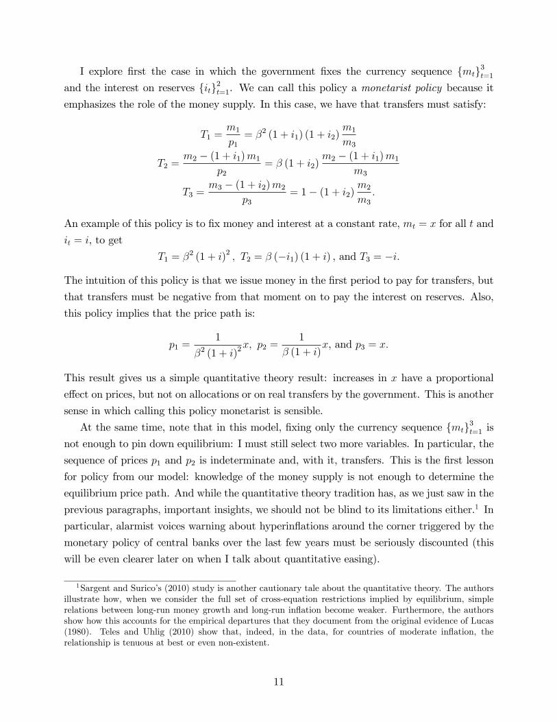
I explore first the case in which the government fixes the currency sequence {mt}3t=1and the interest on reserves {it}2t=1. We can call this policy a monetarist policy because itemphasizes the role of the money supply. In this case, we have that transfers must satisfy:

T1 =m1

p1= β2 (1 + i1) (1 + i2)

m1

m3

T2 =m2 − (1 + i1)m1

p2= β (1 + i2)

m2 − (1 + i1)m1

m3

T3 =m3 − (1 + i2)m2

p3= 1− (1 + i2)

m2

m3

.

An example of this policy is to fix money and interest at a constant rate, mt = x for all t and

it = i, to get

T1 = β2 (1 + i)2 , T2 = β (−i1) (1 + i) , and T3 = −i.

The intuition of this policy is that we issue money in the first period to pay for transfers, but

that transfers must be negative from that moment on to pay the interest on reserves. Also,

this policy implies that the price path is:

p1 =1

β2 (1 + i)2x, p2 =

1

β (1 + i)x, and p3 = x.

This result gives us a simple quantitative theory result: increases in x have a proportional

effect on prices, but not on allocations or on real transfers by the government. This is another

sense in which calling this policy monetarist is sensible.

At the same time, note that in this model, fixing only the currency sequence {mt}3t=1 isnot enough to pin down equilibrium: I must still select two more variables. In particular, the

sequence of prices p1 and p2 is indeterminate and, with it, transfers. This is the first lesson

for policy from our model: knowledge of the money supply is not enough to determine the

equilibrium price path. And while the quantitative theory tradition has, as we just saw in the

previous paragraphs, important insights, we should not be blind to its limitations either.1 In

particular, alarmist voices warning about hyperinflations around the corner triggered by the

monetary policy of central banks over the last few years must be seriously discounted (this

will be even clearer later on when I talk about quantitative easing).

1Sargent and Surico’s (2010) study is another cautionary tale about the quantitative theory. The authorsillustrate how, when we consider the full set of cross-equation restrictions implied by equilibrium, simplerelations between long-run money growth and long-run inflation become weaker. Furthermore, the authorsshow how this accounts for the empirical departures that they document from the original evidence of Lucas(1980). Teles and Uhlig (2010) show that, indeed, in the data, for countries of moderate inflation, therelationship is tenuous at best or even non-existent.

11

I explore now the case in which the government fixes the transfer sequence {Tt}3t=1 andthe interest on reserves {it}2t=1 and let money accommodate these choices. It is still the casethat by the budget constraints:

T1 = β2 (1 + i1) (1 + i2)m1

m3

T2 = β (1 + i2)m2 − (1 + i1)m1

m3

T3 = 1− (1 + i2)m2

m3

.

Working on these expressions:

T3 = 1− (1 + i2)m2

m3

⇒

m2 =1− T31 + i2

m3. (4)

Then:

T2 = β (1 + i2)m2 − (1 + i1)m1

m3

= β (1 + i2)1−T31+i2

m3 − (1 + i1)m1

m3

= β (1− T3)− β (1 + i1) (1 + i2)m1

m3

gives us

m1 =β (1− T3)− T2β (1 + i1) (1 + i2)

m3. (5)

Finally,

T1 = β2 (1 + i1) (1 + i2)m1

m3

= β2 (1− T3)− βT2 (6)

That is, we can implement this policy with any choice of m3 as long as (4), (5), and (6) are

satisfied. Note that there is a linear relation between T1, T2, and T3.

This constraint on government actions is not a surprise, but just a consequence of the

neutrality of money. By doubling the supply of money we double prices, and hence the

government cannot generate further real resources to transfer. That is, when the government

is picking transfers, it can only select two of them. In that way, if I set it = i and:

T1 = β2 (1 + i)2 , T2 = β (1 + i) (−i) , and T3 = −i

then any mt = x will implement that policy.

12

From this discussion, we obtain our second important lesson: there is no real separa-

tion between fiscal and monetary policy. As I emphasized in the introduction, at a very

fundamental level, monetary policy is always fiscal policy (and conversely, fiscal policy is

always a monetary policy). The intimate link between the two policies is given by the budget

constraint of the government. Of course, as we learned from Sargent and Wallace (1981),

different protocols about which policies are chosen first and which policies follow will give

us different predictions for the model, but determining which of these protocols is the best

framework for thinking about actual economic policy is a job for empirical evidence. Theory

can only reiterate the intimate link between fiscal and monetary policy.

3. Enriching the Model: Public Debt

Now that we understand the basic behavior of the model, I will introduce real public debt,

dt. This will let us think about many classical results in monetary theory. Also, assum-

ing that we are dealing with real debt instead of nominal debt is indifferent, as we have a

model with complete financial markets and no uncertainty, which makes the set of allocations

implementable in one situation equal to the set in the other one.

The model is unchanged except for the presence of public debt, which is sold at a price

qt. Therefore, the budget constraints of the household are now:

p1c1 +m1 + p1q1d1 +b1R1

= p1w1l1 + p1T1

p2c2 +m2 + p2q2d2 +b2R2

= p2w2l2 + (1 + i1)m1 + p2d1 + b1 + p2T2

p3c3 +m3 = p3w3l3 + (1 + i2)m2 + p3d2 + b2 + p3T3

and for the government:

m1 + p1q1d1 = p1T1

m2 + p2q2d2 = p2T2 + (1 + i1)m1 + p2d1

m3 = p3T3 + (1 + i2)m2 + p3d2.

The first-order conditions for the household are the same as before except that now:

λtptqt = βλt+1pt+1

13

for t ∈ {1, 2}. Since1

ct= −λtpt

I get:

qt = βctct+1

and since

Rt =1

β

ct+1ct

pt+1pt

I have the non-arbitrage condition:

Rt =1

qt

pt+1pt

.

Also, note that, in equilibrium, it will still be the case that:

ct = yt = lt = wt = 1 for t ∈ {1, 2, 3}

and, therefore,

qt = β for t ∈ {1, 2}

that is, the price of the debt is just equal to the discount factor (or equivalently, the return

of the debt must be equal to the real interest rate). Prices will still be given by:

p1 =1

β2 (1 + i1) (1 + i2)m3

p2 =1

β (1 + i2)m3

p3 = m3.

In the interest of space, I will skip the definition of equilibrium. However, we can highlight

how the presence of debt, by itself, does not change the equilibrium price path, which will

still depend only on the sequence of money and interests on reserves. This invariance of the

price path with respect to the presence of public debt is, at a fundamental level, the kernel

of all our results below.

3.1. Fixing Money or Fixing Transfers (Revisited)?

I can now repeat the argument about the degrees of freedom of the government for picking

policy. Given the equilibrium, the government fixes seven elements of the policy {mt, Tt}3t=1and {it, dt}2t=1 and finds the other three through the budget constraints. That is, the govern-ment has 2 more degrees of freedom than in the model without public debt.

14

For example, if the government fixes the currency sequence {mt}3t=1 and the debt andinterest sequence {it, dt}2t=1, then:

T1 = β2 (1 + i1) (1 + i2)m1

m3

+ βd1

T2 = β (1 + i2)m2 − (1 + i1)m1

m3

− d1 + βd2

T3 = 1− d2 − (1 + i2)m2

m3

Now, given some currency sequence {mt}3t=1 and the debt and interest sequence {it, dt}2t=1, I

get an allocation

ct = yt = lt = wt = 1 for t ∈ {1, 2, 3}

with prices:

p1 =1

β2 (1 + i1) (1 + i2)m3

p2 =1

β (1 + i2)m3

p3 = m3

At the cost of some algebra, I can go in the opposite direction and show how we can find

a currency sequence {mt}3t=1 from {Tt}3t=1 and {it, dt}

2t=1. To see this, note that we will still

have:

T1 = β2 (1 + i1) (1 + i2)m1

m3

+ βd1

T2 = β (1 + i2)m2 − (1 + i1)m1

m3

− d1 + βd2

T3 = 1− d2 − (1 + i2)m2

m3

.

Then, from the last equation:

m2 =1− T3 − d21 + i2

m3

and:

T2 = β (1 + i2)1−T3−d21+i2

m3 − (1 + i1)m1

m3

− d1 + βd2

= β (1− T3 − d2)− β (1 + i1) (1 + i2)m1

m3

− d1 + βd2

15

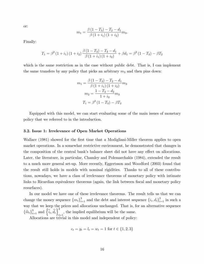
or:

m1 =β (1− T3)− T2 − d1β (1 + i1) (1 + i2)

m3.

Finally:

T1 = β2 (1 + i1) (1 + i2)β (1− T3)− T2 − d1β (1 + i1) (1 + i2)

+ βd1 = β2 (1− T3)− βT2

which is the same restriction as in the case without public debt. That is, I can implement

the same transfers by any policy that picks an arbitrary m3 and then pins down:

m1 =β (1− T3)− T2 − d1β (1 + i1) (1 + i2)

m3

m2 =1− T3 − d21 + i2

m3

T1 = β2 (1− T3)− βT2

Equipped with this model, we can start evaluating some of the main issues of monetary

policy that we referred to in the introduction.

3.2. Issue 1: Irrelevance of Open Market Operations

Wallace (1981) showed for the first time that a Modigliani-Miller theorem applies to open

market operations. In a somewhat restrictive environment, he demonstrated that changes in

the composition of the central bank’s balance sheet did not have any effect on allocations.

Later, the literature, in particular, Chamley and Polemarchakis (1984), extended the result

to a much more general set-up. More recently, Eggertsson and Woodford (2003) found that

the result still holds in models with nominal rigidities. Thanks to all of these contribu-

tions, nowadays, we have a class of irrelevance theorems of monetary policy with intimate

links to Ricardian equivalence theorems (again, the link between fiscal and monetary policy

resurfaces).

In our model we have one of these irrelevance theorems. The result tells us that we can

change the money sequence {mt}3t=1 and the debt and interest sequence {it, dt}2t=1 in such a

way that we keep the prices and allocations unchanged. That is, for an alternative sequence

{mt}3t=1 and{it, dt

}2t=1, the implied equilibrium will be the same.

Allocations are trivial in this model and independent of policy:

ct = yt = lt = wt = 1 for t ∈ {1, 2, 3}

16

and the same for real prices

qt = β for t ∈ {1, 2}wt = 1 for t ∈ {1, 2, 3}

or the nominal interest rate (conditional on a price level)

Rt =1

β

ct+1ct

pt+1pt

for t ∈ {1, 2}

so I may as well forget about them. So, to prove our point, we only need to check prices and

the budget constraint of the government. But if I set:

m3 = m3

it = it for t ∈ {1, 2}

a direct inspection of the price sequence shows that we are done.

Now, we can go to the budget constraints of the government:

m1 + p1βd1 = p1T1

m2 + p2βd2 = p2T2 + (1 + i1) m1 + p2d1

m3 = p3T3 + (1 + i2) m2 + p3d2

and pick any alternative{mt, dt

}2t=1

and{Tt

}3t=1

that satisfy those equations.

For example, I can make

m1 = γm1

for γ > 1 and T1 = T1, T3 = T3, d2 = d2, and m2 = m2. With these choices:

m3 = p3T3 + (1 + i2)m2 + p3d2

is automatically satisfied. Then, I pick

d1 =1

βT1 −

γ

β

m1

p1=1

βT1 − γβ (1 + i1) (1 + i2)

m1

m3

and:

T2 = β (1 + i2)m2 − (1 + i1) γm1

m3

+ βd2 −1

βT1 + γβ (1 + i1) (1 + i2)

m1

m3

and we complete our task.

17

Another interesting policy is to keep transfers unchanged and set m1 = γm1 for γ > 1.

Then, we still have

d1 =1

βT1 − γβ (1 + i1) (1 + i2)

m1

m3

but now:

m2 + p2βd2 = p2T2 + (1 + i1) γm1 + p2

(1

βT1 − γβ (1 + i1) (1 + i2)

m1

m3

)⇒

β (1 + i2)

m3

m2 + βd2 = T2 + γβ (1 + i2) (1 + i1)m1

m3

+

(1

βT1 − γβ (1 + i1) (1 + i2)

m1

m3

)⇒

β1 + i2m3

m2 + βd2 = T2 +1

βT1

and

(1 + i2) m2 + p3d2 = m3 − p3T3 ⇒1 + i2m3

m2 + d2 = 1− T3

and we get:

1 + i2m3

m2 + d2 =1

βT2 +

1

β2T1

1 + i2m3

m2 + d2 = 1− T3

which clearly implies again:

T1 = β2 (1− T3)− βT2

that is, any combination of m2 and d2 that is feasible in the sense of satisfying the previous

equation delivers the same sequences of allocations and prices. Note that this restriction

defines an equivalence class of alternative policies with many members.

There is a well-defined sense in which we can think about these alternative policies as

an open market operation: the government issues more currency and reduces its outstanding

debt (or takes claims against the private sector if d1 < 0). However, this operation does not

have any impact, either real or nominal. All of the changes in the government’s portfolio

(either in size or in composition) are immediately undone by an equivalent contrary action

by the household that leaves the equilibrium unchanged. However, the irrelevance of open

market operations does not imply, as sometimes erroneously interpreted, that monetary policy

is useless: the government is still determining the price level through the sequence of {it}2t=1and m3.

18

Also changes in the government’s portfolio between currency and public debt do not have

any impact on the yield curve. Remember the interest rate for the bond issued in period 1

R1 =1

β

p2p1

and for the bond issued in period 2

R2 =1

β

p3p2.

Then, the yield of a two-period bond issued at time 1 is:

R1,2 = (R1R2)0.5 = ((1 + i1) (1 + i2))

0.5

and the yield spread s1 = R1,2 −R1 = ((1 + i1) (1 + i2))0.5 − 1 + i1 is obviously unchanged.

The main result can be easily extended to the case in which we have long-lived debt and

real debt instead of nominal debt (Peled, 1985). Some (boring) algebra will deliver the result

that, again, prices, yields, and allocations are unchanged when we rebalance the central bank

portfolio’s.2

This finding delivers a very negative assessment of the prospects of quantitative easing

as an instrument of monetary policy. As long as the central bank is exchanging one type

of asset for another for which a well-working market exists, the prices of those assets (and

the implied yields) cannot change. The explanation is simple. The price of an asset is given

by the expectation of its return times the pricing kernel of the economy. Since asset returns

do not change regardless of whether the asset is held in the private or the public sector, the

only way in which the price of the asset can change is if the pricing kernel varies due to

quantitative easing. In our model, the pricing kernel is independent of the central bank’s

action, so the whole point is moot. In richer models without our classical dichotomy, the

pricing kernel will not be affected because the risk represented by the asset bought or sold

by the central bank does not disappear from the economy, it is just moved from one agent to

the other. But as long as the stand-in household needs to consider a consolidated view of its

own balance sheet and the government’s balance sheet (since this latter one will determine

future net taxes), the transfer of risk within the economy will be cancelled out.

At this level of generality in the discussion, however, we cannot rule out models in which

the transfer of risk could potentially induce changes in behavior and hence in the pricing

kernel. Think, for instance, about models with financial constraints. The key is that one

2There is also a sense in which this result vindicates the old “Real Bills doctrine”: as long as the monetaryauthority discounts at the right interest rate, it does not matter how many of the (sound) private bills itdiscounts. See Sargent and Wallace (1982).

19

needs to work hard to break the irrelevance of quantitative easing, and even when one can

do so, (see Cúrdia and Woodford, 2010, for a recent example), the results are of second

order. This result resembles the negative results in models with financial frictions, where

even very tight constraints deliver disappointingly little bang for the buck in quantitative

terms (Krueger and Lustig, 2006, is a good example of this literature).

We have, therefore, our third result: quantitative easing is unlikely to have much effect.

Up to a first-order approximation, the size and composition of the central bank’s balance

sheet are irrelevant for equilibrium prices and allocations.

There is also a growing empirical literature that attempts to measure the possible effects

of quantitative easing. See, for instance, Doh (2010), Greenwood and Vayanos (2010), or

Hamilton and Wu (2010). While the authors of these papers usually take a more positive

attitude toward quantitative easing than I do, my personal reading of their findings is that

even very large purchase programs have rather limited effects. For example, Hamilton andWu

(2010) predict a 17-basis-point effect from moving $400 billion from short to long maturities

of U.S. Treasuries.

However, this clear theoretical result and the somewhat disappointing empirical findings

raise two questions. First, why did the Fed engage in purchasing $1.25 trillion of agency

mortgage-backed securities (MBS) between January 5, 2009 and March 31, 2010? A quick

answer is that the purchase of MBS was not quantitative easing in the traditional sense, but

“credit easing,”that is, engaging in a market in which, because of a number of asymmetric

information problems, liquidity had disappeared. The Fed was not doing anything more than

being the proverbial agent with “deep pockets”agent that we include in our standard papers

in finance to ensure a lack of arbitrage opportunities. Here is not the place to analyze the

impact of the MBS purchase program except to indicate that, as a response to unusually

severe disruptions of credit markets, a monetary authority may be able to restore liquidity.

But this is very different from the management of aggregate demand through changes in the

interest rates defended by supporters of quantitative easing.

The second question is why did the Fed signal to the markets during the fall of 2010 that

it may engage in a second round of quantitative easing? The explanation, I am afraid, goes

beyond what we can examine with my model. A plausible explanation may be that even if

the Fed is aware of the second-order effects of quantitative easing, such a program may shield

the institution, at a relatively low cost, from further erosions of its independence at a time

when populist sentiments are brewing. An alternative, and somewhat more optimistic, view

is that by engaging in a cunning purchase program of U.S. Treasury debt, the Fed is trying

to lock itself into a portfolio that will suffer large capital losses if inflation is not temporarily

high during the next few years. This “commitment device”would signal to the market that

20

the implicit promise of the Fed of allowing inflation to recover over time after several years of

zero growth is credible and reducing, in that way, the real interest rates implied by the zero

nominal bound with which we currently live.

3.3. Issue 2: Some Unpleasant Monetarist Arithmetic

Sargent and Wallace (1981) highlighted that, if we take fiscal policy as given, a choice for

lower inflation today is also an implicit choice for higher inflation tomorrow. A similar type

of result shows up in our environment. Remember that in our model, inflation is given by:

p2p1= β (1 + i1)

andp3p2= β (1 + i2) .

Now, we take as given the transfer sequence {Tt}3t=1 and the debt and interest sequence{it, dt}2t=1 and we will construct a new sequence

{it, dt

}2t=1

keeping fixed {Tt}3t=1 and withthe same allocation, lower inflation between t = 1 and 2 and higher inflation between t = 2

and 3.

Using the same reasoning as before, we only need to check prices and the budget constraint

of the government. I start by picking i1 < i1 and i2 > i1 such that

(1 + i1) (1 + i2) =(1 + i1

)(1 + i2

).

I also pick m3 = m3. These choices deliver the result that p1 = p1 and p3 = p3 and that there

is less inflation in the alternative equilibrium in the first period and more in the second.

Finally, note that:

T1 = β2(1 + i1

)(1 + i2

) m1

m3

+ βd1

T2 = β(1 + i2

) m2 −(1 + i1

)m1

m3

− d1 + βd2

T3 = 1− d2 −(1 + i2

) m2

m3

which still leaves us with one degree of freedom: four variables to choose (m1, m2, d1, and

d2) and three constraints. Again, we have our leitmotif of the interdependence of fiscal and

monetary policy bounding the degrees of freedom of the government.

21

3.4. Issue 3: Fiscal Theory of the Price Level

We argued before that in our model, it is not possible to build non-Ricardian policies and

that, therefore, strict versions of the fiscal theory of the price level do not hold. However,

some of the insights of that literature are still valid.

Imagine that we want to ensure that the nominal value of T1 is equal to d0 (we can easily

think about this case as some initial stock of public debt). We showed before that, once we

have fixed T2 and T3, we must have

T1 = β2 (1− T3)− βT2.

Therefore, given T2 and T3, the price level p1 must satisfy:

d0p1= β2 (1− T3)− βT2

or

p1 =d0

β2 (1− T3)− βT2which determines the price level at t = 1. This is a version of the fiscal theory of the price

level. Note that this determination of p1 happens in an economy that satisfies the quantitative

theory of money. Also, note that the government is “special”: it only satisfies the initial

condition for a particular p1, which eliminates all possible equilibria that deliver different p1.

In comparison, the household needs to satisfy its budget constraint for all equilibria. In other

words, we could force the government to satisfy its budget constraint given some nominal d0for all equilibria and we would eliminate this result (see Kocherlakota and Phelan, 1999, for

a more careful development of this point).

At the same time, we have:

p1 =1

β2 (1 + i1) (1 + i2)m3

Thus, we have the additional constraint on m3 and p3:

d0

β2 (1− T3)− βT2=

1

β2 (1 + i1) (1 + i2)m3 ⇒

p3 = m3 =β (1 + i1) (1 + i2)

β (1− T3)− T2d0

22

Since we still have the three resource constraints, the government must pick

m1 =β (1− T3)− T2 − d1β (1 + i1) (1 + i2)

m3 = 1−d1

β (1− T3)− T2d0

m2 =1− T3 − d21 + i2

m3 =β (1 + i1) (1− T3 − d2)

β (1− T3)− T2d0

(the third one is automatically satisfied by our definition of T1). The government then selects

{it, dt}2t=1 and we have our complete equilibrium.

3.5. Issue 4: Zero Lower Bound on Nominal Interest Rates

I argued before that in this model, given our assumptions, there is no particular diffi culty

in thinking about Rt < 1. However, it is also instructive to eliminate that possibility and

call back the “stuffi ng-in-your-matress”technology that allows households to hold their cash

balances instead of depositing them at the central bank. If Rt = 1, then households are

indifferent between both choices (I still assume that households do not face any storage cost,

such as the installation of an alarm system at home to prevent their cash from being stolen).

The key to understanding what happens when we have a zero lower bound on nominal

interest rates is to realize that the Euler equation for the household is still:

Rt =1

β

ct+1ct

pt+1pt

regardless of whether the zero bound binds because financial markets are complete and the

household has access to them. Also, it will still be the case that ct = 1 for all t (the classical

dichotomy holds), and hence:

Rt =1

β

pt+1pt

If, for instance, β > 1 (think about it as a situation where we get a negative demand shock),

and Rt = 1, the only way in which we can have an equilibrium is if pt+1 > pt. Fortunately,

this is what our other equilibrium conditions deliver. Remember that

p1 =1

β2 (1 + i1) (1 + i2)m3

p2 =1

β (1 + i2)m3

p3 = m3

23

and if β > 1, and Rt = 1 (and by non-arbitrage, i1 = i2 = 0):

p1 =m3

β2

p2 =m3

β

p3 = m3

which is exactly what we need to get the Euler equation to hold. In other words, a discount

factor bigger than 1 just generates an inflation exactly equal to it:

p3p2=p2p1= β

How can we reconcile this inflationary path created by the zero bound on the nominal interest

rate with the usual argument that the zero bound may induce a deflationary black-hole? Here

is a particular situation in which the presence of nominal rigidities makes a radical difference.

When we have price rigidities, future prices cannot adjust as fast as we would need to clear

the savings market (as it happens in our benchmark model). The only way in which we

can clear markets is with a fall in output, which reduces the desired level of saving and

with it, makes the Euler equation hold. In a world with nominal rigidities, where output

is partially demand-determined, this is achieved with a fall in aggregate demand triggered

by a deflationary path: deflation increases real interest rates, which reduces current demand

and, with it, output and total savings, and ensures market clearing. It is not the zero lower

bound that creates a problem. It is the interaction between the zero lower bound and nominal

rigidities.

4. A Model with Government Consumption and Distortionary Tax-

ation

I will now switch gears and analyze the effects of government consumption and distortionary

taxation in an environment very similar to the one we just used. Again, this emphasizes the

usefulness of modern dynamic macroeconomics in thinking through current policy debates.

I will proceed through the analysis in two steps. First, in this section, I will eliminate

money (and the policy instruments associated with it), since the main issues I want to discuss

do not depend on the presence of money. Second, I would have only two periods, t ∈ {1, 2},since two periods are all I need to make my points.

I will still have a stand-in household that picks consumption ct and labor supply lt to

24

maximize:

log c1 −l212+ β

(log c2 −

l222

)The unitary Frisch elasticity of these preferences will be surprisingly useful below.

The budget constraints are now:

c1 +b1R1

= (1− τ 1)w1l1 + T1

c2 = (1− τ 2)w2l2 + b1 + T2

where we introduce, as new notation, τ t as the tax rate on labor income. I do not tax the

returns on public debt because, in equilibrium, the returns would increase exactly by the

quantity required to offset the tax. For fiscal policy, the tax on labor is the most important

novelty of the model with respect to the framework of the previous sections. Since we do not

have money, I have eliminated prices from the budget constraints and expressed all quantities,

including public debt b1, in real terms.

I will keep the technology constant and the final good is still produced by a competitive

firm with a linear technology yt = lt. Again, this is just a simple way to fix wages over time

without having to worry about physical capital or curvatures of labor supply.

The government uses its revenue from lump-sum transfers from the household and taxes

on labor income to finance government consumption, g, in period 1. To simplify, the gov-

ernment does not consume in the second period and g is dumped into the sea (or, more

palatably, it enters into the utility function of the representative household in a separable

way). A simple way to think about this is that we are concerned only about the effects of

increasing government consumption over some long-run average, and hence, we are normal-

izing all variables to get rid of the average level of public consumption (in section 5, I will let

government consumption be positive in all periods at the cost of more algebra). Thus, the

government budget constraints are:

g + T1 = τ 1w1l1 +b1R1

b1 + T2 = τ 2w2l2.

It will be more convenient below to use the consolidated budget constraint:

g = τ 1w1l1 − T1 +τ 2w2l2 − T2

R1

25

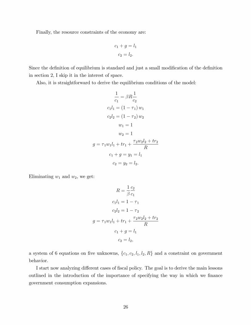
Finally, the resource constraints of the economy are:

c1 + g = l1

c2 = l2.

Since the definition of equilibrium is standard and just a small modification of the definition

in section 2, I skip it in the interest of space.

Also, it is straightforward to derive the equilibrium conditions of the model:

1

c1= βR

1

c2

c1l1 = (1− τ 1)w1c2l2 = (1− τ 2)w2

w1 = 1

w2 = 1

g = τ 1w1l1 + tr1 +τ 2w2l2 + tr2

R

c1 + g = y1 = l1

c2 = y2 = l2.

Eliminating w1 and w2, we get:

R =1

β

c2c1

c1l1 = 1− τ 1c2l2 = 1− τ 2

g = τ 1w1l1 + tr1 +τ 2w2l2 + tr2

R

c1 + g = l1

c2 = l2,

a system of 6 equations on five unknowns, {c1, c2, l1, l2, R} and a constraint on governmentbehavior.

I start now analyzing different cases of fiscal policy. The goal is to derive the main lessons

outlined in the introduction of the importance of specifying the way in which we finance

government consumption expansions.

26

4.1. Case 1: No Government Consumption

We start with the simplest case of g = 0 to have a baseline case. Then, τ 1 = τ 2 = tr1 =

tr2 = d = 0 and the equilibrium conditions simplify to

R =1

β

c2c1

c1l1 = 1

c2l2 = 1

c1 = l1

c2 = l2

or l1 = l2 = c1 = c2 = 1 and R = 1β.

This is pretty much the same equilibrium as the one in the model with money, consumption

and labor are constant over time, and the real interest rate is the inverse of the discount factor.

4.2. Case 2: Government Expansion, Lump-sum Financed

We explore now the case g > 0, but all government consumption is financed through lump-

sum taxes (τ 1 = τ 2 = 0). We can think about this exercise as exploring the case of an

expansionary fiscal policy with respect to the baseline g = 0.

The equilibrium conditions are now:

R =1

β

c2c1

c1l1 = 1

c2l2 = 1

g = tr1 +tr2R

c1 + g = l1

c2 = l2.

Then c1 = l1 − g and(l1 − g) l1 = 1⇒ l21 − gl1 − 1 = 0

27

which implies that:

l1 =g +

√g2 + 4

2

c1 =

√g2 + 4− g2

l2 = 1

c2 = 1

R =1

β

2√g2 + 4− g

tr1 + β

√g2 + 4− g2

tr2 = g

(we have kept the positive root of l1).

It is interesting to point out two remarks:

1. g > 0 expands output in period 1 with respect to the case g = 0. Note that

y1 = l1 =g +

√g2 + 4

2>g +

√g2 + 4− 2g2

=g +

√(2− g)2

2= 1

Also, since for small g √g2 + 4

2≈ 1

the increase in output with respect to the baseline case is approximately half of the

increase in g. Thus, by the resource constraint, c1 falls. Output in period 2 is unchanged.

It is quite remarkable that the size of this multiplier is the range of values obtained by

more involved dynamic models (for example, if we had capital). The reason labor supply

goes up is that there is a negative wealth effect triggered by higher taxes. The interest

rate R increases to induce the representative household to consume less in period 1 to

satisfy the resource constraint.

2. The timing of lump-sum transfers is irrelevant: d does not appear in the equilibrium

conditions and we can pick any combination of tr1 and tr2 as long as it satisfies:

tr1 + β

√g2 + 4− g2

tr2 = g.

In other words, it does not matter if we finance the government expansion with more

taxes today and a balanced budget or with debt and deficit. This is, of course, just the

28

Ricardian equivalence. Note, however (and this should be clear), that the Ricardian

equivalence does not say that an expansion of government expenditure does not have

any effect when we have lump-sum taxes. We still have an increase in output. What the

Ricardian equivalence says is that whether we finance that expansion with lump-sum

taxes today or tomorrow is irrelevant.

Finally, an obvious point about welfare that is, however, often forgotten. The increase in

output does not translate necessarily into an increase in welfare. In this economy gt is useless

and since the impact multiplier is smaller than 1, consumption and leisure fall and with them

welfare. In a richer model, where gt enters into the utility function, the net outcome will

depend on the parameter weighting gt in the preferences.

4.3. Case 3: Government Expansion, Distortionary Taxes Today

We explore the case g > 0 financed through distortionary taxes in the first period (τ 1 > 0,

τ 2 = 0) and, to simplify the expressions, no lump-sum transfers.

The equilibrium conditions are now:

R =1

β

c2c1

c1l1 = 1− τ 1c2l2 = 1

g = τ 1l1

c1 + g = l1

c2 = l2.

Then:

1− τ 1 = 1−g

l1= 1− l1 − c1

l1=c1l1

and:

c1l1 =c1l1⇒ l1 = 1

which implies that:

c1 = 1− gτ 1 = g

c2 = l2 = 1

29

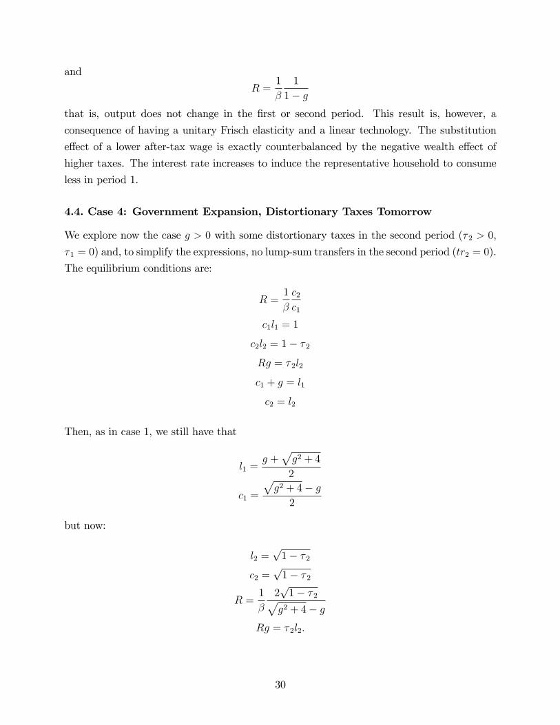
and

R =1

β

1

1− gthat is, output does not change in the first or second period. This result is, however, a

consequence of having a unitary Frisch elasticity and a linear technology. The substitution

effect of a lower after-tax wage is exactly counterbalanced by the negative wealth effect of

higher taxes. The interest rate increases to induce the representative household to consume

less in period 1.

4.4. Case 4: Government Expansion, Distortionary Taxes Tomorrow

We explore now the case g > 0 with some distortionary taxes in the second period (τ 2 > 0,

τ 1 = 0) and, to simplify the expressions, no lump-sum transfers in the second period (tr2 = 0).

The equilibrium conditions are:

R =1

β

c2c1

c1l1 = 1

c2l2 = 1− τ 2Rg = τ 2l2

c1 + g = l1

c2 = l2

Then, as in case 1, we still have that

l1 =g +

√g2 + 4

2

c1 =

√g2 + 4− g2

but now:

l2 =√1− τ 2

c2 =√1− τ 2

R =1

β

2√1− τ 2√

g2 + 4− gRg = τ 2l2.

30

Clearly, l2 < 1. Also we have:

1

β

2√1− τ 2√

g2 + 4− gg = τ 2

√1− τ 2 ⇒ τ 2 =

1

β

2g√4 + g2 − g

and:

l2 = c2 =

√1− 1

β

2g√4 + g2 − g

and:

R =1

β

2√1− 1

β2g√4+g2−g√

4 + g2 − g.

This is an expression on the order of√g, that is, the effects on the second period allocation

are a square root of the increase in government consumption. This is why, for small g, it does

not really matter much to distinguish between debt-financed or lump-sum-transfer-financed

fiscal expansions. Labor supply goes up in the first period because of the negative wealth

effect and goes down in the second period because of the distortionary effect of taxes on

wages.

4.5. Lessons

In summary:

1. When the increase in government consumption today is financed through lump-sum

transfers (either today or tomorrow), output increases in the first period and stays the

same in the second period. The increase in output in the first period is approximately

half of the increase in government consumption.

2. When the increase in government consumption today is financed through lump-sum

transfers, it is irrelevant if we tax today or tomorrow (Ricardian equivalence).

3. When the increase in government consumption today is financed through distortionary

taxes today, output is unchanged in both periods.

4. When the increase in government consumption today is financed through distortionary

taxes tomorrow, output increases today, approximately by half of the increase in gov-

ernment consumption, and falls in the second period, approximately by the square root

of the increase in government consumption.

While some of the details of these lessons depend on our particular functional forms, the

main thrust of the results will go through in a much wider set of environments. In particular,

31

the idea that the effectiveness of expansionary fiscal policy depends crucially on the way it

is financed appears clearly even in the most sophisticated DSGE models. Similarly, many of

the orders of magnitude from 1 to 4 are a good indication of the results we should expect

from medium-scale estimated models such as those described in Fernández-Villaverde (2010).

5. Putting it All Together

Now, as a capstone of the paper, I will put together monetary and fiscal policy in a coherent

framework. For that, I return to a three-period model and reintroduce money but I keep the

distortionary taxes and government consumption of the previous section in all three periods.

For lack of a better name, I will call this environment the unified model.

5.1. Environment

There is a stand-in household that picks consumption ct, labor supply lt, and real money

holdings to maximize

log c1 −l212+ β

(log c2 −

l222

)+ β2

(log c3 −

l232+ log

m3

p3

)subject to:

p1c1 +m1 + p1q1d1 +b1R1

= (1− τ 1) p1w1l1 + p1T1

p2c2 +m2 + p2q2d2 +b2R2

= (1− τ 2) p2w2l2 + (1 + i1)m1 + p2d1 + b1 + p2T2

p3c3 +m3 = (1− τ 3) p3w3l3 + (1 + i2)m2 + p3d2 + b2 + p3T3.

The technology side stays as before, where the final good is produced by a competitive firm

with a linear technology yt = lt.

The government budget constraints are:

m1 + τ 1p1w1l1 + p1q1d1 = p1g1 + p1T1

m2 + τ 2p2w2l2 + p2q2d2 = p2g2 + p2T2 + (1 + i1)m1 + p2d1

m3 + τ 3p3w3l3 = p3g3 + p3T3 + (1 + i2)m2 + p3d2

and the aggregate resource constraint ct+gt = lt for all t ∈ {1, 2, 3} . It is trivial to check that,by consolidating the budget constraints of the household and the government and imposing

the market clearing conditions b1 = b2 = 0 and w1 = w2 = w3 = 1, we recover the aggregate

32

resource constraint. Again, the definition of equilibrium is straightforward and I omit it to

save space. Also, to ease notation, I will already have applied the result w1 = w2 = w3 = 1

in my next derivations.

5.2. Solving for the Equilibrium

The Lagrangian of the household is given by

log c1 −l212+ β

(log c2 −

l222

)+ β2

(log c3 −

l232+ log

m3

p3

)+λ1

(p1c1 +m1 + p1q1d1 +

b1R1− (1− τ 1) p1l1 − p1T1

)+βλ2

(p2c2 +m2 + p2q2d2 +

b2R2− (1− τ 2) p2w2l2 − (1 + i1)m1 − p2d1 − b1 − p2T2

)+β2λ3 (p3c3 +m3 − (1− τ 3) p3w3l3 − (1 + i2)m2 − p3d2 − b2 − p3T3) .

The first-order conditions for the household are for all t

1

ct= −λtpt

lt = −λt (1− τ t) pt

for t ∈ {1, 2}

λt = β (1 + it)λt+1

λtptqt = βλt+1pt+1

λtRt

= βλt+1

and for t = 31

m3

= −λ3.

Using the resource constraint:

ct + gt = lt

and the first two optimality conditions, we get lt (lt − gt) = 1− τ t or:

yt = lt =gt +

√g2t + 4 (1− τ t)2

33

and

ct =

√g2t + 4 (1− τ t)− gt

2.

We can see from these two equations that output, consumption, and labor depend only on

taxes and government consumption in the current period.

Now, for the price level, we get:

p1 =1

β2 (1 + i1) (1 + i2)

m3

c1

p2 =1

β (1 + i2)

m3

c2

p3 =m3

c3

for the public debt in t ∈ {1, 2}:qt = β

ctct+1

and for the nominal interest rate in t ∈ {1, 2}:

Rt =1

β

ct+1ct

pt+1pt

.

We summarize the results

yt = lt =gt +

√g2t + 4 (1− τ t)2

for t ∈ {1, 2, 3}

ct =

√g2t + 4 (1− τ t)− gt

2for t ∈ {1, 2, 3}

wt = 1 for t ∈ {1, 2, 3}

p1 =1

β2 (1 + i1) (1 + i2)

m3

c1

p2 =1

β (1 + i2)

m3

c2

p3 =m3

c3

qt = βctct+1

for t ∈ {1, 2}

Rt =1

β

ct+1ct

pt+1pt

for t ∈ {1, 2}

bt = 0 for t ∈ {1, 2} .

34

As for the government constraints:

m1 + τ 1p1l1 + p1q1d1 = p1g1 + p1T1

m2 + τ 2p2l2 + p2q2d2 = p2g2 + p2T2 + (1 + i1)m1 + p2d1

m3 + τ 3p3l3 = p3g3 + p3T3 + (1 + i2)m2 + p3d2

where we see the 16 policy instruments, {mt, τ t, Tt, gt}3t=1 and {it, dt}2t=1 , and hence the

presence of 13 degrees of freedom. This basically means that we have a large class of equivalent

policies that implement the same allocations.

The clearest example of these equivalent policies is, naturally, that lump-sum transfers do

not show up in the equilibrium conditions except in the three government constraints. This is

a rather direct consequence of the result that in our unified model, Ricardian equivalence still

holds. Hence, any changes in the timing of transfers will be irrelevant. At the cost of rather

boring algebra, we could characterize all these equivalent policies and show, for instance, that

quantitative easing will still be completely useless.

Also, we could explore the consequences of many different changes in government policy.

In the interest of space, I will focus on just one experiment: an expansion in government

consumption gt. Imagine, first, that such an expansion is financed with lump-sum transfers.

Then:∂yt∂gt

=1

2

(1 +

gt

(g2t + 4 (1− τ t))0.5

)Clearly, this result nests our case 2 in section 4, where τ t = 0 and for gt small, I found that

∂yt∂gt≈ 12.

Now the result with positive gt and τ t is a bit more complicated. To get an idea of the size of

the multiplier, I plot in figure 1, the multiplier for different values of gt (from 0 to 0.4) and for

three values of τ t (0.2, 0.3, and 0.4). While the value of the multiplier is not 0.5 any longer,

it stays within reasonable values (up to 0.62), which are again similar to the ones reported

in the empirical literature and the multipliers derived from richer DSGE models.

Interestingly, the multiplier never gets close to one, which implies, by the resource con-

straint of the economy, that ct falls. Hence, given that the price level in each period is given

by:

pt ∝m3

ct

an increase in gt increases pt even if the money supply and the interest rates set up by

monetary policy are unchanged.

35

Therefore, fiscal policy is the key to determining the price level and inflation even in a

fully neoclassical world such as the one presented here. Also, the price of public debt

qt = βctct+1

would fall (we need to induce the households to consume less today and that is achieved with

a higher real interest rate). However the nominal interest rate on bonds:

Rt =1

β

ct+1ct

pt+1pt

stays constant since the higher real interest rate is exactly balanced by the lower inflation

rate between period t and t+ 1.

We can move now to the case where the expansion in government consumption gt is

financed with future distortionary taxes. The impact multiplier is still given by:

∂yt∂gt

=1

2

(1 +

gt

(g2t + 4 (1− τ t))0.5

)while the effects on future output depend on when and how τ t, Tt, and mt are changed to

restore the government’s intertemporal budget constraint. The consequences for prices and

interest rates will be the same as before except for the possible consequences for ct+1.

36

Finally, in the case in which the expansion in government consumption gt is financed with

distortionary taxes today, some algebra will deliver that:

∂yt∂gt

= 0

and prices remain constant.

These derivations show us an important final lesson: we can use fiscal policy as a substitute

for monetary policy. In fact, you can show in a much more general set-up that all of the

changes in allocations that can be achieved with monetary policy can also be achieved with

fiscal policy. Correia, Nicolini, and Teles (2008), in an important recent contribution, show

that we can implement the same set of optimal allocations with fiscal instruments as with

monetary policy and, moreover, that such optimal policy is independent of the degree or type

of price stickiness.

6. Conclusion

In a learned and insightful book, Pincus (2009) has recently reminded us that the Glorious

Revolution of 1688 in England, despite its faded role in the contemporary historiographical

fashions genetically suspicious of Whiggish readings of events, was the initial milestone of

modernity, the true start of contemporary economic growth, and of open, liberal societies.

Among the many institutional changes brought about by the landing of the Prince of Orange

at Torbay, the one that concern us the most is the chartering of the Bank of England on July

27 1694, which started us on the road toward monetary policy as we currently understand it.

What is sometimes forgotten is that this first modern central bank (with the permission, of

course, of the Swedish Riksbank) was created not so much as a tool for monetary policy, but

as an instrument for fiscal policy. The position of William and Mary was tenuous. The War

of the League of Augsburg had been dragging on for 5 long years without a clear path toward

victory for the Grand Alliance, the menace of the return of James II from his French exile was

ever present, and the Battle of Beachy Head had transparently demonstrated that England

could lose control of the Channel. Money was needed and it was needed fast. A central bank,

with many privileges such as the issuing of notes, was an expedient way to raise the required

resources. As one pamphleteer of the time argued, such a bank could provide “ready money”

in case of “a sudden emergency”to “equip Armadas, supply armies, levy soldiers,”(cited by

Pincus, 2009, p. 390).

This historical detour illustrates, better than any other I can think of, the deep intercon-

nection between fiscal and monetary policy that has run through the paper. For a couple

37

of decades, from 1985 to around 2007, that interconnection was partially hidden from the

public debate. Monetary policy seemed to be just an issue of raising or lowering the nominal

interest rate at appropriate moments to stabilize the economy and achieve low inflation. But

this was the case only because fiscal policy did not impose tight constraints on what the mon-

etary authority could do and because the economy did not require large policy interventions.

Once the 2007-2009 recession broke those conditions, the intimate relation between different

policies has resurfaced.

This has important political-economic implications. In a world in which monetary policy

has a clear and rather limited set of tasks and goals, it is feasible to entertain the idea of an

independent central bank. However, once fiscal and monetary policy start to interact with

each other in dramatic ways, the pressure to achieve coordination between both of them will

mount. One possibility, witnessed at least to some degree in the U.S., is that a populist

impulse will subordinate central banks to Treasury directions, as was the case for a long

time. A second possibility, which seems closer to the European experience, is that monetary

authorities end up prevailing over those directing fiscal policy. Of course, the swing in one

direction or the other will depend crucially on the relative strengths of each institution, and

the weakness of the Fed with respect to Congress in the U.S. versus the strength of the ECB

with respect to national authorities (at least those outside Germany and France) forecasts

that these developments will become more acute over time.

But no matter what the final outcome of these political struggles is, we will still face the

need to implement optimal policies. I have tried to argue in this paper that modern dynamic

macroeconomics has uncovered some important lessons to address this challenge.

38

References

[1] Chamley, C. and H. Polemarchakis (1984). “Assets, General Equilibrium and the Neu-

trality of Money.”Review of Economic Studies, 51, 129-38.

[2] Cochrane, J. (2010). “Determinacy and Identification with Taylor Rules.”Mimeo, Uni-

versity of Chicago.

[3] Correia, I., J.P. Nicolini, and P. Teles (2008). “Optimal Fiscal and Monetary Policy:

Equivalence Results.”Journal of Political Economy 116, 141-170.

[4] Cúrdia, V. and M. Woodford (2010). “The Central-Bank Balance Sheet as an Instrument

of Monetary Policy.”NBER Working Paper 16208.

[5] Doh, T. (2010), “The effi cacy of large-scale asset purchases at the zero lower bound,”

Federal Reserve Bank of Kansas City Economic Review, Q2, 5-34.

[6] Eggertsson, G.B. and M. Woodford (2003). “The Zero Bound on Interest Rates and

Optimal Monetary Policy.”Brookings Papers on Economic Activity 34, 139-235.

[7] Fernández-Villaverde, J. (2010). “The Econometrics of DSGEModels.”SERIES: Journal

of the Spanish Economic Association 1, 3-49.

[8] Greenwood, R. and D. Vayanos (2010). “Bond supply and excess bond returns.”Mimeo,

London School of Economics.

[9] Hall, R.E. (2009a). “By How Much Does GDP Rise if the Government Buys More

Output?”Brookings Papers on Economic Activity, 2009:2, 183-231.

[10] Hall, R.E. (2009b). “Reconciling Cyclical Movements in the Marginal Value of Time and

the Marginal Product of Labor.”, Journal of Political Economy 117, 281-323.

[11] Hamilton, J. and C. Wu (2010). “The Effectiveness of Alternative Monetary Policy Tools

in a Zero Lower Bound Environment.”Mimeo, UCSD.

[12] Kocherlakota, N. and C. Phelan (1999). “Explaining the Fiscal Theory of the Price

Level.”Quarterly Review, Federal Reserve Bank of Minneapolis, Fall, 14-23.

[13] Krueger, D. and H. Lustig (2006). “When Is Market Incompleteness Irrelevant for the

Price of Aggregate Risk (and When Is It Not)?”Journal of Economic Theory 145, 1-41.

[14] Lucas, R.E. (1980). “Two Illustrations of the Quantity Theory of Money.”American

Economic Review 70, 1005-14.

39

[15] Peled, D. (1985). “Stochastic Inflation and Government Provision of Indexed Bonds.”

Journal of Monetary Economics 15, 291-308.

[16] Pincus, S. (2009). 1688: The First Modern Revolution. Yale University Press.

[17] Sargent, T.J. and P. Surico (2010). “Monetary Policies and Low-frequencyManifestations

of the Quantity Theory.”American Economic Review, forthcoming.

[18] Sargent, T.J. and N. Wallace (1981). “Some Unpleasant Monetarist Arithmetic.”Quar-

terly Review, Federal Reserve Bank of Minneapolis, Fall.

[19] Sargent, T.J. and N. Wallace (1982). “The Real Bills Doctrine versus the Quantity

Theory: A Reconsideration.”Journal of Political Economy 90, 1212-36.

[20] Teles P. and H. Uhlig (2010). “Is Quantity Theory Still Alive?”NBER Working Paper

16393.

[21] Wallace, N. (1981). “A Modigliani-Miller Theorem for Open-Market Operations.”Amer-

ican Economic Review 71, 267-74.

40