1

A Robust Algorithm for Information Hiding inDigital Pictures

by

Raymond W. Hwang

Submitted to the Department of Electrical Engineering and ComputerScience in partial fulfillment of the requirements for the degree

Master of Engineering

At the

The Massachusetts Institute of Technology

May 21, 1999

Raymond Hwang, 1999. All rights reserved.

The author hereby grants MIT permission to reproduce and distribute paperand electronic copies of this document, in whole or in part, and to grant

other the right to do so.

Author…………………………………………………………………………Department of Electrical Engineering and Computer Science

May 21, 1999

Certified by……………………………………………………………………Walter Bender

Thesis Supervisor

Accepted by…………………………………………………………………...Arthur C. Smith

Chairman, Department Committee on Graduate Theses

2

Acknowledgements

I would like to thank Walter Bender for providing me with the opportunity to participatein this research. It has been an extremely valuable educational experience. The chanceto work at the Media Laboratory, with its extraordinary people and technology, has beenmost refreshing and eye-opening.

This thesis would not have been possible without the insight and guidance of DanielGruhl. Thank you for your patience, knowledge and humor.

Thanks to Fernando Paiz, for just being around during this whole thing.

Lastly, thanks to my friends and family (Mom, Dad, and Lindi) who have accompaniedme this far.

3

A Robust Algorithm for Information Hiding in Digital Picturesby

Raymond W. Hwang

Submitted to theDepartment of Electrical Engineering and Computer Science

May 21, 1999

In Partial Fulfillment of the Requirements for the Degree ofMaster of Engineering in Electrical Engineering and Computer Science.

Abstract

A problem inherent in information hiding techniques for digital images is that ofalignment during data extraction. This alignment problem can be solved using a searchapproach where a combination of coarse orientation detection, random search andgradient descent methods are employed. When used in conjunction with the Patch Trackalgorithm, it is possible to create an information hiding and retrieval system that is robusttowards rotation, cropping and noise; successful data extraction can occur with a highdegree of certainty from scanned images, rotated images and partial images. An imagecan be encoded with a desired piece of information (a reference number, URL etc.) withPatch Track by way of pseudo-random, imperceivable alterations of intensity throughoutthe image. This information can be then be extracted by the intended parties with adecoder. Various applications exist for this watermarking system including photoannotation, verification of image ownership on the Internet and data warehousing.

Thesis Supervisor: Walter BenderTitle: Assistant Director of Information Technology, Senior Research Scientist, The MITMedia Laboratory

4

Table of Contents

1 Introduction and Research Context1.1 Introduction…………………………………………………………….61.2 Current Research……………………………………………………….9

2 Patchwork Encoding and Decoding2.1 Information Hiding Ideology…………………………………………..112.2 Mathematical Basis…………………………………………………….122.3 Encoding Mechanism…………………………………………………..162.4 Hypothesis Testing…………………………………………………..…192.5 Decoding Mechanism………………………………….……………….21

3 Encoding Algorithm Parameters3.1 Brightness………………………………………………………………253.2 Patch Encoding…………………………………………………………263.3 Patch Size……………………………………………………………….283.4 Patch Shape……………………………………………………………..283.5 Number of Patches…………………………………………………..….283.6 Patch Intensity and Contour…………………………………………….293.7 Visibility Mask………………………………………………………….30

4 Orientation Detection and Correction4.1 Motivation……………………………………………………………….334.2 Implementation………………………………………………………….35

5 Improved Decoding by Gradient Search5.1 Motivation………………………………………………………………395.2 Gradient Descent………………………………………………………..395.3 Advantages and Implementation of Random Search/Gradient Descent..42

6 Multiple Bit Encoding/Decoding6.1 Implementation………………………………………………………….476.2 Error Correction…………………………………………………….…...47

7 Conclusion7.1 Conclusion………………………………………………………………50

References………………………………………………………………….…….52

Appendix A, encode.c…………………………………………………………...53Appendix B, decode.c…………………………………………………………...63Appendix C, odetect.c…………………………………………………………...66Appendix D, grad.c……………………………………………………………...82Appendix E, mbencode.c………………………………………………………..101Appendix F, mbdecode.c………………………………………………………..114

5

Table of Figures

Figure 2.1: Bender Buck in 8-bit Grayscale…………………………………….13Figure 2.2: Expected S10,000 Distribution for a Bender Buck, σ=10,400……….16Figure 2.3a: Encoded Bender Buck……………………………………………..18Figure 2.3b: Original Unencoded Bender Buck………………………………...19Figure 2.4: Hypothesis Test for an Image when Sn > Threshold ……………….20Figure 2.5: Hypothesis Test for an Image when Sn < Threshold ……………….20Figure 2.6a: Encoded Bender Buck with Points of Encoding Visualized………25Figure 2.6b: The Decode Window for Figure 2.6a with Decoding Points

Visualized……………………………………………………………………22Figure 2.6c: Decode Window Misaligned Due to Rotation……………………..22Figure 2.7: A Bender Buck with n=10,000 and δ=10………..………….……...23Figure 2.8: Sn Values Obtained From Decoding Figure 2.7…………………….23

Figure 3.1: Bender Buck Encoded with n=10,000 and δ=80…………………...26Figure 3.2: Visualization of Patches……………………………………………..27Figure 3.3: Bender Buck Encoded with n=15,000, δ=80 and radius of 10……..29Figure 3.4: Side View of Pseudo-Randomly Filled Circle………………………29Figure 3.5: Side View of a Negative Random Cone…………………………….30Figure 3.6: Block Diagram of the Double Sinc Blur Technique………………...31

Figure 4.1: One-bit Quantized Image Using a Brightness Threshold of 167……36

Figure 5.1: Perfect Decode Window Orientation………………………………..40Figure 5.2: Imperfect Decode Window Orientation……………………………..40Figure 5.3: Misleading Points Used in Calculating the Gradient………………..41Figure 5.4: Scanned Image of the Cut, Encoded Bender Buck……………….…44Figure 5.5: Aligned Bender Buck Using Random Search and Gradient

Descent……………………………………………………………………....45Figure 5.6: Entire Bender Buck Before Random Search and Gradient Descent...45

Figure 6.1: “0,1,1,0” Sn Values Under Error Correction Scheme……………….48

6

Chapter 1:

Introduction and Historical Background

1.1 IntroductionThe emergence of the Internet as a popular means of communication has introduced new

dilemmas regarding intellectual property. Certainly, the wide proliferation of URLs in

print and television advertisements provides evidence towards the general popularity of

this medium. It is common to find corporations and organizations offering web sites that

complement other forms of advertising and publicity, providing consumers with vast

amounts of company and product information, services and support. Publishing

electronically disseminates information quickly and extensively, but given the nature of

the World Wide Web, copyright protection is infringed upon with greater ease and/or

frequency than with printed documents. This phenomenon can be attributed to the fact

that text and images that exist in electronic form can easily be duplicated and republished

without degradation, attribution and often without detection. It can be difficult to find

such offenses when they occur because of the vast size of the Internet. And when such

cases are found, it can be hard to prove ownership. A second problem also exists: with

the advent of high-quality desktop printers, such images can be used offline as well,

adding to the extent of the problem.

These problems exist because current popular formats for images on the Internet do not

allow for any type of proprietary protection. Common Internet image formats, such as

GIF1, do not contain provisions for copyright. TIFF2 and JPEG3, are compression

techniques that have “out of band” provisions that place copyright information in

1 Graphic Interchange Format2 Tagged Image File Format3 Joint Photographic Experts Group

7

headers. This mechanism for copyright protection is not robust in that such copyright

notifications can be manually removed with ease. Also, printing such images results in

the loss of these headers. When a JPEG image is printed out and scanned back into

digital form, header lines that were present in the original file will not be present in the

scanned file. Any copyright information contained in the original image is therefore lost.

Without more robust copyright mechanisms, everyday users have come to regard images

that appear on the Internet as being in the public domain and therefore utilize them as

such without malicious intent. Because of this belief, it is common to find the same

picture or icon on multiple sites. But who was the photographer for this particular picture

or which artist designed that icon? Do these images appear with permission or

attribution? More often than not, these images do not appear with any reference or

compensation to their originators. For both the corporation and the artist, this trend is not

an appealing aspect of publishing on the Web.

This dilemma was one of the motivating factors for the research described in this thesis.

One possible solution to this problem can be achieved with digital watermarking. The

Patch Track algorithm, a multiple-bit extension of the Patchwork4 technique, discussed

below, allows users to watermark images with selected data (such as an identification

number) in a manner that is imperceivable to human eyes while being robust to noise,

rotation and cropping. These characteristics make the Patch Track algorithm a good

watermarking choice for the purpose of ownership identification in images. A web

crawler could be used to detect watermarked images on the Internet, much like many

Internet search engines, by scanning images for a particular mark. While images

published on the web could be watermarked with an identification number using this

algorithm, Patch Track’s resistance to noise also allows the watermark to exist in the

image after being printed (a noisy process) from a desktop printer as well. A watermark

in such a paper image could then be scanned (also a noisy process) with a desktop

scanner into a computer and detected. In this way Patch Track offers a defense for both

of the above Internet ownership problems. Additionally, Patch Track can be employed in

an internal data warehouse scheme. Each image in an image warehouse could be

4 Bender, W. and Gruhl, D., Information Hiding to Foil the Casual Counterfeiter, (1998), pg. 3

8

watermarked with a pointer to important image information, such as the

artist/photographer, subject, date, location of the high-resolution original, etc., in the

company filesystem. This information would then be accessible as the image is copied,

manipulated and used. In order to employ the Patchwork technique in a multiple-bit

scheme for these uses, however, it is necessary to solve the alignment problem inherent in

digital watermarking algorithms. Without a solution to this problem, multiple-bit

encoding would be much less reliable.

The operation of applying a digital watermark to an image is referred to as “information

hiding” or “encoding.” In order for the Patchwork and Patch Track decoders to operate,

as will be discussed in Chapter 2, it is necessary to align the image correctly so that the

decoder can visit the same points in the image that were altered by the encoder. A

reliable mechanism for the alignment of the image is therefore necessary. This thesis will

discuss one possible implementation for solving this alignment problem: the use of a

random search and a gradient descent in conjunction with a coarse orientation detection

system to obtain the correct alignment. Integrating this alignment mechanism into the

Patchwork decoder then allows for the much more useful multiple-bit encoding scheme.

While the Patch Track algorithm could provide an element of protection for images

published on the Web, this encoding algorithm is generalized and would allow users to

embed data within an image for various purposes. These could include photo annotation,

data warehousing and any uses that would take advantage of having data embedded

within an image. The amount of data that could be encoded in a particular image is

dependent on various factors including image size, image content, image resolution and

desired data recoverability and will be discussed in Chapter 3.

The mechanism by which Patchwork and Patch Track algorithms watermark an image,

discussed in Chapter 2, exists as alterations to the brightness values of the image itself.

These changes are “masked” by various visual and textual elements, discussed in Chapter

3, that make them less visible to humans. Minimizing visibility is an important aspect of

information hiding. If the encoded data interfered with the appearance of the image itself

9

in a way that was obvious, this would defeat the purpose of information hiding.

Therefore, many efforts were made to minimize the visibility of the watermark. This and

other desired characteristics of information hiding techniques are discussed briefly in

Chapter 2.

This paper will first present and discuss some of the methods that are being researched or

currently exist for digital watermarking. It will continue by introducing the fundamental

basis for the encoding/decoding mechanism and discuss how the algorithm was

implemented. Additional features of the Patchwork/Patch Track algorithm which enable

multiple-bit encoding, including orientation detection and alignment correction by

random search and gradient descent will then be discussed and evaluated.

1.2 Current ResearchDigital watermarking is a fairly active field of research. The MIT Media Laboratory has

been addressing digital watermarking, as well as information hiding in audio and ASCII

text, under the direction of Walter Bender and Daniel Gruhl since 1994. Other Media

Laboratory researchers such as Ted Adelson and Andrew Lippman developed

information hiding methods in the 1980s during their efforts to develop Enhanced

Definition Television systems (EDTV). A representative, but by no means exhaustive,

list of current research groups involved in the field of information hiding include: IBM

Research Tokyo Research Laboratory in Japan5 where research has been focused on

watermarking technologies that offer various solutions for rights management of digital

content. IBM has explored data hiding techniques in audio, video as well as still images.

Explorations in these areas are also being conducted at the NEC Research Institute6 and

at the Computer Laboratory at the University of Cambridge in England 7.

The work being conducted at these laboratories approach information hiding in digital

images from various technical angles. Similar to Patchwork, IBM Research uses

accumulated pseudo-random noise to form a statistical inference about embedded data

5 http://www.trl.ibm.co.jp/projects/s7730/Hiding/index_e.htm6 http://www.neci.nj.nec.com/tr/neci-abstract-95-10.html7 http://www.cl.cam.ac.uk/~fapp2/steganography/

10

with the goal of creating a tamper resistant watermark. Secure spread spectrum

techniques for information hiding, numerically identical to the accumulated statistical

method, are being explored at the NEC Research Institute in order to create a robust

watermarking system for still images. The University of Cambridge has been involved in

extensive investigations into digital information hiding including research on the

robustness of existing watermarking techniques using benchmarking tools such as

StirMark.8,9

Across these different research groups, the emphasis of watermarking in digital images is

still to achieve a robust algorithm that is resistant against various image modifications

such as compression, noise and signal processing while maintaining data transparency.

While Patch Track also focuses on robustness, a highlighting feature of this encoding

method is that in addition to high resistance, its watermarks are low in visibility as well.

By developing “masking” techniques (Chapter 3), the watermarks encoded by Patchwork

is less visible than it would be otherwise, thus allowing for “stronger” encodings. In

addition, the use of patches (Section 3.2) allows for a solution to the alignment correction

problem that does not involve an exhaustive search. To the best knowledge of the author,

this is what makes Patchwork unique.

8 Petitcolas, F., Attacks on Copyright Marking Systems, in Information Hiding, Second InternationalWorkshop, IH'98, Portland, Oregon, USA, April 15-17, 1998, Proceedings, LNCS 1525, Springer-Verlag,New York, NY, pp. 219-239.9 Petitcolas F.and Ross J. Anderson, Evaluation of Copyright Marking Systems. To be presented at IEEEMultimedia Systems (ICMCS'99), 7-11 June 1999, Florence, Italy.

11

Chapter 2:

Basic Encoding and Decoding

2.1 Information Hiding IdeologyInformation hiding in images is a form of steganography in which the goal “is to hide

messages inside other harmless messages in a way that does not allow an enemy to even

detect that there is a second secret message present" [Markus Kuhn 7/3/95]. Placing

information within images in this manner allows for various applications ranging from

mere image annotation to data warehousing, as mentioned earlier. To be useful for these

applications, information hiding, also known as watermarking, in digital images should

be capable of embedding data in a carrier image with the following restrictions and

features:10

1. The host signal should be nonobjectionally degraded and the embedded data should

be minimally perceptible or imperceivable (meaning an observer does not notice the

presence of the data, even if they are perceptible.)

2. The embedded data should be directly encoded into the media, rather than into a file

header. This insures that the data will remain within the image across file formats

and media.

3. The embedded data should be immune to modifications ranging from intentional and

intelligent attempts at removal to anticipated manipulations, e.g., channel noise,

filtering, resampling, cropping, encoding, lossy compressing, printing and scanning,

digital-to-analog (D/A) conversion, and analog-to-digital (A/D) conversion, etc. In

addition, embedded data should be robust to “unwatermarking” systems such as

StirMark.

10 Bender, W. and Gruhl, D., Techniques for Data Hiding, IBM Systems Journal, Vol 35, Nos 3 & 4,(1996), pg. 314

12

4. Error correction coding11 should be used to ensure data integrity. It is inevitable that

there will be some degradation to the embedded data when the host signal is

modified.

5. The embedded data should be self-clocking or arbitrarily re-entrant. This ensures that

the embedded data can be recovered when only fragments of the host signal are

available, e.g., if a sufficiently large piece of an image is extracted from a larger

picture, data embedded in the original picture can be recovered. This feature also

facilitates automatic decoding of the hidden data, since there is no need to refer to the

original host signal.

With these restrictions and characteristics in mind, the Patchwork algorithm was

developed. In its most basic form, this algorithm is capable of encoding and decoding a

single specific mark, or bit, in an image. This mark can be interpreted as an independent

encoding that indicates whether the image in question contains a watermark (e.g. the

watermark of the MIT Media Laboratory) or exist as a part of a larger encoding scheme,

such as a reference number, as will be discussed in Chapter 6. In either case, this

algorithm relies on a matched filter method as described below.

2.2 Mathematical BasisFor purposes of illustration, it is assumed that the image under analysis is an eight-bit

grayscale image; the brightness of the image is quantized to 256 levels. A grayscale

image is defined only by the brightness, or intensity, of each pixel, such as the “Bender

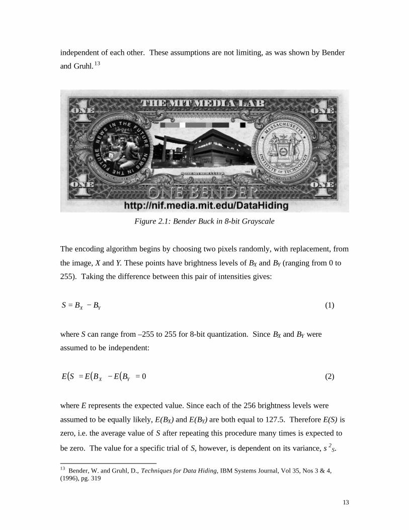
Buck”12 shown in Figure 2.1. Each pixel of such an image exists as a number in the

image file, where the number, in this discussion, is an integer that ranges from 0 to 255.

The number defines the intensity of that pixel, higher numbers being brighter. The

amount of quantization therefore defines how many different brightness levels are

available for the image. A simplifying assumption that will be made for the following

analysis is that all brightness levels are equally likely and that all samples are

11 Sweene, P., Error Control Coding (An Introduction), Prentice-Hall International Ltd., Englewood Cliffs,NJ, (1991)12 Fabricated Media Laboratory Currency created by Fernando Paiz

13

independent of each other. These assumptions are not limiting, as was shown by Bender

and Gruhl.13

Figure 2.1: Bender Buck in 8-bit Grayscale

The encoding algorithm begins by choosing two pixels randomly, with replacement, from

the image, X and Y. These points have brightness levels of BX and BY (ranging from 0 to

255). Taking the difference between this pair of intensities gives:

YX BBS −= (1)

where S can range from –255 to 255 for 8-bit quantization. Since BX and BY were

assumed to be independent:

( ) ( ) ( ) 0=−= YX BEBESE (2)

where E represents the expected value. Since each of the 256 brightness levels were

assumed to be equally likely, E(BX) and E(BY) are both equal to 127.5. Therefore E(S) is

zero, i.e. the average value of S after repeating this procedure many times is expected to

be zero. The value for a specific trial of S, however, is dependent on its variance, σ2S.

13 Bender, W. and Gruhl, D., Techniques for Data Hiding, IBM Systems Journal, Vol 35, Nos 3 & 4,(1996), pg. 319

14

How tightly the distributions of the individual values of S will cluster around E(S)

depends on σ2S. Because BX and BY were assumed to be independent, the following can

be said:14

222YX BBS σσσ += (3)

Assuming a uniform distribution of brightness, the variance of a particular pixel can be

calculated by:

( )75.5418

120255 2

2 =−

=XBσ (4)

Since both pixel X and Y are chosen randomly from the same data set, selected with

replacement:

22YX BB σσ = (5)

5.1083775.541875.5418222 =+=+=YX BBS σσσ (6)

1045.10837 ≈=Sσ (7)

where σS is the standard deviation of S. Nothing very useful can be said of a particular

value of S.15 However, if a statistic Sn is constructed from numerous iterations of S:

( )∑∑==

−==n

iYX

n

niin ii

BBSS1

(8)

14 Drake, A. V., Fundamentals of Applied Probability , McGraw-Hill, Inc., New York, NY, (1967), pg. 5615 Bender, W. and Gruhl, D., Techniques for Data Hiding, IBM Systems Journal, Vol 35, Nos 3 & 4,(1996), pg. 317

15

where n is the number of pairs of pixels taken. On average, as n approaches infinity, it

can be expected that nSn will approach zero. From independence, it is seen that the

expected value of Sn :

( ) ( ) 00 =×=×= nSEnSE n (9)

This result can be rationalized intuitively. Since pairs of points are chosen with

replacement, and at random, one would expect that pixel X will be brighter than pixel Y

about as many times that the reverse is true.

The variance of Sn can provide revealing information regarding the trend in S over many

trials. This is crucial to the development of the Patchwork algorithm.

From independence and zero mean it can be seen that:

22SS n

nσσ ×= (10)

104×≈×= nn SSnσσ (11)

With this formula, it is now possible to calculate the variance of Sn for a given number of

iterations. It was arrived at through experimentation that an appropriate value of n for

encoding a 1198x508 pixel image (e.g. one that would result from a 135dpi grayscale

scan of a Bender Buck, as seen in Figure 2.1) is 10,000:

400,10104000,10000,10

=×≈Sσ (12)

By the Central Limit Theorem, S10,000 can be approximated as a Gaussian with a mean of

zero, and a variance 000,10Sσ .16 Figure 2.2 shows the expected S10,000 distribution for a

Bender Buck. The Patchwork encoding method acts to shift this distribution through

16

modifications discussed in the next section. This shift in Sn when an image is encoded is

essentially what the Patchwork decoder (Section 2.5) uses to detect a watermark.

Figure 2.2: Expected S10,000 Distribution for a Bender Buck, 400,10000,10

=Sσ

2.3 Encoding MechanismIn Patchwork, the first task for encoding an image is the generation of a set of points to

alter in the image. These alterations are the physical manifestation of the digital

watermark and cause the encoded distribution of Sn to be shifted away from unencoded

distribution of Sn. These alterations take the form of changes in brightness. In order for

the decoder to recognize the watermark, it is crucial that it visit the same set of points in

the image. If this does not occur, or if only some of these points are revisited, non-

encoded points will be analyzed and the experimental value of Sn obtained from an

encoded distribution will not be shifted as far as intended. Depending on how far this

value of Sn ends up being shifted relative to the unencoded distribution in Figure 2.2, this

may result in loss of data or at least a decrease in decode certainty. This is discussed

further in Section 2.4. The ability to revisit the same points is therefore very important.

To generate a reproducible set of points, a pseudo-random number generator was used.

Such a number generator requires a key, or a seed, in order to return a number.

Successive use of the generator with the same seed results in a stream of pseudo-random

numbers between 0 and 1. When two such pseudo-random numbers are taken and scaled

16 Drake, A. V., Fundamentals of Applied Probability , McGraw-Hill, Inc., New York, NY, (1967), pg. 215

-100000 -80000 -60000 -40000 -20000 0 20000 40000 60000 80000 100000

17

to the dimensions of the image, the position of a pixel can be obtained. In this way, the

pixel positions that are needed in the algorithm can be generated pseudo-randomly. The

important factor, however, is that when the pseudo-random number generator is supplied

with the same seed later, e.g. during decode, the same stream of numbers is regenerated.

A unique set of numbers can therefore be generated with a particular key and it is only

necessary to know which key was used during encoding. Various encryption methods

can be used to make this key secure in practical use if the need arises, such as RSA or

PGP. When the same seed is used in conjunction with proper image alignment

(discussed in Chapter 4 and 5), the watermark can be detected by the decoder.

The encoding then starts by obtaining a point (X,Y), returned by scaling a pair of pseudo-

random numbers by the dimensions of the image. In order to modify the image so that

the encoded distribution of Sn can be separated from the unencoded distribution, the

brightness at point X is raised by δ while the brightness at point Y is lowered by the same

amount (it is not necessary that the second point be lowered by the same amount, only

that it be lowered). For simplicity, δ is used for both X and Y.

( )( )∑=

−−+=n

ibiain BBS

1

' () δδ (13)

( )∑=

−+=n

ibiain BBnS

1

' 2δ (14)

where S’n is the experimental value of Sn for an encoded image. In this way, each

additional pair of pixels add 2δ to the accumulating sum. Therefore, after n repetitions:

nSE n δ2)( ' = (15)

where the standard deviation is the same as in the unaltered distribution. From this

analysis, it can be seen that as n or δ increases, the distribution of Sn shifts in the positive

direction. As discussed in Section 2.4, shifting the S’n distribution far enough in this

direction makes any particular point that falls under one distribution highly unlikely to be

18

near the mean of the other. Therefore, an encoding can be successfully distinguished

from noise by looking at the value of Sn for that specific key. If it is sufficiently large in

magnitude, where large depends on the certainty level that is desired, it can be said with

confidence that encoding exists under that key. The level of certainty depends on the

distance of Sn from zero with respect to nSσ . A higher level of certainty requires that

E(S’n) be further (more standard deviations) from zero. An encoded image can then be

distinguished from a non-encoded image using a Hypothesis Test (Section 2.4).17

Once the image has been encoded, it is saved and written to file. The resulting grayscale

encoded image is then merged with its color components to produce the final encoded

image, as seen in Figure 2.3a. The original color image is seen in Figure 2.3b. As

expected, these images should appear identical. Extending the above algorithm for

multiple-bit encoding is presented in Chapter 6. The C program, encode.c, which was

written to perform the encoding procedure appears in Appendix A.

Figure 2.3a: Encoded Bender Buck

17 Drake, A. V., Fundamentals of Applied Probability , McGraw-Hill, Inc., New York, NY, (1967), pg. 240

19

Figure 2.3b: Original Unencoded Bender Buck

2.4 Hypothesis TestingHypothesis testing involves the use of a threshold to make a decision as to whether a

situation is true. In this case, the hypothesis being tested is whether the image in question

is encoded. Figure 2.4 plots both the encoded and non-encoded distributions on the same

axis. As discussed earlier, Patchwork serves to shift Sn to the right, thus separating the

encoded distribution from that of the unencoded (where the shift is dependent on δ and

n). A threshold is assigned so that an experimental value of Sn greater than the threshold

implies that the image is encoded. One possible threshold is shown in Figure 2.4. This

threshold lies three standard deviations from 0 (the mean Sn of the non-encoded image).

Since Sn is approximated to be Gaussian, there is a 0.13% chance that an experimental

value of Sn from a non-encoded image would occur at this value.18 As the threshold

moves further to the right this percentage decreases. At the same time, the likelihood of

that experimental value being obtained from an encoded image increases as the threshold

moves closer the mean of S’n. Therefore, an image that yields an experimental value of Sn

= z that falls in a region that is sufficiently far from 0 (as seen in Figure 2.4) can be

declared with certainty (depending on how far z is from 0) to not be from an unencoded

image. The further z is from 0, the less likely that such a value came from an unencoded

18 ibid. pg. 211

20

image. As mentioned before, if z was found to be 3000,10Sσ , there is only a 0.13% chance

that the image was non-encoded.

Figure 2.4: Hypothesis Test for an Image when Sn > Threshold

Figure 2.5:Hypothesis Test for an Image when Sn < Threshold

Figure 2.5 shows the case where the experimental value of Sn=z is less than the threshold

because the same points were not visited. In this case the data would could not be

recovered with the same level of certainty as before because it is not as far from the

unencoded distribution. As established earlier, it is important for the decoder to revisit

-100000 -50000 0 50000 100000 150000 200000

Encoded

Unencoded

z

-100000 -50000 0 50000 100000 150000 200000

Encoded

Unencoded

z

Threshold

Threshold

21

the same points. This is the basic premise upon which the Patchwork encoding/decoding

algorithm pair was created.

2.5 Decoding MechanismIn order to decode the image, the correct seed is needed to generate the correct pixel pairs

for analysis. This set of points and their position with respect to a set of axes will be

called the decode window. This decode window is visualized in Figure 2.6 where two

pixel pairs were decoded. Figure 2.6a shows the points where the image was encoded.

Figure 2.6b shows the decode window. In order to decode the image, the decode window

must coincide with these points precisely. Figure 2.6c shows the case where this window

does not coincide. In this case, the image cannot be successfully decoded since the

encoded points are not “seen” due to a rotation in the decode window. The points in the

decode window are generated identically to the manner in which it was generated in the

encoder. Using the same key, the pseudo-random number generator returns the same set

of points for the decoder to visit.

Figure 2.6a: Encoded Bender Buck with Points of Encoding Visualized

The decode window revisits the points and calculates Sn for that key and window. As

mentioned above, using a hypothesis test on the value of Sn, a degree of certainty can be

associated with whether the image was encoded or not. For example, if Sn for the case

where n=10,000 was found to be 93,600, one would conclude with great certainty (nine

22

standard deviations) that the image in question was encoded. The C program, decode.c,

which was written to perform the decoding procedure appears in Appendix B.

Figure 2.6b: The Decode Window for Figure 2.6a with Decoding Points Visualized

Figure 2.6c: Decode Window Misaligned Due to Rotation

Figure 2.7 shows the result when the Bender Buck in Figure 2.1 was encoded with

n=10,000 and δ=10 by seeding the pseudo-random number generator with the number

10. Figure 2.8 shows the Sn values when this encoded image was decoded with seeds 0

23

through 20 under perfect alignment of the decode window. Since each key generates a

unique set of points, only when the decoder is seeded with the same key that was used

during encode will the decoder visit the same points. Therefore, it is expected that only

key 10 will detect the encoding. It is clear from Figure 2.8 that the value of Sn for key 10

is much larger than the other values that form a baseline around zero. For key 10,

Sn=201,541. This is more than eight standard deviations (000,10Sσ = 10,400) from zero.

Therefore, it can be said with a very high degree of certainty that encoding exists in this

image at key 10.

Figure 2.7: A Bender Buck Encoded with n=10,000 and δ=10

Figure 2.8: Sn Values Obtained From Decoding Figure 2.7

-5.E+04

0.E+00

5.E+04

1.E+05

2.E+05

2.E+05

3.E+05

0 2 4 6 8 10 12 14 16 18 20Pseudo-Random Number Generator Key

Dec

ode

Sum

(Sn)

24

This is the basic mathematical model of the Patchwork encoding/decoding algorithm. It

allows for the fulfillment of the six restrictions and features presented in Section 2.1. As

has already been discussed, the Patchwork algorithm encodes watermarks into the media

itself, rather than into a header. In this way the data can remain within the image across

file formats and media. Also, the visibility of the encoding, as demonstrated by Figure

2.3, is very low. Using other modifications, such as a visibility mask (discussed in

Section 3.7), will further decrease the appearance of the data. Using the gradient descent

techniques discussed in Chapter 5 will extend Patchwork so that the decoder can recover

alignment and thus recover data when only a fragment of the host is available. In

addition, error correction coding will be incorporated into the Patch Track encoder and

decoder to ensure data integrity in the presence of noise. Patchwork can be made more

robust to several anticipated manipulations such as noise, cropping and lossy

compression with the additions discussed in the next section.

25

Chapter 3:

Encoding Algorithm Parameters

3.1 BrightnessThe choice of brightness as the method of encoding, rather than some other variable in

the image, was due in large part to the fact that the human visual system (HVS) has high

sensitivity to random changes in luminance, or brightness.19 By utilizing brightness, this

algorithm hides the data in regions of the picture that compression and reproduction

(changing formats, printing, etc.) techniques put the most effort into preserving. This

increases the likelihood that the mark is retained through format and media changes.

While the brightness level of certain pixels is actually being changed in the image, these

alterations are imperceivable to the human eye. The exact change in brightness (δ) that is

applied to the image is dependent on the image itself and the desired encoding “strength”.

Since the degree of certainty that is associated with an experimental value of Sn depends

on its value, a stronger encoding, or higher degree of certainty, can be achieved by

increasing δ, thus increasing S’n (Equation 13). Increasing δ will generally also have the

effect of making the encoding more obvious. In this way, a balance must be struck

between increasing certainty and decreasing perceivability. This tradeoff between

visibility of encoding and encoding strength arises many times in the use of this

algorithm.

To demonstrate this tradeoff, the Bender Buck is encoded with δ=80 and n=10,000 in

Figure 3.1. The corresponding S’10,000 for this image was found to be 1,303,090.

Comparing Figure 3.1 to Figure 2.7 (δ=10, n=10,000, S’10,000=201,541 ) shows that while

26

the image with δ=80 is more visibly encoded, its S’10,000 value is also much higher,

meaning the data can be decoded with more confidence. In fact the same effect can be

achieved by increasing n instead, as will be seen later.

Figure 3.1: Bender Buck Encoded with n=10,000 and δ=80

3.2 Patch Encoding

In the development of the Patchwork encoding algorithm in Chapter 2, the watermark

existed as points in the image. An improvement to this method uses patches, small

regions in the image rather than individual points. This modification offers two specific

advantages. One is the increased robustness of this encoding. Using patches decreases

the spatial frequency of the noise introduced by this algorithm, thus making the encoding

more resistance to lossy compression (such as JPEG compression) and finite input

response filters. Patches make the encoding appear less like noise, as single points

would, and more like important parts of the image in the eyes of the JPEG compressor.

This helps to keep the encoding from being removed from the image during conversion to

JPEG. In addition, patches help facilitate the decoding of the image under practical

circumstances. By placing the encoding in a region larger than an individual point (or

“chip”), while keeping the decoding mechanism the same, a more a forgiving alignment

is required when attempting to detect the watermark in the image.

19 Lim, Jae, Two Dimensional Signal and Image Processing, Prentice-Hall Inc.,Englewood Cliffs, NJ(1989), pg. 429-37

27

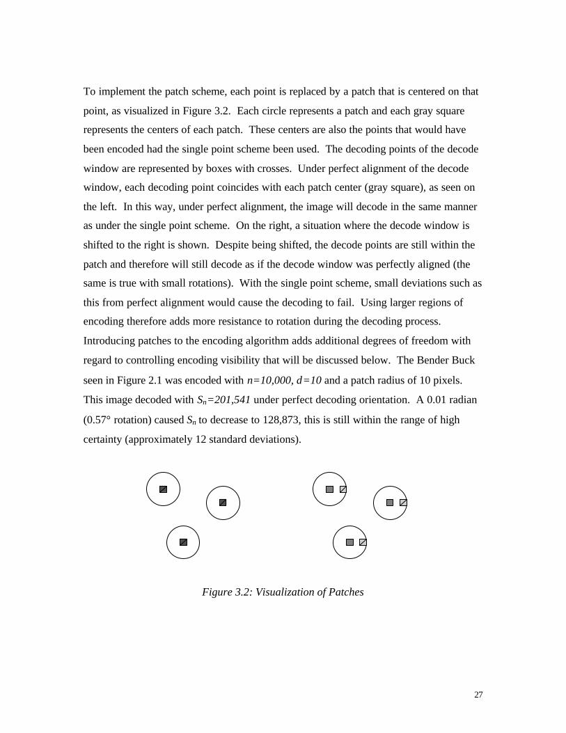
To implement the patch scheme, each point is replaced by a patch that is centered on that

point, as visualized in Figure 3.2. Each circle represents a patch and each gray square

represents the centers of each patch. These centers are also the points that would have

been encoded had the single point scheme been used. The decoding points of the decode

window are represented by boxes with crosses. Under perfect alignment of the decode

window, each decoding point coincides with each patch center (gray square), as seen on

the left. In this way, under perfect alignment, the image will decode in the same manner

as under the single point scheme. On the right, a situation where the decode window is

shifted to the right is shown. Despite being shifted, the decode points are still within the

patch and therefore will still decode as if the decode window was perfectly aligned (the

same is true with small rotations). With the single point scheme, small deviations such as

this from perfect alignment would cause the decoding to fail. Using larger regions of

encoding therefore adds more resistance to rotation during the decoding process.

Introducing patches to the encoding algorithm adds additional degrees of freedom with

regard to controlling encoding visibility that will be discussed below. The Bender Buck

seen in Figure 2.1 was encoded with n=10,000, δ=10 and a patch radius of 10 pixels.

This image decoded with Sn=201,541 under perfect decoding orientation. A 0.01 radian

(0.57° rotation) caused Sn to decrease to 128,873, this is still within the range of high

certainty (approximately 12 standard deviations).

Figure 3.2: Visualization of Patches

28

3.3 Patch SizeThe size of the patches is an important parameter with distinct tradeoffs. Increasing the

size of the patch can allow for easier alignment of the image in the decode stage. From

Figure 3.2, it can be seen that a larger patch will resist more shift and rotation in the

decode stage. Increasing the patch size will also cause patches to overlap sooner with

respect to increasing patch number. In effect, patches in the encoding will begin to

interfere with other patches sooner. It will be seen later in Chapter 4 and 5 that resistance

against rotation and shift becomes less important with the addition of a gradient descent

to the decoding system. For the example visited in the previous section, doubling the

patch size increases the 0.01 radian rotation S’n to 154,596.

3.4 Patch ShapeAnother parameter to consider is the shape of the patches. This parameter in particular

has an important impact on the visibility of the encoding. The HVS is particularly

sensitive to regular or lattice-like placement (patterns) of objects with continuous edges.20

These patterned edges contain high frequencies, a feature that was described earlier as

being particularly apparent to the HVS. In order to take advantage of this characteristic,

the choice of circular patches was made. In addition, since patches are placed randomly

in the image by this algorithm, lattice-like formations are avoided.

3.5 Number of Patches

Similar to the choice of δ, the number patches, n, also impacts the encoding strength.

From Equation 13, it can be seen that increasing n will also increase S’n. Again, having a

higher value of S’n, means a higher certainty of encoding. However, as was mentioned

with increased patch size, increasing the number of patches also tends to decrease the

space for other patches. Too many encodings also has the effect of degrading the image

as seen in Figure 3.3 where the Bender Buck is encoded with n=15,000, δ=20 and radius

of 10. A recommended n for a typical 1198x508 pixel image was found to be 10,000.

20 Bender, W. and Gruhl, D., Information Hiding to Foil the Casual Counterfeiter, (1998), pg. 7

29

Figure 3.3: A Bender Buck Encoded with n=15,000, δ=20 and radius of 10

3.6 Patch Intensity and ContourAs mentioned above, the HVS appears to very sensitive to low frequency patterns 21. To

take advantage of this characteristic, a good patch choice would be blob shaped, but one

that did not have a constant intensity throughout its area. Instead, if the area was filled

with pseudo-random intensity values, the patches would appear less patterned, and thus,

less visible. Such a randomly filled circle is visualized in Figure 3.4. While this

modification would make the patches less visible, it would have a deleterious affect on

the encoding. A given patch may or may not have the desired δ change in brightness

anymore at the point of decode. This would serve to undermine the basis of the encoding

algorithm.

Figure 3.4: Side View of a Pseudo-Randomly Filled Circle

A compromise can be achieved by using a “contour” that shapes the random intensities in

the patch. Figure 3.5 visualizes a negative patch that has contoured random intensities.

Here it can be seen that while a large degree of randomness is retained in the contoured

21 ibid.

30

image, encoding coherency is also maintained by applying an envelope to the random

intensities. A perfectly aligned image will decode at the center of the patch, the apex or

nadir of the contour, matching the result associated with a constant patch. This contour

thus maintains the benefits of patch usage, such as rotation and shift resistance, while

reducing visibility. Due to the shape of the contour, we refer to this type of patch as a

“random cone.” Because humans tend to notice sharp edges and continuous patterns

more readily than gradients and randomness, a patch contour that takes advantage of this

fact will allow for “stronger” encoding while remaining well hidden. Since the random

cone does not lend itself towards sharp edges, due to its contouring, nor patterns, because

it is circular and placed randomly, random cones are an advantageous choice of patch

type.

Figure 3.5: Side View of a Negative Random Cone22

3.7 Visibility MaskAn additional refinement to the encoding algorithm involves the use of something that

will be referred to as a visibility mask. By identifying regions in an image that are most

suitable for encoding (regions in which the patches will be least noticeable) it is possible

to conceal data in an image. Such regions are those that exhibit a large amount of high

frequency content. Applying changes to regions of an image that contain a great deal of

variation in brightness is less detectable to the HVS than applying the same changes to a

region that varies less23. Adding a patch to a region of an image that is high frequency

22 ibid.23 ibid.

31

(contains drastic changes in intensity) is much less visible than adding the same patch to

a region of an image dominated by low frequencies. The visibility mask seeks to identify

the high frequency regions in the target image and concentrate the encoding there.

The visibility mask was implemented using a double sinc blur technique diagramed in

Figure 3.6. The image resulting from the first blur, which takes the average value of the

points in a square window and replaces the center of that square with the average, was

subtracted from the original image, resulting in a difference image. Since the blurring

process attenuates high frequencies from the image, this difference image then contains a

rough estimate of all the edges in the image (absolute value of high frequency areas). A

second blurring, increases the width of these edges. In this way, high frequency regions

in the image were identified for visibility masking of the encoding. The appropriate size

of the blurring kernels depends on the size of the image. It was found that for 1198x508

pixel image, a good set of blur kernel sizes was 5x5 for the first blur and 7x7 for the

second blur.

Figure 3.6: Block Diagram of the Double Sinc Blur Technique

This double blur process was added to the encoding algorithm after the patch locations

were identified. Before applying these patches, however, the visibility mask was

implemented by scaling the brightness change (δ) by a factor that measures the

desirability of that location in terms of its frequency content. For example, if this

position fell on a sharp edge, as specified by the visibility mask, a scale factor near 1 is

used. If this position fell in a constant region, a scale factor near 0 is used. Intermediate

cases were then assigned a scale factor relative to how much high frequency content was

Sinc Blur

+

_

Sinc BlurTarget Image

32

present in that area. In this way, very blatant encodings can be avoided while decresing

the perceivability of the data.

These are the many elements of the basic Patchwork algorithm. Each aids in adding the

desired robustness and/or decreased visibility as discussed in Chapter 2. In practice these

elements of the encoding algorithm perform well. In order to encode with multiple bits,

however, a further modification to the decoding process is necessary. This is the

inclusion of an orientation detector, allowing for more resistance to rotation.

33

Chapter 4:

Orientation Detection and Correction

4.1 MotivationThe robust nature of the Patchwork algorithm allows watermarked images to be printed

while retaining the embedded information. In order to retreive this data, it is necessary to

scan the paper image into digital format. A practical issue that must be addressed in this

context is that of image alignment during the decoding process. The orientation of an

image on a flatbed scanner is inherently imprecise. When using a desktop scanner, the

mere act of closing the cover can drastically change the position of the image from where

it was placed. Therefore, it is neither sufficient nor practical to require the user to

accurately position the picture on the scanner in the correct orientation. One possible

solution to this alignment problem is the use of an orientation detection and correction

mechanism. By integrating such a mechanism into the decoder, an image can be placed

on the scanner in an arbitrary orientation. The decoder would then determine the

orientation and extract the data, thus maintaining the ability to decode the image.

The addition of orientation detection and correction also allows for a hierarchical

approach to the decoding of a target image embedded by Patch Track (multiple bits).

One appropriate use of digital watermarkering, as mentioned earlier, is the encoding of

images with reference numbers, perhaps indicating ownership by a particular company.

In order to place such a watermark, as will be discussed further in Chapter 6, multiple bits

will be required. Until this point, only the single bit case has been discussed. Multiple

bits can be implemented as a sequence of positive and negative Sn values that represent

ones and zeros using Patch Track (discussed in Section 6.1). Since the encoding

34

algorithm embeds watermarks for different keys in a nearly orthogonal manner24 (due to

the pseudo-random number generator), many bits can usually be encoded in an image

before either degrading the image or interfering the encoding of other bits. For a Bender

Buck, approximately 256 bits can be encoded before significant image degradation

occurs.

In Patch Track, the first bit in the sequence of bits that constitute the multiple-bit

encoding can serve as an encoding identifier, one that indicates if the image has been

encoded at all. Thus, a hierarchy is created in the decoding process. First, it is

determined whether encoding exists in the image. Then, given that a watermark is

present in this image, the remainder of the watermark is read by the decoder.

This hierarchy is extremely useful in multiple bit encoding. When it is possible, it is

certainly desirable to decrease δ or n while maintaining the strength of encoding. Doing

so would lower the visibility of the encoding. However, decreasing either δ or n will

have a direct effect on Sn. The Patch Track hierarchy, however, provides an alternate

solution. A lighter encoding of the majority of the information is possible if the strong

encoding of the first bit is used to signify the presence of data. In this way, the first bit of

the stream of data bits is used to identify whether data is present in the image. If all of

the information bits are encoded lightly, e.g. the 75% certainty level, there will be one

failure in every four bits decoded. For some applications, this is not sufficient. For

example, a much higher degree of certainty, perhaps 99.999% may needed when tracing

images on the Internet.25 Otherwise, because of the magnitude of images on the Internet,

the process of tracking the encoded image will be overwhelmed by false alarms.

Encoding all of the data at the 99.999% certainty level may cause the data to become

obvious in the image. If only the first bit is encoded at this strength, it can be known with

99.999% certainty that there is encoding in this image. Far less encoding is then required

for the remaining bits of the watermark since it only needs to be determined whether

these bits are positive or negative. Error correction coding can then be used to increase

24 ibid. pg. 925 ibid. pg. 11

35

the fidelity of these data points, as discussed in Chapter 5. This reduction in encoding

power helps retain image quality while maintaining the accuracy of data recovery. It is

therefore helpful to have a mechanism that aligns the image quickly and prepares it for

decoding. Once this is done, the presence of the strong bit can be determined.

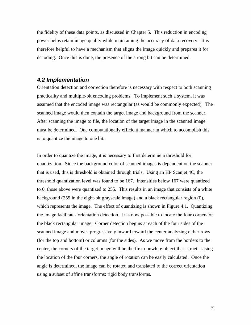
4.2 ImplementationOrientation detection and correction therefore is necessary with respect to both scanning

practicality and multiple-bit encoding problems. To implement such a system, it was

assumed that the encoded image was rectangular (as would be commonly expected). The

scanned image would then contain the target image and background from the scanner.

After scanning the image to file, the location of the target image in the scanned image

must be determined. One computationally efficient manner in which to accomplish this

is to quantize the image to one bit.

In order to quantize the image, it is necessary to first determine a threshold for

quantization. Since the background color of scanned images is dependent on the scanner

that is used, this is threshold is obtained through trials. Using an HP Scanjet 4C, the

threshold quantization level was found to be 167. Intensities below 167 were quantized

to 0, those above were quantized to 255. This results in an image that consists of a white

background (255 in the eight-bit grayscale image) and a black rectangular region (0),

which represents the image. The effect of quantizing is shown in Figure 4.1. Quantizing

the image facilitates orientation detection. It is now possible to locate the four corners of

the black rectangular image. Corner detection begins at each of the four sides of the

scanned image and moves progressively inward toward the center analyzing either rows

(for the top and bottom) or columns (for the sides). As we move from the borders to the

center, the corners of the target image will be the first nonwhite object that is met. Using

the location of the four corners, the angle of rotation can be easily calculated. Once the

angle is determined, the image can be rotated and translated to the correct orientation

using a subset of affine transforms: rigid body transforms.

36

Figure 4.1: One-Bit Quantized Image Using a Brightness Threshold of 167

Rigid body transforms allow for two dimensional translation and rotation. To apply a

horizontal shift of m, a vertical shift of n and a rotation of θ to a point (x,y) the following

equation is used:

37

=

−

1'

'

1100cossin

sincos

y

x

y

x

n

m

θθ

θθ

(16)

which can be decomposed to:

=

−

1'

'

11000cossin

0sincos

10010

01

y

x

y

x

n

m

θθ

θθ

(17)

where the first matrix is applies a translation and the second matrix applies a rotation to

point (x,y). The resulting point (x’,y’) is the shifted, rotated version of (x,y).

The actual implementation of this transform is in the inverse direction. The points that

are obtained from the scanned image form the set of (x’,y’) and the goal is to obtain the

original position of these points, (x,y). Therefore, the following inverse affine transform

is applied to the points in the scanned image:

=

−−−

11''

1001001

1000cossin0sincos

11

yx

yx

nm

θθθθ

(18)

In this way it is possible to obtain the original orientation of the image. To rotate and/or

shift an image, this transformation is applied to all pixels in the image. Any rotation or

shift that is detected by this algorithm can therefore be corrected with this inverse

transformation. Using the dimensions obtained from the corner identification the image

is cropped and written to file for decoding.

This method of orientation correction is useful when one requires a fast, yet accurate

determination of whether a watermark exists in an image and when the image has been

encoded in the normal viewing orientation. Since it depends only on the fact that the

38

image is rectangular (and fit on the scanner), this is the only requirement of the

algorithm. In more general cases, including the decoding of randomly oriented encoding,

data recovery from partial or cropped images and decoding the rest of the information in

multiple-bit encoding, a more computationally intensive approach is required, and is

described in the next chapter. Since this is a very rough estimation of the correct

orientation of the image, as can be seen from the noise present in the quantization (Figure

4.1), a fairly large chip is required for data to be extracted. Through experimentation, it

was found that a good patch size is 15 pixels at 135dpi. The C program, odetect.c, which

was written to execute the above orientation correction appears in Appendix C.

This orientation detection and correction system, as stated earlier, can be used simply to

aid the alignment of scanned images or as a part of the multiple-bit decoding scheme. In

the latter, this system would account for the first stage of orientation correction, the rough

alignment. It is then followed by a random search in the proximity of the roughly aligned

image and a final adjustment of alignment by a gradient descent.

39

Chapter 5:

Improved Decoding by Random Search/GradientDescent

5.1 MotivationIt has been assumed thus far that the image in question has been encoded in the expected

manner, that is, in the normal viewing orientation. Certainly an image can easily be

decoded at an arbitrary orientation, thus leaving the approach described in Chapter 4 less

than useful. While the image may be aligned correctly visually, it will not be in the

correct orientation for decoding. In addition, cropping of the image may have occurred,

in which case, the shape of the target image may no longer be the same. Suppose only

part of the image was available for decoding or part of the image was obscured. It would

be desirable to have a mechanism that could handle these cases. One possible

implementation is the use of a gradient descent, described below. Using this search

method allows for orientation correction regardless of image shape and encoding

orientation but at much higher cost in terms of decoding time.

5.2 Gradient DescentConsider the representation of a negative patch in Figure 3.5. As described in Section

3.6, this is a side view of a non-random cone (a non-random cone is used here for clarity,

the situation applies for a random cone also, as will be discussed below). The objective

of the decoding algorithm is to have all of the decoding points (Xi and Yi from Equation

3) correspond to the apex of the cone. This is perfect decoding alignment because it

results in the largest possible decode value (in the correct alignment, when seeded with

the same key, the decoder will pick the same points as the encoder). Under perfect

alignment, |Sn| is maximized, as seen in Figure 5.1 where the gray dot indicates the

decode point. If, however, the orientation is not correct, a situation such as the one seen

40

in Figure 5.2 might occur. Here the decoding window is shifted to the left by six pixels

(the same argument holds for rotation). When the decoding window is not correctly

oriented, the decoding is much less successful since the full δ is not detected in all

patches. In the patch seen in Figure 5.2, the situation is particularly bad since the

decoding point falls on a value that has been nearly unaltered from the background

brightness level. Depending on the original orientation, other decoding points may not

even land in a patch, resulting in a significantly smaller Sn. This can obviously hinder the

ability to recover the desired data. Orientation is therefore crucial.

Figure 5.1: Perfect Decode Window Orientation

Figure 5.2: Imperfect Decode Window Orientation

In order to properly orient the decoding points, it is possible to follow the gradient of the

cone (in gray images) toward the nadir. This is the essence of a gradient descent. To

accomplish this, the gradient of brightness at the current, imperfect, decoding point is

calculated and used to determine which the decode window should move. The gradient is

41

determined by calculating Sn for the current window orientation as well as for all three

possible degrees of freedom: horizontal shift, vertical shift and rotation. From these four

Sn calculations, the largest slope magnitude is identified. The window is then moved in

the corresponding direction (depending on the sign of the slope) and the gradient analysis

is performed again. This is then done repeatedly until the apex is reached. At this point,

the gradient should be zero. In Figure 5.2, the window would initially move to the right.

The amount that the window should move after each iteration of the gradient descent, or

schedule size, is a complex topic and depends on various factors such as image size.

Through trial and error, it was found that a good fixed schedule was a step size was 2

pixels and a rotation of 0.5°.

Figure 5.3:Misleading Points Used in Calculating the Gradient

The use of a gradient descent in the case of random cones is slightly more involved.

Since the random cones possess random intensities the straightforward gradient analysis

is not sufficient. The random intensities that were inserted to decrease data visibility

unfortunately add too much noise to the system for a simple slope calculation as might be

performed in the non-random case. Calculating the slope of the surrounding points (gray)

in a random cone can be misleading, as seen in Figure 5.3, where the slope calculated

from the gray point indicates the wrong direction of traversal. To circumvent this

problem, minimum absolute deviation regression analysis was used.26 Rather than

calculating the gradient of the intensities, a best-fit lines is calculated using the Sn values

that would result from moving ten points in the positive direction and ten points in the

42

negative direction from the current decoding point, in the two possible translation

directions. Rotation is treated similarly with steps in degrees. The slopes of these best-fit

lines are then used to determine the direction of window movement. In this way, the

contribution from noise introduced by the random intensities is reduced well enough to

reveal the underlying gradient. The decode window is then moved, as in the non-random

case, in the direction indicated. This process is repeated until the nadir is reached.

5.3 Advantages and Implementation of Random Search andGradient DescentThe gradient descent described above is implemented with regard to multiple-bit

encoding by locating the orientation that maximizes the Sn of the strong marker bit. Since

the shape of the scanned image is not utilized in the orientation detection, this method

provides a way to orient a variety of differently shaped images (e.g. a rectangular image

that was cut in half in a jagged manner). The one requirement of the gradient search,

however, is the dimensions of the original image when it was encoded. These

dimensions are used to create the appropriate decoding window. Having such

information is well within reasonable expectations as the party (or parties with the rights

to the encoded information) that embedded the data would presumably be privy to this

information.

In this way, the orientation can be corrected for an image that has been partially lost,

intentionally disturbed or is just slightly different. With respect to the encoding, losing

part of the image only means that n, the number of encoded points, will decrease. This,

in turn, will decrease Sn but given a strong encoding, such a loss will not affect the ability

to decode the image. This is unlike the unoriented case where Sn is also decreased.

Under the unoriented case, the encoding is lost in the randomness of the cones. In the

partial image loss/perfect orientation case, the encoding is maintained, due to the

remaining available points that are aligned correctly. Since the number of encoding

points recovered is lower, Sn will be lower.

26 Press, W. H., Numerical Recipes in C , Cambridge University Press, New York, NY (1992), pg. 703

43

The alignment detection is implemented on two levels, one proximity random search

stage and one refinement stage. The scanned image will contain both the target image

and additional blank space from the remaining area on the scanner bed. Once this image

is acquired the orientation detection and correction described in Chapter 4 is performed.

This orientation correction provides a good estimate of the correct alignment of the

image. The random search stage consists of the acquisition of many Sn values

corresponding to a variable number of random orientations of the decode window. These

orientations are restricted to small displacements from the current orientation (produced

by the orientation detection and correction stage). Through experimentation it was found

that roughly 50 pixels of translation and 10 degrees of rotation perform well as limits to

these displacements. The number of random orientations that are tested is important to

the correct orientation detection. A sufficient number must be tested in order to generate

a decode window orientation that is sufficiently close to the actual encoding orientation

so that the gradient descent will work. Under testing conditions, this corresponds to an

orientation that decodes with Sn > 5σS and more than 6000 random orientations for a

1198x508 image. It required roughtly 15 minutes to complete this random search on a

Pentium II 450MHz PC with 512MB of RAM.

Given the size of the scanned image and the size of the original, a range for the shift

values is set and random values within this range are generated (angles must range from 0

to 2π). The image is decoded for the strong bit at each of these random orientations. A

variable set of the orientations corresponding to the highest Sn values is then cached and

saved for refinement in the second stage. Again, it is crucial to create a set of

orientations that are approximately correct at this stage. The refinement stage usually

does not incur more than a 1% change in the orientation of the image. For this reason, a

large number of orientations (>6000) should be used in the random search stage to insure

the proper result.

The refinement stage is precisely the gradient search algorithm that was discussed in

Section 5.2. When the image is correctly oriented, it is cropped and prepared for

decoding by the multiple-bit decoder described in Chapter 6. A Bender Buck that was

44

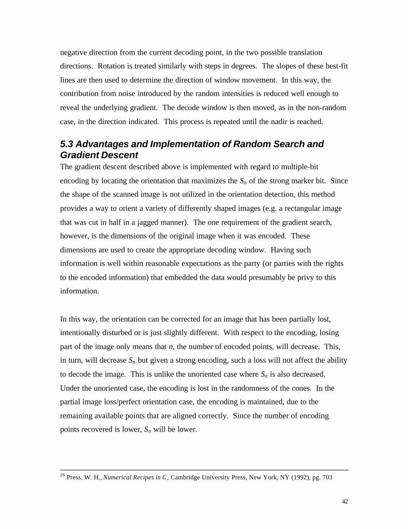
encoded with n=12,000, δ=40 and a random cone radius of 20. This image was then

printed out at 135dpi, cut and scanned back in at 135dpi, as shown in Figure 5.4. Using

the random search/gradient descent alignment correction method (using the top 10

decode windows from 10000 random orientations), it was possible to obtain the original

alignment as seen in Figure 5.5. This image was then cut and decoded with Sn=56,581.

The full image, when scanned in at an arbitrary orientation (Figure 5.6), decoded with

Sn=75,076. The lower decode sum for Figure 5.5 is due to the loss of part of the image.

Since the encoding exists in the pixels themselves, any loss of the image is accompanied

by a decrease in Sn. Nevertheless, both images were successfully decoded with high

degrees of confidence.

Figure 5.4: Scanned Image of the Cut, Encoded Bender Buck

The random search and gradient descent approach to the alignment problem yields good

alignment and high Sn values, but there are disadvantages. Perhaps the largest drawback

of this implementation is the time required to complete an alignment adjustment.

Because it uses a random search, it is computationally intensive. It requires roughtly 15

minutes to complete a random search for 6000 orientations and the gradient descent of

the ten best orientations on a Pentium II 450MHz PC with 512MB of RAM. This time

cost could hinder the use of this implementation in certain circumstances. Nevertheless,

images that are aligned with the random search and gradient descent method are done so

45

with good accuracy. It is believed that the random search and gradient descent algorithm

could be optimized from both a theoretical and programming perspective. One such

change would be an implementation in Perl rather than C, as was done in this research.

This could lower the time required to run this implementation to a few minutes.

Figure 5.5: Aligned Bender Buck Using Random Search and Gradient Descent

Figure 5.6: Full Bender Buck Before Random Search and Gradient Descent

Another problem that remains to be solved is that of image scaling during decode. The

current implementation of the gradient search does not consider the possibility of

46

receiving a scaled version of the original image. With horizontal and vertical translation

and rotation, this would increase the total number of degrees of freedom to four. By

increasing the dimensions of the search space, the algorithm would also require more

computation and more time requirements.

While this solution to the alignment problem is not optimal, it is sufficient to achieve

proper orientation of the image for decoding given that the image is rectangular and the

dimensions are known. Optimizing the search algorithm and implementing this

optimization in Perl is an appropriate continuation of this work. In addition, future

research could explore the problem of scaling presented above. The C implementation of

both the random search and gradient descent, grad.c, appears in Appendix D.

47

Chapter 6:

Multiple-Bit Encoding/Decoding

6.1 ImplementationThe multiple-bit encoder embeds a sequence of bits within an image in a specified order.

This sequence of bits can then be extracted by the decoder and used accordingly. The

decoder, for example, can convert the data into text. This is implemented, as discussed

earlier, by first encoding the strong bit with a specified key (zero). The data is then

encoded beginning at key one, with each successive key representing one bit. A one or a

zero is encoded with either a positive or negative Sn. This can be achieved by modifying

the basic encoding algorithm discussed in Chapter 2 with the ability to encode with both

positive and negative δ. This then allows the creation of a positive or negative Sn. After

orienting with the strong bit, it is only necessary to identify the sign of the following bits.

A positive Sn represents a 1 while a negative Sn represents a 0. The data is decoded in

this manner by stepping through all of the keys and determining the corresponding Sn.

The bits are then assigned according to whether the corresponding Sn is positive or

negative.

Error CorrectionAn additional feature that increases decoding accuracy while allowing a smaller δ to be

used is error correction coding. One possible scheme, used here, encodes the data in

triplicate. For example, if the data to be embedded is three bits long, keys 1, 2 and 3

would encode the first bit, keys 4, 5 and 6 would encode the second bit and keys 7, 8 and

9 would encode the third bit. This redundant coding allows for higher degrees of

certainty when all three of the bit encodings agree or error correction when one fails due

to noise. An example of this appears in Figure 6.1. Here the Bender Buck was

watermarked with four bits, “0,1,1,0” using the triplicate error correction scheme

48

discussed above. The C program, mbencode.c (Appendix E), was used to encode the

image with the strong bit encoded with n=10,000 and the data bits encoded with

n=2,000. All bits were encoded at δ=30 with a radius of 15. The image was printed out

and scanned back in at 135dpi. The random search and gradient descent alignment

correction functions were then run to adjust the image. Finally, the image was decoded

with the multiple-bit decoder implemented in C, mbdecode.c, seen in Appendix F. This

particular set of data did not utilize the error correction since each encoded bit was

extracted correctly.

Seed Decode Value (Sn)Strong Bit 39,8961 -3,4702 -3,1543 -13,7944 7,3225 2,5886 5,8947 9,7628 5,2529 7,07610 -7,95011 -11,27012 -8,568

Figure 6.1:”0,1,1,0” Sn Values Under Error Correction Scheme

For larger watermarks, each bit is encoded in this way until the desired data has been

wholly encoded. The amount of data that can be stored in a particular image depends on

the frequency content and size of the image. Typically this value ranges from 64 to 256

bits for most images.

The small amount of data that is contained in the image is not a significant limitation

given the availability of network access. Rather than trying to place all the information

that one would like to associate with a particular picture, a URL, filename or unique

49

serial number can be embedded instead, allowing for the dynamic updating information

rather than the continual re-encoding of the image with the most recent data.

50

Chapter 7:

Conclusion

A complete multiple-bit encoder/decoder pair was created from the Patchwork approach.

Beginning from the mathematical basis of the Patchwork algorithm for information

hiding in digital images, gradual improvements were developed that allowed for the

expansion to multiple-bit encoding (Patch Track) including: coarse orientation detection,

random search, gradient descent and multiple-bit encoding/decoding. These

improvements increased the usefulness of the Patchwork/Patch Track algorithm. Patch

Track is a valuable technique for watermarking digital images for its robustness and

allows the various watermarking applications discussed in Chapter 2.

Before the various uses for the Patch Track system can be successfully implemented,

however, some additional improvements are necessary. For example, the random search

and gradient descent is somewhat computationally intensive and does not currently

perform the alignment correction in a reasonable amount of time for most applications.

Solving this problem could be approached by optimization of the search algorithm and/or

the programming. This can be used in conjunction with the acquisition of additional

hardware. Unfortunately, an exhaustive search will always be one of the less efficient

methods for alignment correction. However, exhaustive searches are particularly well

suited for parallel computation. Increasing the number of CPUs involved in the random

search will decrease the time required. While a form of exhaustive search, the method

discussed in this thesis is nevertheless not a blind exhaustive search. Instead the process

is sped by gaining information incrementally, the aggregate of which takes less time than

a purely random search.

51

An additional problem that is left to be resolved is the extension of the decoder to account

for the possibility that the incoming image may be scaled from the original size. This

additional parameter will increase computing time and/or computation required.

This research has taken a significant step toward solving the alignment problem in digital

information hiding in images. By eliminating a purely exhaustive search, the time

required to properly align an image has been dramitcally reduced. In addition,

Patchwork/Patch Track has introduced various ways to decrease the visibility of

watermarks in images. Both of these improvements are provide an element of direction

to the development of more advanced watermarking techniques. It has been shown in

this research that the various advancements contained in Patchwork/Patch Track are

effective.

52

References

1. Anderson, R., Lecture Notes in Computer Science – Information Hiding, Springer,New York, NY, 1996.

2. Bender, W. and Gruhl, D., Techniques for Data Hiding, IBM Systems Journal, Vol35, Nos 3 & 4, 1996.

3. Bender, W. and Gruhl, D., Information Hiding to Foil the Casual Counterfeiter,Information Hiding, 1998.

4. Drake, A. V., Fundamentals of Applied Probability, McGraw-Hill, Inc., New York,NY, 1967.

5. Hardin, C. L., Color For Philosophers, Hackett Publishing Co., Indianapolis IN,1988.

6. Lim, J., Two Dimensional Signal and Image Processing, Prentice-Hall, Inc.,Englewood Cliffs, NJ, 1990.

7. Oppenheim, A. V. and Schaffer, R. W., Discrete-Time Signal Processing, Prentice-Hall, Inc., Englewood Cliffs, NJ, 1989.

8. Oppenheim, A. V. and Willsky, A. S., Signals and Systems, Prentice-Hall, EnglewoodCliffs, NJ, 1983.

9. Petitcolas, F., Attacks on Copyright Marking Systems, in Information Hiding, SecondInternational Workshop, IH'98, Portland, Oregon, USA, April 15-17, 1998, Springer-Verlag, New York, NY, pp. 219-239.

10. Petitcolas, F. and Anderson, R., Evaluation of Copyright Marking Systems. To bepresented at IEEE Multimedia Systems (ICMCS'99), 7-11 June 1999, Florence, Italy.

11. Press, W. H., Numerical Recipes in C, Cambridge University Press, New York, NY,1992.

12. Simon, M., Spread Spectrum Communications Handbook, McGraw Hill, Inc., NewYork, NY, 1994.

13. Skapura, D., Building Neural Networks, ACM Press, New York, NY, 1996.14. Sweene, P., Error Control Coding (An Introduction), Prentice-Hall International Ltd.,

Englewood Cliffs, NJ, 1991.15. DataHiding Homepage,

http://www.trl.ibm.co.jp/projects/s7730/Hiding/index_e.htm16. NECI Technical Report 95-10, http://www.neci.nj.nec.com/tr/neci-abstract-95-

10.html17. The information hiding homepage - digital watermarking & steganography,

http://www.cl.cam.ac.uk/~fapp2/steganography/