a robust estimation method of location and scale

A ROBUST ESTIMATION METHOD OF LOCATION AND SCALE WITH

APPLICATION IN MONITORING PROCESS VARIABILITY

ROHAYU BT MOHD SALLEH

A thesis submitted in fulfilment of the

requirements for the award of the degree of

Doctor of Philosophy (Mathematics)

Faculty of Science

Universiti Teknologi Malaysia

AUGUST 2013

v

ABSTRACT

This thesis consists of two parts; theoretical and application. The first part

proposes the development of a new method for robust estimation of location and

scale, in data concentration step (C-step), of the most widely used method known as

fast minimum covariance determinant (FMCD). This new method is as effective as

FMCD and minimum vector variance (MVV) but with lower computational

complexity. In FMCD, the optimality criterion of C-step is still quite cumbersome if

the number of variables p is large because of the computation of sample generalized

variance. This is the reason why MVV has been introduced. The computational

complexity of the C-step in FMCD is of order ( )3O p while MVV is ( )2O p . This is a

significant improvement especially for the case when p is large. In this case, although

MVV is faster than FMCD, it is still time consuming. Thus, this is the principal

motivation of this thesis, that is, to find another optimal criterion which is of far

higher computational efficiency. In this study, two other different optimal criteria

which will be able to reduce the running time of C-step is proposed. These criteria

are (i) the covariance matrix equality and (ii) index set equality. Both criteria do not

require any statistical computations, including the generalized variance in FMCD and

vector variance in MVV. Since only a logical test is needed, the computational

complexities of the C-step are of order ( ) ln O p p . The second part is the

application of the proposed criteria in robust Phase I operation of multivariate

process variability based on individual observations. Besides that, to construct a

more sensitive Phase II operation, both Wilks’ W statistic and Djauhari’s F statistic

are used. Both statistics have different distributions and is used to measure the effect

of an additional observation on covariance structure.

vi

ABSTRAK

Tesis ini mengandungi dua bahagian; teori dan aplikasi. Bahagian pertama

mencadangkan pembangunan kaedah baru untuk penganggaran teguh lokasi dan

skala, dalam langkah penumpuan data (C-langkah), dari kaedah yang paling

digunakan secara meluas dikenali sebagai penentu kovarians minimum cepat

(FMCD). Kaedah baru ini efektif seperti FMCD dan varians vektor minimum

(MVV) tetapi kerumitan pengiraannya adalah rendah. Dalam FMCD, secara

optimum kriteria bagi C-langkah masih agak rumit jika bilangan pembolehubah p

adalah besar disebabkan pengiraan sampel varians teritlak. Inilah alasan mengapa

MVV diperkenalkan. Kerumitan pengiraan C-langkah dalam FMCD adalah

peringkat ( )3O p manakala MVV adalah ( )2O p . Ini adalah satu peningkatan yang

bererti terutamanya untuk kes bila p besar. Dalam kes ini, walaupun MVV lebih

cepat daripada FMCD, pengiraannya masih mengambil masa. Oleh itu, motivasi

utama tesis ini ialah untuk mencari kriteria optimum yang lain dimana pengiraannya

jauh lebih efisien. Dalam kajian ini, dua kriteria optimum yang berbeza yang boleh

mengurangkan masa pengiraan di dalam C-langkah dicadangkan. Kriteria tersebut

adalah (i) kesaksamaan kovarians matrik dan (ii) kesaksamaan set indeks. Kedua-dua

kriteria ini tidak memerlukan sebarang pengiraan statistik, termasuklah varians

teritlak dalam FMCD dan varians vektor dalam MVV. Disebabkan hanya ujian logik

diperlukan, kerumitan pengiraan bagi C-langkah adalah peringkat ( ) ln O p p .

Bahagian kedua adalah pengunaan kriteria yang dicadangkan dalam Fasa I dalam

pemantauan kepelbagaian proses multivariat secara teguh berdasarkan sampel

individu. Selain itu, untuk membina operasi Fasa II yang lebih sensitif, kedua-dua

statistik W daripada Wilks dan statistik F daripada Djauhari digunakan. Kedua–dua

statistik mempunyai taburan yang berbeza dan digunakan untuk mengukur kesan

penambahan data pada struktur kovarians.

vii

TABLE OF CONTENTS

CHAPTER

TITLE

DECLARATION

DEDICATION

ACKNOWLEDGEMENTS

ABSTRACT

ABSTRAK

TABLE OF CONTENTS

LIST OF TABLES

LIST OF FIGURES

PAGE

ii

iii

iv

v

vi

vii

xi

xiii

1

INTRODUCTION

1.1 Background of the Problem

1.2 Problem Statement

1.3 Research Objective and Problem Formulation

1.4 Scope of Study

1.5 Thesis Organization

1.6 Contribution of the Study

1

6

7

8

8

9

2 LITERATURE STUDY

2.1 Multivariate Outlier Identification

2.2 Evolution of Robust Estimation in High Breakdown

Point

2.3 High Breakdown Point Robust Estimation Methods

2.4 Scenarios in Monitoring Process Variability

11

13

14

16

viii

2.4.1 Individual Observation-Based Monitoring

2.4.2 Opportunity for Improvement

2.5 Summary

17

18

18

3 UNDERSTANDING PROCESS VARIABILITY

3.1 Structure of Covariance Matrix

3.2 Understanding the Role of Generalized Variance

3.3 Understanding the Role of Vector Variance

3.4 Critiques to Data Concentration Process

3.5 Summary

20

22

27

28

29

4 PROPOSED ROBUST METHOD

4.1 Theoretical Foundation of FMCD and MVV

4.1.1. Fast Minimum Covariance Determinant

(FMCD)

4.1.2 Minimum Vector Variance (MVV)

4.2 Critiques on FMCD and MVV

4.2.1 Computational Complexity

4.2.2 Optimality Criterion of FMCD

4.2.3 Convergence of MVV

4.3 Proposed Robust Method

4.3.1 First Stopping Rule; Covariance Matrix

Equality (CME)

4.3.2 Second Stopping Rule; Index Set Equality

(ISE)

4.3.3 Non-singularity Problem

4.4 Performance of CME and ISE

4.4.1 Computational Complexity

4.4.2 Special Case

4.5 Summary

30

31

33

34

35

36

37

41

42

43

43

44

44

46

46

5 ROBUST MONITORING PROCESS VARIABILITY

5.1 Phase I Operation

47

ix

5.1.1 Implementation of the Proposed Method

5.1.1.1 Based on CME

5.1.1.2 Based on ISE

5.1.2 Distribution of 2T Statistic From MANOVA

Point of View

5.1.3 The Size of HDS in Phase I

5.1.4 Multivariate Normality Testing

5.2 Monitoring Process Variability in Phase II Operation

5.2.1 Wilks’ W Statistic

5.2.2 Djauhari’s F Statistic

49

49

50

51

53

57

58

58

62

6 SENSITIVITY ANALYSIS

6.1 Simulation Process

6.1.1 Detection of Out of Control Signal by W

chart and F Chart

6.1.2 False Negative Detection of W chart

and F Chart

6.2 Root Causes Analysis

6.2.1 The Root Causes Analysis in W Chart

6.2.2 The Root Causes Analysis in F Chart

6.3 Summary

64

65

78

84

85

85

87

7 CASE STUDY

7.1 Production Process As Examples

7.2 Female Shrouded Connector

7.3 Spike

7.4 Beltline Moulding

7.5 Summary

88

89

100

108

113

8 CONCLUSIONS AND DIRECTION OF FUTURE

RESEARCH

8.1 Conclusions

8.1.1 First Issue: Robust Estimation Method

114

114

x

8.1.2 Second Issue: Robust Monitoring Process

Variability

8.1.1.1 Phase I Operation

8.1.1.2 Phase II Operation

8.2 Direction of Further Research

115

116

116

119

REFERENCES

Appendices A-D

120

129-140

xi

LIST OF TABLE

TABLE NO TITLE 4.1 Ratio of required running time 4.2 MCD set 4.3 Ratio of running time of proposed methods 5.1 Sample size of approximate distribution 6.1 Percentage of out of control signal detected by W and F charts for 2p = based on RS = 30 6.2 Percentage of out of control signal detected by W and F charts for 2p = based on RS = 100 6.3 Percentage of out of control signal detected by W and F charts for 3p = based on RS =40 6.4 Percentage of out of control signal detected by W and F charts for 3p = based on RS = 100 6.5 Percentage of out of control signal detected by W and F charts for 3p = based on RS = 40 for mix correlation structure 6.6 Percentage of false negative detected for ( , ) (2,30)p n = and (2,100) 6.7 Percentage of false negative detected for ( , ) (3, 40)p n = and (3,100) 6.8 Percentage of false negative detected for ( , ) (3, 40)p n = based on mix correlation structure 7.1 W statistic

PAGE

36

40

45

54

66

67

71

73

76

79

81

83

94

xii

7.2 Illustration on computation of W statistic 7.3 F statistic 7.4 Illustration on computation of F statistic 7.5 Complete decomposition of W statistic for sample 5 7.6 Observations detected as out of control 7.7 Summary statistics 7.8 Summary statistics of ADS 7.9 Complete decomposition of W statistic 7.10 Complete decomposition of F statistic 7.11 W statistic and F statistic of beltline process

95

95

96

99

104

105

106

106

107

111

xiii

LIST OF FIGURES

FIGURE NO

TITLE PAGE

1.1 Elliptical control region versus rectangular control region

3

3.1 The 3-d plotting for covariance matrix, 1

4 00 4

Σ =

23


5 33 5

Σ =

24


5 33 5

− Σ = −

24

3.4 Surface view for 1

4 00 4

Σ =

25


5 33 5

Σ =

25


5 33 5

− Σ = −

26

3.7 Parallelotope with three principal edges

27

4.1 The value of covariance determinant (a) and vector variance

(b) in each iteration, for p =2

38


(b) in each iteration, for p = 4

38


(b) in each iteration, for p =8

39

xiv

5.1

Approximate Distribution Plot of 2pχ for 2p = and 30n =

55

5.2 Approximate Distribution Plot of 2pχ for 3p = and 30n = 55




6.1 Graphical representation of Table 6.1 and Table 6.2 69

6.2 Graphical representation of Table 6.3 and Table 6.4 74

6.3

6.4

Graphical representation of Table 6.5

Visual representation of Table 6.6

78

79

6.5

6.6



83

84

7.1 Two dimensional picture of female shrouded connector 89

7.2 Technical drawing of FSC (side view) 90

7.3 Technical drawing of FSC (cross section view) 91

7.4 QQ plot for HDS in Phase I 92

7.5 Robust Phase I Operation 93

7.6 Classical Phase I Operation 94

7.7 W chart of robust Phase I 96

7.8

7.9

F chart of robust Phase I

W chart based on non-robust Phase I

97

98

7.10

7.11

7.12

F chart based on non- robust Phase I

Picture of spike in medical industry

Technical drawing (cross section hole view)

98

100

100

7.13 Technical drawing of spike (side view) 101

7.14 QQ plot for HDS in Phase I 101

7.15 Robust Phase I operation 102

7.16

7.17

Classical Phase I operation

W chart

103

104

7.18 F chart 104

7.19 QQ plot for HDS 109

7.20 Robust Phase I Operation 110

xv

7.21 Classical Phase I Operation 111

7.22 W chart based on robust Phase I 112

7.23 F chart based on robust Phase I 112

8.1 Procedure of robust monitoring process variability for

individual observation

118

CHAPTER 1

INTRODUCTION The aim of this chapter is to introduce the importance of this research. In

Section 1.1, the background of the problem will be discussed followed by the

statement of problem in Section 1.2. In the section which follows, the research

objective and problem formulation will be presented. The scope of the study, thesis

organization and the contribution of the study will be presented in Section 1.4,

Section 1.5 and Section 1.6, respectively.

1.1 Background of the Problem

There is a quantum leap in modern manufacturing industries when ‘surpass

customer expectation’ becomes a philosophy of quality since late 1990s. Industries

believe that the importance to stay competitive is by producing not only high quality

of process and products but also a creative, innovative and useful with pleasing

unexpected features (Djauhari, 2011a). However, those criteria are not likely to be

static, and will certainly be changed based on time and demands.

In practice, a fundamental idea to improve the quality of process and products

is realized by reducing the process variability. Philosophically, process quality is the

reciprocal of process variability. If the process variability is small then the quality

will be high and the larger the process variability the lower the quality. Alt and Smith

(1988) and Montgomery (2005) mentioned that monitoring process variability is as

2

important as monitoring the process mean. However, the effort to manage the

process variability is far harder than managing the process mean or, equivalently,

process level.

Since the customer demands become more and more complex, the term

quality must be considered as a complex system. Statistically, this means that quality

is a multivariate entity. Consequently, process quality monitoring must be in

multivariate setting. Practically, the quality of the production process is determined

by several quality characteristics, of which some or all are correlated. Therefore,

since the correlations among characteristics must be taken into consideration, it is not

allowed to control each characteristic individually.

In multivariate setting, one of the most widely used control methods and

procedures to monitor the process level is based on Hotelling’s T2-statistic. The

advantages of this method are (i) this statistic is powerful tool useful in detecting

subtle system changes (Mason and Young, 2001), (ii) relatively easy to use

(Djauhari, 2005), (iii) appealing to practitioners because of its similarity to Shewhart

type charts (Prins and Mader, 1997), (iv) reasonable approach (Sullivan and

Woodall, 1996) and, (v) T2 is an optimal test statistic for detecting a general shift in

the process mean vector (Mason et al., 1995).

However, as T2-statistic is a multivariate generalization of student t-statistic,

that multivariate control charting method is only focusing on detecting the shift in the

mean vector. Nevertheless, it has received considerable attention. See for example,

Tracy et al. (1992), Wierda (1994), Sullivan and Woodall (1996), Woodall and

Montgomery (1999), Mason and Young (2001, 2002), and Mason et al. (1995, 1996,

1997, 2003, 2011). In contrast, multivariate process variability monitoring had

received far less attention in literature especially for individual observations

compared to the case where monitoring is based on subgroup observations. The

general idea of the former monitoring process can be seen, for example, in Sullivan

and Woodall (1996), Khoo and Quah (2003), Huwang et al. (2007), Mason et al.

(2009, 2010) and Djauhari (2010, 2011b). This is the reason why our focus in this

thesis is on monitoring process variability based on individual observations.

3

In univariate setting, as can be found in any standard book of statistical

process control, when only one quality characteristic is involved, process variability

is monitored by using MR, R, S or S2 control charts. But, when the number of quality

characteristics, p, is more than one and the correlations among them are to be

considered, then a multivariate chart is required. There is a great potential for

misleading results if univariate chart is used for each characteristics especially of

receiving a false alarm or not receiving a signal when the multivariate process is out-

of-control. This is illustrated in Figure 1.1, where two quality characteristics that are

positively correlated are monitored individually. In that figure, iLCL and iUCL are

the lower control limit and upper control limit for the i-th characteristics; 1, 2.i =

Horizontal axis is for the first characteristic while the vertical axis is for the second.

Figure 1.1 Elliptical control region versus rectangular control region

A few points inside the ellipse are in the state of in-control even though they

are detected as out-of-control by using univariate chart for each characteristic. There

are also three points A, B and C outside the rectangular control region and ellipse

control region, representing significant out-of-control. However, univariate charts

can easily fail to detect the potential signal. See the points P, Q and R. This is the

danger of monitoring multiple correlated quality characteristics in univariate way.

Q

C

A

R

P

B LCL1 UCL1

LCL2

UCL2

4

Controlling all characteristics one by one is not allowed because of their correlations.

Therefore, the requirement to monitor all characteristics simultaneously is demanded

in current manufacturing industries. See also Montgomery (2005), Mason and

Young (2002) and Ryan (2011) for further discussions.

Construction of control chart generally carried out in two phases; Phase I and

Phase II. Phase I is a cleaning process of historical data set (HDS); abnormal or

outlier data points examined and remove from the HDS to obtain the reference

sample (RS). The existence of those data points may be caused by tools, machines, or

human errors. Based on classical method as explained in Tracy et al. (1992), Wierda

(1994), and Mason and Young (2001), any data points that lies beyond the control

limits is removed after investigation for cause; otherwise they are retained. The

process is continued until a homogeneous data set is obtained. This data set becomes

the RS and provides the estimates of location and scale to be used for monitoring

future observations in Phase II.

In practice, there is a certain situation in Phase I operation where outliers are

undetected. It is because the use of classical method, i.e., Hotelling’s T2 statistic, is

powerful when there is only one outlier exist (Hadi, 1992) but as explained by

Sullivan and Woodall (1996, 1998), Vargas (2003) and Yanez et al., (2010), it will

performs poorly when multiple outliers are present. This latter situation as explained

by Rousseeuw and van Zomeren (1990, 1991), Hadi (1992), Vargas (2003), Hubert

et al. (2008) and Hadi et al. (2009) is usually due to masking and or swamping

problems. In masking problem, outliers are considered as clean data points.

Conversely, in swamping problem, clean data points are declared as outliers.

Chenouri et al. (2009) mentioned that the assumption that the Phase I data

come from an in-control process is not always valid whereas Phase I is critical for the

success of the actual monitoring phase. Therefore, successful Phase II depends

absolutely on the availability of RS, to estimate location and scale parameters,

obtained from HDS in Phase I operation. Since classical estimates of location and

scale can be very badly influenced by outliers even by a single one, effort to address

this problem is focused on estimators that are robust. Robust estimators are resistant

5

against the presence of outliers. Robustness of estimators is often measured by the

breakdown point (BP) introduced by Donoho and Huber (1983). Maronna et al.

(2006) defined the BP of an estimate θ of the parameter θ is the largest amount of

contamination such that the data still give information about θ . The higher the BP of

an estimator, the more robust it is against outliers. The BP of the classical estimates

is 1n

which means that even one outlier will ruin the estimates.

There are many different robust estimation methods for location and scale.

The most popular and widely used high breakdown robust parameter estimation

method is the so-called Fast Minimum Covariance Determinant (FMCD). It has the

properties that the estimates are of high degree of robustness, has bounded influence

function which ensures that the presence of outliers can only have a small effect on

an estimator, and affine equivariant which ensures that any affine transformation

does not affect the degree of its robustness.

As mentioned by Neykov et al. (2012), a recent development known as

Minimum Vector Variance (MVV) has been introduced by Herwindiati et al. (2007).

It is a refinement of data concentration step in FMCD developed for computational

need. Meanwhile, Wilcox (2012) described MVV as a variation of the MCD

estimator that searches for the subset of the data that minimizes the trace of the

corresponding covariance matrix rather than determinant. However, it should be

written as follows ‘minimizes the trace of squared of the covariance matrix’. Both

FMCD and MVV consists of two steps; (i) to order p dimensional data points, p > 1,

in the sense of centre-outward ordering, and (ii) to find the most concentrated data

subset, called MCD set in the literature.

If FMCD uses “minimizing covariance determinant” as the optimal criterion

in the second step, MVV uses “minimizing vector variance”. Interestingly, both

FMCD and MVV produce the same robust Mahalanobis squared distance, i.e., the

same MCD set, but with different computational complexity. The computational

complexity of covariance determinant in FMCD is ( )3O p while that of vector

6

variance is only ( )2O p . Although MVV gives a significant improvement in terms of

computational efficiency (Herwindiati et al, 2007), the optimal criterion is still

superfluous because covariance matrix is symmetric, each upper (or lower) diagonal

element is computed twice. Furthermore, our simulation experiments show that the

minimum of vector variance could be attained long before the convergence is

reached. Therefore, specifically, in terms of computational efficiency, there is a need

to find another criterion which ensures the faster running time. This is the first

challenging problem that concerns Phase I operation.

On the other hand, concerning Phase II operation, most researchers are

focused on monitoring process variability without passing through Phase I operation.

This means that the initial covariance matrix 0Σ is known which is not always the

case in practice. There are very limited studies that concern on the case where 0Σ is

unknown which means that Phase I operation is a must to determine RS and estimate

0Σ . Those who are working in this case are Mason et al. (2009) who used Wilks’ W

statistic and Djauhari (2010, 2011b) who proposed squared of Frobenius norm F

statistic to monitor process variability in Phase II. Since, these statistics are defined

to measure the effect of an additional observation on covariance structure based on

different tools, they cannot be used individually. This is the second challenging

problem that concerns Phase II operation to construct more sensitive monitoring

procedure.

1.2 Problem Statement

Research background presented in the previous section leads us to the

following research problems in robust monitoring process variability based on

individual observations:

7

In Phase I operation:

i. Develop a high breakdown point robust estimation method of location

and scale giving the same robust Mahalanobis distance as FMCD and

MVV but with lower computational complexity.

ii. Construct a tool for multivariate normality testing.

In Phase II operation:

i. Construct a more sensitive Phase II operation by using both Wilks’ W

statistic and Djauhari’s F statistic separately.

ii. Construct a tool to identify the root causes of an out-of-control signal, i.e.,

to identify which quality characteristics that contribute in that signal.

1.3 Research Objective and Problem Formulation

This thesis consists of two parts: theoretical and application. The principal

objective of the first part is to find a better optimal criterion with lower

computational complexity and giving the same result as FMCD and MVV.

The second part is the application of the proposed criterion in monitoring

multivariate process variability based on individual observations. To achieve that, the

main objective is to construct a control procedure that combine

i. the high breakdown point robust location and scale estimates in the Phase

I operation based on the proposed criterion

ii. a more sensitive Phase II operation.

More specifically, in Phase II operation, both Wilks’ W statistic and

Djauhari’s F statistic will be used separately in two control charts. These statistics

measure the effect of an additional observation on covariance structure. The last

problem is to identify the quality characteristics that contributed to an out of control

signal.

8

1.4 Scope of the Study

The scope of study can be divided into 3 aspects.

1. Theoretical aspect

This aspect covers:

i. Multivariate data ordering in the sense of centre-outward ordering based

on Mahalanobis distance and multivariate data concentration in FMCD

and MVV algorithms.

ii. Two new optimal criteria in order to reduce the computational

complexity of data concentration process.

iii. A simulation study to show that the new algorithm produces the same

robust Mahalanobis squared distance as FMCD and MVV algorithms.

iv. Mathematical derivations of the exact distribution of 2T in Phase I and

Wilks’ W statistic in Phase II.

v. A study of the sensitivity analysis of Phase II operation.

2. Computational aspect

From computational point of view, the scope covers:

i. Simulation experiments to show that proposed method produces the same

MCD set compared to FMCD and MVV but with higher computational

efficiency.

ii. Simulation experiments to study the sensitivity analysis of Phase II

operation.

3. Practical aspects

Application in real industrial problem to show the advantages of the method

developed in this thesis.

1.5 Thesis Organization

The organization of the thesis is as follows. Chapter 1 briefly overviews the

monitoring process in multivariate setting and the needs of robust estimates in Phase

I operation. The most widely used methods are mentioned and the objective of the

9

research is defined. The scope of study is presented. The contribution of the research

is stated at the end of Chapter 1. Chapter 2 covers the literature review. The existing

theory of robust estimation methods and the evolution of ideas in high breakdown

point robust estimation methods are presented.

Later on in Chapter 3, critiques to data concentration process in FMCD will

be delivered. Furthermore, in Chapter 4, a new robust method with lower

computational complexity will be proposed. A new algorithm of robust estimation

method is developed. An application of the proposed high breakdown robust

estimation method in Phase I of monitoring process variability based on individual

observations will be discussed in Chapter 5. The procedure of control charting by

using W statistic and F statistic in Phase II will be presented and the relationship

between Hotelling’s T2 statistic and W statistic will be showed.

In order to show the performance of both statistics, in Chapter 6 a sensitivity

analysis in terms of the percentage of outlier detection and the percentage of false

positive and false negative will be presented and discussed. The root causes analysis

in order to identify the variables that contribute to an out-of-control signal will be

conducted. By using real industrial data, the sensitivity to the change of covariance

structure of both W and F control chart will be demonstrated in Chapter 7. Chapter 8

concludes the research results followed by a discussion and recommendations for

further improvements.

1.6 Contribution of the study

The contributions of this research can be classified into two parts as follows:

Contribution to the country:

This thesis explains in details a procedure of robust monitoring process variability

based on individual observations in multivariate setting. Therefore, we optimist that

10

the results and findings from this thesis will be useful for the practitioners in

Malaysia manufacturing industries to control and monitor their product and process.

Contribution to the field:

The contribution to the fields of robust statistics and statistical process control can be

described into two aspects:

1. Theoretical impact: The novelty of this thesis can be described as follows.

i. Since MVV is computationally simpler than FMCD (Wilcox, 2012) and

MVV is refinement version of FMCD (Neykov et al., 2012), in this

thesis the process of C-step will be refined. Then, a new optimality

criterion is developed.

ii. Simulation experiments show that the result of the proposed method in

terms of running time is far better than FMCD and even better than

MVV.

iii. Pedagogically, the proof given by Wilks (1962, 1963) for the distribution

of W is still difficult to digest. In this thesis, that distribution will be

derived by using MANOVA point of view.

iv. The relationship between W and T2 statistics is derived.

v. A new test for multivariate normality is introduced.

vi. Simulation experiment show that Djauhari’s F statistic is more sensitive

than Wilks’ W statistic to the change of covariance structure in terms of

false positive and false negative.

vii. A root cause analysis of an out-of-control signal for F chart is proposed.

The root causes analysis of W chart can be found in Mason et al. (2010).

2. Manufacturing industrial aspect.

A user friendly coding by using Matlab software and Microsoft Excel is

developed.

CHAPTER 2

LITERATURE STUDY

If the previous chapter explained about the idea behind this research, in this

chapter the literature study of some previous developments and contributions by

other researchers is presented. This chapter will cover two main ideas, namely the

development of robust estimation method and the development of monitoring

process variability. Since both ideas are closely related with outlier issues, then in

Section 2.1 the discussion is started with multivariate outlier identification. In

Section 2.2, the evolution of robust estimation in high breakdown point will be

presented, followed with high breakdown point robust estimation methods and its

current development in Section 2.3. Then, Section 2.4 will focus on the discussion of

the current scenarios in monitoring process variability. At the end, the state of the art

in this thesis will be stated clearly.

2.1 Multivariate Outlier Identification

Data collected in a broad range of applications especially on large and high

dimension data sets such as in DNA studies (Kennedy et al., 2003),

telecommunications (Koutsofios et al., 1999), and computer intrusion detection

(Erbacher et al., 2002) frequently contain more than one outliers. It is so with data

collected for Phase I operation in multivariate process control, as example in, Mason

et al. (2002), Vargas (2003), Montgomery (2005), Jensen et al. (2007), and

Chakraborti et al. (2008). Identifying multiple outliers especially in multivariate

12

setting is a very important topic in statistical research. In practice, the inconsistency

(Barnett and Lewis, 1984) and abnormality (Gladwell, 2008) of outliers compared to

the bulk of data, are not easy to be formulated in general situation because outliers

cannot be showed up by using simple visual inspection (Hubert et al., 2008).

Various procedures in identifying outliers both in the univariate case and

multivariate case are being introduced from time to time. For instance, in the

univariate case, Thomson (1935) proposed a measuring tool to see the ratio between

the deviations from its mean and sample standard deviation. Based on the philosophy

of Thomson’s statistic, Grubbs (1950), Tietjen and Moore (1972) and Rosner (1975)

developed the measure to detect outliers. Grubbs (1950) proposed a statistic to test

the largest or smallest data that is suspected as outliers. Tietjen and Moore (1972)

developed Grubbs’s research to test ( )1k k ≥ extreme data that deviated away from

the group of the other ( )n k− data simultaneously through the gap. Then, Rosner

(1975) introduced generalized extreme studentized deviation (ESD) which is

developed from the idea of Tietjen and Moore (1972) to test several outliers

simultaneously. Tukey method (1977) considered the data outside a fence as

‘unclean data’ is usually used to label outlier suspects. Then, a development of ESD

can be seen in Iglewicz and Hoaglin (1993) and an exact procedure is proposed by

Djauhari (1999). The exact critical points of ESD were given by Djauhari (2003)

through an inverse beta function.

However, in multivariate case, Wilk’s criteria is one of the early methods for

identifying outliers. Wilks (1963) introduced a method for testing multiple outliers

based on the ratio of volume of parallelotope. Gnanadesikan and Kettentering (1972)

detected several outliers consecutively through an analysis of principal components.

They proposed a statistical test which is based on Mahalanobis distance. Nowadays,

Mahalanobis distance becomes the most popular approach and many researchers use

Mahalanobis distance as the tool for outlier detection. See, for example, Barnett and

Lewis (1984), Pena and Preito (2001), Djauhari (2002), Werner (2003), and

Filzmoser (2004) for in-depth presentation.

13

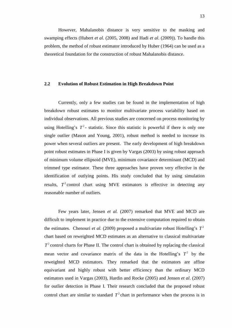
However, Mahalanobis distance is very sensitive to the masking and

swamping effects (Hubert et al. (2005, 2008) and Hadi et al. (2009)). To handle this

problem, the method of robust estimator introduced by Huber (1964) can be used as a

theoretical foundation for the construction of robust Mahalanobis distance.

2.2 Evolution of Robust Estimation in High Breakdown Point

Currently, only a few studies can be found in the implementation of high

breakdown robust estimates to monitor multivariate process variability based on

individual observations. All previous studies are concerned on process monitoring by

using Hotelling’s 2T - statistic. Since this statistic is powerful if there is only one

single outlier (Mason and Young, 2001), robust method is needed to increase its

power when several outliers are present. The early development of high breakdown

point robust estimates in Phase I is given by Vargas (2003) by using robust approach

of minimum volume ellipsoid (MVE), minimum covariance determinant (MCD) and

trimmed type estimator. These three approaches have proven very effective in the

identification of outlying points. His study concluded that by using simulation

results, 2T control chart using MVE estimators is effective in detecting any

reasonable number of outliers.

Few years later, Jensen et al. (2007) remarked that MVE and MCD are

difficult to implement in practice due to the extensive computation required to obtain

the estimates. Chenouri et al. (2009) proposed a multivariate robust Hotelling’s 2T

chart based on reweighted MCD estimates as an alternative to classical multivariate 2T control charts for Phase II. The control chart is obtained by replacing the classical

mean vector and covariance matrix of the data in the Hotelling’s 2T by the

reweighted MCD estimators. They remarked that the estimators are affine

equivariant and highly robust with better efficiency than the ordinary MCD

estimators used in Vargas (2003), Hardin and Rocke (2005) and Jensen et al. (2007)

for outlier detection in Phase I. Their research concluded that the proposed robust

control chart are similar to standard 2T chart in performance when the process is in

14

control and are more efficient than standard 2T chart (with and without outlier

removal in Phase I) when there are outliers in the process during Phase I. The papers

by Midi et al. (2009) and Mohammadi et al. (2011) showed that the use of robust

approaches of MCD, MVE and reweighted MCD in monitoring process is very

significant for detecting changes, compared to the standard approach. Since MVV

give the same robust Mahalanobis distance as FMCD, but with lower computational

complexity, the performance of MVV is better than FMCD.

2.3 High Breakdown Point Robust Estimation Methods

The area of robust statistics has been intensively developed since the sixties.

It is appeared due to the pioneer works of Turkey (1960), Huber (1964), and

Hampel’s idea in 1968 for his PhD research. The term ‘robust’ (strong, sturdy) as

applied to statistical procedures was proposed by Box (1953). The major goal of

robust statistics is to develop methods that are robust against the possibility that one

or several unannounced outliers may occur anywhere in the data. This is the principal

motivation that encourages researchers to develop better methods of robust

estimation of location and scale.

Outlier identification and robust location and scale estimation are closely

related (Werner, 2003). To strengthen this claim, there are a lot of researches in this

area. See, for example, Rousseeuw (1985), Rousseeuw and Zomeran (1990), Hadi

(1992), Becker and Gather (1999), Pena and Prieto (2001), Herwindiati et al. (2007)

and Djauhari et al. (2008).

An application of robust estimates is widely used in industry. See, for

example, in asset allocation (Welsch and Zhou, 2007). In chemical process (Egan

and Morgan, (1998), Wu et al., (2011)), geochemistry exploration (Filzmoser et al.,

2005), wind analysis (Ratto et al., 2012), digital image processing (Vijaykumar et

al., 2009), content based image retrieval (Herwindiati and Isa, 2009), gene intensities

from DNA microarrays (Gottardo et al., 2006), daily mortality and air pollutant

15

concentrations (Wang and Pham, 2011), instrument behaviour study of geothermal

polluted porcelain insulators (Waluyo et al., 2009), manufacturing industry, for

example, Vargas (2003), Chenouri et al. (2009) and Pan and Chen (2010). In this

thesis, the details of the application of robust methods in manufacturing industry will

be presented in Chapter 5.

In the current development of robust location and scale estimation method,

minimum covariance determinant (MCD) is as the basic principle. It is because, as

have mentioned earlier, MCD possesses some commendable properties such as high

breakdown point, bounded influence function, and affine equivariant. The first two

properties ensure that the presence of outliers can only have a small effect on the

estimators. The last property guarantees that the estimators are not affected by any

affine transformation (Hubert et al. 2008). Due to these properties, nowadays FMCD

becomes one of the most widely used robust estimation methods that have received

considerable attention in literature. This method is originally introduced by

Rousseeuw (1985) together with another method called minimum volume ellipsoid

(MVE). However, in recent development, the popularity of MCD dominates that of

MVE. One reason is that, as mentioned in Hadi (1992), MCD is more effective and

efficient than MVE. Moreover, MCD has more attractive geometric interpretation

than MVE.

Since the work of Hadi (1992) who modified MCD to ensure the non

singularity of covariance matrix during iteration process, many papers appeared to

develop MCD. For example, Hawkins (1994) proposed the feasible solution

algorithm (FSA) to satisfy the necessary condition for MCD to be optimum, Hawkins

and Olive (1999) presented a new version of FSA, Croux and Haesbroeck (1999),

studied the influence function of MCD and use it to evaluate the MCD scale

estimator efficiency, Rousseeuw and van Driessen (1999) introduced the so-called

Fast MCD (FMCD) to improve the running time of MCD by introducing the C-step

(data concentration step), Pagnotta (2003) proposed an improvement of FMCD

algorithm by using the agglomerative hierarchical clustering (AHC) to choose the

number of elemental sets, Werner (2003) claimed that FMCD is not apt for high

16

dimension data, and Hubert et al. (2005) improved the performance of FMCD to get

the closer solution to the global optimum.

One of the most recent literature is Hubert and Debruyne (2010) who

mentioned that FMCD procedure is very fast for small sample sizes n , but it works

slower and slower when n gets larger for large p . This statement justified that

Werner’s claim (2003) is true. Those papers focused on covariance determinant or

also known as generalized variance as the stopping rule in C-step. However, in this

step, the optimality criterion of this method is still quite cumbersome if the number

of variables p is large (Djauhari et al., 2008).

To improve the running time of FMCD, Djauhari et al. (2008) introduced

minimum vector variance (MVV) as a new stopping rule in C- step. As mentioned by

Neykov et al. (2011), this method is the refinement step of FMCD constructed for

computational efficiency. It has significantly lower computational complexity. More

specifically, it gives the same robust Mahalanobis distance as FMCD and its

computational complexity is of order ( )2O p while the former is ( )3O p . This is a far

significant improvement in terms of computational complexity for p > 2.

Furthermore, MVV is simple to compute (Wilcox, 2012). However, as will be

discussed in Chapter 4, other criteria of the stopping rule which give the same robust

Mahalanobis distance with lower running time will be developed. For that purpose,

the theoretical foundation of FMCD and MVV will be highlighted in order to show

the advantages of both methods.

2.4 Scenarios in Monitoring Process Variability

In general, monitoring process variability in multivariate setting can be

classified into 3 scenarios. The most common scenario is based on sub-group

observations where the subgroup size, m, is greater than the number of quality

characteristics, p. The details can be found in Alt and Smith (1988), Tang and

Barnett (1996), Yeh et al. (2004), Djauhari (2005), Djauhari et al. (2008), Yeh et al.

17

(2006) and Djauhari and Mohamad (2010). The second scenario is based on

individual observations, i.e. the subgroup size, m is equal one. The main problem of

this scenario is to test the effect of an additional observation on a covariance

structure. The idea of this effect can be seen, for example, in Sullivan and Woodall

(1996), Khoo and Quah (2003), Huwang et al. (2007), Mason et al. (2009, 2010) and

Djauhari (2010, 2011b). The last and the most recent scenario is introduced by

Mason et al. (2009) based on sub-group observations where1 m p< < . As mentioned

earlier, only the second scenario is discussed in this thesis.

2.4.1 Individual Observations-Based Monitoring

In this scenario, we can see many different contributions given by the

authors. For example, Sullivan and Woodall (1996) proposed to use the successive

different on a covariance matrix estimator which is originally introduced by Holmes

and Mergen (1993). Then, Sullivan and Woodall (1996) modified the Hotelling’s T2

statistic by implementing that estimator. They showed that the modified T2 control

chart is more effective than the usual one. Later on, Khoo and Quah (2003) proposed

a simple way for monitoring shifts in the covariance matrix of a p -dimensional

multivariate normal process distribution. In their research, it is assumed that the

process covariance matrix is known. In this case, Phase I operation is not needed.

Huwang et al. (2007) proposed two new control charts, namely the

multivariate exponentially weighted mean squared deviation (MEWMS) and

multivariate exponentially weighted moving variance (MEWMV). Both charts are

constructed based on the trace of the estimated covariance matrices derived from the

individual observations.

Djauhari (2010) proposed another multivariate dispersion measure to monitor

process variability based on individual observations. It is constructed based on the

matrix D defined as the scatter matrix issued from augmented data set (ADS)

subtracted by that from HDS. Specifically, Djauhari’s F statistic, defined as the

18

Frobenius norm of D , represents the effect of additional observations on the

covariance structure. Furthermore, Djauhari (2011b) described that Wilks’ W

statistic is important in the area of industrial application because it has direct, simple

geometrical interpretation and easy to implement in practise especially when p is

not too large. Still, Wilks’ W statistic alone might not be sufficient to describe the

effect of an additional observation on covariance structure. This statistic has serious

limitations as mentioned in Alt and Smith (1988), Montgomery (2005) and Djauhari

(2005, 2010). Djauhari’s F statistic is used to handle the limitations of Wilks’ W

statistic.

2.4.2 Opportunity for Improvement

Actually, W statistic and F statistic are two different measures to quantify the

effect of an additional observation to the covariance structure. Therefore, they have

different properties. In Chapter 5, a monitoring procedure by using both W chart and

F chart separately to construct a more sensitive Phase II operation will be developed.

2.5 Summary

This chapter discussed on the literature study of previous developments and

contributions by other researchers in the development of robust estimation method

and the development of monitoring process variability especially in the scenario of

individual observation based monitoring. The evolution of robust estimation in high

breakdown point and its current development was discussed and it motivates us to

propose a new idea that will be presented in Chapter 4. Then, in order to have a

better understanding of existing measures of process variability of GV and VV,

Chapter 3 will discuss about it in details.

CHAPTER 3

UNDERSTANDING PROCESS VARIABILITY

There is no single measure that can be used to understand process variability

either in univariate setting or multivariate setting because of its complexity

(Djauhari, 2011c). In univariate setting, there are several tools to measure process

variability. For example, range, inter-quartile range, mean absolute deviation,

variance and standard deviation. The covariance matrix Σ is a multivariate

generalization of the univariate concept of variance, 2σ . To measure the multivariate

variability, it is convenient to have a single number rather than a matrix (Mardia et

al., 1979). The most popular and widely used measure is the generalized variance

(GV) or also called covariance determinant, total variance (Chatterjee and Hadi,

1998; Mardia et al., 1979), effective variance (Serfling, 1980; Pena and Rodriguez,

2005), the square root of generalized variance (Alt and Smith, 1988; Djauhari, 2005)

and the relative generalized variance (Tang and Barnett, 1996), and the new

alternative measure called vector variance (VV) (Djauhari, 2007). It should be noted

here that effective variance, square root of generalized variance, and the relative

generalized variance are a function of GV. Since total variance does not involve the

covariance structure, in what follows we concentrate only on GV and VV. However,

these two measures are unable to represent the whole structure of covariance matrix

because they are only a scalar representation of complex structure of covariance

matrix. This shows how difficult to measure and thus to understand multivariate

variability. Although it is difficult to measure the multivariate variability, these

measures are still commonly used to test the equality of two covariance matrices

(Anderson, 1984), to monitor the stability of covariance structure by using GV

(Montgomery, 2005) and by using VV (Djauhari et al., 2008). In Section 3.1, the

20

interpretation of the structure of covariance matrix will be explored in details. The

limitations of GV will be discussed in Section 3.2 as well as the limitations of VV in

Section 3.3. Then, in the last section a way to handle those obstacles in C-step in

FMCD and MVV is highlighted.

3.1 Structure of Covariance Matrix

The structure of multivariate data is hidden in a two dimensional array that

can be presented in n p× matrix X where p is the number of variables and n is the

number of observations on p variables. The following X matrix contains the

information of n observations on p variables; ijX is the measurement of the i-th

individual observation on j-th variable.

X =

11 12 1 1

21 22 2 2

1 2

1 2

j p

j p

i i ij ip

n n nj np

X X X XX X X X

X X X X

X X X X

.

This data matrix can be considered from two points of view. First, each row

is a vector of individual observation in a space of p dimension pR . Second, each

column is a vector of individual variable in nR . If X is the sample mean vector,

X = 1

1 n

ii

Xn =∑

then ( )( )'

1

n

i ii

A X X X X=

= − −∑ is the scatter matrix and 11

S An

=−

is the sample

covariance matrix which is an unbiased estimate of the population covariance matrix

21

11 12 1

21 22 2

1 2

p

p

p p pp

σ σ σ σ σ σ ∑ = σ σ σ

.

Let us write

11 12 1

21 22 2

1 2

p

p

p p pp

s s ss s s

S

s s s

=

.

The element iis is the sample variance of the i-th variable. It can be

considered as the squared norm of the centred i-th variable divided by ( )1n − .

Furthermore, the sample covariance of the i-th and j-th variables, ijs , is the scalar

product of the centred i-th and j-th variables divided by the same scalar. Therefore,

from Linear Algebra, we know that the sample correlation

ijij

ii jj

sr

s s=

is nothing more than the cosine of the angle between the centred i-th and j-th point

variables in nR .

The above point of view guides us that the covariance matrix S represents

the configuration of p variables in that space defined by the norm (length) of each

variable and the angle between two different point variables.

If we write the sample correlation matrix

R =

11 12 1

221 22

1 2

p

p

p p pp

r r rrr r

r r r

,

then R is the estimated of population correlation matrix

22

11 12 1

221 22

1 2

p

p

p p pp

ρ ρ ρ

ρρ ρ Ω = ρ ρ ρ

.

3.2 Understanding the Role of GV

A major role of total variance (TV) generally can be found easily in the

problem of data dimension reduction such as, for example, in the principal

component analysis, (Anderson (1984) and Johnson and Wichern (2007)), and

canonical correlation analysis (Anderson (1984)). This limitation of the role of TV in

application is understandable because it involves the variance only without involving

the whole structure of covariance. In other words, it is simply involving the diagonal

elements of covariance matrix.

Meanwhile, the role of GV can be found in every literature on multivariate

analysis particularly in testing hypothesis of two or more covariance structures

equality and multivariate dispersion monitoring. See, for example, Kotz and Johnson

(1985), Alt and Smith (1988), Montgomery (2005) and Djauhari (2005). The role of

GV also can be found in FMCD and minimum volume ellipsoid (MVE); the two

robust estimation methods of location and scatter (Rousseeuw, 1985).

The GV provides a way of writing, in the form of scalar representation, the

information about covariance structure. Since it is only a scalar representation then it

could happen that two different covariance matrices have the same GV. As an

illustration, consider the three covariance matrices:

1

4 00 4

Σ =

, 2

5 33 5

Σ =

, 3

5 33 5

− Σ = −

.

23

The value of GV of those covariance matrices is the same, i.e.,

1 2 3 16Σ = Σ = Σ = . The three matrices convey considerably different information

about covariance structure. The variables represented in 1Σ are independent of each

other, but they are positively and negatively correlated according to 2Σ and 3Σ ,

respectively. Therefore, those different correlation structures cannot be distinguished

by GV. See Johnson and Wichern (2007), Mason et al. (2009), and Djauhari and

Mohamad (2010) for further discussion.

A geometrical representation of bivariate normal probability density function

(PDF) with zero mean vector and those three covariance matrices will help us to

understand what covariance structure is. In order to show the difference of

covariance structure among 1Σ , 2Σ and 3Σ , the 3-d image of that PDF is plotted.

Figure 3.1 Bivariate normal PDF with 1

4 00 4

Σ =

24


5 33 5

Σ =

.


5 33 5

− Σ = −

.

On the other hand, if the graph is sliced horizontally, the confidence ellipse

will be obtained. The view from the surface will be like Figure 3.4 to Figure 3.6.

REFERENCES Alt, F. B. and Smith, N. D. (1988). Multivariate Process Control. In Krishnaiah, P.

R., Rao, C. R. (Ed.) Handbook of Statistics (pp. 333–351). Elsevier Science.

Anderson, T. W. (1984). Introduction to Multivariate Statistical Analysis, Second

Edition, Wiley-Interscience: New York.

Aho. A. V., Hopcroft. J. E., and Ullman, J. D. (1983). Data Structures and

Algorithms. Addison-Wesley Publishing Company: California.

Barnett, V., and Lewis, T. (1984). Outliers in Statistical Data. 2nd edition. New

York: John Wiley.

Becker, C. and Gather, U. (1999). The Masking breakdown Point of Multivariate

Outlier Identification Rules. Journal of the American Statistical Association.

94(447): 947-955.

Box, G. E. P. (1953). Non-normality and Test on Variances. Biometrika. 40(3/4):

318-335.

Chai, I. and White, J. D. (2002). Structuring Data and Building Algorithms.

McGraw-Hill: Malaysia.

Chakraborti, S., Human, S. W. and Graham, M. A. (2008). Phase I Statistical Process

Control Charts: An Overview and Some Results. Quality Engineering. 21(1):

52-62.

Chatterjee, S. and Hadi, A. S. (1988), Sensitivity Analysis in Linear Regression. New

York : John Wiley & Sons.

Chenouri, S., Steiner, S. H. and Variyath, A. M. (2009). A Multivariate Robust

Control Chart for Individual Observations. Journal of Quality Technology.

41(3): 259-271.

Croux, C. and Haesbroeck, G. (1999). Influence Function and Efficiency of the

Minimum Covariance Determinant Scatter Matrix Estimator. Journal of

Multivariate Analysis. 71 : 161-190.

121

Djauhari, M. A. (1999). An Exact Test for Outlier Detection. BioPharm

International: The Applied Technology of Biopharmaceutical Development.

12(6): 56-59.

Djauhari, M.A. (2002). Mahalanobis Distance From MANOVA Point of View and Its

Generalization for Handling Masking and Swamping Effects in Drug Analysis.

Final Report of the Tenth Competitive Grant. Institut Teknologi Bandung.

Djauhari, M. A. (2003). Statistical Testing for Outliers: Calculating the Critical Point

of the Extreme Studentized Deviation Using the Beta Inverse Function.

BioPharm International: The Applied Technology of Biopharmaceutical

Development. 16(10): 60-68.

Djauhari, M. A. (2005). Improved Monitoring of Multivariate Process Variability,

Journal of Quality Technology. 37(1): 32-39.

Djauhari, M. A. (2007). A Measure of Multivariate Data Concentration. Journal of

Applied Probability & Statistics. 2(2): 139-155.

Djauhari, M. A. (2010). A Multivariate Process Variability Monitoring Based on

Individual Observations. Journal of Modern Applied Science. 4(10): 91-96.

Djauhari, M. A. (2011a). Strategic Roles of Industrial Statistics in Modern Industry.

ASM Science Journal. 5(1): 53-63.

Djauhari, M. A. (2011b). Manufacturing Process Variability: A Review. ASM

Science Journal. 5(2): 123-137.

Djauhari, M. A. (2011c). Geometric Interpretation of Vector Variance.

MATEMATIKA, 27(1): 51-57.

Djauhari, M. A. and Mohamad, I. (2010). How to Control Process Variability More

Effectively: The case of a B-Complex Vitamin Production Process. South

African Journal of Industrial Engineering. 21(2): 207-215.

Djauhari, M. A., Mashuri, M. and Herwindiati, D. E. (2008). Multivariate Process

Variability Monitoring. Communications in Statistics-Theory and Methods. 37:

1742-1754.

Donoho, D. L. and Huber, P. J. (1983). The Notion of Breakdown Point. In Bickel,

P. J., Doksum, K. A. ad Hodges, J. L. (Ed.) A Festschrift for Eric Lehmann.

Belmont, CA: Wadsworth.

Dykstra, R. L. (1970). Establishing the Positive Definiteness of the Sample

Covariance Matrix. The Annals of Mathematical Statistics. 41(6): 2153-2154.

122

Egan, W. J. and Morgan, S. L. (1998). Outlier Detection in Multivariate Analytical

Chemical Data. Analytical Chemistry. 70(11): 2372-2379.

Escoufier, Y. (1973). Le traitement des Variables Vectorielles. Biometrics. 29: 751 –

760.

Escoufier, Y. (1976). Opérateur Associé à un Tableau de Données. Annales de

l’INSEE. 22-23: 342 – 346.

Erbacher, R. F., Walker, K. L. and Frincke, D. A. (2002). Intrusion and Misuse

Detection in Large-Scale Systems. Computer Graphics and Applications,

IEEE. 22(1): 38-47.

Filzmoser, P. (2004). A Multivariate Outlier Detection Method.

http://computerwranglers.com/com531/handouts/mahalanobis.pdf- accessed on

December 2011.

Filzmoser, P., Reimann, C. and Garrett. R. G. (2005). Multivariate Outlier

Identification in Exploration Geochemistry. Computers and Geosciences. 31 :

579-587.

Gladwell, M. (2008). Outliers: The Story of Successes. New York: Little, Brown and

Company.

Gnanadesikan, R. and Kettering, J. R. (1972). Robust Estimates, Residuals, and

Outlier Detection with Multi Response Data. Biometrics. 28 (1): 81-124.

Grubbs, F. E. (1950). Sample Criteria for Testing Outlying Observations. Annals of

Mathematical Statistics. 21(1): 27-58.

Grubel, R. (1988). A Minimal Characterization of the Covariance Matrix. Metrika.

35:49-52.

Gottardo, R., Raftery, A. E., Yeung, K. Y. and Bumgarner, R. E. (2006). Quality

Control and Robust Estimation for cDNA Microarrays With Replicates.

Journal of the American Statistical Association. 101(473): 30-40.

Hadi A. S. (1992). Identifying Multivariate Outliers in Multivariate Data. Journal of

Royal Statistical Society B. 53: 761-771.

Hadi, A. S., Imon, A. H. M. R., and Werner, M. (2009). Detection of Outliers.

WIREs Computational Statistics. 1: 57-70.

Hardin, J. and Rocke, D. M. (2005). The Distribution of Robust Distances. Journal

of Computational and Graphical Statistics. 14(4): 928 – 946.

Hawkins, D. M. (1994). The Feasible Solution Algorithm for the MCD Estimator.

Journal of Computational Statistics and Data Analysis. 17: 197-210.

123

Hawkins, D. M. and Olive, D. J. (1999). Improved Feasible Solution Algorithm for

High Breakdown Estimation. Journal of Computational Statistics and Data

Analysis. 30: 1-11.

Herdiani, E. T. (2008). A Statistical Test for Testing the Stability of a Sequence of

Correlation Matrices. PhD Thesis, Department of Mathematics, Institut

Teknologi Bandung, Indonesia.

Herwindiati, D. E., Djauhari, M. A. and Mahsuri, M. (2007). Robust Multivariate

Outlier Labelling. Journal of Communication in Statistics - Computation and

Simulation, 36: 1287-1294.

Herwindiati, D. E., and Isa, S. M. (2009). The Robust Distance for Similarity

Measure of Content Based Image Retrieval. Proceedings of the World

Congress on Engineering 2009. July 1-3. London ,UK: WCE Vol II.

Holmes, D. S. and Mergen, A. E. (1993). Improving the Performance of the T2-chart.

Quality Engineering. 5(4): 619-625.

Hubert, M. and Debruyne, M. (2010), Minimum Covariance Determinant. WIREs

Computational Statistics. 2.

Hubert, M., Rousseeuw, P. J. and van Aelst, S. (2008). High-Breakdown Robust

Multivariate Methods. Statistical Science, 23(1): 92-119.

Hubert, M., Rousseeuw, P.J., and van Aelst, S. (2005). Multivariate Outlier

Detection and Robustness. Handbook of Statistics, Edition 24. Elsevier. 263-

302.

Huber, P. J. (1964). Robust Estimation of Location Parameter. Annals of

Mathematical Statistics. 35: 73-101.

Huwang, L., Yeh, A. B. and Wu, C. W. (2007). Monitoring Multivariate Process

Variability for Individual Observations. Journal of Quality Technology. 39(3):

258-278.

Iglewicz, B. and Hoaglin, D. C. (1993). How to Detect and Handle with Outliers.

Milwaukee: ASQ Press.

Jensen, W. A., Birch, J. B. and Woodall, W. H. (2007). High Breakdown Point

Estimation Methods for Phase I Multivariate Control Charts. Quality and

Reliability Engineering International. 23(5): 615-629.

Johnson, R. A. and Wichern, D. W. (2007). Applied Multivariate Statistical Analysis.

6th Edition. New York: John Wiley.

124

Kennedy, G. C., Matsuzaki, H., Dong, S., Liu, W. M., Huang, J., Liu, G., Su, X.,

Cao, M., Chen, W., Zhang, J., Liu, W., Yang, G., Di, X., Ryder, T., He, Surti,

U., Philips, M. S., Boyce-Jacino, M. T., Fodor, S. P., and Jones, K. W. (2003).

Large-Scale Genotyping of Complex DNA. Nature Biotechnology. doi:

10.1038/nbt869.

Khoo, M. B. C. and Quah, S. H. (2003). Multivariate Control Chart for Process

Dispersion Based on Individual Observations. Quality Engineering. 15(4): 639-

642.

Koutsofios, E. E., North, S. C. and Keim, D. A. (1999). Visualizing Large

Telecommunication Data Sets. Computer Graphics and Applications, IEEE. 19

(3): 16-19.

Kotz, S. and Johnson, N. L. (1985). Encyclopedia of Statistical Sciences, Edition 6.

New York: John Wiley.

Mardia, K. V., Kent, J. T. and Bibby, J. M. (1979). Multivariate Analysis. London:

Academic Press.

Maronna, R. A., Martin, R. D. and Yohai, V. J. (2006). Robust Statistics: Theory and

Methods. West Sussex, England: John Wiley & Sons Ltd.

Mason, R. L. and Young, J. C. (2001). Implementing Multivariate Statistical Process

Control Using Hotelling’s T2 Statistic. Quality Progress, April: 71-73.

Mason, R. L. and Young, J. C. (2002). Multivariate Statistical Process Control with

Industrial Applications, Philadelphia: ASA-SIAM.

Mason, R. L., Tracy, N. D. and Young, J. C. (1995). Decomposition for Multivariate

Control Chart Interpretation. Journal of Quality Technology. 27(2): 99-108.

Mason R. L., Chou, Y. M. and Young, J. C. (1996). Monitoring a Multivariate Step

Process. Journal of Quality Technology. 28(1): 39-50.

Mason R. L., Chou, Y. M. and Young, J. C. (2009). Monitoring Variation in a

Multivariate Process When the Dimension is Large Relative to the Sample

Size, Communication in Statistics – Theory and Methods. 38: 939-951.

Mason R. L., Chou, Y. M. and Young, J. C. (2010). Decomposition of Scatter Ratios

Used in Monitoring Multivariate Process Variability. Communication in

Statistics – Theory and Methods. 39: 2128-2145.

Mason R. L., Chou, Y. M. and Young, J. C. (2011). Detection and Interpretation of a

Multivariate Signal Using Combined Charts. Communication in Statistics –

Theory and Methods. 39: 942-957.

125

Mason R. L., Champ, C. V., Tracy, N. D., Wierda, S. J. and Young, J. C. (1997).

Assessment of Multivariate Process Control Techniques; A Discussion on

Statistically-Based Process Monitoring and Control. Journal of Quality

Technology. 29(2): 140-143.

Mason R. L., Chou, Y. M., Sullivan, J. H., Stroumbos, Z. G. and Young, J. C.

(2003). Systematic Pattern in T2 Chart. Journal of Quality Technology. 35(1):

47-58.

Midi, H., Shabbak, A., Talib, B. A. and Hassan M. N. (2009). Multivariate Control

Chart Based on Robust Mahalanobis Distance. Proceedings of the 5th Asian

Mathematical Conference, Malaysia.

Mohammadi, M., Midi, H., Arasan, J. and Al-Talib, B. (2011). High Breakdown

Estimators to Robustify Phase II Multivariate Control Charts. Journal of

Applied Sciences. 11(3): 503-511.

Montgomery, D. C. (2005). Introduction to Statistical Quality Control. 5th edition.

New York: John Wiley and Sons, Inc.

Neykov, N. M., Filzmoser, P., and Neytchev, P. N. (2012). Robust Joint Modelling

of Mean and Dispersion through Trimming. Computational Statistics and Data

Analysis. 56: 34-48.

Pagnotta, S. M. (2003). An Improvement of the FAST-MCD Algorithm.

http://www.stat.unisannio.it/Pagnotta/paper/SIS2003.pdf - accessed on 23

December 2010.

Pan, J. N. and Chen, S. C. (2010). New Robust Estimators for Detecting Non-

Random Patterns in Multivariate Control Charts: A Simulation Approach.

Journal of Statistical Computation and Simulation. 81(3): 289-300.

Pena, D. and Preito, J. F. (2001). Multivariate Outlier Detection and Robust

Covariance Matrix Estimation. Technometrics. 43(3): 286-300.

Prins, J. and Mader, D. (1997). Multivariate Control Charts for Grouped and

Individual Observations. Quality Engineering. 10(1): 49-57.

Ratto, G. Maronna, R., Repossi, P., Videla, F., Nico, A. and Almandos, J. R. (2012).

Analysis of Wind Affecting Air Pollutant Transport at La Plata, Argentina.

Atmopheric and Climate Sciences. 2: 60-75.

Reingold, E. M. (1999). Algorithm Design and Analysis Techniques. In: Atallah M.

J. (Ed). Algorithms and Theory of Computational Handbook (pp.1-27). CRC

Press: Florida.

126

Rosner, B. (1975). On the Detection of Many Outliers. Technometrics. 17(2): 221-

227.

Rousseeuw, P. J. (1985). Multivariate Estimation with High Breakdown Point. In:

Grossman, B. W., Pflug, G., Vincze, I., Wertz, W. (Ed). Mathematical

Statistics and Applications (pp. 283 – 297). D. Reidel Publishing Company.

Rousseeuw, P. J. and Leroy, A. M. (1987). Robust Regression and Outlier Detection.

John Wiley: New York.

Rousseeuw, P. J. and van Driessen, K. (1999). A Fast Algorithm for the Minimum

Covariance Determinant Estimator. Technometrics, 41(3): 212 – 223.

Rousseeuw, P. J. and van Zomeren, B. C. (1990). Unmasking Multivariate Outliers

and Leverage Points. Journal of the American Statistical Association. 85(411):

633-639.

Rousseeuw, P. J. and van Zomeren, B. C. (1991). Robust Distances: Simulations and

Cut-off Values. In Stahel, W. and Weigberg, S. (Ed.) Directions in Robust

Statistics and Diagnostics, Part II, The IMA Volumes in Mathematics and Its

Applications. 34: 195-203. New York: Springer-Verlag.

Ryan, T. P. (2011). Statistical Methods for Quality Improvement, 3rd edition. John

Wiley & Sons, Inc.: New Jersey

Seber, G. A. F. (1984). Multivariate Observations. John Wiley & Sons, Inc.: New

York.

SEMATECH, USA. http://www.itl.nist.gov/div898/handbook/index.htm. National

Institute Science and Technology. Accessed on July 2004.

Serfling, R.J. (1980). Approximation Theorems of Mathematical Statistics. New

York: John Wiley.

Sullivan, J. H. and Woodall, W. H. (1998). Adapting Control Charts for the

Preliminary Analysis of Multivariate Observations. Communication in

Statistics – Simulation and Computation. 27: 953-979.

Sullivan, J. H. and Woodall, W. H. (1996). A Comparison of Multivariate Control

Charts for Individual Observation. Journal of Quality Technology. 28(4): 398-

408.

Tang, P. F. and Barnett, N. S. (1996). Dispersion Control for Multivariate Processes.

Austral. J. Statist., 38(3): 235-251.

Tietjen, G. L. and Moore, R. H. (1972). Some Grubbs-Type Statistics for the

Detection of Several Outliers, Technometrics. 14(3): 583-597.

127

Thompson, W. R. (1935). On a Criterion for the Rejection of Observations and the

Distribution of the Ratio of Deviation to Sample Standard Deviation. Annals of

Mathematical Statistics. 6(4): 214-219.

Tracy, N. D. and Young, J. C. (1992). Multivariate Control Charts for Individual

Observations. Journal of Quality Technology. 24: 88-95.

Tukey, J. W. (1977). Exploration Data Analysis. Wesley Canada: Addison.

Tukey, J. W. (1960). A Survey of Sampling from Contaminated Distributions. In

Olkin, I. (Ed.) Contributions to Probability and Statistics (pp. 448-485).

Stanford: Stanford Univ. Press.

Vargas, J. A. (2003). Robust Estimation in Multivariate Control Charts for Individual

Observations. Journal of Quality Technology. 35(4): 367-376.

Vijaykumar, V. R., Vanathi, P. T., Kanagasabapathy, P. and Ebenezer, D. (2009).

Robust Statistics Based Algorithm to Remove Salt and Pepper Noise in

Images. International Journal of Information and Communication

Engineering. 5(3) : 164-172.

Waluyo, Sinisuka, N. I., Suwarno, and Djauhari, M. A. (2009). Robust Canonical

Correlation Analysis on Leakage Current Behaviors of Geothermal Polluted

Porcelain Insulators. Jurnal Ilmiah Semesta Teknika. 12(2):132-146.

Wang, Y. and Pham, H. (2011). Analyzing the Effects of Air Pollution and Mortality

by Generalized Additive Models With Robust Principal Components.

International Journal of System Assurance Engineering and Management.

2(3):253-259.

Welsch, R. E. and Zhou, X. (2007). Application of Robust Statistics to Asset

Allocation Models. REVSTAT-Statistical Journal. 5(1): 97-114.

Werner, M. (2003). Identification of Multivariate Outliers in Large Data Sets.

Doctor Philosophy, University of Colorado, Denver.

Wierda S. J. (1994). Multivariate Statistical Process Control – Recent Results and

Directions for Future Research. Statistica Neerlandica. 48(2):147-168.

Wilcox, R. (2012). Introduction to Robust Estimation and Hypothesis Testing. 3rd

Edition. Elsevier. Printed in USA.

Wilks, S. S. (1962). Mathematical Statistics. New York: John Wiley & Sons, Inc.

Wilks, S. S. (1963). Multivariate Statistical Outliers. Sankhya: The Indian Journal of

Statistics, 25(4): 407-426.

128

Woodall, W. H. and Montgomery, D. C. (1999). Research Issues and Ideas in

Statistical Process Control. Journal of Quality Technology. 31(4): 376-386.

Wu, G., Chen, C., and Yan, X. (2011). Modified Minimum Covariance Determinant

Estimator and Its Application to Outlier Detection of Chemical Process Data.

Journal of Applied Statistics. 38(5): 1007-1020.

Yanez, S., Gonzalez, N. and Vargas, J. A. (2010). Hotelling’s T2 Control Chart

Based on Robust Estimators. Dyna 77(163): 239-247.

Yeh, A. B., Huwang, L., and Wu, Y. F. (2004). A Likelihood-Ratio-Based EWMA

Control Chart for Monitoring Variability of Multivariate Normal Processes.

IIEE Transaction. 36: 865-879.

Yeh, A. B., Lin, D. K. and Mc Grath, R. N. (2006). Multivariate Control Chart for

Monitoring Covariance Matrix. Quality Technology & Quantitative

Management, 3: 415-436.

a robust estimation method of location and scale

Documents