a robust optimization modeling for mine supply chain

Research ArticleA Robust Optimization Modeling for Mine Supply ChainPlanning under the Big Data

Wenbo Liu

Department of Logistics Management, Liaoning Provincial College of Communications, Shenyang 110122, China

Correspondence should be addressed to Wenbo Liu; [email protected]

Received 12 August 2021; Accepted 27 September 2021; Published 23 October 2021

Academic Editor: Rajesh Kaluri

Copyright © 2021 Wenbo Liu. This is an open access article distributed under the Creative Commons Attribution License, whichpermits unrestricted use, distribution, and reproduction in any medium, provided the original work is properly cited.

With the rapid development of information technology, large-scale data is collected and stored, which provides a huge amount ofinformation for decision-making. This paper focuses on the planning of mine supply chain under the big data. The mine supplychain usually contains three stages, which is mining, processing, and ore product transportation. This paper tackles the difficultyof variable cut-off grade by establishing a robust optimization model. To solve the robust optimization model, the nonlinearconstraints in the model were linearized first. Then, the specific parameter values were determined through the employment ofthe hypothesis test in statistics, and the robust optimization model was solved finally. The analysis results show that the robustoptimization model can be stabilized when the parameters are subject to disturbance. Finally, sensitivity analysis experimentsare carried out for several parameters in the model to find out the influence of each parameter on the model. This papercombines mine supply chain planning with big data, which not only improves the production and transportation efficiency ofore products, but also reduces related costs.

1. Introduction

The steel industry is an important basic industry sector,which is the material base of developing national economyand national defense construction. It consumes large amountof iron ores in daily production and thus tends to maintain ahigh level of inventory. Meanwhile, the mining companies,which provide the iron ores suffer from the uncertainty ofore grade in mining and the market fluctuations in transpor-tation. Based on this, it is necessary to establish a long-term,stable, and safe mine supply chain.

The mine supply chain under big data involves manylinks and contains a large number of relevant data or param-eters. The emergence of big data has an unmistakable impacton the amount and speed of data processed in supply chains[1–3]. In the mine supply chain, the raw ores are extractedfrom multiple mining locations first, and each of the locationmight have different ore grade. Then, the raw ores are mixedto meet the ore grade requirements and then transport to theconcentrating mills for processing. Finally, the ore productsare transported through railway or sea transportation fromthe concentrating mills to the logistics centers. The demands

of the final users are met by the accurate services of the logis-tics centers. During the whole mine supply chain, the oregrade is a key factor involved in the decision-making. Foreach mining location, based on the estimation of the naturalore grade, the manager must determine a cut-off grade tooptimize the quality and quantity of the mined ore. Gener-ally speaking, the higher the cut-off grade, the higher theore quality while the lower the ore quantity, since the ironore blocks with a natural ore grade lower than the cut-offgrade is dumped as waste. The concentrating mill has aminimum ore grade for the raw ore, and the decision ofthe cut-off grades in multiple ore locations will be subjectto the mining of the iron ore, as well as the correspondingprocessing, inventory, and transportation largely. In thispaper, the variable cut-off grade, which varies in differenttime periods is considered, for the purpose of promotingthe flexibility of the whole ore supply chain. Most of the pre-vious research attaches importance to the solution to a singlecomponent of the mine supply chain, e.g., mining, process-ing, production, warehousing, or transportation. It is of greatsignificance to study the whole mine supply chain, which iscomposed of the entire process of production, processing,

HindawiWireless Communications and Mobile ComputingVolume 2021, Article ID 1709363, 11 pageshttps://doi.org/10.1155/2021/1709363

https://orcid.org/0000-0003-0493-8613

https://creativecommons.org/licenses/by/4.0/

https://doi.org/10.1155/2021/1709363

inventory, and transportation. Mine supply chain planningis a data-driven process that focuses on developing plans tooperate the supply chain efficiently and optimizing out-comes under given constraints [4]. Big data analysis toolssuch as optimization algorithms can help the supply chainto balance resource and to determine reasonable productionplanning capabilities, inventory levels, distribution capabili-ties, etc. [5, 6].

We followed the modeling methods of Liu et al. [7] andbuilt a robust optimization model based on the importantparameter of the cut-off grade. It was the logic of this paperthat firstly determined the range of the parameter by the sta-tistical analysis for the ore grade parameters through theemployment of actual observation and exploration results,and then helped obtain the value of the relevant parametersby using hypothesis testing. Hypothesis testing with statisti-cal significance is one of the most important methods of bigdata analysis. In addition, the objective function valuesobtained by the robust optimization model were comparedwith each other by carrying out numerical experiments,and then the verification for the stability and optimality ofthe robust optimization model was performed. As for robustoptimization, it was able to address the problem of datauncertainty by guaranteeing the feasibility and optimalityof the solution for the worst instances of the parameters.Through a number of numerical experiments, it was shownby the experimental results that the proposed robust optimi-zation model was very stable under the circumstance ofparameter perturbations.

This paper is aimed at coordinating mining, inventory,and transportation between all the aspects of the minesupply chain under the premise of considering relevantconstraints and minimizing the total costs on the mining,blending, processing, inventory, and transportation of thesupply chain. The main contribution of this paper is to inte-grate the key node enterprises in the mine supply chain, theoptimization of its production and logistics systems, reduceor eliminate the phenomenon of unbalanced production,avoid the fluctuation of upstream and downstream, makethe ore mining, processing, and transportation orderly, andrealize the balanced development of supply and demand,so as to improve the overall benefit and efficiency of themine supply chain. The research objects of this paperinclude monomer ore and other multimetal.

This paper is organized as follows: In Section 2, wereview relevant literature. Section 3 describes our problemand constructs a robust optimization model. In Section 4,performance analysis and sensitivity analysis experimentsare carried out for the robust optimization model. It is veri-fied by the numerical experiments that the robust optimiza-tion model is able to meet the actual needs and obtain idealresults. Section 5 concludes the paper.

2. Literature Review

Ghiani et al. [8] defined the supply chain as “a complexlogistics system in which raw materials are converted intofinished products and then distributed to final users(consumers or companies).” The competitive advantage of

supply chain management in various industries is realizedthough supply chain planning [9]. The supply chain plan-ning involves many functional areas of procurement,production and distribution, and across strategic networkplanning, production planning and scheduling, purchasingand material requirement planning, and distribution andtransport planning [6, 10]. Brunaud and Grossmann [11]put forward the statement that some researchers carriedout relevant studies on the supply chain modeling and opti-mization issues in a variety of industries. Nishi et al. [12]proposed a framework for distributed optimization of supplychain planning and coordination approach. Steinrücke [13]studied the practical problems of the global aluminum forsupply chain network. Members of the aluminum for supplychain network are scattered around the world. They con-structed a novel type of mixed-integer decision-makingmodel, which can coordinate the production quantities andtimes of all supply chain members, in order to minimizethe production and transportation cost of the whole supplychain. Vintró et al. [14] and Söderholm et al. [15] focusedtheir research on green supply chain, such as the issuesrelated to the society, environment, health, and safety. Apartfrom that, Kusi-Sarpong et al. [16] fixed their attention onthe studies carried out for a framework and evaluation ofGhana’s mining green supply chain practices. Azapagic[17] devoted himself to the development of a frameworkfor the sustainable development of the mining and miningindustry, in which economic, environmental, social, andother comprehensive indicators for the mining industrystakeholders are included.

Big data analysis is highly relevant to supply chain plan-ning [5]. Optimization techniques can provide fundamentalsupport to demand planning, production planning, inven-tory plans, and logistics planning by improving planningaccuracy and flexibility [18–20]. The big data is collectedfrom a wide range of diversified sources with various per-spectives and data formats (i.e., variety) [21]. The digitiza-tion of supply chains [22] for better tracking of supplychains further highlights the role of big data analytics. Heet al. [23] carried out some researches in the fields of big dataanalysis, which used dimensionality reduction algorithm ofbig data to quickly extract valuable parts from a hugeamount of data and improve computational efficiency.

The production and distribution logistics planning in theopen pit mine is known for its own unique features of themining industry. It is the uncertainty available in the qualityrequirements of ore iron concentrates that challenges thechoice about which grade of ore to mine. Newman et al.[24] review several decades of literature, including minedesign, long-term and short-term production scheduling,equipment selection, and dispatching. Chen and Wang[25] constructed a linear programming model for integratedproduction planning for Canadian steel making company.The production plan is considered as an integrated process,including raw material procurement, semi-finished productprocurement, capacity allocation, and finished product pro-duction and distribution. The purpose of the model is tooptimize production planning based on production costs,product throughput rates, customer demands, sales prices,

2 Wireless Communications and Mobile Computing

and facility capacities. Lagos et al. [26] consider a miningproblem involving extraction and processing decisionsunder capacity constraints, and they solved the uncertaintyof the ore grade.

The measure of dealing with uncertainty in supply chainoptimization is usually completed by four commonmethods, stochastic programming (Azaron et al. [27]), fuzzyprogramming (Mitra et al. [28] and Lin et al. [29]), probabi-listic programming (You and Grossmann [30]), and sensi-tivity analysis for instance. Robust optimization (Ben-Taland Nemirovski [31]) is able to provide a framework to han-dle the uncertainty of parameters in the problems related tooptimization within the category of a given set of boundeduncertainties, and the optimal solution can also be offeredin an uncertain implementation. In addition, robust optimi-zation can solve the model with uncertain parameters andrealize the feasibility and optimality of the solution in theworst case of parameters. Bertsimas and Thiele [32]proposed a general robust methodology for the purpose ofsolving the problem of inventory with fixed costs and con-straints of capacity for production/inventory. Gurnani et al.[33] focused on the analysis of a supply chain in assemblysystems, where there was uncertainty in yields and demand.Zahiri et al. [34] proposed a robust model of demand-deterministic supply chain, which was composed of the cen-ters for collection and distribution. Pishvaee et al. [35] fixedtheir attention on the study of a robust optimization modelto manage uncertainty data for the problems existing insupply chain design. Vahdani et al. [36] proposed a reliabledesign model of supply chain in the circumstance of uncer-tainty. They present a dual-objective mathematical program-ming method, which can minimize the total cost andexpected transportation cost under the failure of logisticsnetwork facilities. Additionally, Paydar et al. [37] proposeda MILP model for the used oil supply chain. Based on theuncertainty of oil collection, the robust optimization methodwas proposed by Mulvey et al. [38]. [32] Safaei et al. [39]proposed a mixed integer linear programming model, whichcan be used to optimize the paper and cardboard recyclingnetwork and solve demand uncertainty of the network byusing the robust optimization. Jiao et al. [40] studied thedesign of sustainable closed-loop supply chain in a varietyof uncertain circumstances. They also presented the data-driven approaches to generate robust closed-loop supplychain which can reduce uncertainty. It follows that most ofthe studies conducted previously put emphasis on the mech-anism modeling and failed to set up the supply chain systemfrom the data-driven perspective. Therefore, it is quite diffi-cult to ensure the accuracy of the mechanism model, due tothe subjective factors. In fact, data on relevant industries areeasy to collect because it reflects the objective world.

3. Problem Description and Model

3.1. Problem Description. In recent years, with the continuousincrease of global mining investment and production capacity,the overall supply capacity of ore has been significantlyimproved, which further promotes the continuous increase

of global iron ore production and sea transport. The long-term stability of ore supply chain will attach great importance.

Macroscopically, the relevant nodes of the mine supplychain include mines, concentrating mills, logistics centers,and final users. The efficient operation of mine supply chaincan realize the minimum total cost, including mining, pro-cessing, inventory, and transportation.

Different from general enterprises, mining enterprisesextract ore resources from nature. Each ore body has itsown characteristic; there are significant differences in min-ing technology, methods, and equipment. It is widelybelieved that ore grade is a very important factor in the pro-cess of mining. The production capacity of mine is affectedby the grade distribution of ore body. The fluctuation ofore grade distributed in different orebodies will have a greatinfluence on the output and quality of mined ore and thenaffect the subsequent processing. Therefore, the variablecut-off grade should be considered in the mining plan toallow for the flexibility of the mining stage under productioncapacity constraints. Due to the development of technologyand industry, the quality of mineral requirements is moreand more high, the need for mineral processing of raw ore,which is mineral processing. The mineral processing is themost important section in the whole production of mine. Inaddition, in order to meet the final users’ demand for oreproducts in the supply chain, it is necessary to coordinatethe mining and processing of ore. Therefore, the mine supplychain mentioned in this paper is different from the traditionalsingle (multi) product and single (multi) period supply chain.

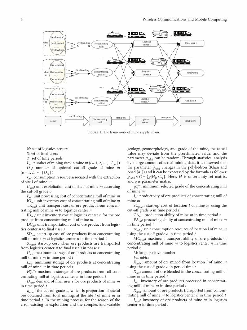
Figure 1 shows the framework of mine supply chain. Oremined from multiple locations needs to be blended to meetthe grade requirements of the concentrating mill. Then, theore products from the concentrating mill will be transportedto logistics centers in batches. According to demand, thelogistics centers will store ore products of specific grades.Finally, the ore product will be transported from the logisticscenters to the final users according to requirements.

The actual assumptions are as follows:

(1) Each mine has a number of ore extraction locationsand can extract a variety of ore grade of raw ore,but the mining capacity of each mine is limited

(2) In each mine, raw ore from different locations istransported to the concentrating mill which belongsto mine for processing, and only one type of oreproducts is produced in the whole process

(3) Ore products of different grade are transported fromthe concentrating mills to logistics centers inbatches, and ore products are then sent to final usersin batches

In the next section, a robust optimization model isproposed.

3.2. Model. A robust optimization model is built based onthe sets, parameters, and variables as follows.

Sets and parametersM: set of concentrating mills corresponding to mines

3Wireless Communications and Mobile Computing

N : set of logistics centersS: set of final usersT : set of time periodsLm: number of mining sites in minem (l = 1, 2,⋯, ∣ Lm ∣ )Om: number of optional cut-off grade of mine m

(o = 1, 2,⋯, ∣Om ∣ )rml : consumption resource associated with the extraction

of site l of mine mCmlo: unit exploitation cost of site l of mine m according

the cut-off grade oPm: unit processing cost of concentrating mill of mine mIOm: unit inventory cost of concentrating mill of mine mTRmn: unit transport cost of ore product from concen-

trating mill of mine m to logistics center nIDmn: unit inventory cost at logistics center n for the ore

product from concentrating mill of mine mDCns: unit transportation cost of ore product from logis-

tics center n to final user sSDmnt : start-up cost of ore products from concentrating

mill of mine m at logistics center n in time period tSTnst : start-up cost when ore products are transported

from logistics center n to final user s in phase tUmt : maximum storage of ore products at concentrating

mill of mine m in time period tLmt : minimum storage of ore products at concentrating

mill of mine m in time period tHmax

nt : maximum storage of ore products from all con-centrating mill at logistics center n in time period t

Dmst : demand of final user s for ore products of mine min time period t

gmlot : the cut-off grade o, which is proportion of usefulore obtained from total mining, at the site l of mine m intime period t. In the mining process, for the reason of theerror existing in exploration and the complex and variable

geology, geomorphology, and grade of the mine, the actualvalue may deviate from the preestimated value, and theparameter gmlot can be random. Through statistical analysisby a large amount of actual mining data, it is observed thatthe parameter ~gmlot changes in the polyhedron (Khan andAsad [41]) and it can be expressed by the formula as follows:~gmlot ∈Ω = fgjHg ≤ qg. Here, H is uncertainty set matrix,and q is parameter matrix

gminm : minimum selected grade of the concentrating mill

of mine mjm: productivity of ore products of concentrating mill of

mine mSCmlot : start-up cost of location l of mine m using the

cut-off grade o in time period tCAmt : production ability of mine m in time period tPAmt : processing ability of concentrating mill of mine m

in time period tremlot : unit consumption resource of location l of minem

using the cut-off grade o in time period tMCmnt : maximum transport ability of ore products of

concentrating mill of mine m to logistics center n in timeperiod t

M: large positive numberVariablesXmlot : amount of ore mined from location l of mine m

using the cut-off grade o in period time tXmt : amount of ore blended in the concentrating mill of

mine m in time period tImt : inventory of ore products processed in concentrat-

ing mill of mine m in time period tXmnt : amount of ore products transported from concen-

trating mill of mine m to logistics center n in time period tImnt : inventory of ore products of mine m in logistics

center n in time period t

…………

……

…………

……

……

……

……

……

Ore blending

Ore blending

concentrating mill 1

Logisticscenter 1

Final user 1

Final user s

Final user S

Final usersLogistics center

Logistics center N

Logistics center n

concentrating mill m

concentrating mill M

Concentrating mill

ore blending

ore blending

Ore location1Ore location1

Ore locationl

Ore locationl

Ore locationl

Ore locationl

Ore locationL

Ore locationL

Ore locationL

Ore locationL

……

……

Orelocation1Ore location1

Ore locationl

Ore locationL

……

……

Orelocation1Ore location1

Ore locationl

Ore locationL

Mine1

Minem

MineM

Minetransporttransport

or

oror

or

or

Figure 1: The framework of mine supply chain.


Xmnst : amount of the ore products of minem transportedfrom logistics center n to final user s in time period t

λmlot : 1 if ore is mined from location l of mine m usingthe cut-off grade o in time period t, 0 otherwise

ωmnt : 1 if ore products shipped from the concentratingmill of mine m to logistics center n in time period t, 0otherwise

πnst : 1 if the ore products shipped from logistics center nto final user s in time period t, 0 otherwise

Formulation

Min Z = 〠M

m=1〠Lm

l=1〠Om

o=1〠T

t=1SCmlotλmlot + 〠

M

m=1〠Lm

l=1〠Om

o=1〠T

t=1Cmloxmlot

+ 〠M

m=1〠T

t=1PmXmt + 〠

M

m=1〠T

t=1IOmImt + 〠

M

m=1〠N

n=1〠T

t=1SDmntωmnt

+ 〠N

n=1〠S

s=1〠T

t=1STnstπnst + 〠

M

m=1〠N

n=1〠T

t=1TRmnXmnt

+ 〠M

m=1〠N

n=1〠T

t=1IDmnImnt + 〠

M

m=1〠N

n=1〠S

s=1〠T

t=1DCnsXmnst ,

ð1Þ

subject to

〠l∈Lm

rml 〠o∈Om

λmlot + 〠o∈Om

remlotXmlot

!≤ CAmt ,∀m ∈M, t ∈ T ,

ð2Þ

〠l∈Lm

〠o∈Om

Xmlot ≤ PAmt ,∀m ∈M, t ∈ T , ð3Þ

minεΤH≥xε≥0

〠l∈Lm

〠o∈Om

qεΤmlot ≥ gminm 〠

l∈Lm

〠o∈Om

Xmlot ∀m ∈M, t ∈ T ,

ð4Þ〠l∈Lm

〠o∈Om

Xmlot ≥ jmXmt ,∀m ∈M, t ∈ T , ð5Þ

Xmlot ≤Mλmlot ,∀m ∈M, l ∈ Lm, o ∈Om, t ∈ T , ð6Þ〠o∈Om

λmlot ≤ 1,∀m ∈M, l ∈ Lm, t ∈ T , ð7Þ

Xmt + Im,t−1 − 〠n∈N

Xmnt = Imt ,∀m ∈M, t ∈ T , ð8Þ

Xmnt + Im,n,t−1 −〠s∈S

Xmnst = Imnt ,∀m ∈M, n ∈N , t ∈ T , ð9Þ

Lmt ≤ Imt ≤Umt ,∀m ∈M, t ∈ T , ð10Þ〠m∈M

Imnt ≤Hmaxnt ,∀n ∈N , t ∈ T , ð11Þ

Xmnt ≤MCmntωmnt ,∀m ∈M, n ∈N , t ∈ T , ð12Þ〠m∈M

Xmnst ≤Mπnst ,∀n ∈N , s ∈ S, t ∈ T , ð13Þ

〠n∈N

Xmnst ≥Dmst ,∀n ∈N , s ∈ S, t ∈ T ð14Þ

Xmlot , Xmt , Imt , Xmnt , Imnt , Xmnst ≥ 0,∀m ∈M, l ∈ Lm, o ∈Om, n ∈N , s ∈ S, t ∈ T ,

ð15Þλmlot , ωmnt , πnst ∈ 0, 1f g,∀m ∈M, l ∈ Lm, o ∈Om, n ∈N , s ∈ S, t ∈ T:

ð16ÞEquation (1) presents the objective function that mini-

mizes the total cost of production, processing, inventory,transportation, and other related.

Constraint (2) indicates the tonnage of ore removeddoes not exceed the production ability. Constraint (3)indicates the tonnage of ore blended does not exceed theprocessing ability.

Constraint (4) ensures that ore processed in the concen-trating mill meets the minimum ore grade requirements.Using the dual gap of linear programming is zero, the con-straints (17)–(19) can be substituted for the constraint (4).

gminm 〠

l∈Lm

〠o∈Om

Xmlot − 〠l∈Lm

〠o∈Om

qεTmlot ≤ 0 ∀m ∈M, t ∈ T ,

ð17Þ

εTmlotH ≥ Xmlot ∀m ∈M, l ∈ Lm, o ∈Om, t ∈ T , ð18Þεmlot ≥ 0 ∀m ∈M, l ∈ LM , o ∈Om, t ∈ T: ð19Þ

Constraint (5) means to achieve the productive rate.Constraint (6) indicates logical constraints between variablesrelated to mining. Constraint (7) requires that for each timeperiod, only one ore cut-off grade can be selected.Constraints (8) and (9) represent the balance constraints.Constraints (10) and (11) ensure that the amount of oreproducts is required to be between the minimum and maxi-mum inventory in each concentrating mill and logisticscenter. Constraints (12) and (13) represent the logical con-straint. Constraint (14) means meeting the final user’sdemand for ore products in terms of time and quantity.Finally, constraints (15) and (16) enforce nonnegativityand integrality, as appropriate.

4. Performance Analysis of Model

The methods to deal with the problems of uncertain optimi-zation mainly include analysis on sensitivity, fuzzy program-ming, stochastic programming, and robust optimization.The purpose of sensitivity analysis is to analyze the influenceof uncertain parameter changes on the optimal solution.Sensitivity analysis can be used to study the stability of theoptimal solution when the original data is inaccurate orhas change, and it can also determine which parametershave a greater impact on the system or model. The robustoptimization is derived from the traditional robust controltheory, and it is regarded as a replacement of sensitivityanalysis and stochastic programming. Robust optimizationcan limit the uncertain parameters within the disturbancerange. The purpose is finding a solution that can be


effectively resist the uncertainty and ensure the feasibility ofthe solution over the uncertain sets.

4.1. Robust Optimization Analysis

4.1.1. Hypothesis Testing. The parameter ~gmlot changes in thepolyhedron as mentioned above and satisfies the followingformula:

~gmlot ∈Ω = g Hg ≤ qjf g: ð20Þ

Through the observation, derivation, and statistical anal-ysis of multiple sets of uncertain parameters, the value inmatrix H is assumed to be -10, and in matrix q, it is assumedto be -3. In this section, hypothesis testing is used to verifywhether the values of these two parameters are feasible.

The process is as follows:

(1) Propose reasonable original hypothesis (H0) andalternative hypothesis (H1) based on the problem

(2) Select suitable test statistics according to hypotheti-cal characteristics

(3) Calculate the value of the test statistic from thesample observation at H0

(4) For a given of significance level α, check the table orcalculate the critical value through the distribution oftest statistics and then get rejection domain andacceptance domain of H0

(5) The decision is to accept H0 when the value of thetest statistic falls into the accepted domain, andotherwise, reject H0

Find the 20 samples from actual observations, due to thesmall sample size (n < 30), the T-test is used.

Establish two assumptions:Original hypothesis (H0): μ < 0:3Alternative hypothesis (H1): μ ≥ 0:3μ represents the average value of the ratio of the useful

ore component quality to the total ore quality obtained byselecting different mining cut-off grade at different periodsof the mine.

Based on the original hypothesis, probability is obtainedof the sample mean or more extreme mean. If the probabilityis large, the original hypothesis H0 is considered correct;otherwise, the original hypothesis is considered wrong, andthe alternative hypothesis H1 is accepted.

Since the sample is normal distribution, the number ofsamples is 20, and the statistic is the t-statistic, and theformula is as follows:

t =�x − μ

S/ffiffiffin

p ~ t n − 1ð Þ: ð21Þ

�x is the sample average, μ is the ensemble average, S isthe sample standard deviation, and n is the sample size.

This statistic is the t distribution of the degree of free-dom is (n − 1).

Actual observations were made on the ratio of the usefulore component quality to the total ore mining quality

Table 1: The objective function value results of the robust optimization model.

Numerical example (M-N-S-T) Lm/Om Mean (T RMB) Variance Maximum (T RMB) Minimum (T RMB)

3-2-2-3

I 7.7698 0.0645 8.4266 7.3586

II 6.5342 0.0831 7.7921 6.3082

III 5.4109 0.1035 6.1293 5.4098

IV 5.4125 0.0792 6.0424 5.3905

V 6.8091 0.0592 8.0009 6.7298

4-3-3-5

I 3.2983 0.0628 3.8723 3.0799

II 2.1532 0.0592 2.8901 2.0003

III 2.4103 0.0425 2.9904 2.0212

IV 2.1096 0.0691 2.7903 2.0109

V 2.0271 0.0701 2.6312 2.0002

6-5-6-8

I 111.834 0.1463 145.342 101.093

II 85.853 0.1596 128.093 75.334

III 85.212 0.1394 130.984 76.987

IV 99.035 0.0809 140.242 87.092

V 90.352 0.1783 134.091 77.023

8-5-12-10

I 289.355 0.0532 289.731 246.985

II 302.437 0.1903 380.921 251.243

III 250.876 0.3094 359.248 235.042

IV 274.902 0.0732 320.942 256.914

V 289.351 0.3190 341.253 268.933


obtained by selecting different cut-off grades at different sitesat different periods, and 20 sample values were obtained,respectively:

x1,⋯, 20 = f0:62, 0:27, 0:44, 0:50, 0:26, 0:21, 0:48, 0:69,0:36, 0:28, 0:41, 0:65, 0:21, 0:24, 0:50, 0:38,0:11, 0:45, 0:31,0:25g.

After calculation, the following results can be obtained:

�x =∑20i=1xi/20 = 0:381, S =

ffiffiffiffiffiffiffiffiffiffiffiffiffiffiffiffiffiffiffiffiffiffiffiffiffiffiffiffiffiffiffiffiffi1/19∑20

i=1ðxi − �xÞ2q

≈ 0:16, and t

= 2:27.Taking the threshold is 0.025, according to the table of

quantile of t distribution, the t19ð0:025Þ = 2:093 can be

Table 2: The objective function value of different mining capacity and combination of the Lm and Om.

Numerical example (M-N-S-T) Lm/OmU1

(T RMB)U2

(T RMB)U3

(T RMB)U4

(T RMB)U5

(T RMB)U6

(T RMB)U7

(T RMB)

3-2-2-3

I 7.6839 7.6923 7.7231 7.8423 7.8901 7.9021 7.9521

II 6.3369 6.3588 6.3730 6.4484 6.7816 6.8315 6.9723

III 5.3950 5.3950 5.3966 5.4326 5.5778 5.7789 5.8452

IV 5.3776 5.3776 5.3951 5.4094 5.4739 5.5349 5.5892

V 6.7086 6.7096 6.7452 6.9160 7.4193 7.3130 7.5295

4-3-3-5

I 3.2654 3.2832 3.2937 3.3597 3.1307 3.3642 3.3958

II 2.1203 2.1203 2.1203 2.1216 2.1228 2.1394 2.1518

III 2.3111 2.3117 2.3121 2.3137 2.3206 2.3356 2.3813

IV 2.0817 2.0846 2.0891 2.0967 2.1044 2.2041 2.2402

V 2.0198 2.0198 2.0208 2.0228 2.0303 2.0621 2.0772

6-5-6-8

I 109.147 109.589 110.184 110.870 111.021 111.068 112.098

II 83.989 84.152 84.456 84.792 85.411 85.896 86.231

III 83.895 84.008 84.229 84.399 84.712 85.023 85.932

IV 95.637 95.724 95.913 96.056 96.305 96.832 97.235

V 86.961 86.983 86.992 87.009 87.135 87.832 88.016

8-5-12-10

I 265.303 266.831 269.233 270.665 272.116 274.359 283.012

II 291.983 292.580 293.404 293.878 294.387 295.346 296.063

III 238.284 238.423 238.535 238.666 238.783 239.012 239.983

IV 250.909 250.961 250.985 250.979 251.092 251.931 252.096

V 276.022 276.049 276.077 276.092 276.115 276.903 277.012

10-5-12-10

I 340.973 341.329 341.772 342.006 342.366 343.001 343.893

II 334.036 334.357 334.877 335.255 335.768 335.982 336.023

III 284.802 284.851 284.857 284.878 285.912 286.012 288.022

IV 294.162 294.181 294.261 294.231 294.257 294.719 294.975

V 309.256 309.253 309.276 309.299 309.542 309.892 310.021

15-5-15-10

I 537.261 537.321 537.982 537.998 538.231 539.012 539.823

II 432.421 432.498 432.512 432.832 432.987 433.053 433.875

III 421.905 421.998 422.012 422.429 422.498 423.712 423.891

IV 415.235 412.389 412.578 412.698 412.986 413.245 414.046

V 409.357 409.398 409.406 409.502 409.584 410.302 410.356

25-5-15-10

I 589.599 589.904 590.052 590.146 590.250 590.457 590.602

II 508.920 508.874 508.922 508.930 509.103 509.521 510.903

III 509.103 509.428 509.754 509.981 509.995 510.325 510.932

IV 488.837 488.835 488.879 488.914 488.941 488.982 489.041

V 479.032 479.321 479.832 479.982 479.998 480.216 480.427

30-5-20-10

I 673.923 674.022 675.921 675.995 676.023 676.901 679.313

II 665.321 665.492 665.792 666.912 666.998 670.321 679.352

III 650.384 650.822 650.982 651.342 652.094 653.926 654.932

IV 642.394 642.834 643.136 643.213 644.932 645.138 658.227

V 639.356 639.722 640.201 640.835 642.930 631.159 638.315


found. Since the absolute value of the t-statistic is 2.27 andfalls within the “rejection domain,” the original hypothesisis rejected and the alternative hypothesis is accepted. Thisshows that the sample average is significantly different fromthe overall average. So, it can be concluded that the averagevalue grade of the useful ore component quality obtained bydifferent cut-off grades at different periods at different sitesto the total ore quality is greater than or equal to 0.3.

Through the above statistical hypothesis testing, it can befinally determined that the value in the matrix H is -10, andthe value in the matrix q is -3.

4.1.2. Solution of Robust Optimization Model. After deter-mining the value range of H and q, the results of H and qare substituted into Equations (17)–(19), the robust optimi-zation model is directly solved by mainstream optimizationsoftware ILOG CPLEX V12.6.1, and then, the objective func-tion value was obtained.

The purpose of numerical experiments is to verify theoptimality and stability of the robust optimization model,so only small-scale examples are tested.

For the robust optimization model, the objective func-tion values are obtained by 20 times disturbances.

Table 1 lists the mean, variance, maximum, and min-imum values of the objective function values of the robustoptimization model under disturbed 20 times for 4 exam-ples. A different numbers of mines, logistics centers, finalusers, and time periods are considered, denoted by “M-N-S-T,” which are as follows: “3-2-2-3,” “4-3-3-5,” “6-5-6-8,”and “8-5-12-10.” Based on the combinations of miningsites (Lm) and ore cut-off grades (Om), there are 5 casesin each group, i.e., case I: Lm = f3g and Om = f3g, caseII: Lm = f5g and Om = f3g, case III: Lm = f10g and Om= f5g, case IV: Lm = f15g and Om = f5g, and case V:Lm = f20g and Om = f5g.

The variance was a measure of the dispersion of a set ofdata. The results show that the variance of these exampleswas small, which proved that the fluctuation of exampleswas small as well. This also verifies that the robust optimiza-tion model was quite stable. Even if the actual mining gradediffered greatly from expected, it can ensure the stability ofthe entire supply chain and meet demand.

230

240

250

260

270

280

290

300

8-5-

12-1

0 ob

ject

ive f

unct

ion

valu

e

1 2 3 4 5 6 7case I case IIcase III

case IV case V

Figure 5: Sensitivity curve of the objective function value on thedisturbance of mining capacity of example “8-5-12-10.”

5

5.5

6

6.5

7

7.5

8

1 2 3 4 5 6 7

3-2-

2-3

obje

ctiv

e fu

nctio

n va

lue

case I case IIcase III

case IV case V


2

2.2

2.4

2.6

2.8

3

3.2

3.4

4-3-

3-5

obje

ctiv

e fun

ctio

n va

lue


case IV case V


80

85

90

95

100

105

110

115

6-5-

6-8

obje

ctiv

e fun

ctio

n va

lue


case IV case V



4.2. Sensitivity Analysis. The calculation examples in thissection are similar to the previous section, and four groupsare again added here, which are as follows: “10-5-12-10,”“15-5-15-10,” “25-5-15-10,” and “30-5-20-10.”

For each group of examples “M-N-S-T,” the parametersof seven situations are set according to different miningcapabilities under the corresponding mining site Lm andthe cut-off grade Om, so U1, U2, U3, U4, U5, U6, and U7

are shown, respectively. In these seven examples, otherparameters remain unchanged, and only the mining capacityCAmt changes. Table 2 lists the best objective function valuesfor different mining capacities and mining site Lm and thecut-off grade Om.

The objective function value is obtained based on fivedifferent mining sites and combination of schemes underseven different mining capacities. The sensitivity curve ofthe whole objective function value after the disturbance ofthe mining capacity is plotted, as shown in Figures 2–9.The yellow line among the five broken lines is the lineartrend line in each figure, and it represents the variation trendof objective function value.

From Table 2 and sensitivity curves 1~8, the followingconclusions can be drawn:

(1) In terms of vertical comparison, for each example, asthe number of mining sites and the programsincreases, the overall objective function value showsa downward trend, indicating that the increase ofthe mining site and multiple alternatives can helpreduce the total cost

(2) In terms of horizontal comparison, as far as the over-all trend is concerned, with the same number ofmines, logistics centers, final users, and time periodsand the same set of mining sites and schemes, as themining capacity decreases, the total cost increases (insome cases, the target value first decreases and thenincreases), which shows that as long as resourcesare allocated and used reasonably, the total cost canbe reduced

5. Conclusion

In this paper, a robust optimization model was establishedfor mine supply chain under big data, which includes mines,

630

640

650

660

670

680

30-5

-20-

10 o

bjec

tive

func

tion

valu

e


case IV case V


10-5

-12-

10 o

bjec

tive f

unct

ion

valu

e

280

290

300

310

320

330

340

350


case IV case V


15-5

-15-

10 o

bjec

tive f

unct

ion

valu

e

400

420

440

460

480

500

520

540


case IV case V


470

490

510

530

550

570

590


case IV case V

25-5

-15-

10 o

bjec

tive f

unct

ion

valu

e



concentrating mills, logistics centers, and final users. Themodel not only considers the production details such asmining, grinding and separation, and ore blending, but alsosatisfies the intermediate links such as transportation andinventory and will ultimately meet the final users’ require-ments for ore product amount, ore grade, and time period.The model has universality and can be applied to differenttypes of mines with different properties.

In this paper, the model is solved using the actual minedata from open pit mines, and the results have practical sig-nificance and value for mining enterprises. Through statisti-cal analysis, it is obtained that the variable cut-off gradechanges within a polyhedron. The analysis of the robust per-formance results shows that when the actual survey datadeviates from the expected value, the robust optimizationmodel built in this paper can be used to obtain the optimalsolution, and even if the parameters are disturbed, the solu-tion of the model is still stable. In conclusion, the robustoptimization model proposed in this paper has stabilityand optimality.

Additionally, the sensitivity analysis was performed onthe model, and the influence on the objective function valueimposed by the parameter such as mining capacity, thechange of the mining site, and the cut-off grade was obtained.Through the rational integration and allocation of resources,the production and logistics planning of open-pit mines canmake more decisions that are reasonable.

In future research, we will continue to study in-depthchanges in ore grades, hoping that there will be break-throughs in big data analysis, and explore more static ordynamic influencing factors that may affect the entire mineproduction and logistics system, hoping to bring moreprofits to related enterprises in the mine supply chain.

Data Availability

The data used to support the findings of this study areincluded within the article.

Conflicts of Interest

The author declares no competing interest.

Acknowledgments

This work was supported by the Scientific Research Projectof Education Department of Liaoning Province (L2019639).

References

[1] A. Gunasekaran, T. Papadopoulos, R. Dubey et al., “Big dataand predictive analytics for supply chain and organizationalperformance,” Journal of Business Research, vol. 70, pp. 308–317, 2017.

[2] A. McAfee and E. Brynjolfsson, “Big data: the managementrevolution,” Harvard Business Review, vol. 90, no. 90, pp. 60–68, 2012.

[3] M. A. Waller and S. E. Fawcett, “Data science, predictive ana-lytics, and big data: a revolution that will transform supply

chain design and management,” Journal of Business Logistics,vol. 34, no. 2, pp. 77–84, 2013.

[4] Supply Chain Council, Supply-Chain Operations ReferenceModel, Revision 11.0, Supply Chain Council, 2012, http://www.supply-chain.org.

[5] M. Brinch, “Understanding the value of big data in supplychain management and its business processes,” InternationalJournal of Operations & Production Management, vol. 38,no. 7, pp. 1589–1614, 2018.

[6] H. Stadtler and C. Kilger, Supply Chain Management andAdvanced Planning, Springer, Darmstadt, 3rd edition, 2005.

[7] W. Liu, D. Sun, and T. Xu, “Integrated production and distri-bution planning for the iron ore concentrate,” MathematicalProblems in Engineering, vol. 2019, Article ID 7948349, 10pages, 2019.

[8] G. Ghiani, G. Laporte, and R. Musmanno, Introduction toLogistics Systems Planning and Control, John Wiley & Sons,2004.

[9] P. Jonsson and J. Holmström, “Future of supply chain plan-ning: closing the gaps between practice and promise,” Interna-tional Journal of Physical Distribution and LogisticsManagement, vol. 46, no. 1, pp. 62–81, 2016.

[10] Y. Mauergauz, Advanced Planning and Scheduling inManufacturing and Supply Chains, Springer, Moscow, 2016.

[11] B. Brunaud and I. E. Grossmann, “Perspectives in multileveldecision-making in the process industry,” Frontiers of Engi-neering Management, vol. 4, no. 3, pp. 256–270, 2017.

[12] T. Nishi, R. Shinozaki, and M. Konishi, “An augmentedLagrangian approach for distributed supply chain planningfor multiple companies,” IEEE Transactions on AutomationScience and Engineering, vol. 5, no. 2, pp. 259–274, 2008.

[13] M. Steinrücke, “An approach to integrate production-transportation planning and scheduling in an aluminium sup-ply chain network,” International Journal of ProductionResearch, vol. 49, no. 21, pp. 6559–6583, 2011.

[14] C. Vintró, L. Sanmiquel, and M. Freijo, “Environmental sus-tainability in the mining sector: evidence from Catalan compa-nies,” Journal of Cleaner Production, vol. 84, pp. 155–163,2014.

[15] K. Söderholm, P. Söderholm, H. Helenius et al., “Environmen-tal regulation and competitiveness in the mining industry: per-mitting processes with special focus on Finland, Sweden andRussia,” Resources Policy, vol. 43, pp. 130–142, 2015.

[16] S. Kusi-Sarpong, J. Sarkis, and X. Wang, “Assessing green sup-ply chain practices in the Ghanaian mining industry: a frame-work and evaluation,” International Journal of ProductionEconomics, vol. 181, pp. 325–341, 2016.

[17] A. Azapagic, “Developing a framework for sustainable devel-opment indicators for the mining and minerals industry,”Journal of Cleaner Production, vol. 12, no. 6, pp. 639–662,2004.

[18] P. Russom, “Big data analytics,” TDWI best practices report,vol. 19, The Data Warehousing Institute (TDWI), 2011.

[19] M. Seyedan and F. Mafakheri, “Predictive big data analytics forsupply chain demand forecasting: methods, applications, andresearch opportunities,” Journal of Big Data, vol. 7, no. 1, 2020.

[20] G. Wang, A. Gunasekaran, E. W. T. Ngai, andT. Papadopoulos, “Big data analytics in logistics and supplychain management: certain investigations for research andapplications,” International Journal of Production Economics,vol. 176, pp. 98–110, 2016.


http://www.supply-chain.org

http://www.supply-chain.org

[21] R. G. J. Richey, T. R. Morgan, K. Lindsey-Hall, and F. G.Adams, “A global exploration of big data in the supply chain,”International Journal of Physical Distribution & Logistics Man-agement, vol. 46, no. 8, pp. 710–739, 2016.

[22] G. Büyüközkan and F. Göçer, “Digital supply chain: literaturereview and a proposed framework for future research,” Com-puters in Industry, vol. 97, pp. 157–177, 2018.

[23] H. S. Yuan, L. Shan, and G. Chao, “Research and implementa-tion of dimension reduction algorithm in big data analysis,”Artificial Intelligence and Security, 7th International Confer-ence, pp. 14–26, 2021.

[24] A. M. Newman, E. Rubio, R. Caro, A. Weintraub, andK. Eurek, “A review of operations research in mine planning,”Interfaces, vol. 40, no. 3, pp. 222–245, 2010.

[25] M. Chen and W. Wang, “A linear programming model forintegrated steel production and distribution planning,” Inter-national Journal of Operations & Production Management,vol. 17, no. 6, pp. 592–610, 1997.

[26] G. Lagos, D. Espinoza, E. Moreno, and J. Amaya, “Robustplanning for an open-pit mining problem under ore-gradeuncertainty,” Electronic Notes in Discrete Mathematics,vol. 37, pp. 15–20, 2011.

[27] A. Azaron, K. N. Brown, S. A. Tarim, and M. Modarres, “Amulti-objective stochastic programming approach for supplychain design considering risk,” International Journal of Pro-duction Economics, vol. 116, no. 1, pp. 129–138, 2008.

[28] K. Mitra, R. D. Gudi, S. C. Patwardhan, and G. Sardar,“Towards resilient supply chains: uncertainty analysis usingfuzzy mathematical programming,” Chemical EngineeringResearch and Design, vol. 87, no. 7, pp. 967–981, 2009.

[29] K. P. Lin, P. T. Chang, K. C. Hung, and P. F. Pai, “A simulationof vendor managed inventory dynamics using fuzzy arithmeticoperations with genetic algorithms,” Expert Systems withApplications, vol. 37, no. 3, pp. 2571–2579, 2010.

[30] F. You and I. E. Grossmann, “Design of responsive supplychains under demand uncertainty,” Computers and ChemicalEngineering, vol. 32, no. 12, pp. 3090–3111, 2008.

[31] A. Ben-Tal and A. Nemirovski, “Selected topics in robust con-vex optimization,”Mathematical Programming, vol. 112, no. 1,pp. 125–158, 2008.

[32] D. Bertsimas and A. Thiele, “A robust optimization approachto inventory theory,” Operations Research, vol. 54, no. 1,pp. 150–168, 2006.

[33] H. Gurnani, R. Akella, and J. Lehoczky, “Supply managementin assembly systems with random yield and random demand,”IIE Transactions, vol. 32, no. 8, pp. 701–714, 2000.

[34] B. Zahiri, M. Mousazadeh, and A. Bozorgi-Amiri, “A robuststochastic programming approach for blood collection anddistribution network design,” International Journal ofResearch in Industrial Engineering, vol. 3, no. 2, p. 1, 2014.

[35] M. S. Pishvaee, M. Rabbani, and S. A. Torabi, “A robust opti-mization approach to closed-loop supply chain networkdesign under uncertainty,” Applied Mathematical Modelling,vol. 35, no. 2, pp. 637–649, 2011.

[36] B. Vahdani, R. Tavakkoli-Moghaddam, M. Modarres, andA. Baboli, “Reliable design of a forward/reverse logistics net-work under uncertainty: a robust-M/M/c queuing model,”Transportation Research Part E: Logistics and TransportationReview, vol. 48, no. 6, pp. 1152–1168, 2012.

[37] M. M. Paydar, V. Babaveisi, and A. S. Safaei, “An engine oilclosed-loop supply chain design considering collection risk,”Computers & Chemical Engineering, vol. 104, pp. 38–55, 2017.

[38] J. M. Mulvey, R. J. Vanderbei, and S. A. Zenios, “Robust opti-mization of large-scale systems,” Operations Research, vol. 43,no. 2, pp. 264–281, 1995.

[39] A. S. Safaei, A. Roozbeh, and M. M. Paydar, “A robust optimi-zation model for the design of a cardboard closed-loop supplychain,” Journal of Cleaner Production, vol. 166, pp. 1154–1168,2017.

[40] Z. Jiao, L. Ran, Y. Zhang, Z. Li, and W. Zhang, “Data-drivenapproaches to integrated closed-loop sustainable supply chaindesign under multi-uncertainties,” Journal of Cleaner Produc-tion, vol. 185, pp. 105–127, 2018.

[41] A. Khan and M. W. A. Asad, “A method for optimal cut-offgrade policy in open pit mining operations under uncertainsupply,” Resources Policy, vol. 60, pp. 178–184, 2019.


a robust optimization modeling for mine supply chain

Documents