A Satellite Survey of

Cloud Cover and Water Vapor in

Northern Chile

A study conducted for:

Cerro Tololo Inter-American Observatory and

University of Tokyo

by

D. André Erasmus

Certified Consulting Meteorologist South African Astronomical Observatory

erasmus@saao.ac.za

and

C.A. van Staden

30 April, 2001

EXECUTIVE SUMMARY Cloud cover and water vapor conditions in Northern Chile have been surveyed using fifty-eight months of meteorological satellite observations made between July 1993 and September 1999. An aerial mapping of cloud and water vapor has resulted in the identification of preferred areas for locating optical and infra-red telescopes. Additionally, based on the findings of the aerial survey, fourteen existing and potential telescope sites were selected for further analysis. Cloud cover and water vapor conditions at these sites were compared and the sites ranked in terms of their observing quality. Defining observing conditions as photometric, spectroscopic and unsuitable for astronomy, respectively, the frequency of occurrence of these conditions were determined from satellite observations of cloud cover. The best sites were found to be located on mountain peaks above the trade wind inversion in the latitude belt 21.5oS - 24.5oS, close to the coast. The optimal latitude is 23oS. Moving eastwards from the coast at this latitude the largest gradient in cloudiness is observed between 68oW and 69oW. Of the sites compared, Tolar Tolar (21.9583oS, 70.0917oW, 2290m) was found to have the largest clear sky fraction. However, because of this site's low altitude uncertainties exist about the occurrence of undetectable cloud at and near the surface caused by possible intrusions of moisture and cloud through the trade wind inversion. Light pollution from Tocopilla, likely to increase in the years to come, also excludes this site from consideration for nighttime astronomical observations. Tolar Tolar is potentially a good site for a Solar observatory. Of the sites that were compared and ranked (i.e. excluding Tolar Tolar), the existing telescope site, Co Paranal (24.6167oS, 70.8167oW, 2630m), was ranked highest with Co Quimal (23.1083oS, 68.6583oW, 4278m), Co Yacas (21.2833oS, 68.8500oW, 4537m) and Co Cascasco (21.5680oS, 68.5417oW, 4385m), in that order, identified as the best of the potential sites in the comparison. Site quality for infra-red astronomy was based on water vapor conditions as measured by the precipitable water vapor (PWV) in the atmospheric column above the sites. This quantity is strongly controlled by the site altitude and, to a lesser degree, by latitude. For this reason Co Chascon (23.0083oS, 67.6833oW, 5548m) was found to be the best site from the perspective of the PWV analysis.

-i-

TABLE OF CONTENTS Section Topic Page 1. Introduction 1 2. The Meteorology and Climatology of Northern Chile 4 3. The Data 7 4. Methodology 9 4.1 Conversion of radiance to brightness temperature 10 4.2 Conversion of 6.7µm brightness temperature to UTH 10 4.3 Computation of precipitable water vapor 11

4.4 Cloud detection and classification 15 5. Analysis and Results 20

5.1 Merging of the Meteosat-3 and GOES data sets 20 5.2 Climatology for the study period in Northern Chile 22 5.3 Area analysis 24 5.4 Site selection 27 5.5 Site analysis: Cloud cover 29 5.5.1 Overall conditions 29 5.5.2 Seasonal variations 30 5.5.3 Diurnal variations 30 5.5.4 Local spatial variations 32 5.5.5 Site rankings: cloud 34 5.6 Water vapor 35 5.6.1 Overall conditions 35 5.6.2 Seasonal variations 36 5.6.3 Local spatial variations 37 5.6.4 Site rankings: water vapor 38 6. Conclusion 39 7. References 40 Appendix A 42 Appendix B 43

-ii-

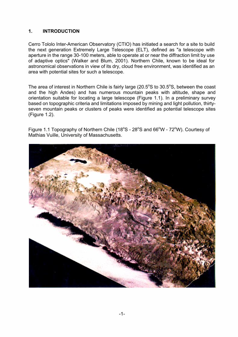
1. INTRODUCTION Cerro Tololo Inter-American Observatory (CTIO) has initiated a search for a site to build the next generation Extremely Large Telescope (ELT), defined as "a telescope with aperture in the range 30-100 meters, able to operate at or near the diffraction limit by use of adaptive optics" (Walker and Blum, 2001). Northern Chile, known to be ideal for astronomical observations in view of its dry, cloud free environment, was identified as an area with potential sites for such a telescope. The area of interest in Northern Chile is fairly large (20.5oS to 30.5oS, between the coast and the high Andes) and has numerous mountain peaks with altitude, shape and orientation suitable for locating a large telescope (Figure 1.1). In a preliminary survey based on topographic criteria and limitations imposed by mining and light pollution, thirty-seven mountain peaks or clusters of peaks were identified as potential telescope sites (Figure 1.2). Figure 1.1 Topography of Northern Chile (18oS - 28oS and 66oW - 72oW). Courtesy of Mathias Vuille, University of Massachusetts.

-1-

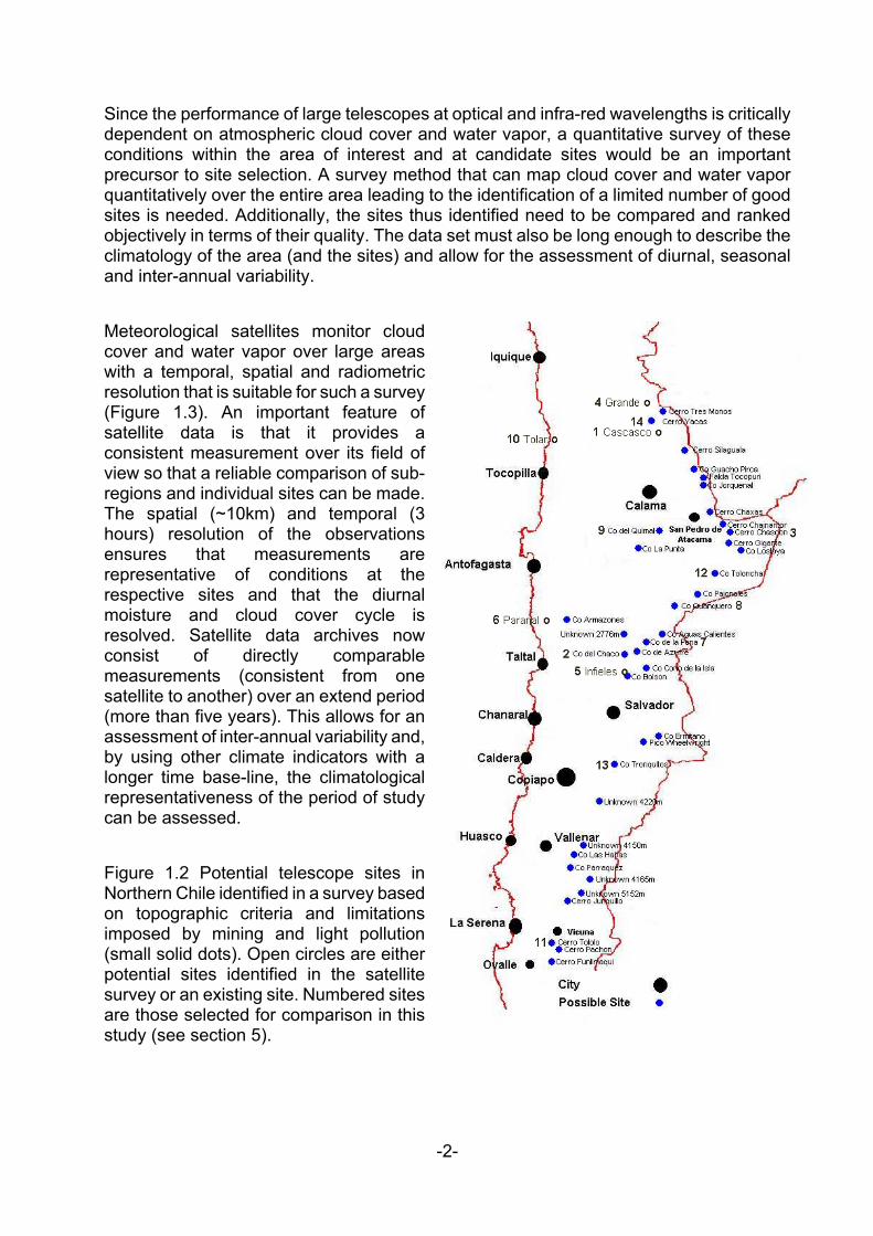
Since the performance of large telescopes at optical and infra-red wavelengths is critically dependent on atmospheric cloud cover and water vapor, a quantitative survey of these conditions within the area of interest and at candidate sites would be an important precursor to site selection. A survey method that can map cloud cover and water vapor quantitatively over the entire area leading to the identification of a limited number of good sites is needed. Additionally, the sites thus identified need to be compared and ranked objectively in terms of their quality. The data set must also be long enough to describe the climatology of the area (and the sites) and allow for the assessment of diurnal, seasonal and inter-annual variability. Meteorological satellites monitor cloud cover and water vapor over large areas with a temporal, spatial and radiometric resolution that is suitable for such a survey (Figure 1.3). An important feature of satellite data is that it provides a consistent measurement over its field of view so that a reliable comparison of sub-regions and individual sites can be made. The spatial (~10km) and temporal (3 hours) resolution of the observations ensures that measurements are representative of conditions at the respective sites and that the diurnal moisture and cloud cover cycle is resolved. Satellite data archives now consist of directly comparable measurements (consistent from one satellite to another) over an extend period (more than five years). This allows for an assessment of inter-annual variability and, by using other climate indicators with a longer time base-line, the climatological representativeness of the period of study can be assessed. Figure 1.2 Potential telescope sites in Northern Chile identified in a survey based on topographic criteria and limitations imposed by mining and light pollution (small solid dots). Open circles are either potential sites identified in the satellite survey or an existing site. Numbered sites are those selected for comparison in this study (see section 5).

-2-

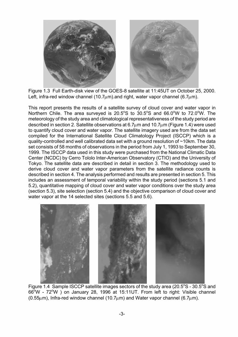
Figure 1.3 Full Earth-disk view of the GOES-8 satellite at 11:45UT on October 25, 2000. Left, infra-red window channel (10.7µm).and right, water vapor channel (6.7µm). This report presents the results of a satellite survey of cloud cover and water vapor in Northern Chile. The area surveyed is 20.5oS to 30.5oS and 66.0oW to 72.0oW. The meteorology of the study area and climatological representativeness of the study period are described in section 2. Satellite observations at 6.7µm and 10.7µm (Figure 1.4) were used to quantify cloud cover and water vapor. The satellite imagery used are from the data set compiled for the International Satellite Cloud Climatology Project (ISCCP) which is a quality-controlled and well calibrated data set with a ground resolution of ~10km. The data set consists of 58 months of observations in the period from July 1, 1993 to September 30, 1999. The ISCCP data used in this study were purchased from the National Climatic Data Center (NCDC) by Cerro Tololo Inter-American Observatory (CTIO) and the University of Tokyo. The satellite data are described in detail in section 3. The methodology used to derive cloud cover and water vapor parameters from the satellite radiance counts is described in section 4. The analysis performed and results are presented in section 5. This includes an assessment of temporal variability within the study period (sections 5.1 and 5.2), quantitative mapping of cloud cover and water vapor conditions over the study area (section 5.3), site selection (section 5.4) and the objective comparison of cloud cover and water vapor at the 14 selected sites (sections 5.5 and 5.6).

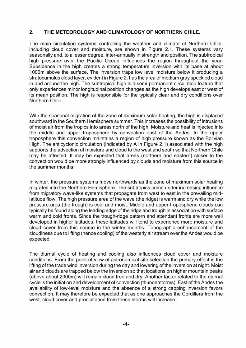
Figure 1.4 Sample ISCCP satellite images sectors of the study area (20.5oS - 30.5oS and 66oW - 72oW ) on January 28, 1996 at 15:11UT. From left to right: Visible channel (0.55µm), Infra-red window channel (10.7µm) and Water vapor channel (6.7µm).

-3-

2. THE METEOROLOGY AND CLIMATOLOGY OF NORTHERN CHILE. The main circulation systems controlling the weather and climate of Northern Chile, including cloud cover and moisture, are shown in Figure 2.1. These systems vary seasonally and, to a lesser degree, inter-annually in strength and position. The subtropical high pressure over the Pacific Ocean influences the region throughout the year. Subsidence in the high creates a strong temperature inversion with its base at about 1000m above the surface. The inversion traps low level moisture below it producing a stratocumulus cloud layer, evident in Figure 2.1 as the area of medium gray speckled cloud in and around the high. The subtropical high is a semi-permanent circulation feature that only experiences minor longitudinal position changes as the high develops east or west of its mean position. The high is responsible for the typically clear and dry conditions over Northern Chile. With the seasonal migration of the zone of maximum solar heating, the high is displaced southward in the Southern Hemisphere summer. This increases the possibility of intrusions of moist air from the tropics into areas north of the high. Moisture and heat is injected into the middle and upper troposphere by convection east of the Andes. In the upper troposphere this convection maintains a region of high pressure known as the Bolivian High. The anticyclonic circulation (indicated by A in Figure 2.1) associated with the high supports the advection of moisture and cloud to the west and south so that Northern Chile may be affected. It may be expected that areas (northern and eastern) closer to the convection would be more strongly influenced by clouds and moisture from this source in the summer months. In winter, the pressure systems move northwards as the zone of maximum solar heating migrates into the Northern Hemisphere. The subtropics come under increasing influence from migratory wave-like systems that propagate from west to east in the prevailing mid-latitude flow. The high pressure area of the wave (the ridge) is warm and dry while the low pressure area (the trough) is cool and moist. Middle and upper tropospheric clouds can typically be found along the leading edge of the ridge and trough in association with surface warm and cold fronts. Since the trough-ridge pattern and attendant fronts are more well developed in higher latitudes, these latitudes will tend to experience more moisture and cloud cover from this source in the winter months. Topographic enhancement of the cloudiness due to lifting (hence cooling) of the westerly air stream over the Andes would be expected. The diurnal cycle of heating and cooling also influences cloud cover and moisture conditions. From the point of view of astronomical site selection the primary effect is the lifting of the trade wind inversion during the day and lowering of the inversion at night. Moist air and clouds are trapped below the inversion so that locations on higher mountain peaks (above about 2000m) will remain cloud free and dry. Another factor related to the diurnal cycle is the initiation and development of convection (thunderstorms). East of the Andes the availability of low-level moisture and the absence of a strong capping inversion favors convection. It may therefore be expected that as one approaches the Cordillera from the west, cloud cover and precipitation from these storms will increase.

-4-

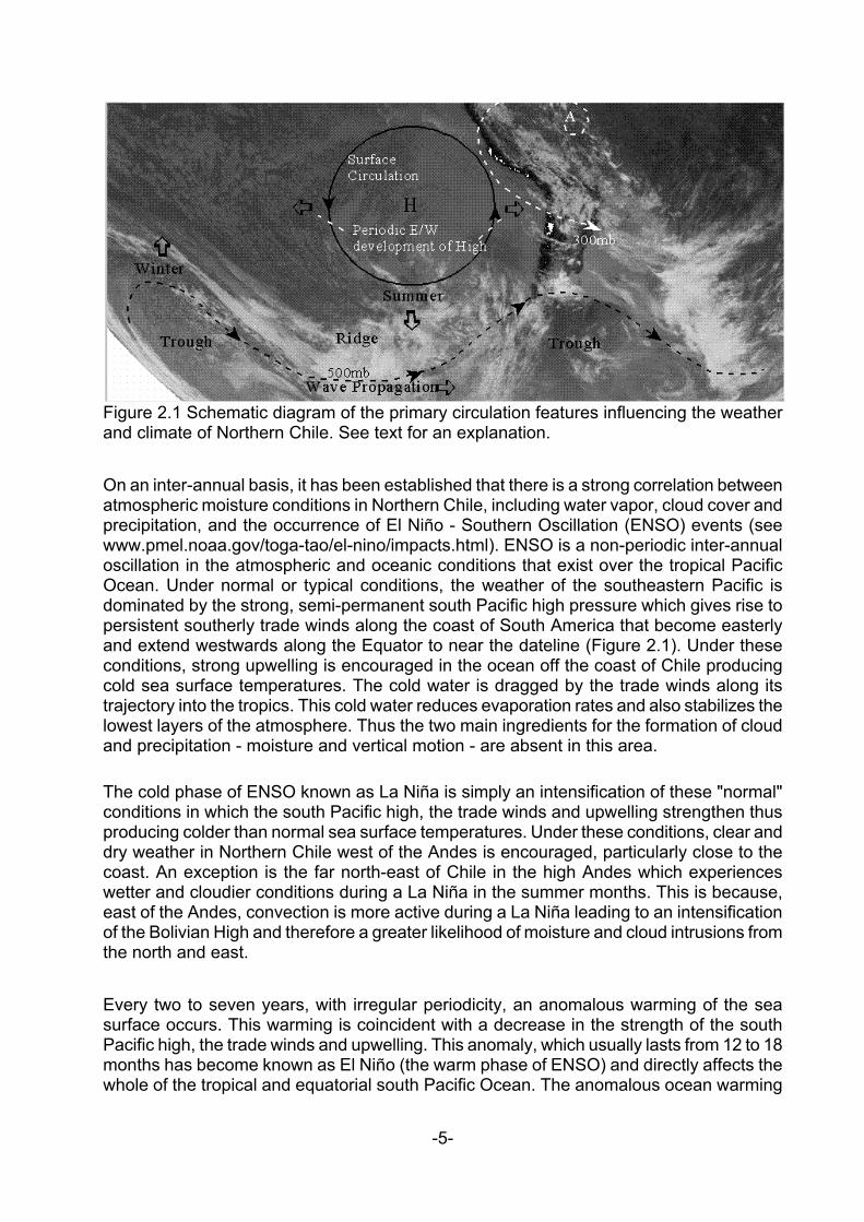
Figure 2.1 Schematic diagram of the primary circulation features influencing the weather and climate of Northern Chile. See text for an explanation. On an inter-annual basis, it has been established that there is a strong correlation between atmospheric moisture conditions in Northern Chile, including water vapor, cloud cover and precipitation, and the occurrence of El Niño - Southern Oscillation (ENSO) events (see www.pmel.noaa.gov/toga-tao/el-nino/impacts.html). ENSO is a non-periodic inter-annual oscillation in the atmospheric and oceanic conditions that exist over the tropical Pacific Ocean. Under normal or typical conditions, the weather of the southeastern Pacific is dominated by the strong, semi-permanent south Pacific high pressure which gives rise to persistent southerly trade winds along the coast of South America that become easterly and extend westwards along the Equator to near the dateline (Figure 2.1). Under these conditions, strong upwelling is encouraged in the ocean off the coast of Chile producing cold sea surface temperatures. The cold water is dragged by the trade winds along its trajectory into the tropics. This cold water reduces evaporation rates and also stabilizes the lowest layers of the atmosphere. Thus the two main ingredients for the formation of cloud and precipitation - moisture and vertical motion - are absent in this area. The cold phase of ENSO known as La Niña is simply an intensification of these "normal" conditions in which the south Pacific high, the trade winds and upwelling strengthen thus producing colder than normal sea surface temperatures. Under these conditions, clear and dry weather in Northern Chile west of the Andes is encouraged, particularly close to the coast. An exception is the far north-east of Chile in the high Andes which experiences wetter and cloudier conditions during a La Niña in the summer months. This is because, east of the Andes, convection is more active during a La Niña leading to an intensification of the Bolivian High and therefore a greater likelihood of moisture and cloud intrusions from the north and east. Every two to seven years, with irregular periodicity, an anomalous warming of the sea surface occurs. This warming is coincident with a decrease in the strength of the south Pacific high, the trade winds and upwelling. This anomaly, which usually lasts from 12 to 18 months has become known as El Niño (the warm phase of ENSO) and directly affects the whole of the tropical and equatorial south Pacific Ocean. The anomalous ocean warming

-5-

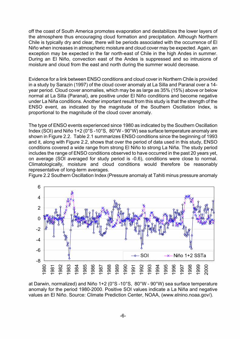
off the coast of South America promotes evaporation and destabilizes the lower layers of the atmosphere thus encouraging cloud formation and precipitation. Although Northern Chile is typically dry and clear, there will be periods associated with the occurrence of El Niño when increases in atmospheric moisture and cloud cover may be expected. Again, an exception may be expected in the far north-east of Chile in the high Andes in summer. During an El Niño, convection east of the Andes is suppressed and so intrusions of moisture and cloud from the east and north during the summer would decrease. Evidence for a link between ENSO conditions and cloud cover in Northern Chile is provided in a study by Sarazin (1997) of the cloud cover anomaly at La Silla and Paranal over a 14-year period. Cloud cover anomalies, which may be as large as 35% (15%) above or below normal at La Silla (Paranal), are positive under El Niño conditions and become negative under La Niña conditions. Another important result from this study is that the strength of the ENSO event, as indicated by the magnitude of the Southern Oscillation Index, is proportional to the magnitude of the cloud cover anomaly. The type of ENSO events experienced since 1980 as indicated by the Southern Oscillation Index (SOI) and Niño 1+2 (0°S -10°S, 80°W - 90°W) sea surface temperature anomaly are shown in Figure 2.2. Table 2.1 summarizes ENSO conditions since the beginning of 1993 and it, along with Figure 2.2, shows that over the period of data used in this study, ENSO conditions covered a wide range from strong El Niño to strong La Niña. The study period includes the range of ENSO conditions observed to have occurred in the past 20 years yet, on average (SOI averaged for study period is -0.6), conditions were close to normal. Climatologically, moisture and cloud conditions would therefore be reasonably representative of long-term averages. Figure 2.2 Southern Oscillation Index (Pressure anomaly at Tahiti minus pressure anomaly

at Darwin, normalized) and Niño 1+2 (0°S -10°S, 80°W - 90°W) sea surface temperature anomaly for the period 1980-2000. Positive SOI values indicate a La Niña and negative values an El Niño. Source: Climate Prediction Center, NOAA, (www.elnino.noaa.gov/).

-8

-6

-4

-2

0

2

4

6

1980

1981

1982

1983

1984

1985

1986

1987

1988

1989

1990

1991

1992

1993

1994

1995

1996

1997

1998

1999

2000

SOI Niño 1+2 SSTa

-6-

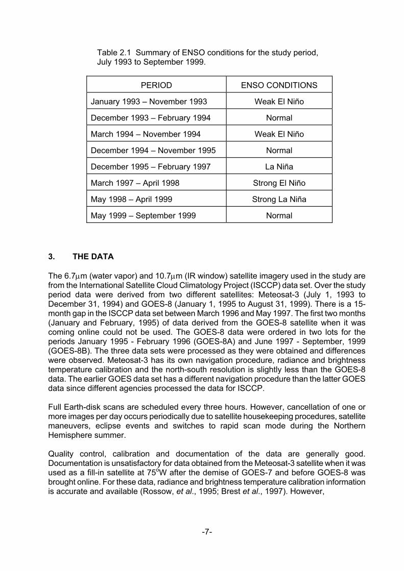
Table 2.1 Summary of ENSO conditions for the study period, July 1993 to September 1999.

PERIOD

ENSO CONDITIONS January 1993 – November 1993

Weak El Niño

December 1993 – February 1994

Normal

March 1994 – November 1994

Weak El Niño

December 1994 – November 1995

Normal

December 1995 – February 1997

La Niña

March 1997 – April 1998

Strong El Niño

May 1998 – April 1999

Strong La Niña

May 1999 – September 1999

Normal

3. THE DATA The 6.7µm (water vapor) and 10.7µm (IR window) satellite imagery used in the study are from the International Satellite Cloud Climatology Project (ISCCP) data set. Over the study period data were derived from two different satellites: Meteosat-3 (July 1, 1993 to December 31, 1994) and GOES-8 (January 1, 1995 to August 31, 1999). There is a 15-month gap in the ISCCP data set between March 1996 and May 1997. The first two months (January and February, 1995) of data derived from the GOES-8 satellite when it was coming online could not be used. The GOES-8 data were ordered in two lots for the periods January 1995 - February 1996 (GOES-8A) and June 1997 - September, 1999 (GOES-8B). The three data sets were processed as they were obtained and differences were observed. Meteosat-3 has its own navigation procedure, radiance and brightness temperature calibration and the north-south resolution is slightly less than the GOES-8 data. The earlier GOES data set has a different navigation procedure than the latter GOES data since different agencies processed the data for ISCCP. Full Earth-disk scans are scheduled every three hours. However, cancellation of one or more images per day occurs periodically due to satellite housekeeping procedures, satellite maneuvers, eclipse events and switches to rapid scan mode during the Northern Hemisphere summer. Quality control, calibration and documentation of the data are generally good. Documentation is unsatisfactory for data obtained from the Meteosat-3 satellite when it was used as a fill-in satellite at 75oW after the demise of GOES-7 and before GOES-8 was brought online. For these data, radiance and brightness temperature calibration information is accurate and available (Rossow, et al., 1995; Brest et al., 1997). However,

-7-

a suitable calibration of the upper tropospheric humidity (UTH), a derived water vapor parameter, was not carried out. Since the satellite was on loan from EUMETSAT to NOAA during this period, EUMETSAT did not consider the UTH calibration to be their responsibility. For NOAA, their focus at the time was on GOES-8 consequently no calibration was done for the conversion of Meteosat-3 water vapor brightness temperatures to UTH. Efforts were made, unsuccessfully, to obtain UTH calibration information for Meteosat-3. It was decided to obtain a period of overlapping satellite data for Meteosat-3 and GOES-8 so that an inter-calibration could be performed. (An accurate UTH calibration is available for GOES-8 data.) Repeated problems were encountered in attempts to obtain such an overlapping data set. In view of these developments a calibration of UTH for Meteosat-3 was undertaken using the daily Denver rawinsonde data for 1994. The calibration produced through this effort has enabled a seamless transition from the Meteosat-3 data to the GOES-8 data. More information on the calibration can be found in Appendix A and the successful merging of the two data sets is demonstrated in section 5.1. The data format of the ISCCP data (Campbell, et. al, 1997) is a mixture of McIdas (www.ssec.wisc.edu/software/mcidas.html) format and documentation data transmitted directly from the satellite. The basic structure of the data set is a header containing sector specifications, navigation constants and calibration coefficients. This is followed by scan lines of data from the multi-spectral imager interlaced by pixel. Each scan line is preceded by an 80 byte header which includes the time of the scan. The first part of the header provides information on the image sector data to follow such as the limits of the scan area, time of scan, channels included, spatial resolution and byte positions for the start of each data section. The next section of the header contains the parameters required for input to the software used to navigate the image areas. A program which converts pixel location to latitude-longitude position with an accuracy of 4km is provided by the National Environmental Satellite Data Information Service (NESDIS). The calibration section of the header provides the data needed to convert the radiance counts to true radiances. Meteosat and GOES perform real-time calibrations of infra-red detectors on-board the satellite using sensor readings from dark space and reference blackbodies. Calibration coefficients thus derived are used to compute radiance values from the raw counts. Further information on the computation of radiance values and derived parameters is given in section 4. Following the header are the data for the sector (in our case full-disk) arranged according to observation channel, viz. visible, infra-red window channel (10.7µm) and water vapor channel (6.7µm). The data are classified as B1 (highest spatial resolution) by ISCCP. Raw GOES-8 data are 1km resolution in the visible, 4x4km in the infra-red window channel and 4x8 km (effectively 8x8 km) in the water vapor channel. For ISCCP, the raw data are sampled so that the effective pixel resolution for all channels is 9.1 km x 8.0 km at Nadir. 4. METHODOLOGY

-8-

In this study, measurements of water vapor and cloud are derived from meteorological satellite observations by passive remote sensing at different wavelengths. The satellite measures the monochromatic emittance of the earth and atmosphere at 10.7µm in the infra-red window and at 6.7µm, a water vapor absorption band. Depending on the

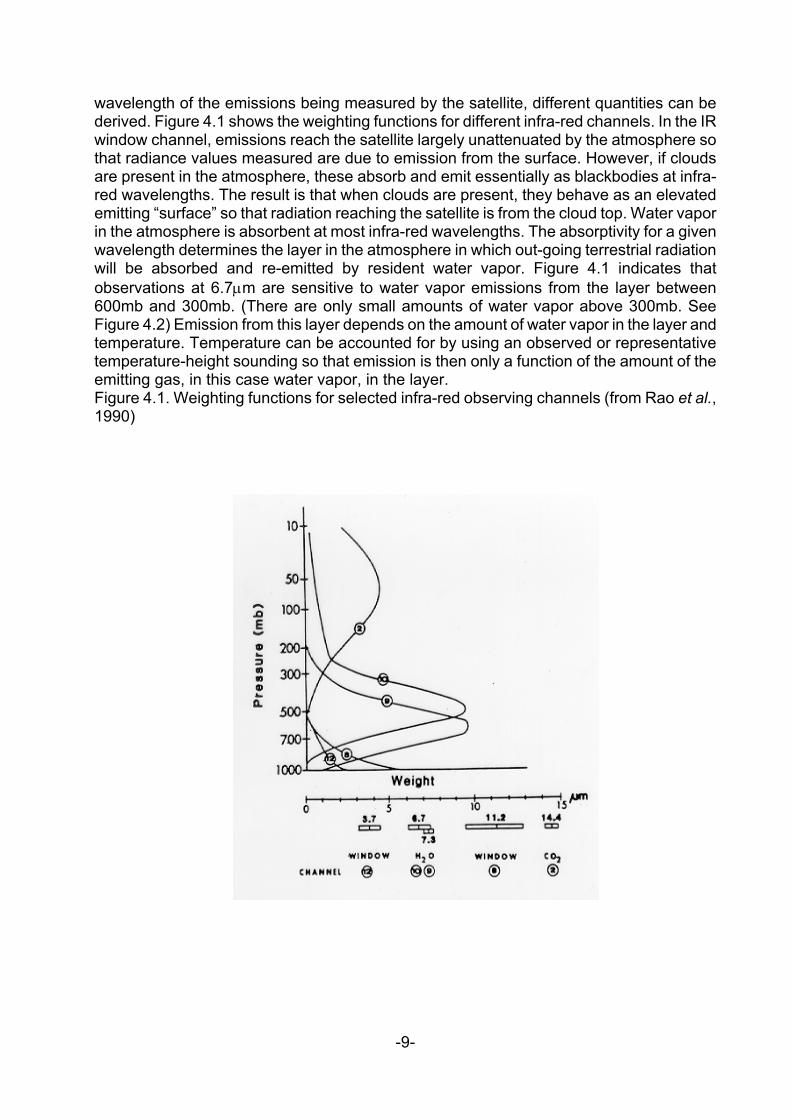
wavelength of the emissions being measured by the satellite, different quantities can be derived. Figure 4.1 shows the weighting functions for different infra-red channels. In the IR window channel, emissions reach the satellite largely unattenuated by the atmosphere so that radiance values measured are due to emission from the surface. However, if clouds are present in the atmosphere, these absorb and emit essentially as blackbodies at infra-red wavelengths. The result is that when clouds are present, they behave as an elevated emitting “surface” so that radiation reaching the satellite is from the cloud top. Water vapor in the atmosphere is absorbent at most infra-red wavelengths. The absorptivity for a given wavelength determines the layer in the atmosphere in which out-going terrestrial radiation will be absorbed and re-emitted by resident water vapor. Figure 4.1 indicates that observations at 6.7µm are sensitive to water vapor emissions from the layer between 600mb and 300mb. (There are only small amounts of water vapor above 300mb. See Figure 4.2) Emission from this layer depends on the amount of water vapor in the layer and temperature. Temperature can be accounted for by using an observed or representative temperature-height sounding so that emission is then only a function of the amount of the emitting gas, in this case water vapor, in the layer. Figure 4.1. Weighting functions for selected infra-red observing channels (from Rao et al., 1990)

-9-

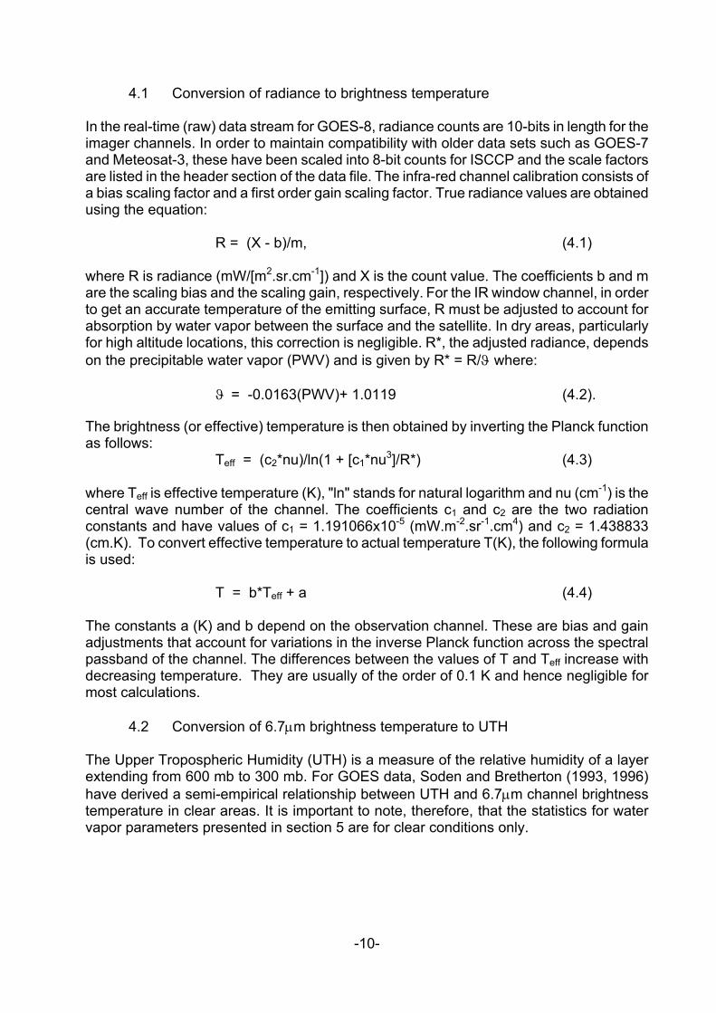
4.1 Conversion of radiance to brightness temperature In the real-time (raw) data stream for GOES-8, radiance counts are 10-bits in length for the imager channels. In order to maintain compatibility with older data sets such as GOES-7 and Meteosat-3, these have been scaled into 8-bit counts for ISCCP and the scale factors are listed in the header section of the data file. The infra-red channel calibration consists of a bias scaling factor and a first order gain scaling factor. True radiance values are obtained using the equation:

R = (X - b)/m, (4.1) where R is radiance (mW/[m2.sr.cm-1]) and X is the count value. The coefficients b and m are the scaling bias and the scaling gain, respectively. For the IR window channel, in order to get an accurate temperature of the emitting surface, R must be adjusted to account for absorption by water vapor between the surface and the satellite. In dry areas, particularly for high altitude locations, this correction is negligible. R*, the adjusted radiance, depends on the precipitable water vapor (PWV) and is given by R* = R/ϑ where: ϑ = -0.0163(PWV)+ 1.0119 (4.2). The brightness (or effective) temperature is then obtained by inverting the Planck function as follows:

Teff = (c2*nu)/ln(1 + [c1*nu3]/R*) (4.3) where Teff is effective temperature (K), "ln" stands for natural logarithm and nu (cm-1) is the central wave number of the channel. The coefficients c1 and c2 are the two radiation constants and have values of c1 = 1.191066x10-5 (mW.m-2.sr-1.cm4) and c2 = 1.438833 (cm.K). To convert effective temperature to actual temperature T(K), the following formula is used:

T = b*Teff + a (4.4)

The constants a (K) and b depend on the observation channel. These are bias and gain adjustments that account for variations in the inverse Planck function across the spectral passband of the channel. The differences between the values of T and Teff increase with decreasing temperature. They are usually of the order of 0.1 K and hence negligible for most calculations.

4.2 Conversion of 6.7µm brightness temperature to UTH The Upper Tropospheric Humidity (UTH) is a measure of the relative humidity of a layer extending from 600 mb to 300 mb. For GOES data, Soden and Bretherton (1993, 1996) have derived a semi-empirical relationship between UTH and 6.7µm channel brightness temperature in clear areas. It is important to note, therefore, that the statistics for water vapor parameters presented in section 5 are for clear conditions only.

-10-

The basic form of the relationship is:

UTH = [exp(a + b*T) * Cos θ] / p0 (4.5), where θ is the satellite viewing zenith angle, a and b are the least squares fit slope and intercept of the regression line as defined by the empirical relationship and p0 is a normalized pressure variable.

p0 = p(T=240K)/ 300, (4.6) where p (in mb) is the pressure level where the temperature (T) is 240K. The values for a and b are seasonally dependent and are obtained from a table listing their values for each month of the year. Since no suitable UTH calibration was available for the ISCCP data from Meteosat-3, a special calibration was done for the purposes of this study using the Denver rawinsonde data for 1994 (see Appendix A).

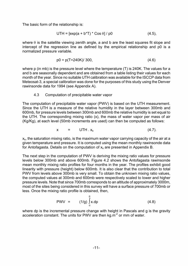
4.3 Computation of precipitable water vapor The computation of precipitable water vapor (PWV) is based on the UTH measurement. Since the UTH is a measure of the relative humidity in the layer between 300mb and 600mb, for pressure levels between 300mb and 600mb the relative humidity is set equal to the UTH. The corresponding mixing ratio (x), the mass of water vapor per mass of air (Kg/Kg), at each level (50mb increments are used) can then be computed as follows:

x = UTH . xs (4.7). xs, the saturation mixing ratio, is the maximum water vapor carrying capacity of the air at a given temperature and pressure. It is computed using the mean monthly rawinsonde data for Antofagasta. Details on the computation of xs are presented in Appendix B. The next step in the computation of PWV is deriving the mixing ratio values for pressure levels below 300mb and above 600mb. Figure 4.2 shows the Antofagasta rawinsonde mean monthly mixing ratio profiles for four months in the year. The profiles exhibit good linearity with pressure (height) below 600mb. It is also clear that the contribution to total PWV from levels above 300mb is very small. To obtain the unknown mixing ratio values, the computed values at 300mb and 600mb were respectively scaled to lower and higher pressure levels. Note that since 700mb corresponds to an altitude of approximately 3000m, most of the sites being considered in this survey will have a surface pressure of 700mb or less. Once the mixing ratio profile is obtained, then, p

PWV = (1/g) ∫ x.dp (4.8) o

where dp is the incremental pressure change with height in Pascals and g is the gravity acceleration constant. The units for PWV are then kg.m-2 or mm of water.

-11-

0

5

10

15

20

25

30

35

100200300400500600700800Pressure (mb)

Wat

er V

apor

Mixi

ng R

atio

(g/K

g)*1

0 Jan 12UTApr 12UTJuly 12UTOct 12UT

Figure 4.2 Mean monthly water vapor mixing ratio versus pressure (height) profiles as determined from the Antofagasta rawinsonde for the 10 year period 1977-1986. Cold surfaces at high altitude have an impact on the computation of PWV. The effect is limited to sites with an altitude above the 600mb (~4400m) pressure level under very dry conditions at night. These locations are affected because, at 6.7µm, the satellite senses emissions from the layer between 600mb and 300mb. Therefore, if the surface extends above the 600mb level, emission from the surface may be measured. This only occurs under very dry conditions (PWV <~ 1 mm) when there is insufficient moisture in the air above the surface to absorb all emissions from the surface. An example is shown in Figure 4.3.

Figure 4.3 Water vapor channel images for June 3-4, 1998 showing the effect of cold surfaces at high altitude under very dry conditions. Note how the high altitude areas around the Salar de Atacama that are dark (dry) in the daytime image appear light (relatively moist) in the nighttime image.

-12-

05:45UT

17:45UT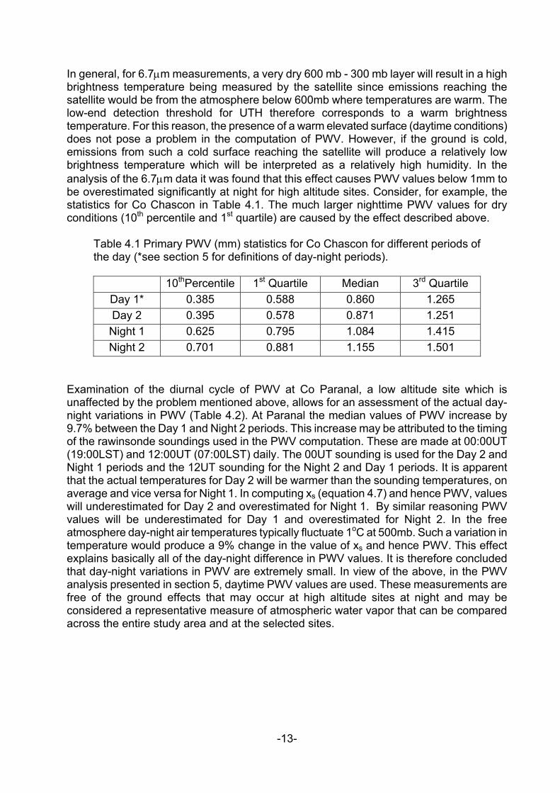

In general, for 6.7µm measurements, a very dry 600 mb - 300 mb layer will result in a high brightness temperature being measured by the satellite since emissions reaching the satellite would be from the atmosphere below 600mb where temperatures are warm. The low-end detection threshold for UTH therefore corresponds to a warm brightness temperature. For this reason, the presence of a warm elevated surface (daytime conditions) does not pose a problem in the computation of PWV. However, if the ground is cold, emissions from such a cold surface reaching the satellite will produce a relatively low brightness temperature which will be interpreted as a relatively high humidity. In the analysis of the 6.7µm data it was found that this effect causes PWV values below 1mm to be overestimated significantly at night for high altitude sites. Consider, for example, the statistics for Co Chascon in Table 4.1. The much larger nighttime PWV values for dry conditions (10th percentile and 1st quartile) are caused by the effect described above.

Table 4.1 Primary PWV (mm) statistics for Co Chascon for different periods of the day (*see section 5 for definitions of day-night periods).

10thPercentile 1st Quartile Median 3rd Quartile

Day 1* 0.385 0.588 0.860 1.265 Day 2 0.395 0.578 0.871 1.251

Night 1 0.625 0.795 1.084 1.415 Night 2 0.701 0.881 1.155 1.501

Examination of the diurnal cycle of PWV at Co Paranal, a low altitude site which is unaffected by the problem mentioned above, allows for an assessment of the actual day-night variations in PWV (Table 4.2). At Paranal the median values of PWV increase by 9.7% between the Day 1 and Night 2 periods. This increase may be attributed to the timing of the rawinsonde soundings used in the PWV computation. These are made at 00:00UT (19:00LST) and 12:00UT (07:00LST) daily. The 00UT sounding is used for the Day 2 and Night 1 periods and the 12UT sounding for the Night 2 and Day 1 periods. It is apparent that the actual temperatures for Day 2 will be warmer than the sounding temperatures, on average and vice versa for Night 1. In computing xs (equation 4.7) and hence PWV, values will underestimated for Day 2 and overestimated for Night 1. By similar reasoning PWV values will be underestimated for Day 1 and overestimated for Night 2. In the free atmosphere day-night air temperatures typically fluctuate 1oC at 500mb. Such a variation in temperature would produce a 9% change in the value of xs and hence PWV. This effect explains basically all of the day-night difference in PWV values. It is therefore concluded that day-night variations in PWV are extremely small. In view of the above, in the PWV analysis presented in section 5, daytime PWV values are used. These measurements are free of the ground effects that may occur at high altitude sites at night and may be considered a representative measure of atmospheric water vapor that can be compared across the entire study area and at the selected sites.

-13-

Table 4.2 Primary PWV (mm) statistics for Paranal for different periods of the day (*see section 5 for definitions of day-night periods).

Period 10th Percentile 1st Quartile Median 3rd Quartile Day 1* 1.781 2.640 3.994 5.860 Day 2 1.836 2.653 4.069 5.924 Night 1 1.969 2.877 4.427 6.255 Night 2 2.098 3.016 4.385 6.315

In order to further demonstrate the validity and representativeness of PWV measurements derived from the satellite, statistics were compared with those obtained from independent ground-based sensors. PWV measurements made from the ground at Paranal using a dark sky emissivity meter (www.eso.org/gen-fac/pubs/astclim) and at Chajnantor using a 183 GHz radiometer (alma.sc.eso.org) were obtained and primary statistics computed for test periods that overlap with the satellite data. Table 4.3 shows the primary PWV statistics for Paranal (January - August, 1998) and Chajnantor (January - September, 1999) as computed from the satellite data and from ground-based PWV sensors located at these sites.

Table 4.3 PWV (mm) statistics for Paranal (January - August 1998) and Chajnantor (January - September 1999) for satellite and ground-based site monitor measurements of PWV.

Site Paranal Chajnantor Sensor Satellite Site Monitor Satellite Site Monitor Period Day Night Day 24 hrs 10th percentile 1.83 1.70 0.30 0.26 1st Quartile 2.57 2.41 0.47 0.40 Median 4.05 3.66 0.72 0.77 3rd Quartile 7.27 5.21 1.26 2.16

The table shows that the satellite and ground-based monitor PWV statistics are generally in good agreement. Since an averaged rawinsonde temperature measurement is used in the satellite-derived PWV computation, there is a slight tendency for the satellite to overestimate PWV under very dry conditions and underestimate PWV under very moist conditions. This tendency is evident in the data for Chajnantor. At Paranal this is also occurring under dry conditions but under moist conditions an overriding factor causes PWV to be overestimated. For lower altitude sites, the extrapolation of the 600 mb mixing ratio down to the surface (~744 mb) becomes increasingly less valid as moisture levels increase (Erasmus and Maartens, 1999, 2001). In summary then, it has been shown that the satellite derived PWV for daytime hours gives a reliable and accurate absolute humidity measurement that is representative of daytime and nighttime moisture conditions.

-14-

4.4 Cloud detection and classification The presence of cirrus (high altitude) clouds and their thickness is inferred from the 6.7µm imagery. Since these clouds are found at an altitude (9-12km) higher than the water vapor emission layer, IR radiation from water vapor below the 300mb level is absorbed and re-emitted at colder temperatures by the cloud particles. Since the relationship between UTH and water vapor brightness temperature defined in section 4.2 is only valid under clear conditions, the presence of cirrus cloud particles causes UTH values to rise to the point that they are no longer valid. When UTH values rise to around 50%, cirrus cloud particles start forming by condensation and deposition (the cloud particles may not be visible at this stage). As UTH values rise further, the cloud particles grow in size and number and the cirrus cloud gets thicker. For pixels with UTH values above 50%, therefore, the UTH is an indicator of the presence and transparency of cirrus clouds. A first attempt at determining the threshold UTH values for the transition from clear to transparent and transparent to opaque conditions was made by visually comparing cirrus cloud in water vapor channel and IR window channel images (Erasmus and Peterson, 1996). Based on this comparison using Meteosat-3 data, threshold values of 72% and 150% were set. Subsequently, using better calibrated GOES-8 data, Erasmus and Sarazin (2000, 2001) have started to define these thresholds more accurately. They used atmospheric transparency measurements made on the ground at optical wavelengths and compared these to a transparency index based on the satellite UTH measurement. While this work is still in progress, Erasmus and Sarazin (2000, 2001) have shown that the satellite transparency index does effectively discriminate between photometric and non-photomeric observing conditions as measured by the Line Of Sight Sky Absorption Monitor (LOSSAM) at La Silla Observatory. The UTH threshold values have subsequently been revised as follows:

Clear: UTH ≤50% Opaque: UTH ≥100% Transparent: 50%<UTH<100%

The 10.7µm channel data are used to detect cloud in the middle and upper troposphere. In principle the procedure for cloud detection is straightforward. Pixel temperatures (Tir) computed from the 10.7µm satellite data need to be referenced against an independent temperature measurement. Typically, temperature drops with height in the atmosphere, so if Tir is colder (by some margin) than the surface temperature (for example) at a given pixel location, the presence of cloud above the surface is indicated. In practice, however, the task of unambiguous cloud detection presents several challenges. Firstly, for an area survey, an independent surface temperature observation for every pixel location is impossible. For the site comparison component of this study, surface temperature data are also largely non-existent. The most suitable reference measurement available in the study area is the Antofagasta (23.4oS, 70.4oW) rawinsonde. The next closest rawinsonde station to the study area is at Quintero (32.8oS, 71.5oW). Although this station is outside the area, it was used with the Antofagasta rawinsonde in the site comparison to derive an interpolated sounding for sites south of Antofagasta. Mean monthly rawinsonde data for the 00UT and 12UT soundings, based on a 10-year (1977-

-15-

1986) average, were obtained from the National Center for Atmospheric Research. The data are for pressure levels from the surface (~1000mb) to 200mb at 50mb increments (additional levels above 200mb are included but not used). Means and standard deviations of geopotential height, temperature, mixing ratio and component winds are provided for each level. How the rawinsonde temperatures are used to define the threshold temperature for cloud detection (Tr) is critical. As a first step towards determining Tr, the surface temperature (Ts) for a given pixel location may be estimated using the sounding data and digitized surface terrain heights. Given the altitude of the surface and the geopotential heights of the pressure levels, Ts can be estimated by interpolation from the rawinsonde data. The actual surface temperature may be warmer or colder than Ts. If it is warmer, this presents no problem for the detection of cloud since, if Tir < Ts , cloud is correctly determined to be present. However, if the actual temperature is colder than Ts and Tir < Ts then two conditions are possible - cloud may be present or the ground is incorrectly being interpreted as cloud. (Henceforth, this is referred to as "ground contamination".) Several different definitions for Tr were tested. For example, the rawinsonde data include the standard deviation of the temperature (σT) at each pressure level so that σT at the surface can be interpolated. Air temperature data are normally distributed so more than 99.74% of the time temperatures will be within 3σT of the mean. Thus an estimate can be made of the surface cold temperature extreme (Tr) as follows: Tr = Ts - 3σT. When Tr defined in this manner is used, ground contamination is still observed. This is the case since Ts is based on air temperatures as measured by the rawinsonde in the free air well above the surface. At an elevated surface location there may be additional cooling of the air by contact with the ground. This effect would be particularly noticeable in the early morning hours when radiative cooling of the surface is at a maximum. A secondary problem regarding unambiguous cloud detection relates to detecting cloud below 600mb over the ocean and along the coast. A temperature inversion commonly occurs between 900mb and 800mb (Figure 4.3). Over the ocean and along the coast, a cloud layer forms with its top at the base of the inversion. In Figure 4.3 it is apparent that the cloud top temperatures for cloud below the inversion is significantly colder (possibly as much as 10oC) than the air temperature at the inversion top (~800mb). Therefore, only at a pressure altitude of about 600mb do temperatures become colder than those observed at the inversion base. Therefore, if Tr is based on temperatures for pressure levels below 600mb and low cloud below the inversion exists, a pixel location would incorrectly be considered cloudy. This should be kept in mind when interpreting the maps that use the 700mb temperature as Tr.

400

500

600

700

800

900

1000-30 -20 -10 0 10 20 30

Temperature (oC)

Pres

sure

(mb)

Figure 4.3 Antofagasta rawinsonde temperature sounding on 4 July, 2000 at 12UT.

-16-

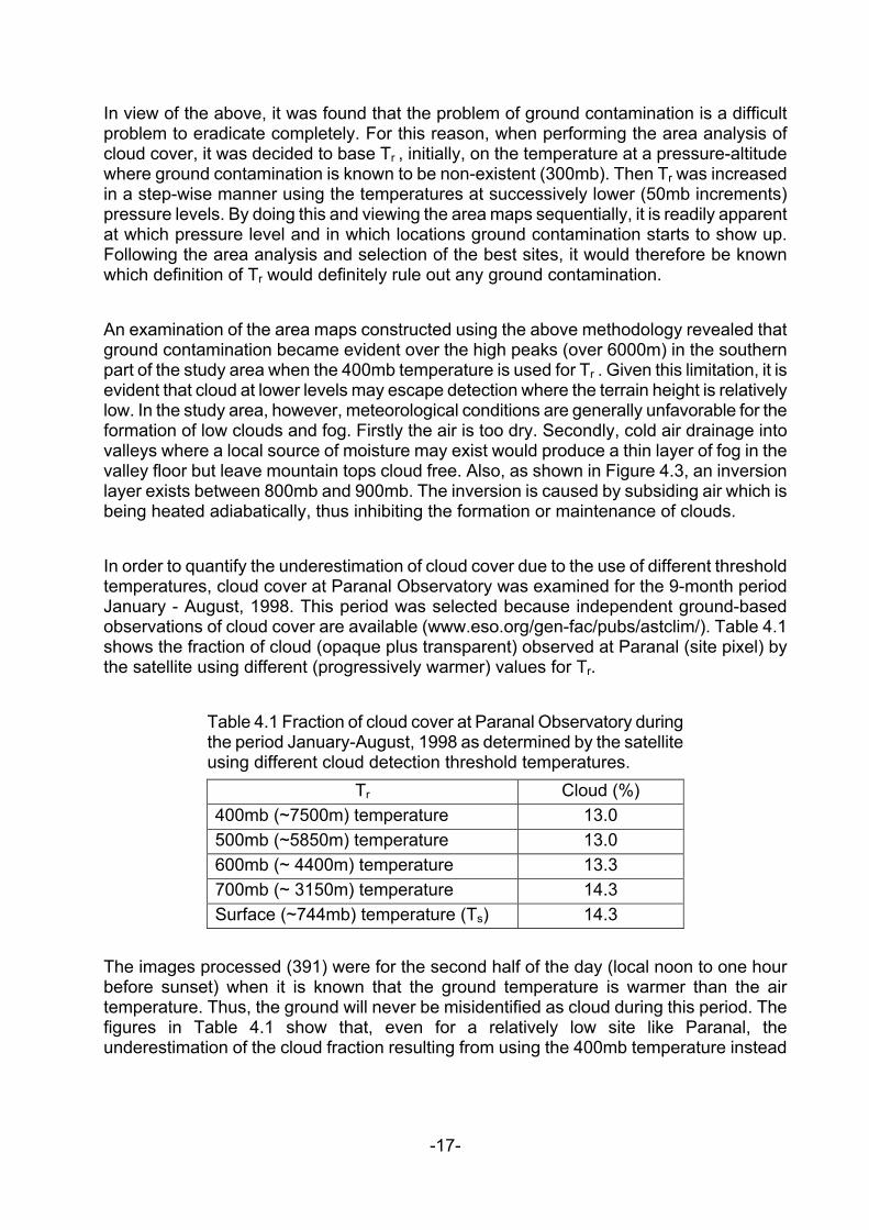
In view of the above, it was found that the problem of ground contamination is a difficult problem to eradicate completely. For this reason, when performing the area analysis of cloud cover, it was decided to base Tr , initially, on the temperature at a pressure-altitude where ground contamination is known to be non-existent (300mb). Then Tr was increased in a step-wise manner using the temperatures at successively lower (50mb increments) pressure levels. By doing this and viewing the area maps sequentially, it is readily apparent at which pressure level and in which locations ground contamination starts to show up. Following the area analysis and selection of the best sites, it would therefore be known which definition of Tr would definitely rule out any ground contamination. An examination of the area maps constructed using the above methodology revealed that ground contamination became evident over the high peaks (over 6000m) in the southern part of the study area when the 400mb temperature is used for Tr . Given this limitation, it is evident that cloud at lower levels may escape detection where the terrain height is relatively low. In the study area, however, meteorological conditions are generally unfavorable for the formation of low clouds and fog. Firstly the air is too dry. Secondly, cold air drainage into valleys where a local source of moisture may exist would produce a thin layer of fog in the valley floor but leave mountain tops cloud free. Also, as shown in Figure 4.3, an inversion layer exists between 800mb and 900mb. The inversion is caused by subsiding air which is being heated adiabatically, thus inhibiting the formation or maintenance of clouds. In order to quantify the underestimation of cloud cover due to the use of different threshold temperatures, cloud cover at Paranal Observatory was examined for the 9-month period January - August, 1998. This period was selected because independent ground-based observations of cloud cover are available (www.eso.org/gen-fac/pubs/astclim/). Table 4.1 shows the fraction of cloud (opaque plus transparent) observed at Paranal (site pixel) by the satellite using different (progressively warmer) values for Tr.

Table 4.1 Fraction of cloud cover at Paranal Observatory during the period January-August, 1998 as determined by the satellite using different cloud detection threshold temperatures.

Tr Cloud (%) 400mb (~7500m) temperature 13.0 500mb (~5850m) temperature 13.0 600mb (~ 4400m) temperature 13.3 700mb (~ 3150m) temperature 14.3 Surface (~744mb) temperature (Ts) 14.3

The images processed (391) were for the second half of the day (local noon to one hour before sunset) when it is known that the ground temperature is warmer than the air temperature. Thus, the ground will never be misidentified as cloud during this period. The figures in Table 4.1 show that, even for a relatively low site like Paranal, the underestimation of the cloud fraction resulting from using the 400mb temperature instead

-17-

of the surface temperature is only 1.3%. It should be noted that a large percentage of the sites selected for comparison in this study are higher than 4000m. The only exceptions are Co Paranal, Co Tololo and Tolar Tolar. Using the 400mb temperature for Tr and cloud cover categories defined below for the 9-pixel site area, a cloudy fraction of 17.1% was found for the observing night at Paranal in the period January - August, 1998. For the same period in 1998, cloud cover measurements made by a human observer during the observing night at Paranal indicate a cloudy fraction of 19.1%. Since 1.3% of this difference can be attributed to the definition of Tr, it can be seen that the satellite and ground observations are in good agreement. The other 0.7% difference between the satellite and ground observer measurement can not definitely be considered an additional underestimate on the part of the satellite. It is certainly possible that the latter difference may be due to the sampling methods used by the satellite and the ground observer. The ground observer measurement is an estimate of cloud cover looking upwards at two hour intervals during the observing night, starting at 00UT. The procedure for cloud detection in the analysis that follows uses observations made at both 6.7µm and 10.7µm. First, the 6.7µm imagery is used to determine the existence of transparent or opaque cirrus at high altitude. If a pixel is determined to have opaque cirrus then the final cloud cover classification for that pixel location is “opaque” since the corresponding pixel in the 10.7µm would also give an opaque signature. However, if a pixel is either clear or transparent from the 6.7µm image analysis, the corresponding pixel in the 10.7µm image is examined. If cloud is detected in that pixel then the pixel location is classified as opaque. If not, then pixel locations classified respectively as clear or transparent remain clear or transparent. The sky cover classifications described in the previous paragraph are the extent of those possible for individual pixels. The clear fraction, based on the classification described above, may be considered as an upper limit for the fraction of time that observing conditions are photometric. This is the case because:

(i) Sub-pixel scale cloud elements that are sufficiently small and/or sparse may lead to a pixel with such cloud elements being classified “clear”

(ii) A larger cloud element located partly in two or more pixels may result in the individual pixels being classified as clear if a sufficiently large fraction of the pixels are cloud free.

(iii) Pixels with UTH values near the Clear-Transparent threshold may not be purely photometric

A stricter and probably more accurate definition of clear (hence photometric) conditions can be attained by using a cluster of pixels to represent the site instead of an individual pixel. As shown schematically in Figure 4.4, a 9-pixel area may be used to represent the astronomical “sky” at the site. At the level of the Tropopause (about 12km), for an observer on the ground viewing the sky, this 9-pixel area would correspond to the sky within approximately 60o of zenith.

-18-

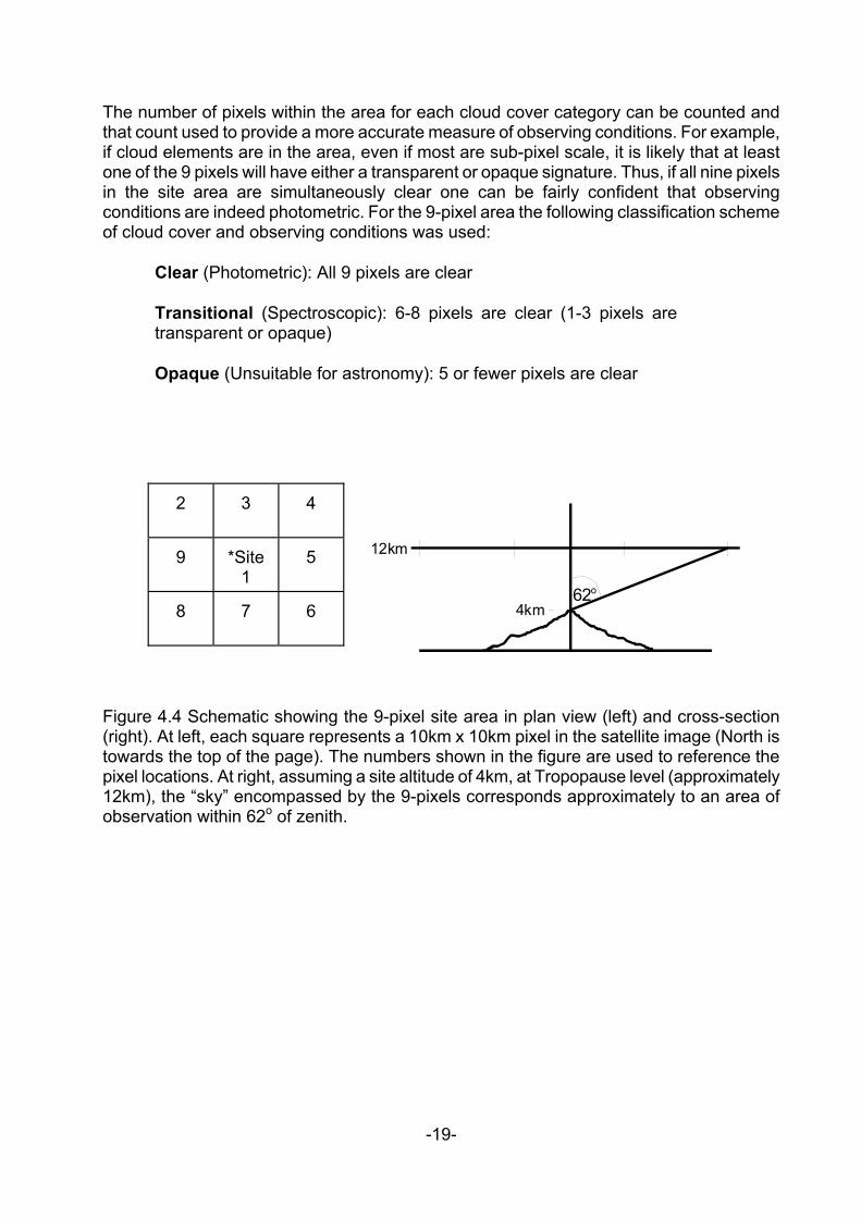
The number of pixels within the area for each cloud cover category can be counted and that count used to provide a more accurate measure of observing conditions. For example, if cloud elements are in the area, even if most are sub-pixel scale, it is likely that at least one of the 9 pixels will have either a transparent or opaque signature. Thus, if all nine pixels in the site area are simultaneously clear one can be fairly confident that observing conditions are indeed photometric. For the 9-pixel area the following classification scheme of cloud cover and observing conditions was used:

Clear (Photometric): All 9 pixels are clear Transitional (Spectroscopic): 6-8 pixels are clear (1-3 pixels are transparent or opaque)

Opaque (Unsuitable for astronomy): 5 or fewer pixels are clear

2

3

4

9

*Site

1

5

8

7

6

62o

4km

12km

Figure 4.4 Schematic showing the 9-pixel site area in plan view (left) and cross-section (right). At left, each square represents a 10km x 10km pixel in the satellite image (North is towards the top of the page). The numbers shown in the figure are used to reference the pixel locations. At right, assuming a site altitude of 4km, at Tropopause level (approximately 12km), the “sky” encompassed by the 9-pixels corresponds approximately to an area of observation within 62o of zenith.

-19-

5. ANALYSIS AND RESULTS Using the methodology described in section 4, cloud cover and water vapor conditions over the study area were quantified. Cloud cover maps showing either the clear, transitional or opaque fraction were constructed. Area maps for water vapor showing the percentage frequency of occurrence of PWV values below selected thresholds were plotted. Based on the area analysis the 10 best sites were identified. These, together with 4 other pre-selected sites, were analyzed and compared. With a few exceptions, the 10 best sites were drawn from a list of potential sites that met certain preconditions according to a topographical survey (www.ctio.noao.edu/sitetests/survey/scriteria.html). For the fourteen sites a detailed set of comparison statistics were derived. A complete set of maps and all statistical results from the analysis are provided on the attached CD. The cloud cover area maps were compiled using two methods. First, for each pixel location the cloud category was determined using the single pixel at that location. Second, for each pixel location the cloud cover category was derived from the 9-pixel area centered on that location. The latter method, of course, leaves one pixel along the perimeter unmapped. For PWV mapping, single pixel values were mapped. The frequency of occurrence of each PWV and cloud category was then counted for each pixel location, expressed as a percentage frequency and then contours were drawn. It was found, for cloud cover, that the two approaches yielded very similar cloud cover patterns with the 9-pixel area method providing a less noisy map. Since the purpose of the mapping is to define regional patterns leading to the identification of preferred areas, the cloud cover maps constructed using the 9-pixel area method were generally found to be more useful. Also, as noted in section 4, use of the 9-pixel cloud cover categories allows for a more accurate definition of astronomical observing conditions. The area maps were compiled for different periods of the day. Day-night divisions are based on the observing night (end twilight to start twilight) at Paranal Observatory. The length of the observing night for each season (defined below), is determined by the shortest night in each season. Daytime is the balance of the day less one hour each at the start and end of the daylight period. Nighttime and daytime periods thus defined are further divided in half giving four divisions: Day 1, Day 2, Night 1, Night 2. Since there are between 4 and 8 images per day it is impractical to divide the day into more than these four periods. In the detailed analysis of the sites, cloud cover and water vapor statistics are derived using the 9-pixel areas centered on each site location. Individual pixel values are used to evaluate cloud cover and water vapor variations within the site areas. Site comparison statistics were compiled for the entire data set, by season and for the four day-night divisions. Seasons are defined on a climatological basis as follows:

Summer - December, January, February (DJF) Fall - March, April, May (MAM) Winter - June, July, August (JJA)

Spring - September, October, November (SON) For the cloud cover analysis, the primary cloud cover indicators used are the percentage

-20-

frequency of clear (photometric), transitional (spectroscopic) or clear plus transitional (suitable for astronomy) conditions. Water vapor conditions are quantified in terms of the

-21-

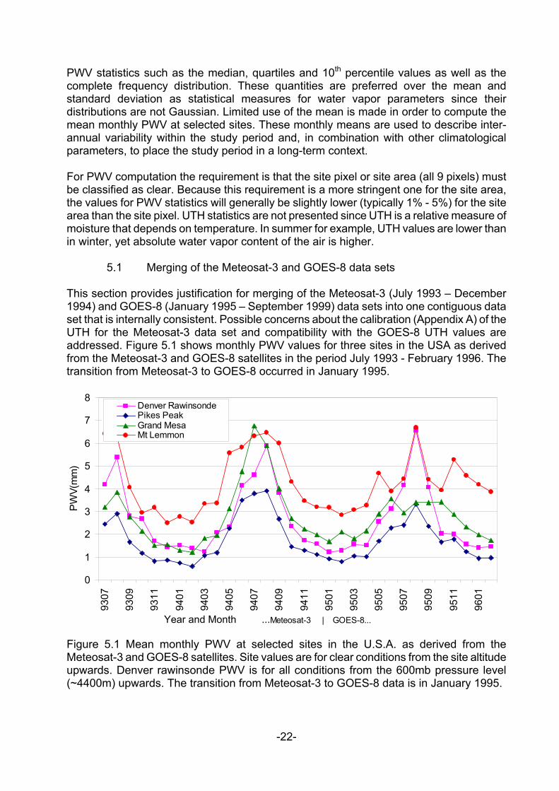
PWV statistics such as the median, quartiles and 10th percentile values as well as the complete frequency distribution. These quantities are preferred over the mean and standard deviation as statistical measures for water vapor parameters since their distributions are not Gaussian. Limited use of the mean is made in order to compute the mean monthly PWV at selected sites. These monthly means are used to describe inter-annual variability within the study period and, in combination with other climatological parameters, to place the study period in a long-term context. For PWV computation the requirement is that the site pixel or site area (all 9 pixels) must be classified as clear. Because this requirement is a more stringent one for the site area, the values for PWV statistics will generally be slightly lower (typically 1% - 5%) for the site area than the site pixel. UTH statistics are not presented since UTH is a relative measure of moisture that depends on temperature. In summer for example, UTH values are lower than in winter, yet absolute water vapor content of the air is higher. 5.1 Merging of the Meteosat-3 and GOES-8 data sets This section provides justification for merging of the Meteosat-3 (July 1993 – December 1994) and GOES-8 (January 1995 – September 1999) data sets into one contiguous data set that is internally consistent. Possible concerns about the calibration (Appendix A) of the UTH for the Meteosat-3 data set and compatibility with the GOES-8 UTH values are addressed. Figure 5.1 shows monthly PWV values for three sites in the USA as derived from the Meteosat-3 and GOES-8 satellites in the period July 1993 - February 1996. The transition from Meteosat-3 to GOES-8 occurred in January 1995.

0

1

2

3

4

5

6

7

8

9307

9309

9311

9401

9403

9405

9407

9409

9411

9501

9503

9505

9507

9509

9511

9601

Year and Month ...Meteosat-3 | GOES-8...

PW

V(m

m)

Denver RawinsondePikes PeakGrand MesaMt Lemmon

Figure 5.1 Mean monthly PWV at selected sites in the U.S.A. as derived from the Meteosat-3 and GOES-8 satellites. Site values are for clear conditions from the site altitude upwards. Denver rawinsonde PWV is for all conditions from the 600mb pressure level (~4400m) upwards. The transition from Meteosat-3 to GOES-8 data is in January 1995.

-22-

The PWV for the rawinsonde site is computed from the mean monthly profiles by integrating the mixing ratio values from the 600mb pressure level (~4400m) to the top of the troposphere. These values are therefore for all sky conditions – clear or cloudy. The PWV values for the sites are derived from the satellite as described in section 4 and therefore correspond to moisture above the sites. It is readily apparent that the UTH calibration performed for the Meteosat-3 data using the Denver rawinsonde provides for a smooth transition in moisture parameters across the time boundary of the two data sets. The three sites shown in Figure 5.1 are in geographically and climatologically diverse regions, yet at all the sites the transition between the data sets is seamless. In view of these findings the two data sets were merged and processed as one continuous data.

20

30

40

50

60

70

80

90

100

71993

11994

71994

11995

71995

11996

71996

11997

71997

11998

71998

11999

71999

Month and Year

% C

lear

Grande El Chaco Tololo

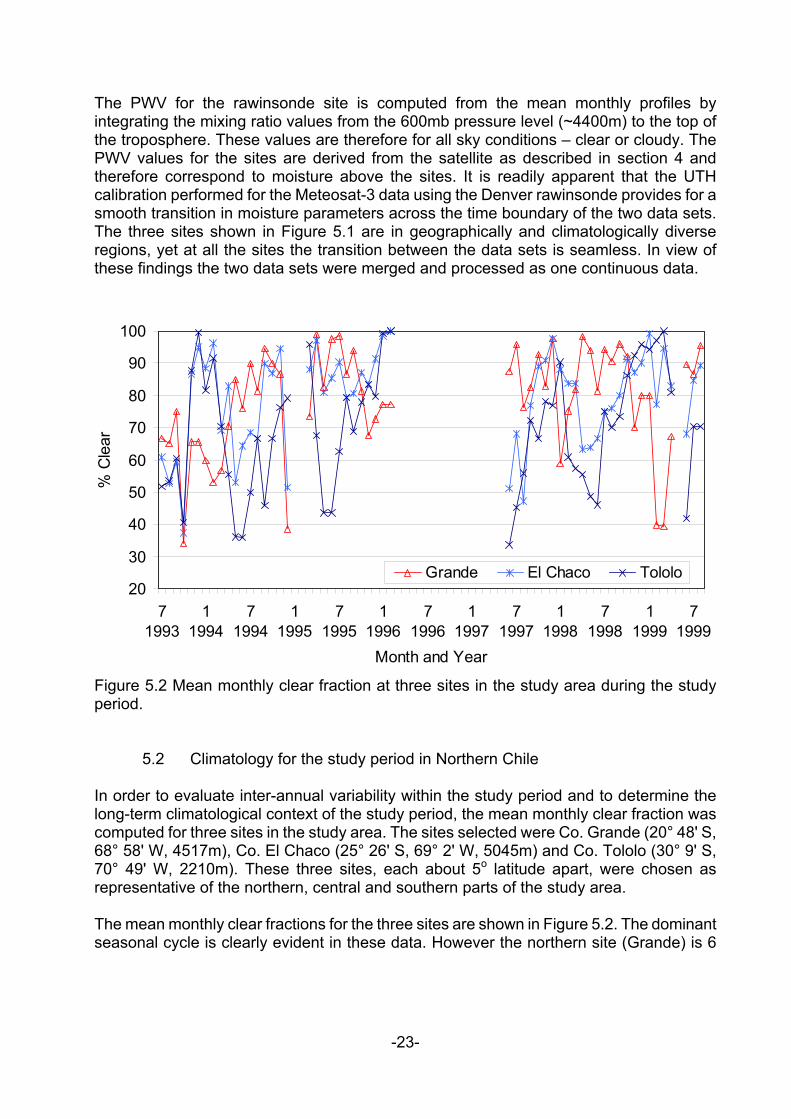
Figure 5.2 Mean monthly clear fraction at three sites in the study area during the study period. 5.2 Climatology for the study period in Northern Chile In order to evaluate inter-annual variability within the study period and to determine the long-term climatological context of the study period, the mean monthly clear fraction was computed for three sites in the study area. The sites selected were Co. Grande (20° 48' S, 68° 58' W, 4517m), Co. El Chaco (25° 26' S, 69° 2' W, 5045m) and Co. Tololo (30° 9' S, 70° 49' W, 2210m). These three sites, each about 5o latitude apart, were chosen as representative of the northern, central and southern parts of the study area. The mean monthly clear fractions for the three sites are shown in Figure 5.2. The dominant seasonal cycle is clearly evident in these data. However the northern site (Grande) is 6

-23-

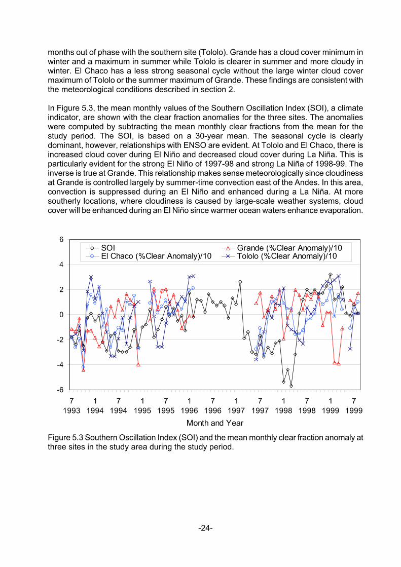
months out of phase with the southern site (Tololo). Grande has a cloud cover minimum in winter and a maximum in summer while Tololo is clearer in summer and more cloudy in winter. El Chaco has a less strong seasonal cycle without the large winter cloud cover maximum of Tololo or the summer maximum of Grande. These findings are consistent with the meteorological conditions described in section 2. In Figure 5.3, the mean monthly values of the Southern Oscillation Index (SOI), a climate indicator, are shown with the clear fraction anomalies for the three sites. The anomalies were computed by subtracting the mean monthly clear fractions from the mean for the study period. The SOI, is based on a 30-year mean. The seasonal cycle is clearly dominant, however, relationships with ENSO are evident. At Tololo and El Chaco, there is increased cloud cover during El Niño and decreased cloud cover during La Niña. This is particularly evident for the strong El Niño of 1997-98 and strong La Niña of 1998-99. The inverse is true at Grande. This relationship makes sense meteorologically since cloudiness at Grande is controlled largely by summer-time convection east of the Andes. In this area, convection is suppressed during an El Niño and enhanced during a La Niña. At more southerly locations, where cloudiness is caused by large-scale weather systems, cloud cover will be enhanced during an El Niño since warmer ocean waters enhance evaporation.

-6

-4

-2

0

2

4

6

71993

11994

71994

11995

71995

11996

71996

11997

71997

11998

71998

11999

71999

Month and Year

SOI Grande (%Clear Anomaly)/10El Chaco (%Clear Anomaly)/10 Tololo (%Clear Anomaly)/10

Figure 5.3 Southern Oscillation Index (SOI) and the mean monthly clear fraction anomaly at three sites in the study area during the study period.

-24-

5.3 Area analysis

Cloud cover maps show isolines of the percentage of clear skies, opaque cloud and transitional cloud cover respectively. PWV maps were plotted of the percentage frequency of occurrence of PWV observations below certain thresholds (0.5mm, 1.0mm, 2.0mm, 3.0mm). Each data set (Meteosat-3, GOES-8A and GOES-8B) was processed separately and then combined. Area maps were constructed for the four day-night divisions and using different definitions for Tr. In total, over 300 maps were produced. Since it is impractical to reproduce even a fraction of these maps in this report, a full set of maps is supplied on the attached CD. To show the primary features of the aerial distribution of cloud and PWV in this report, maps showing average conditions for the whole study period were constructed. As explained in section 4, in the construction of the area maps, successively warmer (lower pressure level) temperatures were used as the threshold for the detection of clouds in the infra-red window channel. The likelihood of interpreting a cold elevated surface under clear conditions as cloud increases as the threshold becomes warmer. This problem is most severe in the early morning hours. Figure 5.4 (a) - (c) shows the clear fraction for the observing night using the temperature at 300mb, 400mb and 500mb respectively as the threshold for cloud detection. It is evident that the ground detection problem starts to become manifest over the highest peaks (over 6000m) south of about 27oS when the 400mb temperature is used as a threshold. However, it is particularly noteworthy that when successively warmer thresholds are used, the isolines over the lower terrain do not change. This supports the finding made earlier for Paranal and described in section 4, that use of the 400mb temperature as the threshold for cloud detection does not lead to a significant underestimation of cloud cover. The clear, opaque and transitional fraction for the observing night over the entire study period is shown in Figure 5.5 (a) - (c). Over the study area the general pattern of cloud cover is for cloudiness to increase towards the east and south. The latitudinal minimum is between 21.5oS and 24.5oS. The north-south extent of the clearest zone decreases as one moves eastwards from the coast. At 69oW the minimum is at 23oS. Between 22oS and 24oS the largest west-east gradient in cloud cover occurs between 68oW and 69oW. The transitional cloud cover (partly cloudy and/or transparent cirrus) map shows that these conditions occur between 3% and 12% of the time. The map shows (erroneous) values above 12% where ground contamination is a problem (peaks over 6000m, south of 27oS). As may be expected, the transitional fraction increases with overall cloudiness. The diurnal cycle of the clear fraction is shown in Figures 5.6 (a) - (d). Morning hours are clearest. Dramatic increases in cloud cover are observed in the afternoon east of the Andes in association with the development of convective storms in this area. The impact of increased afternoon cloudiness extends west of the Cordillera due to local convection and the movement of cloud from the east under certain meteorological conditions. After sunset, clearing is observed east of the Andes as the convection subsides. However, west of about 68oW clearing during the night is gradual and slight. This suggests that the diurnal cycle of cloud cover in this area is controlled mostly by the movement of cloud produced to the east of the Andes into the region rather than local convection.

-25-

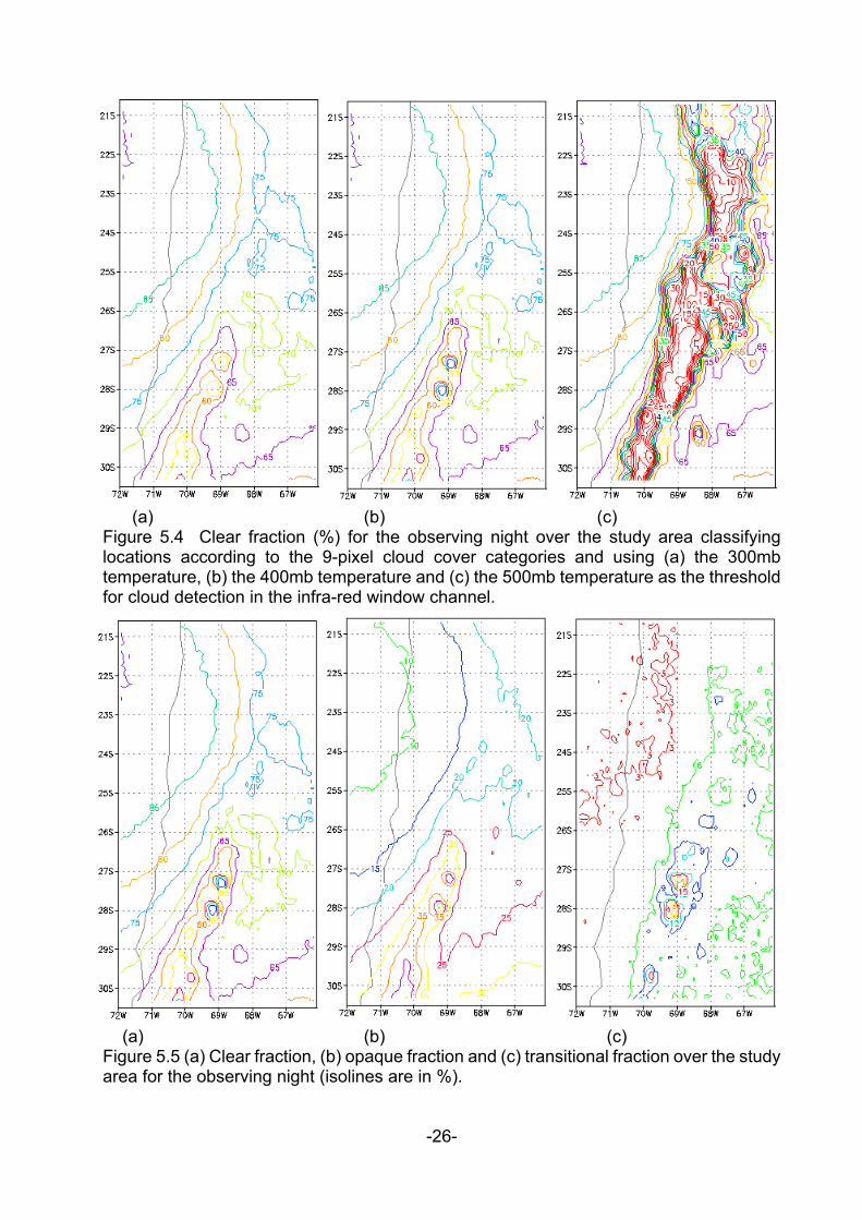
(a) (b) (c) Figure 5.4 Clear fraction (%) for the observing night over the study area classifying locations according to the 9-pixel cloud cover categories and using (a) the 300mb temperature, (b) the 400mb temperature and (c) the 500mb temperature as the threshold for cloud detection in the infra-red window channel.

(a) (b) (c) Figure 5.5 (a) Clear fraction, (b) opaque fraction and (c) transitional fraction over the study area for the observing night (isolines are in %).

-26-

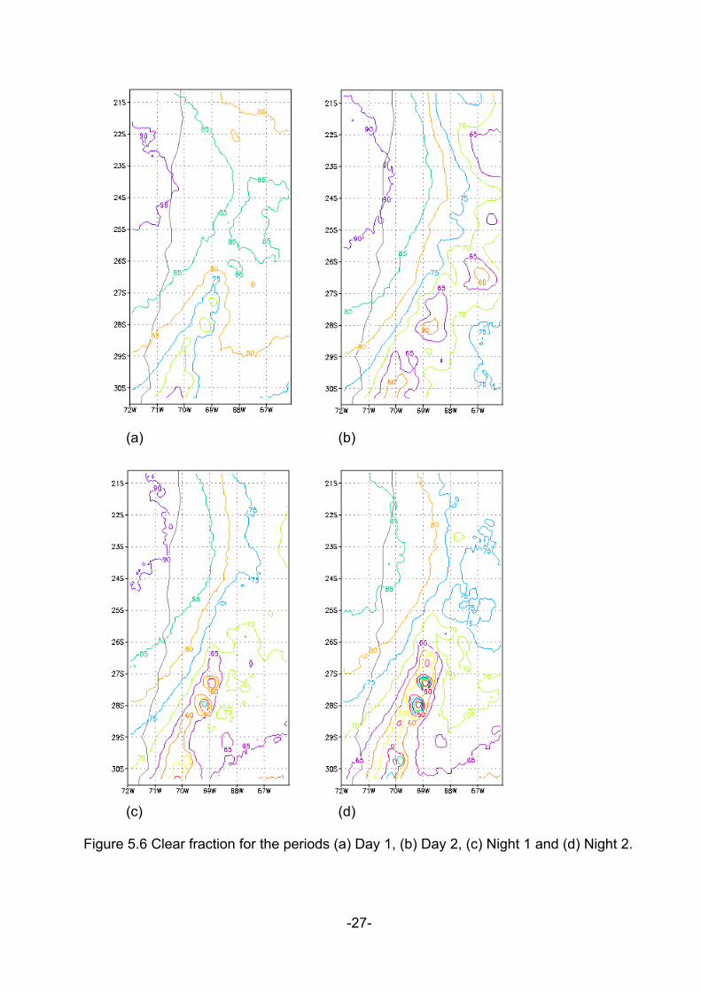
(a) (b) (c) (d) Figure 5.6 Clear fraction for the periods (a) Day 1, (b) Day 2, (c) Night 1 and (d) Night 2.

-27-

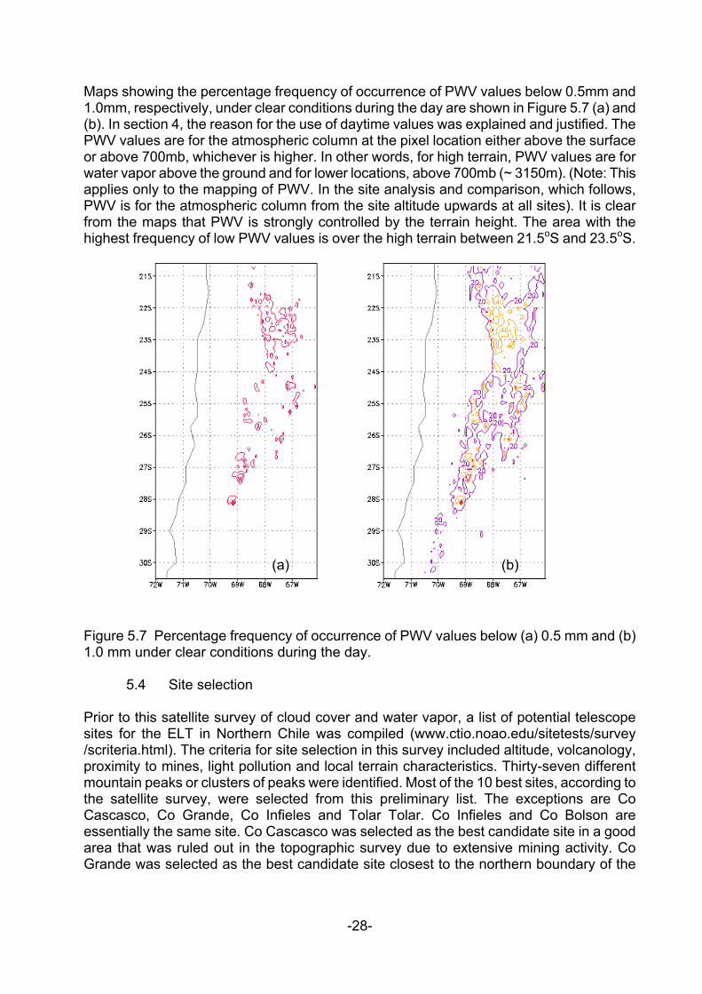
Maps showing the percentage frequency of occurrence of PWV values below 0.5mm and 1.0mm, respectively, under clear conditions during the day are shown in Figure 5.7 (a) and (b). In section 4, the reason for the use of daytime values was explained and justified. The PWV values are for the atmospheric column at the pixel location either above the surface or above 700mb, whichever is higher. In other words, for high terrain, PWV values are for water vapor above the ground and for lower locations, above 700mb (~ 3150m). (Note: This applies only to the mapping of PWV. In the site analysis and comparison, which follows, PWV is for the atmospheric column from the site altitude upwards at all sites). It is clear from the maps that PWV is strongly controlled by the terrain height. The area with the highest frequency of low PWV values is over the high terrain between 21.5oS and 23.5oS.

)

Figure 5.7 Percentage frequency of occurrence of PWV values be1.0 mm under clear conditions during the day. 5.4 Site selection Prior to this satellite survey of cloud cover and water vapor, a listsites for the ELT in Northern Chile was compiled (www.ctio.noa/scriteria.html). The criteria for site selection in this survey includedproximity to mines, light pollution and local terrain characteristicsmountain peaks or clusters of peaks were identified. Most of the 10 the satellite survey, were selected from this preliminary list. ThCascasco, Co Grande, Co Infieles and Tolar Tolar. Co Infieleessentially the same site. Co Cascasco was selected as the best carea that was ruled out in the topographic survey due to extensGrande was selected as the best candidate site closest to the no

-28-

(b)

(a

low (a) 0.5 mm and (b)

of potential telescope o.edu/sitetests/survey altitude, volcanology,

. Thirty-seven different best sites, according to e exceptions are Co

s and Co Bolson are andidate site in a good ive mining activity. Co rthern boundary of the

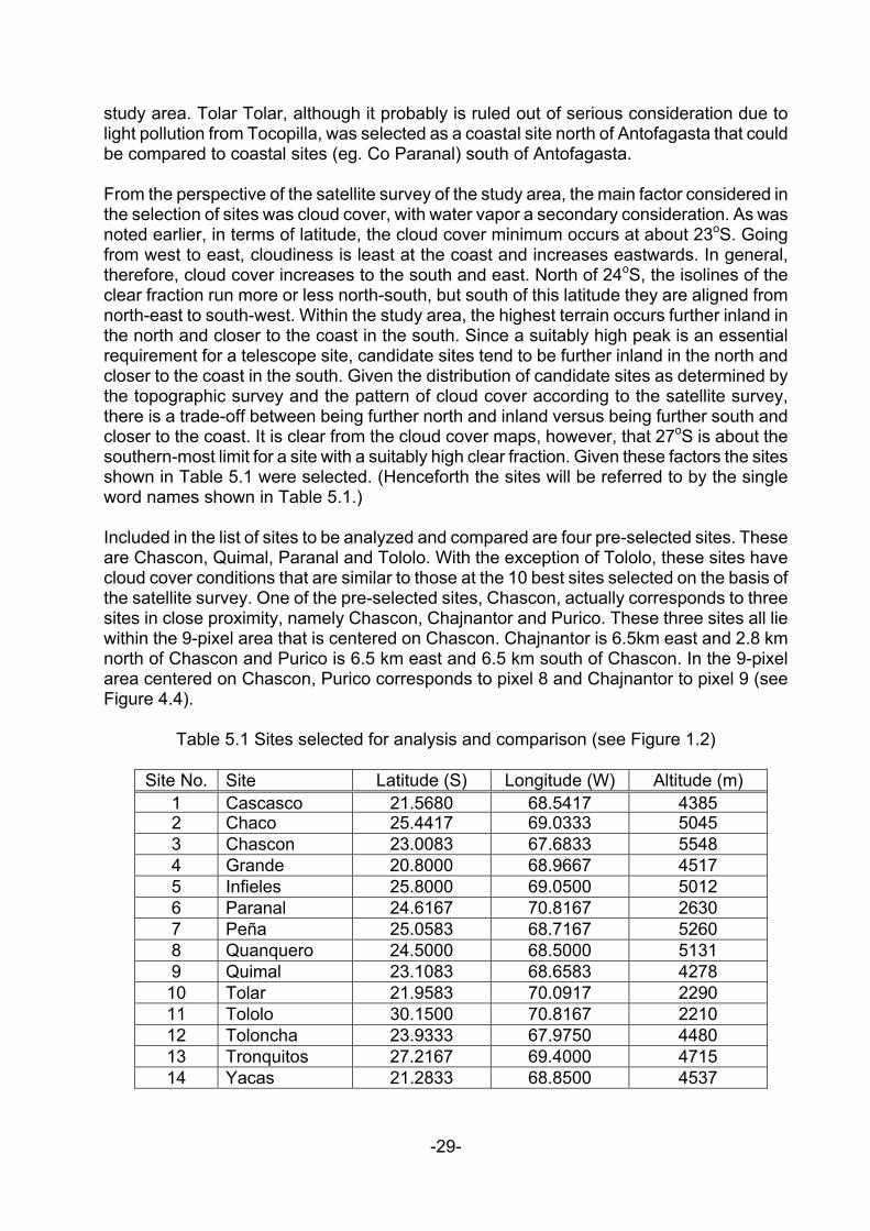
study area. Tolar Tolar, although it probably is ruled out of serious consideration due to light pollution from Tocopilla, was selected as a coastal site north of Antofagasta that could be compared to coastal sites (eg. Co Paranal) south of Antofagasta. From the perspective of the satellite survey of the study area, the main factor considered in the selection of sites was cloud cover, with water vapor a secondary consideration. As was noted earlier, in terms of latitude, the cloud cover minimum occurs at about 23oS. Going from west to east, cloudiness is least at the coast and increases eastwards. In general, therefore, cloud cover increases to the south and east. North of 24oS, the isolines of the clear fraction run more or less north-south, but south of this latitude they are aligned from north-east to south-west. Within the study area, the highest terrain occurs further inland in the north and closer to the coast in the south. Since a suitably high peak is an essential requirement for a telescope site, candidate sites tend to be further inland in the north and closer to the coast in the south. Given the distribution of candidate sites as determined by the topographic survey and the pattern of cloud cover according to the satellite survey, there is a trade-off between being further north and inland versus being further south and closer to the coast. It is clear from the cloud cover maps, however, that 27oS is about the southern-most limit for a site with a suitably high clear fraction. Given these factors the sites shown in Table 5.1 were selected. (Henceforth the sites will be referred to by the single word names shown in Table 5.1.) Included in the list of sites to be analyzed and compared are four pre-selected sites. These are Chascon, Quimal, Paranal and Tololo. With the exception of Tololo, these sites have cloud cover conditions that are similar to those at the 10 best sites selected on the basis of the satellite survey. One of the pre-selected sites, Chascon, actually corresponds to three sites in close proximity, namely Chascon, Chajnantor and Purico. These three sites all lie within the 9-pixel area that is centered on Chascon. Chajnantor is 6.5km east and 2.8 km north of Chascon and Purico is 6.5 km east and 6.5 km south of Chascon. In the 9-pixel area centered on Chascon, Purico corresponds to pixel 8 and Chajnantor to pixel 9 (see Figure 4.4).

Table 5.1 Sites selected for analysis and comparison (see Figure 1.2)

Site No. Site Latitude (S) Longitude (W) Altitude (m) 1 Cascasco 21.5680 68.5417 4385 2 Chaco 25.4417 69.0333 5045 3 Chascon 23.0083 67.6833 5548 4 Grande 20.8000 68.9667 4517 5 Infieles 25.8000 69.0500 5012 6 Paranal 24.6167 70.8167 2630 7 Peña 25.0583 68.7167 5260 8 Quanquero 24.5000 68.5000 5131 9 Quimal 23.1083 68.6583 4278

10 Tolar 21.9583 70.0917 2290 11 Tololo 30.1500 70.8167 2210 12 Toloncha 23.9333 67.9750 4480 13 Tronquitos 27.2167 69.4000 4715 14 Yacas 21.2833 68.8500 4537

-29-

5.5 Site Analysis: Cloud cover

5.5.1 Overall conditions

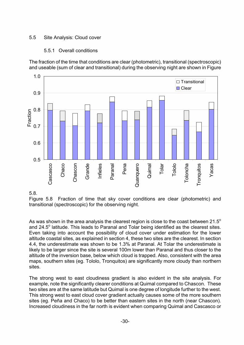
The fraction of the time that conditions are clear (photometric), transitional (spectroscopic) and useable (sum of clear and transitional) during the observing night are shown in Figure

5.8.

0.5

0.6

0.7

0.8

0.9

1.0

Cas

casc

o

Cha

co

Cha

scon

Gra

nde

Infie

les

Para

nal

Pena

Qua

nque

ro

Qui

mal

Tola

r

Tolo

lo

Tolo

ncha

Tron

quito

s

Yac

as

Frac

tion

TransitionalClear

Figure 5.8 Fraction of time that sky cover conditions are clear (photometric) and transitional (spectroscopic) for the observing night. As was shown in the area analysis the clearest region is close to the coast between 21.5o and 24.5o latitude. This leads to Paranal and Tolar being identified as the clearest sites. Even taking into account the possibility of cloud cover under estimation for the lower altitude coastal sites, as explained in section 4, these two sites are the clearest. In section 4.4, the underestimate was shown to be 1.3% at Paranal. At Tolar the underestimate is likely to be larger since the site is several 100m lower than Paranal and thus closer to the altitude of the inversion base, below which cloud is trapped. Also, consistent with the area maps, southern sites (eg. Tololo, Tronquitos) are significantly more cloudy than northern sites. The strong west to east cloudiness gradient is also evident in the site analysis. For example, note the significantly clearer conditions at Quimal compared to Chascon. These two sites are at the same latitude but Quimal is one degree of longitude further to the west. This strong west to east cloud cover gradient actually causes some of the more southern sites (eg. Peña and Chaco) to be better than eastern sites in the north (near Chascon). Increased cloudiness in the far north is evident when comparing Quimal and Cascasco or

-30-

Quimal and Yacas. These three sites are at about the same longitude but Cascasco and Yacas are further north. Quimal, Yacas and Cascasco are the three best inland sites.

-31-

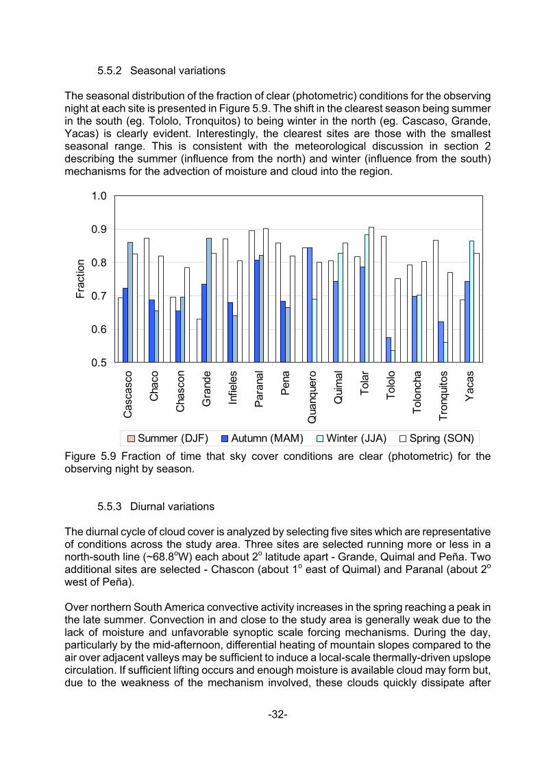
5.5.2 Seasonal variations The seasonal distribution of the fraction of clear (photometric) conditions for the observing night at each site is presented in Figure 5.9. The shift in the clearest season being summer in the south (eg. Tololo, Tronquitos) to being winter in the north (eg. Cascaso, Grande, Yacas) is clearly evident. Interestingly, the clearest sites are those with the smallest seasonal range. This is consistent with the meteorological discussion in section 2 describing the summer (influence from the north) and winter (influence from the south) mechanisms for the advection of moisture and cloud into the region.

0.5

0.6

0.7

0.8

0.9

1.0

Cas

casc

o

Cha

co

Cha

scon

Gra

nde

Infie

les

Para

nal

Pena

Qua

nque

ro

Qui

mal

Tola

r

Tolo

lo

Tolo

ncha

Tron

quito

s

Yac

as

Frac

tion

Summer (DJF) Autumn (MAM) Winter (JJA) Spring (SON)Figure 5.9 Fraction of time that sky cover conditions are clear (photometric) for the observing night by season. 5.5.3 Diurnal variations The diurnal cycle of cloud cover is analyzed by selecting five sites which are representative of conditions across the study area. Three sites are selected running more or less in a north-south line (~68.8oW) each about 2o latitude apart - Grande, Quimal and Peña. Two additional sites are selected - Chascon (about 1o east of Quimal) and Paranal (about 2o west of Peña). Over northern South America convective activity increases in the spring reaching a peak in the late summer. Convection in and close to the study area is generally weak due to the lack of moisture and unfavorable synoptic scale forcing mechanisms. During the day, particularly by the mid-afternoon, differential heating of mountain slopes compared to the air over adjacent valleys may be sufficient to induce a local-scale thermally-driven upslope circulation. If sufficient lifting occurs and enough moisture is available cloud may form but, due to the weakness of the mechanism involved, these clouds quickly dissipate after

-32-

sunset.

-33-

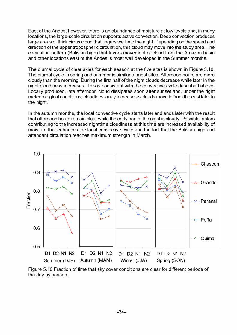
East of the Andes, however, there is an abundance of moisture at low levels and, in many locations, the large-scale circulation supports active convection. Deep convection produces large areas of thick cirrus cloud that lingers well into the night. Depending on the speed and direction of the upper tropospheric circulation, this cloud may move into the study area. The circulation pattern (Bolivian high) that favors movement of cloud from the Amazon basin and other locations east of the Andes is most well developed in the Summer months. The diurnal cycle of clear skies for each season at the five sites is shown in Figure 5.10. The diurnal cycle in spring and summer is similar at most sites. Afternoon hours are more cloudy than the morning. During the first half of the night clouds decrease while later in the night cloudiness increases. This is consistent with the convective cycle described above. Locally produced, late afternoon cloud dissipates soon after sunset and, under the right meteorological conditions, cloudiness may increase as clouds move in from the east later in the night. In the autumn months, the local convective cycle starts later and ends later with the result that afternoon hours remain clear while the early part of the night is cloudy. Possible factors contributing to the increased nighttime cloudiness at this time are increased availability of moisture that enhances the local convective cycle and the fact that the Bolivian high and attendant circulation reaches maximum strength in March.

D1 D2 N1 N2Autumn (MAM)

0.5

0.6

0.7

0.8

0.9

1.0

D1 D2 N1 N2Summer (DJF)

Frac

tion

D1 D2 N1 N2Winter (JJA)

D1 D2 N1 N2Spring (SON)

Chascon

Grande

Paranal

Peña

Quimal

Figure 5.10 Fraction of time that sky cover conditions are clear for different periods of the day by season.

-34-

In the winter, diurnal cloud cover variations are unrelated to convection. The sites away from the high Andes have small variations in cloud cover through the day which is consistent with the fact that cloud cover at this time of the year is generally due to large scale weather systems that do not have a preferred time of occurrence during the day. The two sites (Chascon and Peña) in (or closer to) the high Andes are cloudier and show a noticeable increase in cloudiness during the night. This is no doubt due to lifting of the westerly air stream over the Cordillera forming orographic cloud. This cloud is stratiform in nature. During the night, the tops of stratiform cloud layers cool radiatively. This destabilizes the layer, enhancing vertical motion within the layer, cooling and cloud particle formation. 5.5.4 Local spatial variations Variations in cloud cover within the 9-pixel area centered on each site are considered in this section. Local topography may have an effect on where convective clouds develop and this may lead to noticeable variations in cloud cover within the 9-pixel area. For the observing night, at each station the difference between the clear fraction at each pixel surrounding the site and the center pixel was computed. The results are presented in Table 5.2. In general, clear fraction variations within the 9-pixel are small, typically 1-4% across the 9-pixel areas. The maximum difference at any site between the site pixel and an adjacent pixel was found to be 2.1%. The maximum difference between any two pixels was 4.2%. Both of these extremes were observed at Tronquitos. At most sites, cloud cover increases from north-west to south-east across the 9-pixel areas. This is consistent with the general pattern of cloudiness across the study area. A notable exception is Chascon where the local cloud cover increases from east to west. The maximum difference (2%) is observed between pixels 6 and 8 (south-east corner to south-west corner). This increase in cloudiness is clearly due to the influence of the Salar de Atacama which is a moisture source. Locally produced convective clouds increase cloud cover directly east of the Salar and south-west of Chascon. An example of an event producing cloud in this manner is shown in Figure 5.11. The two additional pre-selected sites near Chascon, namely, Purico and Chajnantor correspond to pixel numbers 8 and 9 respectively. At these locations the clear fraction is about 1% lower than at Chascon.

-35-

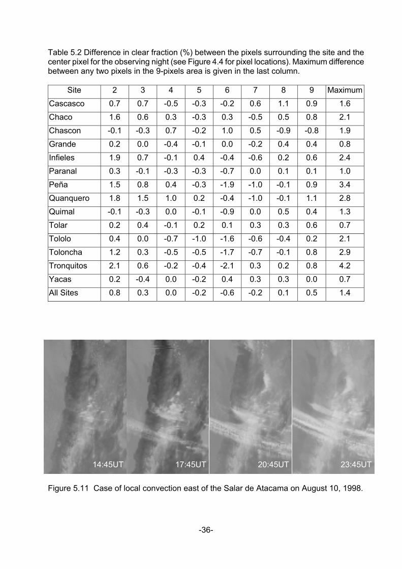
Table 5.2 Difference in clear fraction (%) between the pixels surrounding the site and the center pixel for the observing night (see Figure 4.4 for pixel locations). Maximum difference between any two pixels in the 9-pixels area is given in the last column.

Site 2 3 4 5 6 7 8 9 Maximum

Cascasco 0.7 0.7 -0.5 -0.3 -0.2 0.6 1.1 0.9 1.6

Chaco 1.6 0.6 0.3 -0.3 0.3 -0.5 0.5 0.8 2.1

Chascon -0.1 -0.3 0.7 -0.2 1.0 0.5 -0.9 -0.8 1.9

Grande 0.2 0.0 -0.4 -0.1 0.0 -0.2 0.4 0.4 0.8

Infieles 1.9 0.7 -0.1 0.4 -0.4 -0.6 0.2 0.6 2.4

Paranal 0.3 -0.1 -0.3 -0.3 -0.7 0.0 0.1 0.1 1.0

Peña 1.5 0.8 0.4 -0.3 -1.9 -1.0 -0.1 0.9 3.4

Quanquero 1.8 1.5 1.0 0.2 -0.4 -1.0 -0.1 1.1 2.8

Quimal -0.1 -0.3 0.0 -0.1 -0.9 0.0 0.5 0.4 1.3

Tolar 0.2 0.4 -0.1 0.2 0.1 0.3 0.3 0.6 0.7

Tololo 0.4 0.0 -0.7 -1.0 -1.6 -0.6 -0.4 0.2 2.1

Toloncha 1.2 0.3 -0.5 -0.5 -1.7 -0.7 -0.1 0.8 2.9

Tronquitos 2.1 0.6 -0.2 -0.4 -2.1 0.3 0.2 0.8 4.2

Yacas 0.2 -0.4 0.0 -0.2 0.4 0.3 0.3 0.0 0.7

All Sites 0.8 0.3 0.0 -0.2 -0.6 -0.2 0.1 0.5 1.4

Figure 5.11

14:45UT

Case of local convect

17:45UT

ion east of the Salar d

-36-

e

20:45UT

Atacama on August 10

23:45UT

, 1998.

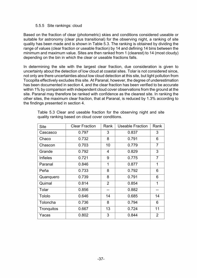
5.5.5 Site rankings: cloud Based on the fraction of clear (photometric) skies and conditions considered useable or suitable for astronomy (clear plus transitional) for the observing night, a ranking of site quality has been made and is shown in Table 5.3. The ranking is obtained by dividing the range of values (clear fraction or useable fraction) by 14 and defining 14 bins between the minimum and maximum value. Sites are then ranked from 1 (clearest) to 14 (most cloudy) depending on the bin in which the clear or useable fractions falls. In determining the site with the largest clear fraction, due consideration is given to uncertainty about the detection of low cloud at coastal sites. Tolar is not considered since, not only are there uncertainties about low cloud detection at this site, but light pollution from Tocopilla effectively excludes this site. At Paranal, however, the degree of underestimation has been documented in section 4, and the clear fraction has been verified to be accurate within 1% by comparison with independent cloud cover observations from the ground at the site. Paranal may therefore be ranked with confidence as the clearest site. In ranking the other sites, the maximum clear fraction, that at Paranal, is reduced by 1.3% according to the findings presented in section 4.

Table 5.3 Clear and useable fraction for the observing night and site quality ranking based on cloud cover conditions.

Site Clear Fraction Rank Useable Fraction Rank Cascasco 0.797 3 0.837 3 Chaco 0.732 8 0.791 6 Chascon 0.703 10 0.779 7 Grande 0.792 4 0.829 3 Infieles 0.721 9 0.775 7 Paranal 0.846 1 0.877 1 Peña 0.733 8 0.792 6 Quanquero 0.739 8 0.791 6 Quimal 0.814 2 0.854 1 Tolar 0.856 -- 0.882 -- Tololo 0.646 14 0.685 14 Toloncha 0.736 8 0.794 6 Tronquitos 0.667 13 0.724 11 Yacas 0.802 3 0.844 2

-37-

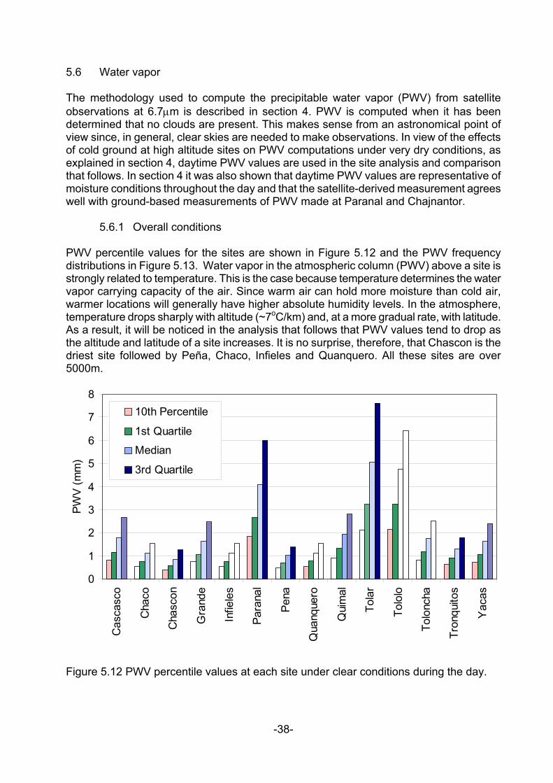
5.6 Water vapor The methodology used to compute the precipitable water vapor (PWV) from satellite observations at 6.7µm is described in section 4. PWV is computed when it has been determined that no clouds are present. This makes sense from an astronomical point of view since, in general, clear skies are needed to make observations. In view of the effects of cold ground at high altitude sites on PWV computations under very dry conditions, as explained in section 4, daytime PWV values are used in the site analysis and comparison that follows. In section 4 it was also shown that daytime PWV values are representative of moisture conditions throughout the day and that the satellite-derived measurement agrees well with ground-based measurements of PWV made at Paranal and Chajnantor. 5.6.1 Overall conditions

PWV percentile values for the sites are shown in Figure 5.12 and the PWV frequency distributions in Figure 5.13. Water vapor in the atmospheric column (PWV) above a site is strongly related to temperature. This is the case because temperature determines the water vapor carrying capacity of the air. Since warm air can hold more moisture than cold air, warmer locations will generally have higher absolute humidity levels. In the atmosphere, temperature drops sharply with altitude (~7oC/km) and, at a more gradual rate, with latitude. As a result, it will be noticed in the analysis that follows that PWV values tend to drop as the altitude and latitude of a site increases. It is no surprise, therefore, that Chascon is the driest site followed by Peña, Chaco, Infieles and Quanquero. All these sites are over 5000m.

0

1

2

3

4

5

6

7

8

Cas

casc

o

Cha

co

Cha

scon

Gra

nde

Infie

les

Para

nal

Pena

Qua

nque

ro

Qui

mal

Tola

r

Tolo

lo

Tolo

ncha

Tron

quito

s

Yac

as

PWV

(mm

)

10th Percentile

1st Quartile

Median

3rd Quartile

Figure 5.12 PWV percentile values at each site under clear conditions during the day.

-38-

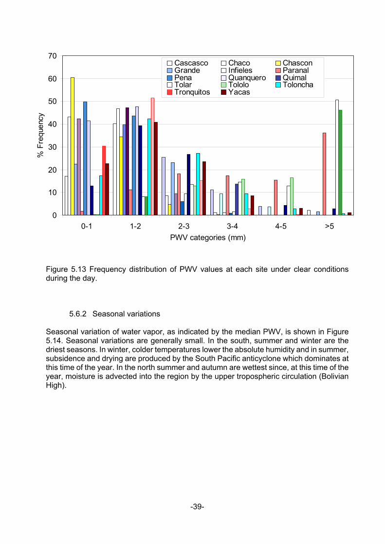
0

10

20

30

40

50

60

70

0-1 1-2 2-3 3-4 4-5 >5PWV categories (mm)

% F

requ

ency

Cascasco Chaco ChasconGrande Infieles ParanalPena Quanquero QuimalTolar Tololo TolonchaTronquitos Yacas

Figure 5.13 Frequency distribution of PWV values at each site under clear conditions during the day. 5.6.2 Seasonal variations Seasonal variation of water vapor, as indicated by the median PWV, is shown in Figure 5.14. Seasonal variations are generally small. In the south, summer and winter are the driest seasons. In winter, colder temperatures lower the absolute humidity and in summer, subsidence and drying are produced by the South Pacific anticyclone which dominates at this time of the year. In the north summer and autumn are wettest since, at this time of the year, moisture is advected into the region by the upper tropospheric circulation (Bolivian High).

-39-

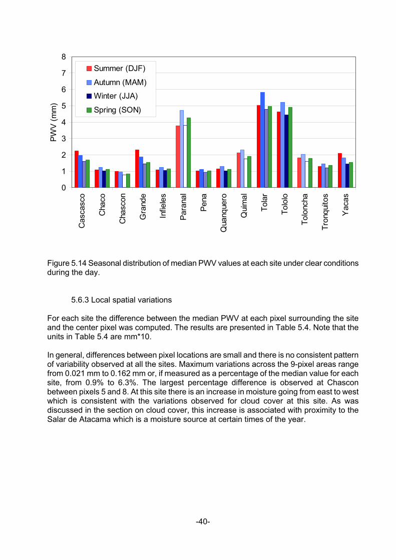
0

1

2

3

4

5

6

7

8

Cas

casc

o

Cha

co

Cha

scon

Gra

nde

Infie

les

Para

nal

Pena

Qua

nque

ro

Qui

mal

Tola

r

Tolo

lo

Tolo

ncha

Tron

quito

s

Yac

as

PWV

(mm

)

Summer (DJF)

Autumn (MAM)

Winter (JJA)

Spring (SON)

Figure 5.14 Seasonal distribution of median PWV values at each site under clear conditions during the day. 5.6.3 Local spatial variations

For each site the difference between the median PWV at each pixel surrounding the site and the center pixel was computed. The results are presented in Table 5.4. Note that the units in Table 5.4 are mm*10. In general, differences between pixel locations are small and there is no consistent pattern of variability observed at all the sites. Maximum variations across the 9-pixel areas range from 0.021 mm to 0.162 mm or, if measured as a percentage of the median value for each site, from 0.9% to 6.3%. The largest percentage difference is observed at Chascon between pixels 5 and 8. At this site there is an increase in moisture going from east to west which is consistent with the variations observed for cloud cover at this site. As was discussed in the section on cloud cover, this increase is associated with proximity to the Salar de Atacama which is a moisture source at certain times of the year.

-40-

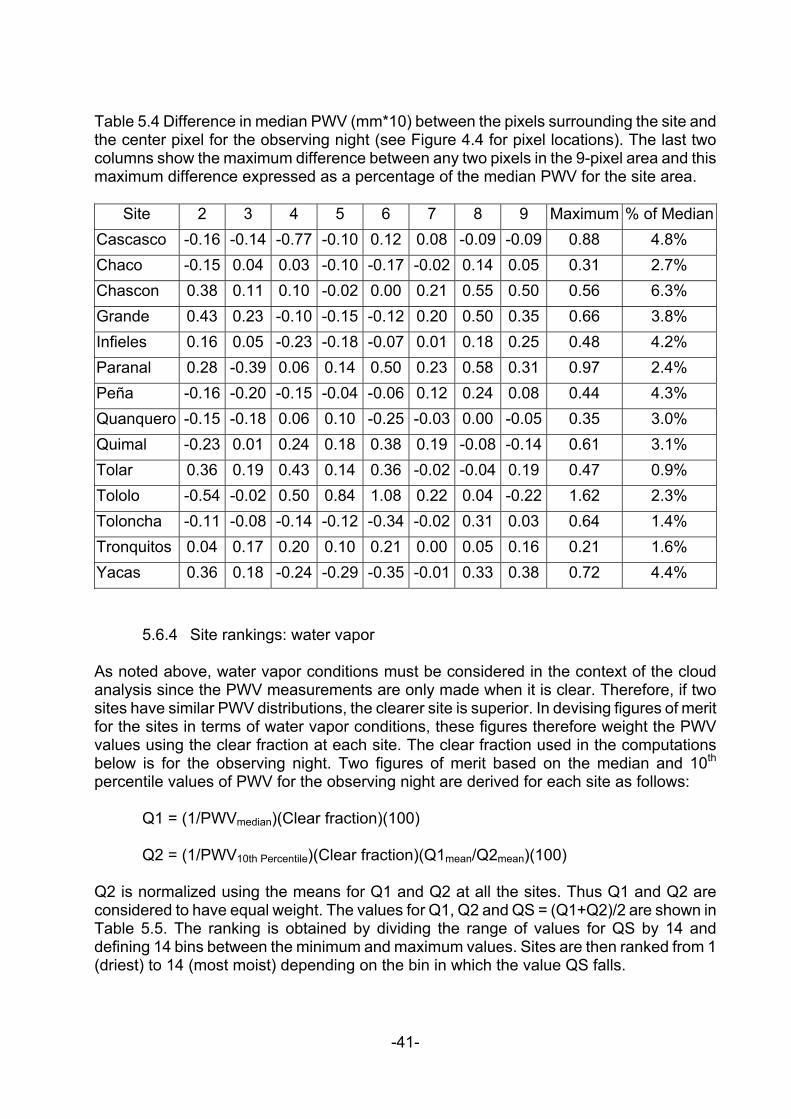
Table 5.4 Difference in median PWV (mm*10) between the pixels surrounding the site and the center pixel for the observing night (see Figure 4.4 for pixel locations). The last two columns show the maximum difference between any two pixels in the 9-pixel area and this maximum difference expressed as a percentage of the median PWV for the site area.

Site 2 3 4 5 6 7 8 9 Maximum % of MedianCascasco -0.16 -0.14 -0.77 -0.10 0.12 0.08 -0.09 -0.09 0.88 4.8% Chaco -0.15 0.04 0.03 -0.10 -0.17 -0.02 0.14 0.05 0.31 2.7% Chascon 0.38 0.11 0.10 -0.02 0.00 0.21 0.55 0.50 0.56 6.3% Grande 0.43 0.23 -0.10 -0.15 -0.12 0.20 0.50 0.35 0.66 3.8% Infieles 0.16 0.05 -0.23 -0.18 -0.07 0.01 0.18 0.25 0.48 4.2% Paranal 0.28 -0.39 0.06 0.14 0.50 0.23 0.58 0.31 0.97 2.4% Peña -0.16 -0.20 -0.15 -0.04 -0.06 0.12 0.24 0.08 0.44 4.3% Quanquero -0.15 -0.18 0.06 0.10 -0.25 -0.03 0.00 -0.05 0.35 3.0% Quimal -0.23 0.01 0.24 0.18 0.38 0.19 -0.08 -0.14 0.61 3.1% Tolar 0.36 0.19 0.43 0.14 0.36 -0.02 -0.04 0.19 0.47 0.9% Tololo -0.54 -0.02 0.50 0.84 1.08 0.22 0.04 -0.22 1.62 2.3% Toloncha -0.11 -0.08 -0.14 -0.12 -0.34 -0.02 0.31 0.03 0.64 1.4% Tronquitos 0.04 0.17 0.20 0.10 0.21 0.00 0.05 0.16 0.21 1.6% Yacas 0.36 0.18 -0.24 -0.29 -0.35 -0.01 0.33 0.38 0.72 4.4%

5.6.4 Site rankings: water vapor As noted above, water vapor conditions must be considered in the context of the cloud analysis since the PWV measurements are only made when it is clear. Therefore, if two sites have similar PWV distributions, the clearer site is superior. In devising figures of merit for the sites in terms of water vapor conditions, these figures therefore weight the PWV values using the clear fraction at each site. The clear fraction used in the computations below is for the observing night. Two figures of merit based on the median and 10th percentile values of PWV for the observing night are derived for each site as follows: Q1 = (1/PWVmedian)(Clear fraction)(100) Q2 = (1/PWV10th Percentile)(Clear fraction)(Q1mean/Q2mean)(100) Q2 is normalized using the means for Q1 and Q2 at all the sites. Thus Q1 and Q2 are considered to have equal weight. The values for Q1, Q2 and QS = (Q1+Q2)/2 are shown in Table 5.5. The ranking is obtained by dividing the range of values for QS by 14 and defining 14 bins between the minimum and maximum values. Sites are then ranked from 1 (driest) to 14 (most moist) depending on the bin in which the value QS falls.

-41-

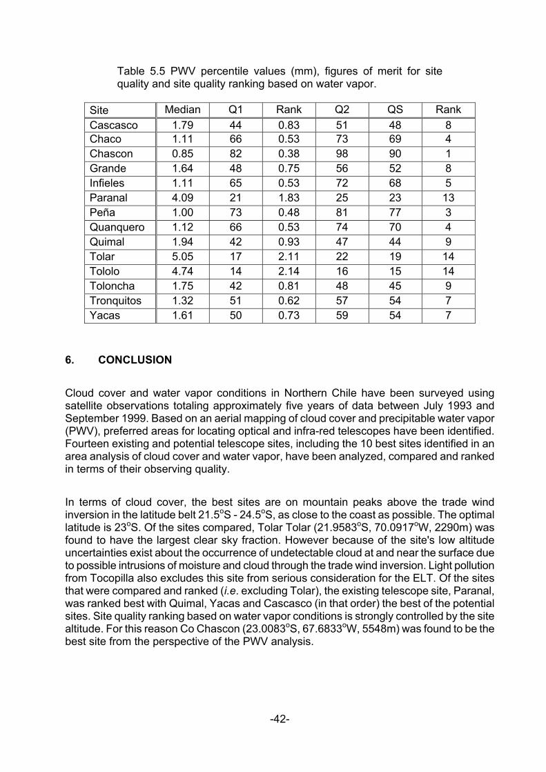
Table 5.5 PWV percentile values (mm), figures of merit for site quality and site quality ranking based on water vapor.

Site Median Q1 Rank Q2 QS Rank Cascasco 1.79 44 0.83 51 48 8 Chaco 1.11 66 0.53 73 69 4 Chascon 0.85 82 0.38 98 90 1 Grande 1.64 48 0.75 56 52 8 Infieles 1.11 65 0.53 72 68 5 Paranal 4.09 21 1.83 25 23 13 Peña 1.00 73 0.48 81 77 3 Quanquero 1.12 66 0.53 74 70 4 Quimal 1.94 42 0.93 47 44 9 Tolar 5.05 17 2.11 22 19 14 Tololo 4.74 14 2.14 16 15 14 Toloncha 1.75 42 0.81 48 45 9 Tronquitos 1.32 51 0.62 57 54 7 Yacas 1.61 50 0.73 59 54 7

6. CONCLUSION Cloud cover and water vapor conditions in Northern Chile have been surveyed using satellite observations totaling approximately five years of data between July 1993 and September 1999. Based on an aerial mapping of cloud cover and precipitable water vapor (PWV), preferred areas for locating optical and infra-red telescopes have been identified. Fourteen existing and potential telescope sites, including the 10 best sites identified in an area analysis of cloud cover and water vapor, have been analyzed, compared and ranked in terms of their observing quality. In terms of cloud cover, the best sites are on mountain peaks above the trade wind inversion in the latitude belt 21.5oS - 24.5oS, as close to the coast as possible. The optimal latitude is 23oS. Of the sites compared, Tolar Tolar (21.9583oS, 70.0917oW, 2290m) was found to have the largest clear sky fraction. However because of the site's low altitude uncertainties exist about the occurrence of undetectable cloud at and near the surface due to possible intrusions of moisture and cloud through the trade wind inversion. Light pollution from Tocopilla also excludes this site from serious consideration for the ELT. Of the sites that were compared and ranked (i.e. excluding Tolar), the existing telescope site, Paranal, was ranked best with Quimal, Yacas and Cascasco (in that order) the best of the potential sites. Site quality ranking based on water vapor conditions is strongly controlled by the site altitude. For this reason Co Chascon (23.0083oS, 67.6833oW, 5548m) was found to be the best site from the perspective of the PWV analysis.

-42-

7. REFERENCES Brest, C.L., W.B. Rossow, and M. Roiter, 1997: Update of Radiance Calibrations for ISCCP J. Atmos. Ocean Tech., 14, 1091-1109. Campbell, G.G, K.R. Dean and T.H. Vonder Haar, 1997: GOES data from GOES NEXT series of satellites. ISCCP Sector Processing Center. Cooperative Institute for Research in the Atmosphere, Colorado State University, Fort Collins, Colorado. (www.cira.colostate. edu/climate/isccp/isccpspc.htm). Erasmus, D. Andre, and R. Peterson, 1996: Feasibility Study and Development of Software Computer Code for Cloud Cover and Water Vapor Forecasts: Phase I. European Southern Observatories Report VLT-TRE-ERA-17440-1038. Erasmus, D. Andre, and P. R. Stanko, 1997: Feasibility Study and Development of Software Computer Code for Cloud Cover and Water Vapor Forecasts: Phase II - Parameter Definitions and Requirements for an Operational System. European Southern Observatories, Report No. VLT-TRE-ERA-17440-1039. Erasmus, D.A., and D.S. Maartens, 1999: Operational Forecasts of Cirrus Cloud Cover and Water Vapor Above Paranal and La Silla Observatories. Final report, European Southern Observatories contract No. 2538/VPS/97/9480/HWE Erasmus, D.A., and D.S. Maartens, 2001: Maintenance, Upgrade and Verification of Operational Forecasts of Cloud Cover and Water Vapor Above Paranal and La Silla Observatories. Draft version of final report, European Southern Observatories contract No. 58311/ODG/99/8362/GWI/LET. Erasmus, D.A. and M. Sarazin, 2000: Forecasting Precipitable Water Vapor and Cirrus Cloud Cover For Astronomical Observatories: Satellite image processing guided by synoptic model dissemination data. SPIE Conference on Image and Signal Processing for Remote Sensing IV. Paper SPIE-4168, Barcelona. 25-29 September, 2000. Erasmus, D.A. and M. Sarazin, 2000: Utilizing Satellite Data For Evaluation and Forecasting Applications At Astronomical Sites. IAU SITE2000 Conference: Astronomical Site Evaluation in the Visible and Radio Range. Marrakesh, Morocco, 13-17 November, 2000. Proceedings. In Press. Rao, P.K., S.J. Holmes, R.K. Anderson, J.S. Winston and P.E. Lehr, Eds., 1990: Weather Satellites: Systems, Data and Environmental Applications. American Meteorological Society, Boston, 503pp.

-43-

Rossow, W.B., C.L. Brest, and M. Roiter, 1995: International Satellite Cloud Climatology Project (ISCCP) Update of Radiance Calibrations. WMO/TD.-No. 736. World Meteorological Organization. Sarazin, M. 1997: A Cloudy Night Again? Blame El Niño! - A study of the impact of El Niño on the cloud cover above ESO observatories in Chile. ESO Messenger, No. 90 � December 1997. Soden, B.J., and F.P. Bretherton, 1993: Upper tropospheric relative humidity from the GOES 6.7µm channel: Method and climatology for July 1987. J. Geophys. Res. 96, 16669-16688. Soden, B.J., and F.P. Bretherton, 1996: Interpretation of TOVS water vapor radiances in terms of layer-average relative humidities: Method and climatology for the upper, middle and lower troposphere. J. Geophys. Res. 101, 9333-9343. Walker, A. and R. Blum, 2001:Site Testing In Chile In The Context Of a 30-100m Telescope. www.ctio.noao.edu/sitetests/.

-44-

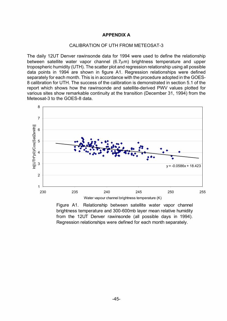
APPENDIX A

CALIBRATION OF UTH FROM METEOSAT-3

The daily 12UT Denver rawinsonde data for 1994 were used to define the relationship between satellite water vapor channel (6.7µm) brightness temperature and upper tropospheric humidity (UTH). The scatter plot and regression relationship using all possible data points in 1994 are shown in figure A1. Regression relationships were defined separately for each month. This is in accordance with the procedure adopted in the GOES-8 calibration for UTH. The success of the calibration is demonstrated in section 5.1 of the report which shows how the rawinsonde and satellite-derived PWV values plotted for various sites show remarkable continuity at the transition (December 31, 1994) from the Meteosat-3 to the GOES-8 data.

Figure A1. Relationship between satellite water vapor channelbrightness temperature and 300-600mb layer mean relative humidity from the 12UT Denver rawinsonde (all possible days in 1994).Regression relationships were defined for each month separately.

y = -0.0586x + 18.423

1

2

3

4

5

6

7

8

230 235 240 245 250 255Water vapour channel brightness temperature (K)

ln[(U

TH*p

0)/C

os(S

atZe

nith

)]

-45-

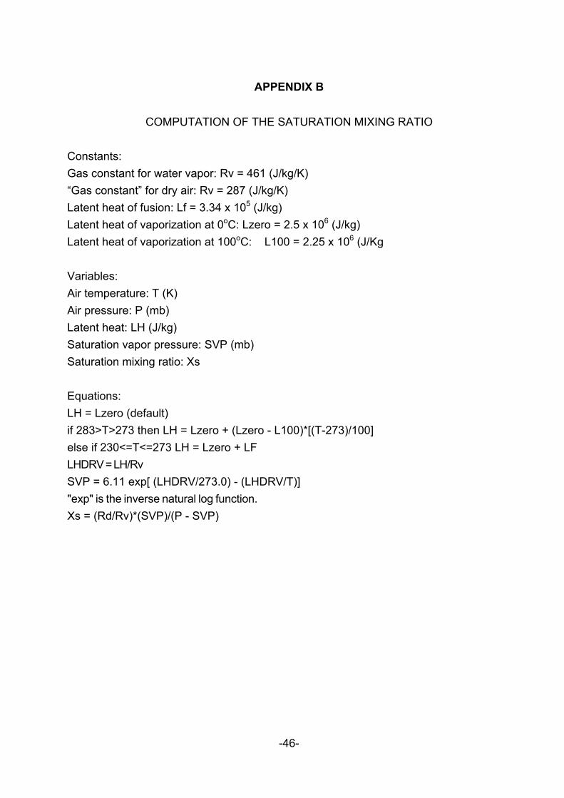
-46-

APPENDIX B

COMPUTATION OF THE SATURATION MIXING RATIO

Constants: Gas constant for water vapor: Rv = 461 (J/kg/K) “Gas constant” for dry air: Rv = 287 (J/kg/K) Latent heat of fusion: Lf = 3.34 x 105 (J/kg) Latent heat of vaporization at 0oC: Lzero = 2.5 x 106 (J/kg) Latent heat of vaporization at 100oC: L100 = 2.25 x 106 (J/Kg Variables: Air temperature: T (K) Air pressure: P (mb) Latent heat: LH (J/kg) Saturation vapor pressure: SVP (mb) Saturation mixing ratio: Xs Equations: LH = Lzero (default) if 283>T>273 then LH = Lzero + (Lzero - L100)*[(T-273)/100] else if 230<=T<=273 LH = Lzero + LF LHDRV = LH/Rv SVP = 6.11 exp[ (LHDRV/273.0) - (LHDRV/T)] "exp" is the inverse natural log function. Xs = (Rd/Rv)*(SVP)/(P - SVP)