a science based emission factor for particulate …
TRANSCRIPT

A SCIENCE BASED EMISSION FACTOR FOR PARTICULATE MATTER
EMITTED FROM COTTON HARVESTING
A Dissertation
by
JOHN DAVID WANJURA
Submitted to the Office of Graduate Studies of Texas A&M University
in partial fulfillment of the requirements for the degree of
DOCTOR OF PHILOSOPHY
May 2008
Major Subject: Biological and Agricultural Engineering
A SCIENCE BASED EMISSION FACTOR FOR PARTICULATE MATTER
EMITTED FROM COTTON HARVESTING
A Dissertation
by
JOHN DAVID WANJURA
Submitted to the Office of Graduate Studies of Texas A&M University
in partial fulfillment of the requirements for the degree of
DOCTOR OF PHILOSOPHY
Approved by:
Chair of Committee, Calvin B. Parnell, Jr. Committee Members, Bryan W. Shaw Sergio C. Capareda Dennis L. O’Neal Head of Department, Gerald L. Riskowski
May 2008
Major Subject: Biological and Agricultural Engineering
iii
ABSTRACT
A Science Based Emission Factor for Particulate Matter Emitted from Cotton
Harvesting. (May 2008)
John David Wanjura, B.S., Texas A&M University;
M.S. Texas A&M University
Chair of Advisory Committee: Dr. Calvin B. Parnell, Jr.
Poor regional air quality in some states across the US cotton belt has resulted in
increased pressure on agricultural sources of particulate matter (PM) from air pollution
regulators. Moreover, inaccurate emission factors used in the calculation of annual
emissions inventories led to the identification of cotton harvesting as a significant source
of PM10 in California and Arizona. As a result, cotton growers in these states are now
required to obtain air quality permits and submit management practice plans detailing
the actions taken by the producer to reduce fugitive PM emissions from field operations.
The objective of this work was to develop accurate PM emission factors for cotton
harvesting in terms of total suspended particulate (TSP), PM10, and PM2.5.
Two protocols were developed and used to develop PM emission factors from
cotton harvesting operations on three farms in Texas during 2006 and 2007. Protocol
one utilized TSP concentrations measured downwind of harvesting operations with
meteorological data measured onsite in a dispersion model to back-calculate TSP
emission flux values. Flux values, determined with the regulatory dispersion models
ISCST3 and AERMOD, were converted to emission factors and corrected with results
from particle size distribution (PSD) analyses to report emission factors in terms of PM10
and PM2.5. Emission factors were developed for two-row (John Deere 9910) and six-
row (John Deere 9996) cotton pickers with protocol one. The uncertainty associated
with the emission factors developed through protocol one resulted in no significant
difference between the emission factors for the two machines.

iv
Under the second protocol, emission concentrations were measured onboard the
six-row cotton picker as the machine harvested cotton. PM10 and PM2.5 emission factors
were developed from TSP emission concentration measurements converted to emission
rates using the results of PSD analysis. The total TSP, PM10, and PM2.5 emission factors
resulting from the source measurement protocol are 1.64 ± 0.37, 0.55 ± 0.12, and 1.58E-
03 ± 4.5E-04 kg/ha, respectively. These emission factors contain the lowest uncertainty
and highest level of precision of any cotton harvesting PM emission factors ever
developed. Thus, the emission factors developed through the source sampling protocol
are recommended for regulatory use.

v
ACKNOWLEDGEMENTS
This research effort has been very challenging, trying, and rewarding. The
success of this work is in no way due to the sole efforts of one person, but through the
extraordinary efforts of a wonderful group of people, this project has experienced great
success. It is my intention to thank each and every person involved in this work from
the bottom of my heart.
First I would like to thank God for his continuing graces and blessings in my life.
I owe everything to Him for providing me the opportunity of life. I pray that my life
may be lived by His will and as a gift back to Him.
To my wife, Karen, your love and encouragement through this journey has made
the experience a joy for me. I love you and I thank God for you each and every day. I
look forward to what the future holds for us.
To my family, thank you for your love, support, and encouragement. I would
like to thank my mother and father for their love and guidance through out my life.
Mom, your love and care continues to support me through everyday. Dad, you are a
great role model and thank you for your wisdom and ability to help me put things in
perspective.
To Vic, Amy, Eric, and Christine, thank you for your encouragement during my
time at A&M. I look forward to working and living in Lubbock and to all of the time we
will be able to spend together. There really is nothing like going home!
The extraordinary efforts of “Parnell’s Crew” have made the execution of this
project not only possible, but a joy. Without you all we couldn’t have done this! One
problem with spending ten years of your life in a place like Texas A&M is that you have
a hard time remembering everyone who has helped you along your way. Nonetheless,
I’ll give it a try. Brock, Bonz, Barry, Clay, Craig, Brad, Mike, Amber, Ling, Amy, Lee,
Sergio, Ryan, “Tree”, Jackie, Shay, Jing, Mark, Nathaniel, Cale, Shane, Clint, Atilla,
“Stanley”, Toni, Scott, Lee, Stewart, Jen, Kaela, Mary, Froi, Joan, Yufeng, Sam,
“Monkey Man” Shane Morgan, Josh, Kyle, Russ, Matt, Britt, Mark, Dustin, you guys

vi
are great friends and I wish the best for all of you in the future. I can’t thank you enough
for your help.
To Dr. Parnell, thank you for your support and help throughout my experience at
A&M. I am leaving A&M with that grin we spoke about. Your example of what an
engineer, scientist, role model, mentor and friend has made an everlasting impression on
me. Thank you for all of this!
I would like to thank my committee members, Drs. Parnell, Shaw, Capareda, and
O’Neal, for their help and encouragement through this process. Thank you for giving
me the chance to further develop my skills as an engineer through this Ph. D. program.
Also, a big word of thanks is due to Dr. Lacey for having an open ear and the
willingness to help me in this effort. Thank you also to the staff of the BAEN
department for your help in this process.
I would also like to thank Mr. Tim Deutsch, Dr. Ed Barnes, and Dr. Bill Norman,
from John Deere, Cotton Incorporated, and The Cotton Foundation, respectively, for
providing the financial assistance needed to conduct this research. Further thanks are
due to John Deere for providing the 9996 cotton picker used in the project. Thank you
for your help and I look forward to working with you again in the future.
A special word of thanks goes to all of the people working on my behalf within
USDA-ARS to give me the opportunity to pursue further education in agricultural
engineering. I would especially like to thank Dr. Alan Brashears, Dr. Jeff Carroll, Dr.
Michael Buser, Dr. Dan Upchurch, Wanda Robertson, and all of the folks at the Cotton
Production and Processing Research Unit for helping to make this a success. Further
thanks go to the Cotton Production and Processing Research Unit for allowing us the use
of the 9910 model cotton picker over these past two years.
vii
TABLE OF CONTENTS
Page
ABSTRACT .............................................................................................................. iii
ACKNOWLEDGEMENTS ...................................................................................... v
TABLE OF CONTENTS .......................................................................................... vii
LIST OF FIGURES................................................................................................... ix
LIST OF TABLES .................................................................................................... xii
CHAPTER
I INTRODUCTION................................................................................ 1
Objective ........................................................................................ 6
II FIELD SITE CHARACTERIZATION................................................ 8
Introduction .................................................................................... 8 Sampling Site Descriptions ............................................................ 8 Sampling Site Characterization Methods ....................................... 18 Results ............................................................................................ 21
III EMISSION FACTOR DEVELOPMENT PROTOCOL I: UPWIND/DOWNWIND SAMPLING WITH DISPERSION MODELING ................................................................ 26
Introduction .................................................................................... 26 Particulate Matter Concentration Measurements ........................... 29 Dispersion Modeling ...................................................................... 34 Results ............................................................................................ 52
IV EMISSION FACTOR DEVELOPMENT PROTOCOL II: SOURCE MEASUREMENT OF EMISSION CONCENTRATIONS.......................................................................... 71
Introduction .................................................................................... 71 Prototype Development and First Year Testing............................. 72 Seed Cotton Separation System Design Modification and Evaluation.......................................................... 78 System Development and Evaluation Results................................ 94 Source Measurement of Cotton Picker PM Emissions .................. 107

viii
CHAPTER ........................................................................................................ Page
V PARTICLE SIZE DISTRIBUTION AND PARTICLE DENSITY ANALYSIS OF PARTICULATE MATTER SAMPLES ................... 119
Introduction .................................................................................... 119 Methods.......................................................................................... 120 Results ............................................................................................ 122
VI SUMMARY AND CONCLUSIONS................................................... 142
Future Work ................................................................................... 145
REFERENCES.......................................................................................................... 146
APPENDIX A SOIL SIEVING PROCEDURE ..................................................... 152
APPENDIX B METEOROLOGICAL DATA DEVELOPED FOR USE IN AERMOD FROM 3D SONIC ANEMOMETER MEASUREMENTS ....................................................................... 156
APPENDIX C TSP AND PM10 CONCENTRATION MEASUREMENTS TAKEN DURING THE SAMPLING EVENTS DURING 2006 AND 2007 ............................................................................. 163
APPENDIX D SYSTEMATIC UNCERTAINTY ANALYSIS FOR THE SOURCE SAMPLING SYSTEM.................................................. 186
APPENDIX E ASH ANALYSIS RESULTS FOR PARTICULATE MATTER LESS THAN 100 MICROMETERS CAPTURED IN THE SOURCE SAMPLER CYCLONE BUCKET................................ 192
APPENDIX F TEST SUMMARY SHEETS FOR THE SOURCE SAMPLING TESTS CONDUCTED DURING 2007......................................... 195
APPENDIX G PARTICLE SIZE DISTRIBUTION RESULT STATISTICS FOR THE TSP SAMPLER FILTERS AND PM CAPTURED BY THE SOURCE SAMPLER ..................................................... 206
VITA ......................................................................................................................... 212
ix
LIST OF FIGURES
Page
Figure 1 United States cotton yield between 1977 and 2007 .......................... 4
Figure 2 Layout of the test plots used in the testing at farm 1......................... 9
Figure 3 Layout of the test plots used in the tests conducted on farm 2.......... 11
Figure 4 Layout of test plots on farm 3 ........................................................... 13
Figure 5 Aerial image of farm 3 showing the test plot layout used in 2007.... 16
Figure 6 Image of air washing system shown with seed cotton sample .......... 19
Figure 7 Typical arrangement of collocated TSP/PM10 samplers around the test plots....................................................................................... 30
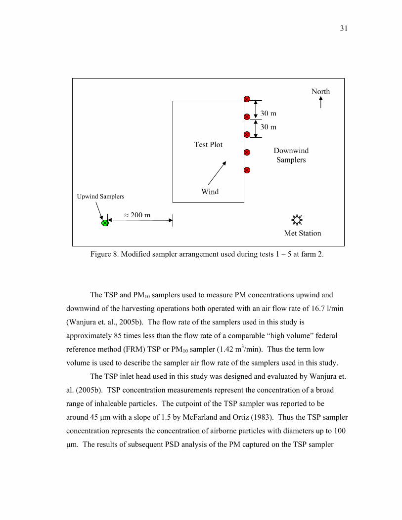
Figure 8 Modified sampler arrangement used during tests 1 – 5 at farm 2. .... 31
Figure 9 Schematic diagram of the separation system designed to separate the seed cotton from the air stream from duct 3 of the six-row harvester. ........................................................................................... 73
Figure 10 Detail drawing of separator box design 1 showing interior curved baffle (side view)............................................................................... 74
Figure 11 Schematic drawing of separator box design 1 with general dimensions shown (isometric view).................................................. 75
Figure 12 Photo of seed cotton separation system mounted in the testing frame configured with the seed cotton feeder and fan system .......... 79
Figure 13 Schematic drawing of separator box design 2 illustrating the straight back wall design with the brush wheel moved to the rear of the separator box. .......................................................................... 81
Figure 14 Detail drawing of separator box design 2 shown with interior baffle design 5 (side view) ................................................................ 82
Figure 15 Schematic drawing of separator box design 2 showing general dimensions (isometric view) ............................................................. 83
Figure 16 Schematic showing curved baffle dimensions for baffles 1, 2, 3, and 4 ...................................................................................... 85
Figure 17 Schematic showing straight baffle dimensions for baffles 5, 6, and 7 .......................................................................................... 85

x
Page
Figure 18 Schematic diagram of air velocity probe locations across the exit duct (numbers inside the equal area squares represent probe locations) ........................................................................................... 87
Figure 19 Schematic diagram of concentration sampling locations in the exit duct (numbers represent sampling locations).................................... 89
Figure 20 Linear motion dust feeding system used to feed corn starch into the testing system at 12 g/min. .......................................................... 90
Figure 21 Photograph of the source sampling system mounted on the test frame.................................................................................................. 94
Figure 22 Seed cotton penetration test results for separation box design 1 tested with baffles 1, 2, and 3 at seed cotton feeding rates of 22.7, 45.4, and 68.1 kg/min........................................................................ 95
Figure 23 Seed cotton penetration test results for separation box design 2 tested with baffles 1 - 7 at seed cotton feeding rates of 22.7, 45.4, and 68.1 kg/min................................................................................. 97
Figure 24 Normalized velocity measurements at nine coplanar points across the cross section of the exit duct ....................................................... 99
Figure 25 Comparison of the duct mean concentration to the center point ...... concentration by test.......................................................................... 102
Figure 26 Center point, mass weighted average, and input corn starch PSDs . measured during test 4....................................................................... 106
Figure 27 Photograph of the six row harvester traveling down rows of cotton (average plant height 41 – 51 cm) with the row units and fan not engaged in order to measure the concentration of PM generated by the interaction of the harvester wheels and the soil surface (samplers located to the left of the harvester) ................................... 116
Figure 28 Percent volume vs. ESD particle diameter PSDs for the air wash PM <100 μm (Air Wash Material), PM on the TSP sampler filter .. (Ambient TSP Sampler Filter), soil material < 75 μm (Soil Material), source sampler cyclone bucket material <100 μm (SS Cyclone Bucket Material), and PM on the source sampler filters (Source Sampler Filter) from test 7 on farm 1 during 2006.............. 125

xi
Page
Figure 29 Percent volume vs. ESD particle diameter PSDs for the air wash PM <100 μm (Air Wash Material), PM on the TSP sampler filter .. (Ambient TSP Sampler Filter), soil material < 75 μm (Soil Material), source sampler cyclone bucket material <100 μm (SS Cyclone Bucket Material), and PM on the source sampler filters (Source Sampler Filter) from test 7 on farm 2 during 2006.............. 126
Figure 30 Percent volume vs. ESD particle diameter PSDs for the air wash PM <100 μm (Air Wash Material), PM on the TSP sampler filter ... (Ambient TSP Sampler Filter), and soil material < 75 μm (Soil Material) from test 1 on farm 3 during 2006............................ 127
Figure 31 Average PSD results for the soil material <75 μm from farm 1, 2, and 3 .................................................................................................. 128
Figure 32 Average PSD results of the air wash material from farm 1, 2, and 3 .......................................................................................... 129
Figure 33 Composite source sampler PSDs for the four source sampling tests conducted at farm 1 and farm 2......................................................... 131
Figure 34 PSD of a downwind TSP sampler from test 20 at farm 3 during 2007 shown with the farm average lognormal PSD of the TSP sampler filters (MMD = 14.7, GSD = 2.23)...................................... 135
Figure 35 Average PSD for the soil material < 75μm collected from farm 3 during 2007 .................................................................................... 136
Figure 36 Average PSD of the core samples cut from the source sampler filters obtained during the tests conducted at farm 3 during 2007. ... 137
Figure 37 Average PSD of the PM < 100 μm air washed from the source sampler cyclone bucket from the tests conducted on farm 3 during 2007. ...................................................................................... 139
Figure 38 Average PSDs for the source sampler filters, PM < 100 μm captured in the source sampler cyclone bucket, and the mass weighted average composite PSD for the tests conducted on farm 3 during 2007............................................................................ 140
xii
LIST OF TABLES
Page
Table 1 Experimental design of the sampling tests conducted at farm 1 ....... 10
Table 2 Design of the experiments conducted at farm 2 ................................ 12
Table 3 Order of the experiments conducted at farm 3 in 2006..................... 14
Table 4 Order of experiments conducted on farm 3 during 2007. ................. 17
Table 5 Moisture content analysis results of the hand harvested seed cotton samples taken during the tests at farms 1, 2, and 3 during 2006
and 2007. ........................................................................................... 22
Table 6 Sieve analysis results for soil samples collected from farms 1, 2, and 3 during 2006 and 2007. The values presented in the table represent the percent of the total material processed remaining within the size range.......................................................................... 24
Table 7 Surface soil moisture content measurements from farm 3 during 2007............................................................................ 25
Table 8 Key to Solar Radiation Delta – T method for estimating day time Pasquill-Gifford stability categories (EPA, 2000) ............................ 37
Table 9 Key to Solar Radiation Delta – T method for estimating night time Pasquill-Gifford stability categories (EPA, 2000) ............................ 37
Table 10 Concentration measurement results and average sampler PM10/TSP concentration ratios from the sampling conducted at farm 1 during 2006............................................................................ 52
Table 11 Concentration measurement results and average sampler PM10/TSP concentration ratios from the sampling conducted at farm 2 during 2006............................................................................ 53
Table 12 Concentration measurement results and average sampler PM10/TSP concentration ratios from the sampling conducted at farm 3 during 2006............................................................................ 53
Table 13 Concentration measurement results and average sampler PM10/TSP concentration ratios from the sampling conducted at farm 3 during 2007............................................................................ 54
xiii
Page
Table 14 Emission factor results from the dispersion modeling procedure using ISCST3 for farm 1 during 2006............................................... 56
Table 15 Emission factor results from the dispersion modeling procedure using ISCST3 for farm 2 during 2006............................................... 57
Table 16 Emission factor results from the dispersion modeling procedure using ISCST3 for farm 3 during 2006............................................... 58
Table 17 Emission factor results from the dispersion modeling procedure using ISCST3 for farm 3 during 2007............................................... 59
Table 18 Summary of ISCST3 emission factor results combining the data from farms 1, 2, and 3 (2006) and farm 3 (2007).............................. 60
Table 19 Emission factor results from the dispersion modeling procedure using AERMOD for farm 3 during 2007 .......................................... 62
Table 20 Correlation analysis results using the emission factor results produced with ISCST3 ...................................................................... 64
Table 21 Correlation analysis results using the emission factor results produced with AERMOD.................................................................. 65
Table 22 Description of the baffles tested in separator box designs 1 and 2 .................................................................................. 84
Table 23 Mass of seed cotton penetrating (g) separator box design 1 with baffles 1, 2, and 3 (see Table 22) at three seed cotton feed rates. ..... 95
Table 24 Mass of seed cotton penetrating (g) separator box design 2 with baffles 1 - 7 (see Table 22) at three seed cotton feed rates. .............. 97
Table 25 Mean normalized air velocity measurements (% of maximum duct velocity) from five replicated tests at three seed cotton feed rates ... 98
Table 26 Concentration data collected at five coplanar locations across the cross section of the exit duct of the seed cotton separation system .............................................................................. 101
Table 27 Summary statistics for the ratio of the air velocity entering the sampling probe to the air velocity passing the probe calculated for five samplers during five concentration tests .................................... 104
xiv
Page
Table 28 AED PSD analysis results of each isokinetic sampling location within the exit duct of the seed cotton separation system ................. 106
Table 29 Source sampling system total deposition test results at 5 and 10 g/min nominal inlet dust feeding rate........................................... 107
Table 30 Six-row harvester emission concentration results for the 10 tests conducted with the source sampling system on farm 3
during 2007 ....................................................................................... 109
Table 31 Six-row harvester emission rates for ten tests conducted with the source sampling system on farm 3 during 2007.......................... 110
Table 32 Six-row harvester emission factors from ten tests performed with the source sampling system on farm 3 during 2007.................. 111
Table 33 Correlation results of the source sampler emission rate data with area, yield, test duration, soil mass % < 75 μm, soil mass % < 106 μm, seed cotton moisture content, and soil surface moisture content ............................................................................................... 112
Table 34 Emission factors developed using measured TSP concentrations and ISCST3 for tests conducted to quantify the PM emissions generated by the interaction between the harvester wheels and the soil surface......................................................................................... 118
Table 35 Average particle density measurements on soil material less than 75 μm taken from farms 1, 2, and 3 during 2006 and 2007 .............. 122
Table 36 Particle density analysis results for particulate matter less than 100 μm air washed from seed cotton samples taken during 2006..... 123
Table 37 Particle density results of PM <100 μm air washed from material captured in the bucket of the source sampler cyclone during 2007 .. 124
Table 38 MMD (ESD) and GSD of the best fit lognormal curves for the data shown in Figures 28, 29, and 30................................................ 127
Table 39 MMD and GSD values for the best fit lognormal distributions for the average air wash PSDs from farm 1, 2, 3 .................................... 129
Table 40 MMD and GSD values for the best fit lognormal distributions for the composite source sampler PSDs. Also shown are the mass
percentages of PM10 and PM2.5 of the best fit lognormal distributions and PSD data measured by the Coulter Counter .......... 132
Table 41 PSD analysis results of the PM on the TSP filters from farms 1, 2, and 3 ................................................................................ 133
xv
Page Table 42 TSP sampler filter PSD analysis result statistics for samples taken on farm 3 during 2007. The particle density used to convert ESD to AED was 1.59 g/cm3 ..................................................................... 134
Table 43 Soil material < 75μm PSD result statistics from samples collected on farm 3 during 2007....................................................................... 136
Table 44 PSD analysis result statistics for the source sampler filters collected during the tests conducted on farm 3 during 2007............. 138
Table 45 PSD results for the PM < 100 μm air washed from the material captured in the source sampler cyclone bucket from the tests conducted on farm 3 during 2007 ..................................................... 138
Table 46 Result statistics for the mass weighted average composite PSDs developed from the PSDs of the source sampler filters and PM < 100 μm captured in the source sampler cyclone bucket during 2007 ....................................................................................... 141

1
CHAPTER I
INTRODUCTION
Air pollution regulation across the US is implemented and enforced by state air
pollution regulatory agencies (SAPRA). This authority is granted to the SAPRA by the
federal EPA upon approval of the state implementation plan (SIP). The SIP outlines the
steps that a state will take to ensure that the air quality within the state meets federal air
quality standards (CFR, 1996). The National Ambient Air Quality Standards (NAAQS)
are established for six criteria pollutants including SOx, NOx, CO, ozone, PM10, and
PM2.5. An area within a state may be classified as a non-attainment area if the ambient
concentration of a criteria pollutant is shown to exceed the NAAQS by measurement or
through dispersion modeling.
On September 21, 2006, EPA finished the five year cyclical review of the PM
NAAQS and published “the most protective suite of national air quality standards for
particle pollution ever” (EPA, 2006). Included in these revisions to the PM NAAQS
were the removal of the annual PM10 standard of 50 μg/m3 and the lowering of the 24
hour average PM2.5 standard from 65 to 35 μg/m3. The EPA based the decision to
implement these NAAQS revisions on an in depth review of the most current and up-to-
date scientific studies which investigated the health related impacts of PM pollution on
certain sensitive populations.
The primary criteria pollutant of interest to the cotton industry is PM10. PM10
refers to the fraction of particulate matter (PM) with aerodynamic equivalent diameter
(AED) less than or equal to 10 micrometers (µm). The 24-hour average NAAQS
concentration limit for PM10 is 150 μg/m3 (Federal Register, 2006). PM2.5 refers to
particles (liquid or solid) that have an AED less than or equal to 2.5 µm. The NAAQS
limits the 24 hour average concentration of PM2.5 to 35 μg/m3. The annual average
____________ This dissertation follows the format and style of Transactions of the ASAE.
2
NAAQS concentration limit for PM2.5 is 15 μg/m3 (Federal Register, 2006).
Historically, the PM2.5 NAAQS has been of little concern to agricultural producers.
Agricultural operations (including cotton production and processing) typically emit PM
with larger particle sizes than urban sources (Wanjura, 2005) and which contain very
few particles smaller than 2.5 µm
Cotton producers in some states across the cotton belt are facing increased
regulatory pressure from SAPRAs due to poor regional air quality (PM10 and PM2.5
NAAQS non-attainment status). Further, cotton producers in California have been
identified as a significant source of PM10 due to the use of a flawed emission factor. As
a result, agricultural producers are required to obtain operating permits from the SAPRA
(CARB, 2003) and submit Conservation Management Practice (CMP) plans detailing the
actions to be taken by the producer to reduce fugitive PM emissions (SJVAPCD, 2004 a
and b). Further, the reduction of the PM2.5 NAAQS accomplished during the five year
review of the NAAQS by EPA in 2006 will present cotton producers with new air
quality regulation challenges due to the lack of accurate emission factors.
Emission factors are estimates of the amount of a pollutant emitted by an
operation per unit of production (i.e. lbs. PM10 per acre of cotton harvested). Emission
factors are used by air pollution regulators to determine annual emissions inventories
and in dispersion models to predict downwind concentrations resulting from the
pollutant emissions from a source.
A limited amount of research has been conducted to quantify the PM10 emissions
from cotton harvesting. A study conducted under contract with the USEPA by Snyder
and Blackwood (1977) reported emissions of particulate matter less than 7 µm (mean
aerodynamic diameter) on the order of 0.96 kg/km2 (8.4*10-3 lbs/acre) for harvesting
operations using cotton pickers. This emission factor represented the total emission
factor from harvesting operations including emissions from the harvesting machine,
trailer loading operations, and trailer transporting operations. It was reported by Snyder
and Blackwood (1977) that particulate matter samplers followed the harvesting machine
at a fixed distance within the plume to collect particulate matter concentrations. The
3
authors stated further that particulate matter concentrations downwind of trailer loading
operations were taken by placing samplers at a fixed downwind distance. It is stated in
AP-42 (EPA, 1995a) that the emission factors reported are based on the following
assumptions:
1. The average speed of the picking machine was 1.34 m/s (3.0 mph),
2. The basket capacity of the picking machine was 109 kg (240 lbs),
3. The capacity of the transport trailers were 6 baskets each, and
4. The average cotton lint yield was 1.17 bales/acre for pickers.
The information given in AP-42 (EPA, 1995a) is based on antiquated harvesting
technology and a flawed protocol. No detail was given as to how the researchers used
measured concentrations to determine the emissions from the harvesting machine. The
same was true for the method used to determine the emission rate from the trailer
loading operation. Did the researchers use a dispersion model to back-calculate the
emission rates from these operations, and if so, which one? Further, the emission factors
reported are based on concentrations of particulate matter less than 7 μm mean
aerodynamic diameter. This size range of particulate matter represents only part of the
regulated size fraction of dust in the US. PM10 concentrations include the mass of all
particles less than 10 μm in aerodynamic diameter.
The harvesting machinery used to develop the emission factors in AP-42 (EPA,
1995a) does not represent the technology that is used today. Today’s machinery can
harvest up to six rows of cotton per pass with basket capacities in the range of 4086 kg
(9000 lbs) (basket volume: 40 m3 or 1400 ft3). Clearly, the machines used to harvest the
US cotton crop today are significantly different from the machines used in the 1970’s,
when the Snyder and Blackwood study was conducted.
Farming practices have also changed resulting in increased yields and field
efficiencies since the 1970’s. In particular, US cotton production has increased from
approximately 10 million bales to around 20 million bales over the last 30 years while
the total production area has remained the same (USDA, 2007). The increase in yield is
due primarily to improved plant varieties producing higher yields and farming practices
4
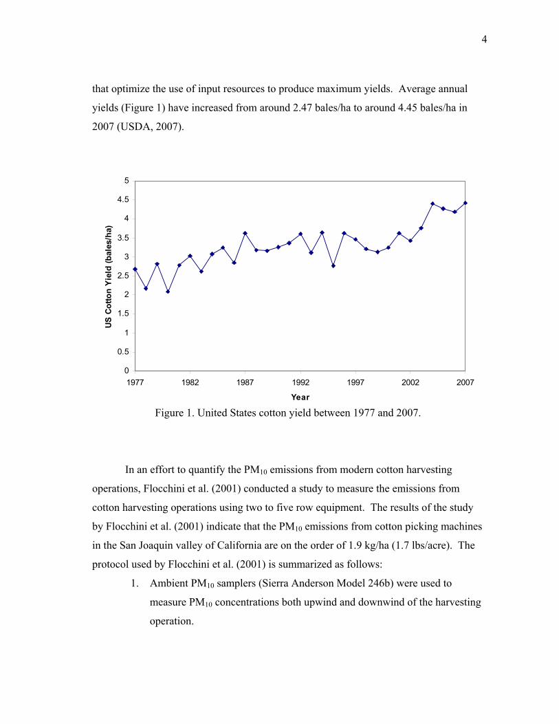
that optimize the use of input resources to produce maximum yields. Average annual
yields (Figure 1) have increased from around 2.47 bales/ha to around 4.45 bales/ha in
2007 (USDA, 2007).
0
0.5
1
1.5
2
2.5
3
3.5
4
4.5
5
1977 1982 1987 1992 1997 2002 2007
Year
US C
otto
n Yi
eld
(bal
es/h
a)
Figure 1. United States cotton yield between 1977 and 2007.
In an effort to quantify the PM10 emissions from modern cotton harvesting
operations, Flocchini et al. (2001) conducted a study to measure the emissions from
cotton harvesting operations using two to five row equipment. The results of the study
by Flocchini et al. (2001) indicate that the PM10 emissions from cotton picking machines
in the San Joaquin valley of California are on the order of 1.9 kg/ha (1.7 lbs/acre). The
protocol used by Flocchini et al. (2001) is summarized as follows:
1. Ambient PM10 samplers (Sierra Anderson Model 246b) were used to
measure PM10 concentrations both upwind and downwind of the harvesting
operation.

5
2. The vertical concentration profile of the dust plume downwind of the
operation was quantified using a series of three mobile towers with PM10
samplers and anemometers mounted at several heights.
3. A LIDAR instrument was also used to help describe the shape of the plume
downwind of the harvesting operation. The results of the LIDAR
instrument give insight as to the shape of the plume as it travels downwind,
but it does not give any reliable indication of the concentration or size of
the particulate matter within the plume.
4. A mass balance box model was used with the concentration data to
determine the area source emission rate from the operation. Several
different methods to describe the shape of the plume were used within the
box model to assess the influence of the plume shape on the estimated
emission factors.
The work by Flocchini et al. (2001) represents the most up-to-date information
regarding PM10 emissions from cotton harvesting operations. However, the sampling
protocol used by Flocchini et al. (2001) contained several components that introduced
significant levels of uncertainty, including:
1. The federal reference method PM10 samplers have been shown to exhibit
substantial over-sampling errors when sampling agricultural dusts. Buser et
al. (2001) indicated that the Federal Reference Method (FRM) PM10
sampler could theoretically overstate PM10 concentrations by as much as
340% when sampling a dust with mass median diameter (MMD) and
geometric standard deviation (GSD) of 20µm and 2.0, respectively. The
over-sampling errors reported by Buser et al. (2001) have been observed in
field work conducted by several sources including Wanjura et al. (2005a)
and Capareda et al. (2005).
2. The box model used to estimate the area source emission rate from the
harvesting operation relies on several assumptions pertaining to the height
of the plume and depth of the emitting area. In addition, the emission rates
6
determined using the box model are specific to the box model and may not
be appropriate to use with another dispersion model. In other words, an
emission rate developed with the box model and subsequently used in the
box model will return the same measured concentrations initially used to
develop the emission rate. However, if the same emission rate is used in
another dispersion model, such as those utilized by SAPRAs, it is likely
that the model will not return the measured concentration values. This is
important from a regulatory standpoint.
For agricultural sources to be equitably regulated, accurate emissions inventories
must be calculated by air pollution regulators using accurate, science-based emission
factors. Along with facilitating the equitable regulation of agricultural sources, accurate
emissions inventories will help regulators and agricultural producers focus their
emissions reduction efforts on the operations or processes that produce the highest level
of emissions.
OBJECTIVE
The main objective of this work was to develop accurate emission factors for PM
emissions originating from modern cotton harvesting operations in terms of PM10, PM2.5,
and TSP. The PM emission factors currently available for use by air pollution regulators
were developed using antiquated harvesting machinery with respect to throughput
capacity and machine size. Two protocols were used to develop PM emission factors
from cotton harvesting operations using machines of two different harvesting capacities.
Emission factors for a two-row John Deere model 9910 and six-row John Deere model
9996 were developed with a protocol employing two dispersion models to back calculate
emission flux values from downwind concentrations and meteorological data measured
onsite. The dispersion models used are Industrial Source Complex Short Term version 3
(ISCST3) and American Meteorological Society/Environmental Protection Agency
Regulatory Model (AERMOD). The second protocol employed a novel source sampling
system designed for use onboard the six-row machine. Source sampling of field

7
operations to develop emission factors has not been performed due to the difficulty
encountered in collecting representative emissions data from agricultural machinery
operating under field conditions. It was anticipated that the emission factors developed
using the source sampling protocol would be the most accurate ever developed. The
emission factors developed under the source sampling protocol allowed for in depth
analysis of the relationship between PM emission rates and crop yield and land area.
Particle size distribution (PSD) analyses were conducted on the PM collected under both
protocols and used to determine PM10 and PM2.5 emission factors from TSP
measurements.
8
CHAPTER II
FIELD SITE CHARACTERIZATION
INTRODUCTION
Field work was conducted at three locations during 2006 and one location during
2007. Three sites were selected for use during the 2006 season to ensure that sufficient
data were collected and that any necessary modifications to the measurement protocols
could be properly evaluated. Such modifications included changes in experimental
design, sampler placement, and test plot size/configuration. A total of twenty three tests
were conducted during 2006 while twenty one were conducted during 2007. The
available area used for testing on farm 3 was increased significantly between 2006 and
2007 allowing for all of the tests conducted in 2007 to be performed at farm 3.
In addition to the PM concentration measurements taken at each location,
additional samples were taken to quantify 1) the moisture content of the seed cotton
during harvest, 2) the soil moisture content during harvest (2007 only), 3) the mass
fraction of soil less than 75 and 104 μm, and 4) the particle density and PSD of the PM
contained in the harvested seed cotton. While the primary focus of the work at each
farm was to collect PM concentration data for emission factor development, these
additional data were taken to help characterize the source of the PM emissions as well as
investigate the relationships between source characteristics and the magnitude of PM
emissions. The protocols used and the results from these analyses are discussed here and
used in further analyses in later sections. All statistical analyses were conducted using
the General Linear Model in SPSS (SPSS 12.0.1, SPSS Inc., Chicago, IL) with α = 0.05
unless specified otherwise.
SAMPLING SITE DESCRIPTIONS
Farm 1 is located approximately 8 km south of El Campo, TX. The dark, clay
soil was fairly wet at the beginning of the four day sampling event but dried out by the
end. The 28.3 ha (70 ac) rectangular field was planted with a 96.5 cm (38 in) row

9
spacing oriented in a north – south pattern. The field was divided into two sections (16.2
ha to the south and 12.1 ha to the north) by a house and grazing area (see Figure 2). The
southern section of the field was subdivided into eight 1.6 ha (4 acre approximate size)
test plots (450 m row length). The northern section was subdivided into four 2.4 ha (6
acre approximate size) test plots (245 m row length). A conventional picker variety of
cotton was grown and the crop was defoliated with one application of Ginstar® (Bayer
Crop Science, Research Triangle Park, NC).
Figure 2. Layout of the test plots used in the testing at farm 1.
12 11 10 9
8 7 6 5 4 3 2 1
N

10
Three treatments were tested in a randomized complete block design (blocked by
day/replication). The three treatments included 1) upwind/downwind sampling of the
PM emissions from the two-row harvester (“2 row”), 2) upwind/downwind sampling of
the PM emissions from the six-row harvester without the source sampling system (“6
row”), and 3) source sampling in conjunction with upwind/downwind sampling of the
six-row harvester emissions (“6 row w/SS”). The experimental design for the tests
conducted at farm 1 is shown in Table 1.
Ten of the original twelve planned sampling tests were conducted at farm 1 due
to unexpected delays caused by equipment failures and the labor intensive nature of the
sampling work. Approximately 6 man hours of labor were required to install and
remove the source sampling system between tests. Moving and resetting the collocated
TSP and PM10 samplers between tests required approximately three to four man hours.
Ten to fourteen hour working days became common place over the duration of the
sampling work conducted at farm 1.
All of the planned tests on days one and two were not carried out due to
equipment failures and the labor intensive nature of the sampling work. Thus, analysis
of the data collected at farm 1 according to the randomized complete block design
became problematic due to the incomplete blocks from days one and two. The emission
factor data were analyzed for differences between treatment means using analysis of
variance in SPSS.
Table 1. Experimental design of the sampling tests conducted at farm 1. Test
Order Day 1 Day 2 Day 3 Day 4 1 2 Row 6 row w/SS 2 Row 6 Row 2 6 Row 6 Row 6 Row 2 Row 3 6 row w/SS 6 row w/SS
11
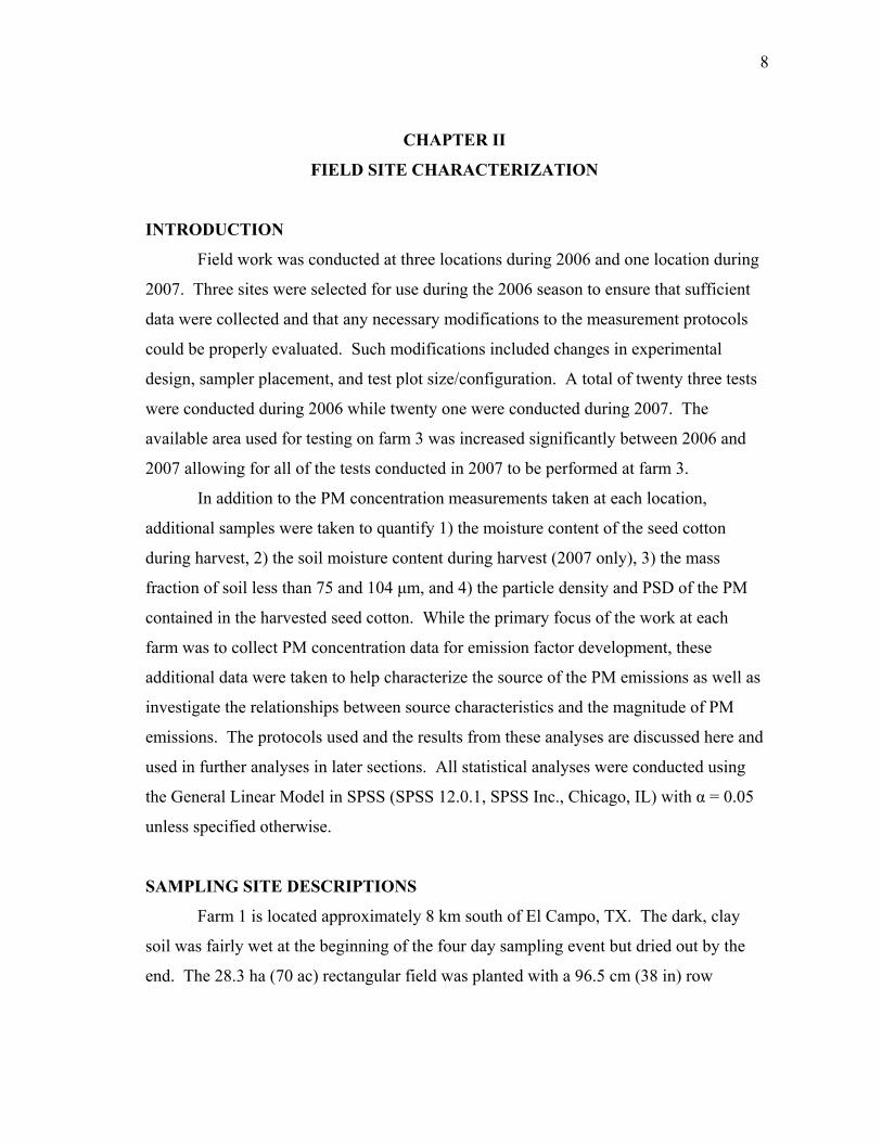
Farm 2 is located approximately 21 km south-southwest of College Station, TX.
The soils varied across the farm from clay to sandy clay loam. The soil was dry during
the four day sampling event. The rectangular 32.4 ha (80 ac) field is oriented in a
northeast-southwest manner with rows oriented northwest-southeast (96.5 cm row
spacing). The field was subdivided into nine 1.9 ha (4.7 ac) test plots, each with 366 m
row length (figure 3). DP555 BG/RR (Delta and Pine Land Company, Scott, MS) was
grown on farm 2 and Def® and Prep® (Bayer Crop Science, Research Triangle Park,
NC) were used to defoliate the crop and open the bolls.
Figure 3. Layout of the test plots used in the tests conducted on farm 2.
9
7
8
3
2
1
6
5
4
N

12
Nine total tests were planned for farm 2. Equipment malfunctions and the labor
intensive nature of the work again caused a reduction in the number of tests conducted to
eight. The experimental design was modified from that used at farm 1 to a randomized
complete block design with blocks on location within the field. This change in the
experimental design was made to account for differences in soil type within the field and
to reduce the labor involved with installing and removing the source sampling
equipment between tests. The test plots were ordered sequentially from northeast to
southwest and three groups of adjacent test plots were formed (area 1 = plots 1-3, area 2
= plots 4-6, area 3 = plots 7-9). The treatments were randomly assigned to one plot
within each area of the field and all of the plots for one treatment were harvested before
proceeding to the next treatment. The design of the experiments conducted at farm 2 is
shown in Table 2.
The experimental design to block by location within the field was modified due
to equipment failures and the labor intensive nature of the work. Again, the emission
factor results from farm 2 were analyzed for differences by treatment mean in SPSS.
Table 2. Design of the experiments conducted at farm 2.
Test No. Treatment Plot No.
Area No. (Experimental
Block)
Day of Test
1 6 Row 1 1 1 2 6 Row 5 2 1 3 6 Row 7 3 2 4 2 Row 2 1 2 5 2 Row 4 2 2 6 2 Row 8 3 3 7 6 Row w/SS 3 1 3 8 6 Row w/SS 6 2 3
13
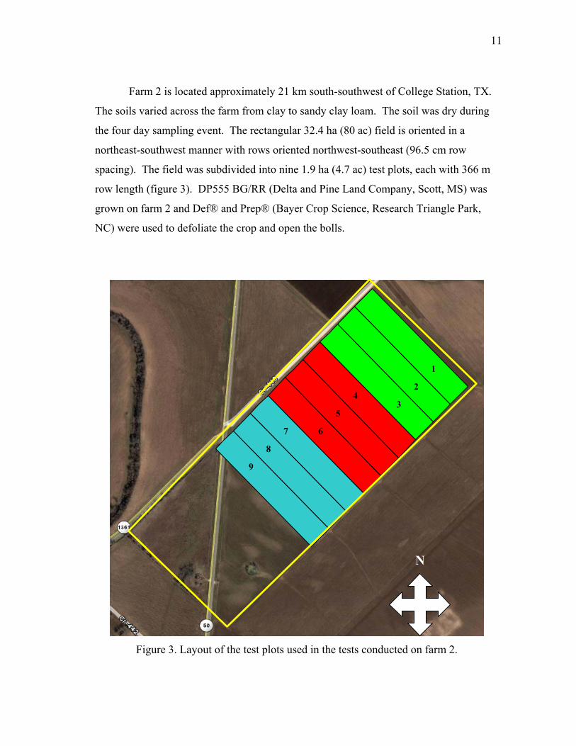
Farm 3 is located approximately 12.5 km southwest of College Station, TX. The
northeastern edge of the field is bordered by the Brazos River. The soil varies across the
field from clay to sand and remained dry during the 2006 sampling event. The rows
were spaced 101.6 cm (40 in) apart and oriented northeast to southwest. In 2006, the
13.8 ha (35 ac) field was subdivided into six test plots with areas ranging from 2 to 2.6
ha (4.9 to 6.9 ac) (see Figure 4). The row lengths of the test plots ranged from 184 to
300 m. FM988 LL/B2 was grown and defoliated with one treatment of Ginstar® and
Dropp® (Bayer Crop Science, Research Triangle Park, NC).
Figure 4. Layout of test plots on farm 3.
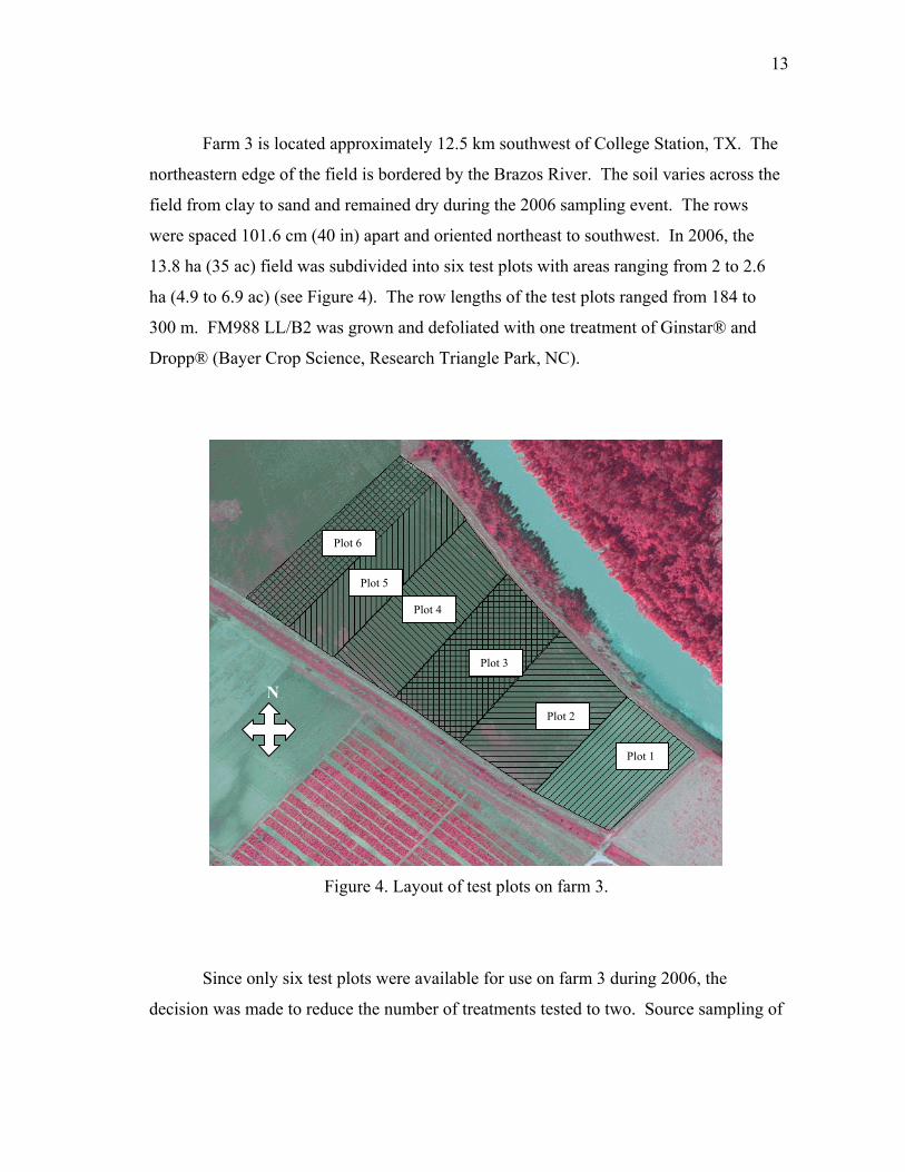
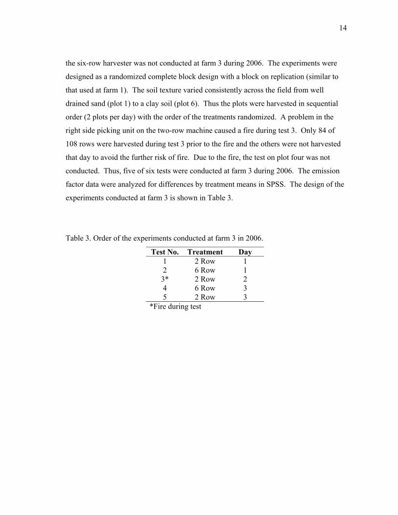
Since only six test plots were available for use on farm 3 during 2006, the
decision was made to reduce the number of treatments tested to two. Source sampling of
Plot 6
Plot 5
Plot 4
Plot 3
Plot 2
Plot 1
N
14
the six-row harvester was not conducted at farm 3 during 2006. The experiments were
designed as a randomized complete block design with a block on replication (similar to
that used at farm 1). The soil texture varied consistently across the field from well
drained sand (plot 1) to a clay soil (plot 6). Thus the plots were harvested in sequential
order (2 plots per day) with the order of the treatments randomized. A problem in the
right side picking unit on the two-row machine caused a fire during test 3. Only 84 of
108 rows were harvested during test 3 prior to the fire and the others were not harvested
that day to avoid the further risk of fire. Due to the fire, the test on plot four was not
conducted. Thus, five of six tests were conducted at farm 3 during 2006. The emission
factor data were analyzed for differences by treatment means in SPSS. The design of the
experiments conducted at farm 3 is shown in Table 3.
Table 3. Order of the experiments conducted at farm 3 in 2006.
Test No. Treatment Day 1 2 Row 1 2 6 Row 1 3* 2 Row 2 4 6 Row 3 5 2 Row 3
*Fire during test
15
The area available for testing on farm 3 in 2007 was more than double the area
available during 2006. Approximately 36 ha (90 ac) were planted to DP 455 BG/RR
(Delta and Pine Land Company, Scott, MS) and defoliated with one application of
Prep® and Ginstar® (Bayer Crop Science, Research Triangle Park, NC). The field was
planted with the same orientation and spacing as the 2006 crop. Twenty one test plots
were setup on farm 3 during 2007 as shown in Figure 5 and all three machine
configuration treatments were tested. To accommodate the research needs of other
scientists, the field was harvested in two phases. In phase one the 6-Row and 6-Row
w/SS treatments were randomly assigned to plots 1 – 15 and each of the plots assigned
to one treatment were harvested in sequential order before moving to the next treatment.
Weather conditions (rain) delayed the tests conducted with the two-row machine (phase
2) by approximately one week from the end of the five day sampling event with the six-
row machine. The two-row harvester tests were conducted in sequential order by plot
number on plots 16 – 21 over a three day period. The order of the experiments
conducted on farm 3 during 2007 is shown in Table 4. Heavy rainfall during the
growing season and limited applications of plant growth regulator resulted in extremely
tall and rank crop conditions at harvest. Thus more plant and organic material was
processed through the picking units during the harvest tests conducted on farm 3 during
2007.
The emission factor data collected from farm 3 during 2007 were analyzed for
treatment means in SPSS using ANOVA.

16
Figure 5. Aerial image of farm 3 showing the test plot layout used in 2007.
N

17
Table 4. Order of experiments conducted on farm 3 during 2007. Test Treatment Plot Day
1 6 Row 1 1 2 6 Row 4 2 3 6 Row 8 2 4 6 Row 9 2 5 6 Row 15 2 6 6 Row w/SS 2 3 7 6 Row w/SS 3 3 8 6 Row w/SS 5 4 9 6 Row w/SS 6 4 10 6 Row w/SS 7 4 11 6 Row w/SS 10 4 12 6 Row w/SS 11 4 13 6 Row w/SS 12 5 14 6 Row w/SS 13 5 15 6 Row w/SS 14 5 16 2 Row 16 6 17 2 Row 17 7 18 2 Row 18 7 19 2 Row 19 8 20 2 Row 20 8 21 2 Row 21 8
18
SAMPLING SITE CHARACTERIZATION METHODS
Seed Cotton Moisture Content Analysis
Seed cotton samples were hand harvested from each plot during each test
conducted in 2006 and 2007. The 100 g samples (approximate mass) were collected
from the plants and placed immediately in an air tight container for shipment back to the
laboratory for analysis. Each sample was analyzed to determine the moisture content at
harvest using the 10 hour oven method described by USDA (1972). The samples were
pre- and post-weighed on an analytical laboratory balance with 0.01 g resolution
(PB1502, Mettler-Toledo, Greifensee Switzerland). Accounting for the mass of the
sample container, the moisture content of each sample was determined by dividing the
net change in seed cotton mass by the initial mass of the seed cotton sample.
Seed Cotton Air Wash Analysis
Samples of harvested seed cotton were collected from the basket of the harvester
during each test in 2006 and 2007. Approximately 3 – 5 kg samples were collected and
placed in plastic bags for storage. The samples were collected for use in later air wash
analysis to provide PM samples for particle density analyses. Typically, the mass of PM
material collected on the filters used in the ground level TSP and PM10 samplers is not
sufficient to allow for particle density analysis. Approximately 1 g of material is needed
to perform an accurate particle density analysis on a sample of dust. The procedures
used to perform particle density analysis will be discussed in a later section.
The air washing process essentially removes PM from a sample of seed cotton by
pulling airflow through a sample container rotating inside a sealed enclosure. The
rotation of the sample container helps to separate the PM from the sample before it
passes through the mesh covering on the sample container and finally onto a collection
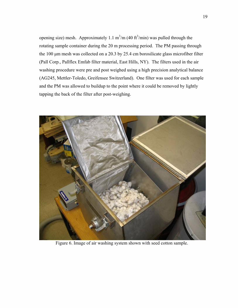
filter. The air washing machine used is shown in Figure 6. During each run with the air
wash machine, approximately 400 g of seed cotton was loaded into the inner sample
container and rotated at approximately 60 rpm. The side length dimension of the cubic
sample container is 0.304 m (1 ft) and each side was covered with 100 μm (nominal
19
opening size) mesh. Approximately 1.1 m3/m (40 ft3/min) was pulled through the
rotating sample container during the 20 m processing period. The PM passing through
the 100 μm mesh was collected on a 20.3 by 25.4 cm borosilicate glass microfiber filter
(Pall Corp., Pallflex Emfab filter material, East Hills, NY). The filters used in the air
washing procedure were pre and post weighed using a high precision analytical balance
(AG245, Mettler-Toledo, Greifensee Switzerland). One filter was used for each sample
and the PM was allowed to buildup to the point where it could be removed by lightly
tapping the back of the filter after post-weighing.
Figure 6. Image of air washing system shown with seed cotton sample.
20
The air washing process was used on the seed cotton samples collected in 2006
to provide material samples for particle density analysis. The resulting particle density
measurements were used to convert the PSD analysis results of the ground level TSP
sampler filters from an equivalent spherical diameter (ESD) basis to an aerodynamic
equivalent diameter (AED) basis. During 2007, the particle density samples used to
convert the PSD analysis results of the ground level TSP sampler filters from an ESD
basis to an AED basis were obtained by air washing the material captured in the source
sampler cyclone bucket.
Soil Sampling
Soil samples were collected from each test plot during 2006 and 2007. The
samples collected during 2006 were collected at the time the harvesting tests were
conducted and each sample consisted of approximately four to six 200 g sub-samples
collected from random points within each plot. During 2007, 31 samples were taken
across the 36 ha (90 ac) field in an evenly spaced grid pattern with approximately one
sampling point per ha. The 2007 samples were collected several weeks before harvest to
allow for ample processing time at the lab.
The soil samples collected in 2006 and 2007 were sieved to determine the mass
percent of soil less than 106 μm (#75 sieve) and less than 75 μm (#200 sieve). These
mass fractions were used for later correlation analysis with emission factor data to
investigate relationships by soil texture.
Each soil sample was processed through two sets of sieves for 20 min per set.
The designation of the sieves used are; set 1: 22.4 mm (7/8 in), 16 mm (5/8 in), 9.5 mm
(3/8 in), 8 mm (5/16 in), 2 mm (#10); and set 2: 1.4 mm (#14), 710 μm (#25), 180 μm
(#80), 106 μm (#140), and 75 μm (#200). The sieves were arranged in decreasing
opening size from top to bottom. The net material mass remaining in each sieve was
used to determine the mass percent of the original soil sample mass within each size
range. The procedure used to sieve the soil samples is described in greater detail in
Appendix A.

21
Soil Moisture Content Measurements
Surface soil moisture content measurements (top 10 cm) were conducted on farm
3 during the 2007 sampling events. Ten sampling sites were randomly located within
each test plot and the measurements were taken during the time of each test. Volumetric
soil moisture content measurements were taken using a hand held moisture meter (HH2,
Delta-T Devices, Cambridge England) with integrated soil probe (Theta Probe type
ML2x, Delta-T Devices, Cambridge England). Volumetric soil moisture content is
equivalent to the volume of water present in the sample divided by the total volume of
the sample (soil + water) expressed as a percentage. The average soil moisture content
readings from each test were used in later correlation analysis with emission factor data.
RESULTS
Seed Cotton Moisture Content Analysis
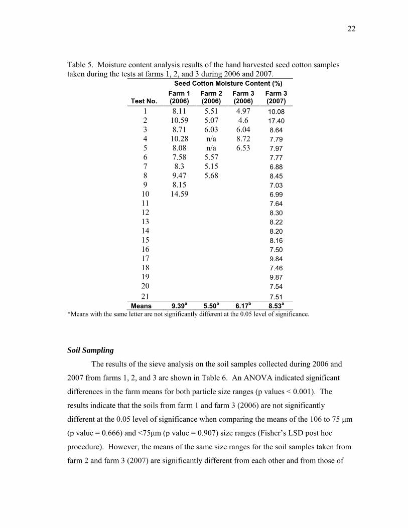
The moisture content analysis results of the hand harvested seed cotton samples
taken during the tests conducted at farms 1, 2, and 3 in 2006 and 2007 are shown in
Table 5. Combining the data for both years, means by farm and harvesting treatment
were compared using analysis of variance (ANOVA) with Fisher’s Least Significant
Difference (LSD) post hoc procedure (due to unequal sample sizes) with α = 0.05.
The results of the analysis indicate that there was no significant difference
between the seed cotton moisture content values by harvester treatment (p value =
0.467). However, significant differences were observed between the farm average
moisture content values (p value = 0.001). The mean seed cotton moisture content
values for farm 1 and farm 3 (2007) were significantly higher than the means for farm 2
and farm 3 (2006) as indicated in Table 5. This result is likely a consequence of the high
relative humidity encountered during the sampling events at farm 1 and also due to the
rank condition of the cotton at farm 3 during 2007.
22
Table 5. Moisture content analysis results of the hand harvested seed cotton samples taken during the tests at farms 1, 2, and 3 during 2006 and 2007.
Seed Cotton Moisture Content (%)
Test No. Farm 1 (2006)
Farm 2 (2006)
Farm 3 (2006)
Farm 3 (2007)
1 8.11 5.51 4.97 10.08 2 10.59 5.07 4.6 17.40 3 8.71 6.03 6.04 8.64 4 10.28 n/a 8.72 7.79 5 8.08 n/a 6.53 7.97 6 7.58 5.57 7.77 7 8.3 5.15 6.88 8 9.47 5.68 8.45 9 8.15 7.03 10 14.59 6.99 11 7.64 12 8.30 13 8.22 14 8.20 15 8.16 16 7.50 17 9.84 18 7.46 19 9.87 20 7.54 21 7.51
Means 9.39a 5.50b 6.17b 8.53a *Means with the same letter are not significantly different at the 0.05 level of significance.
Soil Sampling
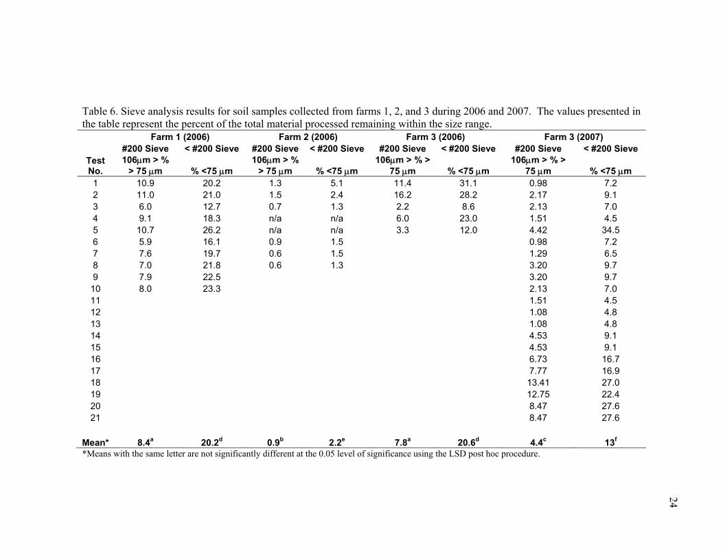
The results of the sieve analysis on the soil samples collected during 2006 and
2007 from farms 1, 2, and 3 are shown in Table 6. An ANOVA indicated significant
differences in the farm means for both particle size ranges (p values < 0.001). The
results indicate that the soils from farm 1 and farm 3 (2006) are not significantly
different at the 0.05 level of significance when comparing the means of the 106 to 75 μm
(p value = 0.666) and <75μm (p value = 0.907) size ranges (Fisher’s LSD post hoc
procedure). However, the means of the same size ranges for the soil samples taken from
farm 2 and farm 3 (2007) are significantly different from each other and from those of

23
farm 1 and 3 (2006) at the 0.05 level of significance. Further analysis indicates that
significant differences exist between the harvesting treatment means within the 106 to 75
μm (p value = 0.666) and <75μm (p value = 0.907) size ranges (Fisher’s LSD post hoc
procedure).
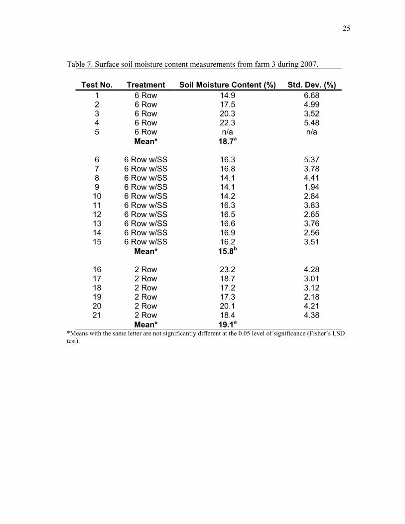
Soil Moisture Content Measurements
Soil moisture content measurements were conducted during 2007 at farm 3 to
investigate potential trends of increasing PM emissions with decreasing surface soil
moisture content. An ANOVA on the soil moisture content data indicates that
significant differences did exist between the mean soil moisture content values of the
plots by harvesting treatment (p value = 0.009). LSD post hoc tests indicate that the
mean plot soil moisture content for the 6-row and 2-row harvesting treatments were not
significantly different (p value = 0.764). However, there was a significant difference in
the mean soil moisture content between the 6-row w/SS and 6-row treatments (p value =
0.025) and between the 6-row w/SS and 2-row treatments (p value = 0.005). These
results were expected as the 6-row w/SS tests were conducted one day after the 6-row
harvesting treatment tests. A rain event occurred the same day that the 6-row w/SS tests
were finished and the 2-row tests were not conducted for approximately one week to
allow for sufficient drying time. The results of the surface soil content measurements
are presented in Table 7.
24
Table 6. Sieve analysis results for soil samples collected from farms 1, 2, and 3 during 2006 and 2007. The values presented in the table represent the percent of the total material processed remaining within the size range. Farm 1 (2006) Farm 2 (2006) Farm 3 (2006) Farm 3 (2007) #200 Sieve < #200 Sieve #200 Sieve < #200 Sieve #200 Sieve < #200 Sieve #200 Sieve < #200 Sieve Test No.
106μm > % > 75 μm % <75 μm
106μm > % > 75 μm % <75 μm
106μm > % > 75 μm % <75 μm
106μm > % > 75 μm % <75 μm
1 10.9 20.2 1.3 5.1 11.4 31.1 0.98 7.2 2 11.0 21.0 1.5 2.4 16.2 28.2 2.17 9.1 3 6.0 12.7 0.7 1.3 2.2 8.6 2.13 7.0 4 9.1 18.3 n/a n/a 6.0 23.0 1.51 4.5 5 10.7 26.2 n/a n/a 3.3 12.0 4.42 34.5 6 5.9 16.1 0.9 1.5 0.98 7.2 7 7.6 19.7 0.6 1.5 1.29 6.5 8 7.0 21.8 0.6 1.3 3.20 9.7 9 7.9 22.5 3.20 9.7 10 8.0 23.3 2.13 7.0 11 1.51 4.5 12 1.08 4.8 13 1.08 4.8 14 4.53 9.1 15 4.53 9.1 16 6.73 16.7 17 7.77 16.9 18 13.41 27.0 19 12.75 22.4 20 8.47 27.6 21 8.47 27.6
Mean* 8.4a 20.2d 0.9b 2.2e 7.8a 20.6d 4.4c 13f *Means with the same letter are not significantly different at the 0.05 level of significance using the LSD post hoc procedure.
25
Table 7. Surface soil moisture content measurements from farm 3 during 2007.
Test No. Treatment Soil Moisture Content (%) Std. Dev. (%) 1 6 Row 14.9 6.68 2 6 Row 17.5 4.99 3 6 Row 20.3 3.52 4 6 Row 22.3 5.48 5 6 Row n/a n/a Mean* 18.7a 6 6 Row w/SS 16.3 5.37 7 6 Row w/SS 16.8 3.78 8 6 Row w/SS 14.1 4.41 9 6 Row w/SS 14.1 1.94
10 6 Row w/SS 14.2 2.84 11 6 Row w/SS 16.3 3.83 12 6 Row w/SS 16.5 2.65 13 6 Row w/SS 16.6 3.76 14 6 Row w/SS 16.9 2.56 15 6 Row w/SS 16.2 3.51 Mean* 15.8b
16 2 Row 23.2 4.28 17 2 Row 18.7 3.01 18 2 Row 17.2 3.12 19 2 Row 17.3 2.18 20 2 Row 20.1 4.21 21 2 Row 18.4 4.38
Mean* 19.1a *Means with the same letter are not significantly different at the 0.05 level of significance (Fisher’s LSD test).
26
CHAPTER III
EMISSION FACTOR DEVELOPMENT PROTOCOL I:
UPWIND/DOWNWIND SAMPLING WITH DISPERSION MODELING
INTRODUCTION
Emission factors for most stationary sources can be developed through source
measurement techniques. Often times these source measurements are conducted using
EPA approved sampling devices and methods such as the EPA method 5, EPA method
201a, or CTM-039 stack samplers for measuring TSP, PM10, or PM2.5 emission
concentrations, respectively (CFR, 2007 ). The resulting emission concentrations can be
converted to emission rates by multiplying by the gas flow rate in the exhaust stream and
finally to emission factors by normalizing the emission rates to a production unit basis.
However, agricultural operations such as feedlots, dairies, and many field operations are
not stationary sources with common points of pollutant emission which can be easily
measured on a source basis. Emission factors for these fugitive sources have been
developed through back-calculating emission fluxes with a dispersion model and
simultaneously collected concentration and meteorological data (Goodrich, 2006;
Parnell, 1994; Wanjura et. al. 2004).
The EPA recommended dispersion model for regulatory use was ISCST3 until
2006 when EPA began promoting the use of AERMOD (Federal Register, 2005).
According to EPA (Federal Register, 2005), all state air pollution regulatory agencies
had a one year transition period during 2007 in which to make the switch from ISCST3
to AERMOD. The EPA regulatory platform for near-field modeling has remained
fundamentally unchanged over the last 25 years with ISCST3 selected as the workhorse
model for regulatory use (EPA, 2004).
“The objective of the AMS/EPA Regulatory Model Improvement Committee (AERMIC) was to develop a replacement for the ISC3 model by: 1)adopting ISCST3’s input/output computer architecture, 2) updating, where practical, antiquated ISC3 model algorithms with newly developed or current state-of-the-art modeling techniques, and 3)insuring that the source and atmospheric

27
processes presently modeled by ISC3 will continue to be handled by the AERMIC Model (AERMOD), albeit in an improved manner”. (EPA, 2004)
Dispersion models are used in the air pollution regulatory process to predict
downwind concentrations from a source with a given emission factor and meteorological
data. These concentration results are used in the preparation of State Implementation
Plans (SIP), new source permits, risk assessments and exposure analysis for toxic air
pollutants (EPA, 2004). Thus, appropriate emission factors must be used in the
modeling process to estimate downwind concentration impacts of a source so to not
preclude the equitable regulation of the source. Moreover, an emission factor
appropriate for ISCST3 may not be appropriate for use in AERMOD. Powell et al.
(2006) showed that fugitive emissions from an area source may be over-estimated by
AERMOD compared to ISCST3 when using the same emission factor and
meteorological conditions.
The methods presented in this protocol employ both ISCST3 and AERMOD to
produce emission factor estimates from the ground level concentration and
meteorological data collected during the 2006 and 2007 sampling events. The following
general steps are used to develop an emission factor according to this protocol:
1. Meteorological data measured onsite during each test is processed into the
proper formats required by the dispersion model and input to the model-user
interface program. The model-user interfaces used for ISCST3 and
AERMOD were BREEZE ISC GIS Pro (BREEZE ISC GIS Pro v. 5.2.1,
Trinity Consultants, Dallas, TX) and BREEZE AERMOD 6 (BREEZE
AERMOD v. 6.1.37, Trinity Consultants, Dallas, TX), respectively.
2. The user defines model setup parameters such as the size and orientation of
the area source, the emission release height, and receptor locations and
heights in the user-interface program. An area source release height of 4 m
and receptor heights of 2 m were used to model the harvesting operations with
flat terrain conditions. At this point the user also specifies an initial source
emission flux (Q1). The initial emission flux used in this work was 0.002569
28
g/m2-s. This value is equivalent to the PM10 emission factor used in
California of 1.9 kg/ha (1.7 lb/ac) under the following assumptions: 1) 101.6
cm (40 in) row spacing, 2) 6.4 km/hr (4 mph) harvester speed, 3) harvester
width of six rows, and 4) the mass fraction of TSP that is PM10 is 20%.
3. The user then runs the model to produce a set of model predicted
concentrations (C1) at each receptor location.
4. The Gaussian dispersion equation defines the relationship between downwind
concentration and source emission rate (flux) to be directly proportional such
that an increase in emission flux will produce a proportional increase in
estimated concentration. Thus, the initial area source flux (Q1), initial model
predicted concentration, and measured concentration (C2) for a particular
receptor location are used in equation 1 to determine the area source flux (Q2)
required by the dispersion model to predict the measured concentration value.
This process is repeated for each receptor location and the average of the Q2
values for the downwind receptor locations is reported as the test average.
2
1
2
1
CC
= (1)
5. Upwind samplers were used during 2006 and 2007 to measure background
PM concentrations at each site. In many cases, the upwind sampler
concentrations from 2006 were significantly influenced by outside sources
thus invalidating the background concentration measurement. Therefore, the
measured concentrations used in the dispersion modeling process for 2006
were not corrected to a net basis by subtracting the background concentration.
In effect, this provides a level of conservatism to the resulting emission
factors from 2006. This was not the case for 2007 as valid upwind
concentration measurements were used to correct the downwind
concentrations to a net basis.
6. The test average flux values are then converted to emission factors for size
range X (X indicating TSP, PM10, or PM2.5) according to equation 2.

29
CMFDQEF XPMtavgXPM *** ,, = (2)
where:
EFPM,X = PM emission factor for size range X, kg/ha (lb/ac),
Qavg = test average flux, g/m2-s,
Dt = test duration, min,
MFPM,X = mass fraction of PMX from PSD analysis (decimal), and
C = unit conversion constant, 600 for EF in kg/ha (535 for EF in lb/ac).
The concentrations used in the dispersion modeling process are TSP
measurements. PM10 and PM2.5 emission factors were determined by multiplying the
TSP emission factors by the respective mass fractions from PSD analysis. Buser et al.
(2001) showed that FRM PM10 and PM2.5 samplers report concentrations far in excess of
true concentrations when sampling PM with a mass median diameter larger than the
cutpoint of the sampler. Therefore, concentration measurement error imparted by the
sampler propagates directly through to emission factors developed through dispersion
modeling.
PARTICULATE MATTER CONCENTRATION MEASUREMENTS
Six sets of collocated low volume TSP and PM10 samplers were used to measure
the PM concentrations upwind and down wind of the harvesting operation during each
test during 2006. Five sets of collocated samplers were arranged around the test plots to
measure the PM concentrations downwind of the harvesting operation. One set of
collocated samplers was placed at a distance (100 – 200 m approximately) away from
the test plot to measure the background PM concentrations in the area. The common
sampler arrangement around the test plots is shown in Figure 7. This arrangement was
modified during tests 1 – 5 of farm 2 where the downwind samplers were all placed
inline along the downwind side of the test plot (Figure 8). This modification was made
to increase the number of samplers measuring the highest downwind concentrations
from the operation. The arrangement shown in Figure 4 was used to ensure that a

30
reliable downwind concentration would be measured from the harvesting operation in
times of meandering wind direction.
The sampler arrangement shown in Figure 7 was used again in 2007. However,
only four sets of collocated samplers were used along the east and west sides of each
plot. The northern most sampler location shown in Figure 4 was not used during 2007.
Figure 7. Typical arrangement of collocated TSP/PM10 samplers around the test plots.
Upwind Samplers
≈ 200 m
30 m
60 m
30 m
Test Plot
Wind
Downwind Samplers
10 m
Met Station
North
31
Figure 8. Modified sampler arrangement used during tests 1 – 5 at farm 2.
The TSP and PM10 samplers used to measure PM concentrations upwind and
downwind of the harvesting operations both operated with an air flow rate of 16.7 l/min
(Wanjura et. al., 2005b). The flow rate of the samplers used in this study is
approximately 85 times less than the flow rate of a comparable “high volume” federal
reference method (FRM) TSP or PM10 sampler (1.42 m3/min). Thus the term low
volume is used to describe the sampler air flow rate of the samplers used in this study.
The TSP inlet head used in this study was designed and evaluated by Wanjura et.
al. (2005b). TSP concentration measurements represent the concentration of a broad
range of inhaleable particles. The cutpoint of the TSP sampler was reported to be
around 45 μm with a slope of 1.5 by McFarland and Ortiz (1983). Thus the TSP sampler
concentration represents the concentration of airborne particles with diameters up to 100
μm. The results of subsequent PSD analysis of the PM captured on the TSP sampler
Upwind Samplers
≈ 200 m
30 m
30 m
Test Plot
Wind
Downwind Samplers
Met Station
North
32
filter was used to determine the true concentration of PM less than a given particle
diameter (i.e. true PM10 or PM2.5 concentrations) (Buser, 2004).
The PM10 samplers used the Graseby-Andersen FRM PM10 inlet. The
concentrations measured by the PM10 samplers are intended to represent the
concentration of PM less than 10 μm. However, the concentrations measured by the
FRM PM10 samplers do not accurately represent true PM10 concentrations when
sampling PM from agricultural operations due to the interaction between the sampler
performance characteristics and the PSD of the sampled PM (Buser, 2004). PM10
concentration measurements were made in this study using FRM PM10 samplers to
investigate this sampling error phenomenon in the presence of dust emitted from cotton
harvesting operations.
The systems used to establish and control the flow rate of the TSP and PM10
samplers were identical. The flow system used a 0.09 kW (1/8 hp) diaphragm pump
(917CA18-59, Thomas Industries, Sheboygan, WI) to draw the 16.7 l/min sample flow
rate through the sampler inlet head. Electrical power for the samplers was supplied by
gasoline powered generators located between the samplers. The air flow rate was
measured using a sharp edge orifice meter. The diameter of the orifice was 4.76 mm
(3/16 inch). The pressure drop across the orifice plate was measured by a Magnehelic
gauge (as a visual check) and also by a differential pressure transducer (PX274, Omega
Engineering, Inc., Stamford, Conn.). The differential pressure transducer converted the
differential pressure readings into a current (ma) signal that was recorded by a data
logger (HOBO H8 RH/Temp/2x External, Onset Computer Corp, Pocasset, MA).
Pressure drop readings were recorded for each sampler at the beginning and end of each
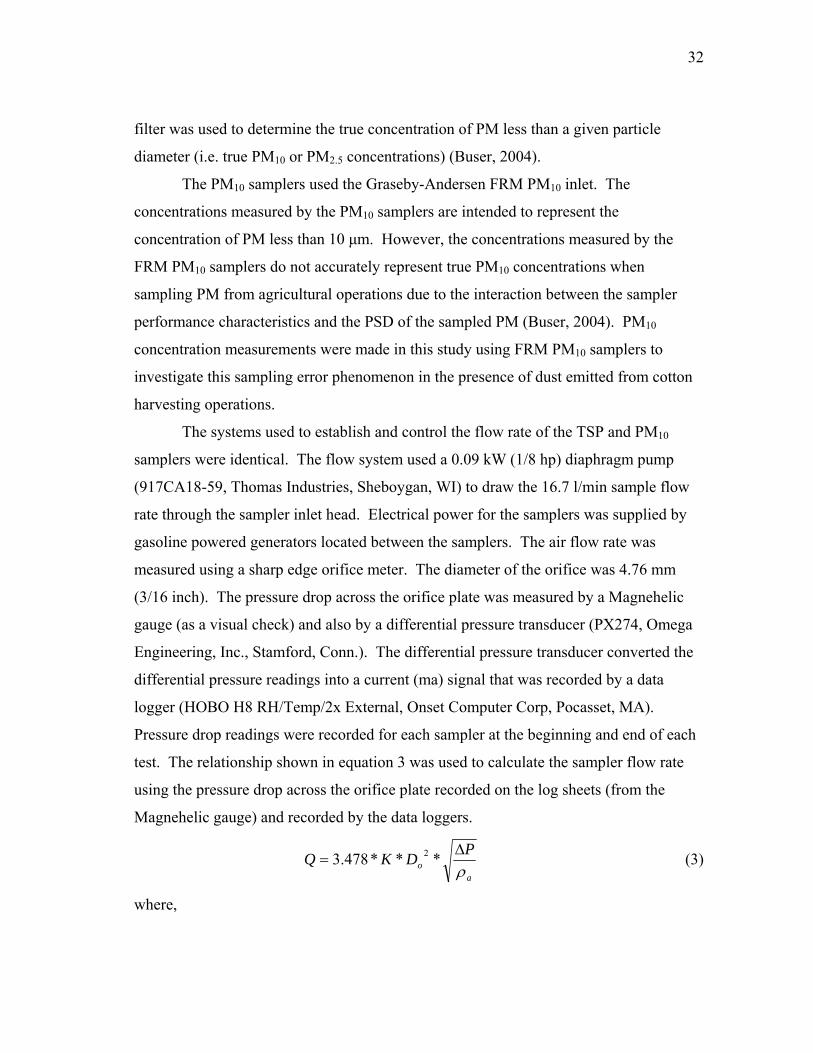
test. The relationship shown in equation 3 was used to calculate the sampler flow rate
using the pressure drop across the orifice plate recorded on the log sheets (from the
Magnehelic gauge) and recorded by the data loggers.
a
oPDKQ
ρΔ
= ***478.3 2 (3)
where,
33
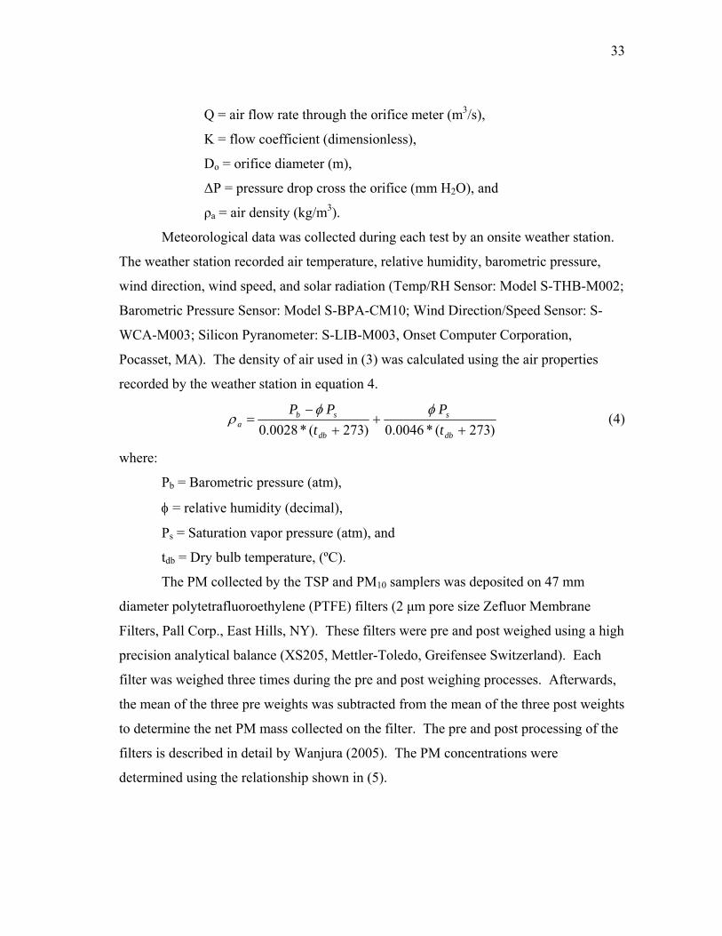
Q = air flow rate through the orifice meter (m3/s),
K = flow coefficient (dimensionless),
Do = orifice diameter (m),
ΔP = pressure drop cross the orifice (mm H2O), and
ρa = air density (kg/m3).
Meteorological data was collected during each test by an onsite weather station.
The weather station recorded air temperature, relative humidity, barometric pressure,
wind direction, wind speed, and solar radiation (Temp/RH Sensor: Model S-THB-M002;
Barometric Pressure Sensor: Model S-BPA-CM10; Wind Direction/Speed Sensor: S-
WCA-M003; Silicon Pyranometer: S-LIB-M003, Onset Computer Corporation,
Pocasset, MA). The density of air used in (3) was calculated using the air properties
recorded by the weather station in equation 4.
)273(*0046.0)273(*0028.0 ++
+−
=db
s
db
sba t
Pt
PP φφρ (4)
where:
Pb = Barometric pressure (atm),
φ = relative humidity (decimal),
Ps = Saturation vapor pressure (atm), and
tdb = Dry bulb temperature, (ºC).
The PM collected by the TSP and PM10 samplers was deposited on 47 mm
diameter polytetrafluoroethylene (PTFE) filters (2 μm pore size Zefluor Membrane
Filters, Pall Corp., East Hills, NY). These filters were pre and post weighed using a high
precision analytical balance (XS205, Mettler-Toledo, Greifensee Switzerland). Each
filter was weighed three times during the pre and post weighing processes. Afterwards,
the mean of the three pre weights was subtracted from the mean of the three post weights
to determine the net PM mass collected on the filter. The pre and post processing of the
filters is described in detail by Wanjura (2005). The PM concentrations were
determined using the relationship shown in (5).

34
∑Δ
=
iii tQ
MC (5)
where:
C = average concentration of PM measured over the test duration (μg/m3),
ΔM = change in mass of the filter due to PM loading (μg),
Qi = average air flow rate over the ith time interval, and
ti = ith time interval duration (s).
The logging intervals (ti) used by the data loggers was 12 s during 2006 and 1
min during 2007. However, when determining the total flow volume measured during
the test period using the beginning and ending pressure drop readings from the log
sheets, the time interval duration (ti) was the total duration of the test.
The total uncertainty due to systematic effects of the low volume sampling
systems was determined to be 11.85% by Price (2004) using the method described by
Kline and McClintock (1953).
DISPERSION MODELING
Industrial Source Complex Short Term Version 3
ISCST3 is a Gaussian dispersion model that uses the normal (Gaussian)
distribution to describe the horizontal and vertical dispersion of a pollutant downwind
from the source (Wanjura et. al., 2005c). The pollutant concentration estimated by
ISCST3 at a downwind receptor is influenced by meteorological factors (wind direction,
wind speed, temperature, etc.), source emission characteristics (emission height,
emission temperature, emission velocity, etc.), and receptor characteristics (receptor
height and distance from source to receptor). ISCST3 is an EPA approved dispersion
model for evaluating the impact of emissions from a source on downwind
concentrations. SAPRAs have used ISCST3 in New Source Review permitting
processes to determine off property concentrations resulting from emissions from the
facility seeking the permit.
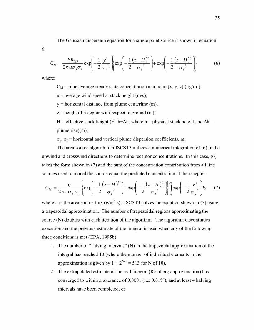
35
The Gaussian dispersion equation for a single point source is shown in equation
6.
( ) ( )⎪⎭
⎪⎬⎫
⎪⎩
⎪⎨⎧
⎟⎟⎠
⎞⎜⎜⎝
⎛ +−+⎟
⎟⎠
⎞⎜⎜⎝
⎛ −−⎟
⎟⎠
⎞⎜⎜⎝
⎛−= 2
2
2
2
2
2
21exp
21exp
21exp
2 zzyzy
TSPM
HzHzyu
ERC
σσσσσπ (6)
where:
CM = time average steady state concentration at a point (x, y, z) (µg/m3);
u = average wind speed at stack height (m/s);
y = horizontal distance from plume centerline (m);
z = height of receptor with respect to ground (m);
H = effective stack height (H=h+Δh, where h = physical stack height and Δh =
plume rise)(m);
σy, σz = horizontal and vertical plume dispersion coefficients, m.
The area source algorithm in ISCST3 utilizes a numerical integration of (6) in the
upwind and crosswind directions to determine receptor concentrations. In this case, (6)
takes the form shown in (7) and the sum of the concentration contribution from all line
sources used to model the source equal the predicted concentration at the receptor.
( ) ( ) dyyHzHzu
qCy
y yzzzyM ∫ ⎟
⎟⎠
⎞⎜⎜⎝
⎛−
⎪⎭
⎪⎬⎫
⎪⎩
⎪⎨⎧
⎟⎟⎠
⎞⎜⎜⎝
⎛ +−+⎟⎟
⎠
⎞⎜⎜⎝
⎛ −−=
2
1
2
2
2
2
2
2
21exp
21exp
21exp
2 σσσσσπ (7)
where q is the area source flux (g/m2-s). ISCST3 solves the equation shown in (7) using
a trapezoidal approximation. The number of trapezoidal regions approximating the
source (N) doubles with each iteration of the algorithm. The algorithm discontinues
execution and the previous estimate of the integral is used when any of the following
three conditions is met (EPA, 1995b):
1. The number of “halving intervals” (N) in the trapezoidal approximation of the
integral has reached 10 (where the number of individual elements in the
approximation is given by 1 + 2N-1 = 513 for N of 10),
2. The extrapolated estimate of the real integral (Romberg approximation) has
converged to within a tolerance of 0.0001 (i.e. 0.01%), and at least 4 halving
intervals have been completed, or

36
3. the extrapolated estimate of the real integral is less than 1.0 E-10, and at least 4
halving intervals have been completed.
The horizontal and vertical plume dispersion parameters, σy and σz, respectively,
are estimated in ISCST3 by the Pasquill-Gifford atmospheric stability parameter
estimates (Wanjura et al., 2005c). Beychok (1996) indicates that there is much
disagreement over the time period for which CM (equation 6) is the average
concentration when using Pasquill’s dispersion coefficients. He states further that some
argue that CM represents a 3 min concentration while others argue that C represents a 30
min concentration, but most will agree on a range of 10 – 15 min (Beychok, 1996).
When used for regulatory purposes, one hour average meteorological data is used in
ISCST3 to estimate downwind concentrations (EPA, 2000). Beychok (1996) indicates
that using one hour average meteorological data in ISCST3 can result in the over-
estimation of downwind concentrations by as much as 250%. Variations in wind
direction within a one hour period are not adequately accounted for in the use of hourly
average meteorological data (Fritz, 2002). Thus, the meteorological data collected
during each test was averaged using 15 – 20 minute intervals for use in ISCST3.
The meteorological data collected onsite during the tests was processed
according to the guidelines given by EPA (EPA, 2000).
o The meteorological data were processed using 15-20 minute averaging
times. 15 minute average meteorological data were used for the short
averaging period from farm 1 due to a weather station malfunction
whereas 20 minute average data were used for farms 2 and 3. It was
assumed that differences in the emission factors developed using the
short time average meteorological data (15 – 20 minute averages) would
not be a consequence of the 5 minute discrepancy in the averaging
periods.
o The wind direction was processed using the unit vector averaging
procedure described by EPA (2000).

37
o The wind speed data were scalar averaged over the two time periods
according to EPA recommendations.
o The Solar Radiation Delta-T (SRDT) method was used to define the
atmospheric stability classes during the tests. Solar radiation and wind
speed are the criteria used to define the atmospheric stability class
according to the SRDT method (EPA, 2000). Using these two criteria,
one can easily determine the day time atmospheric stability class using
the data in Table 8. Similarly, the wind speed and vertical temperature
gradient are used to classify night time atmospheric stability as presented
in Table 9.
Table 8. Key to Solar Radiation Delta – T method for estimating day time Pasquill-Gifford stability categories (EPA, 2000).
Day Time Solar Radiation (W/m2) Wind Speed (m/s) ≥925 925 - 675 675 - 175 <175
<2 1 1 2 4 2 - 3 1 2 3 4 3 - 5 2 2 3 4 5 - 6 3 3 4 4 ≥6 3 4 4 4
Table 9. Key to Solar Radiation Delta – T method for estimating night time Pasquill-Gifford stability categories (EPA, 2000).
Night Time Vertical Temperature Gradient Wind Speed (m/s) <0 ≥0
<2.0 5 6 2.0 - 2.5 4 5 ≥2.5 4 4

38
Emission flux values were calculated for each downwind sampler location for
each test. However, not all of the downwind sampler locations yielded reliable emission
flux values due to the orientation of the receptor to the source. For example, if the wind
direction were to shift such that the wind is blowing toward the northeast in Figure 4, the
northern and eastern samplers would become the downwind samplers. ISCST3 would
estimate the highest concentrations at the receptors located on the east side of the plot.
This is a consequence of the area within the source that is available to contribute to the
receptor concentration. If the concentrations measured during the test at the samplers
located along the north and eastern sides of the plot were approximately equal (this was
the situation in most cases), the resulting emission flux calculated for the sampler
located along the north side of the plot would be substantially larger than the fluxes
calculated for the samplers locates on the east side of the plot. Said differently, the
emission flux from the small area contributing to the concentration at the sampler
located on the north side of the plot would have to be much larger than the flux from the
larger areas contributing to the concentrations measured by the samplers on the east side
of the plot in order to calculate the same concentration at all three receptor locations. In
this situation, only two of the fluxes calculated from the downwind sampler
concentrations (the two located on the east side of the plot) would be used to determine
the average test flux.
AMS/EPA Regulatory Model: AERMOD
AERMOD is a steady state Gaussian dispersion model developed to model near
field dispersion of pollutants from stationary industrial sources. EPA (2004) states that
the major improvement in AERMOD over ISCST3 (which AERMOD is intended to
replace as the recommended regulatory model) is found in the incorporation of state-of-
the-art relationships for flow over complex terrain and in the ability to characterize the
planetary boundary layer (PBL) under both stable and convective conditions. For air
quality purposes, one is concerned with dispersion in the PBL. Garratt (1992) defines
the PBL as:

39
… the layer of air directly above the Earth’s surface in which the effects of the surface (friction, heating, and cooling) are felt directly on time scales less than a day, and in which significant fluxes of momentum, heat or matter are carried by turbulent motions on a scale of the order of the depth of the boundary layer or less.
The AERMOD model architecture is comprised of two preprocessors, AERMET
and AERMAP, which process standard meteorological data and terrain data,
respectively, and the AERMOD dispersion model. AERMAP is used to describe the
physical configuration of the model domain with regard to source-receptor orientation
(i.e. source elevation and release height and receptor elevation and height above grade).
AERMET is used to develop meteorological data files for use in AERMOD containing
standard meteorological data (surface measurements of wind speed, wind direction,
temperature, and cloud cover) as well as parameters to characterize the PBL such as
friction velocity (u*), Monin-Obukhov length (L), convective velocity scale (w*),
temperature scale (θ*), mixing height (zi), and surface heat flux (H). Estimates for
albedo, surface roughness, and Bowen ratio are also input to AERMET to help calculate
the PBL stability parameters. Similarity relationships are used in AERMOD with
meteorological data input files from AERMET to develop vertical profiles for wind
speed, lateral and turbulent fluctuations (σv, and σw respectively), potential temperature,
and potential temperature gradient (EPA, 2004). Detailed discussion on the methods
used in this work to develop the meteorological input files for AERMOD is given in the
following section.
The AERMOD dispersion model assumes the distributions of lateral and vertical
pollutant dispersion in the stable PBL (SBL) to be Gaussian. Further, the model
assumes that, in the convective PBL (CBL), the lateral distribution is Gaussian but the
vertical becomes a bi-Gaussian distribution (EPA, 2004). The vertical distribution of
pollutant dispersion in the CBL is skewed toward higher elevations above the ground
surface; meaning that higher pollutant concentrations are closer to the ground. While a
scrupulous description of the model formulation may be outside the scope of this work,
an abbreviated attempt will be made to describe the general formulation for stable and

40
convective conditions. A more in depth discussion of the model formulation is given in
EPA (2004).
Under both stable and convective conditions, the general form of the
concentration prediction equation is shown in (8). In both cases (convective and stable
conditions indicated by the c and s subscripts, respectively) the plume is contained in
two plume types; 1) the horizontal plume and 2) the terrain responding plume.
},,{)1(},,{},,{ ,, prrscrrrscrrrt zyxCfzyxCfzyxC −+= (8)
where Ct{xr, yr, zr} represents the total concentration predicted at receptor location xr, yr,
zr from the horizontal plume, Cc,s{xr, yr, zr}, and terrain following plume, Cc,s{xr, yr, zp}.
The horizontal and terrain following plumes are divided by a receptor specific dividing
streamline height, Hc. Hc is calculated for each receptor based on the receptor height
scale, hc, which describes the height of local terrain features which most dominate flow
in the region (EPA, 2004). The portion of the plume below Hc tends to remain in
horizontal flow (i.e. the horizontal plume) and is modeled such that when the plume
encounters a terrain feature such as a hill, it will either impact the hill surface or divide
and go around. The portion of the plume in the flow above Hc has sufficient kinetic
energy to sustain entrainment above the terrain surface; thus allowing the plume to
follow the terrain (EPA, 2004). The plume state weighting function, f, is the portion of
the total concentration from each plume type. The receptor height, zr, is referenced to
the stack base elevation and in cases of flat terrain, zr = zp and the equation reduces to a
single plume model dominated by the horizontal plume. Further, under convective
conditions, f = 0.5 and the concentration at a receptor with elevation above stack base
elevation is the average of the horizontal and terrain following plume concentrations
(EPA, 2004).
Under stable conditions, the point source dispersion equation takes the Gaussian
form shown in (9).
( ) ( )∑
∞
−∞= ⎥⎥⎦
⎤
⎢⎢⎣
⎡
⎟⎟⎠
⎞⎜⎜⎝
⎛ ++−+⎟
⎟⎠
⎞⎜⎜⎝
⎛ −−−=
m zs
ieffes
zs
ieffesy
zsrrs
zmhzzmhzF
uQzyxC 2
2
2
2
22
exp2
2exp
2},,{
σσσπ
(9)
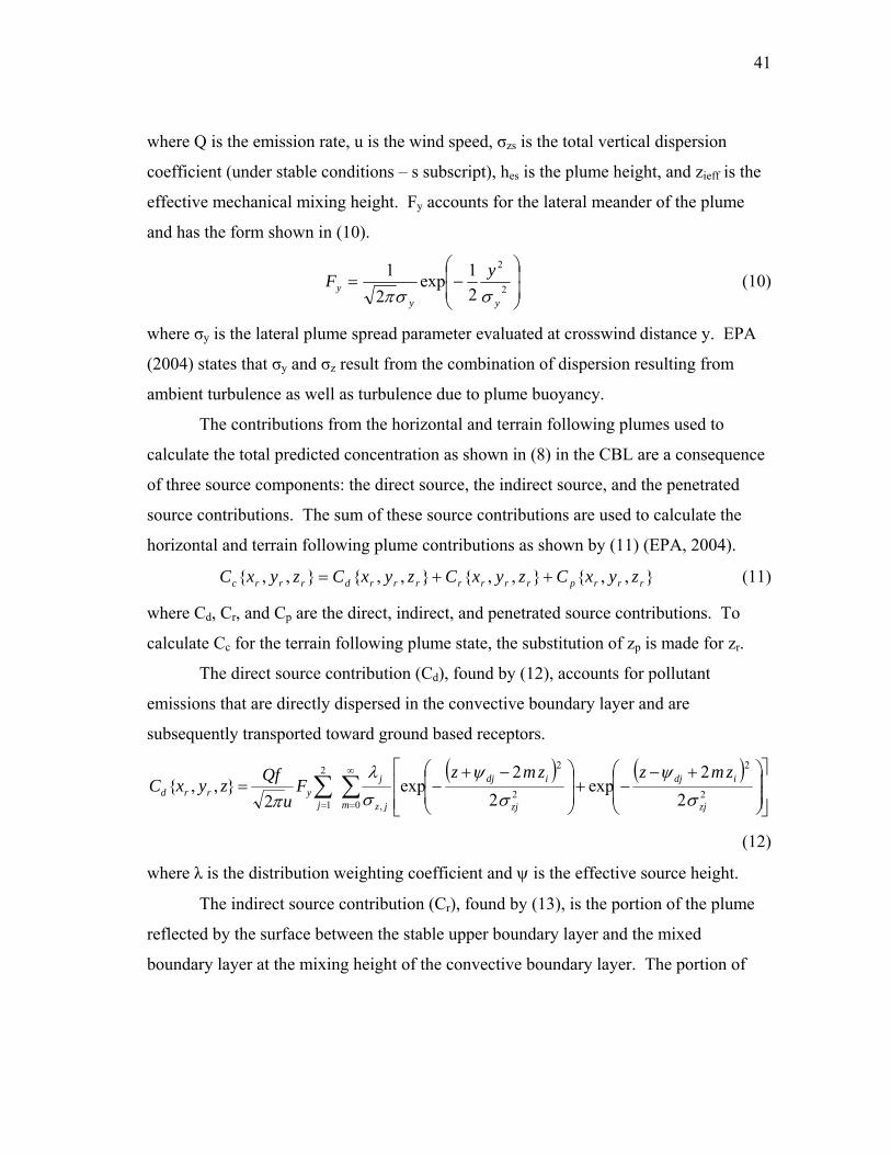
41
where Q is the emission rate, u is the wind speed, σzs is the total vertical dispersion
coefficient (under stable conditions – s subscript), hes is the plume height, and zieff is the
effective mechanical mixing height. Fy accounts for the lateral meander of the plume
and has the form shown in (10).
⎟⎟⎠
⎞⎜⎜⎝
⎛−= 2
2
21exp
21
yyy
yFσσπ
(10)
where σy is the lateral plume spread parameter evaluated at crosswind distance y. EPA
(2004) states that σy and σz result from the combination of dispersion resulting from
ambient turbulence as well as turbulence due to plume buoyancy.
The contributions from the horizontal and terrain following plumes used to
calculate the total predicted concentration as shown in (8) in the CBL are a consequence
of three source components: the direct source, the indirect source, and the penetrated
source contributions. The sum of these source contributions are used to calculate the
horizontal and terrain following plume contributions as shown by (11) (EPA, 2004).
},,{},,{},,{},,{ rrrprrrrrrrdrrrc zyxCzyxCzyxCzyxC ++= (11)
where Cd, Cr, and Cp are the direct, indirect, and penetrated source contributions. To
calculate Cc for the terrain following plume state, the substitution of zp is made for zr.
The direct source contribution (Cd), found by (12), accounts for pollutant
emissions that are directly dispersed in the convective boundary layer and are
subsequently transported toward ground based receptors.
( ) ( )∑∑
∞
== ⎥⎥⎦
⎤
⎢⎢⎣
⎡
⎟⎟
⎠
⎞
⎜⎜
⎝
⎛ +−−+
⎟⎟
⎠
⎞
⎜⎜
⎝
⎛ −+−=
02
2
2
2
,
2
1 22
exp2
2exp
2},,{
m zj
idj
zj
idj
jz
j
jyrrd
zmzzmzF
uQfzyxC
σψ
σψ
σλ
π
(12)
where λ is the distribution weighting coefficient and ψ is the effective source height.
The indirect source contribution (Cr), found by (13), is the portion of the plume
reflected by the surface between the stable upper boundary layer and the mixed
boundary layer at the mixing height of the convective boundary layer. The portion of

42
the indirect plume not reflected back toward the ground is assumed to penetrate to the
stable upper layer.
( ) ( )∑∑
∞
== ⎥⎥⎦
⎤
⎢⎢⎣
⎡
⎟⎟
⎠
⎞
⎜⎜
⎝
⎛ +−−+
⎟⎟
⎠
⎞
⎜⎜
⎝
⎛ −+−=
12
2
2
2
,
2
1 22
exp2
2exp
2},,{
m zj
irj
zj
irj
jz
j
jyrrr
zmzzmzF
uQfzyxC
σψ
σψ
σλ
π
(13)
The penetrated source contribution (Cp), found by (14), accounts for the portion
of the plume that initially penetrates the CBL above zi, and is subsequently re-entrained
by and dispersed in the CBL.
( ) ( )∑
∞
−∞= ⎥⎥⎦
⎤
⎢⎢⎣
⎡
⎟⎟⎠
⎞⎜⎜⎝
⎛ ++−+⎟
⎟⎠
⎞⎜⎜⎝
⎛ −−−
−=
m zp
ieffep
zp
ieffepy
zprrp
zmhzzmhzF
ufQzyxC 2
2
2
2
22
exp2
2exp
2)1(},,{
σσσπ
(14)
Meteorological Data Processing in AERMOD
The following discussions describe the methods used to calculate the
meteorological parameters used in AERMOD from meteorological data measured onsite
at farm 3 during 2007. Typically when creating the meteorological files for use in
AERMOD, one would obtain NWS or ADMS meteorological data files and process
them through the AERMOD meteorological data preprocessor AERMET. AERMET
calculates surface layer parameters from meteorological data collected from a particular
surface station location and user supplied surface estimates of albedo (r), surface
roughness (zo), and Bowen ratio (Bo). Empirical relationships encoded into the program
architecture of AERMET are then used to provide estimates for the variables required by
the dispersion relationships in AERMOD such as the Monin-Obukhov Length (L),
surface friction velocity (u*), surface sensible heat flux (H), and the convective scaling
velocity (w*). The final function of AERMET is to compile all of the measured, user
defined, and estimated meteorological data into the specific file formats required by
AERMOD. AERMOD requires two data files (which are output from the AERMET
preprocessor) to characterize the PBL conditions of the modeling domain: the surface
meteorological data file and the profile data file. The profile data file contains

43
information on the wind speed, direction, and temperature at a specified reference
height. While all of the data input to the AERMET preprocessor is passed through to
AERMOD, not all of the data is used by AERMOD. Specifically, the albedo, surface
sensible heat flux, and Bowen ratio are not used in any calculation performed by
AERMOD (Trinity Consultants, 2007).
AERMET was not used to develop the meteorological files used in AERMOD
for this work. Rather, the parameters estimated by AERMET were derived from
meteorological data measurements collected by an onsite weather station equipped with
3D and 2D sonic anemometers. These measurement derived parameters were then
incorporated into surface and profile files prepared by TCEQ for Burleson county from
1988 (TCEQ, 2007). These files were used to simplify the process of developing the
hourly meteorological files required by AERMOD. The 2D sonic anemometer
(WindSonic1, Gill Instruments Ltd., Lymington Hampshire) was used to measure the
wind speed and direction 3 m above the ground surface while the 3D sonic anemometer
(Model 81000, R.M. Young Co., Traverse City, MI) collected data for use in defining
the stability of the surface layer at 2m. Both the 2D and 3D sonic anemometers operated
with a sampling frequency of 4 Hz. Barometric pressure was measured by the weather
station with a barometric pressure sensor (Model 278, Setra Systems Inc., Boxborough,
MA) and temperature and relative humidity were measured by a T/RH probe mounted in
a solar radiation shield at 2 m (HMP50, Campbell Scientific Inc., Logan, UT). Net
radiation was also measured using two pyranometers, one mounted face up (CMP 22,
Kipp and Zonen, Delft, The Netherlands) and one mounted face down (CMP 6, Kipp and
Zonen, Delft, The Netherlands). The weather station sensor data was recorded by a data
logger (CR1000, Campbell Scientific Inc., Logan, UT) and stored on a removable
compact flash memory disk. The disk was changed between tests to simplify the data
processing work.
The data contained in the profile file from TCEQ (2007) was collected at a
reference height of 10 m. Wind data was not collected at 10 m during the 2007 tests on
farm 3. Rather, the information in the file from TCEQ was modified to reflect the wind
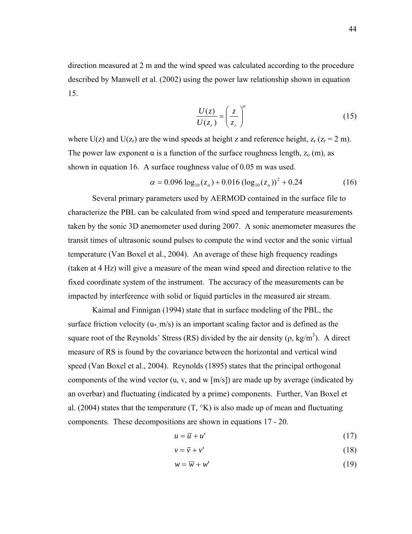
44
direction measured at 2 m and the wind speed was calculated according to the procedure
described by Manwell et al. (2002) using the power law relationship shown in equation
15. α
⎟⎟⎠
⎞⎜⎜⎝
⎛=
rr zz
zUzU
)()( (15)
where U(z) and U(zr) are the wind speeds at height z and reference height, zr (zr = 2 m).
The power law exponent α is a function of the surface roughness length, zo (m), as
shown in equation 16. A surface roughness value of 0.05 m was used.
24.0))((log016.0)(log096.0 21010 ++= oo zzα (16)
Several primary parameters used by AERMOD contained in the surface file to
characterize the PBL can be calculated from wind speed and temperature measurements
taken by the sonic 3D anemometer used during 2007. A sonic anemometer measures the
transit times of ultrasonic sound pulses to compute the wind vector and the sonic virtual
temperature (Van Boxel et al., 2004). An average of these high frequency readings
(taken at 4 Hz) will give a measure of the mean wind speed and direction relative to the
fixed coordinate system of the instrument. The accuracy of the measurements can be
impacted by interference with solid or liquid particles in the measured air stream.
Kaimal and Finnigan (1994) state that in surface modeling of the PBL, the
surface friction velocity (u*, m/s) is an important scaling factor and is defined as the
square root of the Reynolds’ Stress (RS) divided by the air density (ρ, kg/m3). A direct
measure of RS is found by the covariance between the horizontal and vertical wind
speed (Van Boxel et al., 2004). Reynolds (1895) states that the principal orthogonal
components of the wind vector (u, v, and w [m/s]) are made up by average (indicated by
an overbar) and fluctuating (indicated by a prime) components. Further, Van Boxel et
al. (2004) states that the temperature (T, °K) is also made up of mean and fluctuating
components. These decompositions are shown in equations 17 - 20.
'uuu += (17)
'vvv += (18)
'www += (19)

45
'TTT += (20)
The Reynolds’ stress and surface friction velocity are then calculated according
to equations 21 and 22, respectively.
''wuRS ρ−= (21)
( ) ( )222* '''' wvwuu += (22)
The friction velocity represents the horizontal shear stress exerted by the wind
vector on a horizontal surface (Van Boxel et al., 2004) and can be affected by
misalignment of the sonic anemometer with respect to a stream-wise coordinate system.
Slight misalignment of the instrument with respect to the vertical axis of the wind flow
vector can result in significant errors being introduced in to the calculation of the
covariance between the horizontal and vertical wind components (RS). The wind vector
changes slightly from one second to another while the anemometer is fixed to the
reference coordinate system it was configured to. If the wind vector tilts slightly
downward with respect to the instrument coordinate system, the slight perturbations in
the u and v directions will be interpreted as fluctuations in the w direction. While these
misinterpretations are small, they can contribute significantly to u’w’ and v’w’
(correlation between the horizontal and vertical wind speeds) (Van Boxel et al., 2004).
These errors can be precluded by performing a sequential three stage post measurement
rotation on the wind speed data collected by the sonic anemometer into a stream-wise
coordinate system. In this new reference frame, u is in the direction of the wind stream
lines (wind direction), v is in the plane of the wind stream lines and perpendicular to u,
and w is orthogonal to both u and v.
The first rotation (θ = yaw rotation angle, degrees) focuses the u direction of the
instrument into the wind direction. The second rotation (φ = pitch rotation, degrees)
orients u into the direction of the sloping stream lines and w perpendicular to u. The
final rotation orients v perpendicular to the surfaces of the wind streamlines and w
perpendicular to the streamline surfaces. A more detailed description of these rotations
is given by Van Boxel et al. (2004) with the mathematical rotations as shown here.
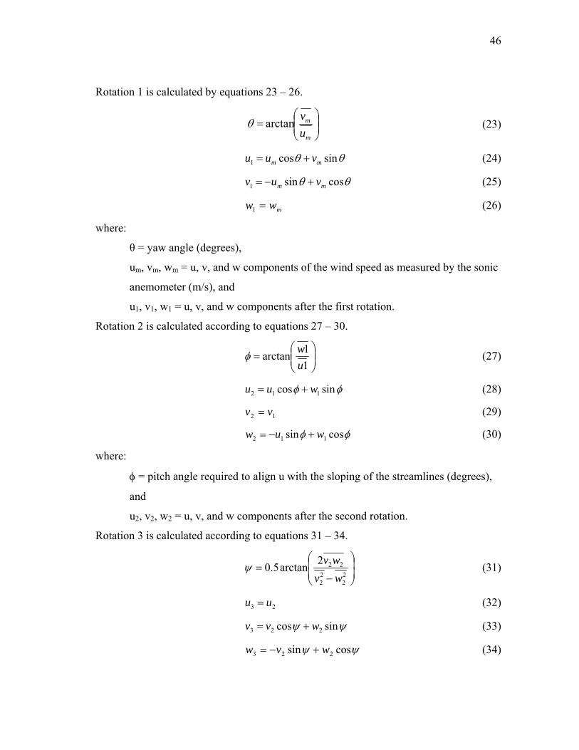
46
Rotation 1 is calculated by equations 23 – 26.
⎟⎟⎠
⎞⎜⎜⎝
⎛=
m
m
uvarctanθ (23)
θθ sincos1 mm vuu += (24)
θθ cossin1 mm vuv +−= (25)
mww =1 (26)
where:
θ = yaw angle (degrees),
um, vm, wm = u, v, and w components of the wind speed as measured by the sonic
anemometer (m/s), and
u1, v1, w1 = u, v, and w components after the first rotation.
Rotation 2 is calculated according to equations 27 – 30.
⎟⎟⎠
⎞⎜⎜⎝
⎛=
11arctan
uwφ (27)
φφ sincos 112 wuu += (28)
12 vv = (29)
φφ cossin 112 wuw +−= (30)
where:
φ = pitch angle required to align u with the sloping of the streamlines (degrees),
and
u2, v2, w2 = u, v, and w components after the second rotation.
Rotation 3 is calculated according to equations 31 – 34.
⎟⎟⎠
⎞⎜⎜⎝
⎛
−=
22
22
222arctan5.0wvwvψ (31)
23 uu = (32)
ψψ sincos 223 wvv += (33)
ψψ cossin 223 wvw +−= (34)
47
where:
ψ = rotation angle (degrees) required to orient v along the wind stream line
surfaces and w orthogonal to v and u, and
u3, v3, w3 = u, v, and w components after the third rotation.
The values for u, v, and w after the third rotation were used to calculate the mean
and fluctuating components of the wind vectors (equations 17 - 20) as well as the
correlations for calculating u*. The relationship for u* can be simplified to that shown in
equation 35 when the previous rotation is used to transform the measured data (Garratt,
1992).
( )''* wuu −= (35)
Along with the surface friction velocity, an estimate of the surface sensible heat
flux (H, W/m2) is needed to help characterize the PBL. The sensible heat flux can be
calculated using the correlation between the rotated vertical wind speed and temperature
(equation 36) (Etling, 1996).
''TwcH pρ= (36)
where cp is the specific heat of the air (J/kg-K). The PBL transitions from convective
(CBL) to stable conditions (SBL) when the sign of H changes from positive to negative.
The Monin-Obukhov length (L, m) is used to help define the thermal stability of
the PBL. The thermal stability parameter (ζ) is defined as Lz /−=ζ where z is the
measurement height of the sonic anemometer. The thermal stability parameter is
essentially a ratio of the thermal turbulence production to mechanical turbulence
production normalized by the dimensionless wind stress profile (Stull, 1988). The
Monin-Obukhov length was calculated by Hiscox et al. (2006) as shown in (37):
''
33
TwkguT
kgHuTc
L p ∗∗ −=
−=
ρ (37)
where k is the dimensionless von Karman constant (0.4) and g is the acceleration due to
gravity (9.81 m/s2).

48
The convective portion of turbulence in the PBL under convective conditions is
characterized in AERMOD by the convective velocity scale (w*, m/s). The convective
velocity scale is calculated as shown in equation 38. 3/1
⎟⎟⎠
⎞⎜⎜⎝
⎛=∗ Tc
gHzw
p
ic
ρ (38)
where zic is the convective mixing height (m).
Each hour of meteorological data input to AERMOD contains values for both the
convective and mechanical mixing height of the PBL. Ideally, the values for both the
convective and mechanical mixing heights (zim) would result from measurements taken
by upper air stations but can be calculated using the procedures described by EPA
(2004). The total depth of the PBL in AERMOD is determined based on the stability of
the atmosphere. In the CBL, the total depth of the PBL (zi) is taken as the maximum of
the mechanical or convective mixing heights. In the SBL, zi is defined by the
mechanical mixing height. Stability of the PBL is determined in AERMOD by the sign
of L; stable when L ≥ 0 and convective when L < 0.
The vertical potential temperature gradient in the 500 m above the PBL is
required by AERMOD to evaluate the potential for a buoyant plume to penetrate through
the PBL. Similar to the convective and mechanical mixing heights, measurements of the
vertical potential temperature gradient can be obtained from radiosondes of the upper
atmosphere. The values for the vertical potential temperature gradient were not expected
to significantly impact the near-field modeling results of this work and thus were
assumed to be equal to the values obtained in the meteorological data files from TCEQ.
Similarly, due to the lack of radiosonde data, the mechanical and convective mixing
heights used in this work were the historical data contained within the files obtained
from TCEQ.
The TCEQ recommends values for albedo, Bowen ratio, and surface roughness
for specific areas of the state to use in preparing meteorological data for use in
AERMOD (TCEQ, 2005). These values are included in the data input to AERMET to
use in the calculation of PBL stability parameters (EPA, 2004). However, in this case
49
the PBL parameters estimated using albedo and Bowen ratio values have been derived
from measured data. Thus, assumptions for albedo and Bowen ratio were not necessary
but a brief description of the parameters and recommended estimates is included.
The albedo value for an area describes the amount of incident solar radiation that
is reflected back from a surface (i.e. how bright the surface looks from above). The
albedo value required by AERMET is the noon day average. Typical values range from
0.1 for thick dense forest cover to 0.9 for a surface covered with fresh snow (TCEQ,
2005). A typical range albedo values recommended for the area of Texas near Burleson
county is 0.15 – 0.2 (TCEQ, 2005).
The Bowen ratio is another surface parameter used in the characterization of the
PBL to describe the amount of latent heat flux relative to the sensible heat flux at the
surface. Generally, the less moisture there is available for evaporation on a surface, the
higher the Bowen ratio. A moist surface typically has a low Bowen ratio. Typical
Bowen Ratio values recommended for the Burleson county area of Texas are on the
order of 0.6 (TCEQ, 2005). Both albedo and Bowen ratio are not used during night time
hours because of the lack of solar energy to drive CBL conditions at the surface of the
Earth.
Surface roughness varies with land use and terrain features. Typical values range
from 0.001 m over calm water to over 1 meter (or more) over a forest or urban area
(EPA, 2004). The TCEQ (2005) recommends that users select one of three ranges of
surface roughness values to use in AERMOD: low = 0.05 m, medium = 0.5 m, and high
= 1 m. The selection of the roughness parameter is dependent not only on the surface
characteristics of the source but also on the surrounding area. The medium surface
roughness value (zo = 0.5 m) was chosen since the source was made up by agricultural
crop land with medium sized plants and there was a line of trees approximately 10 m to
the north of the field with open flat fields to the south, east, and west.
The meteorological data collected onsite was processed to give hourly average
estimates of PBL parameters for use in AERMOD. Scalar averaging of surface wind
speed and unit vector averaging of surface wind direction measurements from the 2D

50
sonic anemometer were calculated according to the procedures described by EPA
(2000). The hourly met data calculated from the meteorological data collected during
the tests conducted at farm 3 during 2007 and used to modify the files obtained from
TCEQ is included in Appendix B.
Emission Factor Validation
Emission factors were calculated for each receptor location using ISCST3 with
the 2006 concentration data and both ISCST3 and AERMOD with the 2007 data. The
resulting emission factors spanned a wide range of values due to changing
meteorological conditions and the amount of relative source exposure at the receptor.
Thus it was necessary to validate the emission factors to exclude nonsensical values
from test average emission factor estimates. It is imperative at this point that objective
means are used to validate emission factors so not to bias the resulting emission factor
estimates. Therefore, the following process was used to identify receptors from which
reliable emission factor estimates could be obtained.
The first step in the validation process was to identify the downwind receptor
locations through the initial concentrations predicted by the dispersion model. The
downwind receptors are those which exhibit the highest net concentration predicted by
the dispersion model using the initial flux value and the meteorological data measured
onsite. Once the downwind receptors were identified, the following criteria were used to
ensure that 1) the sampling devices were operating appropriately, 2) the samplers were
not significantly influenced by an outside source of PM, and 3) the model algorithms
closely approximate the observed dispersion from the source as observed in the
measured concentration data.
1. Measured downwind sampler concentrations must be greater than the
concentrations measured by non-downwind samplers. Non-downwind
samplers are those which were intended to measure downwind concentrations
from the source but the wind direction precluded them from this
measurement. These are different from the upwind sampler in that the non-
51
downwind samplers could still measure a net positive concentration due to
other activity around the source generating PM (e.g. boll buggies, tractors,
small personnel vehicles, etc).
2. The ratio of the measured concentration for a receptor location to the sum of
the measured concentrations from all downwind receptors must approximate
the ratio of the predicted concentration at the receptor location to the sum of
the predicted concentrations at all downwind receptor locations. This
relationship is explained mathematically in equation 39.
∑∑≈
iiDWM
iDWM
iiDWS
iDWS
CC
CC
,,
,,
,,
,, (39)
where CS,DW,i is the concentration measured by a downwind (DW) sampler
(S) at location i and CM,DW,i is the concentration predicted by the dispersion
model (M) at downwind receptor location i. The emission factor from a
particular sampler/receptor location was considered suspect if the difference
between the measured and modeled ratios exceeded 0.25.
3. The ratio of the measured PM10 concentration to the measured TSP
concentration at a downwind sampler location must approximate the same
ratio for each downwind sampler location. This relationship is shown in
equation 40.
jTSPDW
jPMDW
iTSPDW
iPMDW
CC
CC
,,
,10,
,,
,10, ≈ (40)
for all i ≠ j where CDW,PM10,i is the measured PM10 concentration at downwind
receptor i. The calculated ratios for each downwind location were ranked and
a sampler concentration/emission factor was considered suspect if the
receptor ratio fell outside ±0.15 of the median ratio value. This ratio was also
calculated for the upwind samplers during each test to determine the ambient
PM10/TSP ratio. Thus the downwind sampler ratios were expected to be less
than the upwind sampler ratio as the PSD of the PM emitted from the
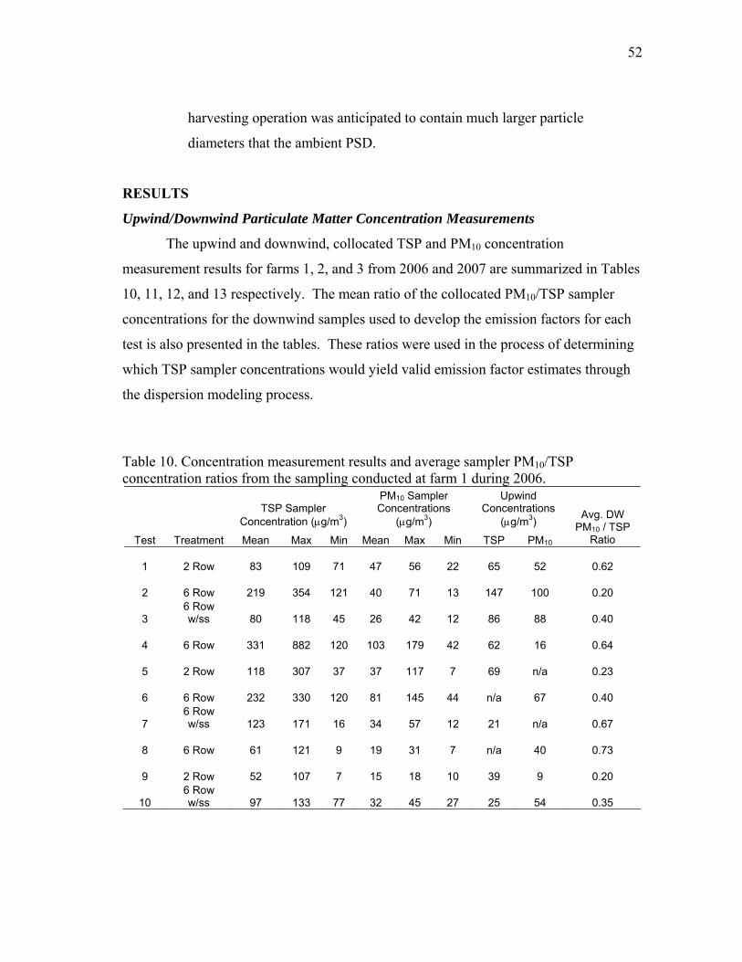
52
harvesting operation was anticipated to contain much larger particle
diameters that the ambient PSD.
RESULTS
Upwind/Downwind Particulate Matter Concentration Measurements
The upwind and downwind, collocated TSP and PM10 concentration
measurement results for farms 1, 2, and 3 from 2006 and 2007 are summarized in Tables
10, 11, 12, and 13 respectively. The mean ratio of the collocated PM10/TSP sampler
concentrations for the downwind samples used to develop the emission factors for each
test is also presented in the tables. These ratios were used in the process of determining
which TSP sampler concentrations would yield valid emission factor estimates through
the dispersion modeling process.
Table 10. Concentration measurement results and average sampler PM10/TSP concentration ratios from the sampling conducted at farm 1 during 2006.
TSP Sampler
Concentration (μg/m3)
PM10 Sampler Concentrations
(μg/m3)
Upwind Concentrations
(μg/m3)
Test Treatment Mean Max Min Mean Max Min TSP PM10
Avg. DW PM10 / TSP
Ratio
1 2 Row 83 109 71 47 56 22 65 52 0.62
2 6 Row 219 354 121 40 71 13 147 100 0.20
3 6 Row w/ss 80 118 45 26 42 12 86 88 0.40
4 6 Row 331 882 120 103 179 42 62 16 0.64
5 2 Row 118 307 37 37 117 7 69 n/a 0.23
6 6 Row 232 330 120 81 145 44 n/a 67 0.40
7 6 Row w/ss 123 171 16 34 57 12 21 n/a 0.67
8 6 Row 61 121 9 19 31 7 n/a 40 0.73
9 2 Row 52 107 7 15 18 10 39 9 0.20
10 6 Row w/ss 97 133 77 32 45 27 25 54 0.35
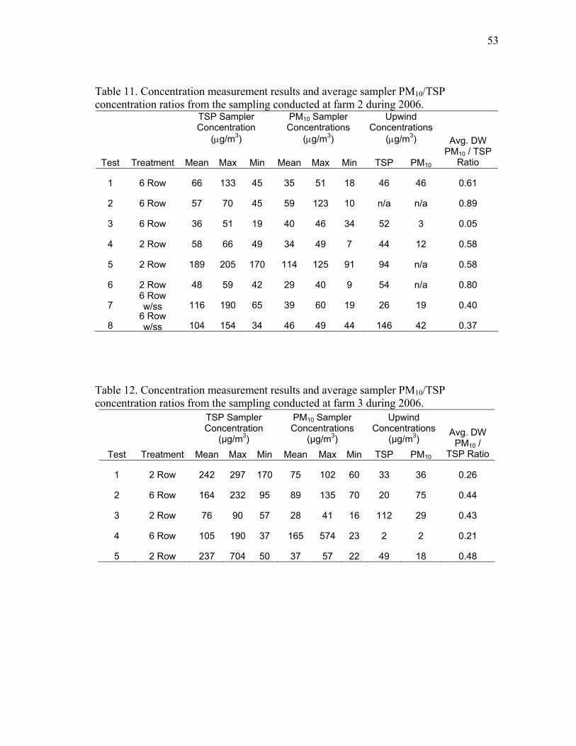
53
Table 11. Concentration measurement results and average sampler PM10/TSP concentration ratios from the sampling conducted at farm 2 during 2006.
TSP Sampler Concentration
(μg/m3)
PM10 Sampler Concentrations
(μg/m3)
Upwind Concentrations
(μg/m3)
Test Treatment Mean Max Min Mean Max Min TSP PM10
Avg. DW PM10 / TSP
Ratio
1 6 Row 66 133 45 35 51 18 46 46 0.61
2 6 Row 57 70 45 59 123 10 n/a n/a 0.89
3 6 Row 36 51 19 40 46 34 52 3 0.05
4 2 Row 58 66 49 34 49 7 44 12 0.58
5 2 Row 189 205 170 114 125 91 94 n/a 0.58
6 2 Row 48 59 42 29 40 9 54 n/a 0.80
7 6 Row w/ss 116 190 65 39 60 19 26 19 0.40
8 6 Row w/ss 104 154 34 46 49 44 146 42 0.37
Table 12. Concentration measurement results and average sampler PM10/TSP concentration ratios from the sampling conducted at farm 3 during 2006.
TSP Sampler Concentration
(μg/m3)
PM10 Sampler Concentrations
(μg/m3)
Upwind Concentrations
(μg/m3) Test Treatment Mean Max Min Mean Max Min TSP PM10
Avg. DW PM10 /
TSP Ratio
1 2 Row 242 297 170 75 102 60 33 36 0.26
2 6 Row 164 232 95 89 135 70 20 75 0.44
3 2 Row 76 90 57 28 41 16 112 29 0.43
4 6 Row 105 190 37 165 574 23 2 2 0.21
5 2 Row 237 704 50 37 57 22 49 18 0.48
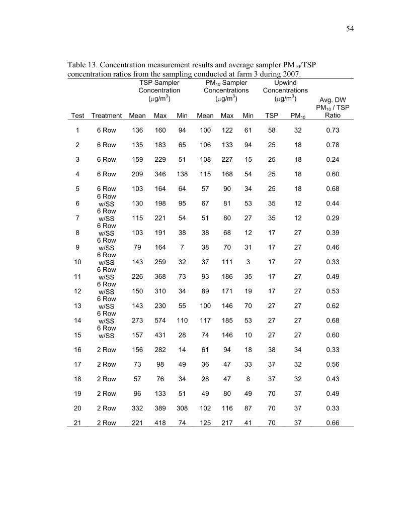
54
Table 13. Concentration measurement results and average sampler PM10/TSP concentration ratios from the sampling conducted at farm 3 during 2007.
TSP Sampler Concentration
(μg/m3)
PM10 Sampler Concentrations
(μg/m3)
Upwind Concentrations
(μg/m3)
Test Treatment Mean Max Min Mean Max Min TSP PM10
Avg. DW PM10 / TSP
Ratio
1 6 Row 136 160 94 100 122 61 58 32 0.73
2 6 Row 135 183 65 106 133 94 25 18 0.78
3 6 Row 159 229 51 108 227 15 25 18 0.24
4 6 Row 209 346 138 115 168 54 25 18 0.60
5 6 Row 103 164 64 57 90 34 25 18 0.68
6 6 Row w/SS 130 198 95 67 81 53 35 12 0.44
7 6 Row w/SS 115 221 54 51 80 27 35 12 0.29
8 6 Row w/SS 103 191 38 38 68 12 17 27 0.39
9 6 Row w/SS 79 164 7 38 70 31 17 27 0.46
10 6 Row w/SS 143 259 32 37 111 3 17 27 0.33
11 6 Row w/SS 226 368 73 93 186 35 17 27 0.49
12 6 Row w/SS 150 310 34 89 171 19 17 27 0.53
13 6 Row w/SS 143 230 55 100 146 70 27 27 0.62
14 6 Row w/SS 273 574 110 117 185 53 27 27 0.68
15 6 Row w/SS 157 431 28 74 146 10 27 27 0.60
16 2 Row 156 282 14 61 94 18 38 34 0.33
17 2 Row 73 98 49 36 47 33 37 32 0.56
18 2 Row 57 76 34 28 47 8 37 32 0.43
19 2 Row 96 133 51 49 80 49 70 37 0.49
20 2 Row 332 389 308 102 116 87 70 37 0.33
21 2 Row 221 418 74 125 217 41 70 37 0.66
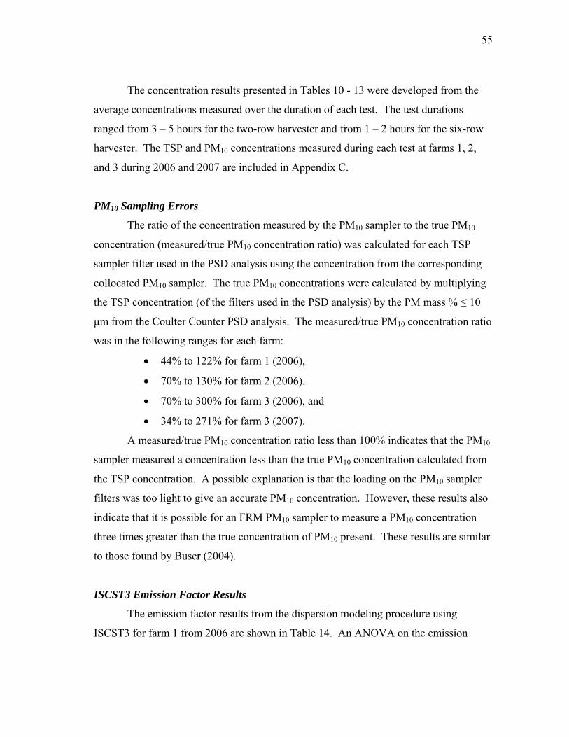
55
The concentration results presented in Tables 10 - 13 were developed from the
average concentrations measured over the duration of each test. The test durations
ranged from 3 – 5 hours for the two-row harvester and from 1 – 2 hours for the six-row
harvester. The TSP and PM10 concentrations measured during each test at farms 1, 2,
and 3 during 2006 and 2007 are included in Appendix C.
PM10 Sampling Errors
The ratio of the concentration measured by the PM10 sampler to the true PM10
concentration (measured/true PM10 concentration ratio) was calculated for each TSP
sampler filter used in the PSD analysis using the concentration from the corresponding
collocated PM10 sampler. The true PM10 concentrations were calculated by multiplying
the TSP concentration (of the filters used in the PSD analysis) by the PM mass % ≤ 10
μm from the Coulter Counter PSD analysis. The measured/true PM10 concentration ratio
was in the following ranges for each farm:
• 44% to 122% for farm 1 (2006),
• 70% to 130% for farm 2 (2006),
• 70% to 300% for farm 3 (2006), and
• 34% to 271% for farm 3 (2007).
A measured/true PM10 concentration ratio less than 100% indicates that the PM10
sampler measured a concentration less than the true PM10 concentration calculated from
the TSP concentration. A possible explanation is that the loading on the PM10 sampler
filters was too light to give an accurate PM10 concentration. However, these results also
indicate that it is possible for an FRM PM10 sampler to measure a PM10 concentration
three times greater than the true concentration of PM10 present. These results are similar
to those found by Buser (2004).
ISCST3 Emission Factor Results
The emission factor results from the dispersion modeling procedure using
ISCST3 for farm 1 from 2006 are shown in Table 14. An ANOVA on the emission

56
factor data by harvester treatment indicated no significant difference for any of the
harvester treatments (all p values > 0.3). The overall and treatment emission factor
means in terms of kg/ha and kg/bale are shown in Table 14. The mass %PM10 and PM2.5
used to convert the TSP emission factors to a PM10 and PM2.5 basis were 35.8 and 0.2%,
respectively. Detailed results of PSD analyses on the TSP samples are discussed later.
Table 14. Emission factor results from the dispersion modeling procedure using ISCST3 for farm 1 during 2006.
PM10 Emission
Factors PM2.5 Emission Factors TSP Emission
Factors Test Treatment (kg/ha) (kg/bale) (kg/ha) (kg/bale) (kg/ha) (kg/bale)
1 2 row 0.48 0.15 2.68E-03 8.56E-04 1.34 0.43 2 6 row 0.99 0.31 5.53E-03 1.71E-03 2.77 0.85 3 6 row w/ss+ 0.18 0.05 1.02E-03 2.67E-04 0.51 0.13 4 6 row 0.41 0.09 2.28E-03 5.10E-04 1.14 0.25 5 2 row 0.65 0.15 3.65E-03 8.38E-04 1.83 0.42 6 6 row 0.56 0.14 3.11E-03 7.61E-04 1.55 0.38 7 6 row w/ss 0.65 0.18 3.64E-03 1.03E-03 1.82 0.51 8 6 row 0.99 0.20 5.51E-03 1.10E-03 2.75 0.55 9 2 row 0.87 0.19 4.88E-03 1.07E-03 2.44 0.54
10 6 row w/ss 0.32 0.09 1.80E-03 4.82E-04 0.90 0.24 Overall Means 0.61 0.15 3.41E-03 8.62E-04 1.70 0.43
2 Row Means* 0.67a 0.17d 3.74E-03b 9.22E-04e 1.87c 0.46f 6 Row Means* 0.73a 0.18d 4.10E-03b 1.02E-03e 2.05c 0.51f
6 Row w/ss Means* 0.39a 0.11d 2.15E-03b 5.92E-04e 1.08c 0.30f +Emission factors reported for the 6 row w/ss treatment were developed from the methods described in protocol I using the upwind/downwind measured concentrations and not by the source sampling protocol. *Means with the same letter are not significantly different at the 0.05 level of significance by Fisher’s LSD test.
The emission factor results from ISCST3 in terms of kg/ha and kg/bale for farm
2 during 2006 are shown in Table 15. Similar to the data presented for farm 1, an
ANOVA on the farm 2 emission factor data indicated no significant differences by
harvesting treatment within any PM size range (i.e. PM10, PM2.5, TSP) for either
emission factor basis (all p values > 0.286). The mass %PM10 and PM2.5 used to convert
the TSP emission factors to a PM10 and PM2.5 basis were 48.8 and 0.2%, respectively.
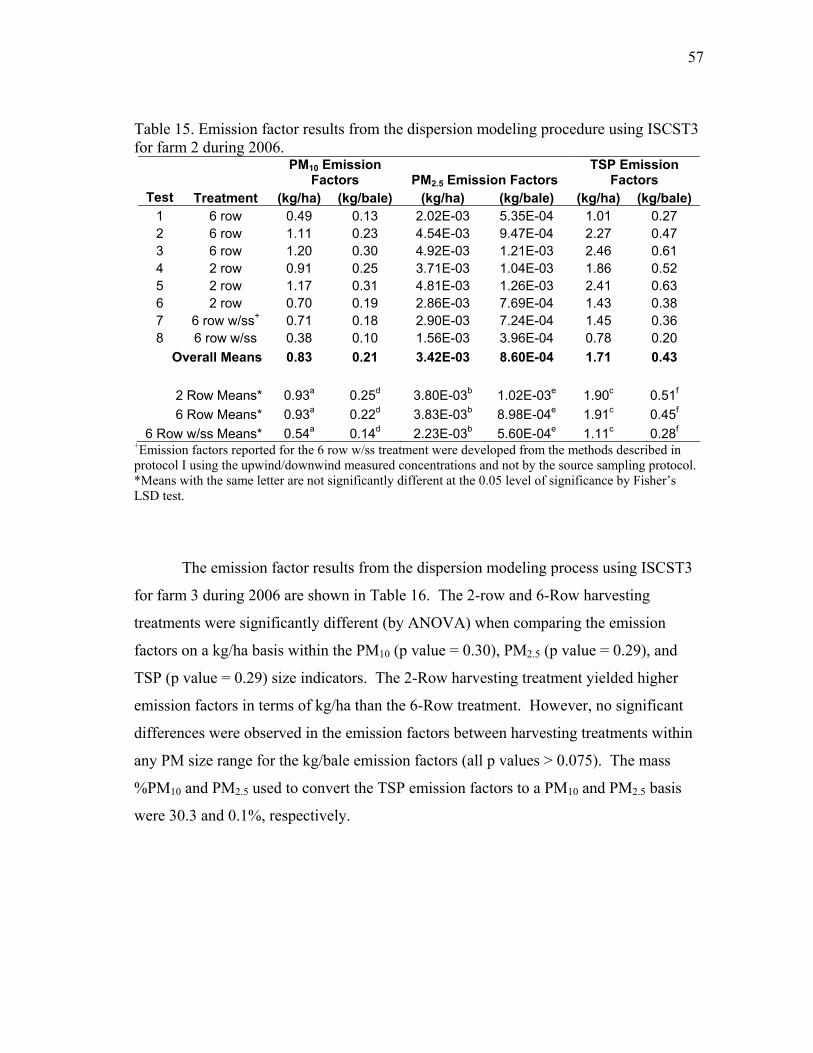
57
Table 15. Emission factor results from the dispersion modeling procedure using ISCST3 for farm 2 during 2006.
PM10 Emission
Factors PM2.5 Emission Factors TSP Emission
Factors Test Treatment (kg/ha) (kg/bale) (kg/ha) (kg/bale) (kg/ha) (kg/bale)
1 6 row 0.49 0.13 2.02E-03 5.35E-04 1.01 0.27 2 6 row 1.11 0.23 4.54E-03 9.47E-04 2.27 0.47 3 6 row 1.20 0.30 4.92E-03 1.21E-03 2.46 0.61 4 2 row 0.91 0.25 3.71E-03 1.04E-03 1.86 0.52 5 2 row 1.17 0.31 4.81E-03 1.26E-03 2.41 0.63 6 2 row 0.70 0.19 2.86E-03 7.69E-04 1.43 0.38 7 6 row w/ss+ 0.71 0.18 2.90E-03 7.24E-04 1.45 0.36 8 6 row w/ss 0.38 0.10 1.56E-03 3.96E-04 0.78 0.20
Overall Means 0.83 0.21 3.42E-03 8.60E-04 1.71 0.43
2 Row Means* 0.93a 0.25d 3.80E-03b 1.02E-03e 1.90c 0.51f 6 Row Means* 0.93a 0.22d 3.83E-03b 8.98E-04e 1.91c 0.45f
6 Row w/ss Means* 0.54a 0.14d 2.23E-03b 5.60E-04e 1.11c 0.28f +Emission factors reported for the 6 row w/ss treatment were developed from the methods described in protocol I using the upwind/downwind measured concentrations and not by the source sampling protocol. *Means with the same letter are not significantly different at the 0.05 level of significance by Fisher’s LSD test.
The emission factor results from the dispersion modeling process using ISCST3
for farm 3 during 2006 are shown in Table 16. The 2-row and 6-Row harvesting
treatments were significantly different (by ANOVA) when comparing the emission
factors on a kg/ha basis within the PM10 (p value = 0.30), PM2.5 (p value = 0.29), and
TSP (p value = 0.29) size indicators. The 2-Row harvesting treatment yielded higher
emission factors in terms of kg/ha than the 6-Row treatment. However, no significant
differences were observed in the emission factors between harvesting treatments within
any PM size range for the kg/bale emission factors (all p values > 0.075). The mass
%PM10 and PM2.5 used to convert the TSP emission factors to a PM10 and PM2.5 basis
were 30.3 and 0.1%, respectively.
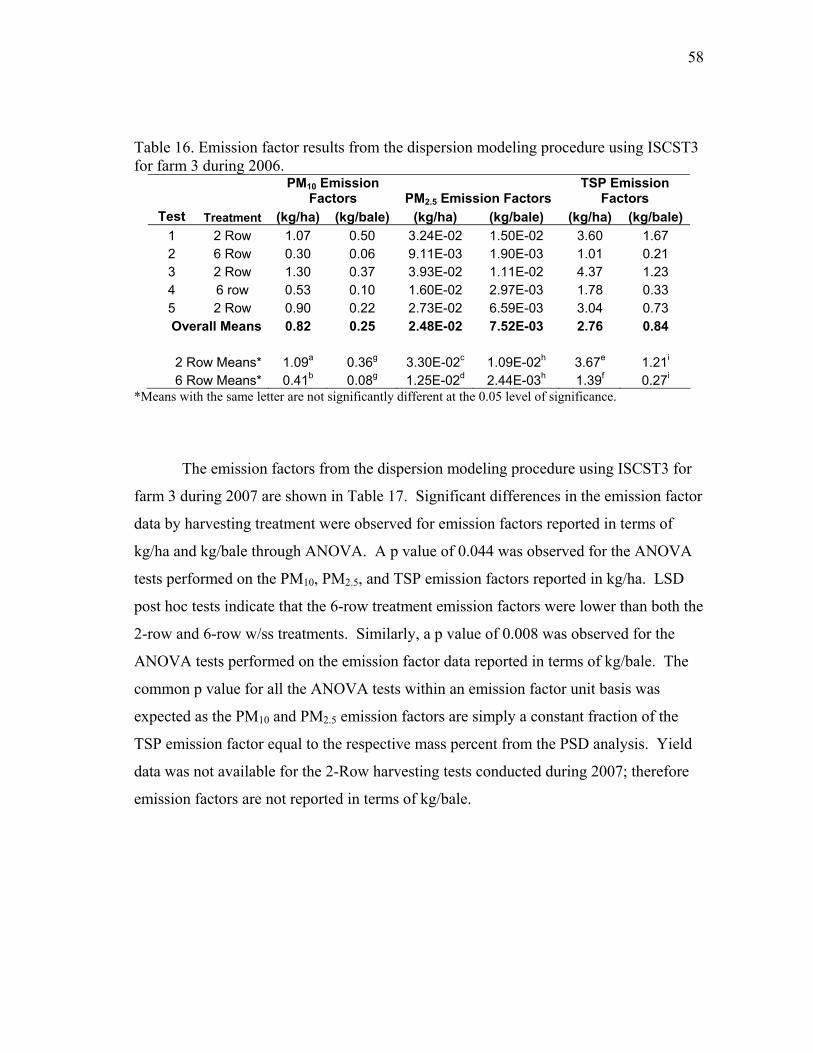
58
Table 16. Emission factor results from the dispersion modeling procedure using ISCST3 for farm 3 during 2006.
PM10 Emission
Factors PM2.5 Emission Factors TSP Emission
Factors Test Treatment (kg/ha) (kg/bale) (kg/ha) (kg/bale) (kg/ha) (kg/bale)
1 2 Row 1.07 0.50 3.24E-02 1.50E-02 3.60 1.67 2 6 Row 0.30 0.06 9.11E-03 1.90E-03 1.01 0.21 3 2 Row 1.30 0.37 3.93E-02 1.11E-02 4.37 1.23 4 6 row 0.53 0.10 1.60E-02 2.97E-03 1.78 0.33 5 2 Row 0.90 0.22 2.73E-02 6.59E-03 3.04 0.73 Overall Means 0.82 0.25 2.48E-02 7.52E-03 2.76 0.84 2 Row Means* 1.09a 0.36g 3.30E-02c 1.09E-02h 3.67e 1.21i 6 Row Means* 0.41b 0.08g 1.25E-02d 2.44E-03h 1.39f 0.27i
*Means with the same letter are not significantly different at the 0.05 level of significance.
The emission factors from the dispersion modeling procedure using ISCST3 for
farm 3 during 2007 are shown in Table 17. Significant differences in the emission factor
data by harvesting treatment were observed for emission factors reported in terms of
kg/ha and kg/bale through ANOVA. A p value of 0.044 was observed for the ANOVA
tests performed on the PM10, PM2.5, and TSP emission factors reported in kg/ha. LSD
post hoc tests indicate that the 6-row treatment emission factors were lower than both the
2-row and 6-row w/ss treatments. Similarly, a p value of 0.008 was observed for the
ANOVA tests performed on the emission factor data reported in terms of kg/bale. The
common p value for all the ANOVA tests within an emission factor unit basis was
expected as the PM10 and PM2.5 emission factors are simply a constant fraction of the
TSP emission factor equal to the respective mass percent from the PSD analysis. Yield
data was not available for the 2-Row harvesting tests conducted during 2007; therefore
emission factors are not reported in terms of kg/bale.
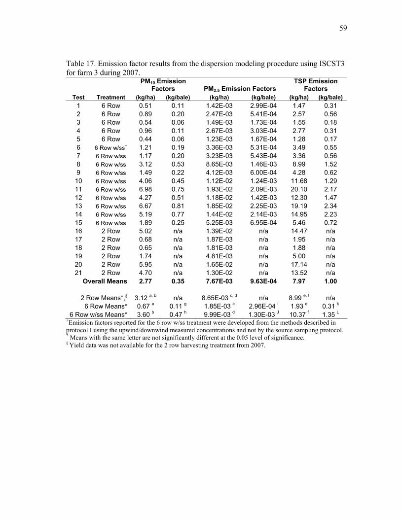
59
Table 17. Emission factor results from the dispersion modeling procedure using ISCST3 for farm 3 during 2007.
PM10 Emission
Factors PM2.5 Emission Factors TSP Emission
Factors Test Treatment (kg/ha) (kg/bale) (kg/ha) (kg/bale) (kg/ha) (kg/bale)
1 6 Row 0.51 0.11 1.42E-03 2.99E-04 1.47 0.31 2 6 Row 0.89 0.20 2.47E-03 5.41E-04 2.57 0.56 3 6 Row 0.54 0.06 1.49E-03 1.73E-04 1.55 0.18 4 6 Row 0.96 0.11 2.67E-03 3.03E-04 2.77 0.31 5 6 Row 0.44 0.06 1.23E-03 1.67E-04 1.28 0.17 6 6 Row w/ss+ 1.21 0.19 3.36E-03 5.31E-04 3.49 0.55 7 6 Row w/ss 1.17 0.20 3.23E-03 5.43E-04 3.36 0.56 8 6 Row w/ss 3.12 0.53 8.65E-03 1.46E-03 8.99 1.52 9 6 Row w/ss 1.49 0.22 4.12E-03 6.00E-04 4.28 0.62
10 6 Row w/ss 4.06 0.45 1.12E-02 1.24E-03 11.68 1.29 11 6 Row w/ss 6.98 0.75 1.93E-02 2.09E-03 20.10 2.17 12 6 Row w/ss 4.27 0.51 1.18E-02 1.42E-03 12.30 1.47 13 6 Row w/ss 6.67 0.81 1.85E-02 2.25E-03 19.19 2.34 14 6 Row w/ss 5.19 0.77 1.44E-02 2.14E-03 14.95 2.23 15 6 Row w/ss 1.89 0.25 5.25E-03 6.95E-04 5.46 0.72 16 2 Row 5.02 n/a 1.39E-02 n/a 14.47 n/a 17 2 Row 0.68 n/a 1.87E-03 n/a 1.95 n/a 18 2 Row 0.65 n/a 1.81E-03 n/a 1.88 n/a 19 2 Row 1.74 n/a 4.81E-03 n/a 5.00 n/a 20 2 Row 5.95 n/a 1.65E-02 n/a 17.14 n/a 21 2 Row 4.70 n/a 1.30E-02 n/a 13.52 n/a
Overall Means 2.77 0.35 7.67E-03 9.63E-04 7.97 1.00
2 Row Means*,§ 3.12 a, b n/a 8.65E-03 c, d n/a 8.99 e, f n/a 6 Row Means* 0.67 a 0.11 g 1.85E-03 c 2.96E-04 i 1.93 e 0.31 k
6 Row w/ss Means* 3.60 b 0.47 h 9.99E-03 d 1.30E-03 J 10.37 f 1.35 L +Emission factors reported for the 6 row w/ss treatment were developed from the methods described in protocol I using the upwind/downwind measured concentrations and not by the source sampling protocol. * Means with the same letter are not significantly different at the 0.05 level of significance. § Yield data was not available for the 2 row harvesting treatment from 2007.
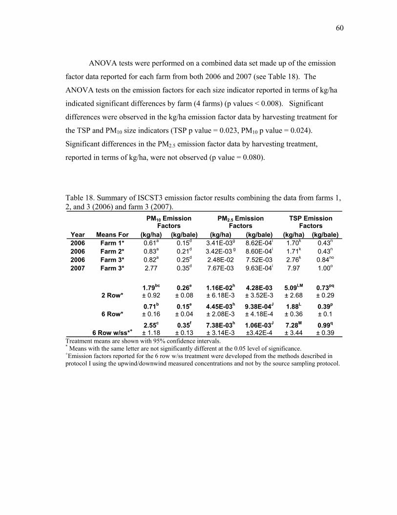
60
ANOVA tests were performed on a combined data set made up of the emission
factor data reported for each farm from both 2006 and 2007 (see Table 18). The
ANOVA tests on the emission factors for each size indicator reported in terms of kg/ha
indicated significant differences by farm (4 farms) (p values < 0.008). Significant
differences were observed in the kg/ha emission factor data by harvesting treatment for
the TSP and PM10 size indicators (TSP p value = 0.023, PM10 p value = 0.024).
Significant differences in the PM2.5 emission factor data by harvesting treatment,
reported in terms of kg/ha, were not observed (p value = 0.080).
Table 18. Summary of ISCST3 emission factor results combining the data from farms 1, 2, and 3 (2006) and farm 3 (2007).
PM10 Emission
Factors PM2.5 Emission
Factors TSP Emission
Factors Year Means For (kg/ha) (kg/bale) (kg/ha) (kg/bale) (kg/ha) (kg/bale) 2006 Farm 1* 0.61a 0.15d 3.41E-03g 8.62E-04i 1.70k 0.43n 2006 Farm 2* 0.83a 0.21d 3.42E-03 g 8.60E-04i 1.71k 0.43n 2006 Farm 3* 0.82a 0.25d 2.48E-02 7.52E-03 2.76k 0.84no 2007 Farm 3* 2.77 0.35d 7.67E-03 9.63E-04i 7.97 1.00o
2 Row* 1.79bc
± 0.92 0.26e
± 0.08 1.16E-02h ± 6.18E-3
4.28E-03 ± 3.52E-3
5.09LM ± 2.68
0.73pq ± 0.29
6 Row* 0.71b
± 0.16 0.15e
± 0.04 4.45E-03h
± 2.08E-3 9.38E-04J
± 4.18E-4 1.88L
± 0.36 0.39p
± 0.1
6 Row w/ss*+ 2.55c
± 1.18 0.35f
± 0.13 7.38E-03h
± 3.14E-3 1.06E-03J
±3.42E-4 7.28M
± 3.44 0.99q
± 0.39 Treatment means are shown with 95% confidence intervals. * Means with the same letter are not significantly different at the 0.05 level of significance. +Emission factors reported for the 6 row w/ss treatment were developed from the methods described in protocol I using the upwind/downwind measured concentrations and not by the source sampling protocol.
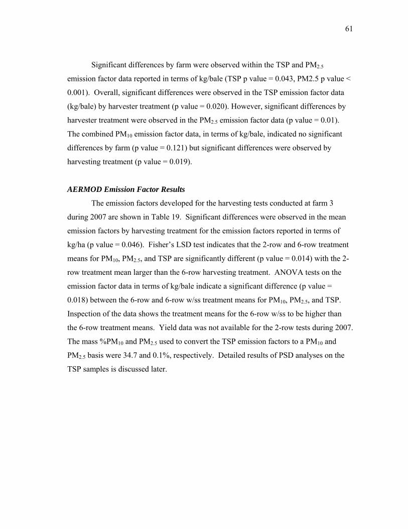
61
Significant differences by farm were observed within the TSP and PM2.5
emission factor data reported in terms of kg/bale (TSP p value = 0.043, PM2.5 p value <
0.001). Overall, significant differences were observed in the TSP emission factor data
(kg/bale) by harvester treatment (p value = 0.020). However, significant differences by
harvester treatment were observed in the PM2.5 emission factor data (p value = 0.01).
The combined PM10 emission factor data, in terms of kg/bale, indicated no significant
differences by farm (p value = 0.121) but significant differences were observed by
harvesting treatment (p value = 0.019).
AERMOD Emission Factor Results
The emission factors developed for the harvesting tests conducted at farm 3
during 2007 are shown in Table 19. Significant differences were observed in the mean
emission factors by harvesting treatment for the emission factors reported in terms of
kg/ha (p value = 0.046). Fisher’s LSD test indicates that the 2-row and 6-row treatment
means for PM10, PM2.5, and TSP are significantly different (p value = 0.014) with the 2-
row treatment mean larger than the 6-row harvesting treatment. ANOVA tests on the
emission factor data in terms of kg/bale indicate a significant difference (p value =
0.018) between the 6-row and 6-row w/ss treatment means for PM10, PM2.5, and TSP.
Inspection of the data shows the treatment means for the 6-row w/ss to be higher than
the 6-row treatment means. Yield data was not available for the 2-row tests during 2007.
The mass %PM10 and PM2.5 used to convert the TSP emission factors to a PM10 and
PM2.5 basis were 34.7 and 0.1%, respectively. Detailed results of PSD analyses on the
TSP samples is discussed later.

62
Table 19. Emission factor results from the dispersion modeling procedure using AERMOD for farm 3 during 2007.
PM10 Emission
Factors PM2.5 Emission Factors TSP Emission
Factors Test Treatment (kg/ha) (kg/bale) (kg/ha) (kg/bale) (kg/ha) (kg/bale)
1 6 Row 0.87 0.18 2.42E-03 5.10E-04 2.52 0.53 2 6 Row 1.32 0.29 3.67E-03 8.04E-01 3.81 0.84 3 6 Row 1.65 0.19 4.57E-03 5.31E-01 4.75 0.55 4 6 Row 1.39 0.16 3.85E-03 4.37E-01 4.00 0.45 5 6 Row 0.30 0.04 8.43E-04 1.14E-01 0.88 0.12 6 6 Row w/ss+ 1.69 0.27 4.67E-03 7.39E-01 4.86 0.77 7 6 Row w/ss 1.28 0.21 3.54E-03 5.95E-01 3.68 0.62 8 6 Row w/ss 2.93 0.49 8.11E-03 1.37E+00 8.43 1.42 9 6 Row w/ss 1.62 0.24 4.50E-03 6.55E-01 4.68 0.68 10 6 Row w/ss 3.93 0.43 1.09E-02 1.20E+00 11.31 1.25 11 6 Row w/ss 4.98 0.54 1.38E-02 1.49E+00 14.34 1.55 12 6 Row w/ss 2.77 0.33 7.68E-03 9.18E-01 7.98 0.95 13 6 Row w/ss 5.22 0.64 1.45E-02 1.76E+00 15.02 1.83 14 6 Row w/ss 3.83 0.57 1.06E-02 1.58E+00 11.03 1.65 15 6 Row w/ss 1.35 0.18 3.73E-03 4.95E-01 3.88 0.51 16 2 Row 5.64 n/a 1.56E-02 n/a 16.23 n/a 17 2 Row 1.16 n/a 3.22E-03 n/a 3.35 n/a 18 2 Row 0.81 n/a 2.25E-03 n/a 2.34 n/a 19 2 Row 9.22 n/a 2.55E-02 n/a 26.55 n/a 20 2 Row 8.50 n/a 2.35E-02 n/a 24.46 n/a 21 2 Row 2.97 n/a 8.22E-03 n/a 8.54 n/a Overall Means 3.02 0.32 8.37E-03 8.46E-01 8.70 0.92
2 Row Means*§ 4.72a
± 2.92 n/a 1.31E-02c
± 0.0081 n/a 13.58e
± 8.39 n/a
6 Row Means* 1.11b
± 0.47 0.17g
± 0.08 3.07E-03d
± 0.0013 4.78E-4i
± 2.17E-4 3.19f
± 1.33 0.50k
± 0.22
6 Row w/ss Means* 2.96ab
± 0.92 0.39h
± 0.10 8.20E-03cd
± 0.0026 1.08E-3J
± 2.84E-4 8.52ef
± 2.64 1.12L
± 0.29 +Emission factors reported for the 6 row w/ss treatment were developed from the methods described in protocol I using the upwind/downwind measured concentrations and not by the source sampling protocol. * Means with the same letter are not significantly different at the 0.05 level of significance. § Yield data was not available for the 2 row harvesting treatment from 2007. Treatment means are displayed with 95% confidence intervals.
Emission Factor Analysis Summary
The emission factor data presented previously exhibits wide variation due to
meandering wind direction, source-to-receptor configuration, and low net mass on the
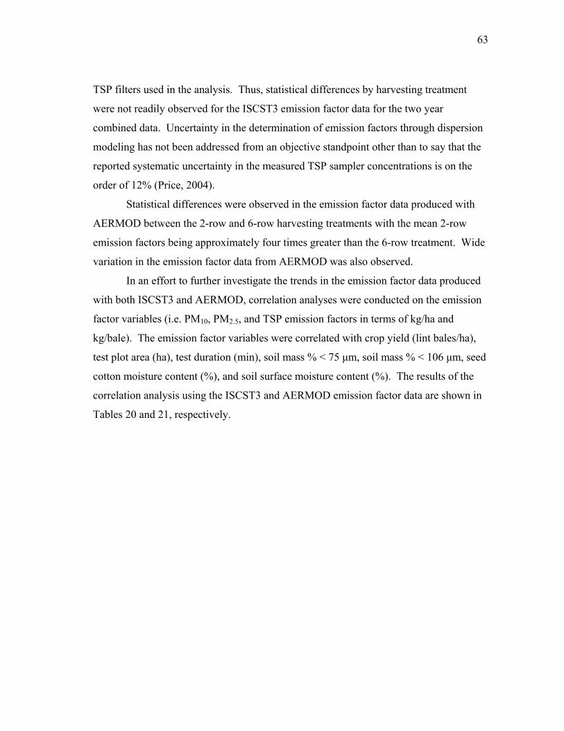
63
TSP filters used in the analysis. Thus, statistical differences by harvesting treatment
were not readily observed for the ISCST3 emission factor data for the two year
combined data. Uncertainty in the determination of emission factors through dispersion
modeling has not been addressed from an objective standpoint other than to say that the
reported systematic uncertainty in the measured TSP sampler concentrations is on the
order of 12% (Price, 2004).
Statistical differences were observed in the emission factor data produced with
AERMOD between the 2-row and 6-row harvesting treatments with the mean 2-row
emission factors being approximately four times greater than the 6-row treatment. Wide
variation in the emission factor data from AERMOD was also observed.
In an effort to further investigate the trends in the emission factor data produced
with both ISCST3 and AERMOD, correlation analyses were conducted on the emission
factor variables (i.e. PM10, PM2.5, and TSP emission factors in terms of kg/ha and
kg/bale). The emission factor variables were correlated with crop yield (lint bales/ha),
test plot area (ha), test duration (min), soil mass % < 75 μm, soil mass % < 106 μm, seed
cotton moisture content (%), and soil surface moisture content (%). The results of the
correlation analysis using the ISCST3 and AERMOD emission factor data are shown in
Tables 20 and 21, respectively.

64
Table 20. Correlation analysis results using the emission factor results produced with ISCST3. (significant correlations at the 0.01 level are highlighted)
ISCST3 Emission Factors TSP PM10 PM2.5 TSP PM10 PM2.5 (kg/ha) (kg/ha) (kg/ha) (kg/bale) (kg/bale) (kg/bale)
R 0.64 0.79 0.00 0.38 0.37 -0.29 Yield (bales/ha) p value <0.001 <0.001 0.995 0.019 0.022 0.080
R -0.60 -0.74 -0.07 -0.43 -0.46 0.17 Area (ha) p value <0.001 <0.001 0.653 0.008 0.003 0.318
R -0.32 -0.26 0.20 -0.13 -0.14 0.41 Test Duration (min) p value 0.033 0.089 0.194 0.437 0.395 0.011
R -0.10 0.13 0.08 -0.18 -0.26 0.24 Soil Mass % < 75 μm p value 0.522 0.410 0.598 0.284 0.123 0.158
R -0.12 0.14 0.06 -0.18 -0.26 0.24 Soil Mass % < 106 μm p value 0.456 0.384 0.698 0.294 0.133 0.167
R -0.05 0.03 -0.28 -0.07 -0.09 -0.28 Seed Cotton Moisture
Content (%) p value 0.743 0.860 0.068 0.665 0.597 0.092
R 0.04 0.18 0.04 -0.31 -0.32 -0.31 Soil Surface Moisture
Content (%) p value 0.878 0.440 0.878 0.278 0.271 0.278
The correlation results shown in Table 20 for the ISCST3 emission factors
indicate that the TSP and PM10 emission factors in terms of kg/ha are significantly
correlated with yield at the 0.01 level of significance. Similarly, the TSP and PM10
emission factors (for both kg/ha and kg/bale) are significantly correlated with the test
plot area at the 0.01 level of significance. The correlation values with regard to test plot
area are negative while those for yield are positive and slightly higher.
Significant correlations between yield and PM emission factors is logical in that
as the machines process more total material, so should PM emissions increase
proportionally. However, significant correlations with area seem not to follow intuition
as well. The observed negative correlations indicate that as the test plot area increases,
the emission factors on a mass/unit area and mass/bale basis decrease.
65
Table 21. Correlation analysis results using the emission factor results produced with AERMOD.
AERMOD Emission Factors TSP PM10 PM2.5 TSP PM10 PM2.5 (kg/ha) (kg/ha) (kg/ha) (kg/bale) (kg/bale) (kg/bale)
R 0.48 0.48 0.48 0.19 0.19 0.29 Yield (bales/ha)
p value 0.070 0.069 0.069 0.492 0.490 0.296
R -0.44 -0.44 -0.44 -0.29 -0.29 -0.42 Area (ha) p value 0.045 0.045 0.045 0.290 0.289 0.118
R 0.24 0.24 0.24 0.11 0.11 0.02 Test Duration (min)
p value 0.292 0.293 0.293 0.689 0.690 0.942
R 0.18 0.18 0.17 -0.45 -0.45 -0.39 Soil Mass % < 75 μm p value 0.446 0.447 0.449 0.096 0.095 0.148
R 0.24 0.24 0.24 -0.42 -0.42 -0.36 Soil Mass % < 106 μm p value 0.286 0.287 0.288 0.123 0.123 0.193
R -0.12 -0.12 -0.12 -0.06 -0.06 -0.10 Seed Cotton Moisture
Content (%) p value 0.609 0.608 0.608 0.828 0.828 0.736
R 0.20 0.20 0.19 -0.33 -0.33 -0.24 Soil Surface Moisture
Content (%) p value 0.409 0.408 0.410 0.242 0.243 0.406
The correlation analysis using the AERMOD emission factor data indicate no
significant correlations at the 0.01 level of significance. Although reduced in magnitude,
the correlation coefficients between the emission factor data and test plot area maintain
the previously observed indirect nature.
The correlation results between the emission factor data and the test plot area
may be an indication of fallacy in the steady state area source assumption in the
dispersion modeling process. In reality, the emissions generated by the cotton harvester
moving through the field is best described as a mobile point source.
The following general findings were observed from the emission factors
developed using Protocol I:

66
• As indicated by previous research, ISCST3 over estimates downwind concentrations
when used to predict hourly concentrations. Thus, sub-hourly variations in wind
direction and speed can be accounted for more appropriately in downwind
concentration predictions using meteorological data averaged over shorter time
periods on the order of 15 to 20 minutes.
• The amount of meteorological input data required by AERMOD is substantially
greater than the data required by ISCST3. Thus, the meteorological data processing
time is significantly increased for AERMOD.
• The majority of the additional meteorological input parameters required by
AERMOD (surface friction velocity, surface sensible heat flux, Monin-Obukhov
length, and convective velocity scale) can be calculated from wind vector and
temperature measurements taken by a 3D sonic anemometer. The remaining
parameters (temperature scale and potential temperature gradient) can be obtained
from radiosonde data of the upper atmosphere or through the empirical relationships
described by EPA (2004).
• AERMOD, the dispersion model recommended by EPA for regulatory purposes after
2007, characterizes dispersion within the planetary boundary layer under stable and
convective conditions by a mass weighted average, two plume state model. The first
plume state accounts for pollutants contained in the horizontal flow near the surface
of the Earth which do not possess sufficient kinetic energy to pass over or around
complex terrain features. The second plume state accounts for the mass of pollutants
in the turbulent flow region above the horizontal plume (state one) which have
sufficient kinetic energy to maintain entrainment when flowing around or over
complex terrain features.
• The emission factors calculated through the dispersion modeling process are greatly
dependent upon the source to receptor configuration. Variation in wind direction and
speed can exacerbate the variation incorporated in emission flux values determined
through the dispersion modeling process. An objective validation process was used
to identify receptor locations which would likely yield unreliable emission flux

67
estimates due to improper sampler operation, significant influence from outside
sources of PM, and the inability for the dispersion model to closely approximate the
dispersion of PM emissions from the source as observed through the concentrations
measured downwind.
• Errors were observed in the FRM PM10 sampler concentrations measured downwind
of the harvesting operations. The ratio of the true PM10 concentration to the
measured PM10 concentration varied by farm but ranged from 34 to 300%. True
PM10 concentrations were determined by multiplying the measured collocated TSP
concentration by the mass fraction of PM10 from PSD analysis.
• The treatment mean TSP emission factors in terms of kg/ha (lb/ac) from the 2006
and 2007 combined data set resulting from the dispersion modeling procedure using
ISCST3 are:
o 2-Row: 5.09 ± 2.68 kg/ha (4.54 ± 2.39 lb/ac),
o 6-Row: 1.88 ± 0.36 kg/ha (1.68 ± 0.32 lb/ac), and
o 6-Row w/SS: 7.28 ± 3.44 kg/ha (6.49 ± 3.07 lb/ac).
Emission factors reported for the 6 row w/ss treatment were developed from the
methods described in protocol I using the upwind/downwind measured
concentrations and not by the source sampling protocol.
• The treatment mean PM10 emission factors in terms of kg/ha (lb/ac) from the 2006
and 2007 combined data set resulting from the dispersion modeling procedure using
ISCST3 are:
o 2-Row: 1.79 ± 0.92 kg/ha (1.6 ± 0.82 lb/ac),
o 6-Row: 0.71 ± 0.16 kg/ha (0.63 ± 0.14 lb/ac), and
o 6-Row w/SS: 2.55 ± 1.18 kg/ha (2.27 ± 1.05 lb/ac).
• The treatment mean PM2.5 emission factors in terms of kg/ha (lb/ac) from the 2006
and 2007 combined data set resulting from the dispersion modeling procedure using
ISCST3 are:
o 2-Row: 1.16E-2 ± 6.18E-3 kg/ha (1.03E-2 ± 5.51E-3 lb/ac),
o 6-Row: 4.45E-3 ± 2.08E-3 kg/ha (3.97E-3 ± 1.86E-3 lb/ac), and
68
o 6-Row w/SS: 7.38E-3 ± 3.14E-3 kg/ha (6.58E-3 ± 2.8E-3 lb/ac).
• The treatment mean TSP emission factors in terms of kg/bale (lb/bale) from the 2006
and 2007 combined data set resulting from the dispersion modeling procedure using
ISCST3 are:
o 2-Row: 0.73 ± 0.29 kg/bale (1.61 ± .64 lb/bale),
o 6-Row: 0.39 ± 0.1 kg/bale (0.86 ± 0.22 lb/bale), and
o 6-Row w/SS: 0.99 ± 0.39 kg/bale (2.18 ± 0.86 lb/bale).
• The treatment mean PM10 emission factors in terms of kg/bale (lb/bale) from the
2006 and 2007 combined data set resulting from the dispersion modeling procedure
using ISCST3 are:
o 2-Row: 0.26 ± 0.08 kg/bale (0.57 ± 0.18 lb/bale),
o 6-Row: 0.15 ± 0.04 kg/bale (0.33 ± 0.09 lb/bale), and
o 6-Row w/SS: 0.35 ± 0.13 kg/bale (0.77 ± 0.29 lb/bale).
• The treatment mean PM2.5 emission factors in terms of kg/bale (lb/bale) from the
2006 and 2007 combined data set resulting from the dispersion modeling procedure
using ISCST3 are:
o 2-Row: 4.28E-3 ± 3.52E-3 kg/bale (9.43E-3 ±7.75E-3 lb/bale),
o 6-Row: 9.38E-4 ± 4.18E-4 kg/bale (2.07E-3 ± 9.21E-4 lb/bale), and
o 6-Row w/SS: 1.06E-3 ± 3.42E-4 kg/bale (2.34E-3 ± 7.53E-4 lb/bale).
• The combined ISCST3 emission factor data from 2006 and 2007 indicates that there
is not a significant difference in PM emission factors for any size indicator for the
two-row and six-row harvesting treatments (kg/ha emission factor basis). Similarly,
significant differences were not observed between the two-row and six-row
machines for the kg/bale data with the exception of the PM2.5 data. Although
significant differences were not observed, there is a substantial difference in the
mean emission factors for the two-row and six-row harvesting treatments. This
result is likely due to the great amount of variability introduced in the emission
factors from wind direction/speed variation.

69
• The TSP emission factors for farm 3 during 2007 in terms of kg/ha (lb/ac) from the
dispersion modeling process using AERMOD are:
o 2-Row: 13.58 ± 8.39 kg/ha (12.1 ± 7.48 lb/ac),
o 6-Row: 3.19 ± 1.33 kg/ha (2.84 ± 1.19 lb/ac), and
o 6-Row w/SS: 8.52 ± 2.64 kg/ha (7.59 ± 2.35 lb/ac).
• The PM10 emission factors for farm 3 during 2007 in terms of kg/ha (lb/ac) from the
dispersion modeling process using AERMOD are:
o 2-Row: 4.72 ± 2.92 kg/ha (4.21 ± 2.6 lb/ac),
o 6-Row: 1.11 ± 0.47 kg/ha (0.99 ± 0.42 lb/ac), and
o 6-Row w/SS: 2.96 ± 0.92 kg/ha (2.64 ± 0.82 lb/ac).
• The PM2.5 emission factors for farm 3 during 2007 in terms of kg/ha (lb/ac) from the
dispersion modeling process using AERMOD are:
o 2-Row: 1.31E-2 ± 0.008 kg/ha (0.012 ± 0.007 lb/ac),
o 6-Row: 3.07E-3 ± 0.0013 kg/ha (0.003 ± 0.0012 lb/ac), and
o 6-Row w/SS: 8.2E-3 ± 0.0026 kg/ha (0.073 ± 0.0023 lb/ac).
• The mean TSP emission factors in terms of kg/bale (lb/bale) from farm 3 during
2007 resulting from the dispersion modeling procedure using AERMOD are (yield
data was not available for the 2-Row treatment):
o 6-Row: 0.50 ± 0.22 kg/bale (1.1 ± 0.48 lb/bale), and
o 6-Row w/SS: 1.12 ± 0.29 kg/bale (2.47 ± 0.64 lb/bale).
• The mean PM10 emission factors in terms of kg/bale (lb/bale) from farm 3 during
2007 resulting from the dispersion modeling procedure using AERMOD are:
o 6-Row: 0.17 ± 0.08 kg/bale (0.37 ± 0.18 lb/bale), and
o 6-Row w/SS: 0.39 ± 0.1 kg/bale (0.86 ± 0.22 lb/bale).
• The mean PM2.5 emission factors in terms of kg/bale (lb/bale) from farm 3 during
2007 resulting from the dispersion modeling procedure using AERMOD are:
o 6-Row: 4.78E-4 ± 2.17E-4 kg/bale (0.001 ± 0.0005 lb/bale), and
o 6-Row w/SS: 1.08E-3 ± 2.84E-4 kg/bale (0.002 ± 0.0006 lb/bale).

70
• Significant differences were observed in the mean emission factors developed with
AERMOD for the two-row and six-row treatments, for all size indicators. The 2-row
and 6-row emission factors generated with AERMOD were larger than the emission
factors generated with ISCST3for the tests performed on farm 3 during 2007.
However, the 6-row w/SS emission factors generated in ISCST3 were higher than
those generated in AERMOD for the farm 3, 2007 data.
• The emission factor data developed in ISCST3 were found to be significantly
correlated with crop yield and test plot area. However, significant correlations were
not observed between the emission factor data developed in AERMOD and crop
yield or test plot area. These results may be indicative of problems in the assumption
that the dispersion from the harvesting operation can be closely approximated by an
area source model with a constant emission flux.

71
CHAPTER IV
EMISSION FACTOR DEVELOPMENT PROTOCOL II:
SOURCE MEASUREMENT OF EMISSION CONCENTRATIONS
INTRODUCTION
Little accurate emission factor data exists for agricultural field operations. The
data that does exist has been developed through indirect measurement techniques similar
to those described in the previous section. The indirect measurement technique used in
this work for emission factor development relies on mathematical models with
unspecified levels of uncertainty which may vary with meteorological conditions such as
wind direction and wind speed, among others. Further, the variation introduced into the
predicted emission factors due to the estimation of meteorological parameters through
theoretical and empirical relationships is undefined. Nonetheless, dispersion models
play a key role in the air pollution regulatory process to protect human health through
the estimation of downwind concentrations resulting from source emissions.
Agricultural and industrial sources of PM should be permitted based on accurate
emission factors. Ideally, these emission factors would be obtainable through both
indirect and direct measurements. A premise of the emission factor development
protocol discussed in this section is that the conservative nature of regulatory dispersion
models tends to produce emission factor estimates that do not accurately reflect true
source emission levels. Although an emission factor developed through this process will
result in the close approximation of downwind concentrations from an agricultural
source, the emission factor may lead to the inappropriate regulation of an agricultural
source when regulations are based on emission inventory levels. It is also a premise of
this method that accurate emission factors can be developed through direct source
measurement of PM emission rates.
72
PROTOTYPE DEVELOPMENT AND FIRST YEAR TESTING
A prototype source sampling system (Figure 9, 10, and 11) was designed and
used onboard a John Deere model 9996 cotton picker during the first year of the study.
The source sampling system was designed to collect all of the air, seed cotton, and
foreign material (plant material, soil, etc.) from one of the ducts on the six-row
harvester, separate the seed cotton from the air stream, and exhaust the particulate laden
air stream after performing an isokinetic emission concentration measurement.
Pitot tube traverses were performed on the six ducts which transport the seed
cotton from the picking units to the basket to determine the average air velocity in each
duct. The average air velocities ranged from 1070 to 1525 m/min (3500 – 5000 ft/min)
across the six ducts. The maximum average velocity was observed in duct 3 (numbering
the ducts from left to right sitting in the operator seat). Thus, the source sampling
system was designed for use on duct 3 so that any increase in static pressure loss caused
by the source sampler would lower the average duct velocity (in duct 3) to a value closer
to that observed for the other ducts. The average air velocity measured at the exit of the
source sampler was approximately 914 m min-1 (3000 ft min-1) after the source sampler
was installed on duct 3. The air flow rate of each duct was calculated by multiplying the
average velocities determined by the pitot tube traverse by the cross sectional area of
each duct (duct area = 0.093 m2 = 1 ft2).
Separation of the seed cotton from the air stream was accomplished in the
separator section by means of a baffle type separator (see Figures 9, 10, and 11). The
inlet duct to the separator section maintained the cross sectional area (20.3 x 45.7 cm) of
the harvester duct so that the velocity of the seed cotton and air would be approximately
the same entering the baffle type separator as it was exiting duct 3. The critical air
velocity, as described by Mihalski (1996), used for the design of the baffle separation
section was 305 m/min (1000 ft/min). The critical air velocity was provided by
increasing the flow area at the edge of the baffle to four times that of the inlet area. It is
expected that the actual air velocity at the edge of the baffle was less than the designed
critical velocity due to a decrease of the inlet air velocity caused by static pressure loss
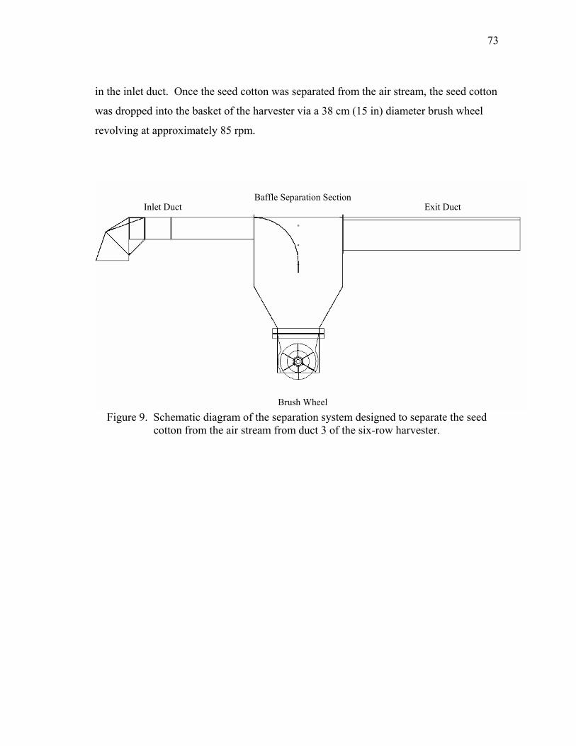
73
in the inlet duct. Once the seed cotton was separated from the air stream, the seed cotton
was dropped into the basket of the harvester via a 38 cm (15 in) diameter brush wheel
revolving at approximately 85 rpm.
Figure 9. Schematic diagram of the separation system designed to separate the seed
cotton from the air stream from duct 3 of the six-row harvester.
Brush Wheel
Baffle Separation Section Inlet Duct Exit Duct

74
Figure 10. Detail drawing of separator box design 1 showing interior curved baffle (side
view). All dimensions are in cm.

75
Figure 11. Schematic drawing of separator box design 1 with general dimensions shown (isometric view). All dimensions are in cm.
The particulate laden air was exhausted through a 1.6 m (64 in) exit duct. The
cross section dimensions of the exit duct were 30.5 cm x 30.5 cm (1 ft x 1 ft). The
velocity pressure of the air in the exit duct was measured by a pitot tube located in the
center of the duct approximately 40.6 cm (16 in) from the exit and the air velocity was
calculated according to equation 41.
a
vPV
ρ01.14= (41)
where V = air velocity (m/s), Pv = velocity pressure measured by pitot tube (cm H2O),
and ρa = air density (kg/m3).
An isokinetic emission concentration measurement was taken at the center of the
duct approximately 20.3 cm (8 in) from the exit. The PM laden air captured by the
isokinetic sampler nozzle was passed though a 15.2 cm (6 in) diameter barrel type
Exit
Inlet

76
cyclone (Tullis et.al., 1997) to separate the large PM from the air stream. The PM which
penetrated the cyclone was captured on a bank of four, 20.3 by 25.4 cm coated
borosilicate glass microfiber filters (Pall Corp., Pallflex Emfab filter material 7224, East
Hills, NY).
The designed maximum air flow rate of the isokinetic sampler was 2.12 m3 min-1
(75 ft3 min-1) and was measured by an orifice meter. The orifice diameter of 53.64 mm
(2.112 in) was specified such that the pressure drop across the orifice plate would be
equal to the velocity pressure of the duct (measured by the pitot tube) when the velocity
of the air entering the sampler nozzle was equal to the velocity of the air in the exit duct
(thus producing an isokinetic sample of the air exiting the harvester). This was done to
simplify the operation of the sampler control system. The system operator (sitting inside
the cab of the harvester) maintained the isokinetic sampling condition by controlling the
speed of the fans using a variable transformer (Dayton E165942, Dayton Electric
Manufacturing Co., Niles, IL). The sampler air flow was provided by two fans (Model
HP-33, Clements National Company, Chicago, IL) installed in series mounted on top of
the harvester and the diameter of the sampling nozzle was 47 mm (1.85 in). Pressure
transducers (PX274, Omega Engineering, Inc., Stamford, Conn.) were used to measure
the velocity pressure from the pitot tube in the exit duct, the pressure drop across the
orifice plate, and the pressure drop across the filter housings (to give a measure of the
filter loading). Data loggers (HOBO H8 RH/Temp/2x External, Onset Computer Corp,
Pocasset, Mass) were used to record the differential pressure readings from the pressure
transducers over the duration of the test.
The emission concentration measured by the source sampler was calculated
according to equation 42.
∑
+=
iii
BF
tQMMEC (42)
where EC = emission concentration (g/m3), MF = PM mass on the four filters used in the
source sampler (g), MB = PM mass < 100μm captured in the cyclone bucket (g), Qi = air
flow rate during the ith logging interval (m3/s1), and ti = ith logging interval (6 sec).

77
The cyclone bucket contained all of the material separated from the sampled air
stream by the cyclone. This material was primarily plant and soil material with small
amounts of lint fiber and PM. The material taken from the cyclone bucket was air
washed for 15 minutes (1.1 m3 min-1 air flow rate, 60 rpm tumbler rotation speed) to
remove the PM <100 μm (Wanjura et al., 2007). The air wash tumbler was covered with
100 μm stainless steel mesh and the extracted PM was collected on a 20.3 by 25.4 cm
borosilicate glass microfiber filter (Pall Corp., Pallflex Emfab filter material, East Hills,
NY). All of the filters used in the source sampler and in the air washing process of the
cyclone bucket material were pre and post weighed according to the procedure described
by Wanjura et al. (2005b).
The total mass of PM emitted from duct 3 during the test was calculated by
multiplying the emission concentration (equation 42) by the total volume of air passing
through the duct. The total mass of PM emitted from the harvester was estimated by
multiplying the total PM mass emission from duct 3 by 6 (the number of picking
units/seed cotton transport ducts on the harvester). It was assumed that the total mass of
PM emitted from one duct was constant across all of the ducts. TSP emission factors
were calculated by dividing the total mass of PM emitted by the harvester by either the
area harvested or the number of 218 kg (480 lb) bales harvested to obtain emission
factors in units of mass of TSP per area harvested or per bale harvested, respectively.
The total mass of lint harvested (bales) was estimated by multiplying the weight of seed
cotton harvested during each test by an estimated 34% lint turnout and dividing by 218
kg/bale (480 lb/bale). Seed cotton weights were obtained from a boll buggy equipped
with load cells. PM10 and PM2.5 emission factors were obtained by multiplying the TSP
emission factors by the respective mass fractions from the results of PSD analyses on the
filters.
Wanjura et al. (2007) reported overall average TSP, PM10, and PM2.5 source
sampler emission factors of 114, 45, and 0.15 g/ha, respectively. They also reported
overall average TSP, PM10, and PM2.5 source sampler emission factors of 10, 4, and 0.01
g/bale, respectively. The authors stated that the emission factors developed by the
78
source sampling system exhibited much higher precision than the comparable emission
factors developed using a protocol employing ground level samplers downwind of the
harvesting operation. However, the reported emission factors developed by the source
sampling system were developed from four tests conducted at two locations during the
2006 south Texas cotton harvest season.
SEED COTTON SEPARATION SYSTEM DESIGN MODIFICATION AND
EVALUATION
Separator Box Design and Evaluation
The system designed to separate seed cotton from the air stream on the six-row
picker was mounted on a test frame to facilitate testing and evaluation (Figure 12). Two
centrifugal fans (PB-18, Cincinnati Fan, Mason, OH) connected in parallel provided the
air flow to transport seed cotton from the feeder through the system. The fans were
operated on a hydraulic circuit powered by a 37.3 kW (50 hp) pressure compensated
pump (Eaton PVB45, Eaton Hydraulics, Eden Prairie, MN). Fan speed was controlled
through a flow control valve which regulated the high pressure fluid flow to the
hydraulic motor (Parker PGM315, Parker Hannifin, Youngstown, OH). The hydraulic
motor was connected to the fan rotors via a belt drive with a speed increasing ratio of
2:1. The total air flow through the system was maintained at 85 ± 0.85 m3 min-1 (3000 ±
30 ft3 min-1). The air flow rate from each fan was determined using equation 43 and
center point velocity pressure measurements taken in the 12.7 cm (5 in) diameter ducts
located between the discharge of each fan and the inlet to the seed cotton feeder.
a
CPVi
FPdQ
ρπ
)(15.210 ,2= (43)
where Qi = air flow rate from fan i (m3/min), d = duct diameter (m), PV,CP = center point
velocity pressure (cm H2O), F = center point correction factor, and ρa = air density
(kg/m3).

79
Figure 12. Photo of seed cotton separation system mounted in the testing frame
configured with the seed cotton feeder and fan system.
Velocity pressure measurements were taken at 20 locations along 2 perpendicular
diameters of the fan ducts to determine the average velocity pressure in each duct. The
center point correction factor (F) was calculated for each duct as the ratio of the duct
average velocity pressure to the center point velocity pressure. Thus, the center point
velocity pressure measurements taken prior to each test were corrected to the duct
average velocity pressure using the center point correction factor in order to determine
the flow rate from each fan. All velocity pressure measurements were taken using a
pitot tube (Model 166-12, W.E. Anderson, Michigan City, IN) and digital magnehelic
gage (475-1-FM, Dwyer Instruments, Inc., Michigan City, IN).
Seed Cotton Separation System
Seed Cotton Feeding System
Fans
80
Air dry bulb temperature, relative humidity, and barometric pressure were
measured during each test using a weather station (Temp/RH Sensor: Model S-THB-
M002; Barometric Pressure Sensor: Model S-BPA-CM10, Onset Computer Corporation,
Pocasset, MA). These measurements were used to calculate the density of the air as
shown in equation 4.
The feeder used to introduce seed cotton into the air stream (figure 13) consisted
of a set of upper paddle rollers rotating inward in opposite directions to pull the seed
cotton from the hopper onto a set of spiked rollers rotating at approximately twice the
speed of the upper rollers. The lower spiked rollers helped to open clumped masses of
seed cotton pressed together by the paddle rollers and provide more uniform feeding of
the seed cotton into the air stream. The seed cotton feeder was operated by a hydraulic
motor (Char-Lynn H Series 101-1008, Eaton Hydraulics, Eden Prairie, MN) powered by
a 22.4 kW (30 hp) pressure compensated pump (Eaton PVB29, Eaton Hydraulics, Eden
Prairie, MN). The feed rate of seed cotton into the system was controlled by regulating
the speed of the upper rollers of the feeder. Thus a flow control valve was used to
control the speed of the hydraulic motor. During each test, 18.2 kg (40 lb) lots of seed
cotton were fed through the system at nominal feed rates of 22.7, 45.4, and 68.1 kg/min
(50, 100, and 150 lbs/min). These feed rates are approximately equivalent to the
harvesting rate of a single row unit gathering seed cotton in yields of 1, 2, and 3 bales
per acre, respectively (assuming: 101.6 cm row spacing, 681 kg of seed cotton per bale,
and 6.4 km h-1 picking speed).
Two separator box designs were evaluated with several different baffle
configurations to determine the separator box/baffle configuration which resulted in the
lowest mass of seed cotton penetrating the exit duct. The first separator box design was
tested with three curved baffle configurations with overall lengths of 30.5, 40.6, and 47
cm (12, 16, and 18.5 in). Each baffle was positioned so that the lower edge of the baffle
was 40.6 cm (16 in) from the front wall of the separator box. Clear polycarbonate
material was placed on one side wall of both separator box designs so that visual
observations of the cotton flowing through the system could be made. During testing of

81
separator box design 1 it was observed that seed cotton accumulated on the inclined back
wall of the box before falling into the brush wheel. It was further observed that the seed
cotton which accumulated in this area was easily re-entrained in the air stream allowing
it to penetrate to the exit duct. Therefore, the design of separator box 2 (Figures 13, 14,
and 15) included a straight back wall so to minimize the accumulation of seed cotton
before the brush wheel. This design modification resulted in the movement of the brush
wheel to the back wall of the separator box where as it was located at the center of
separator box design 1.
Figure 13. Schematic drawing of separator box design 2 illustrating the straight back
wall design with the brush wheel moved to the rear of the separator box.
Straight Back Wall
Brush Wheel
Baffle Separation Section Inlet Duct Exit Duct
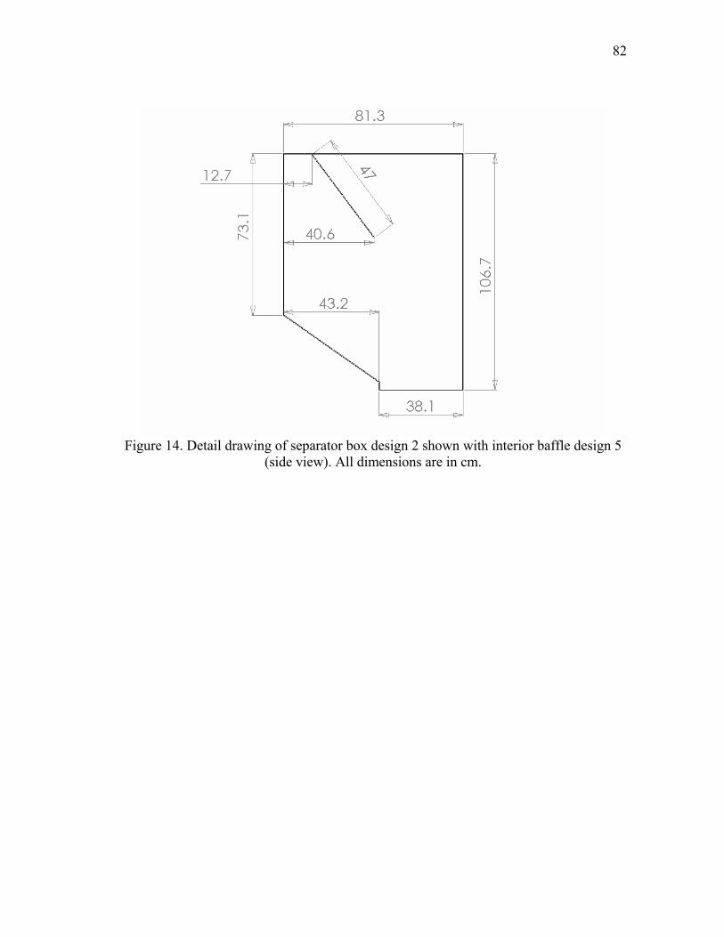
82
Figure 14. Detail drawing of separator box design 2 shown with interior baffle design 5
(side view). All dimensions are in cm.
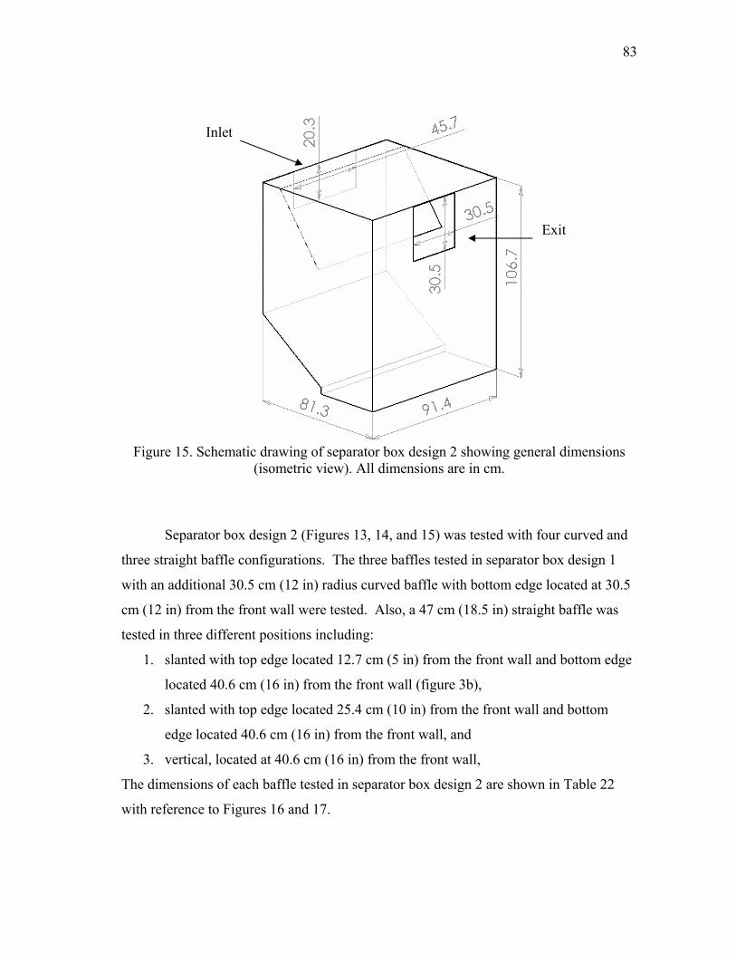
83
Figure 15. Schematic drawing of separator box design 2 showing general dimensions
(isometric view). All dimensions are in cm.
Separator box design 2 (Figures 13, 14, and 15) was tested with four curved and
three straight baffle configurations. The three baffles tested in separator box design 1
with an additional 30.5 cm (12 in) radius curved baffle with bottom edge located at 30.5
cm (12 in) from the front wall were tested. Also, a 47 cm (18.5 in) straight baffle was
tested in three different positions including:
1. slanted with top edge located 12.7 cm (5 in) from the front wall and bottom edge
located 40.6 cm (16 in) from the front wall (figure 3b),
2. slanted with top edge located 25.4 cm (10 in) from the front wall and bottom
edge located 40.6 cm (16 in) from the front wall, and
3. vertical, located at 40.6 cm (16 in) from the front wall,
The dimensions of each baffle tested in separator box design 2 are shown in Table 22
with reference to Figures 16 and 17.
Exit
Inlet

84
Each separator box/baffle configuration was tested at three nominal seed cotton
feed rates of 22.7, 45.4, and 68.1 kg/min (50, 100, and 150 lbs/min) with three
replications per feed rate. Actual feed rates were calculated for each test by dividing the
lot mass of seed cotton by the duration of the test. Each configuration was evaluated
based on the mass of seed cotton that penetrated the exit duct of the separator system.
The seed cotton penetrating the system was collected in a wire mesh bin attached to the
discharge end of the exit duct. The collection bin was weighed before and after each test
using a laboratory balance (Mettler-Toledo PM30, Mettler-Toledo, Inc., Columbus, OH).
Analysis of variance (ANOVA) and Tukey’s HSD tests were performed using the
general linear model in SPSS to determine differences in the separator box design/baffle
configurations.
Table 22. Description of the baffles tested in separator box designs 1 and 2. (see Figures 16 and 17)
R D X T L
Baffle No.
Tested in Separator
Box Design Numbers Shape cm (in) cm (in) cm (in) cm (in) cm (in)
1 1 and 2 Curved 30.5 (12) 40.6 (16) 0 - - 2 1 and 2 Curved 40.6 (16) 40.6 (16) 0 - - 3 1 and 2 Curved 40.6 (16) 40.6 (16) 6.4 (2.5) - - 4 2 only Curved 30.5 (12) 30.5 (12) 0 - - 5 2 only Straight - 40.6 (16) - 12.7 (5) 47 (18.5) 6 2 only Straight - 40.6 (16) - 25.4 (10) 47 (18.5) 7 2 only Straight - 40.6 (16) - 40.6 (16) 47 (18.5)

85
Figure 16. Schematic showing curved baffle dimensions for baffles 1, 2, 3, and 4 (see
Table 22.
Figure 17. Schematic showing straight baffle dimensions for baffles 5, 6, and 7 (see
Table 22).
T Inlet Duct
Exit Duct
D
L
R
D
Inlet Duct Exit Duct
X

86
Velocity Profile Testing
Air velocity measurements were taken at nine points across the cross section of
the exit duct to determine if consistent air flow patterns exist in the exit duct. The logic
was used that if consistent air flow patterns were present in the exit duct, it is likely that
a concentration profile also exists in the exit duct. Thus the air velocity profile was
investigated by dividing the cross section of the exit duct into nine equal area sections
and locating air velocity probes (641RM-12, Dwyer Instruments, Inc., Michigan City,
IN) at the centroid of each equal area region (see Figure 18). The velocity probes were
installed coplanar to one another at 20.3 cm (8 in) from the end of the exit duct. Air
velocity profile testing was only performed on separator box design 2 with the top and
bottom edges of the straight baffle located at 12.7 and 40.6 cm (5 and 16 in),
respectively (baffle 5, see Table 22).
The air velocity profile was measured at seed cotton feed rates of 0, 22.7, and
45.4 kg/min (0, 50, and 100 lb/min). Five replications at each seed cotton feed rate were
performed. During each test the system air flow rate (measured using a pitot tube in the
ducts on the exit side of the fans) was maintained at 85 m3/min (3000 ft3/min). Air
velocity readings at the nine locations in the exit duct were taken simultaneously using a
data acquisition system (cFP-AI-110, National Instruments, Austin, TX) controlled by a
laptop computer. The data acquisition system measured and recorded air velocity
readings on a 1 Hz frequency. Air temperature, relative humidity, and barometric
pressure were measured inside the exit duct using a temperature/RH sensor (HX94A,
Omega Engineering, Stamford, CN) and barometric pressure transducer (PX2760,
Omega Engineering, Stamford, CN). These readings were used to calculate the density
of the air (equation 4) in the exit duct in order to convert the sensor air velocity readings
to actual conditions according to equation 44.
⎟⎟⎠
⎞⎜⎜⎝
⎛=
a
calcalact VV
ρρ
(44)
where Vact = air velocity at actual air density (m/s), Vcal = air velocity at calibration air
density (m/s), and ρcal = air density at calibration conditions (1.202 kg/m3).
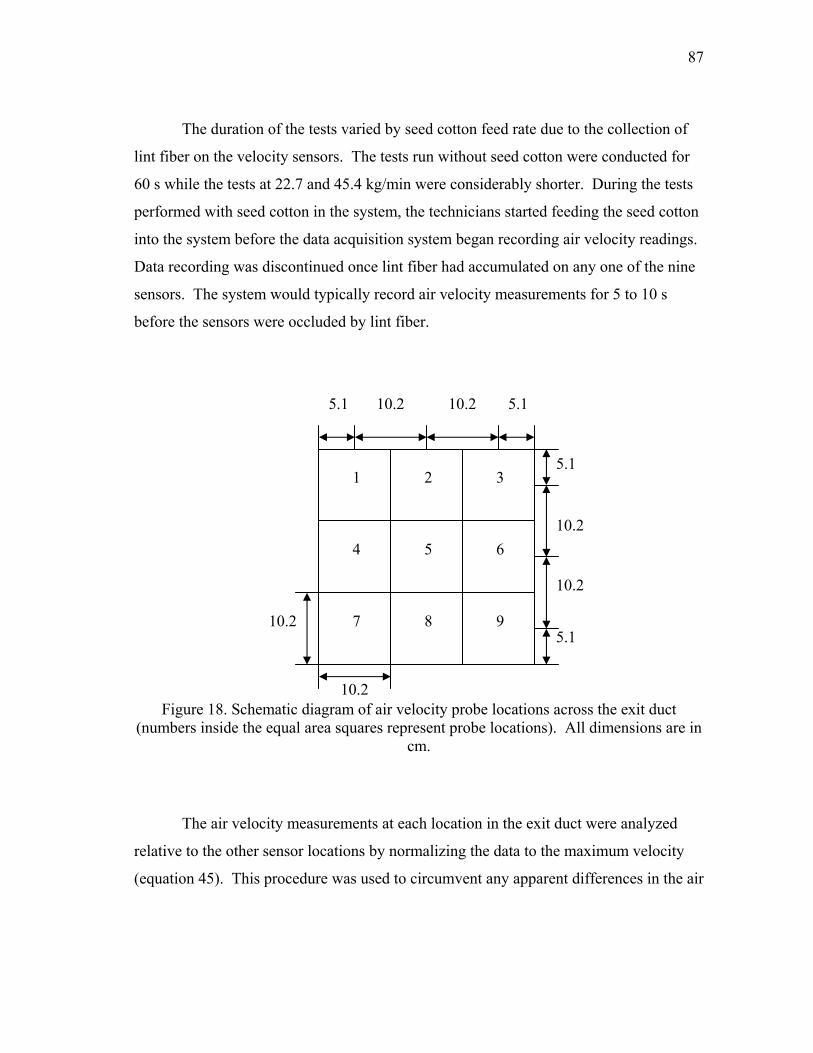
87
The duration of the tests varied by seed cotton feed rate due to the collection of
lint fiber on the velocity sensors. The tests run without seed cotton were conducted for
60 s while the tests at 22.7 and 45.4 kg/min were considerably shorter. During the tests
performed with seed cotton in the system, the technicians started feeding the seed cotton
into the system before the data acquisition system began recording air velocity readings.
Data recording was discontinued once lint fiber had accumulated on any one of the nine
sensors. The system would typically record air velocity measurements for 5 to 10 s
before the sensors were occluded by lint fiber.
Figure 18. Schematic diagram of air velocity probe locations across the exit duct (numbers inside the equal area squares represent probe locations). All dimensions are in
cm.
The air velocity measurements at each location in the exit duct were analyzed
relative to the other sensor locations by normalizing the data to the maximum velocity
(equation 45). This procedure was used to circumvent any apparent differences in the air
10.2
10.2
1 2 3
4 5 6
7 8 9
10.2
10.2
10.2 10.2
5.1
5.1
5.1 5.1
88
flow patterns between seed cotton feed rates due to the uncertainty associated with
measuring and controlling the system air flow rate.
100max
, ⎟⎟⎠
⎞⎜⎜⎝
⎛=
VVV i
in (45)
where Vn,i = normalized velocity of position i represented as a percentage of the
maximum velocity (%), Vi = air velocity measurement of sensor position i (m/s), and
Vmax = maximum air velocity measurement of the nine sensor positions in the exit duct
(m/s).
The normalized velocity data were analyzed in SPSS using the multivariate
analysis of variance (MANOVA) procedure in the General Linear Model algorithm to
test for overall differences in the air velocity patterns between seed cotton feed rates.
The test statistic used to evaluate the significance of the MANOVA test was Wilks’ λ
(Johnson and Wichern, 2002).
Concentration Profile Testing
Concentration profile testing in the exit duct was conducted using a five point
sampling grid with sampling locations as shown in Figure 19. The goal of this effort
was to determine the magnitude of an isokinetic emission concentration measured at the
center of the exit duct relative to the duct average concentration. The results of this
evaluation would then be used to correct center point concentration measurements to
duct average concentrations for use in calculating emission rates and subsequent
emission factors. The four sampling locations surrounding the center sampling location
were used to determine the average emission concentration in the exit duct.

89
Figure 19. Schematic diagram of concentration sampling locations in the exit duct
(numbers represent sampling locations). All dimensions are in cm.
A dust feeder was used to feed corn starch into the air stream at 12 g/min. The
dust feeding system was operated by a linear drive system powered by a 0.187 kW (1/4
hp) DC motor with an 80:1 speed reducing gear box. The linear drive system consisted
of a 1.8 m long, 2.54 cm diameter, 5 pitch Acme threaded shaft with two traveler nuts
attached to the 20.3 cm x 1.8 m dust table. The dust was spread out in a uniform depth
pattern (approximately 138 cm long by 5 cm wide) on top of the dust table. As the
threaded shaft was rotated by the motor (27 rpm), the dust table advanced passed a
venturi nozzle which pulled the dust from the table and introduced it into the air stream
passing into the inlet of the seed cotton feeding system (Figure 20).
1
2
4
5
3
15.2
15.2
15.2
15.2
7.6
7.6
7.6 7.6

90
Figure 20. Linear motion dust feeding system used to feed corn starch into the testing
system at 12 g/min.
The isokinetic sampling nozzles were constructed from 7.04 mm (0.277 in) inner
diameter seamless steel tubing with 1.24 mm (0.049 in) wall thickness. The sampling
nozzles were installed coplanar to one another at 20.3 cm (8 in) from the end of the exit
duct. The air flow rate through each sampling nozzle was measured with an orifice
meter and controlled using a manually operated ball valve. The pressure drop across
each orifice meter was monitored by a magnehelic gage and differential pressure
transducer (PX274, Omega Engineering, Inc., Stamford, Conn.) The flow rate through
each orifice meter was calculated using equation 3 and the differential pressure
measured across the orifice (orifice diameter = 4.763 mm = 0.1875 in).
The velocity of the air entering each of the sampling nozzles was calculated by
dividing the flow rate measured by the orifice meter by the inlet area of the nozzle
(0.389 cm2). The velocity of the air passing each nozzle was measured using an air
velocity probe (641RM-12, Dwyer Instruments, Inc., Michigan City, IN). Isokinetic
sampling conditions were maintained by regulating the sampler nozzle flow rate with the
manually operated ball valve. These two velocities were recorded along with air
temperature, relative humidity, and barometric pressure readings by the data acquisition
system used to record the air velocity profile data. Post test analysis of the air velocity

91
readings was conducted to determine how precisely isokinetic conditions were
maintained at the sampling nozzles using the EPA Method 5 (CFR, 1999) criteria.
These criteria state that the ratio of the air velocity entering the nozzle to the air velocity
passing the nozzle should be within 0.9 to 1.1 (CFR, 1999).
The airflow through each sampling nozzle was provided by a rotary vane vacuum
pump (1023-V131Q, Gast Mfg., Inc., Benton Harbor, MI). The sampled air was pulled
through the sampling nozzle and 47 mm diameter filter (2 μm pore size Zefluor
Membrane Filters, Pall Corp., East Hills, NY) where the particulate matter was separated
from the air stream. The filters were pre and post weighed using a high precision
analytical balance (AG245, Mettler-Toledo, Greifensee Switzerland). The pre and post
processing of the filters is described by Wanjura et al. (2005b). The concentration
measured at each location was calculated by dividing the net mass of accumulated PM
on the filter by the total air volume pulled through the filter during the test.
The system air flow rate was monitored and maintained at 85 m3/min (3000
ft3/min) during each of the tests. The system air flow rate was measured using a pitot
tube in the 12.7 cm (5 in) diameter ducts on the exit side of each fan. Five tests were
conducted at the 12 g/min nominal feed rate and the duration of each test was
approximately 10 min.
The concentration data was normalized using the maximum concentration
measured during each test to help identify concentration profile patterns. The ratio of
the duct average concentration to the center point concentration was calculated and used
in the concentration profile analysis. The univariate ANOVA procedure in the General
Linear Model algorithm in SPSS was used to analyze the normalized concentration data.
Particle size distribution (PSD) analyses of the raw corn starch and PM collected on the
filters were conducted on a Coulter Counter Multisizer3 according to the procedure
described by Faulkner and Shaw (2006). A particle density of 1.5 g/cm3, measured by
an AccuPyc 1330 Pycnometer (AccuPyc 1330 Pycnometer, Micromeritics Instrument
Corp., Norcross, GA), was used to convert the Equivalent Spherical Diameter PSDs

92
from the Coulter to an AED basis. The PSD data were analyzed to investigate
differences in PSD by sampling location within the exit duct.
Total System Deposition Testing
The source sampling system designed for use onboard the harvesting system was
mounted on the test frame along with the seed cotton separation system (see Figure 21)
to evaluate the total mass of dust lost to deposition within the system. The isokinetic
sampling system was modified from the 2006 design to include an automated control
system as well as improved sampling train duct work to minimize dust losses and
prevent plugging by locks of seed cotton penetrating the exit duct. The isokinetic nozzle
(diameter = 59.563 mm) mounted inside the exit duct was designed for a sampling
velocity of 732 ± 122 m/min based on onboard duct measurements from 2006. The
sampling flow rate (passing through the nozzle), based on the design inlet velocity of the
barrel cyclone, was specified at 2.124 m3/min (75 ft3/min). The airflow through the
system was provided for by two fans mounted in series (Model HP-33, Clements
National Company, Chicago, IL) and controlled by an automated ball valve
(PBVPV1206, Dwyer Instruments Inc., Michigan City, IN). The pressure drop across
the orifice meter and the velocity pressure measured by a pitot tube (Model 160-8,
Dwyer Instruments Inc., Michigan City, IN) mounted in the duct were measured by
pressure transducers (Series 677, Dwyer Instruments Inc., Michigan City, IN). Air
temperature and relative humidity as well as barometric pressure were measured inside
the duct using a T/RH probe (HX94A, Omega Engineering Inc., Stamford, CT) and
barometric pressure transmitter (Model 278, Setra Systems Inc., Boxborough, MA). The
measurement and control system (cFP-AI-110 input module, cFP-AO-200 output
module, National Instruments, Austin, TX) used with the source sampling system was
operated by a laptop computer running LabView 8.0 (LabView v. 8.0, National
Instruments, Austin, TX). The measurement and control system monitored and recorded
the readings from the pressure transducers, T/RH probe, and barometric pressure
93
transmitter and performed the calculations on a real-time basis for controlling the airflow
rate through the system on a 1 Hz frequency.
The particulate matter penetrating the cyclone was captured on a set of two, 20.3
by 25.4 cm coated borosilicate glass microfiber filters (Pall Corp., Pallflex Emfab filter
material 7224, East Hills, NY). The filters were pre and post weighed according to the
process described previously for the 47 mm diameter Teflon filters using a high
precision analytical balance (AG245, Mettler-Toledo, Greifensee Switzerland). The
cyclone bucket was pre and post weighed with a laboratory balance (PB1502, Mettler-
Toledo, Greifensee Switzerland).
Five replications at each of two dust feed rates (5 and 10 g/min) were conducted
with a target duct velocity of 732 m/min (2500 ft/min). Corn starch was used as the dust
in the tests. The total system deposition was calculated as shown in equation 46.
100*1 ⎟⎟⎠
⎞⎜⎜⎝
⎛−=
inmERD (46)
where D is the total system deposition (%), min is the calculated feeding rate of the dust
into the system (g/min), and ER is the total emission rate of dust from the exit duct as
calculated by the emission concentration measured by the source sampler multiplied by
the total duct flow rate (g/min).

94
Figure 21. Photograph of the source sampling system mounted on the test frame.
SYSTEM DEVELOPMENT AND EVALUATION RESULTS
Seed Cotton Separation System Evaluation
The seed cotton penetration test results for separator box design 1 with baffles 1,
2, and 3 (see Table 22) are shown in Table 23 and Figure 22. No significant interaction
was observed between the baffle and seed cotton feed rate factors (p value = 0.734).
However, an ANOVA on the seed cotton penetration data indicated significant
differences by baffle design (p value = 0.016) and by nominal seed cotton feed rate (p
value < 0.001). Significant differences (α = 0.05) were observed between the baffles at
the 45.4 and 68.1 kg/min feed rates according to Tukey’s HSD test (Table 23).
Although significant differences between the mass of seed cotton penetrating the system
was not observed between the 22.7 and 45.4 kg/min feed rates, the mean mass of seed
cotton penetrating the system at the 68.1 kg/min feed rate was significantly higher than
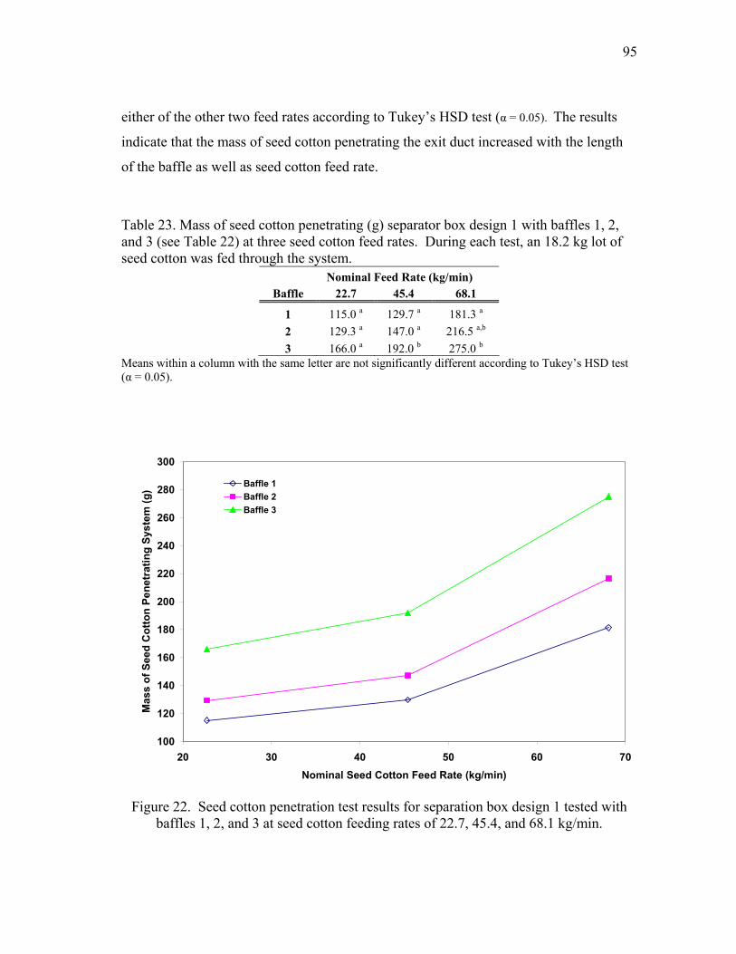
95
either of the other two feed rates according to Tukey’s HSD test (α = 0.05). The results
indicate that the mass of seed cotton penetrating the exit duct increased with the length
of the baffle as well as seed cotton feed rate.
Table 23. Mass of seed cotton penetrating (g) separator box design 1 with baffles 1, 2, and 3 (see Table 22) at three seed cotton feed rates. During each test, an 18.2 kg lot of seed cotton was fed through the system.
Nominal Feed Rate (kg/min) Baffle 22.7 45.4 68.1
1 115.0 a 129.7 a 181.3 a 2 129.3 a 147.0 a 216.5 a,b 3 166.0 a 192.0 b 275.0 b
Means within a column with the same letter are not significantly different according to Tukey’s HSD test (α = 0.05).
100
120
140
160
180
200
220
240
260
280
300
20 30 40 50 60 70Nominal Seed Cotton Feed Rate (kg/min)
Mas
s of
See
d C
otto
n Pe
netr
atin
g Sy
stem
(g) Baffle 1
Baffle 2Baffle 3
Figure 22. Seed cotton penetration test results for separation box design 1 tested with
baffles 1, 2, and 3 at seed cotton feeding rates of 22.7, 45.4, and 68.1 kg/min.
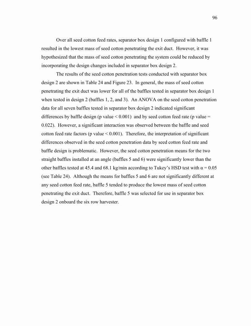
96
Over all seed cotton feed rates, separator box design 1 configured with baffle 1
resulted in the lowest mass of seed cotton penetrating the exit duct. However, it was
hypothesized that the mass of seed cotton penetrating the system could be reduced by
incorporating the design changes included in separator box design 2.
The results of the seed cotton penetration tests conducted with separator box
design 2 are shown in Table 24 and Figure 23. In general, the mass of seed cotton
penetrating the exit duct was lower for all of the baffles tested in separator box design 1
when tested in design 2 (baffles 1, 2, and 3). An ANOVA on the seed cotton penetration
data for all seven baffles tested in separator box design 2 indicated significant
differences by baffle design (p value < 0.001) and by seed cotton feed rate (p value =
0.022). However, a significant interaction was observed between the baffle and seed
cotton feed rate factors (p value < 0.001). Therefore, the interpretation of significant
differences observed in the seed cotton penetration data by seed cotton feed rate and
baffle design is problematic. However, the seed cotton penetration means for the two
straight baffles installed at an angle (baffles 5 and 6) were significantly lower than the
other baffles tested at 45.4 and 68.1 kg/min according to Tukey’s HSD test with α = 0.05
(see Table 24). Although the means for baffles 5 and 6 are not significantly different at
any seed cotton feed rate, baffle 5 tended to produce the lowest mass of seed cotton
penetrating the exit duct. Therefore, baffle 5 was selected for use in separator box
design 2 onboard the six row harvester.
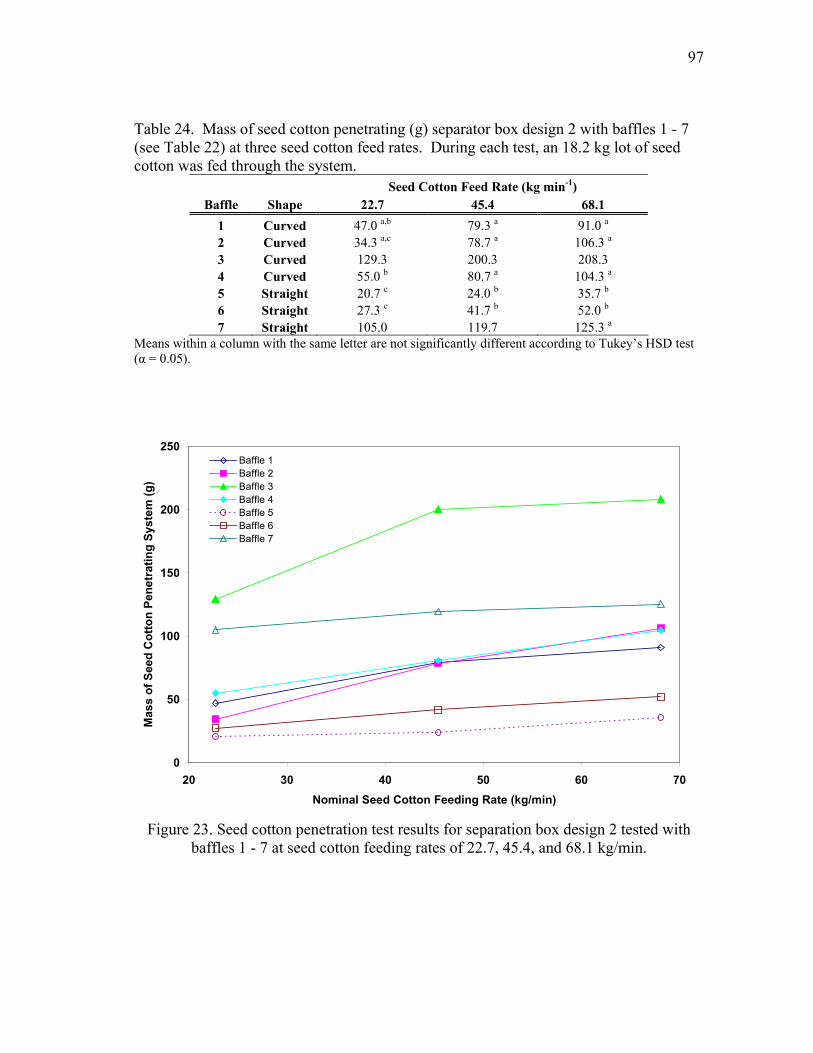
97
Table 24. Mass of seed cotton penetrating (g) separator box design 2 with baffles 1 - 7 (see Table 22) at three seed cotton feed rates. During each test, an 18.2 kg lot of seed cotton was fed through the system.
Seed Cotton Feed Rate (kg min-1) Baffle Shape 22.7 45.4 68.1
1 Curved 47.0 a,b 79.3 a 91.0 a 2 Curved 34.3 a,c 78.7 a 106.3 a 3 Curved 129.3 200.3 208.3 4 Curved 55.0 b 80.7 a 104.3 a
5 Straight 20.7 c 24.0 b 35.7 b 6 Straight 27.3 c 41.7 b 52.0 b 7 Straight 105.0 119.7 125.3 a
Means within a column with the same letter are not significantly different according to Tukey’s HSD test (α = 0.05).
0
50
100
150
200
250
20 30 40 50 60 70Nominal Seed Cotton Feeding Rate (kg/min)
Mas
s of
See
d C
otto
n Pe
netr
atin
g Sy
stem
(g)
Baffle 1Baffle 2Baffle 3Baffle 4Baffle 5Baffle 6Baffle 7
Figure 23. Seed cotton penetration test results for separation box design 2 tested with
baffles 1 - 7 at seed cotton feeding rates of 22.7, 45.4, and 68.1 kg/min.
98
Velocity Profile Testing
A MANOVA test performed on the normalized velocity data indicates that there
is no significant difference in the air velocity patterns between any of the seed cotton
feed rates (α = 0.05). The value of Wilks’ λ calculated in SPSS was 0.077 with an F
statistic value of 1.625 (p value = 0.220). An individual comparison of the normalized
velocities by sensor location (shown in Table 25) also indicate that there is little
difference in the air velocity patterns by seed cotton feed rate. Only probes three and
seven indicated significant differences between mean normalized air velocities between
seed cotton feed rates. However, these differences should be interpreted with caution
due to the insignificance of the MANOVA test. The results of the velocity profile tests
are shown in Table 25 and Figure 24.
Table 25. Mean normalized air velocity measurements (% of maximum duct velocity) from five replicated tests at three seed cotton feed rates. The probes were located coplanar to one another at nine evenly spaced points across the cross section of the exit duct (see Figure 18).
Seed Cotton Feed Rate (kg/min) Probe No. 0 22.7 45.4
1 82.6a 82.6a 82.6a 2 90.9a 90.7a 91.3a 3 82.2 a 82.5 a,b 83.3 b 4 83.2a 84.1a 83.6a 5 100.0a 100.0a 100.0a 6 93.6a 94.0a 94.4a 7 87.4a 88.5b 88.2a,b 8 98.4a 98.5a 98.5a 9 94.6a 94.3a 94.3a
Maximum Air
Velocity (m/min)
1078.8 1077.5 1077.7
Means within a row with the same letter are not significantly different according to Tukey’s HSD test (α = 0.05).

99
An ANOVA test on the normalized velocity data indicated significant differences
between the sensors for the 0 (p value < 0.001), 22.7 (p value < 0.001), and 45.4 kg/min
feed rates (p value < 0.001). Tukey’s HSD test indicated that the center point
normalized velocity was significantly different than at all other sensor locations for the 0
and 22.7 kg min-1 feed rates (α = 0.05). However, the same test indicated that the
normalized velocity at sensor locations five (center point) and eight were not
significantly different at the 45.4 kg/min feed rate. The air velocity profiles shown in
Figure 24 consistently indicate that the maximum air velocity in the exit duct is at the
center point (probe location 5). In addition, the velocity of the air in the exit duct
generally increases from the top to the bottom side.
70%
75%
80%
85%
90%
95%
100%
1 2 3 4 5 6 7 8 9Probe Position Number
Nor
mal
ized
Vel
ocity
(% o
f Max
imum
Vel
ocity
) No Seed Cotton22.7 kg/min45.4 kg/min
Figure 24. Normalized velocity measurements at nine coplanar points across the cross
section of the exit duct.
100
Concentration Profile Testing
The results of the concentration tests performed on the exit duct of the seed
cotton separation system are shown in Table 26 and Figure 25. An ANOVA test
indicated significant differences between mean concentrations by probe location (p value
= 0.005). The mean center point correction factor, calculated as the ratio of the duct
average concentration to the center point concentration, for all five tests was 93%. An
ANOVA test on the concentration data indicate that there is no significant difference
between the duct mean concentration and center point (probe location 3) concentration
measurements (p value = 0.248). Thus, an isokinetic concentration measurement taken
at the center point of the exit duct is likely to adequately represent the duct average
emission concentration.
Isokinetic sampling conditions were evaluated for each sampling probe using the
ratio of the air velocity entering the sampling probe to the air velocity passing the probe.
A summary of this ratio for each sampling probe during each test is shown in Table 27.
In general, isokinetic sampling conditions were consistently maintained for each sampler
during each test. However, during the first test, isokinetic sampling conditions were not
maintained for probe five for 93 s due to an equipment malfunction. An equipment
malfunction also resulted in the decreased sampling time for sampling probe one during
test one. Hinds (1999) describes the ratio of the probe concentration (Cp) to the free
stream concentration (Co) in the duct under anisokinetic sampling conditions as shown in
equation 47.

101
Table 26. Concentration data collected at five coplanar locations across the cross section of the exit duct of the seed cotton separation system.
Test Probe Location Concentration Relative
Concentration Center Point
Correction Factor Duct Mean
Concentration
(mg m-3) (% of Max Concentration) (%) (mg m-3)
1 1 71.9 76.3% 2 84.8 90.0% 3* 87.1 92.4% 87.5% 76.1 4 94.2 100.0% 5 53.6 56.9%
2 1 67.9 86.7% 2 73.5 93.9% 3* 72.8 93.0% 97.1% 70.6 4 78.3 100.0% 5 62.9 80.3%
3 1 79.3 100.0% 2 66.9 84.3% 3* 78.2 98.5% 87.4% 68.3 4 73.7 92.9% 5 53.4 67.3%
4 1 69.4 87.1% 2 67.0 84.1% 3* 63.2 79.3% 110.0% 69.5 4 79.7 100.0% 5 61.8 77.6%
5 1 66.5 88.1% 2 69.2 91.7% 3* 75.4 100.0% 87.2% 65.8 4 66.4 88.0% 5 61.0 80.9%
Means 1 71.0a,b 90.5% 2 72.3a,b 92.1% 3* 75.3b 96.0% 93.0% 70.1 4 78.5b 100.0%
5 58.5a 74.6% * Indicates center point probe location. Mean concentrations with the same letter are not significantly different according to Tukey’s HSD test (α = 0.05).

102
0
10
20
30
40
50
60
70
80
90
100
1 2 3 4 5
Test Number
Con
cent
ratio
n (m
g/m
3 )Duct Mean ConcentrationCenter Point Concentration
Figure 25. Comparison of the duct mean concentration to the center point concentration
by test.
( ) ⎟⎟⎠
⎞⎜⎜⎝
⎛++
−⎟⎠⎞
⎜⎝⎛ −+=
SUUUU
CC
o
o
o
P
62.0211111 (47)
where Uo = free stream air velocity in the duct (m/s), U = velocity of the air entering the
sampling nozzle (m/s), and S = Stokes number. The unitless Stokes number for the inlet
of the sampling nozzle is given by equation 48.
s
o
DU
Sτ
= (48)
103
where τ = particle relaxation time (s), and Ds = sampling nozzle diameter. Hinds (1999)
defines τ in terms of particle diameter (d) as shown in equation 49.
ηρ
τ18
2cp Cd
= (49)
where ρp = particle density (kg/m), Cc = Cunningham correction factor, and η = absolute
viscosity (Pa – s).
The procedure described by Hinds (1999) was used on a time weighted average
basis (equation 50) with the PSD of the PM captured by sampling probe five during test
one to estimate the error in the concentration measurement resulting from the
anisokinetic sampling conditions. This analysis indicated that the measured
concentration was 3% greater than the free stream concentration in the duct at the
location of probe 5. Thus, the measurement error resulting from the anisokinetic
sampling conditions was considered to be negligible and the measured concentration
from probe five was used as reported for all analyses.
moia CCFCF =+ (50)
where Fa = fraction of sampling time when conditions were anisokinetic, Fi = fraction of
sampling time when conditions were isokinetic, and Cm = measured concentration
(μg/m3).

104
Table 27. Summary statistics for the ratio of the air velocity entering the sampling probe to the air velocity passing the probe calculated for five samplers during five concentration tests.
I = Nozzle Velocity / Probe Velocity Test Location Mean St. Dev. Min Max N (s)
Anisokinetic Time (s)
1 1 0.985 0.041 0.856 1.177 589 8 1 2 1.003 0.021 0.814 1.071 641 9 1 3 0.992 0.010 0.968 1.056 641 0 1 4 0.997 0.025 0.934 1.043 641 0 1 5 0.941 0.036 0.839 1.004 547 93
2 1 1.017 0.016 0.989 1.162 666 6 2 2 0.993 0.013 0.957 1.061 666 0 2 3 0.993 0.012 0.966 1.056 666 0 2 4 0.995 0.018 0.941 1.041 666 0 2 5 0.988 0.011 0.943 1.029 666 0
3 1 1.015 0.018 0.985 1.200 643 4 3 2 0.987 0.012 0.944 1.024 643 0 3 3 0.990 0.015 0.945 1.079 643 0 3 4 0.989 0.017 0.942 1.039 643 0 3 5 0.982 0.015 0.938 1.009 643 0
4 1 1.015 0.015 0.972 1.113 649 3 4 2 0.995 0.009 0.970 1.048 649 0 4 3 0.999 0.010 0.969 1.032 649 0 4 4 0.994 0.008 0.967 1.018 649 0 4 5 0.994 0.008 0.975 1.024 649 0
5 1 1.014 0.018 0.965 1.245 649 3 5 2 1.002 0.007 0.958 1.041 649 0 5 3 0.999 0.012 0.965 1.038 649 0 5 4 0.992 0.011 0.967 1.068 649 0 5 5 0.991 0.011 0.956 1.019 649 0
Particle Size Distribution Analysis
The AED MMD and GSD of the best fit lognormal distribution for each
isokinetic sampling probe location are shown in Table 28 along with the mass weighed
average PSD representing the duct average PSD. Also shown in Table 28 are the PSD
analysis results of the corn starch fed into the system during each test. The mass
105
weighted average PSD was calculated using the PSDs and net filter masses from the
sampling probes at locations 1, 2, 4, and 5 (see Figure 26). No significant differences (α
= 0.05) were observed between the MMD or GSD values for any of the sampling
locations (MMD p value = 0.749, GSD p value = 0.054). Further analysis indicated no
significant difference between the MMD of the mass weighted average PSD and the
center point location PSD (p value = 0.780). However, a significant difference between
the GSD values for the mass weighted average PSD and the center point location PSD
was observed (p value = 0.038). The difference in mean GSD values for the mass
weighted average and center point location PSDs is 0.06 (1.45 – 1.39 = 0.06). Although
this difference is significant, no appreciable difference between the duct mean and center
point PSDs was observed. The center point, mass weighted average, and inlet corn
starch PSDs measured for test 4 are shown in Figure 26. The overlapping of the three
PSDs shown in Figure 26 was typical of all the tests. The mean AED MMD and GSD of
the PSD for the corn starch used in the tests were 18.4 μm and 1.36, respectively. No
significant difference was observed between the mean MMD values for the inlet corn
starch, center point sampling location, and mass weighted average PSDs (p value =
0.109). However, significant differences in the GSD values from these PSDs were
observed (p value = 0.008). Further analysis using Tukey’s HSD test indicated that two
homogeneous subsets exist in the GSD values using the data taken from the inlet corn
starch, center point sampling location, and mass weighted average PSDs. The
constituents within each homogeneous subset are not significantly different while
significant differences exist between subsets. The constituents of subset one were the
inlet cornstarch and center point sampling location GSDs (p value = 0.494) while the
second subset was made up by the GSD values from the center point sampling location
and mass weighted average PSDs (p value = 0.059). These results indicate that the PSD
of the inlet dust was not substantially altered between the feeding point and exit of the
seed cotton separation system.
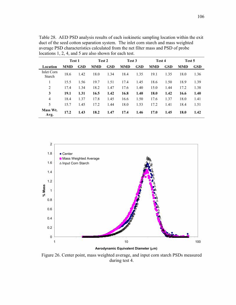
106
Table 28. AED PSD analysis results of each isokinetic sampling location within the exit duct of the seed cotton separation system. The inlet corn starch and mass weighted average PSD characteristics calculated from the net filter mass and PSD of probe locations 1, 2, 4, and 5 are also shown for each test. Test 1 Test 2 Test 3 Test 4 Test 5 Location MMD GSD MMD GSD MMD GSD MMD GSD MMD GSD Inlet Corn
Starch 18.6 1.42 18.0 1.34 18.4 1.35 19.1 1.35 18.0 1.36
1 15.5 1.56 19.7 1.51 17.4 1.45 18.6 1.50 18.9 1.39 2 17.4 1.34 18.2 1.47 17.6 1.40 15.0 1.44 17.2 1.38 3 19.1 1.31 16.5 1.42 16.8 1.40 18.0 1.42 16.6 1.40 4 18.4 1.37 17.8 1.45 16.6 1.50 17.6 1.37 18.0 1.41 5 15.7 1.45 17.2 1.44 18.0 1.53 17.2 1.41 18.4 1.51
Mass Wt. Avg. 17.2 1.43 18.2 1.47 17.4 1.46 17.0 1.45 18.0 1.42
0
0.2
0.4
0.6
0.8
1
1.2
1.4
1.6
1.8
2
1 10 100
Aerodynamic Equivalent Diameter (μm)
% M
ass
CenterMass Weighted AverageInput Corn Starch
Figure 26. Center point, mass weighted average, and input corn starch PSDs measured
during test 4.
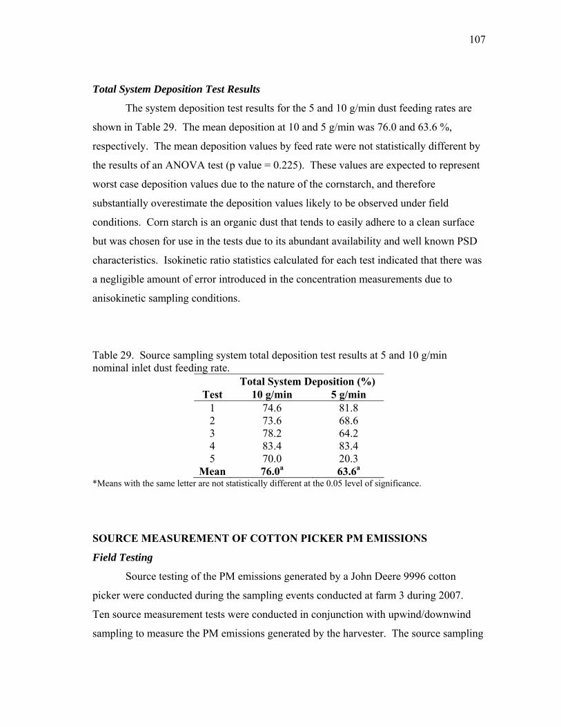
107
Total System Deposition Test Results
The system deposition test results for the 5 and 10 g/min dust feeding rates are
shown in Table 29. The mean deposition at 10 and 5 g/min was 76.0 and 63.6 %,
respectively. The mean deposition values by feed rate were not statistically different by
the results of an ANOVA test (p value = 0.225). These values are expected to represent
worst case deposition values due to the nature of the cornstarch, and therefore
substantially overestimate the deposition values likely to be observed under field
conditions. Corn starch is an organic dust that tends to easily adhere to a clean surface
but was chosen for use in the tests due to its abundant availability and well known PSD
characteristics. Isokinetic ratio statistics calculated for each test indicated that there was
a negligible amount of error introduced in the concentration measurements due to
anisokinetic sampling conditions.
Table 29. Source sampling system total deposition test results at 5 and 10 g/min nominal inlet dust feeding rate.
Total System Deposition (%) Test 10 g/min 5 g/min
1 74.6 81.8 2 73.6 68.6 3 78.2 64.2 4 83.4 83.4 5 70.0 20.3
Mean 76.0a 63.6a *Means with the same letter are not statistically different at the 0.05 level of significance.
SOURCE MEASUREMENT OF COTTON PICKER PM EMISSIONS
Field Testing
Source testing of the PM emissions generated by a John Deere 9996 cotton
picker were conducted during the sampling events conducted at farm 3 during 2007.
Ten source measurement tests were conducted in conjunction with upwind/downwind
sampling to measure the PM emissions generated by the harvester. The source sampling

108
system was installed on the harvester on duct 3 in the same configuration in which it was
tested (see previous discussion of source sampling system testing and evaluation). Each
test plot was setup so that the harvester made a total of eight passes in the field (4
rounds) covering 48 rows per test. The test plots ranged in size from 2.3 to 1.01 ha and
the test durations ranged from 128 to 49 min. The 20.3 x 25.4 cm filters used in the
source sampler (Pall Corp., Pallflex Emfab filter material 7224, East Hills, NY) were pre
and post weighed according to the previously discussed procedure for weighing 47 mm
diameter filters for the low volume TSP samplers. A total of four filters were used
during each test at farm 3. The two filters initially installed in the source sampling filter
bank were replaced half way through each test to prevent overloading. The cyclone
bucket was weighed prior to and after each test using a laboratory balance (PB1502,
Mettler-Toledo, Greifensee Switzerland).
Prior to entering the field, the system operator would start the fan on the
harvester and run the picker engine at full throttle to allow the system to stabilize before
entering the field. Once the harvester fan was running at full speed, the operator
switched on the source sampler fans through the laptop computer and allowed the source
sampling system to equilibrate with the harvester air system before entering the field.
Typically this warm-up process would last approximately 10-15 s. The harvester speed
was held approximately constant in the field at 6.44 km/h. Thus the load on the
harvester would vary by yield and plant density resulting in fluctuations in the harvester
fan speed. Typically, these fluctuations were brief in nature only lasting a few seconds.
Therefore, the control algorithm used in the source sampler control system was
configured to modulate the valve position based on a 7 second running average for both
the exit duct velocity and source sampler nozzle velocity. The duct velocity was
measured by a pitot tube (Model 160-8, Dwyer Instruments Inc., Michigan City, IN)
mounted 2.5 cm to the side of the sampling nozzle mounted in the center of the duct.
The velocity of the air entering the sampler nozzle was calculated by dividing the flow
rate through the orifice meter by the cross sectional area of the nozzle. The tip of the
sampling nozzle and pitot tube were mounted at the same distance inward from the exit
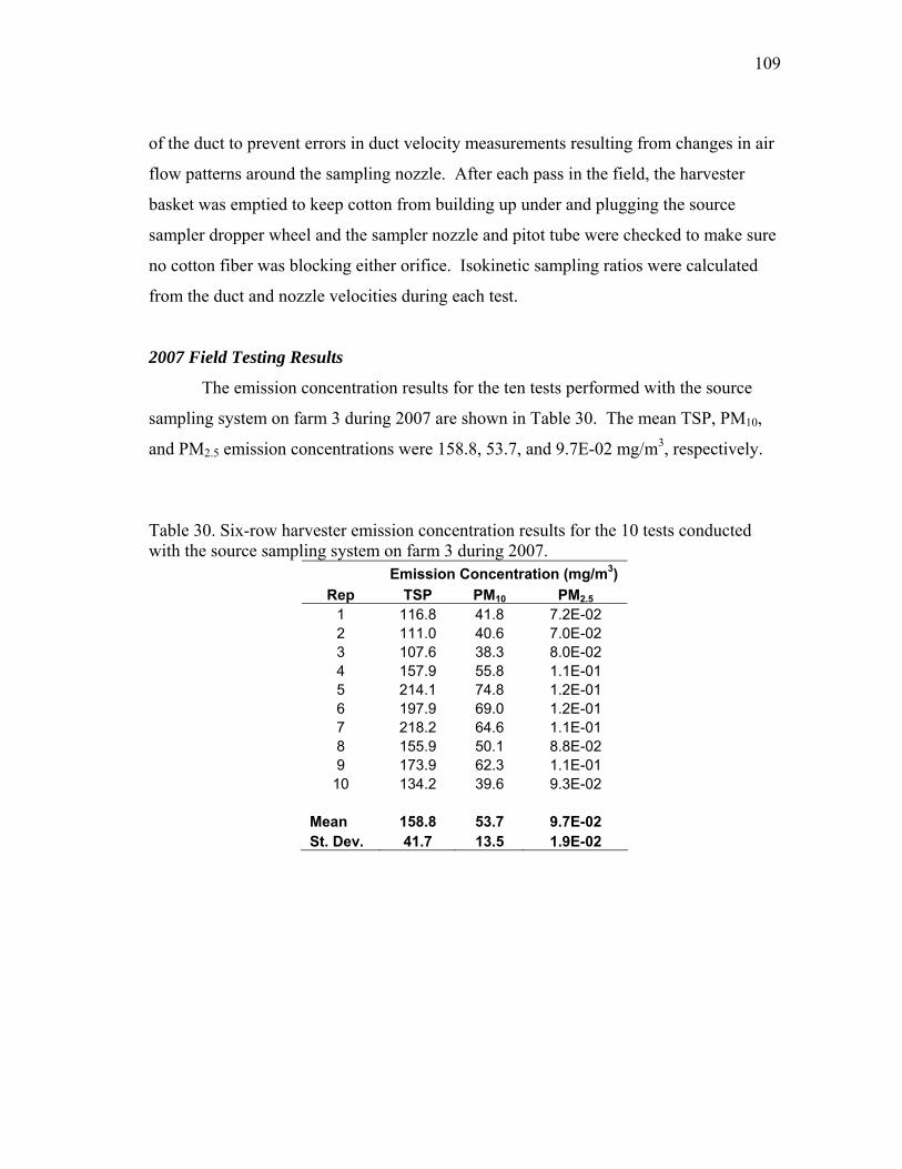
109
of the duct to prevent errors in duct velocity measurements resulting from changes in air
flow patterns around the sampling nozzle. After each pass in the field, the harvester
basket was emptied to keep cotton from building up under and plugging the source
sampler dropper wheel and the sampler nozzle and pitot tube were checked to make sure
no cotton fiber was blocking either orifice. Isokinetic sampling ratios were calculated
from the duct and nozzle velocities during each test.
2007 Field Testing Results
The emission concentration results for the ten tests performed with the source
sampling system on farm 3 during 2007 are shown in Table 30. The mean TSP, PM10,
and PM2.5 emission concentrations were 158.8, 53.7, and 9.7E-02 mg/m3, respectively.
Table 30. Six-row harvester emission concentration results for the 10 tests conducted with the source sampling system on farm 3 during 2007.
Emission Concentration (mg/m3) Rep TSP PM10 PM2.5
1 116.8 41.8 7.2E-02 2 111.0 40.6 7.0E-02 3 107.6 38.3 8.0E-02 4 157.9 55.8 1.1E-01 5 214.1 74.8 1.2E-01 6 197.9 69.0 1.2E-01 7 218.2 64.6 1.1E-01 8 155.9 50.1 8.8E-02 9 173.9 62.3 1.1E-01
10 134.2 39.6 9.3E-02 Mean 158.8 53.7 9.7E-02 St. Dev. 41.7 13.5 1.9E-02

110
Emission rates for each test were calculated by multiplying the measured
emission concentrations by the calculated average duct flow rate. The resulting emission
rates are shown in Table 31. The emission rate data appear to trend with the emission
factor results from the dispersion modeling process using both ISCST3 and AERMOD.
Table 31. Six-row harvester emission rates for ten tests conducted with the source sampling system on farm 3 during 2007.
Emission Rate (g/min) Rep TSP PM10 PM2.5
1 50.9 18.2 0.031 2 43.3 15.8 0.027 3 44.6 15.9 0.033 4 67.4 23.8 0.045 5 88.0 30.8 0.051 6 85.6 29.8 0.051 7 91.5 27.1 0.044 8 66.8 21.5 0.038 9 75.0 26.9 0.050 10 57.7 17.0 0.040
Mean* 67.1 ± 11.05 22.7 ± 3.59 0.041 ± 0.005 St. Dev. 17.8 5.8 0.009
*Means are shown with 95% confidence intervals.
An analysis of the systematic uncertainty for the source sampling system was
conducted according to the procedure described by Kline and McClintock (1953) and
used by Price (2004). The average uncertainty due to systematic effects for the source
sampler was determined to be 2.78%. A subsequent sensitivity analysis indicated that
the majority of the overall systematic uncertainty was due to the measurement of the
airflow rate, more specifically in the measurement of pressure drop across the orifice
meter in the calibration process. The same sensitivity analysis result was observed by
Price (2004) for the low volume TSP samplers. The results of this analysis are presented
in Appendix E.
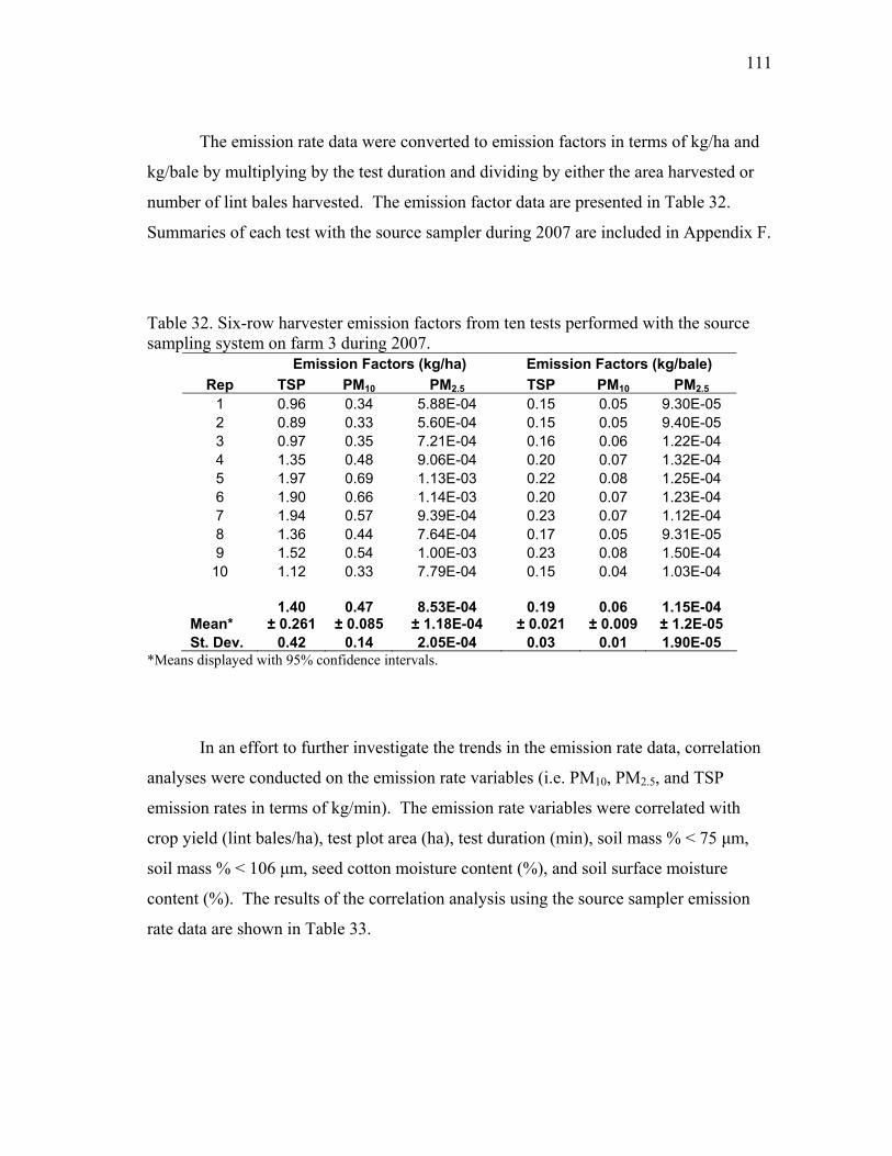
111
The emission rate data were converted to emission factors in terms of kg/ha and
kg/bale by multiplying by the test duration and dividing by either the area harvested or
number of lint bales harvested. The emission factor data are presented in Table 32.
Summaries of each test with the source sampler during 2007 are included in Appendix F.
Table 32. Six-row harvester emission factors from ten tests performed with the source sampling system on farm 3 during 2007.
Emission Factors (kg/ha) Emission Factors (kg/bale) Rep TSP PM10 PM2.5 TSP PM10 PM2.5
1 0.96 0.34 5.88E-04 0.15 0.05 9.30E-05 2 0.89 0.33 5.60E-04 0.15 0.05 9.40E-05 3 0.97 0.35 7.21E-04 0.16 0.06 1.22E-04 4 1.35 0.48 9.06E-04 0.20 0.07 1.32E-04 5 1.97 0.69 1.13E-03 0.22 0.08 1.25E-04 6 1.90 0.66 1.14E-03 0.20 0.07 1.23E-04 7 1.94 0.57 9.39E-04 0.23 0.07 1.12E-04 8 1.36 0.44 7.64E-04 0.17 0.05 9.31E-05 9 1.52 0.54 1.00E-03 0.23 0.08 1.50E-04
10 1.12 0.33 7.79E-04 0.15 0.04 1.03E-04
Mean* 1.40
± 0.261 0.47
± 0.085 8.53E-04
± 1.18E-04 0.19
± 0.021 0.06
± 0.009 1.15E-04 ± 1.2E-05
St. Dev. 0.42 0.14 2.05E-04 0.03 0.01 1.90E-05 *Means displayed with 95% confidence intervals.
In an effort to further investigate the trends in the emission rate data, correlation
analyses were conducted on the emission rate variables (i.e. PM10, PM2.5, and TSP
emission rates in terms of kg/min). The emission rate variables were correlated with
crop yield (lint bales/ha), test plot area (ha), test duration (min), soil mass % < 75 μm,
soil mass % < 106 μm, seed cotton moisture content (%), and soil surface moisture
content (%). The results of the correlation analysis using the source sampler emission
rate data are shown in Table 33.

112
Table 33. Correlation results of the source sampler emission rate data with area, yield, test duration, soil mass % < 75 μm, soil mass % < 106 μm, seed cotton moisture content, and soil surface moisture content. Emission Rate (g/min) TSP PM10 PM2.5
R -0.503 -0.379 -0.611 Area (ha) p value 0.1382 0.2795 0.0605
R 0.850 0.775 0.718 Yield (bales/ha)* p value 0.0018 0.0085 0.0194
R -0.539 -0.425 -0.682 Duration (min) p value 0.1080 0.2203 0.0298
R -0.460 -0.377 -0.086 Soil Mass % < 75 μm p value 0.1815 0.2832 0.8129
R -0.334 -0.272 0.070 Soil Mass % < 106 μm p value 0.3458 0.4471 0.8473
R -0.005 -0.168 -0.028 Seed Cotton Moisture Content (%) p value 0.9885 0.6427 0.9384
R 0.018 -0.071 -0.153 Soil Surface Moisture Content (%) p value 0.9610 0.8448 0.6725
*Highlighted correlation coefficients are statistically significant at the 0.01 level of significance.
Significant correlations at the 0.01 level were observed in the relationships
between TSP and PM10 emission rates with yield. The PM2.5 emission rate correlation
with yield is significant at the 0.05 level. Poor correlations with test plot area were
observed for the emission rate data for any size indicator. These results indicate that PM
emission rates are more closely related with the mass of material processed through the
harvester on a unit area basis (i.e. yield) than with land area alone. Therefore it is
appropriate to list PM emission factors for cotton harvesting on a mass of PM emitted
per lint bale harvested basis.
Summary of Source Sampler Emission Factors
Source measurement of emission concentration onboard a six-row cotton picker
was successfully conducted during 2007. However, the novel system and protocol used
to develop PM emission factors through direct measurement was initially met with
skepticism. Some argued the following points:

113
• The system initially proposed to separate the seed cotton from the air
stream would significantly alter the performance of the harvesting
machine in the field and would be problematic from a safety and
performance standpoint.
• The system used to measure the emissions from the harvester would
alter the normal operating characteristics of the harvester air system and
would not be representative of normal operating conditions.
• Source measurements of PM emissions from the harvester basket do not
account for PM emissions generated by the interaction of the harvester
wheels and the soil surface.
The seed cotton separation system was designed to separate the maximum
amount of seed cotton from the air stream while minimizing the total pressure loss
added to the harvester air system. Measurements of the system pressure loss were
taken during the tests conducted to evaluate the seed cotton separation efficiency, air
velocity profile in the exit duct, and concentration profile in the exit duct. The results
of these measurements indicate that the system pressure loss at 71 m3/min (2500
ft3/min) and 85 m3/min (3000 ft3/min) were 20 cm H2O (8 in H20) 23 and cm H2O (9 in
H2O), respectively. The increased pressure loss through the system decreased the
velocity of the air in the seed cotton transport duct on the harvester from
approximately 1524 m/min (5000 ft/min) to approximately 915 m/min (3000 ft/min).
This decrease in air velocity did not result in operational problems with the harvester
in terms of plugging of air ducts, decreased picking efficiency, or safety issues.
The seed cotton separation system provided a means by which to remove the
seed cotton from the air stream and channel the particulate laden air stream to the back
of the harvester, providing a location from which to collect emission concentration
measurements. The seed cotton separation system effectively altered the airflow
patterns inside the basket in two ways:
1. The presence of the separation system in the basket created an obstacle around
which the airflow from the other seed cotton transport ducts must pass.

114
Anecdotally, this created additional turbulence in the basket potentially
increasing the entrainment and emission of PM from the harvester basket.
Additionally, the air exiting the exit duct on the seed cotton separation system
was directed perpendicular to the back wall of the basket with a separation
distance of approximately 30.5 cm (12 in) between the exit of the duct and the
back wall. This configuration essentially created a high velocity jet of air at
the rear of the harvester basket that normally is not there.
2. The particulate laden air carrying the seed cotton into the basket must normally
pass through a set of finger grates or through the screen panels on the side of
the basket in order to exit the system. In this process, an unspecified amount
of filtration takes place as the air passes through the lint fiber collected on the
finger grates and basket screen panels.
Evidence of the increased emissions due to the presence of the source sampler
can be seen in the significant differences observed between the mean emission factors
for the 6-row and 6-row w/ss treatments developed using both ISCST3 and AERMOD
during the sampling at farm 3 in 2007. Thus, the final emission factor for the six row
harvester developed through the dispersion modeling procedure with ISCST3 or
AERMOD is not inclusive of the emission factors from the 6-row w/ss treatment.
The emissions from duct 3 do not undergo the filtering process before the
emission concentrations are measured. Thus emission concentrations measured in the
exit duct could be considered higher than emission concentrations on the outside of the
harvester basket. Therefore, the PM emission factors developed from the source
sampling techniques described here have been developed from the measured emission
rates with no correction made to account for deposition. The emission factors from the
source sampling technique are not corrected for deposition according to the following
logic:
• The deposition values reported here substantially overstate the true
deposition in the field because the corn starch used in the tests does not
accurately mimic the nature of the primary silica based material
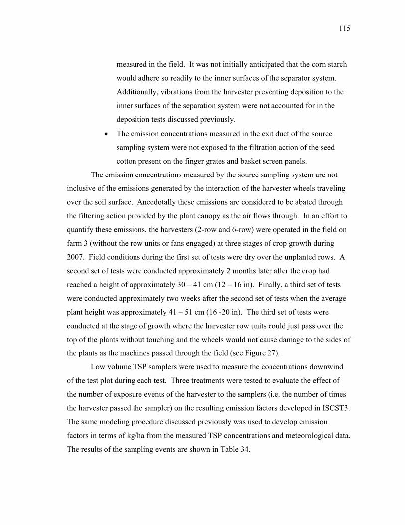
115
measured in the field. It was not initially anticipated that the corn starch
would adhere so readily to the inner surfaces of the separator system.
Additionally, vibrations from the harvester preventing deposition to the
inner surfaces of the separation system were not accounted for in the
deposition tests discussed previously.
• The emission concentrations measured in the exit duct of the source
sampling system were not exposed to the filtration action of the seed
cotton present on the finger grates and basket screen panels.
The emission concentrations measured by the source sampling system are not
inclusive of the emissions generated by the interaction of the harvester wheels traveling
over the soil surface. Anecdotally these emissions are considered to be abated through
the filtering action provided by the plant canopy as the air flows through. In an effort to
quantify these emissions, the harvesters (2-row and 6-row) were operated in the field on
farm 3 (without the row units or fans engaged) at three stages of crop growth during
2007. Field conditions during the first set of tests were dry over the unplanted rows. A
second set of tests were conducted approximately 2 months later after the crop had
reached a height of approximately 30 – 41 cm (12 – 16 in). Finally, a third set of tests
were conducted approximately two weeks after the second set of tests when the average
plant height was approximately 41 – 51 cm (16 -20 in). The third set of tests were
conducted at the stage of growth where the harvester row units could just pass over the
top of the plants without touching and the wheels would not cause damage to the sides of
the plants as the machines passed through the field (see Figure 27).
Low volume TSP samplers were used to measure the concentrations downwind
of the test plot during each test. Three treatments were tested to evaluate the effect of
the number of exposure events of the harvester to the samplers (i.e. the number of times
the harvester passed the sampler) on the resulting emission factors developed in ISCST3.
The same modeling procedure discussed previously was used to develop emission
factors in terms of kg/ha from the measured TSP concentrations and meteorological data.
The results of the sampling events are shown in Table 34.

116
Figure 27. Photograph of the six row harvester traveling down rows of cotton (average plant height 41 – 51 cm) with the row units and fan not engaged in order to measure the concentration of PM generated by the interaction of the harvester wheels and the soil surface (samplers located to the left of the harvester).
Replicated tests were not conducted during the first set of tests. The first set of
tests was conducted on fallow ground to determine if the emissions generated by the
wheel/soil surface interaction could be measured. With positive results from the first
tests, the second set of tests were conducted with replication but wind direction variation
within the tests resulted in invalid emission factor means for replications two and three,
leaving only the emission factors from replication one. The third set of tests was
conducted with three replications and the mean emission factors presented are the
average of all three replications. PM10 and PM2.5 emission factors were developed by
multiplying the respective TSP emission factor by the mass % PM10 and PM2.5 from the
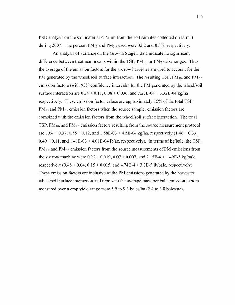
117
PSD analysis on the soil material < 75μm from the soil samples collected on farm 3
during 2007. The percent PM10 and PM2.5 used were 32.2 and 0.3%, respectively.
An analysis of variance on the Growth Stage 3 data indicate no significant
difference between treatment means within the TSP, PM10, or PM2.5 size ranges. Thus
the average of the emission factors for the six row harvester are used to account for the
PM generated by the wheel/soil surface interaction. The resulting TSP, PM10, and PM2.5
emission factors (with 95% confidence intervals) for the PM generated by the wheel/soil
surface interaction are 0.24 ± 0.11, 0.08 ± 0.036, and 7.27E-04 ± 3.32E-04 kg/ha
respectively. These emission factor values are approximately 15% of the total TSP,
PM10 and PM2.5 emission factors when the source sampler emission factors are
combined with the emission factors from the wheel/soil surface interaction. The total
TSP, PM10, and PM2.5 emission factors resulting from the source measurement protocol
are 1.64 ± 0.37, 0.55 ± 0.12, and 1.58E-03 ± 4.5E-04 kg/ha, respectively (1.46 ± 0.33,
0.49 ± 0.11, and 1.41E-03 ± 4.01E-04 lb/ac, respectively). In terms of kg/bale, the TSP,
PM10, and PM2.5 emission factors from the source measurements of PM emissions from
the six row machine were 0.22 ± 0.019, 0.07 ± 0.007, and 2.15E-4 ± 1.49E-5 kg/bale,
respectively (0.48 ± 0.04, 0.15 ± 0.015, and 4.74E-4 ± 3.3E-5 lb/bale, respectively).
These emission factors are inclusive of the PM emissions generated by the harvester
wheel/soil surface interaction and represent the average mass per bale emission factors
measured over a crop yield range from 5.9 to 9.3 bales/ha (2.4 to 3.8 bales/ac).
118
Table 34. Emission factors developed using measured TSP concentrations and ISCST3 for tests conducted to quantify the PM emissions generated by the interaction between the harvester wheels and the soil surface.
Growth Stage 1*
Pre-planting Growth Stage 2**
Plant Height: 30 - 41 cm Growth Stage 3***
Plant Height: 41 - 51 cm TSP PM10 PM2.5 TSP PM10 PM2.5 TSP+ PM10
+ PM2.5+
Treatment (kg/ha) (kg/ha) (kg/ha) (kg/ha) (kg/ha) (kg/ha) (kg/ha) (kg/ha) (kg/ha) 2 Row over 12 rows 5.84 1.88 1.75E-02 n/a n/a n/a 0.53a 0.17b 1.58E-03c
2 Row over 24 rows 9.31 3.00 2.79E-02 1.19 0.38 3.58E-03 0.45a 0.15b 1.36E-03c
2 Row over 36 rows 7.81 2.52 2.34E-02 0.57 0.18 1.71E-03 0.43a 0.14b 1.28E-03c
6 Row over 12 rows 4.26 1.37 1.28E-02 0.12 0.04 3.65E-04 0.31a 0.10b 9.43E-04c
6 Row over 24 rows 3.47 1.12 1.04E-02 0.51 0.16 1.52E-03 0.15a 0.05b 4.64E-04c
6 Row over 36 rows 12.54 4.04 3.76E-02 0.52 0.17 1.55E-03 0.26a 0.08b 7.74E-04c
+Means with the same letter are not significantly different at the 0.05 level of significance. *Replicated tests were not conducted at growth stage one. **Means displayed for Growth Stage 2 represent the mean emission factor from replication one due to variable wind directions during replications two and three. ***Means displayed for Growth Stage 3 represent the average of three replications per treatment.
119
CHAPTER V
PARTICLE SIZE DISTRIBUTION AND PARTICLE DENSITY ANALYSIS OF
PARTICULATE MATTER SAMPLES
INTRODUCTION
The analysis of particle size in terms of percent mass versus particle diameter
plays a key role in understanding both the nature of PM emissions as well as the
expected operating performance for sampling devices used to measure PM
concentrations. Buser (2004) concluded that significant errors result in PM
concentrations measured by FRM PM10 and PM2.5 samplers when exposed to PM with
aerodynamic mass median diameter larger than the cutpoint of the sampler. The
cutpoints of FRM PM10 and PM2.5 samplers are 10 and 2.5 μm respectively. Buser
(2004) further explains that these errors are a consequence of the interaction between the
sampler performance characteristics and the particle size distribution of the sampled PM.
The findings of Buser (2004) were based on theoretical simulations assuming that the
performance characteristics of the FRM PM10 and PM2.5 samplers remain constant
within specified performance criteria specified by EPA. Wanjura et al. (2005a) indicate
that the errors identified by Buser (2004) may be exacerbated by shifting of the
performance characteristics of PM10 samplers under field conditions.
A more appropriate basis for determining true PM2.5 and PM10 concentrations
was described by Buser (2004). The procedure described by Buser (2004) determines
true PM10 and PM2.5 concentrations by multiplying measured TSP concentrations by
mass fractions of PM10 or PM2.5 from subsequent particle size distribution analyses on
the TSP filters. The underlying premise of this procedure is that TSP concentrations
accurately represent the total concentration of suspended PM in the atmosphere since the
cutpoint of the TSP sampler is much larger than the MMD of the PM suspended in the
ambient air. McFarland and Ortiz (1983) indicate that the cutpoint of the TSP sampler is
on the order of 45 μm with a slope of 1.5. This procedure was used in this work to
determine accurate PM emission factors in terms of PM10, and PM2.5. The following
120
discussions describe the methods used to characterize the PM sampled from the cotton
harvesting operation with respect to particle density and particle size distribution.
METHODS
Particle size analyses were conducted on PM and soil samples to determine the
distribution of percent mass versus particle diameter. A Coulter Counter Multisizer III
(Beckman – Coulter, Coulter Multisizer III, Miami, FL) was used to determine an
estimate of the PSD for the different materials in terms of percent volume versus
equivalent spherical particle diameter (ESD) according to the procedure described by
Buser (2004). Prior to each analysis in the Coulter instrument, the sample was
suspended in a 5% LiCl – Methanol electrolyte solution and exposed to ultrasonic
vibration for fifteen min. The ultrasonic vibration provided the energy necessary to
remove captured PM from filter media as well as to separate agglomerated particles.
After the exposure to ultrasonic vibration, the technician transferred (via plastic pipette)
the PM/electrolyte solution to a beaker (located inside the Multisizer III) containing
approximately 50 ml of clean electrolyte until the concentration in the beaker reached
approximately 5%. Once the concentration in the beaker was sufficient, the technician
initiated the run. During each run, the instrument drew approximately 300,000 particles
through the aperture tube. An aperture tube with measurement range from 2 – 100 μm
was used. The effective maximum particle diameter measured by the Coulter is only
60% of the maximum aperture diameter, or in this case 60 μm. The aperture tube
contains two electrodes; between which flows a constant electrical current. When a
particle enters the aperture orifice, the momentary increase in impedance (due to the
presence of the particle) causes the electrical current flowing between the electrodes to
decrease. The increased impedance causes the portion of current not passing between
the two aperture electrodes to pass to an amplifier which converts the current pulse into a
voltage pulse. The Coulter Principle states that the amplitude of this voltage pulse is
directly proportional to the volume of the particle (Beckman Coulter, 2002). The
121
analysis of several hundred thousand particles allows for the development of a relative
frequency histogram relating percent volume to ESD.
A PSD based on percent volume is equivalent to the distribution relating percent
mass to ESD under the assumption that the particle density of the PM is constant. The
PSDs measured by the Coulter were converted from ESD to aerodynamic equivalent
diameter (AED) by equation 51.
pESDAED ρ= (51)
where:
AED = aerodynamic equivalent diameter (μm),
ESD = equivalent spherical diameter (μm), and
ρp = particle density (g/cm3).
PSD analyses were performed on the following samples from 2006:
• 47 mm diameter filters from the TSP samplers,
• soil < 75 μm (passing the 200 sieve),
• PM < 100 μm air washed from the bulk seed cotton samples,
• 15 mm diameter cores cut from the source sampler filters, and
• PM < 100 μm air washed from the material collected in the source sampler
cyclone bucket.
PSD analyses were performed on the following samples from 2007:
• 47 mm diameter filters from the TSP samplers,
• soil < 75 μm (passing the #200 sieve),
• 15 mm diameter cores cut from the source sampler filters, and
• PM < 100 μm air washed from the material collected in the source sampler
cyclone bucket.
Particle density measurements were conducted using a pycnometer (AccuPyc
1330 Pycnometer, Micromeritics, Norcross, GA) according to the procedure described
by Wanjura (2005). Approximately one g of material is needed to perform a particle
density analysis with the Accupyc 1330 using the 1 cm3 sample chamber. The Accupyc
1330 measures the volume of Helium displaced by the solid material in the sample
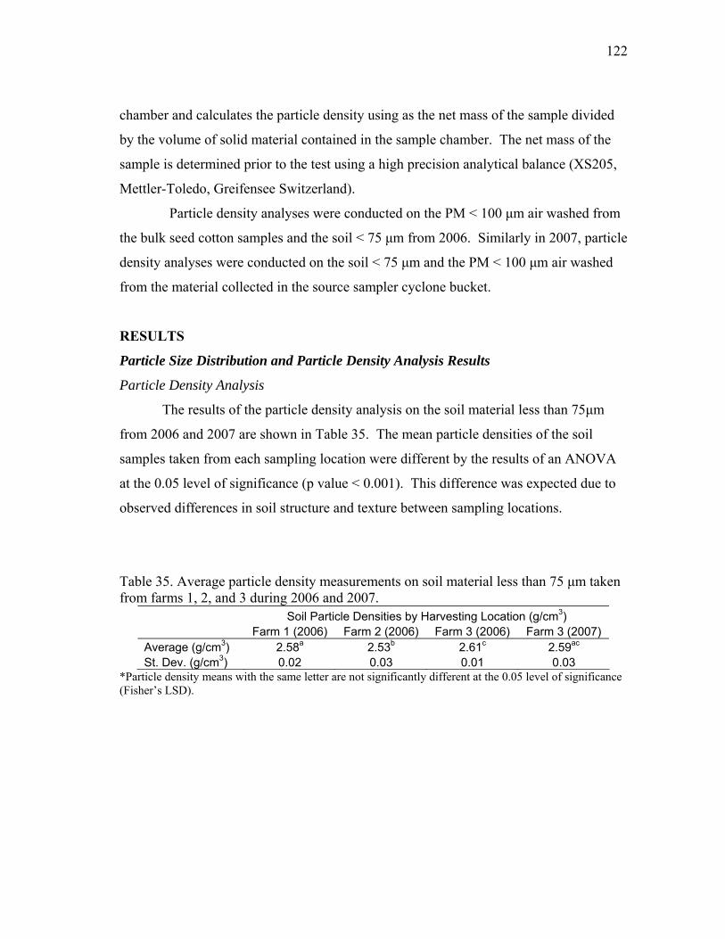
122
chamber and calculates the particle density using as the net mass of the sample divided
by the volume of solid material contained in the sample chamber. The net mass of the
sample is determined prior to the test using a high precision analytical balance (XS205,
Mettler-Toledo, Greifensee Switzerland).
Particle density analyses were conducted on the PM < 100 μm air washed from
the bulk seed cotton samples and the soil < 75 μm from 2006. Similarly in 2007, particle
density analyses were conducted on the soil < 75 μm and the PM < 100 μm air washed
from the material collected in the source sampler cyclone bucket.
RESULTS
Particle Size Distribution and Particle Density Analysis Results
Particle Density Analysis
The results of the particle density analysis on the soil material less than 75μm
from 2006 and 2007 are shown in Table 35. The mean particle densities of the soil
samples taken from each sampling location were different by the results of an ANOVA
at the 0.05 level of significance (p value < 0.001). This difference was expected due to
observed differences in soil structure and texture between sampling locations.
Table 35. Average particle density measurements on soil material less than 75 μm taken from farms 1, 2, and 3 during 2006 and 2007.
Soil Particle Densities by Harvesting Location (g/cm3) Farm 1 (2006) Farm 2 (2006) Farm 3 (2006) Farm 3 (2007) Average (g/cm3) 2.58a 2.53b 2.61c 2.59ac St. Dev. (g/cm3) 0.02 0.03 0.01 0.03
*Particle density means with the same letter are not significantly different at the 0.05 level of significance (Fisher’s LSD).

123
The results of the particle density analysis on the PM from the air wash
procedure on the bulk seed cotton samples taken during 2006 are shown in Table 36.
The air wash PM was mixed thoroughly before performing the analysis to help decrease
the bias in the particle density measurements due to sampling.
Table 36. Particle density analysis results for particulate matter less than 100 μm air washed from seed cotton samples taken during 2006.
Air Wash PM Particle Density (g/cm3)
Farm 1 1.86 Farm 2 1.79 Farm 3 1.97
The particle density results of the air wash PM from the three locations follow
the same trend as the soil material particle density results. This trend is likely a
consequence of the influence of soil particles as the primary constituent in the air wash
material (Wanjura et al., 2006). The other primary constituent of the air wash PM is
organic matter from the crop biomass. The presence of organic matter particles in the air
wash material results in the decrease in particle density between the soil material and air
wash PM. Wanjura et al. (2006) indicated that as much as 79% of the material air
washed from seed cotton samples is comprised of by soil material with the remaining
21% made up by plant and organic material.
Particle density results on the PM <75 μm air washed from the material collected
in the source sampler cyclone bucket during 2007 are shown in Table 37. Particle
density results for the material captured in the source sample cyclone bucket from 2006
were not available due to insufficient sample sizes. The mean particle density of the
material captured in the cyclone bucket is 1.59 g/cm3. The particle density of the
material in the cyclone bucket is lower than that of the material air washed from the seed
cotton samples due to the increased mass of volatile plant material (i.e. lint fiber and
pulverized leaf material). The results of an ash analysis on the air washed material from

124
the cyclone bucket indicated that the average ash content of the samples was 25.4 % (see
Appendix E). Wanjura et al. (2006) indicated that the ash content of a sample increases
with increasing amounts of soil material and reported average ash content for soil
material, PM <100 μm air washed from seed cotton, and ground plant material <75 μm
on the order of 94%, 80%, and 37% respectively.
Table 37. Particle density results of PM <100 μm air washed from material captured in the bucket of the source sampler cyclone during 2007.
Test
Particle Density (g/cm3)
1 1.62 2 1.60 3 1.60 4 1.59 5 1.57 6 1.56 7 1.56 8 1.57 9 1.61 10 1.63
Mean 1.59
St. Dev. 0.02
2006 Particle Size Distribution Analysis
PSD analyses were conducted on the PM from 10, 9, and 10 TSP filters from
farms 1, 2, and 3, respectively during 2006. Light PM loading resulted in the exclusion
of the other TSP filters. Typically, more than 200 μg of PM must be collected on a 47
mm diameter filter in order to conduct a PSD analysis. PSD analyses were conducted on
the source sampler filters (16 total filters, four per source sampling test) and the filters
containing the PM less than 100 μm from the material captured in the source sampler
cyclone bucket. The results of the PSD analyses from test 7 of farm 1, test 7 of farm 2,
and test 1 of farm 3 are shown in Figures 28, 29, and 30, respectively. The ESD MMD

125
and GSD of the best fit lognormal curves for the data shown in Figures 28, 29, and 30
are shown in Table 38.
Figure 28. Percent volume vs. ESD particle diameter PSDs for the air wash PM <100 μm (Air Wash Material), PM on the TSP sampler filter (Ambient TSP Sampler Filter), soil material < 75 μm (Soil Material), source sampler cyclone bucket material <100 μm (SS Cyclone Bucket Material), and PM on the source sampler filters (Source Sampler Filter)
from test 7 on farm 1 during 2006.

126
Figure 29. Percent volume vs. ESD particle diameter PSDs for the air wash PM <100 μm (Air Wash Material), PM on the TSP sampler filter (Ambient TSP Sampler Filter), soil material < 75 μm (Soil Material), source sampler cyclone bucket material <100 μm (SS Cyclone Bucket Material), and PM on the source sampler filters (Source Sampler Filter)
from test 7 on farm 2 during 2006.
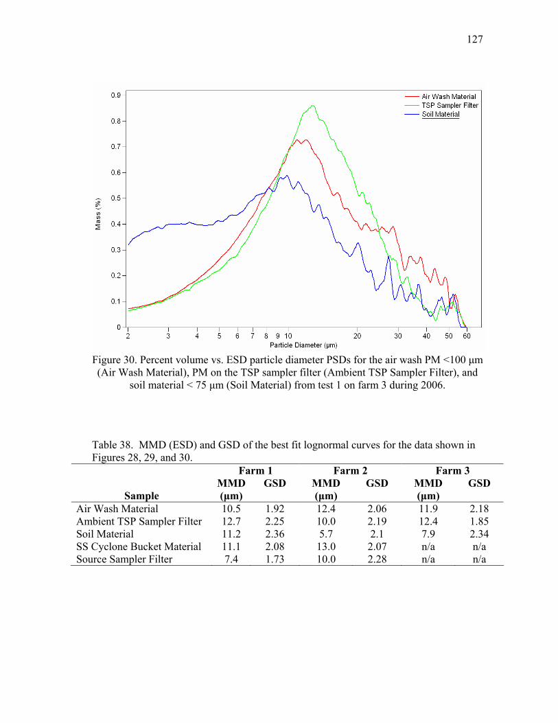
127
Figure 30. Percent volume vs. ESD particle diameter PSDs for the air wash PM <100 μm (Air Wash Material), PM on the TSP sampler filter (Ambient TSP Sampler Filter), and
soil material < 75 μm (Soil Material) from test 1 on farm 3 during 2006.
Table 38. MMD (ESD) and GSD of the best fit lognormal curves for the data shown in Figures 28, 29, and 30.
Farm 1 Farm 2 Farm 3 MMD GSD MMD GSD MMD GSD
Sample (μm) (μm) (μm) Air Wash Material 10.5 1.92 12.4 2.06 11.9 2.18 Ambient TSP Sampler Filter 12.7 2.25 10.0 2.19 12.4 1.85 Soil Material 11.2 2.36 5.7 2.1 7.9 2.34 SS Cyclone Bucket Material 11.1 2.08 13.0 2.07 n/a n/a Source Sampler Filter 7.4 1.73 10.0 2.28 n/a n/a
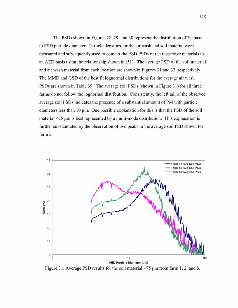
128
The PSDs shown in Figures 28, 29, and 30 represent the distribution of % mass
to ESD particle diameter. Particle densities for the air wash and soil material were
measured and subsequently used to convert the ESD PSDs of the respective materials to
an AED basis using the relationship shown in (51). The average PSD of the soil material
and air wash material from each location are shown in Figures 31 and 32, respectively.
The MMD and GSD of the best fit lognormal distributions for the average air wash
PSDs are shown in Table 39. The average soil PSDs (shown in Figure 31) for all three
farms do not follow the lognormal distribution. Consistently, the left tail of the observed
average soil PSDs indicates the presence of a substantial amount of PM with particle
diameters less than 10 μm. One possible explanation for this is that the PSD of the soil
material <75 μm is best represented by a multi-mode distribution. This explanation is
further substantiated by the observation of two peaks in the average soil PSD shown for
farm 2.
0
0.1
0.2
0.3
0.4
0.5
0.6
0.7
1 10 100
AED Particle Diameter (μm)
Mas
s (%
)
Farm #1 Avg Soil PSDFarm #2 Avg Soil PSDFarm #3 Avg Soil PSD
Figure 31. Average PSD results for the soil material <75 μm from farm 1, 2, and 3.

129
0
0.1
0.2
0.3
0.4
0.5
0.6
0.7
0.8
0.9
1 10 100
AED Particle Diameter (μm)
Mas
s (%
)Farm #1 Avg Air Wash PSD
Farm #2 Avg Air Wash PSD
Farm #3 Avg Air Wash PSD
Figure 32. Average PSD results of the air wash material from farm 1, 2, and 3.
Table 39. MMD and GSD values for the best fit lognormal distributions for the average air wash PSDs from farm 1, 2, 3.
Farm 1 Farm 2 Farm 3 MMD 14.6 15.3 16.4 GSD 2.00 2.05 2.00
130
The PSD of the air wash material from farm 1 and farm 2 falls between the PSDs
of the PM on the source sampler filters and source sampler cyclone bucket material.
This result is indicative of the separation of particles that takes place in the source
sampling system. PM similar to the air wash material is collected by the source
sampling probe and is fed into the barrel cyclone where larger particles are removed
from the air stream and accumulated in the cyclone bucket. The PSD of the PM
remaining in the sampler air stream (which is deposited on the filters) is then shifted to
the left of the PSD of the inlet material.
In order to determine the total mass fraction of a certain size PM sampled by the
source sampling system, the PSDs of the PM on the source sampler filters and the
cyclone bucket must be considered. Thus, a composite PSD was created for each source
sampling test by combining the filter and cyclone bucket PSDs on a mass weighted
average basis. The composite PSD matched the PSD of the air wash material more
closely than the soil material PSD. Thus, the composite PSD was converted from ESD
to AED using the particle density of the air wash material measured for the location of
the test. The composite PSDs of the source sampling tests are shown in Figure 33.
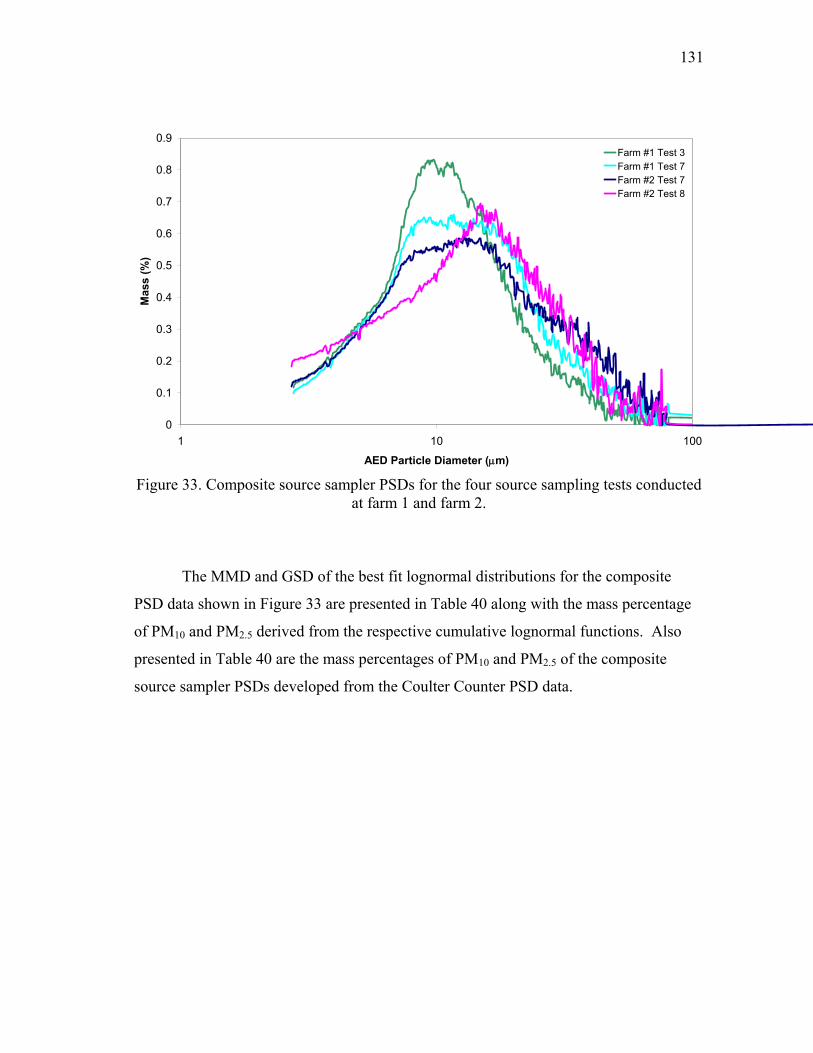
131
0
0.1
0.2
0.3
0.4
0.5
0.6
0.7
0.8
0.9
1 10 100
AED Particle Diameter (μm)
Mas
s (%
)Farm #1 Test 3Farm #1 Test 7Farm #2 Test 7Farm #2 Test 8
Figure 33. Composite source sampler PSDs for the four source sampling tests conducted
at farm 1 and farm 2.
The MMD and GSD of the best fit lognormal distributions for the composite
PSD data shown in Figure 33 are presented in Table 40 along with the mass percentage
of PM10 and PM2.5 derived from the respective cumulative lognormal functions. Also
presented in Table 40 are the mass percentages of PM10 and PM2.5 of the composite
source sampler PSDs developed from the Coulter Counter PSD data.
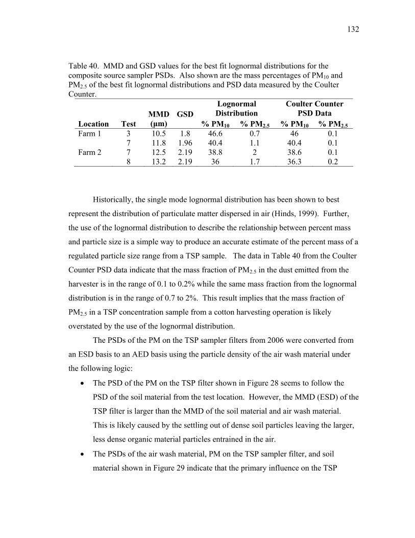
132
Table 40. MMD and GSD values for the best fit lognormal distributions for the composite source sampler PSDs. Also shown are the mass percentages of PM10 and PM2.5 of the best fit lognormal distributions and PSD data measured by the Coulter Counter.
Lognormal Distribution
Coulter Counter PSD Data
Location Test MMD(μm)
GSD % PM10 % PM2.5 % PM10 % PM2.5
Farm 1 3 10.5 1.8 46.6 0.7 46 0.1 7 11.8 1.96 40.4 1.1 40.4 0.1 Farm 2 7 12.5 2.19 38.8 2 38.6 0.1 8 13.2 2.19 36 1.7 36.3 0.2
Historically, the single mode lognormal distribution has been shown to best
represent the distribution of particulate matter dispersed in air (Hinds, 1999). Further,
the use of the lognormal distribution to describe the relationship between percent mass
and particle size is a simple way to produce an accurate estimate of the percent mass of a
regulated particle size range from a TSP sample. The data in Table 40 from the Coulter
Counter PSD data indicate that the mass fraction of PM2.5 in the dust emitted from the
harvester is in the range of 0.1 to 0.2% while the same mass fraction from the lognormal
distribution is in the range of 0.7 to 2%. This result implies that the mass fraction of
PM2.5 in a TSP concentration sample from a cotton harvesting operation is likely
overstated by the use of the lognormal distribution.
The PSDs of the PM on the TSP sampler filters from 2006 were converted from
an ESD basis to an AED basis using the particle density of the air wash material under
the following logic:
• The PSD of the PM on the TSP filter shown in Figure 28 seems to follow the
PSD of the soil material from the test location. However, the MMD (ESD) of the
TSP filter is larger than the MMD of the soil material and air wash material.
This is likely caused by the settling out of dense soil particles leaving the larger,
less dense organic material particles entrained in the air.
• The PSDs of the air wash material, PM on the TSP sampler filter, and soil
material shown in Figure 29 indicate that the primary influence on the TSP
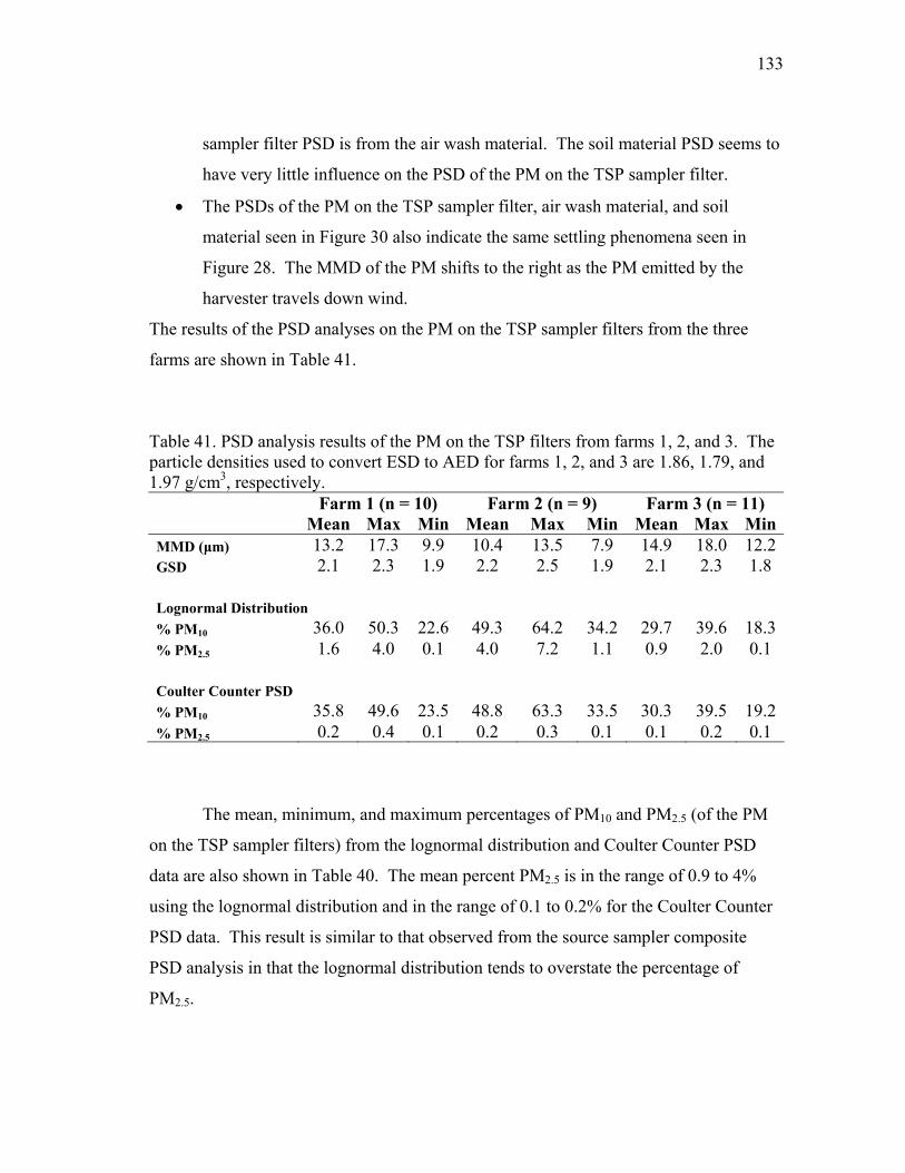
133
sampler filter PSD is from the air wash material. The soil material PSD seems to
have very little influence on the PSD of the PM on the TSP sampler filter.
• The PSDs of the PM on the TSP sampler filter, air wash material, and soil
material seen in Figure 30 also indicate the same settling phenomena seen in
Figure 28. The MMD of the PM shifts to the right as the PM emitted by the
harvester travels down wind.
The results of the PSD analyses on the PM on the TSP sampler filters from the three
farms are shown in Table 41.
Table 41. PSD analysis results of the PM on the TSP filters from farms 1, 2, and 3. The particle densities used to convert ESD to AED for farms 1, 2, and 3 are 1.86, 1.79, and 1.97 g/cm3, respectively. Farm 1 (n = 10) Farm 2 (n = 9) Farm 3 (n = 11) Mean Max Min Mean Max Min Mean Max MinMMD (μm) 13.2 17.3 9.9 10.4 13.5 7.9 14.9 18.0 12.2GSD 2.1 2.3 1.9 2.2 2.5 1.9 2.1 2.3 1.8 Lognormal Distribution % PM10 36.0 50.3 22.6 49.3 64.2 34.2 29.7 39.6 18.3% PM2.5 1.6 4.0 0.1 4.0 7.2 1.1 0.9 2.0 0.1 Coulter Counter PSD % PM10 35.8 49.6 23.5 48.8 63.3 33.5 30.3 39.5 19.2% PM2.5 0.2 0.4 0.1 0.2 0.3 0.1 0.1 0.2 0.1
The mean, minimum, and maximum percentages of PM10 and PM2.5 (of the PM
on the TSP sampler filters) from the lognormal distribution and Coulter Counter PSD
data are also shown in Table 40. The mean percent PM2.5 is in the range of 0.9 to 4%
using the lognormal distribution and in the range of 0.1 to 0.2% for the Coulter Counter
PSD data. This result is similar to that observed from the source sampler composite
PSD analysis in that the lognormal distribution tends to overstate the percentage of
PM2.5.

134
2007 Particle Size Distribution Analysis
The TSP samplers used to measure concentrations during 2007 yielded 26 filters
with sufficient mass for PSD analysis. The particle density of the material air washed
from the source sampler cyclone bucket was used to convert the PSD results on the TSP
filters from an ESD to AED basis. The upper tail of the distributions for most of the
filters exhibited the spread pattern shown by the PSD in Figure 34. The TSP filter PSD
shown in Figure 34 was taken from test 20 at farm 1 during 2007. Also shown in Figure
34 is the overall average lognormal PSD of the TSP filters used in the PSD analysis from
2007 (MMD = 14.7 μm, GSD = 2.23). The statistics of the TSP filter PSD analysis are
shown in Table 42.
Table 42. TSP sampler filter PSD analysis result statistics for samples taken on farm 3 during 2007. The particle density used to convert ESD to AED was 1.59 g/cm3.
TSP Sampler PSD Statistics Mean Max Min MMD 14.7 21.1 9.7 GSD 2.2 2.5 2.0 Lognormal Distribution % PM10 33.6 52.0 16.0 % PM2.5 1.7 4.3 0.2 Coulter Counter PSD % PM10 34.7 50.9 21.7 % PM2.5 0.1 0.2 0.0

135
0
0.1
0.2
0.3
0.4
0.5
0.6
0.7
0.8
1 10 100
Aerodynamic Particle Diameter (μm)
% M
ass
TSP Filter PSD2007 Average Lognormal PSD
Figure 34. PSD of a downwind TSP sampler from test 20 at farm 3 during 2007 shown with the farm average lognormal PSD of the TSP sampler filters (MMD = 14.7, GSD =
2.23).
The 2007 PSD results of the soil material <75 μm agree well with those observed
during 2006. The average soil PSD (see Figure 35) exhibits a left skew with a
significant mass of particles with AED less than 10 μm. The mean MMD and GSD of
the soil material PSDs are 16.3 and 2.4, respectively. The average statistics of the soil
material PSD analyses is shown in Table 43.
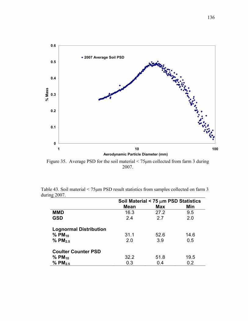
136
0
0.1
0.2
0.3
0.4
0.5
0.6
1 10 100Aerodynamic Particle Diameter (mm)
% M
ass
2007 Average Soil PSD
Figure 35. Average PSD for the soil material < 75μm collected from farm 3 during
2007.
Table 43. Soil material < 75μm PSD result statistics from samples collected on farm 3 during 2007.
Soil Material < 75 μm PSD Statistics Mean Max Min MMD 16.3 27.2 9.5 GSD 2.4 2.7 2.0 Lognormal Distribution % PM10 31.1 52.6 14.6 % PM2.5 2.0 3.9 0.5 Coulter Counter PSD % PM10 32.2 51.8 19.5 % PM2.5 0.3 0.4 0.2
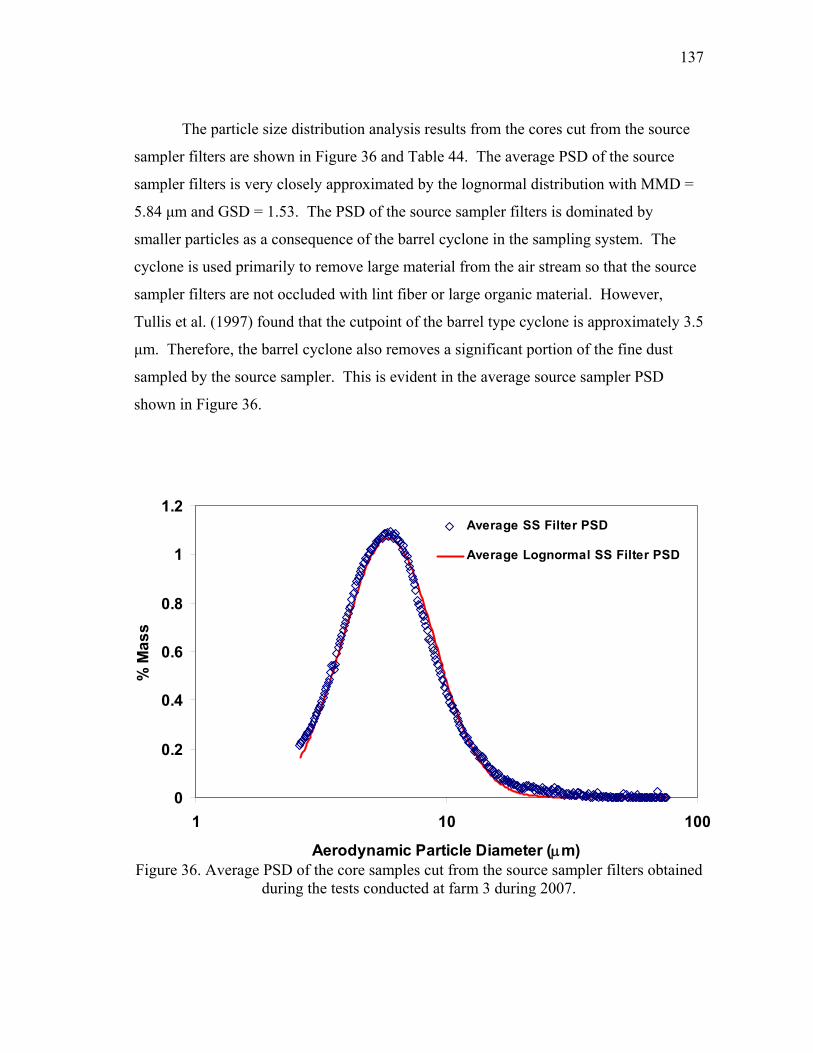
137
The particle size distribution analysis results from the cores cut from the source
sampler filters are shown in Figure 36 and Table 44. The average PSD of the source
sampler filters is very closely approximated by the lognormal distribution with MMD =
5.84 μm and GSD = 1.53. The PSD of the source sampler filters is dominated by
smaller particles as a consequence of the barrel cyclone in the sampling system. The
cyclone is used primarily to remove large material from the air stream so that the source
sampler filters are not occluded with lint fiber or large organic material. However,
Tullis et al. (1997) found that the cutpoint of the barrel type cyclone is approximately 3.5
μm. Therefore, the barrel cyclone also removes a significant portion of the fine dust
sampled by the source sampler. This is evident in the average source sampler PSD
shown in Figure 36.
0
0.2
0.4
0.6
0.8
1
1.2
1 10 100
Aerodynamic Particle Diameter (μm)
% M
ass
Average SS Filter PSD
Average Lognormal SS Filter PSD
Figure 36. Average PSD of the core samples cut from the source sampler filters obtained
during the tests conducted at farm 3 during 2007.

138
Table 44. PSD analysis result statistics for the source sampler filters collected during the tests conducted on farm 3 during 2007.
Source Sampler Filter PSD Statistics Mean Max Min MMD 5.8 6.7 5.4 GSD 1.5 1.6 1.5 Lognormal Distribution % PM10 89.8 94.6 79.2 % PM2.5 2.3 4.4 1.3 Coulter Counter PSD % PM10 87.6 92.9 77.0 % PM2.5 0.2 0.3 0.1
The results of the PSD analysis on the PM < 100 μm air washed from the
material captured in the source sampler cyclone bucket are shown in Figure 37 and
Table 45. The lognormal approximation of the measured PSD is a fair approximation
although it does not seem to match as well as the source sampler filter data. One
possible reason for this is the increased presence of small lint fiber and pulverized leaf
material.
Table 45. PSD results for the PM < 100 μm air washed from the material captured in the source sampler cyclone bucket from the tests conducted on farm 3 during 2007.
Source Sampler Cyclone Bucket
PM < 100 μm PSD Statistics Mean Max Min MMD 16.6 18.8 14.7 GSD 2.0 2.2 1.9 Lognormal Distribution % PM10 24.1 29.3 19.4 % PM2.5 0.4 0.7 0.2 Coulter Counter PSD % PM10 25.3 29.8 21.4 % PM2.5 0.0 0.0 0.0
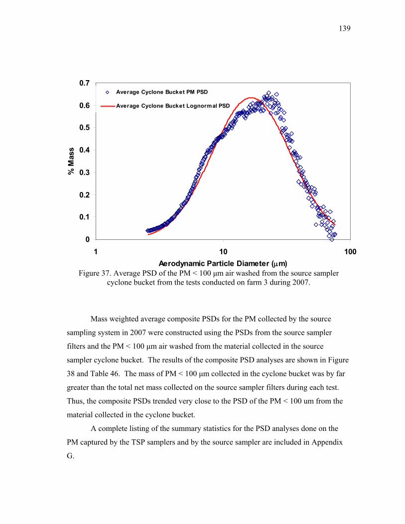
139
0
0.1
0.2
0.3
0.4
0.5
0.6
0.7
1 10 100Aerodynamic Particle Diameter (μm)
% M
ass
Average Cyclone Bucket PM PSD
Average Cyclone Bucket Lognormal PSD
Figure 37. Average PSD of the PM < 100 μm air washed from the source sampler
cyclone bucket from the tests conducted on farm 3 during 2007.
Mass weighted average composite PSDs for the PM collected by the source
sampling system in 2007 were constructed using the PSDs from the source sampler
filters and the PM < 100 μm air washed from the material collected in the source
sampler cyclone bucket. The results of the composite PSD analyses are shown in Figure
38 and Table 46. The mass of PM < 100 μm collected in the cyclone bucket was by far
greater than the total net mass collected on the source sampler filters during each test.
Thus, the composite PSDs trended very close to the PSD of the PM < 100 um from the
material collected in the cyclone bucket.
A complete listing of the summary statistics for the PSD analyses done on the
PM captured by the TSP samplers and by the source sampler are included in Appendix
G.

140
0
0.2
0.4
0.6
0.8
1
1.2
1 10 100
Aerodynamic Particle Diameter
% M
ass
Average SS Filter PSD
Average SS Cyclone Bucket PSD
Average SS Composite PSD
Figure 38. Average PSDs for the source sampler filters, PM < 100 μm captured in the source sampler cyclone bucket, and the mass weighted average composite PSD for the tests conducted on farm 3 during 2007.

141
Table 46. Result statistics for the mass weighted average composite PSDs developed from the PSDs of the source sampler filters and PM < 100 μm captured in the source sampler cyclone bucket during 2007.
Source Sampler Composite PSD
Statistics Mean Max Min MMD 14.3 16.6 13.4 GSD 2.2 2.4 2.1 Lognormal Distribution % PM10 32.7 35.5 27.3 % PM2.5 1.40 2.44 0.84 Coulter Counter PSD % PM10 34.0 36.6 29.5 % PM2.5 0.06 0.07 0.05
142
CHAPTER VI
SUMMARY AND CONCLUSIONS
Cotton producers in some states across the US cotton belt are facing increased
regulatory pressure from state air pollution regulatory agencies through the air quality
permitting process. Historically, producers of agricultural crops have been exempt from
air pollution permitting requirements. Today this is not the case. Growers in California
and Arizona are required to obtain air quality permits from state regulators for each crop
they plant, including cotton. These permits are granted to the producer once they have
submitted management practice plans which detail the steps that the producer will use to
help reduce fugitive emissions from their operation.
Poor regional air quality in these areas forced regulators to focus in on sources,
identified through annual emissions inventories, which significantly contribute to the
ambient concentration of regulated sizes of PM. Through this process, cotton production
was identified as a significant source of PM10 in the San Joaquin Valley of California. A
likely cause for the identification of cotton production as a significant source of PM10 is
the inaccurate emission factor used to calculate the annual PM10 emissions inventory for
the region.
Emission factors are estimates of the amount of a specific pollutant emitted by an
operation on a unit of production basis (e.g. kg PM10/ha or kg PM10/bale). Emission
factors are used by air pollution regulators to calculate emissions inventories and as the
basis for emission rates used in dispersion modeling to predict downwind concentrations
from a source. Accurate emission factors are essential to the regulatory process for the
appropriate regulation of industrial and agricultural sources and for the protection of
human health and wellbeing.
Little accurate emission factor data is available for PM emissions generated by
agricultural field operations including cotton harvesting. The objective of this work was
to develop an accurate, science based, PM emission factor for cotton harvesting in terms
of TSP, PM10, and PM2.5.
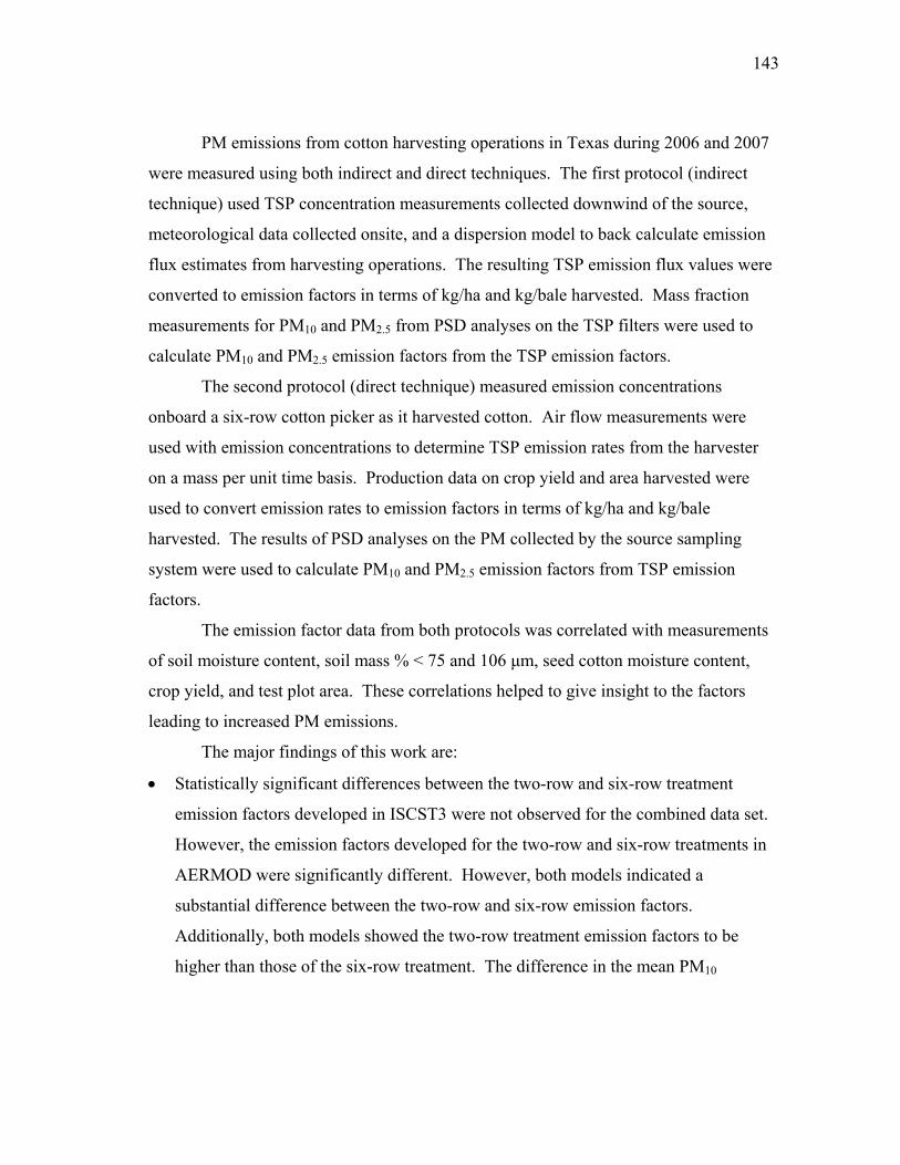
143
PM emissions from cotton harvesting operations in Texas during 2006 and 2007
were measured using both indirect and direct techniques. The first protocol (indirect
technique) used TSP concentration measurements collected downwind of the source,
meteorological data collected onsite, and a dispersion model to back calculate emission
flux estimates from harvesting operations. The resulting TSP emission flux values were
converted to emission factors in terms of kg/ha and kg/bale harvested. Mass fraction
measurements for PM10 and PM2.5 from PSD analyses on the TSP filters were used to
calculate PM10 and PM2.5 emission factors from the TSP emission factors.
The second protocol (direct technique) measured emission concentrations
onboard a six-row cotton picker as it harvested cotton. Air flow measurements were
used with emission concentrations to determine TSP emission rates from the harvester
on a mass per unit time basis. Production data on crop yield and area harvested were
used to convert emission rates to emission factors in terms of kg/ha and kg/bale
harvested. The results of PSD analyses on the PM collected by the source sampling
system were used to calculate PM10 and PM2.5 emission factors from TSP emission
factors.
The emission factor data from both protocols was correlated with measurements
of soil moisture content, soil mass % < 75 and 106 μm, seed cotton moisture content,
crop yield, and test plot area. These correlations helped to give insight to the factors
leading to increased PM emissions.
The major findings of this work are:
• Statistically significant differences between the two-row and six-row treatment
emission factors developed in ISCST3 were not observed for the combined data set.
However, the emission factors developed for the two-row and six-row treatments in
AERMOD were significantly different. However, both models indicated a
substantial difference between the two-row and six-row emission factors.
Additionally, both models showed the two-row treatment emission factors to be
higher than those of the six-row treatment. The difference in the mean PM10
144
emission factors for the two-row and six-row treatments developed in ISCST3 and
AERMOD were 1.08 and 3.61 kg/ha, respectively.
• Source measurement of emissions onboard the six-row cotton picker were
successfully conducted during 2006 and 2007. The emission factors developed with
the source sampling protocol are the most accurate emission factors ever developed
for cotton harvesting. Furthermore, the emission factors developed through the
source measurement protocol are recommended for regulatory use due to the low
uncertainty and high precision of the measurements. The TSP, PM10, and PM2.5
emission factors from the source measurements conducted during 2007 were 1.64 ±
0.37, 0.55 ± 0.12, and 1.58E-03 ± 4.5E-04 kg/ha, respectively (1.46 ± 0.33, 0.49 ±
0.11, and 1.41E-03 ± 4.01E-04 lb/ac, respectively). These emission factors are
inclusive of the emission factors for the PM generated by the interaction of the
harvester wheels and the soil surface as the machine moves through the field. The
PM generated by the wheels of the harvester account for approximately 15% of the
total emission factor.
• Additional analysis of the emission rates calculated from the source emission
concentration measurements indicates that PM emissions from cotton harvesting
operations are more closely correlated with crop yield than with land area harvested.
Thus, the most appropriate basis on which to report emission factors from cotton
harvesting is in terms of mass per lint bale harvested (e.g. kg/bale). In terms of
kg/bale, the TSP, PM10, and PM2.5 emission factors from the source measurements of
PM emissions from the six row machine were 0.22 ± 0.019, 0.07 ± 0.007, and 2.15E-
4 ± 1.49E-5 kg/bale, respectively (0.48 ± 0.04, 0.15 ± 0.015, and 4.74E-4 ± 3.3E-5
lb/bale, respectively). These emission factors are inclusive of the PM emissions
generated by the harvester wheel/soil surface interaction and represent the average
mass per bale emission factors measured over a crop yield range from 5.9 to 9.3
bales/ha (2.4 to 3.8 bales/ac).
• Particle size distribution analysis of the TSP sampler filters indicates that the PSD of
the dust measured downwind of the harvesting operation can be approximated by a

145
lognormal density function characterized by MMD and GSD values of 14 μm and
2.2 respectively. The mass percent PM10 and PM2.5 from PSD analysis of the TSP
filters were on the order of 35 and 0.1%, respectively. These results are further
corroborated by the PSD analysis on the PM captured on the source sampler filters
and PM < 100 μm captured in the source sampler cyclone bucket.
FUTURE WORK
The emission factors resulting from this work were developed with state-of-the-
art methods in order to produce accurate, science based PM emissions data from cotton
harvesting. However, additional work is needed to better quantify the uncertainty in the
emission factors developed through the dispersion modeling process. As AERMOD is
incorporated into the regulatory program of each state, it is imperative that appropriate
emission factors are used to predict downwind source impacts. It is likely the case that
most states will use emission factors in AERMOD which were previously used in
ISCST3. This scenario will be problematic from a regulatory standpoint.
The following have been identified for future work in this area:
1. Quantification of the variability in emission factors developed in ISCST3 and
AERMOD due to variability in wind speed and direction. While traditional first
order sensitivity analysis on ISCST3 and AERMOD may be problematic, a
Monte Carlo simulation model may be used to generate meteorological data files
containing several thousand lines of data from wind speed and wind direction
distributions. These files could then be used to develop emission factors for
several different receptor locations within ISCST3 or AERMOD. Additional
variations on this might include different source to receptor configurations.
2. Compare the emission factor results from AERMOD using meteorological data
prepared through the AERMET preprocessor and meteorological data prepared
using the procedures described in this work.
3. Begin the process of obtaining adoption of the emission factors developed in this
work at the state and national regulatory levels.

146
REFERENCES
Beckman Coulter. 2002. Beckman Coulter Multisizer 3 – Operator’s Manual. PN 8321681 rev. B. Fullerton, CA.: Beckman Coulter, Inc.
Beychok, M.R. 1994. Fundamentals of Stack Gas Dispersion. 3rd ed. Newport Beach,
CA: Milton R. Beychok. Buser, M. D., C.B. Parnell, R. E. Lacey, B.W. Shaw, and B.W. Auvermann. 2001.
Inherent biases of PM10 and PM2.5 samplers based on the interaction of particle size and sampler performance characteristics. ASAE Paper No. 011167. St. Joseph, MI.: ASAE.
Buser, M.D. 2004. Errors associated with particulate matter measurements on rural
sources: Appropriate basis for regulating cotton gins. Unpublished Ph.D. diss. College Station, TX.: Texas A&M University, Department of Biological and Agricultural Engineering.
California Air Resources Board (CARB). 2003. Senate Bill 700 - Florez. Sacramento,
CA: California Air Resources Board. Available at, http://www.arb.ca.gov/ag/sb700/sb700.pdf. Accessed 12/15/2006.
Capareda, S.C., C.B. Parnell, B.W. Shaw, and J.D. Wanjura. 2005. Particle size
distribution analysis of cotton gin dust and its impact on PM10 concentration measurements. In Proc. of the 2005 Beltwide Cotton Conferences, CD-Rom. New Orleans, LA.: National Cotton Council.
Code of Federal Regulations (CFR). 1996. Requirements for preparation, adoption, and
submittal of implementation plans, Subpart I: Review of new sources and modifications. 40CFR, Part 51.160: Office of the Federal Register, National Archives, and Records Administration. Washington DC: U.S. Government Printing Office.
Code of Federal Regulations (CFR). 1999. Method 5: Determination of particulate
matter emissions from stationary sources. 40CFR, Part 60: Appendix A-3. Office of the Federal Register, National Archives, and Records Administration. Washington D.C.: U.S. Government Printing Office.

147
Code of Federal Regulations (CFR). 2007. Determination of particulate matter emissions from stationary sources. 40CFR, Part 60: Appendix A. Office of the Federal Register, National Archives, and Records Administration. Washington D.C.: U.S. Government Printing Office.
Environmental Protection Agency (EPA). 1995a. Compilation of air pollutant emission
factors (AP-42). Research Triangle Park, NC: EPA. Environmental Protection Agency (EPA). 1995b. User’s guide for the industrial source
complex dispersion models – Volume II: description of model algorithms. EPA-454/B-95-003b. Office of Air Quality Planning and Standards - Emissions Monitoring and Analysis Division. Research Triangle Park, NC. USEPA.
Environmental Protection Agency (EPA). 2000. Meteorological monitoring guidelines
for regulatory modeling applications. EPA-454/R-99-005. Research Triangle Park, NC.: US Environmental Protection Agency, Office of Air Quality Planning and Standards Emission Factors and Inventory Group.
Environmental Protection Agency (EPA). 2004. AERMOD: Description of model
formulation. EPA-454/R-03-004. Office of Air Quality Planning and Standards - Emissions Monitoring and Analysis Division. Research Triangle Park, NC. USEPA.
Environmental Protection Agency (EPA). 2006. Fact sheet: Final revisions to the
national ambient air quality standards for particle pollution (Particulate Matter). Research Triangle Park, NC.: US Environmental Protection Agency. Available at, http://epa.gov/pm/actions.html. Accessed 12/15/2006.
Etling, D. 1996. Temporal and spatial variations in the ABL. In Modeling of
Atmospheric Flow Fields, 21 – 41. River Edge, NJ: World Scientific Publishing Company.
Faulkner, W.B. and B.W. Shaw. 2006. Efficiency and pressure drop of cyclones across a
range of inlet velocities. Applied Engineering in Agriculture 22(1): 155-161. Federal Register. 2005. Revision to the guideline on air quality models: Adoption of a
preferred general purpose (Flat and Complex Terrain) dispersion model and other revisions; Final rule. Federal Register 70:68218-3.

148
Federal Register. 2006. National ambient air quality standards for particulate matter; Final rule. 40 CFR Part 50. Federal Register 71 (200): 61144. Office of the Federal Register, National Archives, and Records Administration. Washington DC: U.S. Government Printing Office.
Flocchini, R.G., et al. 2001. Sources and sinks of PM10 in the San Joaquin valley, final
report. United States Department of Agriculture – Special Research Grants Program. Contract Nos. 94-33825-0383 and 98-38825-6063. Davis, CA: University of California at Davis.
Garratt, J.R. 1992. The Atmospheric Boundary Layer. New York, N.Y. Cambridge
University Press. Goodrich, L.B. 2006. A PM10 emission factor for free stall dairies. MS thesis. College
Station, TX.: Department of Biological and Agricultural Engineering, Texas A&M University.
Hinds, W. C. 1999. Aerosol Technology: Properties, Behavior, and Measurement of
Airborne Particles. 2nd ed. New York, N.Y.: John Wiley & Sons, Inc. Hiscox, A.L., D.R. Miller, C.J. Nappo, and J. Ross. 2006. Dispersion of fine spray from
aerial applications in stable atmospheric conditions. Trans. ASAE 49(5): 1513-1520.
Johnson, R.A. and D.W. Wichern. 2002. Applied Multivariate Statistical Analysis. 5th
ed. Upper Saddle River, N.J.: Prentice-Hall, Inc. Kaimal, J.C., Finnigan, J.J. 1994. Atmospheric Boundary Layer Flows: Their Structure
Measurement. New York, N.Y.: Oxford University Press. Kline, S.J., and F.A. McClintock. 1953. Describing uncertainties in single sample
experiments. Mechanical Engineering 75:3-8. Manwell, J.F., J.G. McGowan, and A.L. Rogers. 2002. Wind Energy Explained –
Theory, Design, and Application, 44 - 45. West Sussex, England: John Wiley & Sons. Ltd.
McFarland, A. R. and C. A. Ortiz. 1983. Evaluation of prototype PM-10 inlets with
cyclonic fractionators. Paper No. 33.5 presented at, The 76th Annual Meeting and Exposition of the Air Pollution Control Association. Atlanta, GA.
149
Mihalski, K.D. 1996. The design of a pre-collector for cyclone separators. MS thesis.
College Station, TX.: Department of Biological and Agricultural Engineering, Texas A&M University.
Parnell, S. 1994. Dispersion modeling for prediction of emission factors for cattle
feedyards. MS thesis. College Station, TX.: Department of Agricultural Engineering, Texas A&M University.
Reynolds, O. 1895. On the dynamical theory of incompressible viscous fluids and the
determination of the criterion. Philos. Transactions of the Royal Society of London 186A, 123 – 164.
San Joaquin Valley Air Pollution Control District (SJVAPCD). 2004a. Rule 4550 –
Conservation Management Practices. Modesto, CA.: SJVAPCD. San Joaquin Valley Air Pollution Control District (SJVAPCD). 2004b. List of
Conservation Management Practices. Modesto, CA.: SJVAPCD. Snyder, J.W., T.R. Blackwood. 1977. Source assessment: Mechanical harvesting of
cotton – state of the art. EPA-600/2-77-107d. Cincinnati, OH: United States Environmental Protection Agency.
Stull, R.B. 1988. An Introduction to Boundary Layer Meteorology. Boston, MA.:
Kluwer Academic Publishers. Texas Commission on Environmental Quality (TCEQ). 2005. AERMOD Training.
available on the web at: http://www.tceq.state.tx.us/files/aermet.pdf_4012036.pdf. Accessed 11/25/2007.
Texas Commission on Environmental Quality (TCEQ). 2007. One year meteorological
data file for Burleson Co. available on the web at: ftp://ftp.tceq.state.tx.us/pub/OPRR/APD/AERMET/AERMETv04300/AERMETDataSetsByCounty/. Accessed 11/25/2007.
Trinity Consultants. 2007. BREEZE MetView v6.0.7 – User’s Manual. Dallas, TX.:
Trinity Consultants.
150
Tullis, A.W., B.W. Shaw, C.B. Parnell, P.P. Buharivala, M.A. Demny, and S.S. Flannigan. 1997. Design and analysis of the barrel cyclone. In Proc. Beltwide Cotton Conference, 2:1520-1525. Memphis, TN.: National Cotton Council.
USDA. 1972. Standard Procedures for Foreign Matter and Moisture Analytical Tests
Used in Cotton Ginning Research. Agriculture Handbook No. 422. US Government Printing Office: 1972 O-443-789.
USDA. 2007. Cotton Production in the US: 1977 – 2007. National Agricultural Statistics
Database. Washington, DC.: USDA National Agricultural Statistics Service. Available at, http://www.nass.usda.gov/QuickStats/. Accessed 25 November, 2007.
Van Boxel, J.H., G. Sterk, and S.M. Arens. 2004. Sonic anemometers in aeolian
sediment transport research. Geomorphology 59: 131 – 147. Wanjura, J.D., C.B. Parnell, Jr., B.W. Shaw and R.E. Lacey. 2004. A protocol for
determining a fugitive dust emission factor from a ground level area source. ASAE Paper No. 044018. St. Joseph, MI: ASAE.
Wanjura, J.D., M.D. Buser, D.P. Whitelock, S.C. Capareda, C.B. Parnell, Jr., B.W.
Shaw, and R.E. Lacey. 2005a. A method of estimating FRM PM10 sampler performance characteristics using particle size analysis and collocated TSP and PM10 samplers. ASAE Paper No. 054015. St. Joseph, MI: ASAE.
Wanjura, J.D., C.B. Parnell, Jr., B.W. Shaw, and R.E. Lacey. 2005b. Design and
evaluation of a low volume total suspended particulate sampler. Trans. ASAE 48(4): 1547-1552.
Wanjura, J.D., M.D. Buser, C.B. Parnell, B.W. Shaw, and R.E. Lacey. 2005c. A
simulated approach to estimating PM10 and PM2.5 concentrations downwind from cotton gins. Trans. ASAE 48(5): 1919-1925.
Wanjura, J.D. 2005. Engineering approaches to address errors in measured and predicted
particulate matter concentrations. MS thesis. College Station, TX.: Department of Biological and Agricultural Engineering, Texas A&M University.
Wanjura, J.D., C.B. Parnell, Jr., B.W. Shaw, and S.C. Capareda. 2006. Particle size
distribution of PM emitted from cotton harvesting. ASABE Paper No. 064168. St. Joseph, MI.: ASABE.

151
Wanjura, J.D., B.W. Shaw, C.B. Parnell Jr., S.C. Capareda, and W.B. Faulkner. 2007. A preliminary particulate matter emission factor from cotton harvesting. In Proc. 2007 Beltwide Cotton Conferences, CD-Rom. Memphis, TN.: National Cotton Council.

152
APPENDIX A
SOIL SIEVING PROCEDURE
153
The following procedure was used to sieve the soil samples collected from farms
1, 2, and 3 during 2006 and 2007. The soil mass percent < 75 and 106 μm were
determined through this procedure.
Cleaning the Sieves:
How do you know if the sieve is clean?
You can determine if they are clean by weighing them and comparing their
current weight to the clean weight written on the side of the sieve. Be sure that the
current weight is within 0.01 g of the clean weight.
Cleaning the sieves:
The large opening sieves can be cleaned with a nylon bristle brush (paint brush)
and the small mesh sieves (opening size <#80) should be brushed off first before being
placed in the ultrasonic cleaner for 5 minutes. (The ultrasonic bath should be filled with
water so that the top of the water is about ½” above the top rim of the sieve.) After the
sieves come out of the ultrasonic bath, they must be dried thoroughly. Complete drying
of the small mesh sieves can be accomplished by placing them in a drying oven at 100°C
for 1 hour. After drying the sieves make sure that the current weight matches the clean
weight within 0.01g.
Sieve Analysis Procedure
Step 1:
Locate the following sieves and place in the indicated order with the largest
opening size on top:
Stack 1: 0.875”, 0.625”, 0.375”, 0.3125”, #10, Pan #1
Stack 2: #14, #25, #80, #140, #200, Pan #2
Place a lid on top of each stack before loading the two stacks into the shaker. Make sure
that the lids, pans, and sieves are clean before use.

154
Step 2:
Next weigh out approximately 500 – 700 g of material in a scale pan. Record the
total (gross) weight of the scale pan plus the material on the work sheet.
Step 3:
Pour the material from the scale pan into the top sieve of stack 1. Replace the lid
on the top sieve and install the large (black) sieve stack cover with the cork pointing up.
Lower the white hammer arm down onto the cork and set the timer on the shaker to 20
minutes.
Step 4:
Start the machine by pressing the start/resume button on the shaker and let the
shaker run for the set time.
Step 5:
Once the machine has finished shaking, remove the first stack of sieves and carry
them to the scale. Carefully weigh each sieve and the pan in the stack to the nearest
0.01g and record these weights on the work sheet under the gross weight column. Be
very careful not to loose any material out of the sieves or pan during the weighing
process.
Step 6:
After the sieves have been weighed, collect material samples from each sieve and
pan according to the details of the experiment design.
Step 7:
Pour the material from the pan in stack one into the top sieve in stack two and
replace the brass lid on top of stack 2.
155
Step 8:
Once the samples have been taken and the material in the pan transferred to the
second stack, empty and clean each sieve and pan with the nylon bristle brush. After
cleaning, weigh each sieve and pan and record the weight on the work sheet under the
tare column. Make sure that the tare weight is within 0.01g of the clean weight on the
side of the sieve.
Step 9:
Reload the first stack of sieves into the machine. Weigh out a new sample of
material to be placed in the top sieve of stack 1 as was done in step 2 – 3. Be sure to
record this new gross weigh of initial material mass on a new work sheet.
Step 10:
Repeat steps 3 – 6 for both stacks of sieves. At this point, be sure to record the
gross and tare weights of the second stack sieves on the first work sheet and the gross
and tare weights of the first stack sieves on the second work sheet. This is a semi-
continuous batch process where the machine always has two samples running at one
time.
Step 11:
When cleaning the second stack of sieves, brush them off first and check the
clean weights before cleaning them in the ultrasonic bath. Several samples may be able
to be run before cleaning the small mesh screens in the ultrasonic bath. Don’t run more
than 3 samples before cleaning the small mesh screens in the ultrasonic bath.
Once all of the samples have been processed for one day, clean the sieves
according to the previous instructions.

156
APPENDIX B
METEOROLOGICAL DATA DEVELOPED FOR USE IN AERMOD FROM 3D
SONIC ANEMOMETER MEASUREMENTS

157
Table B-1. Meteorological parameters measured and observed onsite during the tests conducted on farm 3 during 2007.
Test HR Wind Speed
Wind Direction
Wind Reference
Height Temp
Temperature Reference
Height Precipitation
Code Precipitation
Rate Relative Humidity
Station Pressure
Cloud Cover
m/s degrees m K m mm/hr % mb tenths 1 14 2.21 31 3.0 303.8 2.0 0 0.00 59 1010 0 1 15 2.31 35 3.0 304.0 2.0 0 0.00 59 1010 0
2 11 1.87 57 3.0 299.9 2.0 0 0.00 51 990 0
3 15 2.25 25 3.0 303.0 2.0 0 0.00 34 1008 1
4 16 1.82 27 3.0 303.3 2.0 0 0.00 32 1007 2
5 18 1.00 34 3.0 301.8 2.0 0 0.00 46 1006 1
6 15 1.70 132 3.0 303.3 2.0 0 0.00 32 1007 0 6 16 2.16 157 3.0 303.4 2.0 0 0.00 32 1007 0
7 18 1.44 128 3.0 297.9 2.0 0 0.00 48 1005 0 7 19 1.05 124 3.0 296.3 2.0 0 0.00 48 1005 0
8 11 5.47 183 3.0 299.6 2.0 0 0.00 46 1006 0 8 12 5.24 178 3.0 300.2 2.0 0 0.00 46 1006 0
9 13 4.91 171 3.0 302.3 2.0 0 0.00 31 1004 1 9 14 4.91 178 3.0 302.9 2.0 0 0.00 31 1004 1
10 15 5.34 165 3.0 303.5 2.0 0 0.00 30 1003 2
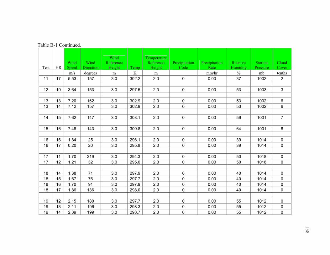
158
Table B-1 Continued.
Test HR Wind Speed
Wind Direction
Wind Reference
Height Temp
Temperature Reference
Height Precipitation
Code Precipitation
Rate Relative Humidity
Station Pressure
Cloud Cover
m/s degrees m K m mm/hr % mb tenths 11 17 5.53 157 3.0 302.2 2.0 0 0.00 37 1002 2
12 19 3.64 153 3.0 297.5 2.0 0 0.00 53 1003 3
13 13 7.20 162 3.0 302.9 2.0 0 0.00 53 1002 6 13 14 7.12 157 3.0 302.9 2.0 0 0.00 53 1002 6
14 15 7.62 147 3.0 303.1 2.0 0 0.00 56 1001 7
15 16 7.48 143 3.0 300.8 2.0 0 0.00 64 1001 8
16 16 1.84 25 3.0 296.1 2.0 0 0.00 39 1014 0 16 17 0.20 20 3.0 295.8 2.0 0 0.00 39 1014 0
17 11 1.70 219 3.0 294.3 2.0 0 0.00 50 1018 0 17 12 1.21 32 3.0 295.0 2.0 0 0.00 50 1018 0
18 14 1.38 71 3.0 297.9 2.0 0 0.00 40 1014 0 18 15 1.67 76 3.0 297.7 2.0 0 0.00 40 1014 0 18 16 1.70 91 3.0 297.9 2.0 0 0.00 40 1014 0 18 17 1.86 136 3.0 298.0 2.0 0 0.00 40 1014 0
19 12 2.15 180 3.0 297.7 2.0 0 0.00 55 1012 0 19 13 2.11 196 3.0 298.3 2.0 0 0.00 55 1012 0 19 14 2.39 199 3.0 298.7 2.0 0 0.00 55 1012 0
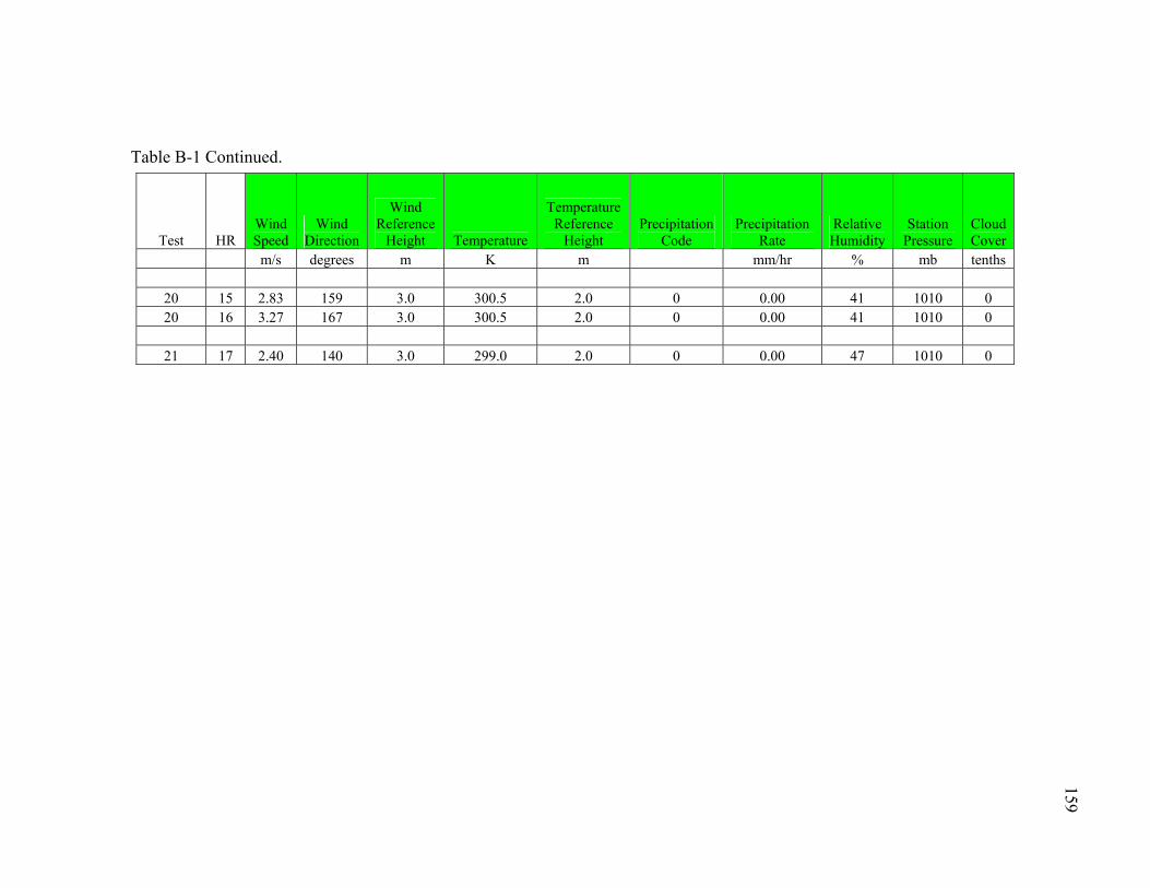
159
Table B-1 Continued.
Test HR Wind Speed
Wind Direction
Wind Reference
Height Temperature
Temperature Reference
Height Precipitation
Code Precipitation
Rate Relative
Humidity Station
Pressure Cloud Cover
m/s degrees m K m mm/hr % mb tenths
20 15 2.83 159 3.0 300.5 2.0 0 0.00 41 1010 0 20 16 3.27 167 3.0 300.5 2.0 0 0.00 41 1010 0
21 17 2.40 140 3.0 299.0 2.0 0 0.00 47 1010 0
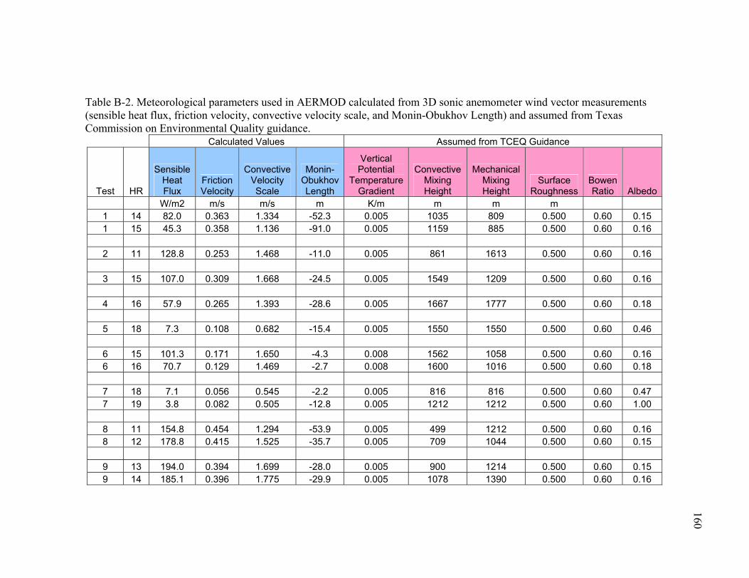
160
Table B-2. Meteorological parameters used in AERMOD calculated from 3D sonic anemometer wind vector measurements (sensible heat flux, friction velocity, convective velocity scale, and Monin-Obukhov Length) and assumed from Texas Commission on Environmental Quality guidance.
Calculated Values Assumed from TCEQ Guidance
Test HR
Sensible Heat Flux
Friction Velocity
Convective Velocity Scale
Monin-Obukhov Length
Vertical Potential
Temperature Gradient
Convective Mixing Height
Mechanical Mixing Height
Surface Roughness
Bowen Ratio Albedo
W/m2 m/s m/s m K/m m m m 1 14 82.0 0.363 1.334 -52.3 0.005 1035 809 0.500 0.60 0.15 1 15 45.3 0.358 1.136 -91.0 0.005 1159 885 0.500 0.60 0.16 2 11 128.8 0.253 1.468 -11.0 0.005 861 1613 0.500 0.60 0.16 3 15 107.0 0.309 1.668 -24.5 0.005 1549 1209 0.500 0.60 0.16 4 16 57.9 0.265 1.393 -28.6 0.005 1667 1777 0.500 0.60 0.18 5 18 7.3 0.108 0.682 -15.4 0.005 1550 1550 0.500 0.60 0.46 6 15 101.3 0.171 1.650 -4.3 0.008 1562 1058 0.500 0.60 0.16 6 16 70.7 0.129 1.469 -2.7 0.008 1600 1016 0.500 0.60 0.18 7 18 7.1 0.056 0.545 -2.2 0.005 816 816 0.500 0.60 0.47 7 19 3.8 0.082 0.505 -12.8 0.005 1212 1212 0.500 0.60 1.00 8 11 154.8 0.454 1.294 -53.9 0.005 499 1212 0.500 0.60 0.16 8 12 178.8 0.415 1.525 -35.7 0.005 709 1044 0.500 0.60 0.15 9 13 194.0 0.394 1.699 -28.0 0.005 900 1214 0.500 0.60 0.15 9 14 185.1 0.396 1.775 -29.9 0.005 1078 1390 0.500 0.60 0.16

161
Table B-2 Continued. Calculated Values Assumed from TCEQ Guidance
Test HR
Sensible Heat Flux
Friction Velocity
Convective Velocity Scale
Monin-Obukhov Length
Vertical Potential
Temperature Gradient
Convective Mixing Height
Mechanical Mixing Height
Surface Roughness
Bowen Ratio Albedo
W/m2 m/s m/s m K/m m m m 10 15 165.0 0.440 1.767 -45.9 0.005 1189 1383 0.500 0.60 0.16
11 17 12.2 0.438 0.764 -612.0 0.005 1297 1323 0.500 0.60 0.25
12 19 -29.2 0.280 -0.740 67.1 0.005 495 495 0.500 0.60 1.00
13 13 141.5 0.533 1.586 -94.9 0.005 1001 357 0.500 0.60 0.15 13 14 135.1 0.552 1.626 -110.8 0.005 1131 1050 0.500 0.60 0.15
14 15 86.5 0.592 1.445 -212.9 0.006 1238 525 0.500 0.60 0.16
15 16 44.4 0.603 1.179 -438.7 0.006 1310 855 0.500 0.60 0.18
16* 16 53.1 1.101 1.203 -2233.9 0.005 1165 2648 0.500 0.60 0.20 16* 17 20.0 1.031 0.875 -4856.6 0.005 1187 2422 0.500 0.60 0.29
17 11 133.5 0.092 0.986 -0.5 0.005 258 836 0.500 0.60 0.16 17 12 122.2 0.159 1.001 -3.0 0.005 296 1550 0.500 0.60 0.16
*3D sonic anemometer data was not available for test 16 and all values were assumed from TCEQ guidance.

162
Table B-2 Continued. Calculated Values Assumed from TCEQ Guidance
Test HR
Sensible Heat Flux
Friction Velocity
Convective Velocity
Scale
Monin-Obukhov Length
Vertical Potential
Temperature Gradient
Convective Mixing Height
Mechanical Mixing Height
Surface Roughness
Bowen Ratio Albedo
W/m2 m/s m/s m K/m m m m 18 14 194.0 0.488 1.263 -53.7 0.005 372 808 0.500 0.60 0.16 18 15 95.6 0.182 1.022 -5.7 0.005 401 1545 0.500 0.60 0.17 18 16 47.2 0.151 0.819 -6.5 0.005 420 1316 0.500 0.60 0.20 18 17 11.6 0.173 0.469 -40.0 0.005 320 684 0.500 0.60 0.29
19 12 145.0 0.149 1.091 -2.0 0.006 320 809 0.500 0.60 0.16 19 13 166.1 0.066 1.218 -0.2 0.006 390 1139 0.500 0.60 0.16 19 14 155.6 0.072 1.253 -0.2 0.006 455 822 0.500 0.60 0.16
20 15 106.8 0.200 1.148 -6.7 0.006 507 1132 0.500 0.60 0.17 20 16 54.7 0.227 0.966 -19.1 0.005 591 1152 0.500 0.60 0.20
21 17 3.7 0.186 0.396 -153.6 0.005 595 1295 0.500 0.60 0.30
163
APPENDIX C
TSP AND PM10 CONCENTRATION MEASUREMENTS TAKEN DURING THE
SAMPLING EVENTS DURING 2006 AND 2007
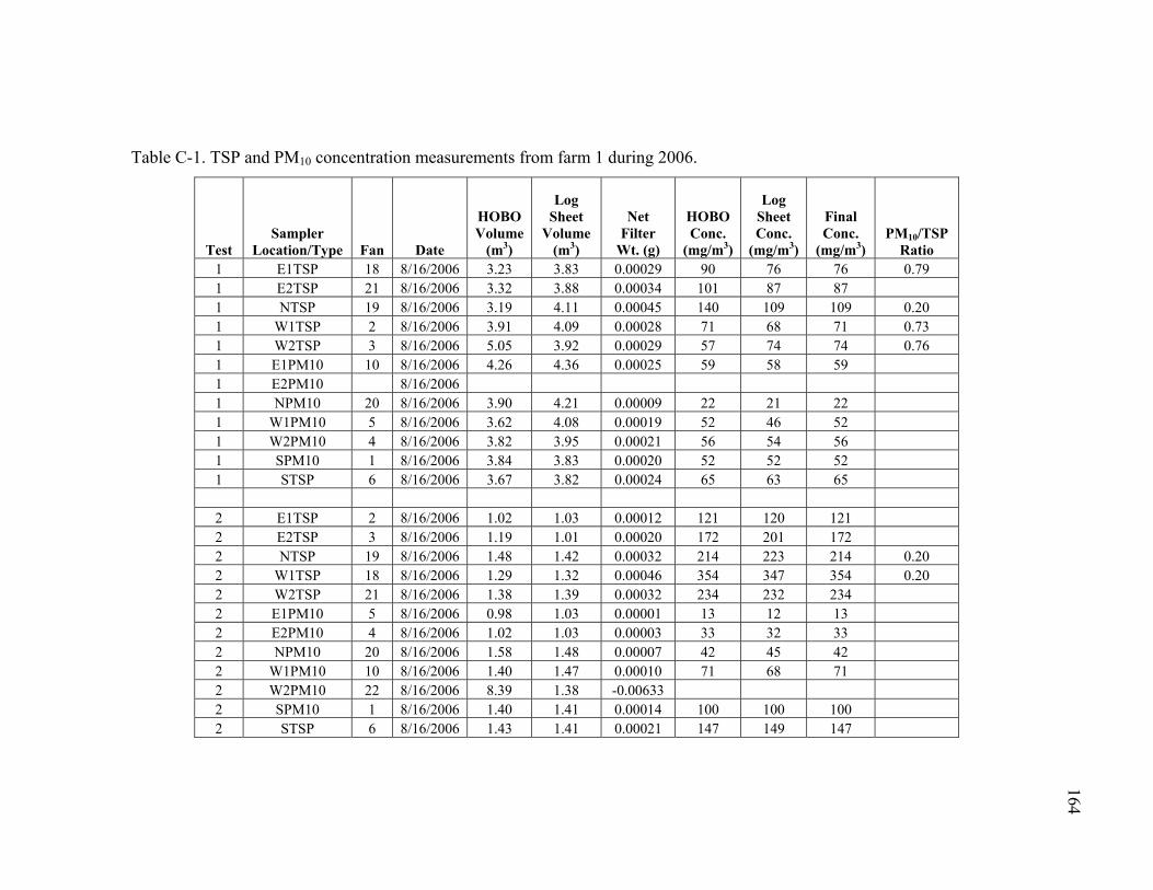
164
Table C-1. TSP and PM10 concentration measurements from farm 1 during 2006.
Test Sampler
Location/Type Fan Date
HOBO Volume
(m3)
Log Sheet
Volume (m3)
Net Filter
Wt. (g)
HOBO Conc.
(mg/m3)
Log Sheet Conc.
(mg/m3)
Final Conc.
(mg/m3) PM10/TSP
Ratio 1 E1TSP 18 8/16/2006 3.23 3.83 0.00029 90 76 76 0.79 1 E2TSP 21 8/16/2006 3.32 3.88 0.00034 101 87 87 1 NTSP 19 8/16/2006 3.19 4.11 0.00045 140 109 109 0.20 1 W1TSP 2 8/16/2006 3.91 4.09 0.00028 71 68 71 0.73 1 W2TSP 3 8/16/2006 5.05 3.92 0.00029 57 74 74 0.76 1 E1PM10 10 8/16/2006 4.26 4.36 0.00025 59 58 59 1 E2PM10 8/16/2006 1 NPM10 20 8/16/2006 3.90 4.21 0.00009 22 21 22 1 W1PM10 5 8/16/2006 3.62 4.08 0.00019 52 46 52 1 W2PM10 4 8/16/2006 3.82 3.95 0.00021 56 54 56 1 SPM10 1 8/16/2006 3.84 3.83 0.00020 52 52 52 1 STSP 6 8/16/2006 3.67 3.82 0.00024 65 63 65 2 E1TSP 2 8/16/2006 1.02 1.03 0.00012 121 120 121 2 E2TSP 3 8/16/2006 1.19 1.01 0.00020 172 201 172 2 NTSP 19 8/16/2006 1.48 1.42 0.00032 214 223 214 0.20 2 W1TSP 18 8/16/2006 1.29 1.32 0.00046 354 347 354 0.20 2 W2TSP 21 8/16/2006 1.38 1.39 0.00032 234 232 234 2 E1PM10 5 8/16/2006 0.98 1.03 0.00001 13 12 13 2 E2PM10 4 8/16/2006 1.02 1.03 0.00003 33 32 33 2 NPM10 20 8/16/2006 1.58 1.48 0.00007 42 45 42 2 W1PM10 10 8/16/2006 1.40 1.47 0.00010 71 68 71 2 W2PM10 22 8/16/2006 8.39 1.38 -0.00633 2 SPM10 1 8/16/2006 1.40 1.41 0.00014 100 100 100 2 STSP 6 8/16/2006 1.43 1.41 0.00021 147 149 147
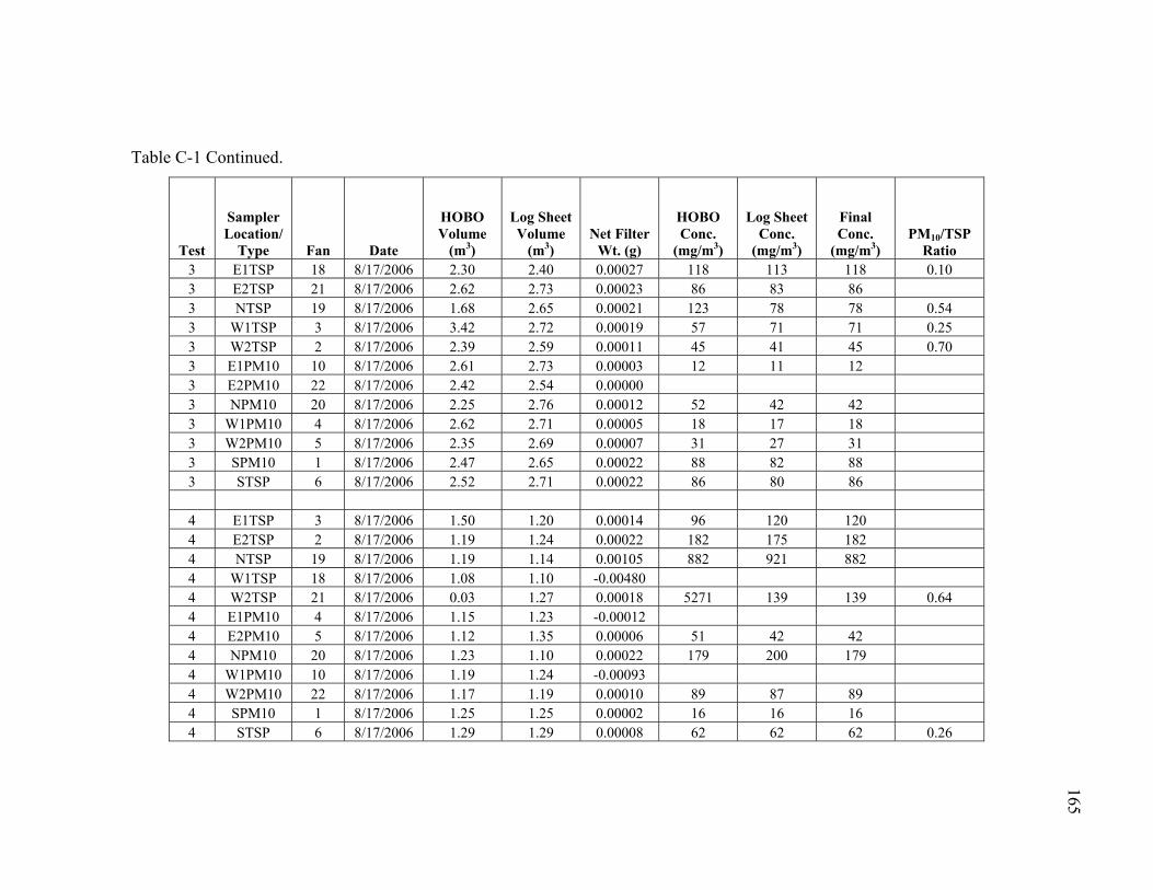
165
Table C-1 Continued.
Test
Sampler Location/
Type Fan Date
HOBO Volume
(m3)
Log Sheet Volume
(m3) Net Filter
Wt. (g)
HOBO Conc.
(mg/m3)
Log Sheet Conc.
(mg/m3)
Final Conc.
(mg/m3) PM10/TSP
Ratio 3 E1TSP 18 8/17/2006 2.30 2.40 0.00027 118 113 118 0.10 3 E2TSP 21 8/17/2006 2.62 2.73 0.00023 86 83 86 3 NTSP 19 8/17/2006 1.68 2.65 0.00021 123 78 78 0.54 3 W1TSP 3 8/17/2006 3.42 2.72 0.00019 57 71 71 0.25 3 W2TSP 2 8/17/2006 2.39 2.59 0.00011 45 41 45 0.70 3 E1PM10 10 8/17/2006 2.61 2.73 0.00003 12 11 12 3 E2PM10 22 8/17/2006 2.42 2.54 0.00000 3 NPM10 20 8/17/2006 2.25 2.76 0.00012 52 42 42 3 W1PM10 4 8/17/2006 2.62 2.71 0.00005 18 17 18 3 W2PM10 5 8/17/2006 2.35 2.69 0.00007 31 27 31 3 SPM10 1 8/17/2006 2.47 2.65 0.00022 88 82 88 3 STSP 6 8/17/2006 2.52 2.71 0.00022 86 80 86 4 E1TSP 3 8/17/2006 1.50 1.20 0.00014 96 120 120 4 E2TSP 2 8/17/2006 1.19 1.24 0.00022 182 175 182 4 NTSP 19 8/17/2006 1.19 1.14 0.00105 882 921 882 4 W1TSP 18 8/17/2006 1.08 1.10 -0.00480 4 W2TSP 21 8/17/2006 0.03 1.27 0.00018 5271 139 139 0.64 4 E1PM10 4 8/17/2006 1.15 1.23 -0.00012 4 E2PM10 5 8/17/2006 1.12 1.35 0.00006 51 42 42 4 NPM10 20 8/17/2006 1.23 1.10 0.00022 179 200 179 4 W1PM10 10 8/17/2006 1.19 1.24 -0.00093 4 W2PM10 22 8/17/2006 1.17 1.19 0.00010 89 87 89 4 SPM10 1 8/17/2006 1.25 1.25 0.00002 16 16 16 4 STSP 6 8/17/2006 1.29 1.29 0.00008 62 62 62 0.26

166
Table C-1 Continued.
Test
Sampler Location/
Type Fan Date
HOBO Volume
(m3)
Log Sheet Volume
(m3) Net Filter
Wt. (g)
HOBO Conc.
(mg/m3)
Log Sheet Conc.
(mg/m3)
Final Conc.
(mg/m3) PM10/TSP
Ratio 5 E1TSP 18 8/18/2006 3.43 3.98 3600 0.00023 67 58 58 5 E2TSP 21 8/18/2006 0.00 4.11 3599 0.00015 37 37 5 W1TSP 2 8/18/2006 3.67 3.96 3602 0.00028 77 71 77 5 W2TSP 3 8/18/2006 5.17 4.04 3603 0.00045 87 111 111 5 STSP 6 8/18/2006 3.93 4.20 3604 0.00121 307 287 307 5 E1PM10 10 8/18/2006 3.85 4.11 3606 0.00003 8 7 8 5 E2PM10 22 8/18/2006 3.65 3.89 3605 0.00003 7 7 7 5 W1PM10 5 8/18/2006 3.17 3.99 3608 0.00009 27 22 22 5 W2PM10 4 8/18/2006 3.75 3.92 3609 0.00013 34 32 34 5 SPM10 1 8/18/2006 4.08 4.08 3610 0.00048 117 117 117 5 NPM10 20 8/18/2006 3.03 3607 0.00000 0 5 NTSP 19 8/18/2006 2.26 3601 0.00016 69 69 6 E1TSP 3 8/18/2006 1.53 1.01 3614 0.00031 200 303 303 6 E2TSP 2 8/18/2006 1.08 0.95 3613 0.00013 120 137 120 6 NTSP 19 8/18/2006 0.73 1.03 3615 0.00018 242 172 172 6 W1TSP 21 8/18/2006 0.00 1.11 3616 0.00026 235 235 6 W2TSP 18 8/18/2006 1.01 1.02 3617 0.00033 330 326 330 6 E1PM10 4 8/18/2006 1.06 0.98 3612 0.00005 47 51 47 6 E2PM10 5 8/18/2006 0.99 0.94 3611 0.00004 44 46 44 6 NPM10 20 8/18/2006 1.12 1.10 3625 -0.00003 6 W1PM10 22 8/18/2006 1.08 1.05 3626 0.00009 86 89 86 6 W2PM10 10 8/18/2006 1.17 1.11 3627 0.00017 145 153 145 6 SPM10 1 8/18/2006 1.20 1.19 3628 0.00008 67 67 67 6 STSP 6 8/18/2006 0.00 1.20 3618 0.00000 0
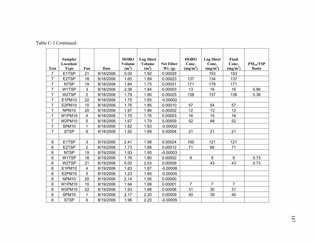
167
Table C-1 Continued.
Test
Sampler Location/
Type Fan Date
HOBO Volume
(m3)
Log Sheet Volume
(m3) Net Filter
Wt. (g)
HOBO Conc.
(mg/m3)
Log Sheet Conc.
(mg/m3)
Final Conc.
(mg/m3) PM10/TSP
Ratio 7 E1TSP 21 8/18/2006 0.00 1.92 0.00029 153 153 7 E2TSP 18 8/18/2006 1.65 1.69 0.00023 137 134 137 7 NTSP 19 8/18/2006 1.84 1.75 0.00031 171 179 171 7 W1TSP 3 8/18/2006 2.38 1.84 0.00003 13 16 16 0.96 7 W2TSP 2 8/18/2006 1.79 1.80 0.00025 138 137 138 0.38 7 E1PM10 22 8/18/2006 1.75 1.85 -0.00002 7 E2PM10 10 8/18/2006 1.76 1.85 0.00010 57 54 57 7 NPM10 20 8/18/2006 1.97 1.86 0.00002 12 13 12 7 W1PM10 4 8/18/2006 1.70 1.76 0.00003 16 15 16 7 W2PM10 5 8/18/2006 1.67 1.79 0.00009 52 48 52 7 SPM10 1 8/18/2006 1.82 1.83 -0.00002 7 STSP 6 8/18/2006 1.92 1.89 0.00004 21 21 21 8 E1TSP 3 8/19/2006 2.41 1.98 0.00024 100 121 121 8 E2TSP 2 8/19/2006 1.73 1.88 0.00012 71 66 71 8 NTSP 19 8/19/2006 1.93 1.95 -0.00003 8 W1TSP 18 8/19/2006 1.76 1.80 0.00002 9 9 9 0.73 8 W2TSP 21 8/19/2006 0.00 2.03 0.00009 43 43 0.73 8 E1PM10 4 8/19/2006 1.83 1.87 -0.00008 8 E2PM10 5 8/19/2006 1.23 1.90 -0.00005 8 NPM10 20 8/19/2006 2.14 1.95 0.00000 8 W1PM10 10 8/19/2006 1.94 1.99 0.00001 7 7 7 8 W2PM10 22 8/19/2006 1.93 1.98 0.00006 31 30 31 8 SPM10 1 8/19/2006 2.17 2.20 0.00009 40 39 40 8 STSP 6 8/19/2006 1.96 2.23 -0.00005
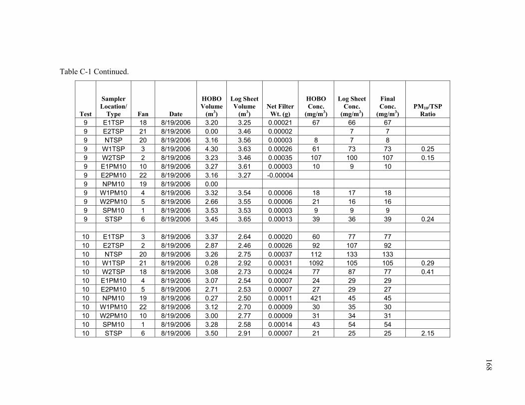
168
Table C-1 Continued.
Test
Sampler Location/
Type Fan Date
HOBO Volume
(m3)
Log Sheet Volume
(m3) Net Filter
Wt. (g)
HOBO Conc.
(mg/m3)
Log Sheet Conc.
(mg/m3)
Final Conc.
(mg/m3) PM10/TSP
Ratio 9 E1TSP 18 8/19/2006 3.20 3.25 0.00021 67 66 67 9 E2TSP 21 8/19/2006 0.00 3.46 0.00002 7 7 9 NTSP 20 8/19/2006 3.16 3.56 0.00003 8 7 8 9 W1TSP 3 8/19/2006 4.30 3.63 0.00026 61 73 73 0.25 9 W2TSP 2 8/19/2006 3.23 3.46 0.00035 107 100 107 0.15 9 E1PM10 10 8/19/2006 3.27 3.61 0.00003 10 9 10 9 E2PM10 22 8/19/2006 3.16 3.27 -0.00004 9 NPM10 19 8/19/2006 0.00 9 W1PM10 4 8/19/2006 3.32 3.54 0.00006 18 17 18 9 W2PM10 5 8/19/2006 2.66 3.55 0.00006 21 16 16 9 SPM10 1 8/19/2006 3.53 3.53 0.00003 9 9 9 9 STSP 6 8/19/2006 3.45 3.65 0.00013 39 36 39 0.24
10 E1TSP 3 8/19/2006 3.37 2.64 0.00020 60 77 77 10 E2TSP 2 8/19/2006 2.87 2.46 0.00026 92 107 92 10 NTSP 20 8/19/2006 3.26 2.75 0.00037 112 133 133 10 W1TSP 21 8/19/2006 0.28 2.92 0.00031 1092 105 105 0.29 10 W2TSP 18 8/19/2006 3.08 2.73 0.00024 77 87 77 0.41 10 E1PM10 4 8/19/2006 3.07 2.54 0.00007 24 29 29 10 E2PM10 5 8/19/2006 2.71 2.53 0.00007 27 29 27 10 NPM10 19 8/19/2006 0.27 2.50 0.00011 421 45 45 10 W1PM10 22 8/19/2006 3.12 2.70 0.00009 30 35 30 10 W2PM10 10 8/19/2006 3.00 2.77 0.00009 31 34 31 10 SPM10 1 8/19/2006 3.28 2.58 0.00014 43 54 54 10 STSP 6 8/19/2006 3.50 2.91 0.00007 21 25 25 2.15

169
Table C-2. TSP and PM10 concentration measurements taken at farm 2 during 2006.
Test
Sampler Location/
Type Fan Date
HOBO Volume
(m3)
Log Sheet
Volume (m3)
Net Filter Wt. (g)
HOBO Conc.
(mg/m3) LS Conc. (mg/m3)
Final Conc. (mg/m3)
PM10/TSP Ratio
1 D1TSP 2 9/1/2006 0.00 1.54 0.00009 0 58 58 0.36 1 D2TSP 22 9/1/2006 1.15 1.41 0.00007 58 47 47 0.38 1 D3TSP 1 9/1/2006 1.41 1.41 0.00006 45 45 45 0.98 1 D4TSP 5 9/1/2006 0.00 1.50 0.00007 0 49 49 1.04 1 D5TSP 21 9/1/2006 1.43 1.48 0.00019 133 129 133 0.32 1 D1PM10 4 9/1/2006 1.44 1.54 0.00003 21 20 21 1 D2PM10 17 9/1/2006 1.50 1.46 0.00003 18 18 18 1 D3PM10 20 9/1/2006 1.44 1.61 0.00006 44 39 44 1 D4PM10 3 9/1/2006 0.03 1.52 0.00008 2730 51 51 1 D5PM10 18 9/1/2006 1.49 1.48 0.00006 42 43 42 1 U1TSP 19 9/1/2006 0.73 0.00 0.00003 46 0 46 1 U1PM10 6 9/1/2006 0.00 1.75 0.00008 0 46 46 2 D1TSP 2 9/1/2006 0.00 0.00 0.00001 0 0 2 D2TSP 1 9/1/2006 2.35 2.36 0.00016 70 69 70 0.98 2 D3TSP 21 9/1/2006 2.39 2.44 0.00011 45 44 45 0.80 2 D4TSP 22 9/1/2006 0.30 2.36 0.00001 23 3 2 D5TSP 5 9/1/2006 0.00 0.00 0.00005 0 0 2 D1PM10 4 9/1/2006 0.71 0.00 0.00000 5 0 2 D2PM10 20 9/1/2006 2.60 2.69 0.00018 68 66 68 2 D3PM10 18 9/1/2006 2.42 2.49 0.00009 36 35 36 2 D4PM10 17 9/1/2006 0.24 0.00 0.00003 123 0 123 2 D5PM10 3 9/1/2006 0.33 0.00 0.00000 10 0 10 2 U1TSP 19 9/1/2006 0.83 0.00 0.00000 0 0 2 U1PM10 6 9/1/2006 0.00 0.00 0.00006 0 0
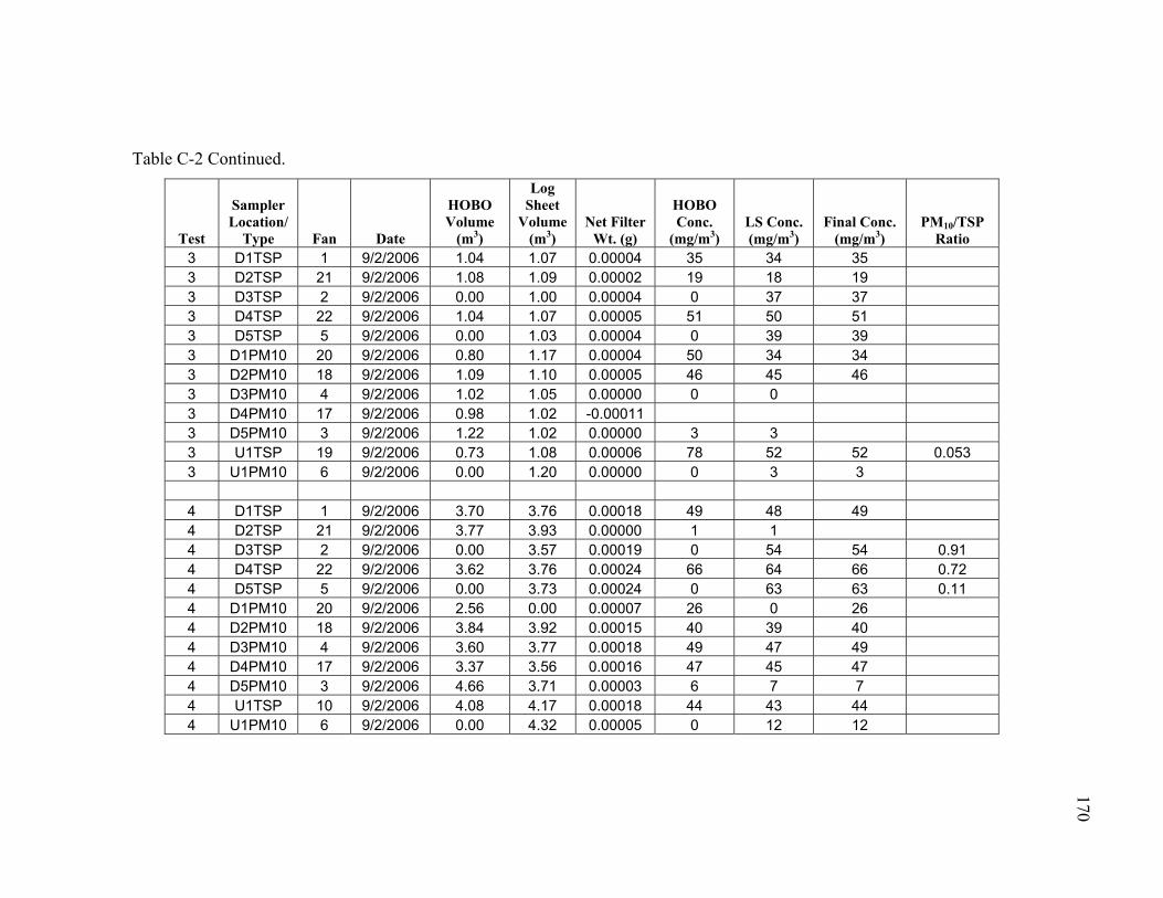
170
Table C-2 Continued.
Test
Sampler Location/
Type Fan Date
HOBO Volume
(m3)
Log Sheet
Volume (m3)
Net Filter Wt. (g)
HOBO Conc.
(mg/m3) LS Conc. (mg/m3)
Final Conc. (mg/m3)
PM10/TSP Ratio
3 D1TSP 1 9/2/2006 1.04 1.07 0.00004 35 34 35 3 D2TSP 21 9/2/2006 1.08 1.09 0.00002 19 18 19 3 D3TSP 2 9/2/2006 0.00 1.00 0.00004 0 37 37 3 D4TSP 22 9/2/2006 1.04 1.07 0.00005 51 50 51 3 D5TSP 5 9/2/2006 0.00 1.03 0.00004 0 39 39 3 D1PM10 20 9/2/2006 0.80 1.17 0.00004 50 34 34 3 D2PM10 18 9/2/2006 1.09 1.10 0.00005 46 45 46 3 D3PM10 4 9/2/2006 1.02 1.05 0.00000 0 0 3 D4PM10 17 9/2/2006 0.98 1.02 -0.00011 3 D5PM10 3 9/2/2006 1.22 1.02 0.00000 3 3 3 U1TSP 19 9/2/2006 0.73 1.08 0.00006 78 52 52 0.053 3 U1PM10 6 9/2/2006 0.00 1.20 0.00000 0 3 3 4 D1TSP 1 9/2/2006 3.70 3.76 0.00018 49 48 49 4 D2TSP 21 9/2/2006 3.77 3.93 0.00000 1 1 4 D3TSP 2 9/2/2006 0.00 3.57 0.00019 0 54 54 0.91 4 D4TSP 22 9/2/2006 3.62 3.76 0.00024 66 64 66 0.72 4 D5TSP 5 9/2/2006 0.00 3.73 0.00024 0 63 63 0.11 4 D1PM10 20 9/2/2006 2.56 0.00 0.00007 26 0 26 4 D2PM10 18 9/2/2006 3.84 3.92 0.00015 40 39 40 4 D3PM10 4 9/2/2006 3.60 3.77 0.00018 49 47 49 4 D4PM10 17 9/2/2006 3.37 3.56 0.00016 47 45 47 4 D5PM10 3 9/2/2006 4.66 3.71 0.00003 6 7 7 4 U1TSP 10 9/2/2006 4.08 4.17 0.00018 44 43 44 4 U1PM10 6 9/2/2006 0.00 4.32 0.00005 0 12 12

171
Table C-2 Continued.
Test
Sampler Location/
Type Fan Date
HOBO Volume
(m3)
Log Sheet
Volume (m3)
Net Filter Wt. (g)
HOBO Conc.
(mg/m3) LS Conc. (mg/m3)
Final Conc. (mg/m3)
PM10/TSP Ratio
5 D1TSP 1 9/2/2006 2.57 2.60 0.00044 170 168 170 5 D2TSP 21 9/2/2006 2.75 2.69 0.00053 193 197 193 0.47 5 D3TSP 2 9/2/2006 0.00 2.55 0.00052 0 205 205 0.57 5 D4TSP 22 9/2/2006 2.80 2.60 0.00057 202 218 202 0.62 5 D5TSP 5 9/2/2006 0.00 2.80 0.00049 0 176 176 0.65 5 D1PM10 20 9/2/2006 2.81 2.80 0.00034 121 121 121 5 D2PM10 18 9/2/2006 2.78 2.78 0.00025 91 91 91 5 D3PM10 4 9/2/2006 2.63 2.69 0.00031 116 114 116 5 D4PM10 17 9/2/2006 2.57 2.56 0.00032 125 125 125 5 D5PM10 3 9/2/2006 3.43 2.84 0.00033 95 115 115 5 U1TSP 10 9/2/2006 1.39 2.80 0.00026 190 94 94 5 U1PM10 6 9/2/2006 0.00 0.00 0.00020 0 0 6 D1TSP 1 9/3/2006 3.81 3.82 0.00018 46 46 46 6 D2TSP 21 9/3/2006 3.86 4.05 0.00018 47 44 47 0.86 6 D3TSP 2 9/3/2006 0.00 3.72 0.00016 0 42 42 0.90 6 D4TSP 22 9/3/2006 3.84 4.00 0.00023 59 57 59 6 D5TSP 5 9/3/2006 0.00 4.00 0.00018 0 44 44 0.62 6 D1PM10 20 9/3/2006 2.23 0.00 0.00002 9 0 9 6 D2PM10 18 9/3/2006 3.80 3.96 0.00015 40 39 40 6 D3PM10 4 9/3/2006 3.70 3.92 0.00014 38 36 38 6 D4PM10 17 9/3/2006 3.55 3.80 0.00000 0 0 6 D5PM10 3 9/3/2006 4.85 3.98 0.00011 23 28 28 6 U1TSP 10 9/3/2006 4.01 4.15 0.00022 54 52 54 6 U1PM10 6 9/3/2006 0.00 4.25 0.00000 0 1
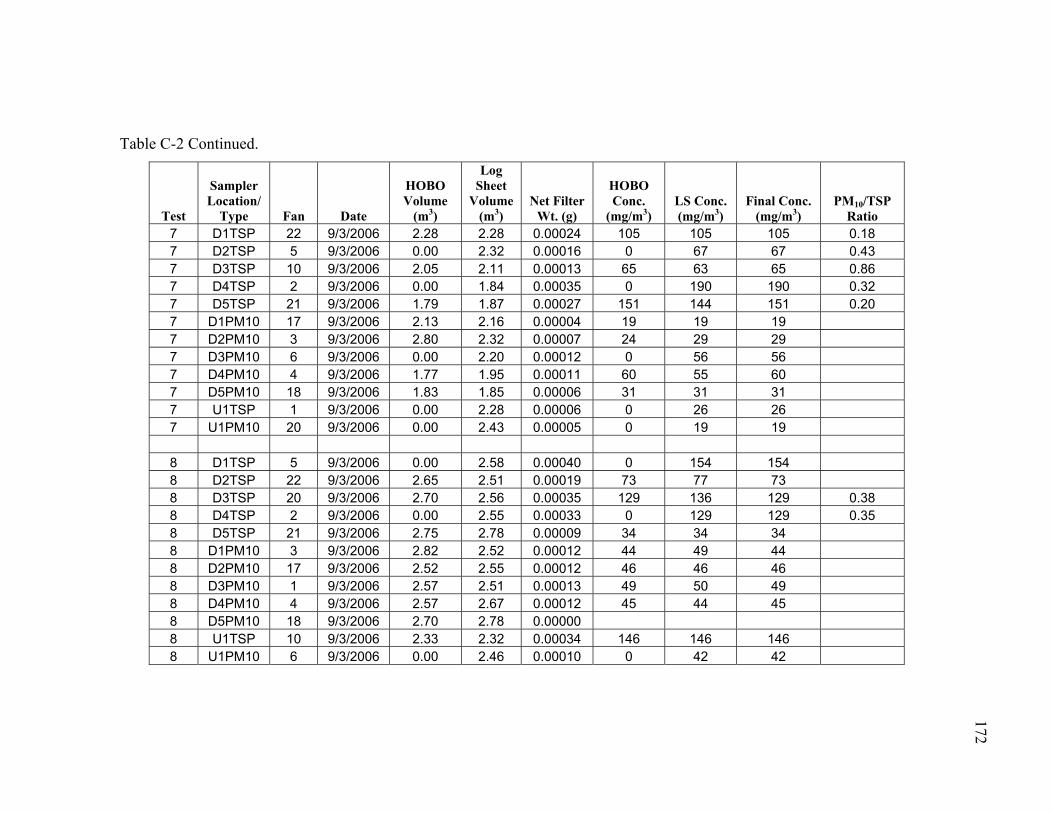
172
Table C-2 Continued.
Test
Sampler Location/
Type Fan Date
HOBO Volume
(m3)
Log Sheet
Volume (m3)
Net Filter Wt. (g)
HOBO Conc.
(mg/m3) LS Conc. (mg/m3)
Final Conc. (mg/m3)
PM10/TSP Ratio
7 D1TSP 22 9/3/2006 2.28 2.28 0.00024 105 105 105 0.18 7 D2TSP 5 9/3/2006 0.00 2.32 0.00016 0 67 67 0.43 7 D3TSP 10 9/3/2006 2.05 2.11 0.00013 65 63 65 0.86 7 D4TSP 2 9/3/2006 0.00 1.84 0.00035 0 190 190 0.32 7 D5TSP 21 9/3/2006 1.79 1.87 0.00027 151 144 151 0.20 7 D1PM10 17 9/3/2006 2.13 2.16 0.00004 19 19 19 7 D2PM10 3 9/3/2006 2.80 2.32 0.00007 24 29 29 7 D3PM10 6 9/3/2006 0.00 2.20 0.00012 0 56 56 7 D4PM10 4 9/3/2006 1.77 1.95 0.00011 60 55 60 7 D5PM10 18 9/3/2006 1.83 1.85 0.00006 31 31 31 7 U1TSP 1 9/3/2006 0.00 2.28 0.00006 0 26 26 7 U1PM10 20 9/3/2006 0.00 2.43 0.00005 0 19 19 8 D1TSP 5 9/3/2006 0.00 2.58 0.00040 0 154 154 8 D2TSP 22 9/3/2006 2.65 2.51 0.00019 73 77 73 8 D3TSP 20 9/3/2006 2.70 2.56 0.00035 129 136 129 0.38 8 D4TSP 2 9/3/2006 0.00 2.55 0.00033 0 129 129 0.35 8 D5TSP 21 9/3/2006 2.75 2.78 0.00009 34 34 34 8 D1PM10 3 9/3/2006 2.82 2.52 0.00012 44 49 44 8 D2PM10 17 9/3/2006 2.52 2.55 0.00012 46 46 46 8 D3PM10 1 9/3/2006 2.57 2.51 0.00013 49 50 49 8 D4PM10 4 9/3/2006 2.57 2.67 0.00012 45 44 45 8 D5PM10 18 9/3/2006 2.70 2.78 0.00000 8 U1TSP 10 9/3/2006 2.33 2.32 0.00034 146 146 146 8 U1PM10 6 9/3/2006 0.00 2.46 0.00010 0 42 42
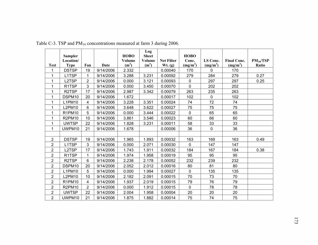
173
Table C-3. TSP and PM10 concentrations measured at farm 3 during 2006.
Test
Sampler Location/
Type Fan Date
HOBO Volume
(m3)
Log Sheet
Volume (m3)
Net Filter Wt. (g)
HOBO Conc.
(mg/m3) LS Conc. (mg/m3)
Final Conc. (mg/m3)
PM10/TSP Ratio
1 DSTSP 19 9/14/2006 2.332 0.00040 170 0 170 1 L1TSP 1 9/14/2006 3.288 3.231 0.00092 279 284 279 0.27 1 L2TSP 2 9/14/2006 0.000 3.121 0.00093 0 297 297 0.25 1 R1TSP 3 9/14/2006 0.000 3.450 0.00070 0 202 202 1 R2TSP 17 9/14/2006 2.987 3.342 0.00079 263 235 263 1 DSPM10 20 9/14/2006 1.672 0.00017 102 0 102 1 L1PM10 4 9/14/2006 3.228 3.351 0.00024 74 72 74 1 L2PM10 6 9/14/2006 3.648 3.622 0.00027 75 75 75 1 R1PM10 5 9/14/2006 0.000 3.444 0.00022 0 65 65 1 R2PM10 10 9/14/2006 3.861 3.546 0.00023 60 66 60 1 UWTSP 22 9/14/2006 1.828 3.231 0.00011 58 33 33 1 UWPM10 21 9/14/2006 1.678 0.00006 36 0 36 2 DSTSP 19 9/14/2006 1.965 1.893 0.00032 163 169 163 0.49 2 L1TSP 3 9/14/2006 0.000 2.071 0.00030 0 147 147 2 L2TSP 17 9/14/2006 1.743 1.911 0.00032 184 167 184 0.38 2 R1TSP 1 9/14/2006 1.974 1.958 0.00019 95 95 95 2 R2TSP 6 9/14/2006 2.238 2.178 0.00052 232 239 232 2 DSPM10 20 9/14/2006 2.052 2.012 0.00016 80 81 80 2 L1PM10 5 9/14/2006 0.000 1.994 0.00027 0 135 135 2 L2PM10 10 9/14/2006 2.182 2.091 0.00015 70 73 70 2 R1PM10 4 9/14/2006 1.937 2.019 0.00015 79 76 79 2 R2PM10 2 9/14/2006 0.000 1.912 0.00015 0 78 78 2 UWTSP 22 9/14/2006 2.004 1.958 0.00004 20 20 20 2 UWPM10 21 9/14/2006 1.875 1.882 0.00014 75 74 75

174
Table C-3 Continued.
Test
Sampler Location/
Type Fan Date
HOBO Volume
(m3)
Log Sheet
Volume (m3)
Net Filter Wt. (g)
HOBO Conc.
(mg/m3) LS Conc. (mg/m3)
Final Conc. (mg/m3)
PM10/TSP Ratio
3 DSTSP 19 9/15/2006 4.392 4.278 0.00025 57 58 57 3 L1TSP 1 9/15/2006 4.205 4.235 0.00035 84 83 84 0.48 3 L2TSP 2 9/15/2006 0.000 4.072 0.00037 0 90 90 0.38 3 R1TSP 3 9/15/2006 0.000 4.264 0.00026 0 62 62 3 R2TSP 17 9/15/2006 3.552 4.008 0.00032 89 79 89 3 DSPM10 20 9/15/2006 3.331 4.405 0.00011 32 24 24 3 L1PM10 4 9/15/2006 4.091 4.302 0.00017 41 39 41 3 L2PM10 6 9/15/2006 4.617 4.596 0.00016 34 34 34 3 R1PM10 5 9/15/2006 0.000 4.201 0.00011 0 25 25 3 R2PM10 10 9/15/2006 4.502 4.254 0.00007 16 17 16 3 UWTSP 22 9/15/2006 4.393 4.235 0.00049 112 116 112 3 UWPM10 21 9/15/2006 4.188 4.397 0.00012 29 28 29
5 DSTSP 19 9/16/2006 1.080 1.541 0.00006 52 37 37 5 L1TSP 2 9/16/2006 0.000 1.556 0.00012 0 75 75 5 L2TSP 1 9/16/2006 1.491 1.556 0.00028 190 182 190 0.21 5 R1TSP 3 9/16/2006 0.000 1.833 0.00020 0 111 111 5 R2TSP 17 9/16/2006 1.553 1.750 0.00017 112 99 112 5 DSPM10 20 9/16/2006 1.255 1.603 0.00092 733 574 574 5 L1PM10 6 9/16/2006 1.425 1.568 0.00003 23 21 23 5 L2PM10 4 9/16/2006 1.448 1.502 0.00006 39 38 39 5 R1PM10 5 9/16/2006 0.000 1.810 0.00004 0 24 24 5 R2PM10 10 9/16/2006 1.967 1.885 0.00000 0 0 5 UWTSP 22 9/16/2006 1.537 1.556 0.00000 2 2 2 5 UWPM10 21 9/16/2006 1.541 1.622 0.00000 2 2 2
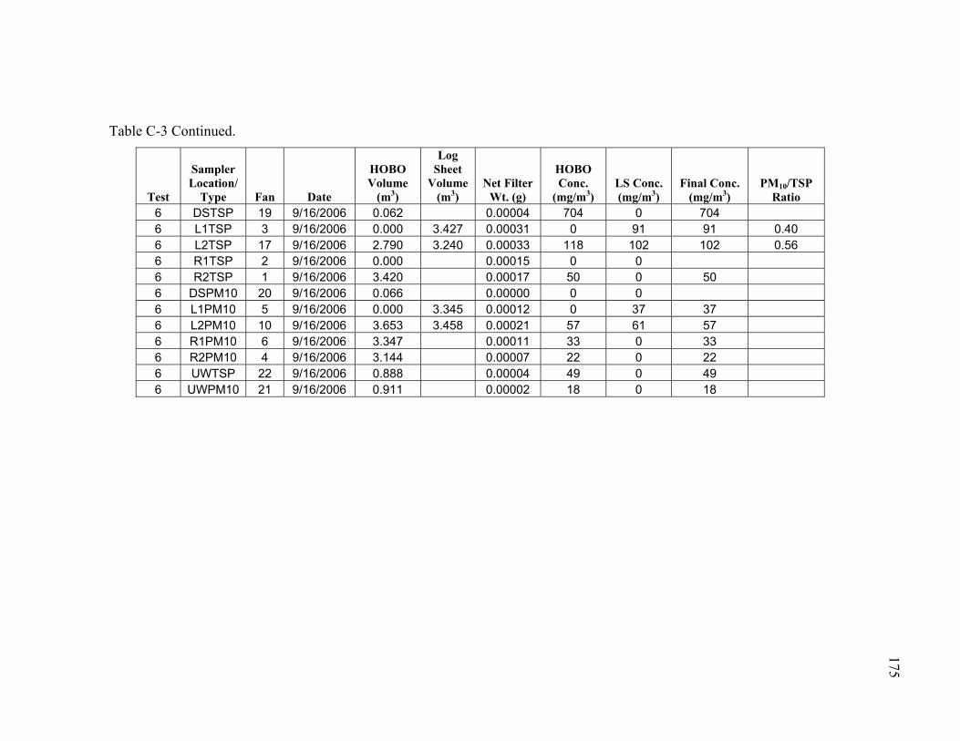
175
Table C-3 Continued.
Test
Sampler Location/
Type Fan Date
HOBO Volume
(m3)
Log Sheet
Volume (m3)
Net Filter Wt. (g)
HOBO Conc.
(mg/m3) LS Conc. (mg/m3)
Final Conc. (mg/m3)
PM10/TSP Ratio
6 DSTSP 19 9/16/2006 0.062 0.00004 704 0 704 6 L1TSP 3 9/16/2006 0.000 3.427 0.00031 0 91 91 0.40 6 L2TSP 17 9/16/2006 2.790 3.240 0.00033 118 102 102 0.56 6 R1TSP 2 9/16/2006 0.000 0.00015 0 0 6 R2TSP 1 9/16/2006 3.420 0.00017 50 0 50 6 DSPM10 20 9/16/2006 0.066 0.00000 0 0 6 L1PM10 5 9/16/2006 0.000 3.345 0.00012 0 37 37 6 L2PM10 10 9/16/2006 3.653 3.458 0.00021 57 61 57 6 R1PM10 6 9/16/2006 3.347 0.00011 33 0 33 6 R2PM10 4 9/16/2006 3.144 0.00007 22 0 22 6 UWTSP 22 9/16/2006 0.888 0.00004 49 0 49 6 UWPM10 21 9/16/2006 0.911 0.00002 18 0 18

176
Table C-4. TSP and PM10 concentrations measured at farm 3 during 2007.
Test Sampler
Type Easting
CoordinatesNorthing
Coordinates Fan
HOBO Volume
(m3)
Log Sheet
Volume (m3)
Net Filter
Wt. (g)
Final Conc.
(μg/m3)PM10/TSP
Ratio 1 TSP 747135 3382037 7 n/a 1.67 0.00016 94 0.66 1 TSP 747183 3382008 3 1.58 1.75 0.00025 160 0.62 1 TSP 747227 3382156 12 n/a 1.62 0.00024 150 0.77 1 TSP 747275 3382122 4 1.79 1.98 0.00025 141 0.86 1 TSP 747987 3381465 15 n/a 1.67 0.00010 58 0.55 1 PM10 747135 3382037 21 1.74 1.76 0.00011 61 1 PM10 747183 3382008 14 n/a 1.74 0.00017 100 1 PM10 747227 3382156 11 1.41 1.63 0.00016 116 1 PM10 747275 3382122 6 1.86 1.98 0.00023 122 1 PM10 747987 3381465 17 2.22 2.35 0.00007 32 2 TSP 747275 3381944 7 1.44 0.97 0.00009 65 2 TSP 747317 3381914 3 n/a 1.04 0.00015 144 0.67 2 TSP 747377 3382075 12 1.10 0.90 0.00016 149 0.90 2 TSP 747421 3382041 4 1.17 1.28 0.00021 183 2 TSP 747987 3381465 15 n/a 5.71 0.00014 25 0.73 2 PM10 747275 3381944 21 0.86 0.95 0.00009 101 2 PM10 747317 3381914 14 n/a 1.18 0.00011 96 2 PM10 747377 3382075 11 0.75 0.90 0.00010 133 2 PM10 747421 3382041 6 1.21 1.28 0.00011 94 2 PM10 747987 3381465 17 7.69 8.20 0.00014 18

177
Table C-4 Continued.
Test Sampler
Type Easting
CoordinatesNorthing
Coordinates Fan
HOBO Volume
(m3)
Log Sheet
Volume (m3)
Net Filter
Wt. (g)
Final Conc.
(μg/m3)PM10/TSP
Ratio 3 TSP 747469 3381743 7 0.92 0.75 0.00005 51 3 TSP 747518 3381714 3 n/a 0.82 0.00019 229 0.41 3 TSP 747532 3381825 12 0.93 0.76 0.00016 175 3 TSP 747574 3381790 4 0.84 0.91 0.00015 182 0.08 3 PM10 747469 3381743 21 0.67 0.73 0.00015 227 3 PM10 747518 3381714 14 n/a 0.93 0.00009 93 3 PM10 747532 3381825 11 0.70 0.76 0.00007 96 3 PM10 747574 3381790 6 0.91 0.94 0.00001 15 4 TSP 747510 3381712 3 n/a 0.75 0.00010 138 0.39 4 TSP 747554 3381677 7 1.19 1.00 0.00041 346 0.49 4 TSP 747572 3381787 4 0.75 0.81 0.00013 168 4 TSP 747614 3381759 12 1.20 0.97 0.00022 184 0.91 4 PM10 747510 3381712 14 n/a 0.86 0.00005 54 4 PM10 747554 3381677 21 0.93 0.92 0.00016 168 4 PM10 747572 3381787 6 0.82 0.82 0.00006 69 4 PM10 747614 3381759 11 0.94 1.01 0.00016 168

178
Table C-4 Continued.
Test Sampler
Type Easting
CoordinatesNorthing
Coordinates Fan
HOBO Volume
(m3)
Log Sheet
Volume (m3)
Net Filter
Wt. (g)
Final Conc.
(μg/m3)PM10/TSP
Ratio 5 TSP 747752 3381488 3 n/a 0.94 0.00006 64 5 TSP 747800 3381550 4 1.08 1.12 0.00018 164 5 TSP 747804 3381462 7 1.32 1.07 0.00012 94 0.36 5 TSP 747845 3381517 12 1.25 1.01 0.00011 91 0.99 5 PM10 747752 3381488 14 n/a 1.09 0.00007 64 5 PM10 747800 3381550 6 1.13 1.13 0.00004 38 5 PM10 747804 3381462 21 1.08 1.04 0.00004 34 5 PM10 747845 3381517 11 0.96 1.00 0.00009 90 6 TSP 747223 3382056 7 2.65 1.86 0.00027 101 0.61 6 TSP 747268 3382021 3 n/a 1.79 0.00017 95 6 TSP 747304 3382160 12 2.15 1.83 0.00043 198 0.27 6 TSP 747350 3382129 4 2.01 2.15 0.00026 127 6 TSP 747987 3381465 15 n/a 3.35 0.00012 35 0.36 6 PM10 747223 3382056 21 1.91 1.86 0.00012 61 6 PM10 747268 3382021 14 n/a 2.01 0.00016 81 6 PM10 747304 3382160 11 2.26 1.83 0.00012 53 6 PM10 747350 3382129 6 n/a 2.16 0.00015 71 6 PM10 747987 3381465 17 4.59 4.84 0.00006 12
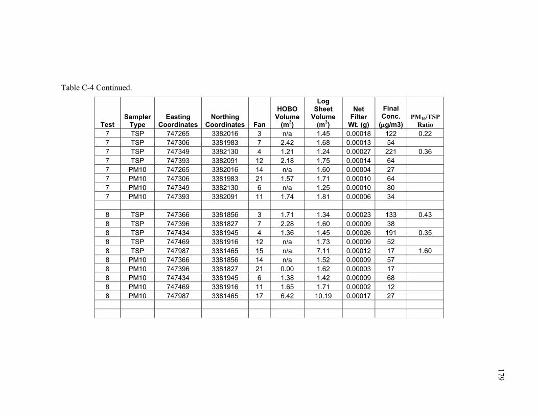
179
Table C-4 Continued.
Test Sampler
Type Easting
CoordinatesNorthing
Coordinates Fan
HOBO Volume
(m3)
Log Sheet
Volume (m3)
Net Filter
Wt. (g)
Final Conc.
(μg/m3)PM10/TSP
Ratio 7 TSP 747265 3382016 3 n/a 1.45 0.00018 122 0.22 7 TSP 747306 3381983 7 2.42 1.68 0.00013 54 7 TSP 747349 3382130 4 1.21 1.24 0.00027 221 0.36 7 TSP 747393 3382091 12 2.18 1.75 0.00014 64 7 PM10 747265 3382016 14 n/a 1.60 0.00004 27 7 PM10 747306 3381983 21 1.57 1.71 0.00010 64 7 PM10 747349 3382130 6 n/a 1.25 0.00010 80 7 PM10 747393 3382091 11 1.74 1.81 0.00006 34 8 TSP 747366 3381856 3 1.71 1.34 0.00023 133 0.43 8 TSP 747396 3381827 7 2.28 1.60 0.00009 38 8 TSP 747434 3381945 4 1.36 1.45 0.00026 191 0.35 8 TSP 747469 3381916 12 n/a 1.73 0.00009 52 8 TSP 747987 3381465 15 n/a 7.11 0.00012 17 1.60 8 PM10 747366 3381856 14 n/a 1.52 0.00009 57 8 PM10 747396 3381827 21 0.00 1.62 0.00003 17 8 PM10 747434 3381945 6 1.38 1.42 0.00009 68 8 PM10 747469 3381916 11 1.65 1.71 0.00002 12 8 PM10 747987 3381465 17 6.42 10.19 0.00017 27
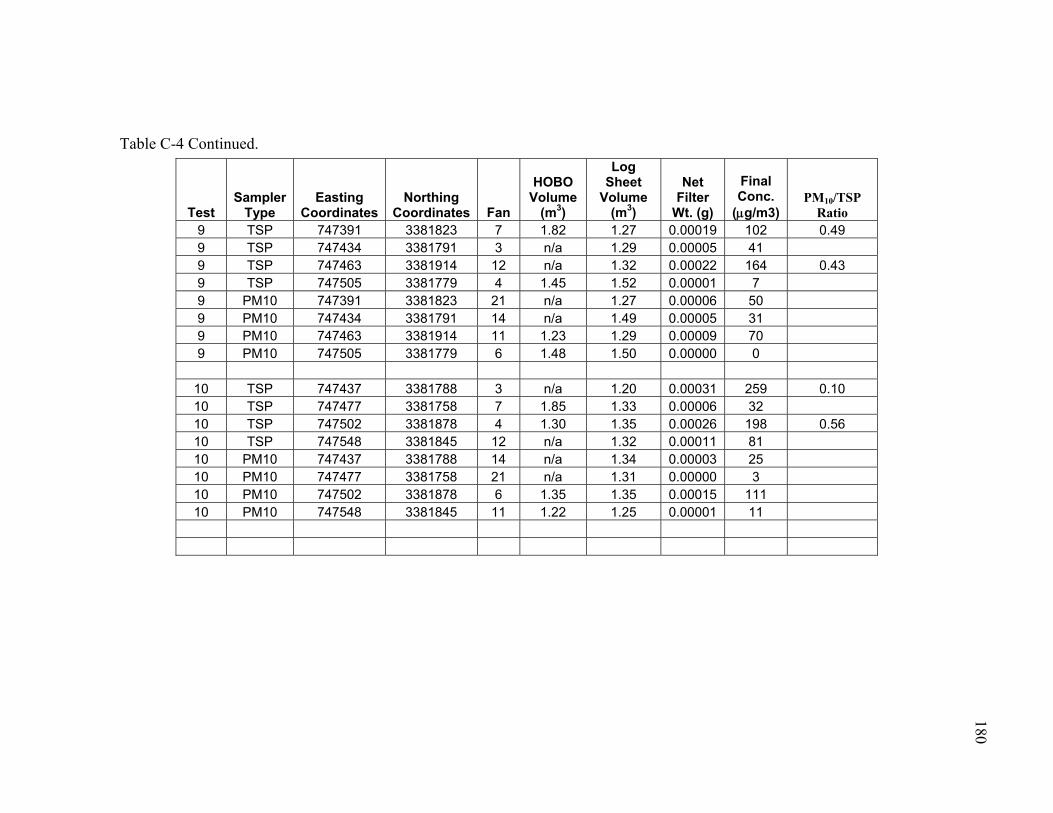
180
Table C-4 Continued.
Test Sampler
Type Easting
CoordinatesNorthing
Coordinates Fan
HOBO Volume
(m3)
Log Sheet
Volume (m3)
Net Filter
Wt. (g)
Final Conc.
(μg/m3)PM10/TSP
Ratio 9 TSP 747391 3381823 7 1.82 1.27 0.00019 102 0.49 9 TSP 747434 3381791 3 n/a 1.29 0.00005 41 9 TSP 747463 3381914 12 n/a 1.32 0.00022 164 0.43 9 TSP 747505 3381779 4 1.45 1.52 0.00001 7 9 PM10 747391 3381823 21 n/a 1.27 0.00006 50 9 PM10 747434 3381791 14 n/a 1.49 0.00005 31 9 PM10 747463 3381914 11 1.23 1.29 0.00009 70 9 PM10 747505 3381779 6 1.48 1.50 0.00000 0
10 TSP 747437 3381788 3 n/a 1.20 0.00031 259 0.10 10 TSP 747477 3381758 7 1.85 1.33 0.00006 32 10 TSP 747502 3381878 4 1.30 1.35 0.00026 198 0.56 10 TSP 747548 3381845 12 n/a 1.32 0.00011 81 10 PM10 747437 3381788 14 n/a 1.34 0.00003 25 10 PM10 747477 3381758 21 n/a 1.31 0.00000 3 10 PM10 747502 3381878 6 1.35 1.35 0.00015 111 10 PM10 747548 3381845 11 1.22 1.25 0.00001 11

181
Table C-4 Continued.
Test Sampler
Type Easting
CoordinatesNorthing
Coordinates Fan
HOBO Volume
(m3)
Log Sheet
Volume (m3)
Net Filter
Wt. (g)
Final Conc.
(μg/m3) PM10/TSP
Ratio 11 TSP 747555 3881675 3 n/a 0.97 0.00030 312 0.48 11 TSP 747594 3381637 7 1.33 0.92 0.00010 73 11 TSP 747610 3381745 4 1.13 0.94 0.00042 368 0.50 11 TSP 747646 3381707 12 n/a 1.00 0.00015 150 11 PM10 747555 3881675 14 n/a 1.06 0.00016 151 11 PM10 747594 3381637 21 n/a 0.93 0.00000 0 11 PM10 747610 3381745 6 0.92 0.92 0.00017 186 11 PM10 747646 3381707 11 0.96 0.99 0.00003 35
12 TSP 747592 3381635 7 1.78 1.26 0.00036 205 0.51 12 TSP 747629 3381595 3 n/a 0.84 0.00004 51 12 TSP 747646 3381703 12 n/a 1.15 0.00036 310 0.55 12 TSP 747684 3381662 4 1.19 1.04 0.00004 34 12 PM10 747592 3381635 21 n/a 1.24 0.00013 105 12 PM10 747629 3381595 14 n/a 0.88 0.00002 19 12 PM10 747646 3381703 11 1.08 1.12 0.00018 171 12 PM10 747684 3381662 6 1.00 1.02 0.00006 64
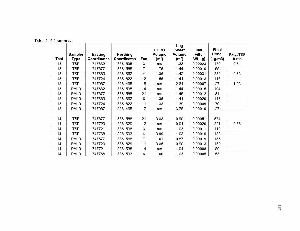
182
Table C-4 Continued.
Test Sampler
Type Easting
CoordinatesNorthing
Coordinates Fan
HOBO Volume
(m3)
Log Sheet
Volume (m3)
Net Filter
Wt. (g)
Final Conc.
(μg/m3)PM10/TSP
Ratio 13 TSP 747632 3381595 3 n/a 1.33 0.00023 170 0.61 13 TSP 747677 3381565 7 1.75 1.44 0.00010 55 13 TSP 747683 3381662 4 1.36 1.42 0.00031 230 0.63 13 TSP 747724 3381622 12 1.55 1.41 0.00018 116 13 TSP 747987 3381465 15 n/a 2.64 0.00007 27 1.03 13 PM10 747632 3381595 14 n/a 1.44 0.00015 104 13 PM10 747677 3381565 21 n/a 1.45 0.00012 81 13 PM10 747683 3381662 6 1.35 1.41 0.00020 146 13 PM10 747724 3381622 11 1.33 1.39 0.00009 70 13 PM10 747987 3381465 17 n/a 3.78 0.00010 27
14 TSP 747677 3381568 21 0.88 0.90 0.00051 574 14 TSP 747720 3381629 12 n/a 0.91 0.00020 221 0.68 14 TSP 747721 3381538 3 n/a 1.03 0.00011 110 14 TSP 747768 3381593 4 0.99 1.03 0.00019 188 14 PM10 747677 3381568 7 1.01 0.87 0.00019 185 14 PM10 747720 3381629 11 0.85 0.90 0.00013 150 14 PM10 747721 3381538 14 n/a 1.04 0.00008 80 14 PM10 747768 3381593 6 1.00 1.03 0.00005 53

183
Table C-4 Continued.
Test Sampler
Type Easting
CoordinatesNorthing
Coordinates Fan
HOBO Volume
(m3)
Log Sheet
Volume (m3)
Net Filter
Wt. (g)
Final Conc.
(μg/m3) PM10/TSP
Ratio 15 TSP 747721 3381538 3 0.66 0.66 0.00008 116 0.85 15 TSP 747762 3381497 7 n/a 0.69 0.00004 53 15 TSP 747766 3381599 4 0.69 0.69 0.00030 431 0.34 15 TSP 747807 3381557 12 n/a 0.71 0.00002 28 15 PM10 747721 3381538 14 n/a 0.74 0.00007 99 15 PM10 747762 3381497 21 0.67 0.68 0.00003 40 15 PM10 747766 3381599 6 0.68 0.70 0.00010 146 15 PM10 747807 3381557 11 0.67 0.75 0.00001 10
16 TSP 747625 3381504 15 n/a 1.74 0.00007 38 0.89 16 TSP 747906 3381313 3 n/a 1.84 0.00050 272 0.34 16 TSP 747950 3381328 12 2.41 2.05 0.00003 14 16 TSP 748014 3381246 4 1.77 1.84 0.00050 282 0.32 16 TSP 748052 3381264 7 n/a 2.07 0.00011 55 16 PM10 747625 3381504 17 2.27 2.35 0.00008 34 16 PM10 747906 3381313 14 n/a 2.10 0.00020 94 16 PM10 747950 3381328 11 2.37 2.02 0.00006 27 16 PM10 748014 3381246 6 1.77 1.83 0.00016 90 16 PM10 748052 3381264 21 n/a 2.04 0.00004 18
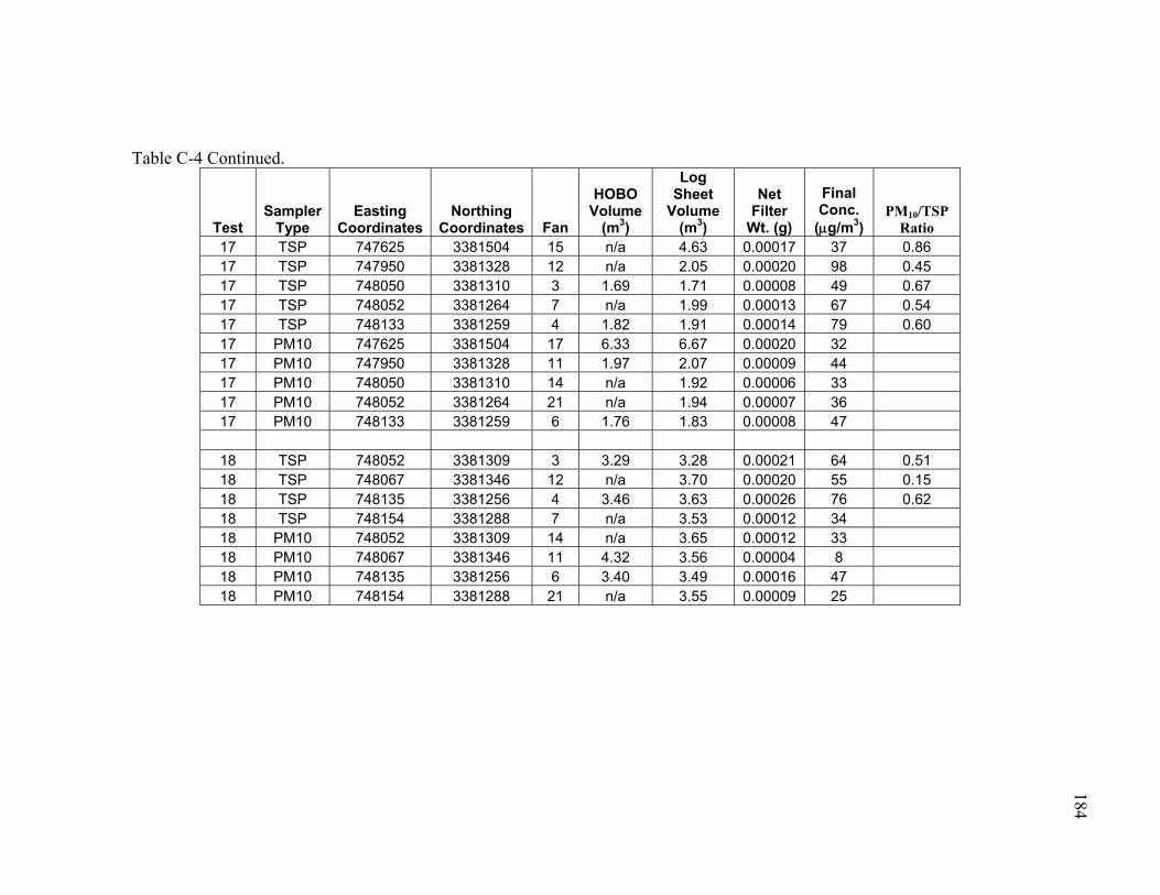
184
Table C-4 Continued.
Test Sampler
Type Easting
CoordinatesNorthing
Coordinates Fan
HOBO Volume
(m3)
Log Sheet
Volume (m3)
Net Filter
Wt. (g)
Final Conc.
(μg/m3) PM10/TSP
Ratio 17 TSP 747625 3381504 15 n/a 4.63 0.00017 37 0.86 17 TSP 747950 3381328 12 n/a 2.05 0.00020 98 0.45 17 TSP 748050 3381310 3 1.69 1.71 0.00008 49 0.67 17 TSP 748052 3381264 7 n/a 1.99 0.00013 67 0.54 17 TSP 748133 3381259 4 1.82 1.91 0.00014 79 0.60 17 PM10 747625 3381504 17 6.33 6.67 0.00020 32 17 PM10 747950 3381328 11 1.97 2.07 0.00009 44 17 PM10 748050 3381310 14 n/a 1.92 0.00006 33 17 PM10 748052 3381264 21 n/a 1.94 0.00007 36 17 PM10 748133 3381259 6 1.76 1.83 0.00008 47
18 TSP 748052 3381309 3 3.29 3.28 0.00021 64 0.51 18 TSP 748067 3381346 12 n/a 3.70 0.00020 55 0.15 18 TSP 748135 3381256 4 3.46 3.63 0.00026 76 0.62 18 TSP 748154 3381288 7 n/a 3.53 0.00012 34 18 PM10 748052 3381309 14 n/a 3.65 0.00012 33 18 PM10 748067 3381346 11 4.32 3.56 0.00004 8 18 PM10 748135 3381256 6 3.40 3.49 0.00016 47 18 PM10 748154 3381288 21 n/a 3.55 0.00009 25
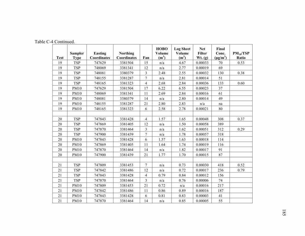
185
Table C-4 Continued.
Test Sampler
Type Easting
Coordinates Northing
Coordinates Fan
HOBO Volume
(m3)
Log Sheet Volume
(m3)
Net Filter
Wt. (g)
Final Conc.
(μg/m3) PM10/TSP
Ratio 19 TSP 747629 3381504 15 n/a 4.67 0.00033 70 0.53 19 TSP 748069 3381341 12 n/a 2.77 0.00019 69 19 TSP 748081 3380379 3 2.48 2.55 0.00032 130 0.38 19 TSP 748155 3381287 7 n/a 2.81 0.00014 51 19 TSP 748165 3381323 4 2.68 2.84 0.00036 133 0.60 19 PM10 747629 3381504 17 6.22 6.55 0.00023 37 19 PM10 748069 3381341 11 2.69 2.84 0.00016 61 19 PM10 748081 3380379 14 n/a 2.80 0.00014 49 19 PM10 748155 3381287 21 2.80 2.83 n/a na 19 PM10 748165 3381323 6 2.58 2.78 0.00021 80
20 TSP 747843 3381428 4 1.57 1.65 0.00048 308 0.37 20 TSP 747869 3381405 12 n/a 1.50 0.00058 389 20 TSP 747870 3381464 3 n/a 1.62 0.00051 312 0.29 20 TSP 747900 3381439 7 n/a 1.78 0.00057 318 20 PM10 747843 3381428 6 1.57 1.63 0.00018 114 20 PM10 747869 3381405 11 1.64 1.74 0.00019 116 20 PM10 747870 3381464 14 n/a 1.82 0.00017 91 20 PM10 747900 3381439 21 1.77 1.70 0.00015 87
21 TSP 747809 3381453 7 n/a 0.73 0.00030 418 0.52 21 TSP 747842 3381486 12 n/a 0.72 0.00017 236 0.79 21 TSP 747843 3381428 4 0.79 0.84 0.00012 156 21 TSP 747870 3381464 3 n/a 0.76 0.00006 74 21 PM10 747809 3381453 21 0.72 n/a 0.00016 217 21 PM10 747842 3381486 11 0.86 0.89 0.00016 187 21 PM10 747843 3381428 6 0.81 0.83 0.00003 41 21 PM10 747870 3381464 14 n/a 0.85 0.00005 55

186
APPENDIX D
SYSTEMATIC UNCERTAINTY ANALYSIS FOR THE SOURCE SAMPLING
SYSTEM

187
Table D-1. Manufacturer published uncertainty values for the components used in the source sampling system used onboard the six-row cotton picker.
Variable Description Instrument Reported Uncertainty Source
MF1 Initial Mass of Filter Bank Filters
Metler Toledo XS205 Balance 2*10-4 g MT Manual
MF2 Final Mass of Filter Bank Filters
Metler Toledo XS205 Balance 2*10-4 g MT Manual
MC1 Initial Mass of Cyclone Bucket Filter
Metler Toledo XS205 Balance 2*10-4 g MT Manual
MC2 Final Mass of Cyclone Bucket Filter
Metler Toledo XS205 Balance 2*10-4 g MT Manual
QLFE Mass Flow Controller Flow Rate
Meriam Laminar Flow Element Model 50MC2-2 0.86% of reading Meriam Manual
Do Orifice Diameter Orifice Meter (shop made) 0.001 Mitutoyo Caliper Manual
∆Pc Calibration pressure drop Dwyer Series 475 Mark III Digital Manometer
0.5% Full Scale (0.1 in H2O) Specification Sheet
Patm,c Calibration Ambient Pressure
Davis Perception II 1.3 mm Hg Specification Sheet
φc Calibration Ambient Relative Humidity Ratio
Davis Perception II 5% Specification Sheet
Ps,c Calibration Saturation Pressure
Steam Table 0.0001 psia Specification Sheet
Tc Calibration Ambient Temp
Davis Perception II 1°F Specification Sheet
∆Ps Sample Orifice Meter Pressure Drop
Dwyer 677 Pressure Transducer (range: 0 - 2.5 in H2O, Accuracy: 0.4 %FS) + National Instruments cFP-AI-110 (0.016 %FS)
0.0104 in H2O Specification Sheet
Patm,s Sampling Ambient Pressure
Setra Model 278 Barometric Pressure Transmitter (0.5 hPa) + National Instruments cFP-AI-110 (0.016 %FS)
0.009804 psia Specification Sheet

188
Table D-1 Continued.
Variable Description Instrument Reported Uncertainty Source
φ Sampling Ambient Relative Humidity Ratio
Omega HX94A T/RH Probe (3.1 %) + National Instruments cFP-AI-110 (0.016 %FS)
0.00310 Specification Sheet
Ps Saturation Pressure Steam Table 0.0001 psia Specification Sheet
T Temperature during sampling
Omega HX94A T/RH Probe (1 degree F) + National Instruments cFP-AI-110 (0.016 %FS)
1.03392 F Specification Sheet
t Elapsed Time Dell Laptop Computer - Latitude D820 0.00001 min/min assumed
VP Duct Velocity Pressure Dwyer 677 Pressure Transducer (range: 0 - 1.0 in H2O, Accuracy: 0.4 %FS) + National Instruments cFP-AI-110 (0.016 %FS)
0.00416 in H2O Specification Sheet
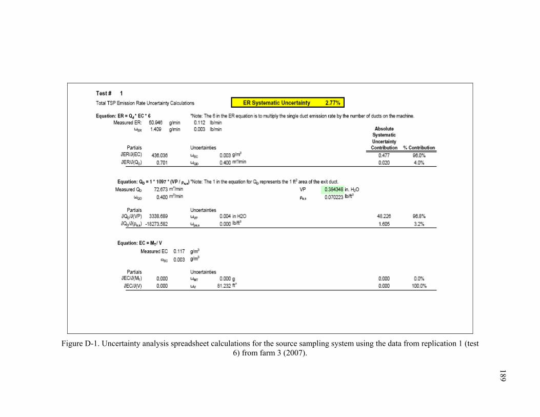
189
Figure D-1. Uncertainty analysis spreadsheet calculations for the source sampling system using the data from replication 1 (test
6) from farm 3 (2007).

190
Figure D-1 Continued.

191
Figure D-1 Continued.

192
APPENDIX E
ASH ANALYSIS RESULTS FOR PARTICULATE MATTER LESS THAN 100
MICROMETERS CAPTURED IN THE SOURCE SAMPLER CYCLONE
BUCKET

193
Ash analysis of the PM<100 μm captured in the source sampler cyclone bucket
was conducted to give insight as to the primary constituents which make up the captured
material. The Standard Test Method for Ash in Biomass (ASTM, 2001) was used to
perform the analysis. Wanjura et al. (2006) indicated through the results of ash analyses
that the primary constituent in the material air washed from seed cotton samples is soil.
Thus, it was expected that the primary constituent in the PM <100 μm air washed from
the material captured in the cyclone bucket would also be primarily comprised of soil.
However, the results of the analysis indicate that the average ash content of the samples
was 25.35%. This result is likely a consequence of increased portions of volatile
material such as plant material and lint fiber captured by the cyclone. The results of the
ash analysis are presented in Table E-1.
Table E-1. Ash analysis results for the PM <100μm captured in the source sampler cyclone bucket.
Test Ash Content
(%) 1 28.2 2 26.4 3 27.2 4 25.5 5 24.6 6 23.7 7 21.5 8 21.9 9 25.8
10 28.7
Mean Ash % 25.4 95% C.I. 1.5

194
References:
ASTM Standards. 2001. E1755-01: Standard test method for ash in biomass. West Conshohocken, PA.: ASTM International.
Wanjura, J.D., C.B. Parnell, Jr., B.W. Shaw, and S.C. Capareda. 2006. Particle size
distribution of PM emitted from cotton harvesting. ASABE Paper No. 064168. St. Joseph, Mich.: ASABE.

195
APPENDIX F
TEST SUMMARY SHEETS FOR THE SOURCE SAMPLING TESTS
CONDUCTED DURING 2007
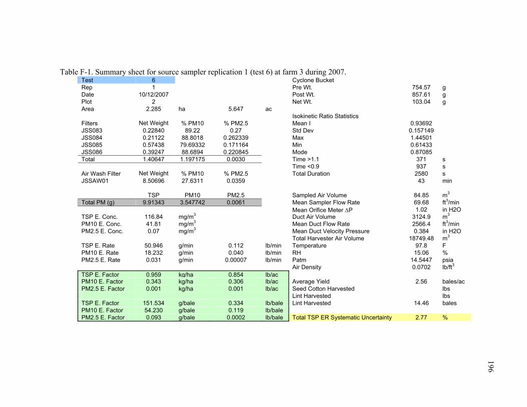
196
Table F-1. Summary sheet for source sampler replication 1 (test 6) at farm 3 during 2007. Test 6 Cyclone Bucket Rep 1 Pre Wt. 754.57 g Date 10/12/2007 Post Wt. 857.61 g Plot 2 Net Wt. 103.04 g Area 2.285 ha 5.647 ac Isokinetic Ratio Statistics Filters Net Weight % PM10 % PM2.5 Mean I 0.93692 JSS083 0.22840 89.22 0.27 Std Dev 0.157149 JSS084 0.21122 88.8018 0.262339 Max 1.44501 JSS085 0.57438 79.69332 0.171164 Min 0.61433 JSS086 0.39247 88.6894 0.220845 Mode 0.87085 Total 1.40647 1.197175 0.0030 Time >1.1 371 s Time <0.9 937 s Air Wash Filter Net Weight % PM10 % PM2.5 Total Duration 2580 s JSSAW01 8.50696 27.6311 0.0359 43 min TSP PM10 PM2.5 Sampled Air Volume 84.85 m3 Total PM (g) 9.91343 3.547742 0.0061 Mean Sampler Flow Rate 69.68 ft3/min Mean Orifice Meter ΔP 1.02 in H2O TSP E. Conc. 116.84 mg/m3 Duct Air Volume 3124.9 m3 PM10 E. Conc. 41.81 mg/m3 Mean Duct Flow Rate 2566.4 ft3/min PM2.5 E. Conc. 0.07 mg/m3 Mean Duct Velocity Pressure 0.384 in H2O Total Harvester Air Volume 18749.48 m3 TSP E. Rate 50.946 g/min 0.112 lb/min Temperature 97.8 F PM10 E. Rate 18.232 g/min 0.040 lb/min RH 15.06 % PM2.5 E. Rate 0.031 g/min 0.00007 lb/min Patm 14.5447 psia Air Density 0.0702 lb/ft3 TSP E. Factor 0.959 kg/ha 0.854 lb/acPM10 E. Factor 0.343 kg/ha 0.306 lb/ac Average Yield 2.56 bales/ac PM2.5 E. Factor 0.001 kg/ha 0.001 lb/ac Seed Cotton Harvested lbs Lint Harvested lbs TSP E. Factor 151.534 g/bale 0.334 lb/bale Lint Harvested 14.46 bales PM10 E. Factor 54.230 g/bale 0.119 lb/bale PM2.5 E. Factor 0.093 g/bale 0.0002 lb/bale Total TSP ER Systematic Uncertainty 2.77 %

197
Table F-2. Summary sheet for source sampler replication 2 (test 7) at farm 3 during 2007. Test 7 Cyclone Bucket Rep 2 Pre Wt. 754.71 g Date 10/12/2007 Post Wt. 850.59 g Plot 3 Net Wt. 95.88 g Area 2.064 ha 5.100 ac Isokinetic Ratio Statistics Filters Net Weight (g) % PM10 % PM2.5 Mean I 0.963579 JSS119 0.27327 91.1359 0.240331 Std Dev 0.126655 JSS120 0.34198 87.12484 0.206943 Max 1.8939 JSS121 0.30647 90.1381 0.208826 Min 0.66698 JSS122 0.30331 88.8907 0.147423 Mode 0.86453 Total 1.22502 1.092851 0.0025 Time >1.1 307 s Time <0.9 688 s Air Wash Filter Net Weight (g) % PM10 % PM2.5 Total Duration 2543 s JSSAW02 7.32133 27.789 0.0400 42.38333 min TSP PM10 PM2.5 Sampled Air Volume 76.96 m3 Total PM (g) 8.54636 3.127376 0.0054 Mean Sampler Flow Rate 64.13 ft3/min Mean Orifice Meter ΔP 0.88 in H2O TSP E. Conc. 111.04 mg/m3 Duct Air Volume 2754.1 m3 PM10 E. Conc. 40.63 mg/m3 Mean Duct Flow Rate 2294.8 ft3/min PM2.5 E. Conc. 0.07 mg/m3 Mean Duct Velocity Pressure 0.313 in H2O Total Harvester Air Volume 16524.32 m3 TSP E. Rate 43.293 g/min 0.095 lb/min Temperature 87.4 F PM10 E. Rate 15.842 g/min 0.035 lb/min RH 26.23 % PM2.5 E. Rate 0.027 g/min 0.00006 lb/min Patm 14.5434 psia Air Density 0.0715 lb/ft3 TSP E. Factor 0.889 kg/ha 0.792 lb/ac PM10 E. Factor 0.325 kg/ha 0.290 lb/ac Average Yield 2.41 bales/ac PM2.5 E. Factor 0.001 kg/ha 0.000 lb/ac Seed Cotton Harvested lbs Lint Harvested lbs TSP E. Factor 149.286 g/bale 0.329 lb/bale Lint Harvested 12.29 bales PM10 E. Factor 54.628 g/bale 0.120 lb/bale PM2.5 E. Factor 0.094 g/bale 0.0002 lb/bale Total ER Systematic Uncertainty 2.81 %

198
Table F-3. Summary sheet for source sampler replication 3 (test 8) at farm 3 during 2007. Test 8 Cyclone Bucket Rep 3 Pre Wt. 754.1 g Date 10/13/2007 Post Wt. 804.6 g Plot 5 Net Wt. 50.5 g Area 1.251 ha 3.092 ac Isokinetic Ratio Statistics Filters Net Weight (g) % PM10 % PM2.5 Mean I 0.982389 JSS115 0.16510 90.59216 0.213783 Std Dev 0.08747 JSS116 0.16704 91.75049 0.242711 Max 1.26099 JSS117 0.29273 91.94145 0.233275 Min 0.75254 JSS118 0.31108 92.94763 0.229939 Mode 1.11926 Total 0.93595 0.861112 0.0022 Time >1.1 140 s Time <0.9 247 s Air Wash Filter Net Weight (g) % PM10 % PM2.5 Total Duration 1638 s JSSAW03 4.89988 24.7823 0.0441 27.3 min TSP PM10 PM2.5 Sampled Air Volume 54.24 m3 Total PM (g) 5.83583 2.075415 0.0043 Mean Sampler Flow Rate 70.17 ft3/min Mean Orifice Meter ΔP 1.05 in H2O TSP E. Conc. 107.58 mg/m3 Duct Air Volume 1887.6 m3 PM10 E. Conc. 38.26 mg/m3 Mean Duct Flow Rate 2441.7 ft3/min PM2.5 E. Conc. 0.08 mg/m3 Mean Duct Velocity Pressure 0.353 in H2O Total Harvester Air Volume 11325.4 m3 TSP E. Rate 44.631 g/min 0.098 lb/min Temperature 90.6 F PM10 E. Rate 15.872 g/min 0.035 lb/min RH 20.91 % PM2.5 E. Rate 0.033 g/min 0.00007 lb/min Patm 14.5655 psia Air Density 0.0712 lb/ft3 TSP E. Factor 0.974 kg/ha 0.868 lb/ac PM10 E. Factor 0.346 kg/ha 0.309 lb/ac Average Yield 2.396 bales/ac PM2.5 E. Factor 0.001 kg/ha 0.001 lb/ac Seed Cotton Harvested lbs Lint Harvested lbs TSP E. Factor 164.489 g/bale 0.362 lb/bale Lint Harvested 7.41 bales PM10 E. Factor 58.498 g/bale 0.129 lb/bale PM2.5 E. Factor 0.122 g/bale 0.0003 lb/bale Total ER Systematic Uncertainty 2.77 %
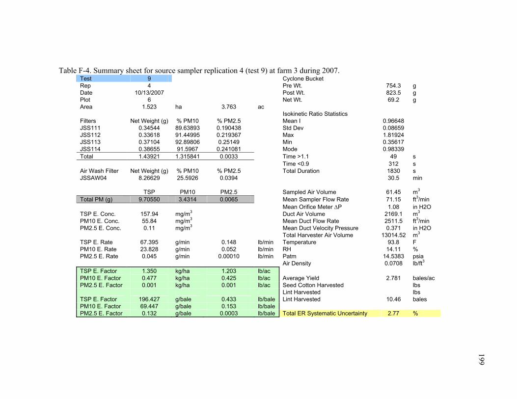
199
Table F-4. Summary sheet for source sampler replication 4 (test 9) at farm 3 during 2007. Test 9 Cyclone Bucket Rep 4 Pre Wt. 754.3 g Date 10/13/2007 Post Wt. 823.5 g Plot 6 Net Wt. 69.2 g Area 1.523 ha 3.763 ac Isokinetic Ratio Statistics Filters Net Weight (g) % PM10 % PM2.5 Mean I 0.96648 JSS111 0.34544 89.63893 0.190438 Std Dev 0.08659 JSS112 0.33618 91.44995 0.219367 Max 1.81924 JSS113 0.37104 92.89806 0.25149 Min 0.35617 JSS114 0.38655 91.5967 0.241081 Mode 0.98339 Total 1.43921 1.315841 0.0033 Time >1.1 49 s Time <0.9 312 s Air Wash Filter Net Weight (g) % PM10 % PM2.5 Total Duration 1830 s JSSAW04 8.26629 25.5926 0.0394 30.5 min TSP PM10 PM2.5 Sampled Air Volume 61.45 m3 Total PM (g) 9.70550 3.4314 0.0065 Mean Sampler Flow Rate 71.15 ft3/min Mean Orifice Meter ΔP 1.08 in H2O TSP E. Conc. 157.94 mg/m3 Duct Air Volume 2169.1 m3 PM10 E. Conc. 55.84 mg/m3 Mean Duct Flow Rate 2511.5 ft3/min PM2.5 E. Conc. 0.11 mg/m3 Mean Duct Velocity Pressure 0.371 in H2O Total Harvester Air Volume 13014.52 m3 TSP E. Rate 67.395 g/min 0.148 lb/min Temperature 93.8 F PM10 E. Rate 23.828 g/min 0.052 lb/min RH 14.11 % PM2.5 E. Rate 0.045 g/min 0.00010 lb/min Patm 14.5383 psia Air Density 0.0708 lb/ft3 TSP E. Factor 1.350 kg/ha 1.203 lb/ac PM10 E. Factor 0.477 kg/ha 0.425 lb/ac Average Yield 2.781 bales/ac PM2.5 E. Factor 0.001 kg/ha 0.001 lb/ac Seed Cotton Harvested lbs Lint Harvested lbs TSP E. Factor 196.427 g/bale 0.433 lb/bale Lint Harvested 10.46 bales PM10 E. Factor 69.447 g/bale 0.153 lb/bale PM2.5 E. Factor 0.132 g/bale 0.0003 lb/bale Total ER Systematic Uncertainty 2.77 %
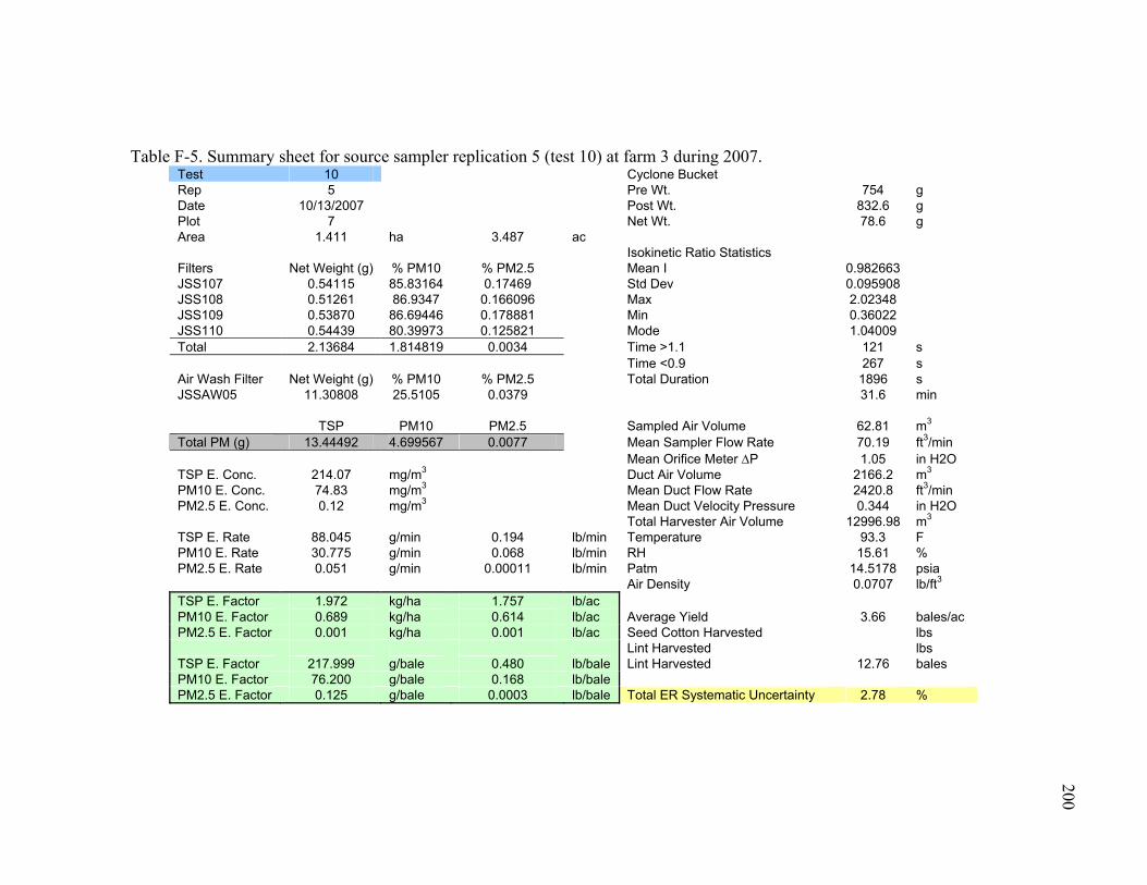
200
Table F-5. Summary sheet for source sampler replication 5 (test 10) at farm 3 during 2007. Test 10 Cyclone Bucket Rep 5 Pre Wt. 754 g Date 10/13/2007 Post Wt. 832.6 g Plot 7 Net Wt. 78.6 g Area 1.411 ha 3.487 ac Isokinetic Ratio Statistics Filters Net Weight (g) % PM10 % PM2.5 Mean I 0.982663 JSS107 0.54115 85.83164 0.17469 Std Dev 0.095908 JSS108 0.51261 86.9347 0.166096 Max 2.02348 JSS109 0.53870 86.69446 0.178881 Min 0.36022 JSS110 0.54439 80.39973 0.125821 Mode 1.04009 Total 2.13684 1.814819 0.0034 Time >1.1 121 s Time <0.9 267 s Air Wash Filter Net Weight (g) % PM10 % PM2.5 Total Duration 1896 s JSSAW05 11.30808 25.5105 0.0379 31.6 min TSP PM10 PM2.5 Sampled Air Volume 62.81 m3 Total PM (g) 13.44492 4.699567 0.0077 Mean Sampler Flow Rate 70.19 ft3/min Mean Orifice Meter ΔP 1.05 in H2O TSP E. Conc. 214.07 mg/m3 Duct Air Volume 2166.2 m3 PM10 E. Conc. 74.83 mg/m3 Mean Duct Flow Rate 2420.8 ft3/min PM2.5 E. Conc. 0.12 mg/m3 Mean Duct Velocity Pressure 0.344 in H2O Total Harvester Air Volume 12996.98 m3 TSP E. Rate 88.045 g/min 0.194 lb/min Temperature 93.3 F PM10 E. Rate 30.775 g/min 0.068 lb/min RH 15.61 % PM2.5 E. Rate 0.051 g/min 0.00011 lb/min Patm 14.5178 psia Air Density 0.0707 lb/ft3 TSP E. Factor 1.972 kg/ha 1.757 lb/ac PM10 E. Factor 0.689 kg/ha 0.614 lb/ac Average Yield 3.66 bales/ac PM2.5 E. Factor 0.001 kg/ha 0.001 lb/ac Seed Cotton Harvested lbs Lint Harvested lbs TSP E. Factor 217.999 g/bale 0.480 lb/bale Lint Harvested 12.76 bales PM10 E. Factor 76.200 g/bale 0.168 lb/bale PM2.5 E. Factor 0.125 g/bale 0.0003 lb/bale Total ER Systematic Uncertainty 2.78 %

201
Table F-6. Summary sheet for source sampler replication 6 (test 11) at farm 3 during 2007. Test 11 Cyclone Bucket Rep 6 Pre Wt. 754.1 g Date 10/13/2007 Post Wt. 813.7 g Plot 10 Net Wt. 59.6 g Area 1.232 ha 3.045 ac Isokinetic Ratio Statistics Filters Net Weight (g) % PM10 % PM2.5 Mean I 0.904214 JSS103 0.47415 89.28906 0.235751 Std Dev 0.116078 JSS104 0.51428 85.94582 0.217005 Max 1.24404 JSS105 0.20530 85.83048 0.174416 Min 0.57405 JSS106 0.20768 85.53245 0.20493 Mode 0.98755 Total 1.40141 1.219213 0.0030 Time >1.1 37 s Time <0.9 700 s Air Wash Filter Net Weight (g) % PM10 % PM2.5 Total Duration 1640 s JSSAW06 8.75216 26.5354 0.0349 27.33333 min TSP PM10 PM2.5 Sampled Air Volume 51.32 m3 Total PM (g) 10.15357 3.541633 0.0061 Mean Sampler Flow Rate 66.30 ft3/min Mean Orifice Meter ΔP 0.94 in H2O TSP E. Conc. 197.86 mg/m3 Duct Air Volume 1970.3 m3 PM10 E. Conc. 69.02 mg/m3 Mean Duct Flow Rate 2545.7 ft3/min PM2.5 E. Conc. 0.12 mg/m3 Mean Duct Velocity Pressure 0.383 in H2O Total Harvester Air Volume 11821.8 m3 TSP E. Rate 85.577 g/min 0.188 lb/min Temperature 89.7 F PM10 E. Rate 29.850 g/min 0.066 lb/min RH 20.03 % PM2.5 E. Rate 0.051 g/min 0.00011 lb/min Patm 14.5098 psia Air Density 0.0711 lb/ft3 TSP E. Factor 1.898 kg/ha 1.692 lb/ac PM10 E. Factor 0.662 kg/ha 0.590 lb/ac Average Yield 3.75 bales/ac PM2.5 E. Factor 0.001 kg/ha 0.001 lb/ac Seed Cotton Harvested lbs Lint Harvested lbs TSP E. Factor 204.875 g/bale 0.451 lb/bale Lint Harvested 11.42 bales PM10 E. Factor 71.462 g/bale 0.157 lb/bale PM2.5 E. Factor 0.123 g/bale 0.0003 lb/bale Total ER Systematic Uncertainty 2.78 %
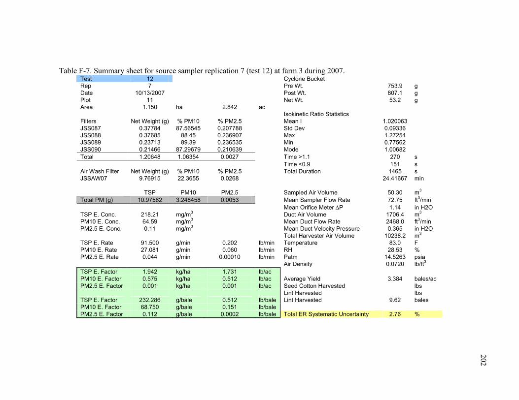
202
Table F-7. Summary sheet for source sampler replication 7 (test 12) at farm 3 during 2007. Test 12 Cyclone Bucket Rep 7 Pre Wt. 753.9 g Date 10/13/2007 Post Wt. 807.1 g Plot 11 Net Wt. 53.2 g Area 1.150 ha 2.842 ac Isokinetic Ratio Statistics Filters Net Weight (g) % PM10 % PM2.5 Mean I 1.020063 JSS087 0.37784 87.56545 0.207788 Std Dev 0.09336 JSS088 0.37685 88.45 0.236907 Max 1.27254 JSS089 0.23713 89.39 0.236535 Min 0.77562 JSS090 0.21466 87.29679 0.210639 Mode 1.00682 Total 1.20648 1.06354 0.0027 Time >1.1 270 s Time <0.9 151 s Air Wash Filter Net Weight (g) % PM10 % PM2.5 Total Duration 1465 s JSSAW07 9.76915 22.3655 0.0268 24.41667 min TSP PM10 PM2.5 Sampled Air Volume 50.30 m3 Total PM (g) 10.97562 3.248458 0.0053 Mean Sampler Flow Rate 72.75 ft3/min Mean Orifice Meter ΔP 1.14 in H2O TSP E. Conc. 218.21 mg/m3 Duct Air Volume 1706.4 m3 PM10 E. Conc. 64.59 mg/m3 Mean Duct Flow Rate 2468.0 ft3/min PM2.5 E. Conc. 0.11 mg/m3 Mean Duct Velocity Pressure 0.365 in H2O Total Harvester Air Volume 10238.2 m3 TSP E. Rate 91.500 g/min 0.202 lb/min Temperature 83.0 F PM10 E. Rate 27.081 g/min 0.060 lb/min RH 28.53 % PM2.5 E. Rate 0.044 g/min 0.00010 lb/min Patm 14.5263 psia Air Density 0.0720 lb/ft3 TSP E. Factor 1.942 kg/ha 1.731 lb/ac PM10 E. Factor 0.575 kg/ha 0.512 lb/ac Average Yield 3.384 bales/ac PM2.5 E. Factor 0.001 kg/ha 0.001 lb/ac Seed Cotton Harvested lbs Lint Harvested lbs TSP E. Factor 232.286 g/bale 0.512 lb/bale Lint Harvested 9.62 bales PM10 E. Factor 68.750 g/bale 0.151 lb/bale PM2.5 E. Factor 0.112 g/bale 0.0002 lb/bale Total ER Systematic Uncertainty 2.76 %

203
Table F-8. Summary sheet for source sampler replication 8 (test 13) at farm 3 during 2007. Test 13 Cyclone Bucket Rep 8 Pre Wt. 754.3 g Date 10/14/2007 Post Wt. 790.5 g Plot 12 Net Wt. 36.2 g Area 1.073 ha 2.652 ac Isokinetic Ratio Statistics Filters Net Weight (g) % PM10 % PM2.5 Mean I 0.923153 JSS091 0.31577 77.04225 0.128076 Std Dev 0.095159 JSS092 0.41133 78.11227 0.118964 Max 1.26909 JSS093 0.18200 89.32967 0.250577 Min 0.69133 JSS094 0.20352 92.18332 0.254697 Mode 1.14645 Total 1.11262 0.91477 0.0019 Time >1.1 65 s Time <0.9 472 s Air Wash Filter Net Weight (g) % PM10 % PM2.5 Total Duration 1308 s JSSAW08 5.35671 21.7653 0.0331 21.8 min TSP PM10 PM2.5 Sampled Air Volume 41.51 m3 Total PM (g) 6.46933 2.080673 0.0036 Mean Sampler Flow Rate 67.24 ft3/min Mean Orifice Meter ΔP 0.96 in H2O TSP E. Conc. 155.86 mg/m3 Duct Air Volume 1557.7 m3 PM10 E. Conc. 50.13 mg/m3 Mean Duct Flow Rate 2523.3 ft3/min PM2.5 E. Conc. 0.09 mg/m3 Mean Duct Velocity Pressure 0.375 in H2O Total Harvester Air Volume 9345.97 m3 TSP E. Rate 66.818 g/min 0.147 lb/min Temperature 89.8 F PM10 E. Rate 21.490 g/min 0.047 lb/min RH 31.72 % PM2.5 E. Rate 0.038 g/min 0.00008 lb/min Patm 14.5054 psia Air Density 0.0709 lb/ft3 TSP E. Factor 1.357 kg/ha 1.210 lb/ac PM10 E. Factor 0.436 kg/ha 0.389 lb/ac Average Yield 3.319 bales/ac PM2.5 E. Factor 0.001 kg/ha 0.001 lb/ac Seed Cotton Harvested lbs Lint Harvested lbs TSP E. Factor 165.471 g/bale 0.364 lb/bale Lint Harvested 8.80 bales PM10 E. Factor 53.219 g/bale 0.117 lb/bale PM2.5 E. Factor 0.093 g/bale 0.0002 lb/bale Total ER Systematic Uncertainty 2.78 %

204
Table F-9. Summary sheet for source sampler replication 9 (test 14) at farm 3 during 2007. Test 14 Cyclone Bucket Rep 9 Pre Wt. 754.4 g Date 10/14/2007 Post Wt. 793.4 g Plot 13 Net Wt. 39 g Area 1.013 ha 2.502 ac Isokinetic Ratio Statistics Filters Net Weight (g) % PM10 % PM2.5 Mean I 0.966917 JSS095 0.17838 83.80626 0.237139 Std Dev 0.066255 JSS096 0.16188 88.91568 0.284062 Max 1.1361 JSS097 0.21026 88.12787 0.308868 Min 0.77863 JSS098 0.21795 84.35546 0.215507 Mode 0.97821 Total 0.76846 0.662572 0.0020 Time >1.1 11 s Time <0.9 204 s Air Wash Filter Net Weight (g) % PM10 % PM2.5 Total Duration 1231 s JSSAW09 6.43266 29.7669 0.0427 20.51667 min TSP PM10 PM2.5 Sampled Air Volume 41.40 m3 Total PM (g) 7.20112 2.577375 0.0048 Mean Sampler Flow Rate 71.26 ft3/min Mean Orifice Meter ΔP 1.08 in H2O TSP E. Conc. 173.94 mg/m3 Duct Air Volume 1475.2 m3 PM10 E. Conc. 62.26 mg/m3 Mean Duct Flow Rate 2539.2 ft3/min PM2.5 E. Conc. 0.11 mg/m3 Mean Duct Velocity Pressure 0.380 in H2O Total Harvester Air Volume 8851.085 m3 TSP E. Rate 75.039 g/min 0.165 lb/min Temperature 89.5 F PM10 E. Rate 26.857 g/min 0.059 lb/min RH 33.47 % PM2.5 E. Rate 0.050 g/min 0.00011 lb/min Patm 14.4944 psia Air Density 0.0709 lb/ft3 TSP E. Factor 1.521 kg/ha 1.355 lb/ac PM10 E. Factor 0.544 kg/ha 0.485 lb/ac Average Yield 2.713 bales/ac PM2.5 E. Factor 0.001 kg/ha 0.001 lb/ac Seed Cotton Harvested lbs Lint Harvested lbs TSP E. Factor 226.812 g/bale 0.500 lb/bale Lint Harvested 6.79 bales PM10 E. Factor 81.179 g/bale 0.179 lb/bale PM2.5 E. Factor 0.150 g/bale 0.0003 lb/bale Total ER Systematic Uncertainty 2.76 %

205
Table F-10. Summary sheet for source sampler replication 10 (test 15) at farm 3 during 2007. Test 15 Cyclone Bucket Rep 10 Pre Wt. 754.5 g Date 10/14/2007 Post Wt. 788.8 g Plot 14 Net Wt. 34.3 g Area 1.013 ha 2.502 ac Isokinetic Ratio Statistics Filters Net Weight (g) % PM10 % PM2.5 Mean I 0.880302 JSS099 0.12973 89.35908 0.241746 Std Dev 0.124809 JSS100 0.13718 89.78184 0.237493 Max 1.17999 JSS101 0.16551 82.9302 0.223702 Min 0.60894 JSS102 0.15757 84.40168 0.221397 Mode 1.07194 Total 0.58999 0.509341 0.0014 Time >1.1 37 s Time <0.9 651 s Air Wash Filter Net Weight (g) % PM10 % PM2.5 Total Duration 1179 s JSSAW10 4.15692 21.4348 0.0468 19.65 min TSP PM10 PM2.5 Sampled Air Volume 35.37 m3 Total PM (g) 4.74691 1.400368 0.0033 Mean Sampler Flow Rate 63.57 ft3/min Mean Orifice Meter ΔP 0.86 in H2O TSP E. Conc. 134.21 mg/m3 Duct Air Volume 1407.3 m3 PM10 E. Conc. 39.59 mg/m3 Mean Duct Flow Rate 2529.2 ft3/min PM2.5 E. Conc. 0.09 mg/m3 Mean Duct Velocity Pressure 0.379 in H2O Total Harvester Air Volume 8443.729 m3 TSP E. Rate 57.669 g/min 0.127 lb/min Temperature 86.2 F PM10 E. Rate 17.013 g/min 0.037 lb/min RH 37.70 % PM2.5 E. Rate 0.040 g/min 0.00009 lb/min Patm 14.4936 psia Air Density 0.0713 lb/ft3 TSP E. Factor 1.119 kg/ha 0.997 lb/ac PM10 E. Factor 0.330 kg/ha 0.294 lb/ac Average Yield 3.055 bales/ac PM2.5 E. Factor 0.001 kg/ha 0.001 lb/ac Seed Cotton Harvested lbs Lint Harvested lbs TSP E. Factor 148.231 g/bale 0.327 lb/bale Lint Harvested 7.64 bales PM10 E. Factor 43.729 g/bale 0.096 lb/bale PM2.5 E. Factor 0.103 g/bale 0.0002 lb/bale Total ER Systematic Uncertainty 2.79 %

206
APPENDIX G
PARTICLE SIZE DISTRIBUTION RESULT STATISTICS FOR THE TSP
SAMPLER FILTERS AND PM CAPTURED BY THE SOURCE SAMPLER
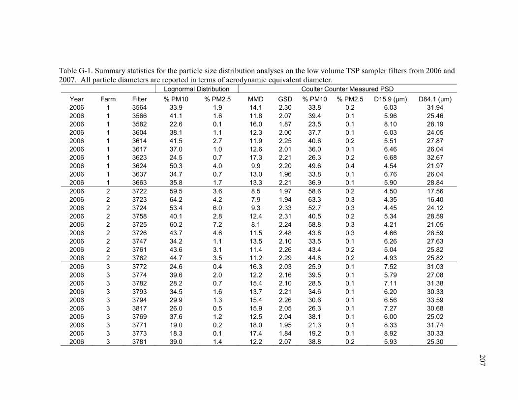
207
Table G-1. Summary statistics for the particle size distribution analyses on the low volume TSP sampler filters from 2006 and 2007. All particle diameters are reported in terms of aerodynamic equivalent diameter.
Lognormal Distribution Coulter Counter Measured PSD Year Farm Filter % PM10 % PM2.5 MMD GSD % PM10 % PM2.5 D15.9 (μm) D84.1 (μm) 2006 1 3564 33.9 1.9 14.1 2.30 33.8 0.2 6.03 31.94 2006 1 3566 41.1 1.6 11.8 2.07 39.4 0.1 5.96 25.46 2006 1 3582 22.6 0.1 16.0 1.87 23.5 0.1 8.10 28.19 2006 1 3604 38.1 1.1 12.3 2.00 37.7 0.1 6.03 24.05 2006 1 3614 41.5 2.7 11.9 2.25 40.6 0.2 5.51 27.87 2006 1 3617 37.0 1.0 12.6 2.01 36.0 0.1 6.46 26.04 2006 1 3623 24.5 0.7 17.3 2.21 26.3 0.2 6.68 32.67 2006 1 3624 50.3 4.0 9.9 2.20 49.6 0.4 4.54 21.97 2006 1 3637 34.7 0.7 13.0 1.96 33.8 0.1 6.76 26.04 2006 1 3663 35.8 1.7 13.3 2.21 36.9 0.1 5.90 28.84 2006 2 3722 59.5 3.6 8.5 1.97 58.6 0.2 4.50 17.56 2006 2 3723 64.2 4.2 7.9 1.94 63.3 0.3 4.35 16.40 2006 2 3724 53.4 6.0 9.3 2.33 52.7 0.3 4.45 24.12 2006 2 3758 40.1 2.8 12.4 2.31 40.5 0.2 5.34 28.59 2006 2 3725 60.2 7.2 8.1 2.24 58.8 0.3 4.21 21.05 2006 2 3726 43.7 4.6 11.5 2.48 43.8 0.3 4.66 28.59 2006 2 3747 34.2 1.1 13.5 2.10 33.5 0.1 6.26 27.63 2006 2 3761 43.6 3.1 11.4 2.26 43.4 0.2 5.04 25.82 2006 2 3762 44.7 3.5 11.2 2.29 44.8 0.2 4.93 25.82 2006 3 3772 24.6 0.4 16.3 2.03 25.9 0.1 7.52 31.03 2006 3 3774 39.6 2.0 12.2 2.16 39.5 0.1 5.79 27.08 2006 3 3782 28.2 0.7 15.4 2.10 28.5 0.1 7.11 31.38 2006 3 3793 34.5 1.6 13.7 2.21 34.6 0.1 6.20 30.33 2006 3 3794 29.9 1.3 15.4 2.26 30.6 0.1 6.56 33.59 2006 3 3817 26.0 0.5 15.9 2.05 26.3 0.1 7.27 30.68 2006 3 3769 37.6 1.2 12.5 2.04 38.1 0.1 6.00 25.02 2006 3 3771 19.0 0.2 18.0 1.95 21.3 0.1 8.33 31.74 2006 3 3773 18.3 0.1 17.4 1.84 19.2 0.1 8.92 30.33 2006 3 3781 39.0 1.4 12.2 2.07 38.8 0.2 5.93 25.30
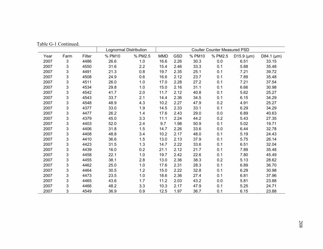
208
Table G-1 Continued. Lognormal Distribution Coulter Counter Measured PSD
Year Farm Filter % PM10 % PM2.5 MMD GSD % PM10 % PM2.5 D15.9 (μm) D84.1 (μm) 2007 3 4486 26.6 1.0 16.6 2.26 30.3 0.0 6.51 33.15 2007 3 4550 31.6 2.2 15.4 2.46 33.3 0.1 5.88 35.48 2007 3 4491 21.3 0.8 19.7 2.35 25.1 0.1 7.21 39.72 2007 3 4508 24.9 0.6 16.6 2.12 23.7 0.1 7.89 35.48 2007 3 4511 26.0 1.0 17.0 2.28 27.2 0.1 7.21 37.54 2007 3 4534 29.8 1.0 15.0 2.16 31.1 0.1 6.66 30.98 2007 3 4542 41.7 2.0 11.7 2.12 40.8 0.1 5.62 25.27 2007 3 4543 33.7 2.1 14.4 2.36 34.5 0.1 6.15 34.29 2007 3 4548 48.9 4.3 10.2 2.27 47.9 0.2 4.91 25.27 2007 3 4377 33.0 1.9 14.5 2.33 33.1 0.1 6.29 34.29 2007 3 4477 26.2 1.4 17.6 2.43 29.0 0.0 6.89 40.63 2007 3 4379 45.0 3.3 11.1 2.24 44.2 0.2 5.43 27.35 2007 3 4403 52.0 2.4 9.7 1.98 50.9 0.1 5.02 19.71 2007 3 4406 31.8 1.5 14.7 2.26 33.6 0.0 6.44 32.78 2007 3 4408 48.8 3.4 10.2 2.17 48.0 0.1 5.19 24.43 2007 3 4410 36.6 1.5 13.0 2.13 37.9 0.1 5.75 26.14 2007 3 4423 31.5 1.3 14.7 2.22 33.6 0.1 6.51 32.04 2007 3 4439 16.0 0.2 21.1 2.12 21.7 0.1 7.89 35.48 2007 3 4458 22.1 1.0 19.7 2.42 22.6 0.1 7.80 45.49 2007 3 4455 38.1 2.8 13.0 2.36 38.3 0.2 5.13 28.62 2007 3 4462 25.0 1.0 17.6 2.31 28.3 0.1 6.89 36.70 2007 3 4464 30.5 1.2 15.0 2.22 32.8 0.1 6.29 30.98 2007 3 4473 23.5 1.0 18.6 2.36 27.4 0.1 6.81 37.96 2007 3 4465 43.6 1.7 11.2 2.03 43.2 0.0 5.81 23.88 2007 3 4466 48.2 3.3 10.3 2.17 47.9 0.1 5.25 24.71 2007 3 4549 36.9 0.9 12.5 1.97 36.7 0.1 6.15 23.88

209
Table G-2. Summary statistics for the particle size distribution analyses on the source sampler filters from 2007. All particle diameters are reported in terms of aerodynamic equivalent diameter.
Lognormal Distribution Coulter Counter Measured PSD Filter % PM10 % PM2.5 MMD GSD % PM10 % PM2.5 D15.9 (μm) D84.1 (μm) Net Mass (g)
83 90.3 2.2 5.8 1.52 89.22 0.27 3.83 8.83 0.22840 84 89.8 2.0 5.9 1.52 88.80 0.26 3.87 8.93 0.21122 85 81.2 2.9 6.4 1.64 79.69 0.17 4.14 11.20 0.57438 86 90.1 1.9 5.9 1.51 88.69 0.22 3.91 8.93 0.39247 87 89.7 2.5 5.8 1.54 87.57 0.21 3.87 9.14 0.37784 88 91.0 3.0 5.6 1.54 88.45 0.24 3.78 8.93 0.37685 89 91.9 2.5 5.6 1.51 89.39 0.24 3.83 8.73 0.23713 90 90.0 2.3 5.8 1.53 87.30 0.21 3.91 9.14 0.21466 91 79.2 2.1 6.7 1.63 77.04 0.13 4.33 11.45 0.31577 92 80.7 1.8 6.7 1.60 78.11 0.12 4.33 11.07 0.41133 93 91.9 2.5 5.6 1.51 89.33 0.25 3.78 8.63 0.18200 94 94.4 2.2 5.4 1.47 92.18 0.25 3.74 8.07 0.20352 95 88.0 4.4 5.7 1.62 83.81 0.24 3.78 9.89 0.17838 96 92.6 3.8 5.4 1.54 88.92 0.28 3.66 8.63 0.16188 97 90.4 3.3 5.6 1.55 88.13 0.31 3.70 8.93 0.21026 98 86.9 3.1 5.9 1.59 84.36 0.22 3.87 9.78 0.21795 99 91.6 2.6 5.6 1.52 89.36 0.24 3.78 8.73 0.12973 100 92.6 2.5 5.6 1.50 89.78 0.24 3.78 8.54 0.13718 101 86.3 3.9 5.9 1.63 82.93 0.22 3.87 10.23 0.16551 102 87.9 3.4 5.8 1.59 84.40 0.22 3.87 9.78 0.15757 103 91.6 2.6 5.6 1.52 89.29 0.24 3.78 8.73 0.47415 104 89.5 2.9 5.7 1.55 85.95 0.22 3.87 9.35 0.51428 105 88.2 2.1 6.0 1.54 85.83 0.17 4.00 9.45 0.20530 106 87.6 2.3 6.0 1.55 85.53 0.20 3.96 9.56 0.20768 107 88.0 1.8 6.1 1.53 85.83 0.17 4.05 9.45 0.54115 108 89.2 1.3 6.1 1.49 86.93 0.17 4.14 9.24 0.51261 109 88.6 1.6 6.1 1.51 86.69 0.18 4.09 9.35 0.53870
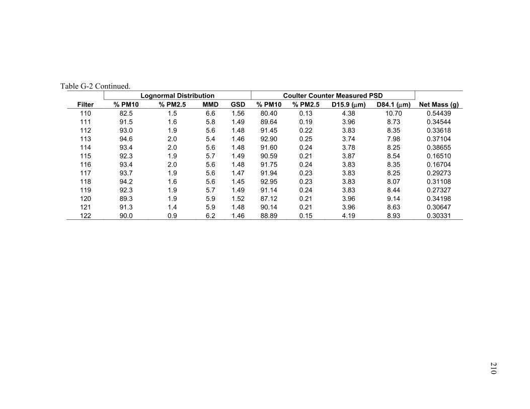
210
Table G-2 Continued. Lognormal Distribution Coulter Counter Measured PSD
Filter % PM10 % PM2.5 MMD GSD % PM10 % PM2.5 D15.9 (μm) D84.1 (μm) Net Mass (g) 110 82.5 1.5 6.6 1.56 80.40 0.13 4.38 10.70 0.54439 111 91.5 1.6 5.8 1.49 89.64 0.19 3.96 8.73 0.34544 112 93.0 1.9 5.6 1.48 91.45 0.22 3.83 8.35 0.33618 113 94.6 2.0 5.4 1.46 92.90 0.25 3.74 7.98 0.37104 114 93.4 2.0 5.6 1.48 91.60 0.24 3.78 8.25 0.38655 115 92.3 1.9 5.7 1.49 90.59 0.21 3.87 8.54 0.16510 116 93.4 2.0 5.6 1.48 91.75 0.24 3.83 8.35 0.16704 117 93.7 1.9 5.6 1.47 91.94 0.23 3.83 8.25 0.29273 118 94.2 1.6 5.6 1.45 92.95 0.23 3.83 8.07 0.31108 119 92.3 1.9 5.7 1.49 91.14 0.24 3.83 8.44 0.27327 120 89.3 1.9 5.9 1.52 87.12 0.21 3.96 9.14 0.34198 121 91.3 1.4 5.9 1.48 90.14 0.21 3.96 8.63 0.30647 122 90.0 0.9 6.2 1.46 88.89 0.15 4.19 8.93 0.30331

211
Table G-3. Summary statistics for the particle size distribution analyses on the PM <100 μm captured in the source sampler cyclone bucket. All particle diameters are reported in terms of aerodynamic equivalent diameter.
Lognormal Distribution Coulter Counter Measured PSD Filter % PM10 % PM2.5 MMD GSD % PM10 % PM2.5 D15.9 (μm) D84.1 (μm) Net Mass (g)
SSAW01 26.82 0.45 15.4 2.00 27.63 0.04 7.54 30.28 8.50696 SSAW02 26.59 0.55 15.7 2.06 27.79 0.04 7.37 31.33 7.32133 SSAW03 24.03 0.68 17.4 2.19 24.78 0.04 7.71 37.12 4.89988 SSAW04 24.60 0.52 16.6 2.10 25.59 0.04 7.63 33.53 8.26629 SSAW05 24.03 0.33 16.3 1.99 25.51 0.04 7.80 30.98 11.30808 SSAW06 25.42 0.31 15.5 1.95 26.54 0.03 7.54 28.62 8.75216 SSAW07 21.08 0.24 17.4 1.99 22.37 0.03 8.16 32.41 9.76915 SSAW08 19.36 0.16 17.8 1.95 21.77 0.03 8.35 31.68 5.35671 SSAW09 29.31 0.61 14.7 2.03 29.77 0.04 7.05 28.94 6.43266 SSAW10 19.62 0.32 18.8 2.10 21.43 0.05 8.25 36.29 4.15692

212
VITA
John David Wanjura 201 Scoates Hall MS 2117 - TAMU c/o Department of Biological and Agricultural Engineering Texas A&M University College Station, TX 77843-2117 EDUCATION Doctor of Philosophy in Biological and Agricultural Engineering; Texas A&M University (May 2008) Master of Science in Biological and Agricultural Engineering; Texas A&M University (May 2005) Bachelor of Science in Agricultural Engineering; Texas A&M University (May 2005) Bachelor of Science in Agricultural Systems Management; Texas A&M University (May 2002) HONORS Alpha Epsilon Honor Fraternity Eagle Scout Phi Eta Sigma Gamma Sigma Delta Honor Society PREVIOUSLY PUBLISHED MATERIAL Wanjura, J.D., C.B. Parnell, Jr., B.W. Shaw, and R.E. Lacey. 2005. Design and
evaluation of a low volume total suspended particulate sampler. Trans. ASAE 48(4): 1547-1552.
Wanjura, J.D., M.D. Buser, C.B. Parnell, B.W. Shaw, and R.E. Lacey. 2005. A simulated approach to estimating PM10 and PM2.5 concentrations downwind from cotton gins. Trans. ASAE 48(5): 1919-1925.
Wanjura, J.D., C.B. Parnell, B.W. Shaw, S.C. Capareda. 2006. Particle size distribution of PM emitted from cotton harvesting. ASABE Paper No. 064168. St. Joseph, MI.: ASABE.
Wanjura, J.D., B.W. Shaw, C.B. Parnell, Jr., R.E. Lacey, and S.C. Capareda. 2007. Comparison of continuous monitor (TEOM) vs. gravimetric sampler particulate matter concentrations. Submitted for publication in Trans. ASAE, 2007.