a seamless, high-resolution, coastal digital elevation model (dem

A Seamless, High-Resolution, Coastal Digital Elevation Model (DEM) for Southern California

U.S. Department of the InteriorU.S. Geological Survey

Data Series 487

COVEROblique 3-D image of La Jolla Submarine Canyon and the La Jolla coastline in central San Diego County, California.


By Patrick L. Barnard and Daniel Hoover

Data Series 487

U.S. Department of the InteriorU.S. Geological Survey

U.S. Department of the InteriorKEN SALAZAR, Secretary

U.S. Geological SurveyMarcia K. McNutt, Director

U.S. Geological Survey, Reston, Virginia: 2010

For product and ordering information:World Wide Web: http://www.usgs.gov/pubprodTelephone: 1-888-ASK-USGS

For more information on the USGS—the Federal source for science about the Earth,its natural and living resources, natural hazards, and the environment:World Wide Web: http://www.usgs.govTelephone: 1-888-ASK-USGS

Any use of trade, product, or firm names is for descriptive purposes only and does not imply endorsement by the U.S. Government.

Although this report is in the public domain, permission must be secured from the individual copyright owners to reproduce any copyrighted material contained within this report.

Suggested citation:Barnard, P.L., and Hoover, D., 2010, A seamless, high-resolution coastal digital elevation model (DEM) for southern California. U.S. Geological Survey Data Series 487, 8 p.

http://www.usgs.gov/pubprod

http://www.usgs.gov

iii

Contents

Introduction.....................................................................................................................................................1DEM Construction Methods .........................................................................................................................1DEM Construction Overview ........................................................................................................................2

DEM Construction Procedures ...........................................................................................................3DEM Accuracy and Limitations ..........................................................................................................4

The Digital Files ..............................................................................................................................................7Acknowledgments .........................................................................................................................................8Reference Cited..............................................................................................................................................8

Figures

Figure 1. Southern California location map and identifiers (IDs) for the 45 individual Digital Elevation Models (DEMs). ...............................................................................................................1

Figure 2. Areal extent of data sources used for DEM SB4 ....................................................................3Figure 3. Preliminary DEM for SB4 prior to interpolation of data gaps. ...............................................5Figure 4. West end of SB4 showing preliminary DEM and points extracted for use in

interpolating elevations in data gaps. ...........................................................................................5Figure 5. Final DEM for SB4 and onshore to offshore elevation profile along section A-B .............6

Tables

Table 1. Individual DEM names and locations, listed from south to north ..........................................2Table 2. Geospatial statistics of the DEMs ...............................................................................................7Table 3. List of DEMs (zipped Arc ASCII grids) by county ......................................................................7

IntroductionA seamless, 3-meter digital elevation model (DEM) was

constructed for the entire Southern California coastal zone, extending 473 km from Point Conception to the Mexican border. The goal was to integrate the most recent, high-resolution datasets available (for example, Light Detection and Ranging (Lidar) topography, multibeam and single beam sonar bathymetry, and Interferometric Synthetic Aperture Radar (IfSAR) topography) into a continuous surface from at least the 20-m isobath to the 20-m elevation contour.

This dataset was produced to provide critical boundary conditions (bathymetry and topography) for a modeling effort designed to predict the impacts of severe winter storms on the Southern California coast (Barnard and others, 2009). The hazards model, run in real-time or with prescribed scenarios,


By Patrick L. Barnard and Daniel Hoover

incorporates atmospheric information (wind and pressure fields) with a suite of state-of-the-art physical process models (tide, surge, and wave) to enable detailed prediction of water levels, run-up, wave heights, and currents. Research-grade predictions of coastal flooding, inundation, erosion, and cliff failure are also included. The DEM was constructed to define the general shape of nearshore, beach and cliff surfaces as accurately as possible, with less emphasis on the detailed variations in elevation inland of the coast and on bathymetry inside harbors. As a result this DEM should not be used for navigation purposes.

DEM Construction MethodsForty-five individual DEMs were constructed (fig. 1; table 1)

using more than 40 bathymetric and topographic data sets. The data sets used are detailed in a downloadable spreadsheet at the

Figure 1. Southern California location map and identifiers (IDs) for the 45 individual Digital Elevation Models (DEMs).

LA1

SD2SD3

SD1

SD5

LA2OC7

OC5OC6

VE2

SD9

VE4

SD6

VE3

LA7

SD8SD7

SB1VE5

SD4

SD11

SB4SB3

OC1OC2

LA11 LA8

SD10

VE6SB5SB9

LA5

SB8

VE1

LA6

LA4

LA9

OC3

SB6

OC4

SB10

LA3

120°W

34°N

33°N

119°W 118°W 117°W

Index Map0 10050

Kilometers

2 A Seamless, High-Resolution, Coastal Digital Elevation Model (DEM) for Southern California

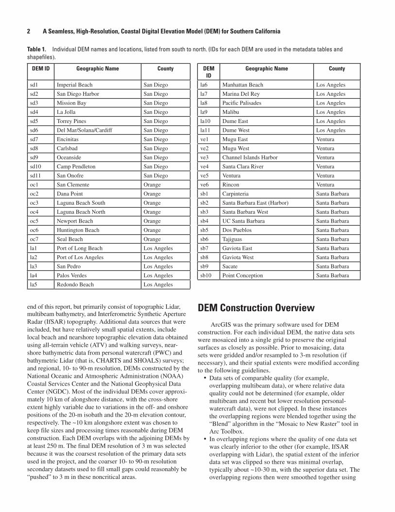
end of this report, but primarily consist of topographic Lidar, multibeam bathymetry, and Interferometric Synthetic Aperture Radar (IfSAR) topography. Additional data sources that were included, but have relatively small spatial extents, include local beach and nearshore topographic elevation data obtained using all-terrain vehicle (ATV) and walking surveys, near-shore bathymetric data from personal watercraft (PWC) and bathymetric Lidar (that is, CHARTS and SHOALS) surveys; and regional, 10- to 90-m resolution, DEMs constructed by the National Oceanic and Atmospheric Administration (NOAA) Coastal Services Center and the National Geophysical Data Center (NGDC). Most of the individual DEMs cover approxi-mately 10 km of alongshore distance, with the cross-shore extent highly variable due to variations in the off- and onshore positions of the 20-m isobath and the 20-m elevation contour, respectively. The ~10 km alongshore extent was chosen to keep file sizes and processing times reasonable during DEM construction. Each DEM overlaps with the adjoining DEMs by at least 250 m. The final DEM resolution of 3 m was selected because it was the coarsest resolution of the primary data sets used in the project, and the coarser 10- to 90-m resolution secondary datasets used to fill small gaps could reasonably be “pushed” to 3 m in these noncritical areas.

DEM Construction OverviewArcGIS was the primary software used for DEM

construction. For each individual DEM, the native data sets were mosaiced into a single grid to preserve the original surfaces as closely as possible. Prior to mosaicing, data sets were gridded and/or resampled to 3-m resolution (if necessary), and their spatial extents were modified according to the following guidelines.•Data sets of comparable quality (for example,

overlapping multibeam data), or where relative data quality could not be determined (for example, older multibeam and recent but lower resolution personal-watercraft data), were not clipped. In these instances the overlapping regions were blended together using the “Blend” algorithm in the “Mosaic to New Raster” tool in Arc Toolbox.

• In overlapping regions where the quality of one data set was clearly inferior to the other (for example, IfSAR overlapping with Lidar), the spatial extent of the inferior data set was clipped so there was minimal overlap, typically about ~10-30 m, with the superior data set. The overlapping regions then were smoothed together using

DEM ID Geographic Name County DEM ID

Geographic Name County

sd1 Imperial Beach San Diego la6 Manhattan Beach Los Angeles

sd2 San Diego Harbor San Diego la7 Marina Del Rey Los Angeles

sd3 Mission Bay San Diego la8 Pacific Palisades Los Angeles

sd4 La Jolla San Diego la9 Malibu Los Angeles

sd5 Torrey Pines San Diego la10 Dume East Los Angeles

sd6 Del Mar/Solana/Cardiff San Diego la11 Dume West Los Angeles

sd7 Encinitas San Diego ve1 Mugu East Ventura

sd8 Carlsbad San Diego ve2 Mugu West Ventura

sd9 Oceanside San Diego ve3 Channel Islands Harbor Ventura

sd10 Camp Pendleton San Diego ve4 Santa Clara River Ventura

sd11 San Onofre San Diego ve5 Ventura Ventura

oc1 San Clemente Orange ve6 Rincon Ventura

oc2 Dana Point Orange sb1 Carpinteria Santa Barbara

oc3 Laguna Beach South Orange sb2 Santa Barbara East (Harbor) Santa Barbara

oc4 Laguna Beach North Orange sb3 Santa Barbara West Santa Barbara

oc5 Newport Beach Orange sb4 UC Santa Barbara Santa Barbara

oc6 Huntington Beach Orange sb5 Dos Pueblos Santa Barbara

oc7 Seal Beach Orange sb6 Tajiguas Santa Barbara

la1 Port of Long Beach Los Angeles sb7 Gaviota East Santa Barbara

la2 Port of Los Angeles Los Angeles sb8 Gaviota West Santa Barbara

la3 San Pedro Los Angeles sb9 Sacate Santa Barbara

la4 Palos Verdes Los Angeles sb10 Point Conception Santa Barbara

la5 Redondo Beach Los Angeles

Table 1. Individual DEM names and locations, listed from south to north. (IDs for each DEM are used in the metadata tables and shapefiles).

DEM Construction Overview 3

SB5

SB4SB3

Data Coverage Areas

University of Texas Lidar (2005)

CSUMB Multibeam Bathymetry (2007)

USGS Multibeam Bathymetry (2007)

USGS Multibeam Bathymetry (2006)

USGS Single Beam Bathymetry (2006)

NOAA IfSAR (2002-2003)

NOAA Tsunami DEM

0 52.5

Kilometers

Data gap

Data gap

N

the Blend algorithm. This range of overlap was found to be the most efficient for ensuring a smooth transition between data sets while minimizing the use of lower quality data.

DEM Construction Procedures

1. Divide study area into ~10 km alongshore segments •Define DEM coverage area/polygon that extends ~10

km alongshore from -20 m isobath to 20-m topographic contour, or to 750 m from back beach, whichever is longer

•Ensure that adjacent DEM coverage areas overlap by ~ 250 m

•Cut off DEMs at county boundaries with ~500 m overlap

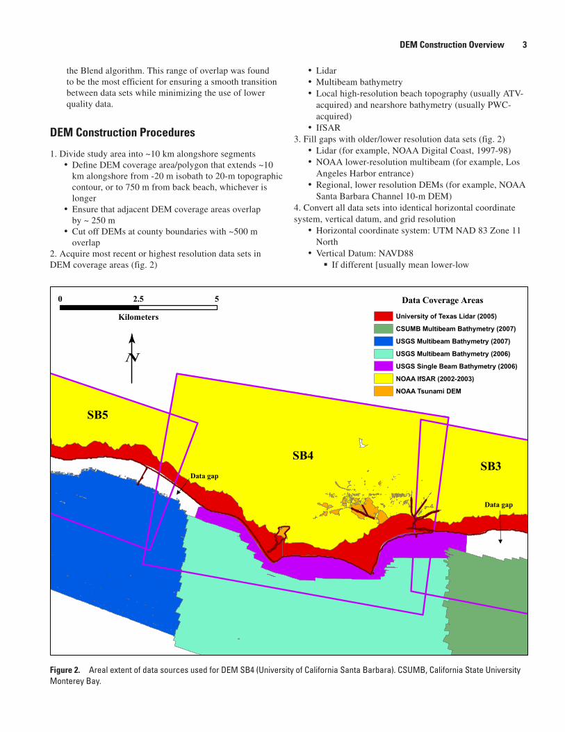
2. Acquire most recent or highest resolution data sets in DEM coverage areas (fig. 2)

•Lidar•Multibeam bathymetry•Local high-resolution beach topography (usually ATV-

acquired) and nearshore bathymetry (usually PWC-acquired)

• IfSAR3. Fill gaps with older/lower resolution data sets (fig. 2)

•Lidar (for example, NOAA Digital Coast, 1997-98)•NOAA lower-resolution multibeam (for example, Los

Angeles Harbor entrance)•Regional, lower resolution DEMs (for example, NOAA

Santa Barbara Channel 10-m DEM)4. Convert all data sets into identical horizontal coordinate system, vertical datum, and grid resolution

•Horizontal coordinate system: UTM NAD 83 Zone 11 North

•Vertical Datum: NAVD88If different [usually mean lower-low

Figure 2. Areal extent of data sources used for DEM SB4 (University of California Santa Barbara). CSUMB, California State University Monterey Bay.


water(MLLW)], convert using local NOAA tide station information [http://tidesandcurrents.noaa.gov/ (last accessed December 2, 2009)] based on survey metadata

•Grid resolution: 3 mIf already gridded at higher (<3-m), or lower

resolution (up to 10-m resolution), resample to 3 m using bilinear interpolation

If already gridded at resolution of ≥10-m, export as xyz, reimport as xyz, create TIN (triangular irregular network), create 3-m grid from TIN using linear interpolation of the TIN triangles, and clip to survey extent

Ungridded:•Lidar (topography), 3-m grid using natural-

neighbor interpolation to preserve abrupt elevation changes (for example, beaches backed by cliffs)

•Multibeam, 3-m grid using inverse distance weighting using “Average Gridder” in Fledermaus (ideal for data sets having more than 10 million points)

•Lower resolution surveys (for example, PWC-collected bathymetry): create TIN from points then convert to 3-m grid using linear interpolation of the TIN triangles

5. Clip data sets to DEM/coverage needs, if necessary•Useful for data management and processing efficiency •Necessary for very large data sets, such as county-wide

IfSAR, or very large Lidar data sets (for example, Los Angeles County)

• Clip ocean and waves from topographic Lidar and IfSARClip water level by determining sea level at time of

survey then using “Extract by Attributes” tool in Arc Toolbox

Clip wave crests manually using mask

6. Manage overlapping data sets• Data sets allowed to overlap extensively only if they are

of comparable quality, otherwise allow only minimal (~10–30 m) overlap to ensure smooth DEM transitions

•Clip IfSAR data (lower quality) to minimal overlap with topographic Lidar (better quality)

•Clip low-resolution data sets “pushed” to 3-m resolution, such as Personal Watercraft data and regional DEMs, to minimal overlap with adjacent high-resolution data sets (usually multibeam and topographic Lidar)

•Extensive overlap between adjacent Lidar and multibeam data sets is rare but allowed as quality is comparable

7. Fill in data gaps between high-resolution data sets• If no high-resolution data are available between the

10-m isobath and coastal Lidar, in protected harbors/embayments, or in other areas where interpolation from surrounding data sets will create a surface unlikely to

reflect actual bathymetry/topography accurately, fill in gaps with regional DEMs or other low-resolution data sets. Otherwise, interpolate across gaps.Filling in using regional DEMs/other low-

resolution data:•Clip best available regional DEM to gap area,

allowing only minimal overlap (~10-30 m) with adjacent high-resolution data sets

•Export clipped grid as xyz, reimport as points, create TIN, create 3-m grid from TIN, clip to gap extent

Interpolation:•Create preliminary DEM using Mosaic tool

(fig. 3) with the following settings:•Coordinate System: UTM Zone 11 North

Pixel Type: 32_Bit_FloatCell Size: 3 Mosaic Method: BlendMosaic Color Map: Last

•Create mask of data gap(s) to fill with preliminary DEM surface, ensuring minimal overlap with surrounding data

•Clip preliminary DEM with mask, export clipped grid as xyz, reimport as points (fig. 4), create TIN, create 3-m grid from TIN, clip to gap extent

8. Compile final DEMs•Load all data sets for DEM•Verify all significant data gaps filled (few missing cells

OK) in DEM coverage area•Build DEM using “Mosaic to New Raster” tool in

ArcGIS with same setting as noted above in Step 7•Clip DEM to DEM coverage area (fig. 5)•Create contours and plot cross-shore profiles to verify

data quality and consistency

DEM Accuracy and LimitationsOriginal data were preserved as much as possible

by minimizing exporting, regridding, smoothing and/or resampling during the DEM construction process. However, the vertical accuracy of the resulting DEM is only as good as the accuracy of the native data, which varies considerably. Vertical accuracy reported by the data-source agencies ranges from about ±8 cm for most of the Lidar data to about ±1 m for IfSAR data. The final DEMs have been reviewed and corrections have been applied for obvious anomalies, but we have not thoroughly analyzed the native data sets to determine whether the reported horizontal and vertical uncertainties are correct. We also assume that grids provided to us were constructed using appropriate techniques and in the proper resolution from cleaned point data, which often were not available to us. Users should contact the original data sources for inquiries about all metadata and related issues, such as data

http://tidesandcurrents.noaa.gov/

http://tidesandcurrents.noaa.gov/

DEM Accuracy and Limitations 5

SB4SB3

SB5

5 m contours

High: 179

Low: -87

0 52.5

Kilometers

Data gap

SB4 elevation (m)

N

Figure 3. Preliminary DEM for SB4 prior to interpolation of data gaps and clipping to DEM area.

Figure 4. West end of SB4 showing preliminary DEM and points extracted for use in interpolating elevations in data gaps.

N

SB5

SB4SB4

Extracted pointsfor extrapolation

5 m contours

High: 179

Low: -87

SB4 elevation (m)

0 250

Kilometers

500


Figure 5. Final DEM for SB4 (top) and onshore to offshore elevation profile along section A-B (bottom).

SB4

SB3

SB5

0 52.5

Kilometers

B

A

5 m contours

High: 179

Low: -52

SB4 elevation (m)

N

accuracy or consistency. No guarantee is given for the quality of any of the data. Users must carefully consider the inherent limitations and potential issues associated with these data when using these grids.

The coastal zone is an extremely dynamic environment. Single storms can modify local beach and nearshore elevations by more than one meter and move elevation contours horizon-

tally by tens of meters; and seasonal and interannual changes can significantly affect coastal bathymetry and topography. Because the data sets used for the DEM were obtained at different times (mostly from 2005 to 2008) and at different resolutions, we make no assurances regarding the local accuracy of the DEM surface. However, where possible, we used data collected in the fall to minimize the potential for winter storm effects.

0 1,000 2,000 3,000 4,000 5,000 6,000−50

0

50

100

150

Profile A–B

Distance (m)

Ele

vati

on (

m)

The Digital Files 7

DEM ID SurfaceArea (km2)

MinimumElevation (m)

MaximumElevation (m)

MeanElevation (m)

sd2 238.8 -52.8 156.0 13.7

sd3 178.2 -43.6 154.6 35.3

sd4 64.2 -149.5 258.2 44.2

sd5 133.3 -486.1 155.8 -8.4

sd6 129.0 -37.6 138.0 45.0

sd7 80.9 -40.2 140.2 40.7

sd8 84.5 -84.0 127.3 20.5

sd9 151.7 -30.4 221.1 28.5

sd10 57.9 -30.0 225.4 2.1

sd11 75.4 -31.4 374.9 32.5

oc1 65.1 -46.0 271.5 21.0

oc2 63.0 -48.8 268.6 44.4

oc3 41.1 -66.5 287.2 62.5

oc4 34.3 -76.2 233.4 40.8

oc5 206.2 -221.6 89.6 7.1

oc6 184.7 -23.9 48.9 4.1

oc7 206.2 -39.0 48.0 5.0

la1 320.8 -28.3 109.2 11.4

la2 322.3 -34.8 138.9 14.6

la3 22.4 -39.5 287.6 42.0

la4 38.9 -393.6 398.8 102.7

la5 45.4 -292.6 345.9 -3.0

la6 39.3 -90.4 68.0 -4.5

la7 126.9 -28.5 145.7 21.1

la8 51.9 -26.6 536.1 45.0

la9 38.7 -34.5 485.4 72.1

la10 41.1 -51.1 311.5 11.9

la11 64.6 -194.5 357.7 11.0

ve1 39.6 -118.4 386.3 36.4

ve2 169.7 -303.9 475.9 17.0

ve3 134.3 -251.2 57.5 -0.3

ve4 153.0 -24.5 282.3 6.7

ve5 78.7 -26.5 380.0 39.8

ve6 47.5 -23.0 321.0 37.7

sb1 72.5 -33.0 222.0 13.1

sb2 47.2 -39.3 152.1 8.9

sb3 55.7 -44.4 191.2 23.5

sb4 55.9 -51.9 178.8 16.9

sb5 42.0 -59.4 179.1 11.8

sb6 29.9 -42.4 260.5 52.6

sb7 27.4 -51.8 235.3 14.9

sb8 38.0 -61.0 306.6 24.2

sb9 41.9 -51.1 198.6 1.1

sb10 37.4 -74.8 185.9 19.5

Mean (All-DEMs)

96.1 -89.0 234.4 24.4

Table 2. Geospatial statistics of the DEM’s.

Table 3. List of DEMs (zipped Arc ASCII grids) by county.

DEM bathymetry in harbors should be used with extreme caution. Only rarely was high-resolution multibeam data available in harbors, and as these areas were not crucial for our project objectives we often used low-resolution, 10- to 90-m DEMs. These DEMs presumably were constructed from various NOAA National Ocean Service (NOS) survey datasets, but native datasets for these DEMs were not reviewed for this project. Therefore, harbors may have the least accurate bathymetries in the DEM. Piers commonly were included in Lidar data, and although piers usually act as semi permeable barriers to waves, tidal currents, and littoral transport, they appear as impermeable barriers in the DEM.

Table 2 lists some basic geospatial statistics of the final DEMs. Preliminary analysis of the overlapping DEM regions in Santa Barbara County indicates that individual grid cell elevation offsets along the coastal strip (approximately ±500 m cross-shore) are almost always < 10 cm, and mean elevation offsets for the entire overlapping region between all DEMs is ~2 cm. Most of the bias can be attributed to grid-cell misalignments (that is, areas where grid cells in adjacent DEMs are not aligned) in the upper elevations of the DEMS where steep slopes are common, far removed from the active coastal zone. This analysis suggests a high level of internal precision in DEM production, but the accuracy of the native data sets relative to user needs still must be carefully considered when using these DEMs.

The Digital Files

For all spatial data files the horizontal coordinate system is Universal Transverse Mercator (UTM), Zone 11 North, North American Datum of 1983 (NAD83). All eleva-tions are relative to the North American Vertical Datum of 1988 (NAVD88).

Each of the 45 DEMs is posted as a 3-m resolution Arc ASCII grid (table 3). Arc ASCII grids can easily be converted to ARC raster grids using Arc Toolbox. A variety

San Diego

Orange County

Los Angeles

VenturaSanta

Barbara

sd1.zipsd2.zipsd3.zipsd4.zipsd5.zipsd6.zipsd7.zipsd8.zipsd9.zip

sd10.zipsd11.zip

oc1.zipoc2.zipoc3.zipoc4.zipoc5.zipoc6.zipoc7.zip

la1.zipla2.zipla3.zipla4.zipla5.zipla6.zipla7.zipla8.zipla9.zip

la10.zipla11.zip

ve1.zipve2.zipve3.zipve4.zipve5.zipve6.zip

sb1.zipsb2.zipsb3.zipsb4.zipsb5.zipsb6.zipsb7.zipsb8.zipsb9.zip


of other GIS-related software packages also can handle this format, including Surfer, Global Mapper, Fledermaus, and Imagine.

There are two polygon shapefiles; DEMCoverageAreas.zip and DataCoverageAreas.zip (with layer file). The first shapefile shows the DEM coverage areas for all 45 DEMs (fig. 1). The second shapefile shows the coverage area for each of the native data sets, with fields displaying key metadata, such as the data source and resolution.

Finally, there is a Microsoft Excel spreadsheet (DEM_Metadata.xls) that lists all primary metadata for all the data sets used in this project, as well as the dataset components for each of the 45 individual DEMs, grouped by county.

Polygon ShapefilesDEMCoverageAreas.zipDataCoverageAreas.zip (with layer file)

SpreadsheetDEM_Metadata.xls

AcknowledgmentsMany thanks to Pete Dartnell, Pat Iampietro, Randy

Bucciarelli, and David Finlayson for providing newly released data to support this project. This project was funded by the USGS Coastal and Marine Geology Program and the USGS Multihazards Demonstration Project in Southern Cali-fornia. Florence Wong and Theresa Fregoso provided helpful internal reviews.

Reference CitedBarnard, P.L., O’Reilly, B., van Ormondt, M., Elias, E.,

Ruggiero, P., Erikson, L.H., Hapke, C., Collins, B.D., Guza, R.T., Adams, P.N. and Thomas, J.T., 2009, The framework of a coastal hazards model—A tool for predicting the impact of severe storms: U.S. Geological Survey Open-File Report 2009-1073, 21 p., http://pubs.usgs.gov/of/2009/1073/ (last accessed December 2, 2009).

http://pubs.usgs.gov/of/2009/1073/

Produced in the Western Region, Menlo Park, CaliforniaManuscript approved for publication, November 27, 2009Text edited by Tracey SuzukiLayout and Design by Jeanne S. DiLeo

Barnard and H

oover—A Seam

less, High-Resolution, Coastal Digital Elevation Model (DEM

) for Southern California—D

ata Series 487

a seamless, high-resolution, coastal digital elevation model (dem

Documents