"a 'second opinion' on the economic health of the american ... · a “second...

National Tax Journal, March 2012, 65 (1), 7–32

A “SECOND OPINION” ON THE ECONOMIC HEALTH OF THE AMERICAN MIDDLE CLASS

Richard V. Burkhauser, Jeff Larrimore, and Kosali I. Simon

Researchers considering levels and trends in the resources available to the middle class traditionally measure the pre-tax cash income of tax units or the pre-tax, post-transfer, size-adjusted income of households. Choices regarding the income measure and sharing unit to be analyzed, as well as other methodological choices, carry signifi cant implications for assessing income trends. In particular, we show that focusing on tax units rather than households and not adjusting for sharing unit size greatly reduces measured growth in middle class income, as does excluding the effect of taxes and the value of in-kind benefi ts. As an example, we demonstrate how much these distinctions change the observed distribution of benefi ts from the tax exclusion of employer provided health insurance.

Keywords: middle class, health insurance tax exclusion, median income, sharing unit, income distribution

JEL Codes: D31, H20, I18

I. INTRODUCTION

The most basic measure of the economic resources available to the average American — median household income — has been consistently tracked by the U.S. Census

Bureau since 1967 using yearly data from the March Current Population Survey (CPS). While median income has fallen during economic downturns and risen with recovery within all business cycles, yearly gains have historically more than offset yearly losses so that median income has risen from peak-to-peak over each business cycle. That is, the real, infl ation-adjusted income of middle class households as measured by median household income has consistently grown over time, controlling for short-term market

Richard V. Burkhauser: Department of Policy Analysis and Management, Cornell University, Ithaca, NY, USA ([email protected])Jeff Larrimore: Joint Committee on Taxation, U.S. Congress, Washington, DC, USA (jeff [email protected])Kosali I. Simon: School of Public and Environmental Aff airs, Indiana University, Bloomington, IN, USA ([email protected])

National Tax Journal8

1 An alternative way to measure how middle class Americans have fared over time is to use panel data that actually follows the same individuals over time. Such longitudinal analyses are not possible with the March CPS data. For an example of this type of analysis, see Auten and Gee (2009).

conditions. However, this was not the case over the peak years (2000–2007) of the fi rst business cycle of the 21st century when median household income fell by 0.1 percent (DeNavas-Walt, Proctor, and Smith, 2008).

This highly visible measure of the decline in the real economic resources available to middle class Americans is often discussed alongside research using Internal Rev-enue Service (IRS) administrative records by Piketty and Saez (2003) and Saez (2009) showing that the fraction of market income going to the top 10 percent of tax units is at its highest level since at least 1917. Together, these fi ndings suggest that the middle class is not sharing proportionately in the fruits of American economic growth. Such concerns have been manifested in the popular new media (Johnson, 2007; Piketty and Saez, 2007; Goldman, 2008; Lahart and Evans, 2008; Leonhardt, 2008), and have led to calls for policies that would increase the share of income growth going to the middle of the income distribution. For instance, when forming the White House Task Force on Middle Class Working Families in 2009, President Barack Obama said, “Middle class Americans have been working harder, yet not enjoying their fair share of the fruits of a growing economy” (Obama, 2009).

In this paper, we offer new evidence that forms a “second opinion” on the extent to which middle class Americans have failed to benefi t from economic growth over the past three business cycles (1979–2007). Using cross-sectional data to capture the eco-nomic resources available to individuals at the same point in the income distribution over time, we fi nd that the evidence of a middle class decline is far from clear, and that such results are highly sensitive to how available resources are measured.1 Thus, we will argue that the apparent failure of the median American to benefi t from economic growth can largely be explained by the use of an income measure for this purpose that does not fully capture what is actually happening to the resources available to middle class individuals.

Researchers considering long term income trends have traditionally based their analyses on one of two data sources. The fi rst, used by Piketty and Saez (2003) and others, is IRS tax record data. These IRS tax records contain information on the pre-tax, pre-transfer cash income of tax units — the group of individuals who fi le a tax return together and their child dependents. These data, occasionally supplemented with income estimates for non-fi ling tax units, provide an excellent measure of the distribution of cash market income among tax units.

The second data source, reported each year by the Census Bureau (DeNavas-Walt, Proctor, and Smith, 2008), comes from the annual March CPS. These data contain information on the pre-tax, post-transfer cash income of households excluding capital gains. In addition to the taxable income reported on tax records, this CPS-based measure also includes the value of all public transfers (including welfare, Social Security, and other government provided cash assistance) received by the household, much of which

The Economic Health of the American Middle Class 9

is not taxable. Thus, the CPS-based income defi nition is intended to capture resources coming from cash income regularly received by the household, regardless of whether it comes from market-based activities. It excludes, however, some irregularly received income such as capital gains from investments or home sales, non-cash government transfers, and employer provided in-kind compensation. It also excludes resources that affect consumption but are excluded from income both in government income statistics and tax collection, such as the imputed rent of owner-occupied housing.

The distinction between tax units or households as the sharing units to be analyzed or the choice of the resources counted as income are somewhat abstract concepts and may appear to be trivial. As a result, literatures that differ in their income measures of choice or sharing units are often viewed interchangeably. Indeed, it is often the case that an individual’s tax unit and household unit are exactly the same. A tax unit typically consists of an adult, his or her spouse, and any dependent children. Such a tax unit would include all of the members of a “traditional family arrangement” household. However, there are many situations in which this is not the case. For example, cohabiters, roommates who share expenses, children who move back in with their parents, or older parents who live with their adult children are households that contain more than one tax unit.

If measures of the level and trend in the shared resources of middle class individuals were insensitive to the choice of sharing unit, then these differences would be immate-rial. However, we will show that the choice of sharing unit and which of its resources are counted as income makes a substantive difference in measures of the resources available to middle class Americans, as will controlling for the number of people in the sharing unit. Furthermore, the inclusion of taxes and transfers, in addition to the value of employer provided health insurance benefi ts, Medicare, and Medicaid, further impacts the observed trend in resources available to the middle class.

Several earlier papers have recognized the importance of income defi nitions in evaluating economic resources. For example, Karoly (1994) shows how much including different mixes of taxes and income transfers impacts family income inequality. Simi-larly, Meyer and Sullivan (2009b) show how pre-tax and post-tax income defi nitions impact measures of poverty in their argument that consumption based measures would more precisely capture poverty trends. Additionally, both the European Union and the Organisation for Economic Co-operation and Development (OECD) use a post-tax, post-transfer based poverty measure rather than a pre-tax, post-transfer measure because the former more closely mirrors personal consumption (d’Ercole and Förster, forthcoming).

Others have recognized the importance of including the value of in-kind compensa-tion in measures of market income, since cash compensation alone does not provide a complete measure of payment for work. For example, Pierce (2001, 2010) uses the Employment Cost Index (ECI) data to consider how levels and trends in labor compen-sation change when he includes employer contributions to fringe benefi ts (including health insurance). Chung (2003) extends this insight by merging data from the ECI into the CPS. Additionally, previous research by Burkhauser et al. (forthcoming) demonstrates how choices of income defi nition impact measures of income inequality at the top of the income distribution, and Meyer and Sullivan (2009a) consider similar


questions for income inequality measured using 90/10 ratios — the ratio of the income of the individual at the 90th percentile of the income distribution to that of the individual at the 10th percentile.

Here, we expand on this previous research by using March CPS data to report the median resources of Americans as well as the growth in those resources by quintile over the last three business cycles (1979–1989, 1989–2000, and 2000–2007), using different assumptions regarding the sharing unit, tax treatment of income, and the various sources of income we include in our resource measure. When we analyze median income in the CPS data using tax units, we fi nd that the pre-tax, pre-transfer income (the market income) of the median tax unit decreased over the 2000–2007 business cycle. This is the case whether we focus solely on those tax units who fi le a return or on all tax units regardless of whether they fi le a return. Potentially more disturbing, the median pre-tax, pre-transfer income of all tax units (fi lers and non-fi lers) only increased by 3.2 percent in real terms over the entire period between 1979–2007. These results are consistent with the view that the typical American has not gained much from economic growth over the last 30 years.

But when we broaden the sharing unit to the household, account for economies of scale in household consumption, and recognize that the payment of taxes or the receipt of tax credits as well as government transfer income and in-kind benefi ts all impact the economic resources available to individuals, we fi nd the story changes. Specifi cally, when using our broadest measure of available resources — post-tax, post-transfer, size-adjusted household income including the ex-ante value of in-kind health insurance benefi ts — median income growth of individual Americans improves to 36.7 percent over the period from 1979–2007, and by 4.8 percent between 2000–2007. Similarly, these choices impact the observed distribution of income and the extent to which incomes at the top of the distribution are growing faster than those of the middle and lower classes.

We then provide an example of why such a broader measure of available economic resources is of value in considering the distributional impacts of public policy. We do so by showing how the distribution of benefi ts from the tax exclusion of employer provided health insurance differs when it is measured across the not-size-adjusted income of tax units and the size-adjusted household income of individuals — two common approaches to capturing such policy effects. Using our broader measure of household-based income, we show that the value to the middle class of the tax exclusion of employer provided health insurance benefi ts is greater than that observed when focusing on tax unit-based income. We conclude that researchers would be well served by using these broader measures of income and sharing unit when considering the distributional impacts of public policy proposals.

II. DATA

To explore the trend in the available resources of middle class Americans over the past 30 years, we use the public use March CPS data set supplemented with cell-means to


overcome topcoding of high incomes in the March CPS.2 One limitation of the CPS data discussed by Ryscavage (1995) and Jones and Weinberg (2000) that remains even with the use of cell-means to overcome topcoding is a change in survey methods between 1992 and 1993 that limits comparability across these years. Thus, in all series the changes in income between 1992 and 1993 are suppressed and assumed to be zero given the trend-break resulting from survey redesign. The approach used in this analysis to overcome this break in the CPS data is similar to that used by Burkhauser et al. (forthcoming) and Atkinson, Piketty, and Saez (2011). Since incomes are being compared across years, all income is adjusted for infl ation to 2008 dollars using the Consumer Price Index Research Series Using Current Methods (Stewart and Reed, 1999).3

While the March CPS is commonly used for measuring levels and trends in income and its distribution in the United States, it does not directly inquire about tax credits, tax liabilities, or about the value of in-kind compensation such as employer or government provided health insurance. To overcome these limitations, we impute this information for each individual to supplement the income data in the March CPS.

To impute tax credits and liabilities, we enter marital status, state of residence, age, number of dependents, detailed income information, and other factors for each tax unit into National Bureau of Economic Research (NBER) TaxSim 9.0 (Feenberg and Coutts, 1993), which uses these data to estimate federal and state income tax liabilities, including Social Security and Medicare payroll taxes, based on the tax laws in effect in each year.4 Since the March CPS samples households, they are divided into tax units prior to imputing tax liabilities. This division is performed using the procedure described in Burkhauser et al. (forthcoming), which mirrors the Piketty and Saez (2003) defi nition of potential tax units. All single individuals age 20 and over, married couples, and divorced or widowed individuals are considered independent tax units.5 Never-married children under age 20 are considered dependents and are assigned to the tax unit of their parent or guardian.6

2 In this procedure, all individuals with income from an income source above the topcode threshold have their income replaced with the mean source-level income of all individuals who are topcoded on that income source. The incomes from all income sources (both the topcoded sources replaced with cell-mean values and the actual values for all other sources) are then combined to yield total personal income. See Larrimore et al. (2008) for further details on the cell-mean series.

3 A more detailed discussion of this issue as it relates to this paper is contained in a data appendix available upon request from the authors.

4 Since the March CPS data do not have detailed information on mortgage interest, property taxes paid, charitable contributions, or other factors relevant for itemized deductions, this imputation likely understates the value of deductions for individuals not taking the standard deduction.

5 Given that many students are dependents even if they fi le their own tax return, we replicated our analysis assuming that students age 20–24 were part of their parents’ tax unit rather than independent tax units. These results, which are largely unchanged, are contained, along with a more detailed discussion of our methods for calculating them, in a data appendix available upon request from the authors.

6 In the small number of cases where never-married individuals under age 20 live in a household without a parent or guardian, we assign them to the tax unit of the household’s primary family or the oldest adult in the household when there is no primary family. Only households with no adults over age 20 are treated as their own tax unit.


Along with tax credits and liabilities, we also consider the ex-ante value of in-kind health insurance benefi ts. While the March CPS does not capture the premiums paid for health insurance coverage, it does ask respondents whether they are insured and the source of that coverage. Using the type of coverage and information about the individual’s employer, we impute the ex-ante value of employer contributions to health insurance and the value of public health insurance from outside sources. The value of employer contributions for health insurance comes from the cell-means of employer contributions from the Medical Expenditure Panel Survey Insurance Component (MEP-SIC). This includes the employer contribution for single and family plans separately, by state, year, and fi rm size.7 Medicaid or Medicare insurance is valued at the average cost reported per person from administrative data. Note that employer insurance, Medicare, and Medicaid are consistently valued at their ex-ante insurance values and not their ex-post fungible insurance values.8

III. METHODS

Using the March CPS data supplemented with the health insurance and tax data described above, we calculate income distributional statistics for sixteen different series, which are based on four income defi nitions, two sharing unit defi nitions, and two methods of size-adjusting income for different size tax units and households. The income defi ni-tions, sharing unit defi nitions, and size-adjustment methods are as follows.

A. Pre-Tax, Pre-Transfer (Cash Market) Income

This income series considers total cash market income of the sharing unit excluding realized and unrealized capital gains. Specifi cally, it includes income from wages and salaries, self-employment, farm income, interest, dividends, rents, trusts, and retire-ment pension income but excludes public cash transfers that are not included in market income. These CPS-based income sources closely match the taxable income sources Piketty and Saez (2003) include in their analysis of IRS tax return data.

B. Pre-Tax, Post-Transfer Income

This is the income measure the Census Bureau uses in its household income series. It adds cash transfers to the income measure used in the previous series. This includes income from welfare transfer programs such as Aid to Families with Dependent Chil-dren (AFDC)/Temporary Assistance to Needy Families (TANF) as well as from social

7 These data are available at “Medical Expenditure Panel Survey.” Agency for Healthcare Research, U.S. Department of Health and Human Services, Washington, DC, http://www.meps.ahrq.gov/mepsweb/survey_comp/Insurance.jsp.

8 See Burkhauser and Simon (2010) for a more complete description of the procedures for determining the ex-ante value of health insurance.


insurance programs such as Social Security and Workers’ Compensation. It excludes, however, transfers directly tied to the tax system such as the Earned Income Tax Credit. It also excludes any in-kind government transfers, such as the value of Medicare or Medicaid insurance.

C. Post-Tax, Post-Transfer Income

This income measure further broadens the income defi nition by incorporating tax credits and liabilities. The tax credits and liabilities are imputed using NBER TaxSim 9.0 and the procedure described in the previous section.

D. Post-Tax, Post-Transfer Income Plus Health Insurance

This income measure partially accounts for the fact that not all resources come in the form of cash compensation. While the cost of employer or government provision of in-kind benefi ts may be more or less than their value to the recipients, they have positive value and should be considered in a complete measure of available economic resources. The most important employer provided non-cash compensation is the ex-ante value of employer contributions to employee health insurance premiums. Since we consider post-transfer income, we include both the ex-ante value of employer provided health insurance and the ex-ante value of government provided health insurance via Medicaid and Medicare. If these health insurance policies were not provided and individuals opted to purchase coverage on the open market, the cost would be higher now than it was 30 years ago. Thus, it is appropriate to view the value of these benefi ts as increasing over time (Cutler, 2004) even if some individuals would prefer to receive additional cash compensation or transfers rather than receiving increasingly expensive health insurance benefi ts. Accord-ingly, we include the ex-ante value of these non-cash benefi ts in this fi nal income series.

E. Tax Unit Sharing Unit

For each series with the tax unit as the sharing unit, individuals living in a tax unit are assumed to only share their economic resources with other members of that tax unit and with no one else living in their household. The procedures discussed previously, which mirror those used by Piketty and Saez to determine the number of potential tax units, are used here to impute tax units.

Not all Americans fi le an income tax return, which is an important issue that Piketty and Saez (2003) address.9 While Auten and Gee’s (2009) fi nding that 91 percent of adults age 25–64 fi le a tax return illustrates that this problem may be less signifi cant

9 This is a common problem for researchers using IRS administrative tax records which Auten and Gee (2009) overcome to a large degree by directly accessing IRS tax records and supplementing them with Social Security administrative records data. But even they must make some assumptions about the popula-tion not captured in either data set.


than some believe, focusing only on tax fi lers is likely to impact median income levels and trends. Thus, to more closely approximate the entire U.S. population, we consider both fi ling and non-fi ling tax units. Because the CPS is a random sample of the entire population, it naturally includes both fi lers and non-fi lers.

Nevertheless, given the uncertain importance of non-fi lers in tax return based research, we will briefl y discuss a series that excludes non-fi lers. The fi lers-only series uses the Census Bureau imputation of fi ling status to restrict the sample to tax units in which at least one member is expected to fi le a tax return. However, since the Census Bureau did not impute fi ling status until after 1993, this series is only discussed for the most recent business cycle, which is the only one for which fi ling status imputations are available for the entire period.

F. Household Sharing Unit

For each series with the household as the sharing unit, all individuals living in the same household are assumed to share economic resources. Thus, rather than aggregat-ing income to the tax unit, this approach acknowledges sharing of resources within a household and aggregates income up to the household level. That is, the private incomes of all tax units within a household are combined.10 Similar to the tax unit income series for fi lers and non-fi lers, this measure includes all households regardless of the fi ling status of the individuals in the household.

G. Non-Size-Adjusted Income of Sharing Units

Income series that are not specifi ed as size-adjusted measure income at the sharing-unit level and treat sharing-units of all sizes equally. For example, a single-individual in a household making $50,000 per year is treated as having the same resources available as each individual in a four-person household in which household income is the same $50,000 per year. These non-size-adjusted income series match the approaches used by Piketty and Saez (2003) for tax units and the Census Bureau’s household income series for households (DeNavas-Walt, Proctor, and Smith, 2008).

H. Size-Adjusted Income of Persons

This measure moves from the sharing unit to the individual as the unit of analysis. In doing so, it acknowledges that the resources available to any person in a sharing unit, given some level of income, vary with the number of persons sharing that income. That is, an individual in a household that is comprised of only that individual and makes $50,000 per year will have access to more resources and can maintain a higher standard of living than a person in a household with the same $50,000 of income but more people.

10 For an example of shifting from the tax unit to the household as the sharing unit to measure the impact of tax changes on economic well-being, see Elmendorf et al. (2008). This procedure is embedded in the Urban Institute/Brookings Institution Tax Simulation Model.


Following the customary procedure in the income inequality literature, sharing unit income is defl ated using an equivalence scale to account for economies of scale by dividing sharing unit income by the square root of the sharing unit’s size (Atkinson and Brandolini, 2001; Gottschalk and Danziger, 2005; Smeeding, Rainwater, and Burtless, 2001; and Burkhauser et al., 2011).11 This size-adjusted income series is commonly used by CPS based inequality researchers in the international literature. Auten and Gee (2009) also recognize the importance of using the individual as the unit of analysis in their work using IRS tax record data but use the tax unit rather than the household as the sharing unit.

Using each combination of income defi nition, sharing unit defi nition, and size-adjustment method described above, we fi rst track the growth in the economic well-being of middle class Americans over the past 30 years by measuring changes in the median income of the entire population. We then narrow our focus to six series that encompass some of the most widely used of these defi nitions to look in more detail at income trends over each peak-to-peak business cycle since 1979.12 By comparing values over peak-year to peak-year of each business cycle, we are able to focus on long-term trends in income devoid of cyclical economic conditions.

There are, of course, numerous factors such as increases in education, the aging of the population, and the infl ux of immigrants which will impact income trends in the cross-sectional data we observe. While it is important to know which of these factors account for these income trends, our focus is on the sensitivity of measured income trends to alternative choices of sharing unit and income defi nition rather than the underlying causes of these trends.13

IV. RESULTS

A. Median Income

The fi rst measure we consider of the trend in the economic resources of the middle class is the median income of all Americans. Table 1 provides a matrix of median income growth for the 29-year period 1979–2007 using each possible combination of income defi nition, sharing unit defi nition, and size-adjustment method described above.

11 Dividing by the square root of household size is the most commonly used case of the economies of scale size-adjustments proposed by Buhmann et al. (1988) where size-adjusted income = total income / sizeα, with α = 1 implying no economies of scale (per capita income) and α = 0 implying infi nite economies of scale (the implicit assumption of those who do not adjust for size). Dividing by the square root of house-hold size (α = 0.5) closely matches the adjustments for household size implied by offi cial Census Bureau poverty thresholds (Ruggles, 1990).

12 Peak years of business cycles are defi ned based on peaks in median income, which generally lag macro-economic growth. However, the results are not sensitive to reasonable adjustments to the choice of peak years used in the analysis.

13 Burkhauser and Larrimore (2011) analyze the factors causing the declines in median pre-tax, post-transfer, size-adjusted household income over the fi rst years of the last four recessions. To our knowledge, no researchers have considered how the observed impact of such factors differs across income defi nitions, sharing units, or size-adjustments, which may be a valuable area for future research.


In the upper-left corner of the matrix is the pre-tax, pre-transfer (market) income of tax units, which most closely matches the defi nitions used by Piketty and Saez (2003). When using this defi nition, we observe a total increase in median income of just 3.2 percent in real terms over the 29-year period. Going down the fi rst column, the income defi nition broadens but the sharing unit remains the tax unit and there are no adjustments for the number of people in the tax unit. Here, the observed median income growth improves to 6.0 percent for pre-tax, post-transfer income, 9.5 percent for post-tax post-transfer income, and 18.2 percent for post-tax post-transfer income including the ex-ante value of health insurance (all in infl ation-adjusted terms). Thus, just broadening the income defi nition to recognize the growth of transfer income, the decline in taxes and increase in tax credits, and the fact that an increasing portion of middle class compensation comes in the form of non-cash benefi ts increases median tax unit income growth from 3.2 percent to 18.2 percent.

Moving from Column 1 (non-size-adjusted tax unit income) to Column 2 (non-size-adjusted household income), we see that using the tax unit as the sharing unit also limits measured income growth. For each income series, household median income growth is between 9 and 11 percentage points greater than when the sharing group is tax units. For instance, simply shifting from a tax unit to a household sharing unit almost quadruples market income growth from 3.2 to 12.5 percent. To some extent, this may refl ect tax units joining into households because they are unable to afford their desired standard of living separately. In these circumstances, since the individuals prefer to live separately, household income may overstate their well being since it fails to account for the nega-tive utility from sharing a dwelling. But it is also true that they are undoubtedly better off than if they had to live as separate tax units since they made the choice to combine

Table 1

Comparing the Total Percentage Growth from 1979–2007 Using Each Sharing Unit, Size-Adjustment, and Income Series Combination

Tax Unit Household

Size-Adjusted Tax Unit

Size-Adjusted

HouseholdPre-tax, pre-transfer 3.2 12.5 14.5 20.6Pre-tax, post-transfer 6.0 15.2 17.0 23.6Post-tax, post-transfer 9.5 20.2 25.0 29.3Post-tax, post-transfer + health insurance 18.2 27.3 33.0 36.7Notes: Changes in income between 1992 and 1993 are suppressed and assumed to be zero given the trend-break resulting from the CPS redesign in those years; see main text for details. Health insurance information is not available prior to 1988. The rate of growth in the value of health insurance from 1979–1989 is assumed to match that of post-tax, post-transfer income.Source: Public Use March CPS data.


into a single household. As previously mentioned, results using the market income of tax units are largely the basis for the view that those at the top of the income distribution have become wealthier while the income of middle class Americans has stagnated since 1979. However, the perspective portrayed in Column 1 of Table 1 is much gloomier than the one in Column 2 where the sharing unit is the household.

Panels A and B of Table 2 provide an explanation for these differences. Over the past three business cycles, the proportion of households with only one tax unit declined from 80.3 to 76.2 percent while the proportion with three or more tax units increased from 3.9 to 5.6 percent. Two major factors precipitated this shift in the number of tax units living in the same household: (1) an increase in the number of cohabiters and other unrelated individuals living in separate tax units but sharing the same dwelling; and (2) an increase in related individuals living in separate tax units but in the same dwelling, such as adult children living with their parents. The 4.1 percentage point drop in one tax unit households (Panel A of Table 2) is analogous to the 4.2 percentage point drop in households containing only one unrelated tax unit (Panel B of Table 2). However, the growth in three or more tax unit households originated largely from increases in related tax units — as shown by the much smaller increase in three or more unrelated tax unit households. Because the number of multiple tax unit households increased for both these reasons, measures of median income based on the tax unit will report smaller income growth than measures of median income at the household level that recognize that shared resources occur beyond the tax unit.

A criticism of each series discussed so far is that they make no adjustment for the fact that the number of persons per household (and tax unit) has declined over the past three business cycles (Panels C and D of Table 2). This has resulted in household resources being shared over fewer people which, holding sharing unit income constant, increases the available resources per person.

The third and fourth columns of Table 1 account for the change in sharing unit size over the period of our analysis by making the individual the unit of analysis and scaling available income based on the size of the tax unit and household respectively. When doing so, median tax unit income growth increases between 11–15 percentage points (comparing Column 1 to Column 3) and median household income growth increases between 8–10 percentage points (comparing Column 2 to Column 4). With the most inclusive income defi nition, which recognizes the sharing of resources between all individuals in a household, and recognizes the economies of scale in household con-sumption, median income growth was 36.7 percent (Row 4 of Column 4) over the past 3 business cycles. This fi gure is over 10 times the 3.2 percent growth (Row 1 of Column 1) observed in the initial series, which considers only the market income of tax units without adjusting for tax unit size. In summary, broadening the income defi nition, capturing households rather than tax units, and adjusting for the household and tax unit size each broadly increase measured median income growth over the past three business cycles.

We now turn to the trend in income over each separate business cycle and focus on just six series which encompass some of the most commonly used income and shar-


Table 2

Trends in the Size of Tax Units and Households

Panel A: Tax Units per Household

Tax Units(Thousand)

Households(Thousand)

Mean Tax Units per

Household

Percent of Households with One, Two, or More Tax UnitsOne Two ≥Three

1979 98,958 79,399 1.25 80.3 15.8 3.91989 119,705 93,626 1.28 78.4 16.8 4.82000 137,810 106,512 1.29 77.1 18.0 4.92007 153,322 116,881 1.31 76.2 18.2 5.6

Panel B: Unrelated Tax Units per Household

Unrelated Tax Units

(Thousand)Households(Thousand)

Mean Unrelated Tax

Units perHousehold

Percent of Households with One, Two, or More Unrelated Tax Units

One Two ≥Three1979 83,690 79,399 1.05 95.3 4.2 0.51989 100,606 93,626 1.07 93.4 6.0 0.62000 117,146 106,512 1.10 91.2 7.9 0.92007 128,751 116,881 1.10 91.1 8.0 0.9

Panel C: Individuals per Tax Unit

Individuals(Thousand)

Tax Units(Thousand)

Mean Individuals

per Tax Unit

Percent of Tax Units with One, Two, or More Individuals

One Two ≥Three1979 217,965 98,958 2.20 36.3 28.6 35.21989 243,886 119,705 2.04 41.7 27.7 30.62000 271,359 137,810 1.97 45.0 26.9 28.12007 292,895 153,322 1.91 47.2 26.7 26.0

Panel D: Individuals per Household

Individuals(Thousand)

Households(Thousand)

Mean Individuals

per Household

Percent of Households with One, Two, or More Individuals

One Two ≥Three1979 217,965 79,399 2.75 22.7 31.2 46.11989 243,886 93,626 2.60 24.8 32.2 43.02000 271,359 106,512 2.55 26.2 33.2 40.62007 292,895 116,881 2.51 27.6 33.2 39.3Source: See Table 1.


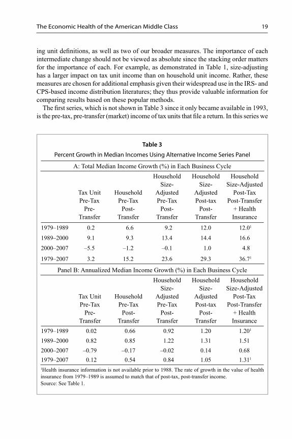
ing unit defi nitions, as well as two of our broader measures. The importance of each intermediate change should not be viewed as absolute since the stacking order matters for the importance of each. For example, as demonstrated in Table 1, size-adjusting has a larger impact on tax unit income than on household unit income. Rather, these measures are chosen for additional emphasis given their widespread use in the IRS- and CPS-based income distribution literatures; they thus provide valuable information for comparing results based on these popular methods.

The fi rst series, which is not shown in Table 3 since it only became available in 1993, is the pre-tax, pre-transfer (market) income of tax units that fi le a return. In this series we

Table 3

Percent Growth in Median Incomes Using Alternative Income Series Panel

A: Total Median Income Growth (%) in Each Business Cycle

Tax UnitPre-Tax

Pre-Transfer

HouseholdPre-Tax

Post-Transfer

Household Size-

AdjustedPre-Tax

Post-Transfer

Household Size-

AdjustedPost-tax

Post-Transfer

Household Size-Adjusted

Post-TaxPost-Transfer

+ Health Insurance

1979–1989 0.2 6.6 9.2 12.0 12.01

1989–2000 9.1 9.3 13.4 14.4 16.6

2000–2007 –5.5 –1.2 –0.1 1.0 4.8

1979–2007 3.2 15.2 23.6 29.3 36.71

Panel B: Annualized Median Income Growth (%) in Each Business Cycle

Tax UnitPre-Tax

Pre-Transfer

HouseholdPre-Tax

Post-Transfer

Household Size-

AdjustedPre-Tax

Post-Transfer

Household Size-

AdjustedPost-tax

Post-Transfer



+ Health Insurance

1979–1989 0.02 0.66 0.92 1.20 1.201

1989–2000 0.82 0.85 1.22 1.31 1.512000–2007 –0.79 –0.17 –0.02 0.14 0.681979–2007 0.12 0.54 0.84 1.05 1.311

1Health insurance information is not available prior to 1988. The rate of growth in the value of health insurance from 1979–1989 is assumed to match that of post-tax, post-transfer income.Source: See Table 1.


fi nd that median income fell by 2.7 percent in the 2000–2007 business cycle. Column 1 of Table 3 adds non-fi lers to the sample and reports their pre-tax, pre-transfer (market) income. This series most closely matches the Piketty and Saez (2003) tax unit sample. As can be seen from Panel A of Table 3, which presents this information as the total median income change over each business cycle, the median pre-tax, pre-transfer tax unit income of the entire population of tax units declined even more (5.5 percent) in the 2000–2007 business cycle.

Column 2 of Table 3 adds cash transfer income to the income defi nition and allows income to be shared across all members of a household rather than only within a tax unit. This series approximates the one the Census Bureau reports in their annual P-60 reports (DeNavas-Walt, Proctor, and Smith, 2008).14 When doing so, the real median income decline in the most recent business cycle shrinks from 5.5 percent (Column 1) to 1.2 percent, and the total median income growth over the past three business cycles quadruples from 3.2 percent (Column 1) to 15.2 percent.

Column 3 of Table 3 presents the most common income defi nition in the CPS-based inequality literature. This series, household size-adjusted, pre-tax, post-transfer income of the median person, rose by 23.6 percent over the three business cycles — well above the 3.2 percent increase for the median market income of tax units — and fell by only 0.1 percent in the 2000–2007 business cycle.

Columns 4 and 5 of Table 3 provide our series with broader income defi nitions than have traditionally been used in the literature. In Column 4, it is evident that including taxes and measuring post-tax, post-transfer, size-adjusted household cash income results in even faster median income growth. The gains in median net of tax income are most signifi cant over the 1980s business cycle but occurred over all three periods. Median income now rises by 29.3 percent over the entire period and by 1 percent between 2000 and 2007. Declines in tax rates over the past 30 years together combined with the rise of numerous credits have substantially positively impacted the median person’s net of tax income.

Finally, Column 5 of Table 3 adds the ex-ante value of employer and government provided health insurance to post-tax, post-transfer, size adjusted household income. Because these data are only available for the last two business cycles, we conserva-tively assume the ex-ante value of employer and government provided health insurance increased at the same rate as all other post-tax, post-transfer household income over the 1979–1989 business cycle. However, in both the 1989–2000 and 2000–2007 business cycles, accounting for health insurance payments further increased median income growth. While the 2.2 percent increase in median income growth from the increased value of health insurance was dwarfed by the overall 16.6 percent growth in income in the 1990s, accounting for the increased fraction of middle class compensation received

14 Our results do not exactly match the Census P-60 reports because the Census Bureau implements certain smoothing techniques (not included in the publicly provided data) to the CPS data prior to producing their report. Additionally, the Census P-60 report does not account for the 1992–1993 CPS trend break, since the report is designed as an annual snapshot rather than as a source of long-term trends.


in the form of health insurance in the 2000s results in median income growth increasing from 1 to 4.8 percent over 2000–2007. Hence at least part of the recent decline in the economic resources of the median American observed previously is the result of a shift in the way compensation and government transfers have been provided over the last two decades, as more compensation and transfers have come in the form of in-kind benefi ts.

Panel B of Table 3 reports the annualized median income growth in each business cycle to account for the different lengths of each business cycle. However, the pat-terns discussed above with respect to Panel A of Table 3 are the same. For instance, an anemic growth rate of 0.12 percent (Row 4, Column 1) in the market income of tax units over the entire period increases by 10 times to 1.31 percent (Row 4, Column 5) for the post-tax, post-transfer, household size-adjusted income including the ex-ante value of health insurance of persons. Likewise, an annual drop of 0.79 percent over the 2000–2007 business cycle in the market income of tax units (Column 1) is transformed into an annual increase of 0.68 percent in Column 5.

B. Quintile Incomes

While median income is a straightforward measure of how the average American is far-ing, it is also valuable to use a measure of the middle class that allows one to compare growth in the middle of the distribution to growth in the two tails.15 We do so below by comparing income trends for each quintile of the population.

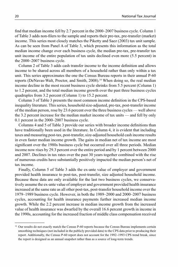
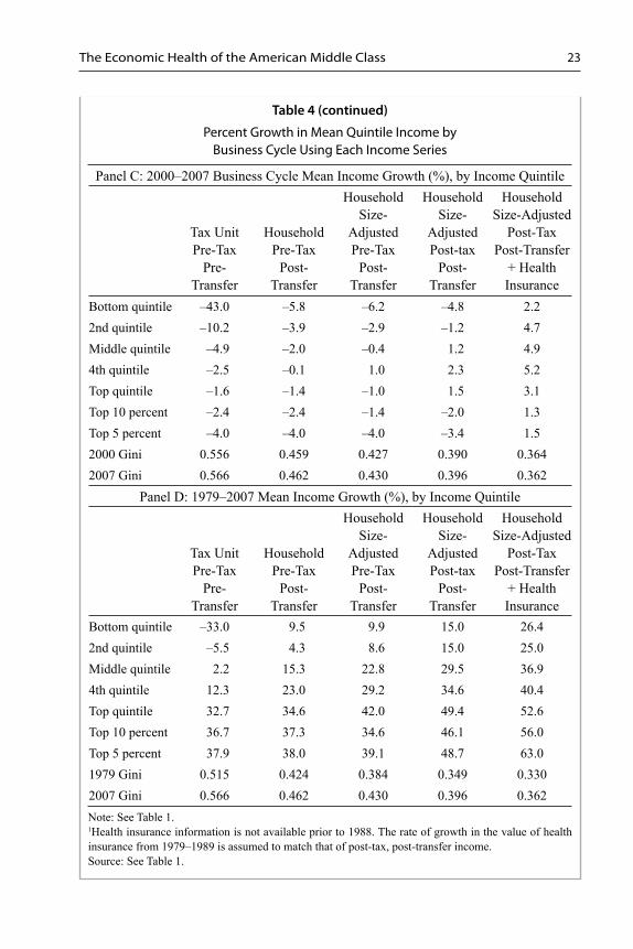
Table 4 shows the growth in mean income within each quintile of the distribution for each of our primary income series, holding the boundaries of the middle quintiles constant in real terms over each of the last three business cycles. We also provide the mean income of the top 10 and the top 5 percent of the distribution as well as the Gini coeffi cient for the entire distribution.

During the 1980s business cycle (Panel A), relative income growth across the fi ve quintiles of the distribution follows almost the same pattern in each income series. In each series income growth is more rapid for the third and fourth quintiles than for the fi rst two quintiles, and the top quintile of the distribution showed the fastest growth. Income growth in the top 5 percent of the distribution is the greatest of all. This result is consistent with earlier fi ndings that income inequality rose rapidly during the 1980s and that inequality growth occurred throughout the distribution (Piketty and Saez, 2003; Burkhauser et al., 2011).

Ostensibly the fi rst income series, which only considers market income, is an outlier across the fi ve measures. That is, using this fi rst series, it appears that over the 1980s the poorest two quintiles actually become poorer — i.e., they experienced negative growth. However, when in-cash government transfers and taxes are included and adjustments

15 An alternate approach to evaluating the extent to which economic gains are captured by the middle class is to compare median income growth in the CPS to GDP growth, productivity growth for non-farm busi-nesses, or mean per-capita income growth from the National Income and Products Accounts. For a fl avor of this approach, and a discussion of some of its challenges, see Gordon (2009).


Table 4

Percent Growth in Mean Quintile Income by Business Cycle Using Each Income Series

Panel A: 1979–1989 Business Cycle Mean Income Growth (%), by Income Quintile

Tax UnitPre-Tax

Pre-Transfer

HouseholdPre-Tax

Post-Transfer

Household Size-

AdjustedPre-Tax

Post-Transfer

Household Size-

AdjustedPost-tax

Post-Transfer



+ Health Insurance1

Bottom quintile –0.2 5.0 0.0 0.4 0.42nd quintile –5.0 0.2 –0.7 1.0 1.0Middle quintile 0.0 6.3 9.1 11.7 11.74th quintile 4.0 9.6 12.9 15.6 15.6Top quintile 17.6 19.7 23.4 28.1 28.1Top 10 percent 21.8 23.0 19.7 27.4 33.7Top 5 percent 25.6 26.3 27.2 32.0 39.51979 Gini 0.515 0.424 0.384 0.349 0.3301989 Gini 0.547 0.451 0.423 0.394 0.372

Panel B: 1989–2000 Business Cycle Mean Income Growth (%), by Income Quintile

Tax UnitPre-Tax

Pre-Transfer

HouseholdPre-Tax

Post-Transfer

Household Size-

AdjustedPre-Tax

Post-Transfer

Household Size-

AdjustedPost-tax

Post-Transfer



+ Health Insurance

Bottom quintile 17.8 10.6 17.2 20.4 23.22nd quintile 10.8 8.3 12.6 15.2 18.2Middle quintile 7.5 10.7 13.1 14.5 16.84th quintile 10.7 12.3 13.3 13.8 15.5Top quintile 14.7 14.0 16.2 14.8 15.5Top 10 percent 15.0 14.3 14.0 17.0 15.2Top 5 percent 14.4 13.8 13.9 16.6 15.11989 Gini 0.547 0.451 0.423 0.394 0.3722000 Gini 0.556 0.459 0.427 0.390 0.364


Table 4 (continued)

Percent Growth in Mean Quintile Income by Business Cycle Using Each Income Series

Panel C: 2000–2007 Business Cycle Mean Income Growth (%), by Income Quintile

Tax UnitPre-Tax

Pre-Transfer

HouseholdPre-Tax

Post-Transfer

Household Size-

AdjustedPre-Tax

Post-Transfer

Household Size-

AdjustedPost-tax

Post-Transfer



+ Health Insurance

Bottom quintile –43.0 –5.8 –6.2 –4.8 2.22nd quintile –10.2 –3.9 –2.9 –1.2 4.7Middle quintile –4.9 –2.0 –0.4 1.2 4.94th quintile –2.5 –0.1 1.0 2.3 5.2Top quintile –1.6 –1.4 –1.0 1.5 3.1Top 10 percent –2.4 –2.4 –1.4 –2.0 1.3Top 5 percent –4.0 –4.0 –4.0 –3.4 1.52000 Gini 0.556 0.459 0.427 0.390 0.3642007 Gini 0.566 0.462 0.430 0.396 0.362

Panel D: 1979–2007 Mean Income Growth (%), by Income Quintile

Tax UnitPre-Tax

Pre-Transfer

HouseholdPre-Tax

Post-Transfer

Household Size-

AdjustedPre-Tax

Post-Transfer

Household Size-

AdjustedPost-tax

Post-Transfer



+ Health Insurance

Bottom quintile –33.0 9.5 9.9 15.0 26.42nd quintile –5.5 4.3 8.6 15.0 25.0Middle quintile 2.2 15.3 22.8 29.5 36.94th quintile 12.3 23.0 29.2 34.6 40.4Top quintile 32.7 34.6 42.0 49.4 52.6Top 10 percent 36.7 37.3 34.6 46.1 56.0Top 5 percent 37.9 38.0 39.1 48.7 63.01979 Gini 0.515 0.424 0.384 0.349 0.3302007 Gini 0.566 0.462 0.430 0.396 0.362Note: See Table 1.1Health insurance information is not available prior to 1988. The rate of growth in the value of health insurance from 1979–1989 is assumed to match that of post-tax, post-transfer income.Source: See Table 1.


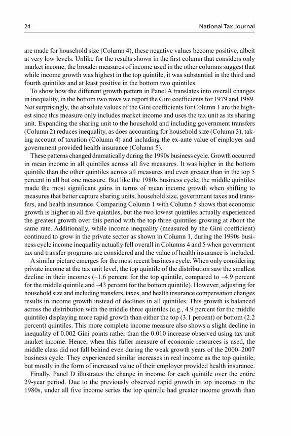
are made for household size (Column 4), these negative values become positive, albeit at very low levels. Unlike for the results shown in the fi rst column that considers only market income, the broader measures of income used in the other columns suggest that while income growth was highest in the top quintile, it was substantial in the third and fourth quintiles and at least positive in the bottom two quintiles.

To show how the different growth pattern in Panel A translates into overall changes in inequality, in the bottom two rows we report the Gini coeffi cients for 1979 and 1989. Not surprisingly, the absolute values of the Gini coeffi cients for Column 1 are the high-est since this measure only includes market income and uses the tax unit as its sharing unit. Expanding the sharing unit to the household and including government transfers (Column 2) reduces inequality, as does accounting for household size (Column 3), tak-ing account of taxation (Column 4) and including the ex-ante value of employer and government provided health insurance (Column 5).

These patterns changed dramatically during the 1990s business cycle. Growth occurred in mean income in all quintiles across all fi ve measures. It was higher in the bottom quintile than the other quintiles across all measures and even greater than in the top 5 percent in all but one measure. But like the 1980s business cycle, the middle quintiles made the most signifi cant gains in terms of mean income growth when shifting to measures that better capture sharing units, household size, government taxes and trans-fers, and health insurance. Comparing Column 1 with Column 5 shows that economic growth is higher in all fi ve quintiles, but the two lowest quintiles actually experienced the greatest growth over this period with the top three quintiles growing at about the same rate. Additionally, while income inequality (measured by the Gini coeffi cient) continued to grow in the private sector as shown in Column 1, during the 1990s busi-ness cycle income inequality actually fell overall in Columns 4 and 5 when government tax and transfer programs are considered and the value of health insurance is included.

A similar picture emerges for the most recent business cycle. When only considering private income at the tax unit level, the top quintile of the distribution saw the smallest decline in their incomes (–1.6 percent for the top quintile, compared to –4.9 percent for the middle quintile and –43 percent for the bottom quintile). However, adjusting for household size and including transfers, taxes, and health insurance compensation changes results in income growth instead of declines in all quintiles. This growth is balanced across the distribution with the middle three quintiles (e.g., 4.9 percent for the middle quintile) displaying more rapid growth than either the top (3.1 percent) or bottom (2.2 percent) quintiles. This more complete income measure also shows a slight decline in inequality of 0.002 Gini points rather than the 0.010 increase observed using tax unit market income. Hence, when this fuller measure of economic resources is used, the middle class did not fall behind even during the weak growth years of the 2000–2007 business cycle. They experienced similar increases in real income as the top quintile, but mostly in the form of increased value of their employer provided health insurance.

Finally, Panel D illustrates the change in income for each quintile over the entire 29-year period. Due to the previously observed rapid growth in top incomes in the 1980s, under all fi ve income series the top quintile had greater income growth than


the other four quintiles and the top 5 percent had the greatest income growth. Hence income inequality rose as measured by the Gini coeffi cient across all income series. But importantly, in contrast to tax unit market income measures of income where the bottom two quintiles get poorer and only the top quintile gets noticeably richer, each of the other series shows income growth throughout the distribution. Once taxes and health insurance are taken into account, each of the quintiles of the distribution is shown to have sizable growth over the 29-year period — with the slowest growth being a 26.4 percent increase in mean incomes for the bottom quintile of the distribution. Growth in the middle quintile is 36.9 percent, dramatically greater than their 2.2 percent growth in private market income when measured at the tax unit level. Income growth for the top quintile also increased to 52.6 percent, compared to the 32.7 percent growth in private market income of the tax unit. Despite this increased growth for the top quintile, how-ever, when using the broader income measure income growth is clearly more balanced throughout the distribution.

Given that income growth is more balanced throughout the distribution with the more comprehensive income measure, had Piketty and Saez (2003) used this income measure their observed growth in top income shares may have been less substantial. This is particularly true during the two business cycles since 1989 when the income growths for the top 5 and 10 percent of the income distribution were slower than that for the middle quintile with the most comprehensive income defi nition, but were faster than that of the middle quintile when using the cash market income of tax units defi nition.

Hence, these more inclusive measures of access to economic resources suggest that income inequality increased in the United States not because the rich got richer, the poor got poorer and the middle class stagnated, but because the rich got richer at a faster rate than the middle and poorer quintiles, primarily during the 1980s. Growth was substantial in all quintiles once the infl uence of government tax and transfer policy as well as the shift in compensation from wages to health insurance provided by employers and the shift to increased in-kind health insurance by government is recognized.

V. IMPACT ON PUBLIC POLICY DEBATES

Thus far, we have focused on how sensitive income measures are to changes in sharing unit and income defi nitions. However, these choices are also important when considering the impact of policy changes. The importance of income defi nitions for understanding policy debates should be self-evident. Taxes and transfers have a real impact on the well-being of the individuals paying the taxes and receiving the transfers, which is why proposed changes in these policies are often controversial. Since these components of incomes and expenses impact Americans’ available resources, we should include their effects in the statistics used to evaluate the success of public policies. By considering post-tax, post-transfer income including the value of health insurance, we can better capture the effect of program changes on people’s economic resources. Had we been able to include irregularly received income such as capital gains from investments or home sales, other non-cash government transfer income and employer compensation,


or imputed rents, median income growth likely would have been even stronger since many of these uncaptured sources increased over the past three business cycles.16

Less obvious, but similarly important, is how the choice of sharing unit infl uences the observed distribution of benefi ts of a given policy change. Although the distinction is often overlooked, this choice and the choice of whether to adjust for the size of the sharing unit can have profound effects on where individuals fall in the income distribu-tion and consequently on the distribution of the benefi ts of policy changes. While an individual’s location in the income distribution is positively correlated across sharing unit measures, this correlation is not perfect. Some low-income individuals in one distribution will be reported as having high-income in another depending on which sharing unit measure is employed.

Table 5 illustrates the extent to which the distributions of “not size-adjusted tax unit income” and “size-adjusted household income” differ — even when the income defi nition (post-tax, post-cash transfer including the ex-ante value of health insurance) is the same. If individuals in each of the quintiles in the tax unit distribution fell in the same quintiles of the household unit distribution, they would all lie on the diagonal of Table 5. This is not the case. Just 57 percent of individuals in the bottom quintile of the tax unit income distribution are also in the bottom quintile of the household income distribution (11.5 percent of the 20 percent of individuals in this quintile). The other

Table 5Comparing the Quintile Distributions of the Size-Adjusted Household Income

Distribution and Not Size-Adjusted Tax Unit Income Distribution (2007)

Quintile of Size-Adjusted Household Income

Quintile of Not Size-Adjusted Tax Unit IncomeBottom 2nd Middle 4th Top Total

Bottom 11.5 7.1 1.4 0.0 0.0 202nd 3.5 6.8 7.9 1.9 0.0 20Middle 2.2 3.3 6.5 7.4 0.6 204th 1.7 1.7 3.1 7.7 5.8 20Top 1.2 1.1 1.2 3.1 13.5 20Total 20 20 20 20 20 100

Notes: In both series the unit of analysis is the individual so each quintile contains 20 percent of individu-als in the population and income is measured using post-tax, post-transfer income including the ex-ante value of health insurance benefi ts.Source: See Table 1.

16 A fuller measure of resources would also include most or all of these sources which are not collected by the March CPS and thus are not analyzed here. For this reason, it may be benefi cial for the U.S. Census to more rigorously attempt to capture these income sources.


43 percent live in households with income above the bottom quintile. Overall, only 46 percent of all individuals are in the same quintiles of both distributions.

The different alignments of the distribution based on the sharing unit subsequently infl uence the perceived economic progressivity of public policies. To illustrate this general statement, we consider who benefi ts from the tax exemption for employer pro-vided health insurance. A similar analysis could be performed for any policy, including restructuring Social Security benefi ts, changing tax rates, or scaling back tax deduc-tions and credits.

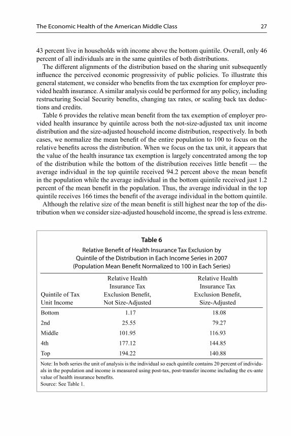
Table 6 provides the relative mean benefi t from the tax exemption of employer pro-vided health insurance by quintile across both the not-size-adjusted tax unit income distribution and the size-adjusted household income distribution, respectively. In both cases, we normalize the mean benefi t of the entire population to 100 to focus on the relative benefi ts across the distribution. When we focus on the tax unit, it appears that the value of the health insurance tax exemption is largely concentrated among the top of the distribution while the bottom of the distribution receives little benefi t — the average individual in the top quintile received 94.2 percent above the mean benefi t in the population while the average individual in the bottom quintile received just 1.2 percent of the mean benefi t in the population. Thus, the average individual in the top quintile receives 166 times the benefi t of the average individual in the bottom quintile.

Although the relative size of the mean benefi t is still highest near the top of the dis-tribution when we consider size-adjusted household income, the spread is less extreme.

Table 6 Relative Benefi t of Health Insurance Tax Exclusion by

Quintile of the Distribution in Each Income Series in 2007 (Population Mean Benefi t Normalized to 100 in Each Series)

Quintile of Tax Unit Income

Relative Health Insurance Tax

Exclusion Benefi t, Not Size-Adjusted

Relative Health Insurance Tax

Exclusion Benefi t, Size-Adjusted

Bottom 1.17 18.08

2nd 25.55 79.27

Middle 101.95 116.93

4th 177.12 144.85

Top 194.22 140.88

Note: In both series the unit of analysis is the individual so each quintile contains 20 percent of individu-als in the population and income is measured using post-tax, post-transfer income including the ex-ante value of health insurance benefi ts.Source: See Table 1.


Using this income series, the top quintile of the distribution receives 40.9 percent above the mean benefi t and those in the bottom quintile receive 18.1 percent. Thus, using this series, the mean benefi t going to the top quintile is less than 8 times that going to the bottom quintile. More generally, the values of the mean benefi t in the 2nd and the 3rd quintile also rise substantially and the size of the benefi t in the 4th quintile is now greater than the benefi t in the highest quintile.

Table 7 provides insight into why the spread of benefi ts differ across these series. In this table, individuals are divided into cells based on their location in the joint distribu-tion of not-size-adjusted tax unit income and size-adjusted household income. Each cell contains the mean benefi t from the health insurance tax exemption relative to both

Table 7 Comparing Relative Benefi ts of Health Insurance Tax Exclusion by

the Joint Quintile of the Size-Adjusted Household Income and Not Size-Adjusted Tax Unit Income Distributions in 2007

(Population Mean Benefi t is Normalized to 100 in Each Series)

Quintile of Size-Adjusted Household Income Bottom 2nd Middle 4th Top AllBottom HH: 3.2

TU: 1HH: 31.1TU: 35.7

HH: 76TU: 104.1

HH: N/ATU: N/A

HH: N/ATU: N/A

HH: 18.1TU: 20.3

2nd HH: 25.5TU: 1.3

HH: 31.7TU: 28.4

HH: 124.5TU: 145.6

HH: 162TU: 226.4

HH: 119.8TU: 225.9

HH: 79.3TU: 88.3

Middle HH: 63.1TU: 1.6

HH: 21.7TU: 10.4

HH: 107.4TU: 98.8

HH: 181.5TU: 220.7

HH: 154.8TU: 222.2

HH: 116.9TU: 122

4th HH: 108.9TU: 1.6

HH: 61.4TU: 11.8

HH: 36.7TU: 28.7

HH: 175.7TU: 170.1

HH: 195.4TU: 239.9

HH: 144.9TU: 141.4

Top HH: 128.7TU: 0.8

HH: 84.1TU: 8.9

HH: 53.1TU: 16.8

HH: 74.1TU: 60.5

HH: 169TU: 173.3

HH: 140.9TU: 128

All HH: 27.1TU: 1.2

HH: 62.2TU: 25.6

HH: 113.2TU: 101.9

HH: 144.6TU: 177.1

HH: 153TU: 194.2

Note: HH is the ratio of the mean benefi t to size-adjusted household income in the joint quintile to the mean benefi t to size-adjusted household income for the population. TU is the ratio of the mean benefi t to not-size-adjusted tax unit income in the joint quintile to the mean benefi t to not-size-adjusted tax unit income for the population. In both series the unit of analysis is the individual so each quintile contains 20 percent of individuals in the population.Source: See Table 1.

Quintile of (Not Size-Adjusted) Tax Unit Income


the population mean when using not-size-adjusted tax unit income and size-adjusted household income.

Among individuals along the diagonal where the quintile of both income distribu-tions is the same, the ratio of mean quintile benefi t to mean population benefi t is similar for both series. This is not the case for individuals in quintiles off the diagonal (i.e., those who switch quintiles depending on which unit of measurement is employed). Individuals below the diagonal are in a higher quintile for household income than they are for tax unit income. This can occur, for instance, when low-income grown children live with their higher income parents. For these individuals, the relative mean benefi ts from tax-deductible employer provided health insurance observed for household units exceeds that observed for tax units. This is particularly evident among individuals in the bottom quintile of tax units, where almost no benefi ts are observed at the tax unit level but substantial benefi ts may be observed at the household level. Thus, by missing the benefi ts for these individuals, using tax units exacerbates the perceived disparity in the tax advantage of exempting employer provided health insurance across the income distribution. In contrast, above the diagonal there is less of a distinction between the two series as even individuals in the bottom quintiles of the household income distri-bution are still receiving benefi ts from the income exclusion. Therefore, an exclusive focus on the tax unit obscures the fact that within low income quintiles there is a range of benefi ts and some households at the bottom of the distribution do, in fact, receive substantial benefi ts from this policy.

VI. CONCLUSIONS

Much of the previous research on income and its distribution is based on the types of income captured in the data and the sharing unit over which it was collected, without fully considering the implications of those choices. In this paper, we demonstrate that such choices can substantially change the view of how the average American has fared over the past three business cycles (1979–2007) and who benefi ts from public policy choices going forward. When using the most restrictive income defi nition — pre-tax, pre-transfer tax unit cash (market) income — the resources available to the middle class have stagnated over the past three business cycles. In contrast, once broadening the income defi nition to post-tax, post-transfer, size-adjusted household cash income, middle class Americans are found to have made substantial gains, and these increases are even larger when including non-cash income such as the ex-ante value of health insurance. Additionally, as we demonstrate using the example of the benefi ts of the tax exclusion of employer provided health insurance, these measurement decisions impact the extent to which we view policy benefi ts as skewed towards the top or bottom of the income distribution or view them as distributed more widely to individuals of all incomes.

So which income series is superior? This depends on the research question. For researchers interested in how middle class Americans are compensated for their time in the labor market, for example, it is more appropriate to use pre-tax, pre-transfer


(market) income, although even here researchers who ignore the dramatic increase in the ex-ante value of employer health insurance will understate the returns to work in the United States and disproportionately do so for workers in middle class households. However, for those interested in the overall economic resources available to individuals, it is more appropriate to consider income defi ned as broadly as possible, consistent with the traditional Haig-Simons measure of comprehensive income as the best measure of ability to pay tax.

In most cases, it is more important to know how a given policy impacts people arrayed by available resources within their sharing unit than how that policy impacts their market income. In such cases, researchers should broaden the defi nition of income to include taxes and non-cash benefi ts. This will more accurately refl ect the total fi nancial resources available to individuals. Additionally, they should do so across households rather than tax units and adjust for the number of people in those households. As we have demonstrated, doing so provides a markedly different picture of how middle class Americans have fared over the past several decades.

ACKNOWLEDGEMENTS AND DISCLAIMERS

We thank Jennifer Tennant and Abigail Kelly-Smith for their helpful comments and suggestions and Sean Lyons for research assistance with some of the data used in this paper. The views in this paper are those of the authors and should not be attributed to the staff of the Joint Committee on Taxation or any Member of Congress.

REFERENCES

Atkinson, Anthony B., and Andrea Brandolini, 2001. “Promises and Pitfalls in the Use of Sec-ondary Data Sets: Income Inequality in OECD Countries as a Case Study.” Journal of Economic Literature 39 (3), 771–799.

Atkinson, Anthony B., Thomas Piketty, and Emmanuel Saez, 2011. “Top Incomes in the Long Run of History.” Journal of Economic Literature 49 (1), 3–71.

Auten, Gerald, and Geoffrey Gee, 2009. “Income Mobility in the United States: New Evidence from Income Tax Data.” National Tax Journal 62 (2), 301–328.

Buhmann, Brigitte, Lee Rainwater, Guenther Schmaus, and Timothy M. Smeeding, 1988. “Equivalence Scales, Well-being, Inequality, and Poverty: Sensitivity Estimates Across Ten Countries Using the Luxembourg Income Study (LIS) Database.” Review of Income and Wealth 34 (2), 115–142.

Burkhauser, Richard V., Shuaizhang Feng, Stephen P. Jenkins, and Jeff Larrimore, forthcoming. “Recent Trends in Top Income Shares in the USA: Reconciling Estimates from March CPS and IRS Tax Return Data.” Review of Economics and Statistics.

Burkhauser, Richard V., Shuaizhang Feng, Stephen P. Jenkins, and Jeff Larrimore, 2011. “Trends in United States Income Inequality Using the March Current Population Survey: The Importance of Controlling for Censoring.” Journal of Economic Inequality 9 (3), 393–415.


Burkhauser, Richard V., and Jeff Larrimore, 2011. “How Changes in Employment, Earnings, and Public Transfers Make the First Two Years of the Great Recession (2007–2009) Different from Previous Recessions and Why It Matters for Longer Term Trends.” Russell Sage Foundation US2010 Project Research Brief. Russell Sage Foundation, New York, NY, http://www.s4.brown.edu/us2010/Data/Report/report3.pdf.

Burkhauser, Richard V., and Kosali I. Simon, 2010. “The Importance of Health Insurance in Measuring Levels and Trends in United States Income Inequality.” NBER Working Paper No. 15811. National Bureau of Economic Research, Cambridge, MA.

Chung, Wankyo, 2003. “Fringe Benefi ts and Inequality in the Labor Market.” Economic Inquiry 41 (3), 517–529.

Cutler, David M., 2004. Your Money or Your Life: Strong Medicine for America’s Healthcare System. Oxford University Press, New York, NY.

DeNavas-Walt, Carmen, Bernadette D. Proctor, and Jessica C. Smith, 2008. Income, Poverty, and Health Insurance Coverage in the United States: 2007. Current Population Reports P60–235. U.S. Census Bureau, Washington, DC.

d’Ercole, Marco Mira, and Michael Förster, forthcoming. “The OECD Approach to Measuring Income Distribution and Poverty: Strengths, Limits and Statistical Issues.” In Besharov, Douglas J., and Kenneth A. Couch (eds.), European Measures of Income and Poverty: Lessons for the U.S. Oxford University Press, New York, NY.

Elmendorf, Douglas W., Jason Furman, William G. Gale, and Benjamin H. Harris, 2008. “Distri-butional Effects of the 2001 and 2003 Tax Cuts: How Do Financing and Behavioral Responses Matter?” National Tax Journal 61 (3), 365–380.

Feenberg, Daniel, and Elisabeth Coutts, 1993. “An Introduction to the TAXSIM Model.” Journal of Policy Analysis and Management 12 (1), 189–194.

Goldman, David, 2008. “Work Harder, Take Home Less.” CNN.com, August 28, http://money.cnn.com/2008/08/27/news/economy/state_of_working_america/index.htm.

Gordon, Robert J., 2009. “Misperception About the Magnitude and Timing of Changes in American Income Inequality.” NBER Working Paper No. 15351. National Bureau of Economic Research, Cambridge, MA.

Gottschalk, Peter, and Sheldon Danziger, 2005. “Inequality of Wage Rates, Earnings and Fam-ily Income in the United States, 1975–2002.” Review of Income and Wealth 51 (2), 231–254.

Johnson, David Cay, 2007. “Income Gap is Widening Data Shows.” The New York Times, March 29, C1.

Jones, Arthur F., Jr., and Daniel H. Weinberg, 2000. “The Changing Shape of the Nation’s Income Distribution.” Current Population Reports, P60-204. U.S. Census Bureau, Washington, DC.

Karoly, Lynn A., 1994. “Trends in Income Inequality: The Impact of, and Implications for, Tax Policy.” In Slemrod, Joel B. (ed.), Tax Progressivity and Income Inequality, 95–129. Cambridge University Press, New York, NY.


Lahart, Justin, and Kelly Evans, 2008. “Trapped in the Middle.” The Wall Street Journal, April 19, A1.

Larrimore, Jeff, Richard V. Burkhauser, Shuaizhang Feng, and Laura Zayatz, 2008. “Consistent Cell Means for Topcoded Incomes in the Public Use March CPS (1976–2007).” Journal of Economic and Social Measurement 33 (2–3), 89–128.

Leonhardt, David, 2008. “For Many a Boom That Wasn’t.” The New York Times, April 9, C1.

Meyer, Bruce D., and James X. Sullivan, 2009a. “Consumption and Income Inequality in the U.S.: 1960–2008.” Paper presented at Economic Crisis, Rising Unemployment and Policy Responses: What Does It Mean for the Income Distribution, February 8–9, sponsored by the Institute for the Study of Labor and the Organization for Economic Co-operation and Development. Paris, France.

Meyer, Bruce D., and James X. Sullivan, 2009b. “Five Decades of Consumption and Income Pov-erty.” NBER Working Paper No. 14827. National Bureau of Economic Research, Cambridge, MA.

Obama, Barack, 2009. Memorandum for the Heads of Executive Departments and Agencies: White House Task Force on Middle-Class Working Families. The White House, Washington, DC, http://www.whitehouse.gov/the_press_offi ce/memorandum_for_the_heads_of_executive_departments_and_agencies/.

Pierce, Brooks, 2001. “Compensation Inequality.” Quarterly Journal of Economics 116 (4), 1493–1525.

Pierce, Brooks, 2010. “Recent Trends in Compensation Inequality.” In Abraham, Katharine G., James R. Spletzer, and Michael Harper (eds.), Labor in the New Economy, 63–98. University of Chicago Press, Chicago, IL.

Piketty, Thomas, and Emmanuel Saez, 2003. “Income Inequality in the United States, 1913–1998.” Quarterly Journal of Economics 118 (1), 1–39.

Piketty, Thomas, and Emmanuel Saez, 2007. “How the Income Share of Top 1% of Families has Increased Dramatically.” The Wall Street Journal, January 11, B6.

Ruggles, Patricia, 1990. Drawing the Line: Alternative Poverty Measures and Their Implication for Public Policy. Urban Institute Press, Washington, DC.

Ryscavage Paul, 1995. “A Surge in Growing Income Inequality?” Monthly Labor Review 118 (8), 51–61.

Saez, Emmanuel, 2009. “Striking it Richer: The Evolution of Top Incomes in the United States.” Working Paper. University of California, Berkeley, CA.

Smeeding, Timothy, Lee Rainwater, and Gary Burtless, 2001. “United States Poverty in a Cross-National Context.” FOCUS Institute for Research on Poverty 21 (3), 50–54.

Stewart, Kenneth J., and Stephen B. Reed, 1999. “CPI Research Series Using Current Methods, 1978–98.” Monthly Labor Review 122 (6), 29–38.

"a 'second opinion' on the economic health of the american ... · a “second...

Documents