a semi-discrete new twist on the petitot theory

HYPOELLIPTIC DIFFUSION AND HUMAN VISION:

A SEMI-DISCRETE NEW TWIST ON THE PETITOT THEORY

UGO BOSCAIN, ROMAN CHERTOVSKIH, JEAN-PAUL GAUTHIER,AND ALEXEY REMIZOV

Abstract. This paper is devoted to present an algorithm implementing thetheory of neurogeometry of vision, described by Jean Petitot in his book. We

propose a new ingredient, namely working on the group of translations and

discrete rotations SE(2, N). We focus on the theoretical and numerical aspectsof integration of an hypoelliptic diffusion equation on this group. Our main

tool is the generalized Fourier transform. We provide a complete numerical

algorithm, fully parallellizable. The main objective is the validation of theneurobiological model.

Keywords: neurogeometry, hypoelliptic diffusion, sub-Riemannian geometry,generalized Fourier transform

1. Introduction

In his beautiful book [36], Jean Petitot describes a sub-Riemannian model of theVisual cortex V1.

The main idea goes back to the paper by Hubel an Wiesel in 1959 (Nobel prizein 1981) [27] who showed that in the visual cortex V1, there are groups of neuronsthat are sensitive to position and directions1 with connections between them thatare activated by the image. The key fact is that the system of connections betweenneurons, which is called the functional architecture of V1, preferentially connectsneurons detecting alignements. This is the so-called pinwheels structure of V1.

Therefore it is likely that V1 lifts the images f(x, y) (i.e., functions of two positionvariables x, y in the plane R2 of the image) to functions over the projective tangentbundle PTR2. This bundle has as base R2 and as fiber over the point (x, y) the setof directions of straight lines lying on the plane and passing through (x, y).

Consider for instance the simplest case in which the image is a smooth curveR 3 t→ (x(t), y(t)) ∈ R2. Lifting this curve to PTR2 means to add a new variableθ(t) that is the angle of the vector (x(t), y(t)).

Since we are obliged at some point to go to certain stochastic considerations,it is convenient to write this lift in the following “control form”. We say that

Date: January 30, 2013.

2000 Mathematics Subject Classification. Primary 93-04; Secondary 93C10, 93C20.Key words and phrases. Sub-Riemannian geometry, image reconstruction, hypoelliptic

diffusion.1 Geometers call “directions” (angles modulo π) what neurophysiologists call “orientations”.

1

arX

iv:1

304.

2062

v2 [

mat

h.A

P] 9

Jun

201

3

2 U. BOSCAIN, R. CHERTOVSKIH, J.-P. GAUTHIER, AND A. REMIZOV

(x(·), y(·), θ(·)) is the lift of the curve (x(·), y(·)) if there exist two functions u(·)and v(·) (called controls) such that2

(1.1)

( x(t)y(t)

θ(t)

)= u(t)

(cos(θ(t))sin(θ(t))

0

)+ v(t)

(001

).

Here the control u(t) plays the role of the modulus of the planar vector (x(t), y(t)),but can take positive and negative values since the angle θ(t) is defined modulo π.The control v(t) is just the derivative of θ(t).

Remark 1. The vector distribution N(x, y, θ) := span {F (x, y, θ), G(x, y, θ)}, where3

F (x, y, θ) =

( cos(θ)sin(θ)

0

), G(x, y, θ) =

( 001

),

endows PTR2 with the structure of a contact manifold. Indeed N is completely non-integrable (in the Frobenius sense) since F and G satisfy the Hormander condition:span {F,G, [F,G]} = TqPTR2 for each q ∈ PTR2.

In the model described by Petitot, when a curve is partially interrupted, it isreconstructed by minimizing the energy necessary to activate the regions of thevisual cortex that are not excited by the image. Roughly speaking, neurons of V1are grouped into orientation columns, each of them being sensitive to visual stimuliat a given point of the retina and for a given direction on it. Orientation columnsare themselves grouped into hypercolumns, each of them being sensitive to stimuliat a given point with any direction (see Figure 1).

In the visual cortex there are two types of connections: the vertical connectionsamong orientation columns in the same hypercolumn, and the horizontal connec-tions among orientation columns belonging to different hypercolumns and sensitiveto the same orientation. For an orientation column it is easy to activate anotherorientation column which is a “first neighbor” either by horizontal or by verticalconnections.

In the model described by Petitot the energy necessary to activate a path [0, T ] 3t 7→ (x(t), y(t), θ(t)) is given by∫ T

0

(x(t)2 + y(t)2 +

1

αθ(t)2

)dt =

∫ T

0

(u(t)2 +

1

αv(t)2

)dt.

The term x(t)2 + y(t)2 is proportional to the energy necessary to activate horizontal

connections, while the term θ(t)2 is proportional to the energy necessary to activatevertical connections. The parameter α > 0 is a relative weight.

2 Which curves can be lifted with this procedure is an interesting question (see for instance

[9]). In this paper we are not focused on this problem. Let us just observe that a planar curvehaving a cusp (as for instance [−1, 1] 3 t 7→ (t3, t2)) has a smooth lift.

3Notice that the definition of vector field F is not global over PTR2 since it is not continuousat θ = π ∼ 0: the distribution N is not trivializable and a correct definition of it would requiretwo charts. However, for sake of simplicity, we proceed with a single chart with some abuse of

notation. Notice, however, that if we lift the problem to the group SE(2), which is a doublecovering of PTR2, the structure becomes trivializable and the definition of F becomes global. Wedo this often along the paper.

HYPOELLIPTIC DIFFUSION AND HUMAN VISION 3

(horizontal)curve

visual cortex V1

activ

atio

n

activ

atio

n

orientation columns

Plane of the image

connections among orientation columns in the same hypercolumn(vertical)

hypercolumns

connections among orientation columns belonging to different hypercolumnsand sensible to the same orientation

Figure 1. The structure of V1

To conclude, in V1, the problem of reconstructing a curve interrupted betweenthe boundary conditions (x0, y0, θ0) and (x1, y1, θ1) becomes the optimal controlproblem4 ( x(t)

y(t)

θ(t)

)= uF (x, y, θ) + vG(x, y, θ),

∫ T

0

(u(t)2 +

1

αv(t)2

)dt→ min,

(x(0), y(0), θ(0)) = (x0, y0, θ0), (x(T ), y(T ), θ(T )) = (x1, y1, θ1).(1.2)

Finding the solution to this optimal control problem can be seen as the problemof finding the minimizing geodesic for the sub-Riemannian structure over PTR2

defined as follows: The distribution is N and the metric gα over N is the oneobtained by claiming that the vector fields F and

√αG form an orthonormal frame.

By construction, this sub-Riemannian manifold is invariant under the action of thegroup of rototranslations of the plane SE(2). Indeed, {N, gα}α∈]0,∞[ are all the sub-

Riemannian structures over PTR2 which are invariant under the action of SE(2).See for instance [2].

Remark 2. From the theoretical point of view, the weight parameter α is irrelevant:for any α > 0 there exists a homothety of the (x, y)-plane that maps geodesics ofthe metric with the weight parameter α to those of the metric with α = 1. Forthis reason, in all theoretical considerations we fix α = 1. However its role will beimportant in our inpaiting algorithms (see Section 2.3).

4 Here the time T should be fixed, but changing T changes only the parameterization of thesolutions. For the same reasons as in Riemannian geometry, minimizer of the sub-Riemannian en-

ergy∫ T0

(u(t)2 + 1

αv(t)2

)dt are minimizers of the sub-Riemannian length

∫ T0

√u(t)2 + 1

αv(t)2 dt.


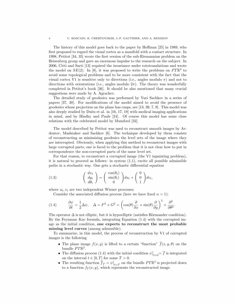
The history of this model goes back to the paper by Hoffman [25] in 1989, whofirst proposed to regard the visual cortex as a manifold with a contact structure. In1998, Petitot [34, 35] wrote the first version of the sub-Riemannian problem on theHeisenberg group and gave an enormous impulse to the research on the subject. In2006, Citti and Sarti [13] required the invariance under rototranslations and wrotethe model on SE(2). In [8], it was proposed to write the problems on PTR2 toavoid some topological problems and to be more consistent with the fact that thevisual cortex V1 is sensitive only to directions (i.e., angles modulo π) and not todirections with orientations (i.e., angles modulo 2π). The theory was wonderfullycompleted in Petitot’s book [36]. It should be also mentioned that many crucialsuggestions were made by A. Agrachev.

The detailed study of geodesics was performed by Yuri Sachkov in a series ofpapers [37, 38]. For modifications of the model aimed to avoid the presence ofgeodesics whose projection on the plane has cusps, see [13, 39, 7, 9]. This model wasalso deeply studied by Duits et al. in [16, 17, 18] with medical imaging applicationsin mind, and by Hladky and Pauls [24]. Of course this model has some closerelations with the celebrated model by Mumford [32].

The model described by Petitot was used to reconstruct smooth images by Ar-dentov, Mashtakov and Sachkov [6]. The technique developed by them consistsof reconstructing as minimizing geodesics the level sets of the image where theyare interrupted. Obviously, when applying this method to reconstruct images withlarge corrupted parts, one is faced to the problem that it is not clear how to put incorrespondence the non-corrupted parts of the same level set.

For that reason, to reconstruct a corrupted image (the V1 inpainting problem),it is natural to proceed as follows: in system (1.1), excite all possible admissiblepaths in a stochastic way. One gets a stochastic differential equation

(1.3)

( dxtdytdθt

)=

( cos(θt)sin(θt)

0

)dut +

( 001

)dvt,

where ut, vt are two independent Wiener processes.Consider the associated diffusion process (here we have fixed α = 1):

(1.4)∂ψ

∂t=

1

2∆ψ, ∆ = F 2 +G2 =

(cos(θ)

∂

∂x+ sin(θ)

∂

∂y

)2

+∂2

∂θ2.

The operator ∆ is not elliptic, but it is hypoelliptic (satisfies Hormander condition).By the Feynman–Kac formula, integrating Equation (1.4) with the corrupted im-age as the initial condition, one expects to reconstruct the most probablemissing level curves (among admissible).

To summarize, in this model, the process of reconstruction by V1 of corruptedimages is the following

• The plane image f(x, y) is lifted to a certain “function” f(x, y, θ) on thebundle PTR2.• The diffusion process (1.4) with the initial condition ψ

∣∣t=0

= f is integrated

on the interval t ∈ [0, T ] for some T > 0.• The resulting function fT = ψ

∣∣t=T

on the bundle PTR2 is projected down

to a function fT (x, y), which represents the reconstructed image.


The lifting procedure should be as follows: the image is assumed to be a smooth5

function f(x, y). Then, it can be naturally lifted to a surface S in PTR2 by liftingits level curves. At a point (x, y, θ) we would like to set f(x, y, θ) = f(x, y) if(x, y, θ) ∈ S and f(x, y, θ) = 0 elsewhere. But this would be nonsense since S haszero measure in PTR2. Hence, f(x, y) is lifted to a distribution f(x, y, θ), supportedin S, and weighted by f(x, y). We refer to [8] for details.

The idea of modeling the process of reconstruction of images in V1 as an hy-poelliptic diffusion was presented first in [13] and was implemented in details withsome slight modifications and different purposes in [39, 8, 17, 18]. A clever variantto the lifting process was proposed in [17, 18].

It turns out that although looking rather simple, Equation (1.4) is not that easyto integrate numerically. In particular, the multiscale sub-Riemannian effects arehidden inside. (The numerical literature for PDEs in sub-Riemannian geometryappears to be very scarce.)

For the equation (1.4) it is possible to compute the associated heat kernel, see[3] and [16, 17]; however, the direct use of the kernel quickly appears to be not verytractable. Moreover, the numerical integration starts to be a rather large problem,due to the number of points/angles in a reasonable image. To get an idea of thesize of the full space-discretization of the problem, see Remark 5 below.

For these reasons, only very recently, some promising results about inpaintingusing hypoelliptic diffusion were obtained in [8]. In that paper a sophisticatedalgorithm based upon the generalized Fourier transform on the group SE(2) wasused.

In this paper, we introduce a new ingredient, namely we conjecture the following:

• the visual cortex can detect a finite (small) number of directions only.

This conjecture is based on the observation of the organization of the visualcortex in pinwheels. The planar and the angular degrees of freedom cannot betreated in the same way. We conjecture that there are topological constraints thatprevent the possibility of detecting a continuum of directions even when sendingthe distance between pinwheels to zero.

In this paper we are not going to justify this conjecture. Rather, we concentrateon the effect of this conjecture on the mathematical model and on our ability tointegrate the hypoelliptic diffusion equation.

The main purpose of this paper is to write an inpainting algorithm which makesuse of the group of continuous translations and discrete rotation SE(2, N). Thisgroup has very special features: it is maximally almost periodic, and all its unitaryirreducible representations are finite dimensional. Moreover, for this group the heatkernel can be written in a very simple form (see Sections 2.2.2 and 2.2.3).

In the following, when using the group SE(2, N) instead than SE(2) for inpait-ing, we speak of the “semi-discrete variant” to the Petitot theory.

It turns out that we were led to rather abstract considerations, to get at the enda quite simple algorithm, massively parallelizable. This aspect of parallelizabilityseems to fit with the structure of the visual cortex V1, which is thought to make alot of parallel computations.

5In fact, it is known by biologists that a certain smoothing procedure is already applied at thelevel of the retina [15, 30, 33].


The paper is organized as follows: in the next section 2, we discuss some prop-erties of the group SE(2) and its discrete avatars, together with a discrete versionof the hypoelliptic diffusion (1.4).

Section 3 presents our main ideas and shows a first algorithm, which is notsuitable in our case, mostly for two reasons:

• The “distributional” nature of lifted images (initial conditions).• Compared to our final algorithm, it does not present the same capability

to treat in a different way the corrupted and non-corrupted parts of theimage (see Section 5).

However, this approach could certainly be interesting for more smooth initial con-ditions.

Section 4 presents our final algorithm that, due to the abstract structure ofthe groups under consideration, is massively parallel: It reduces the problem to anumber of problems of integration of linear differential equations in low dimension,completely decoupled.

Section 5 presents some heuristic improvements of the algorithm in the casewhere we can distinguish between the corrupted and non-corrupted parts of theimage.

In Appendix A, we present a series of results of reconstruction with high corrup-tion rates and the table of all parameters used for the reconstruction procedures.These parameters include: the time of diffusion, the weight α, and other parame-ters that are used to “tune” the action of the diffusion on the corrupted and noncorrupted points.

Finally, Appendix B is devoted to basic theoretical concepts and to certain tech-nical computations.

We do not pretend that our results are better than the inpainting algorithmsexisting today. We just claim that they really seem to validate the theory describedby Jean Petitot and our semi-discrete variant. Moreover we emphasize the globalcharacter of the basic algorithm.

We do not discuss the final step of the algorithm (projection) here. There areat least two obvious possibilities: projecting by taking either the maximum, or theaverage, over angles. Numerous experiments show that the projection made by themaximum provides better results.

2. The Operators and the groups under consideration

2.1. Groups. We advise the uninitiated reader to start with our paper [3] and tohave a look to Appendix B at the end of this paper.

2.1.1. The group of Motions SE(2). The group law over the Lie group SE(2) hasmultiplication law (X2, θ2) · (X1, θ1) = (X2 +Rθ2X1, θ1 + θ2), where

X =

(xy

), Rθ =

(cos(θ) sin(θ)− sin(θ) cos(θ)

),

Rθ is the rotation of angle θ in the X-plane.The (strongly continuous) unitary irreducible representations of SE(2) are well

known. However for analogy with the next section, we need to recall basic facts.For a survey, see [40, 41].


As representations of a semi-direct product, they can be obtained by usingMackey’s imprimitivity theorem, and therefore, they are parametrized by the orbitsof the (contragredient) action of rotations on theX-plane, i.e., they are parametrizedby the half lines passing through the origin. Additionally, corresponding to the ori-gin, there are the characters of the rotation group S1 that do not count in thesupport of the Plancherel’s measure. Finally, the representation χλ correspondingto the circle of radius λ acts over L2(S1), and is given by

[χλ(X, θ) · ϕ](u) = ei〈vλ,RuX〉ϕ(u+ θ),

where vλ is a vector of length λ in R2 and 〈·, ·〉 denotes the standard Euclideanscalar product over R2.

Note that SE(2) is far from being maximally almost periodic, since all its finitedimensional unitary irreducible representations are given by the characters of S1

only.Let us also recall [3, 8, 16, 17] that the sub-Riemannian heat kernel on SE(2),

corresponding to the hypoelliptic Laplacian 12∆ defined in (1.4) is given by6

(2.1) Pt(X, θ) =1

2

+∞∫0

(+∞∑n=0

eaλnt

⟨cen

(θ,λ2

4

), χλ(X, θ) cen

(θ,λ2

4

)⟩+

+∞∑n=0

ebλnt

⟨sen

(θ,λ2

4

), χλ(X, θ) sen

(θ,λ2

4

)⟩λdλ,

where the functions sen and cen are the 2π-periodic Mathieu sines and cosines, and

aλn = −λ2

4 − an(λ2

4

), bλn = −λ

2

4 − bn(λ2

4

), with an, bn, the characteristic values for

the Mathieu equation.Then the solution of the diffusion equation (1.4) with the initial condition ψ

∣∣t=0

=ψ0 is given by the right-convolution formula:(2.2)

ψ(t,X, θ) = et∆ψ0(X, θ) = ψ0(X, θ) ∗ Pt(X, θ)=

∫SE(2)

ψ0(g)Pt(g−1 · (X, θ)

)dg,

where g ∈ SE(2) and dg is the Haar measure: dg = dxdydθ. Unfortunately, inpractice formula (2.2) is not very tractable, for several reasons (in particular, dueto the slow convergence and the difficulty to find good computer implementationsof Mathieu functions).

2.1.2. The group of discrete motions SE(2, N). In the next section, a discrete-angleversion of the above diffusion equation will appear naturally. It corresponds to thegroup of motions SE(2) restricted to rotations with angles 2kπ

N . This group isdenoted by SE(2, N). It has very special features: it is maximally almost periodic,and all its unitary irreducible representations are finite dimensional (it is a Mooregroup, see [23] for details), although it is not compact. This follows in particularfrom [19, 16.5.3, page 304]: it is the semi-direct product of a compact subgroup K =Z/NZ, and a normal subgroup V isomorphic to R2, each element of V commutingwith the connected component of the identity (which in this case is V itself). Tosimplify, we set Rk = R 2kπ

N.

6in this formula α = 1


Besides the characters of K, the representations coming in the support of the

Plancherel measure are parametrized by (λ, ν) ∈ R+∗ ×[0, 2π

N [ = SE(2, N), the dual7

of SE(2, N). They act on CN and are given by

(2.3) χλ,ν(X, r) = diagk(ei〈Vλ,ν ,RkX〉

)Sr,

where diagk(ei〈Vλ,ν ,RkX〉

)is the diagonal matrix with diagonal elements ei〈Vλ,ν ,RkX〉,

Vλ,ν = (λ cos(ν), λ sin(ν)), k = 1, . . . , N , and S is the shift matrix over CN (i.e.,Sek = ek+1 for k = 1, . . . , N − 1, and SeN = e1).

2.2. The semi-discrete diffusion operator.

2.2.1. Semi-discrete versus continuous. Firstly, we show that a certain semi-discrete(discretization with respect to the angle) model of the diffusion is compatible withthe limit continuous model. For the considerations in this section, one may refer tothe paper [5].

The diffusion equation (1.4) comes from the stochastic differential equation (1.3),where ut, vt are two independent standard Wiener processes. It is the associatedFokker-Planck (or Kolmogorov forward) equation to (1.3).

From the image processing point of view, integrating the diffusion is equivalentto excite all possible admissible paths, in a stochastic way.

In fact, in the real structure of the V1 cortex, a finite (small) number ofangles only is taken into account. Here this number is denoted by N .

Therefore, it is natural to consider the following stochastic process with jumpsevidently connected with the stochastic equation (1.3):

(2.4) dzt =

(dxtdyt

)=

(cos(θt)sin(θt)

)dvt,

in which θt is a jump process. Set ΛN = (λi,j), i, j = 0, . . . , N − 1, where

λi,j = limt→0

P [θt = ej |θ0 = ei]

tfor i 6= j, λj,j = −

∑i6=j

λi,j .

The matrix ΛN is the infinitesimal generator of the jump process.We assume Markov processes, where the law of the first jump time is exponential,

with parameter β > 0 (that will be specified later on). The jump has probability12 on both sides. Then we get a Poisson process, and the probability of k jumpsbetween 0 and t is

P [k jumps] =(βt)k

k!e−βt.

So that:

P [θt = ei±1|θ0 = ei] =1

2

(βt+ kt2 + o(t2)

)e−βt,

P [θt = ei±2|θ0 = ei] =1

4

(1

2β2t2 + o(t2)

)e−βt,

P [θt = ei±n|θ0 = ei] = O(tn)e−βt, n = 2, 3, . . . ,

with the convention that ei is modulo N .

7 The natural “dual topology” of SE(2, N) is that of a cone, that consists of considering

R+∗ × [0, 2π

N] and identifying (λ, 0) with (λ, 2π

N).


Hence λi,i±1 = 12β and λi,i = −β. All other elements of the matrix ΛN are equal

to zero. Then, the infinitesimal generator of the semi-group associated with thestochastic process (zt, θt) is of the form:

(2.5) LNΨ(z, ei) = (AΨ)i(z) + (ΛNΨ(z, ei))i,

where Ψj(z) = Ψ(z, ej), z = (x, y), and

(2.6) (AΨ)i(z) = AΨ(z, ei) =1

2

(cos(ei)

∂

∂x+ sin(ei)

∂

∂y

)2

Ψ(z, ei),

(2.7) (ΛNΨ(z, ei))i =

n−1∑j=0

λi,jΨj(z) =β

2

(Ψi−1(z)− 2Ψi(z) + Ψi+1(z)

),

where the subscript i means the i-th coordinate of the vector.

Therefore, if we set β =(N2π

)2, we get

(ΛNΨ(z, ei))i =1

2

Ψi−1(z)− 2Ψi(z) + Ψi+1(z)(2πN

)2 =1

2

∂2

∂θ2Ψ(z, ei) +O

( 1

N

)2

.

At the limit N →∞, from formulae (2.5) – (2.7) we get the second order differentialoperator

LΨ(z, θ) =1

2

((cos(θ)

∂

∂x+ sin(θ)

∂

∂y

)2

+∂2

∂θ2

)Ψ(z, θ) =

1

2∆Ψ(z, θ),

that is, the operator of our diffusion process (1.4). However the exact Fokker-Planckequation8 with number of angles N �∞ contains the parameter β:

(2.8)dψrdt

(t, z) =1

2

(cos(er)

∂

∂x+ sin(er)

∂

∂y

)2

ψr(t, z)+

β

2

(ψr−1(t, z)− 2ψr(t, z) + ψr+1(t, z)

), r = 0, . . . , N − 1.

2.2.2. The semi-discrete heat kernel via the GFT. The GFT (generalized non-commutative Fourier transform, see [3] and Appendix B) transforms our hypoellip-tic diffusion equation into a continuous sum of diffusions with elliptic right-hand

term, and the summation over SE(2, N) is with respect to the Plancherel measureλdλdν. We compute the semi-discrete heat kernel via the GFT, just as in [3], andwe get a similar but simpler formula than for the “continuous” heat kernel (2.1) inthe case of the group SE(2):

Formulae (B.1) and (B.2) for the direct and the inverse GFT show that, if weset

(2.9) Aλ,ν = ΛN − diagk(λ2 cos2(ek − ν)

),

we get the following expression for the “semi-discrete” (or “jump”) heat kernel:

(2.10) Dt(z, er) =

∫SE(2,N)

trace(eAλ,νt · diagk

(ei〈Vλ,ν ,Rkz〉

)Sr)λdλdν.

8Note that here, due to self adjointness, the Kolmogorov-backward equation is the same as theKolmogorov-forward one (Fokker-Planck).


Note also that it is a closed formula similar to the one in the Heisenberg case(explicit usual functions modulo a Fourier transform). These are the only cases weknow for noncompact groups, where the kernel is obtained with such an explicitformula.

2.2.3. A direct way to compute the semi-discrete heat kernel. We start from oursemi-discrete heat equation (2.8). The heat kernel is the convolution kernel associ-ated with Dt(z, er), the fundamental solution of Equation (2.8).

Applying the ordinary Fourier Transform with respect to the space variable zto (2.8), we get the ordinary linear differential equation

(2.11)d

dtDt(z) = Aλ,νDt(z),

where Dt(z) =(Dt(z, e1), . . . , Dt(z, eN )

), with the initial condition obtained from

the Dirac delta function at the identity by the ordinary Fourier Transform:

D0(z) = δN = (0, . . . , 0, 1).

Then, taking the inverse ordinary Fourier Transform with respect to the spacevariable, we get a second expression for the heat kernel:

(2.12) Dt(z, er) =

∫R2

(eAλ,νtδN

)rei〈Vλ,ν ,z〉λdλdν.

Remark 3. Looking at the formulae (2.10) and (2.12), it is not clear that theseexpressions are identical. The proof of this fact is given in Appendix B.3. Althoughless direct, we prefer formula (2.10), that reflects more the structure of SE(2, N).

2.3. The weighting of the metric. Consider the diffusion process

(2.13)∂ψ

∂t=

1

2∆αψ, ∆α = F 2 + αG2 =

(cos(θ)

∂

∂x+ sin(θ)

∂

∂y

)2

+ α∂2

∂θ2

with the weighting coefficient α > 0. The hypoelliptic operator ∆ defined in (1.4) isthe case α = 1. Although the coefficient α is theoretically irrelevant (see Remark 2),it plays an essential role in practice.

On the same way, for the semi-discrete operator, we have

∆(N)ψi(t, z) =(cos(ei)

∂

∂x+ sin(ei)

∂

∂y

)2

ψi(t, z) + β(ψi−1(t, z)− 2ψi(t, z) + ψi+1(t, z)

)=((

cos(ei)∂

∂x+ sin(ei)

∂

∂y

)2

+ β(2π

N

)2 ∂2

∂θ2

)ψi(t, z) +O

( 1

N

)2

as N →∞. Comparing the above formula with (2.8), we have the relation:

(2.14) α = β(2π

N

)2

.

It appeared clearly in all our experiments that N = 30 is always enough (it bringsnothing visible in the experiments to take N > 30).

Both parameters N and β have a physiological meaning. Therefore,the coefficient α of the limit behavior (N → ∞) can certainly be obtained fromphysiological considerations.


Figure 2. Two pinwheels with opposite chirality. Each color cor-responds to the sensitivity to one direction.

2.4. The effect of the projectivisation on the kernel. The orientation mapsof the V1 cortex show “pinwheels”, that is, singularities where iso-direction lines ofany orientation θ converge. Pinwheels have “chirality”, that is, they rotate as 2θor −2θ along a small direct loop around them. This could be reflected in formula(2.15) below. See Figure 2.

As we said, the neurons are not sensitive to the angles themselves, but to di-rections only (i.e., the angles are modulo π and not 2π). It is the reason why wework in the projectivisation PTR2 of the tangent bundle of R2, in place of SE(2)itself. From the discrete point of view, it means that if N is the number of valuesof directions (not angles), the angle-step is in fact π

N .

Also, as it was explained in [8], the sub-Riemannian structure over PTR2 itselfis not trivializable. This is not a problem for the operators ∆ and ∆(N), since thefunctions cos(θ)2, sin(θ)2 and sin(2θ) are π-periodic. Hence, details relative tothis projectivisation are omitted in the following sections.

From the point of view of the heat kernels, in fact, if pt denotes the heat kernelover PTR2 (which is not a group convolution kernel anymore, since PTR2 is not agroup), we have the formula

(2.15) pt((x, y, θ), (x, y, θ)) = Pt((x, y, θ)−1 ·(x, y, θ))+Pt((x, y, θ)

−1 ·(x, y, θ+π)),

where the inverses and products are intended in the group SE(2).A similar formula holds for the semi-discrete kernels dt and Dt (from (2.10)) for

even N .

3. A pre-algorithm

As we said in section 2.1.2, the group SE(2, N) is maximally almost periodic.It follows from the expression (2.3) of the unitary irreducible representations thatthe Bohr-almost periodic functions f(x, y, r) are just those such that the functionsfr(x, y) = f(x, y, r), r = 1, . . . , N , are Bohr-almost periodic over R2 in the usualsense. We call AP (N) the set of almost periodic functions on SE(2, N), and weidentify the elements of AP (N) to CN -valued functions whose components arealmost periodic over R2, i.e., functions that are uniform limits of trigonometricpolynomials in the two variables (x, y).


These functions are dense among continuous functions over any compact subsetof SE(2, N), and AP (N) is a good candidate for the space of solutions of our heatequation: exactly as for the usual heat equation (see [14, pp. 144–146] for instance),the uniformly bounded solutions of our heat equation with initial conditions inAP (N) remain almost periodic over SE(2, N) uniformly in time.

Functions coming from practical images have support in a bounded subset ofSE(2, N). They can be (after smoothing and lifting) approximated uniformly overthis bounded subset by trigonometric CN -valued polynomials Q(x, y) with compo-nents Qr(x, y):

(3.1) Qr(x, y) =

k∑i=0

ar,λi,µiei(λix+µiy).

The vector space of such CN -valued polynomials, for a fixed finite number of distinctvalues of λi, µi, i.e., ω = (λi, µi) ∈ K, a fixed finite subset of R2, is denoted bySE(2, N,K).

A trivial computation shows that semi-discrete hypoelliptic equation (2.8) re-stricts to SE(2, N,K). It becomes

(3.2)dairdt

= −1

2

(λi cos(θr) + µi sin(θr)

)2

air +β

2

(air+1 − 2air + air−1

),

or, equivalently,

(3.3)dAi

dt= −1

2diagk

(λi cos(θk) + µi sin(θk)

)2Ai + ΛNA

i,

where Ai is the vector (ai1, . . . , aiN ) and the matrix ΛN is the infinitesimal generator

of the jump process with parameter β. The system of differential equations (3.2) isequipped with the initial condition air(0) = ar,λi,µi with ar,λi,µi from (3.1).

The following theorem holds.

Theorem 1. For any almost periodic polynomial initial condition in SE(2, N,K),the integration of the diffusion equation reduces to solving a finite set of indepen-dent linear ordinary differential equations of dimension N . Any continuous initialcondition over a compact subset of SE(2, N) can be uniformly approximated by sucha polynomial.

Differential equations (3.2) over CN are not hard to tract numerically. Theyhave an elliptic right hand term, and the Crank-Nicolson method (discussed in thenext section) is recommended.

In fact, SE(2, N,K) is the space of a unitary representation of SE(2, N) whichis not irreducible but splits into the direct sum of irreducible representations:

SE(2, N,K) =⊕ω∈K

SE(2, N, {ω}).

This fact suggests that we can use our knowledge of the dual SE(2, N) to reduce thecomputations. Actually, it is easy to check that for ω, ω ∈ K such that ω = Rrω,

if we call A and A the corresponding solutions of Equation (3.3) in SE(2, N, {ω})


and SE(2, N, {ω}), respectively, we get:

dA

dt= −1

2diagk


)2A+ ΛNA,

dSrA

dt= −1

2diagk


)2SrA+ ΛNS

rA.

So that it is not necessary to compute all the resolvents relative to each unitaryirreducible representation. It is enough to do it for those corresponding to ω ∈SE(2, N) only.

Theorem 2. In theorem 1, if some points of K can be deduced one from the other byelementary rotations Rr then it is enough to compute the resolvents correspondingto a single among these points.

This method could be very efficient in a general setting. The last considerationsshow that it is of numerical interest to put in K as much as possible points in thesame orbits under the elementary rotations.

In our vision problem, the initial conditions are certainly very far from beingalmost periodic. Hence we preferred a more direct method, which is however closelyrelated with this one. This is explained in the next section.

4. Final algorithm

In fact, images being given under the guise of a square table of real values (thegrey levels), we have chosen to deal with periodic images over a basic rectangle,and to discretize with respect to the naturally discrete (x, y) variables. We take amesh of Mx ×My points on the (x, y)-plane, and the number of angles is N .

Remark 4. In practice, in all the results we show, Mx = My = M = 256, and thenumber of angles N ≈ 30. We don’t see any significant improvement forlarger N .

Therefore, a function ψ(x, y, θ) over SE(2, N) is approximated by a M2 × Ntable (ψpk,l), p = 1, . . . , N , k, l = 1, . . . ,M . Hence, without loss of generality, we set

for the discretization steps ∆x = ∆y =√M and the mesh points are xk = k−1√

M,

yl = l−1√M

. In this section, due to the periodicity, the upper index takes natural

values modulo N and the lower indices take natural values modulo M .Remind that the semi-discrete diffusion equation over SE(2, N) is (2.8). For

numerical solution of this equation we replace the differential operators ∂∂x ,

∂∂y by

the discrete operators Dx, Dy, which act on CM2

:

Dx(ψpk,l) =ψpk+1,l − ψ

pk−1,l

xk+1 − xk−1=

√M

2

(ψpk+1,l − ψ

pk−1,l

),

Dy(ψpk,l) =ψpk,l+1 − ψ

pk,l−1

yl+1 − yl−1=

√M

2

(ψpk,l+1 − ψ

pk,l−1

).


Then we get the diffusion equation with totally discretized (i.e., with discretized

space and angle variables) operator D, which acts on CN ⊗ CM2 ' CN ·M2

:

(4.1)dψpk,ldt

=1

2D(ψpk,l), where

D(ψpk,l) =(cos(ep)Dx + sin(ep)Dy

)2(ψpk,l) + β(ψp−1

k,l − 2ψpk,l + ψp+1k,l ).

The initial condition for (4.1) is the discrete analog of the function f(x, y, θ) ob-tained after the lift of the original image f(x, y).

Remark 5. For M = 256, N = 30 (4.1) is a fully coupled linear differential equa-tion in RK , K = 1, 996, 080. Applying an implicit or semi-implicit finite differencescheme, one need to solve a system of K2 ≈ 3.6× 1012 linear algebraic equations.

Figure 3. The initial corrupted images (left) and the imagesreconstructed via the hypoelliptic diffusion (2.13) with α = 0.25and time T = 0.15 (right, up), T = 0.45 (right, down).

As previously, it is natural to apply the Fourier transform over the abelian group(Z/MZ)

2, which can be computed exactly by the standard FFT (Fast Fourier


Transform) algorithm. Let us denote by ψ the Fourier transform of ψ:

ψpk,l =1

M

M∑r,s=1

ψpr,s exp

(−2πi

((k − 1)(r − 1)

M+

(l − 1)(s− 1)

M

)).

A straightforward computation shows that

Dx

(ψpk,l

)= i√M sin

(2πk − 1

M

)ψpk,l,

Dy

(ψpk,l

)= i√M sin

(2πl − 1

M

)ψpk,l,

and the Fourier transform maps the operator cos(ep)Dx + sin(ep)Dy to the multi-

plication operator ψpk,l → i√M apk,lψ

pk,l, where

apk,l = cos(ep) sin

(2πk − 1

M

)+ sin(ep) sin

(2πl − 1

M

).

Hence, the diffusion equation (4.1) is mapped to the following completely decoupledsystem of M2 linear differential equations over CN :

(4.2)dψk,ldt

= Ak,l ψk,l, ψk,l = (ψ1k,l, . . . , ψ

Nk,l),

where Ak,l = 12

(ΛN − Mdiagp(a

pk,l)

2), and ΛN is an almost tridiagonal N × N

matrix: due to periodicity in p, ΛN contains two extra non-zero elements in theright-up and left-low corners.

Therefore the solution of (4.2) is

(4.3) ψk,l(t) = etAk,l ψk,l(0),

where the initial function ψk,l(0) is known. Finally, the solution of (4.1) is the

inverse Fourier transform over (Z/MZ)2

of ψpk,l(t), obtained using the inverse FFT.

Theorem 3. The solution of Equation (4.1) can be computed exactly by solvingin parallel M2 linear differential equations in dimension N .

For instance, for M = 256 and N = 30, this is solving 65536 linear differentialequations in dimension 30.

Remark 6. 1. The complexity of the FFT used twice in our algorithm (includ-ing the inverse transform) is negligible in front of the complexity of the numericalintegration of the decoupled linear differential equations.

2. The discretized diffusion (4.1) can be numerically integrated with the semi-explicit Crank-Nicolson scheme. The convergence of this scheme for the consideredclass of equations and some estimations are well known; see e.g. [29, chapter 5].Note that the matrices Ak,l are tridiagonal plus two terms in the right-up and left-low corners (coming from ΛN due to periodicity). An effective algorithm for solvingsuch linear system is suggested in [1].

3. Formula (4.3) for solutions of the linear differential equations (4.2) has anobvious advantage. Once M,N and α (or, equivalently, β) are fixed, the matricesAk,l are universal, and therefore their exponentials can be computed once for all.

Moreover, using a time step τ and the formula enτAk,l =(eτAk,l

)n, it is enough to

compute only the exponential eτAk,l .4. In fact, it is not necessary to compute M2 exponentials of matrices: it is

enough to compute them at the points k, l that fall in the dual space SE(2, N).


This is much less. For large N, is number is of order M in place of M2. Here, thestructure of SE(2, N) is crucial, and specially formula (2.10).

5. Heuristic complements

It has to be noticed that:

• The treatment of images up to now is essentially global.• It is not necessary to know where the image is corrupted.

Presumably, the visual cortex V1 is also able in some cases to detect that the imageis corrupted at some place, and to take this a-priori knowledge into account.

We tried to investigate methods that would improve on our algorithm in thisdirection. These methods are based upon the general idea of distinguishing between“good” and “bad” points (pixels) of the image under reconstruction. We would liketo preserve good points from the diffusion or at least to weaken the effect of thethe diffusion at these points, while on the set of bad points the diffusion shouldproceed normally. In this section, we present two heuristic methods:

• Static restoration method, where the sets of good and bad points do notchange along the treatment.• Dynamic restoration method, where some bad points may become good,

and then the sets of good and bad points change along the treatment.

5.1. Restoration: downstairs or upstairs? One natural idea would be to iter-ate the following steps:

• Lift the plane image to PTR2.• Integrate the diffusion equation for some fixed small τ .• Project the solution down to the plane.• Restore the non-corrupted part of the initial image.

In practice, this idea does not work at all. The main reason is that the diffusionacts on both the corrupted and the non-corrupted parts, and there is not goodcoincidence at the frontier after the restoration.

All variations of the previous idea, at the level of the plane image do not provideacceptable results. From what we conclude that it is necessary to proceed therestoration of the the non-corrupted part at the level of the lifted image, i.e., onthe bundle PTR2.

5.2. Static restoration (SR). Assume that points (x, y) of the image are sep-arated into the set G of good (non-corrupted) and the set B of bad (corrupted)points, f(x, y) = 0 for all (x, y) ∈ B and f(x, y) > 0 for all (x, y) ∈ G. The ideaof the restoration procedure is to “mix” the solution ψ(x, y, θ, t) of the diffusionequation with the initial function ψ(x, y, θ, 0) = f(x, y, θ) at each point (x, y) ∈ G.

The “mixing” is fulfilled many times during the integration of our equation.Namely, split the segment [0, T ] into n small intervals with the mesh points ti = iτ ,τ = T/n, i = 0, 1, . . . , n, and proceed the integration of our equation on each[ti, ti+1] with the initial condition

ψ∣∣t=ti

=

{ψ(x, y, θ, ti), if (x, y) ∈ B,

σ(x, y, ti)ψ(x, y, θ, ti), if (x, y) ∈ G,


Figure 4. The initial corrupted images (left) and the images re-constructed via the hypoelliptic diffusion (2.13) and the SR proce-dure with parameters from Table 1 (right).

where the function ψ(x, y, θ, ti) is computed after integration on the previous inter-val, and the factor σ(x, y, ti) is defined by

σ(x, y, ti) =εh(x, y, 0) + (1− ε)h(x, y, ti)

h(x, y, ti), h(x, y, t) = max

θψ(x, y, θ, t),

0 ≤ ε ≤ 1. After that we obtain the function ψ(x, y, θ, ti+1) and repeat the proce-dure on the next interval.

This procedure essentially depends on two parameters that can be chosen ex-perimentally: the natural number n (number of treatments) and the coefficient ε,which defines the strength of each treatment.

5.3. Dynamic restoration (DR). There is a defect in the procedure describedabove: different corrupted parts of the image have different velocities of reconstruc-tion. This effect can cause serious defects.

For instance, consider two different points (x′, y′) and (x′′, y′′) of the set B. LetT ′ be the time of the diffusion required for (x′, y′) being reconstructed well, T ′′ bethe same for (x′′, y′′), and T ′ � T ′′. Applying the diffusion with T ≈ T ′, we get


Figure 5. The initial corrupted images (left) and the images re-constructed via the hypoelliptic diffusion (2.13) and the DR pro-cedure with parameters from Table 1 (right).

the image not reconstructed enough at (x′′, y′′). On the other hand, in the caseT ≈ T ′′ the image is reconstructed well at (x′′, y′′), but a defect near the point(x′, y′) can appear. This brings us to a natural idea: to use the diffusion with thetime T depending on a point (x, y). A simple way to realize it is to make the setsof good and bad points changing in time so that a bad point at some moment maybecome good, and the effect of the diffusion at this point is not essential anymore.

Define the initial set of good points G0 as before (the set of non-corrupted pointsof the image) and define Gi, i = 1, . . . , n, as follows:

Denote by fi−1(x, y) the image at step i − 1. Then Gi contains Gi−1 and allpoints (x, y) of the boundary ∂Bi−1 such that the value fi−1(x, y) is larger thanthe average value of fi−1 over the points of Bi−1 in the 9-points neighborhood of(x, y). The set Bi is defined as the complement of Gi.


Appendix A. Results with high corruption rates

Here we present a series of results of reconstruction with high corruption ratesvia the hypoelliptic diffusion (2.13) and the DR procedure with different parametersfound experimentally and listed in Table 1 below.

Figure 6.

Figure 7.


Figure 8.

Figure 9.

Figure 10.


Figure 11.

Figure 12.

Figure 13.


Figure 14.

Table 1. Parameters of the reconstruction for Fig. 4 – 14. Theimages have resolution 256× 256 (pixels) and the corrupted partsconsist of vertical and horizontal lines of width w:

Figure: Diffusion: Restoration: Corruption:

α T n ε w, pixels Total, %4, up 2.0 0.8 200 0.5 3 37

4, down 3.0 0.2 200 0.5 3 375, up 4.0 0.2 200 0.5 3 37

5, down 0.30 4.0 160 0.5 3 376 0.30 4.0 160 0.5 3 677 0.30 4.0 160 0.5 4 588 0.30 4.0 160 0.5 5 659 0.40 4.0 120 0.5 5 6910 0.35 5.0 160 0.5 6 6711 0.33 6.0 180 0.5 7 6812 0.33 6.0 250 0.5 8 4313 0.33 6.0 250 0.5 8 5314 0.33 6.0 250 0.5 10 41

Appendix B. Theoretical complements

In this appendix, we collect shortly a few results needed for the understandingof the paper.

B.1. The Generalized Fourier Transform (GFT). Given a locally compact

unimodular topological group G of Type I9, the dual G is the set of (strongly)

continuous complex unitary irreducible representations (χg, Hg) of G. For g ∈ G,χg : G → U(Hg), the unitary group of the complex Hilbert space Hg. The spaceof complex L2 functions over G with respect to the Haar measure is denoted by

9We do not say what type I means. We just need here to know that both SE(2) and SE(2, N)are type I. For instance, any connected semi-simple or nilpotent group is type I.


L2(g, dg). The generalized Fourier transform (GFT) of f ∈ L2(g, dg) is definedby10:

(B.1) f(g) =

∫G

f(g)χg(g−1) dg.

The operator f(g) is Hilbert-Schmidt over Hg and there is a measure dg over

G, called the Plancherel measure, such that the GFT is an isometry to L2(g, dg),where the space L2(g, dg) is the continuous Hilbert sum of the spaces of Hilbert-Schmidt operators over the spaces Hg, with respect to Plancherel’s measure. As aconsequence, we have the inversion formula:

(B.2) f(g) =

∫G

f(g)χg(g) dg.

The GFT is a natural extension of the ordinary Fourier transform over abeliangroups and it has all the corresponding properties, such as: mapping convolutionto product, etc. (see [3]).

As in the case of the usual heat equation over Rn, we use it to solve our heatequations over the groups SE(2) and SE(2, N).

B.2. Bohr Compactification and Almost Periodic Functions. The Bohrcompactification of a topological group G is the universal object (G[, σ) in thecategory of diagrams:

σ : G→ H,

where σ is a continuous homomorphism from G to a compact group H. If themapping σ : G→ G[ is injective, G is called maximally almost periodic (MAP).

The set AP (G) of almost periodic functions over G is the pull back by σ of theset of continuous functions over G[.

The group G is MAP iff the continuous unitary finite dimensional representationsof G separate the points. A connected locally compact group is MAP iff it is thedirect product of a compact group by Rn. The group SE(2, N) is MAP, whileSE(2) is not.

A continuous function f ∈ AP (G) iff its right (or left) translated form a relativelycompact subset of E(G), the set of bounded continuous functions over G, iff it isa uniform limit of coefficients of unitary irreducible representations of G. If G isMAP, AP (G) is dense in the space of continuous functions over G, in the topologyof uniform convergence over compact sets.

For duality over MAP groups, see [11] and the book [23]. For introduction toalmost periodic functions, see the original paper [42] and the nice exposition [19].

B.3. Proof that expressions (2.10) and (2.12) are identical. In this section,all integer indices take values between 1 and N , and addition is always modulo N .

10As usual, the integral below is well defined for f ∈ L1(G, dg) only, but is extended bycontinuity.


Set Mλ,ν(t) = eAλ,νt, where the matrix Aλ,ν is defined in (2.9). Then we needto establish the identity of the two expressions:

D1t (z, er) =

∫SE(2,N)

trace(Mλ,ν(t) · diagk


)Sr)λdλdν,

D2t (z, er) =

∫R2

(Mλ,ν(t)δN

)rei〈Vλ,ν ,z〉λdλdν.

Set

Mrλ,ν(t) = eA

rλ,νt, Arλ,ν = ΛN − diagk

(λ2 cos2(ek+r − ν)

).

The following fact is crucial:

(B.3) S−rMλ,ν(t)Sr = Mrλ,ν(t),

where S is the shift matrix over CN (i.e., Sek = ek+1 for k = 1, . . . , N − 1, and

SeN = e1). The equality (B.3) follows from S−rArλ,νSr = Aλ,ν , a consequence of

S−rΛNSr = ΛN and of the general relation

(B.4) (S−rBSr)n,m = Bn−r,m−r,

which holds true for any N ×N matrix B.An immediate computation shows that

(B.5) D1t (z, er) =

∫SE(2,N)

∑n

(Mλ,ν(t) · diagk


))n+r,n

λdλdν =

∫SE(2,N)

∑n

(Mλ,ν(t)

)n+r,n

ei〈Vλ,ν ,Rnz〉λdλdν.

On the other hand, using the relations (B.3) and (B.4), we have:

D2t (z, er) =

∫R2

(Mλ,ν(t)δN

)rei〈Vλ,ν ,z〉λdλdν =

∫R2

(Mλ,ν(t)

)r,N

ei〈Vλ,ν ,z〉λdλdν =

∫SE(2,N)

∑n

(Mnλ,ν(t)

)r,N

ei〈Vλ,ν−en ,z〉λdλdν =

∫SE(2,N)

∑n

(S−nMλ,ν(t)Sn

)r,N

ei〈Vλ,ν ,R−nz〉λdλdν =

∫SE(2,N)

∑n

(Mλ,ν(t)

)r−n,N−n e

i〈Vλ,ν ,R−nz〉λdλdν.

Finally, changing n for −n and observing that N + n = n, we get the followingexpression:

D2t (z, er) =

∫SE(2,N)

∑n

(Mλ,ν(t)

)n+r,n

ei〈Vλ,ν ,Rnz〉λdλdν,

which is exactly (B.5).


Acknowledgement 1. The authors thank Jean Petitot for his valuable commentsand suggestions, and Prof. Eric Busvelle for his help.

Acknowledgement 2. This research has been supported by the Europen ResearchCouncil, ERC StG 2009 “GeCo Methods” (contract 239748), by the ANR “GCM”(programme blanc NT09-504490), and by the DIGITEO project CONGEO.

References

[1] A.A. Abramov, V.B. Andreev, On the application of the method of successive substitution to

the determination of periodic solutions of differential and differences equations, Zh. Vychisl.Mat. Mat. Fiz., 3.2, 1963, pp. 377–381.

[2] A. Agrachev, D. Barilari, Sub-Riemannian structures on 3D Lie groups, J. Dynamical and

Control Systems (2012), v.18, 21-44.[3] A. Agrachev, U. Boscain, J.-P. Gauthier, F. Rossi, The intrinsic hypoelliptic Laplacian and

its heat kernel on unimodular Lie groups, J. Funct. Anal., 256 (2009), pp. 2621–2655.[4] A.A. Agrachev, Yu. L. Sachkov, Control Theory from the Geometric Viewpoint, Encyclopedia

of Mathematical Sciences, v. 87, Springer, 2004.

[5] N.U. Ahmed, T.E. Dabbous, Nonlinear Filtering of systems governed by ITO DifferentialEquations with Jump Parameters, Journal of Mathematical Analysis and Applications, 115

(1986), pp. 76–92.

[6] A.Ardentov, A.Mashtakov, Y. Sachkov, Inpainting via sub-Riemannian minimizers on thegroup of rototranslations, Numer. Math. Theor. Meth. Appl., Vol. 6, No. 1, pp. 95-115.

[7] U. Boscain, G. Charlot, F. Rossi, Existence of planar curves minimizing length and curvature,

Proceedings of the Steklov Institute of Mathematics, vol. 270, n. 1, pp. 43-56, 2010.[8] U. Boscain, J. Duplaix, J.P. Gauthier, F. Rossi, Anthropomorphic image reconstruction via

hypoelliptic diffusion. SIAM J. CONTROL OPTIM., Vol. 50, no. 3 (2012), pp. 1309–1336.

[9] U. Boscain, R. Duits, F. Rossi, Y. Sachkov, Curve cuspless reconstruction via sub-Riemanniangeometry. arXiv:1203.3089.

[10] F. Cao, Y. Gousseau, S. Masnou, P. Perez, Geometrically guided exemplar-based inpainting,submitted.

[11] H. Chu, Compactification and duality of topological groups, Trans. Am. Math. Soc. 123,

1966, pp. 310–324.[12] G.S. Chirikjian, A.B. Kyatkin, Engineering applications of noncommutative harmonic anal-

ysis, CRC Press, Boca Raton, FL, 2001.

[13] G. Citti, A. Sarti, A cortical based model of perceptual completion in the roto-translationspace, J. Math. Imaging Vision 24 (2006), no. 3, pp. 307–326.

[14] C. Corduneanu, N. Gheorgiu, V. Barbu, Almost Periodic Functions, second edition,Chelsea

Publishing Company, 1989.[15] J. Damon, Generic structure of two-dimensional images under Gaussian blurring, SIAM J.

Appl. Math., Vol. 59, No. 1 (1998), pp. 97–138.

[16] R. Duits, M. van Almsick, The explicit solutions of linear left-invariant second order stochasticevolution equations on the 2D Euclidean motion group. Quart. Appl. Math. 66 (2008), pp. 27–67.

[17] R. Duits, E.M. Franken, Left-invariant parabolic evolutions on SE(2) and contour enhance-ment via invertible orientation scores, Part I: Linear Left-Invariant Diffusion Equations on

SE(2) Quart. Appl. Math., 68 (2010), pp. 293–331.[18] R. Duits, E.M. Franken, Left-invariant parabolic evolutions on SE(2) and contour enhance-

ment via invertible orientation scores, Part II: nonlinear left-invariant diffusions on invertibleorientation scores Quart. Appl. Math., 68 (2010), pp. 255–292.

[19] J. Dixmier, Les C∗-algebres et leurs representations, second edition, Gauthier-Villars, Paris,1969.

[20] E.M. Franken, Enhancement of Crossing Elongated Structures in Im-ages. Ph. D. Thesis, Eindhoven University of Technology, 2008, Eindhoven,http://alexandria.tue.nl/extra2/200910002.pdf

[21] E.M. Franken, R. Duits, Crossing-Preserving Coherence-Enhancing Diffusion on InvertibleOrientation Scores., IJCV, 85 (3), 2009, pp. 253–278.

http://arxiv.org/abs/1203.3089

http://alexandria.tue.nl/extra2/200910002.pdf


[22] M. Gromov, Carnot-Caratheodory spaces seen from within, in Sub-Riemannian geometry,

Progr. Math., vol. 144, Birkhauser, Basel, 1996, pp. 79–323.

[23] H. Heyer, Dualitat uber Lokal Kompakter Gruppen, Springer Berlin, 1970.[24] R.K. Hladky, S.D. Pauls, Minimal Surfaces in the Roto-Translation Group with Applications

to a Neuro-Biological Image Completion Model, J. Math. Imaging Vis. 36 (2010), pp. 1–27.

[25] W. C. Hoffman, The visual cortex is a contact bundle, Appl. Math. Comput., 32, pp.137–167,1989.

[26] L. Hormander, Hypoelliptic Second Order Differential Equations, Acta Math., 119 (1967),

pp. 147–171.[27] D. H. Hubel, T. N. Wiesel, Receptive Fields Of Single Neurones In The Cat’s Striate Cortex,

Journal of Physiology, (1959) 148, 574-591.

[28] M. Langer, Computational Perception, Lecture Notes, Centre for Intelligent Machines, 2008,http://www.cim.mcgill.ca/˜langer/646.html

[29] G.I. Marchuk, Methods of Numerical Mathematics. Application of Mathematics, 2. Springer-Verlag, 1982.

[30] D. Marr, E. Hildreth, Theory of Edge Detection, Proceedings of the Royal Society of London.

Series B, Biological Sciences, Vol. 207, No. 1167. (Feb. 29, 1980), pp. 187–217.[31] I. Moiseev, Yu. L. Sachkov, Maxwell strata in sub-Riemannian problem on the group of

motions of a plane, ESAIM: COCV 16, no. 2 (2010), pp. 380–399.

[32] D. Mumford, Elastica and computer vision. Algebraic Geometry and Its Applications.Springer-Verlag, 1994, pp. 491–506.

[33] L. Peichl, H. Wassle, Size, scatter and coverage of ganglion cell receptive eld centres in the

cat retina, J. Physiol., Vol. 291, 1979, pp. 117–41.[34] J. Petitot, Y. Tondut Vers une Neuro-geometrie. Fibrations corticales, structures de contact

et contours subjectifs modaux, Mathematiques, Informatique et Sciences Humaines, EHESS,

Paris, Vol. 145, pp. 5–101, 1998.[35] J. Petitot, Vers une Neurogeometrie. Fibrations corticales, structures de contact et contours

subjectifs modaux, Math. Inform. Sci. Humaines, no. 145 (1999), pp. 5–101.[36] J. Petitot, Neurogeometrie de la vision – Modeles mathematiques et physiques des architec-

tures fonctionnelles, Les Editions de l’ Ecole Polythecnique, 2008.[37] Yu. L. Sachkov, Conjugate and cut time in the sub-Riemannian problem on the group of

motions of a plane, ESAIM: COCV 16 (2010), pp. 1018–1039.

[38] Yu. L. Sachkov, Cut locus and optimal synthesis in the sub-Riemannian problem on the groupof motions of a plane, ESAIM: COCV 17 (2011), pp. 293–321.

[39] G. Sanguinetti, G. Citti, A. Sarti, Image completion using a diffusion driven mean curvature

flowin a sub-Riemannian space, in: Int. Conf. on Computer Vision Theory and Applications(VISAPP’08), FUNCHAL, 2008, pp. 22–25.

[40] N.Y. Vilenkin, Special functions and the theory of group representations, American Mathe-

matical Soc., 1968.[41] G. Warner, Harmonic Analysis on Semi-Simple Groups, Vols. 1 and 2, Springer-Verlag, 1972.

[42] A. Weil, L’integration dans les groupes topologiques et ses applications. Publications deL’institute de Mathematique de L’universite de Strasbourg. Paris, Hermann, 1953.

http://www.cim.mcgill.ca/~langer/646.html


CNRS, CMAP, Ecole Polytechnique CNRS, Route de Saclay, 91128 Palaiseau Cedex,

France; INRIA Team GECO

E-mail address: [email protected]

URL: http://www.cmapx.polytechnique.fr/~boscain/

Centre for Wind Energy and Atmospheric Flows, Faculdade de Engenharia da Uni-versidade do Porto, Rua Dr. Roberto Frias s/n, 4200-465 Porto, Portugal; Inter-

national Institute of Earthquake Prediction Theory and Mathematical Geophysics,

Profsoyuznaya str. 84/32, 117997 Moscow, RussiaE-mail address: [email protected]

LSIS, UMR CNRS 7296, Universte de Toulon USTV, 83957, La Garde Cedex, France;

INRIA Team GECOE-mail address: [email protected]

URL: http://www.lsis.org/jpg

CMAP, Ecole Polytechnique CNRS, Route de Saclay, 91128 Palaiseau Cedex, France

E-mail address: [email protected]

a semi-discrete new twist on the petitot theory

Documents