a semi-lagrangian scheme for hamilton-jacobi …

A SEMI-LAGRANGIAN SCHEME FORHAMILTON-JACOBI-BELLMAN EQUATIONS ON NETWORKS ∗

E. CARLINI † , A. FESTA ‡ , AND N. FORCADEL §

Abstract. We present a semi-Lagrangian scheme for the approximation of a class of Hamilton-Jacobi-Bellman (HJB) equations on networks. The scheme is explicit, consistent and stable for largetime steps. We prove a convergence result and two error estimates. For HJB equation with spaceindependent Hamiltonian, we obtain a first order error estimate. In the general case, we provide,under a hyperbolic CFL condition, a convergence estimate of order one half. The theoretical resultsare discussed and validated in a numerical tests section.

Key words. Hamilton-Jacobi-Bellman equations, Networks, Semi-Lagrangian scheme

AMS subject classifications. 65M15, 65M25, 49L25, 90B20

1. Introduction. The interest in the study of linear and nonlinear partial dif-ferential equations on networks raised consistently in the last decades motivated bythe modeling of various networked systems like roads, pipelines, electronic and infor-mation networks.

In particular, an extensive literature has been developed for vehicular traffic sys-tems modeled through conservation laws. Existence results can be found in [19], andsome partial uniqueness results (for a limited number of intersecting roads) in [18, 2].In many cases, the lack of uniqueness on the junction points obliges to add some spe-cial conditions which may be ambiguous or difficult to derive. More recently, modelsbased on Hamilton-Jacobi (HJ) equations have been proposed. In these models, thedensity of the cars is obtained as the derivative of the solution of the HJ equation(see [25]). The main advantage of this framework is to include an optimality prin-ciple on the model, solving some of the ambiguities in the junction points withoutthe introduction of additional conditions. However, the relationship between the twoapproaches is still under investigation.

The theory of HJ equations on networks is very recent. In general, these equationsdo not have regular solutions, and the notion of weak solution (viscosity solution) needto be extended on the junction points. So far several proposals have been made. Theearly attempts are contained in the works [1, 7, 21, 22, 27], where the authors introducenew definitions of weak solutions and prove the well-posedness of the problem. Wehighlight the paper [10] where the authors discuss the differences among the models.We also refer to the most recent works [5, 24] for simplified proof of uniqueness.

Regarding the numerical approximation, there are very few schemes and onlysome of them are supported by theoretical results. Let us mention the finite differencesscheme proposed in [7, 11] and the paper [20] in which some error estimates are proved.

∗Submitted to the editors DATE.Funding: The first author was supported by the Indam GNCS project “Approssimazione nu-

merica di problemi di natura iperbolica ed applicazioni”. The second author was partially supportedby The present research was partially supported by MIUR grant ”Dipartimenti Eccellenza 2018-2022” CUP: E11G18000350001, DISMA, Politecnico di Torino and third author was partially sup-ported by the European Union with the European regional development fund (ERDF, HN0002137,18P03390/18E01750/18P02733) and by the Normandie Regional Council (via the M2NUM andM2SINUM project).†Sapienza University of Rome, 00185, Roma, Italy. ([email protected])‡Politecnico di Torino, 10129 Turin, Italy. ([email protected])§INSA Rouen, 76800 Saint-Etienne-du-Rouvray, France. ([email protected])

1

mailto:[email protected]



2 E. CARLINI, A. FESTA AND N. FORCADEL

In this paper, we adopt the framework and the notion of weak solution as intro-duced in [21].This framework has the advantage to include very general models. Here,the Hamiltonian is convex with respect to the gradient variable. At the junction, itcan be discontinuous with respect to the space variable, and may depend on a fluxlimiter.

We propose a semi-Lagrangian (SL) scheme for this kind of equations by dis-cretizing the dynamic programming principle presented in [21]. The scheme general-izes that introduced in [8], and enables discrete characteristics to cross the junctions.This property makes the scheme unconditionally stable, allowing for large time steps.This is the main advantage compared to finite differences and finite elements schemes.With almost standard techniques, it is possible to prove consistency and monotonicity,which imply the convergence of the scheme.

We prove two convergence error estimates: for state-independent Hamiltonians,where optimal controls are constant in time, and for more general Hamiltonians.In the first case, we obtain a first-order convergence estimate depending only onthe space step. In the second case, we prove a general convergence result and, inthe case of Courant number less than one, an error estimate which, for constantCourant number, gives order of convergence 1/2. The proof is obtained applyingsome techniques derived from papers on regional optimal control problems [4, 5] andit improves the results presented in [20] in the case of finite differences schemes.For the sake of clarity, we consider a simplified network (a junction), but the resultcan be extended to more general networks, with more than one junction, as we showin the last numerical test.

Structure of the paper: in Section 2 we recall some basic notions for junctions andwe build the optimal control problem on these domains. In Section 3, we derive thescheme and prove its basic properties: consistency, monotonicity, and regularity. InSection 4, we present the main results concerning convergence and error estimates.Finally, in Section 5, we show some numerical simulations.

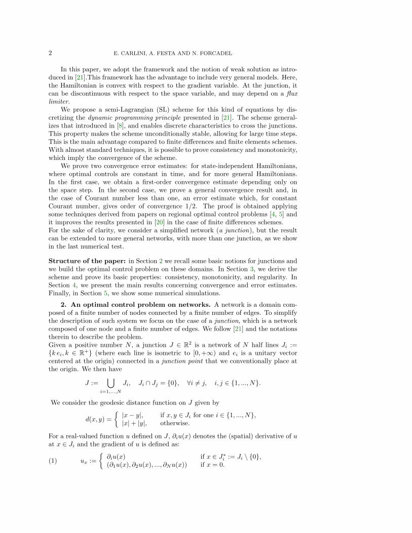
2. An optimal control problem on networks. A network is a domain com-posed of a finite number of nodes connected by a finite number of edges. To simplifythe description of such system we focus on the case of a junction, which is a networkcomposed of one node and a finite number of edges. We follow [21] and the notationstherein to describe the problem.Given a positive number N , a junction J ∈ R2 is a network of N half lines Ji :={k ei, k ∈ R+} (where each line is isometric to [0,+∞) and ei is a unitary vectorcentered at the origin) connected in a junction point that we conventionally place atthe origin. We then have

J :=⋃

i=1,...,N

Ji, Ji ∩ Jj = {0}, ∀i 6= j, i, j ∈ {1, ..., N}.

We consider the geodesic distance function on J given by

d(x, y) =

{|x− y|, if x, y ∈ Ji for one i ∈ {1, ..., N},|x|+ |y|, otherwise.

For a real-valued function u defined on J , ∂iu(x) denotes the (spatial) derivative of uat x ∈ Ji and the gradient of u is defined as:

(1) ux :=

{∂iu(x) if x ∈ J∗i := Ji \ {0},(∂1u(x), ∂2u(x), ..., ∂Nu(x)) if x = 0.

A SEMI-LAGRANGIAN SCHEME FOR HJ EQUATIONS ON NETWORKS 3

J1 J2

J3

J4

J5

e1

e3

e2

e4

e50

Fig. 1. Junction with N = 5 edges.

We describe a finite-horizon optimal control problem on the network J . For a moreextensive description of the problem, see [21].Let us define the set of admissible dynamics on the network J connecting the point(s, y) to (t, x) as

(2) Γt,xs,y :=

(X(·), α(·)) ∈ Lip([s, t]; J)× L∞([s, t];RN+1)

X(τ) = U(X(τ), α(τ)), τ ∈ [s, t]X(s) = y, X(t) = x

,

where for any (t, x) ∈ [0, T ]× J and α = (α0, α1, ..., αN ) ∈ RN+1 ,

U(x, α) =

{αi if x ∈ J∗iα0 if x = 0.

}.

We define the cost function,

L(x, α) :=

{Li(x, αi) if x ∈ Ji,L0(α0) if x = 0,

where the functions Li : R+ × R→ R for i = 1, . . . , N satisfy:(A1) Li are strictly convex (w.r.t. the second argument) and uniformly Lipschitz

continuous,(A2) Li are strongly coercive w.r.t. the second argument uniformly in x

(Li(x, αi)/|αi| → +∞ for |αi| → +∞ uniformly in x ∈ R+),(A3) for all µ > 0 there exists Cµ > 0 such that

supx∈Ji

∣∣∣∣ infαi∈[−µ,µ]

Li(x, αi)

∣∣∣∣ ≤ Cµ.In addition, L0 : R→ R is defined as

L0(α0) :=

{L0 if α0 = 0,+∞ otherwise,

for a given L0 ∈ R. The value function of the optimal control problem is

(3) u(t, x) = infy∈J

inf(X(·),α(·))∈Γt,x0,y

{u0(y) +

∫ t

0

L(X(τ), α(τ))dτ

}.


Remark. We stress on the generality of the model in treating the junction: anoptimal trajectory chosen in (2) is evaluated by the functional (3) where the cost doesnot have any regularity passing through the junction. The trajectories have also thepossibility of waiting in the junction paying a specific constant cost L0 per time unity.

It has been proved in [21] that the following dynamic programming principle(DPP) holds.

Proposition 2.1 (Dynamic programming principle). For all x ∈ J , t ∈ (0, T ],s ∈ [0, t), the value function u defined in (3) satisfies

(4) u(t, x) = infy∈J

inf(X(·),α(·))∈Γt,xs,y

{u(s,X(s)) +

∫ t

s

L(X(τ), α(τ))dτ

}.

A direct approximation of the DPP (4) is the basis for the scheme which wedescribe in the next section.The following Theorem characterizes the value function (3) as the solution of a HJBequation (for the definition of viscosity solution and the proof, see Appendix A and[21]).

Theorem 2.2 (HJB equation satisfied by the value function u). Given a functionu0, globally Lipschitz continuous on J , the value function u defined in (3) is the uniqueviscosity solution of

(5)

{∂tu(t, x) +Hi(x, ux(t, x)) = 0 in (0, T )× J∗i ,∂tu(t, x) + FA(ux(t, x)) = 0 in (0, T )× {0},

with initial condition u(0, x) = u0(x) for x ∈ J, where

Hi(x, p) := supαi∈R

{αi p− Li(x, αi)} ,

with pi(x) chosen such that Hi is non-increasing in (−∞, pi(x)] and non-decreasingin [pi(x),∞). The operator FA : RN → R on the junction point is

(6) FA(p) := max

(A, max

i=1,...,NH−i (0, pi)

), with A = −L0,

where

H−i (x, p) :=

{Hi(x, p) for p ≤ pi(x)Hi(x, pi) for p > pi(x).

Remark. In the vehicular traffic flow models, the function H− can be related,with suitable transformations, to the demand and supply functions, introduced in [23].This relation has been observed in [22]. In this setting, the constant A is known asthe flux limiter at the junction. In fact, the lower the cost at the junction L0 is, thelonger the vehicles will stay at the junction and so the bigger is the flux limiter.

We now gives some useful results on the Hamiltonian H.

Proposition 2.3 (Properties on H). Under assumptions (A1)-(A3), the fol-lowing assertions hold true:

i) for every x ∈ R+ ∪ {+∞} and bounded p, αi ∈ arg supαi∈R{αip− Li(x, αi)}is bounded.


ii) the nonincreasing part of Hi(x, p) with respect of pi is given by

H−i (x, pi) = supαi≤0{αipi − Li(x, αi)}.

iii) (Regularity). For all M > 0 there exists a modulus of continuity ωM suchthat for all |p|, |q| ≤M and x ∈ Ji

|Hi(x, p)−Hi(x, q)| ≤ ωM (|p− q|);

in addition, Hi(·, p) is Lipschitz continuous w.r.t. the space variable.iv) (Uniform coercivity). Hi(x, p) → +∞ for |p| → +∞ uniformly for every

x ∈ Ji ∪ {+∞}, i = 1, ..., N ;v) (Convexity). p 7→ Hi(x, p) is convex for every x ∈ J .vi) (Uniform bound of the Hamiltonian for bounded gradient). For all M > 0,

there exists CM > 0 such that

supp∈[−M,M ], x∈J∗

|H(x, p)| ≤ CM ,

where J∗ := J \ {0}.Remark. The previous proposition implies in particular the well-posedness of (5)

(see [21])

Proof. From assumptions (A1)-(A2), αip − Li(x, αi) is a continuous function(negatively) coercive, therefore there exists a compact interval [−µ, µ], µ ∈ R, suchthat

supαi∈R

{αi p− Li(x, αi)} = supαi∈[−µ,µ]

{αi p− Li(x, αi)} .

Since p is bounded, i) holds. Assertion ii) follows from Lemma 6.2 in [21].From i), we have

Hi(x, p)−Hi(x, q) ≤ α|p− q|

where α is the minimizer in Hi(x, q). Exchanging the role of p, q, we get iii).Taking α = 1 in the Hamiltonian we have

Hi(x, p) ≥ p− Li(x, 1).

The same argument for α = −1 gives Hi(x, p) → +∞ for |p| → +∞, then iv) holds.Finally v) holds since Hi is the upper envelope of convex functions and vi) followsdirectly from assumption (A3).

We now give regularity results for the value functions.

Proposition 2.4 (Regularity of the value function). Under assumptions (A1)-(A2), the value function u defined in (3) is Lipschitz continuous in space and time.

Proof. First, we remark that for C ≥ C0, with C0 defined as in vi) of Prop. 2.3with L = 0 , u0(x)± Ct are respectively subsolution and supersolution of (5). Usingthe comparison principle, we deduce that

u0(x)− Ct ≤ u(t, x) ≤ u0(x) + Ct.

Let h ≥ 0 and define uh(t, x) = u(t + h, x) − Ch. The previous inequalities impliesthat

uh(0, x) = u(h, x)− Ch ≤ u(0, x).


The equation is invariant by translation in time and by addition of constant (whichimplies that uh is a subsolution of (5)), then we get by the comparison principle that

uh(t, x) ≤ u(t, x).

This implies thatu(t+ h, x)− u(t, x)

h≤ C.

The reverse inequality can be proved in the same way (using that u(t+ h, x) +Ch isa supersolution), so we deduce that

|ut| ≤ C,

since h can be chosen arbitrary small. Hence u is Lipschitz continuous in time. Weknow that u is a viscosity solution of (5), therefore it satisfies in particular (in theviscosity sense) for each i ∈ {1, . . . , N}:

Hi(x, ux) ≤ C on (0, T )× J∗i .

Using the coercivity of H, this implies the existence of a constant C such that (in theviscosity sense)

|ux| ≤ C on (0, T )× J∗i .Therefore, u is Lipschitz continuous also with respect to the space variable.

Remark. Note that in the classical setting (i.e., without junction), this type ofresults can be obtained more directly using the definition of the value function andthe dynamic programming principle (obtaining first the regularity in space and thenin time). But the arguments use in this setting rely on the Lipschitz continuity of thecoset L which is no longer true at the junction. This is the reason why, in this proof,we have to used viscosity techniques.

3. A semi-Lagrangian scheme for the approximation of the solution.Let us introduce a uniform discretization of the network (0, T ) × J . The choice ofa uniform discretization is not restrictive, and the scheme can be easily extended tonon-uniform grids. Given ∆t and ∆x in R+, we define ∆ = (∆x,∆t), NT = bT/∆tc(b·c is the integer part) and

G∆ := {tn : n = 0, . . . , NT } × J∆x

where J∆x :=⋃i=1,...,N J

∆xi , J∆x

i = {k∆x ei : k ∈ N}. We define tn = n∆t forn = 0, . . . , NT and we derive a discrete version of the dynamic programming principle(5) defined on the grid G∆. To do so, as usual in first-order SL schemes, we discretize

the trajectories in Γtn+1,xtn,y by one step of Euler scheme. For i ∈ {1, . . . , N}, let x ∈ Ji

and let α ∈ RN+1 be such that αi∆t ≤ |x|, then the approximated trajectory gets

x ' y + αi∆t.

In this case, the discrete backward trajectory x −∆tαi remains on Ji and, applyinga quadrature formula, a discrete version of (4) at the point (tn+1, x) is

u(tn+1, x) ' u(tn, x− αi∆tei) + ∆tLi(x, αi).

Instead, if αi∆t > |x|, the discrete trajectory reaches the junction at a time in-

cluded in the interval [0,∆t]. Denoting by s0 ∈ [0,∆t − |x|αi ] the time spent by the


trajectory at the junction point, Jj the arc from which the trajectory comes, and

t :=(

∆t− s0 − |x|αi)

the remaining time on a new arc Jj , the approximation of (4)

at the point (tn+1, x) becomes

u(tn+1, x) ' u(tn,−αj tej

)+ t Lj(0, αj) + s0L0(α0) +

|x|αiLi(x, αi).

We denote B(J∆x) and B(G∆) the spaces of bounded functions defined respectivelyon J∆x and on G∆. We approximate the value function on the feet of the dis-crete trajectories, which in general are not grid nodes, by a standard piecewise linearLagrange interpolation I[u](z), where u ∈ B(J∆x) and z ∈ Jj , i.e.

I[u](z) := u(i∆xej) + (z − i∆xej)u((i+ 1)∆xej)− u(i∆xej)

∆xej,

for z ∈ [i∆xej , (i+ 1)∆xej).Finally, we define a fully discrete numerical operator S : B(G∆)× J∆x → R as, if

x ∈ Ji

S[v](x) := min

minαi<

|x|∆t

I[v](x− αi∆tei) + ∆tLi(x, αi),

minαi≥ |x|∆t

mins0∈[0,∆t− |x|αi ]

minj,αj≤0

{I[v]

(−(

∆t− s0 − |x|αi)αjej

)+(

∆t− s0 − |x|αi)Lj(0, αj) + s0L0(α0) + |x|

αiLi(x, αi)

},

and, if x = 0,

S[v](x) := minj,αj≤0

mins0∈[0,∆t]

{I[v] (− (∆t− s0)αjej)

+ (∆t− s0)Lj(0, αj) + s0L0(α0)} .

Then, the discrete solution w ∈ B(G∆) solves

(7) w(tn+1, x) = S[wn](x), n = 0, . . . , NT − 1, x ∈ J∆x

where wn := {w(tn, x)}x∈J∆x for n = 0, . . . , NT − 1 and w0 = {u0(x)}x∈J∆x .

3.1. Basic properties of the scheme. We prove some basic properties of (7):

Proposition 3.1 (Monotonicity and stability of the scheme). We assume that(A1)-(A3) hold. Then, the numerical scheme (7) is

i) monotone, i.e. given two discrete functions v1, v2 ∈ B(J∆x) such that v1 ≤ v2

we haveS[v1](x) ≤ S[v2](x), ∀x ∈ J∆x.

ii) invariant by addition of constants, i.e. S[ϕ + C](z) = S[ϕ](z) + C for anyconstant C.

iii) stable i.e. there exists a positive constant K such that for any (tn, x) ∈ G∆

|w(tn, x)− u0(x)| ≤ Ktn.

Proof. To prove monotonicity, let us fix a x ∈ J∆xi . We focus on the difficulty due

to the junction. More precisely, we assume that the trajectory related to v1 passes


through the junction and the one related to v2 does not. The other cases are easierand they can be treated in a similar way. Let us denote (αi, s0, j, αj , α0) the optimalstrategy contained in v1, and let us denote αi the optimal control of v2. The optimalcontrols are bounded by Prop. 2.3. We have

S[v1](x) = I[v1]

(−(

∆t− s0 −|x|αi

)αjej

)+

(∆t− s0 −

|x|αi

)Lj(0, αj)

+ s0L0(α0) +|x|αiLi(x, αi) ≤ I[v1](x− αi∆tei) + ∆tLi(x, αi) = S[v2](x),

which proves the monotonicity.The point ii) is a straightforward verification. The stability property iii) follows

directly by i) and ii) with K ≥ supx∈J∆x|S[u0](x)−u0(x)|

∆t . For the proof see [12] .

We now give a regularity result for the solution of the scheme. This is the discreteanalogue of the Lipschitz estimate in space of the value function. This will be usedin the proof of the error estimate.

Proposition 3.2. (Almost Lipschitz Regularity in space of w) Let w(tn, x) be asolution of (7). If u0 is uniformly Lipschitz continuous then for x, y ∈ J∆x thereexists a C > 0 such that

|w(tn, x)− w(tn, y)| ≤ C (∆t+ d(x, y)), n = 0, . . . , Nt.

The proof is postponed to Appendix B.

Remark. (Bounded control) By Prop. 3.1 iii), w solution of (7) is bounded andthen the discrete problem (7) is well-posed. We observe also that the same argumentof Proposition 2.3 (based on (A2)) can be used to prove that the control α in (7) isbounded. We define

(8) µ = sup(x,t)∈J×(0,T ]

maxi=1,...,N

|α∗i |,

the maximal absolute value of the optimal control.

3.2. Consistency of the scheme. We now focus on the study of the consistencyproperties of the scheme. First of all, we recall the definition of consistency, (the classof test functions C2(J) is defined in Appendix A).

Definition 3.3 (Consistency). Let x ∈ J and (∆xm,∆tm)→ 0 as m→∞. Letym ∈ J∆xm be a sequence of grid points such that ym → x as m→∞. The scheme Sis said to be consistent with (5) if the following properties hold:

i) If x ∈ Ji, for all test function ϕ ∈ C2(J), we have

(9)ϕ(ym)− S[ϕ](ym)

∆tm→ Hi(x, ϕx(x)) as m→∞,

ii) If x = 0, for all test function ϕ ∈ C2(J) such that ∂iϕ(0) = pL0i for i =

1, . . . , N , where pL0i ∈ R are such that Hi(0, p

L0i ) = H+

i (0, pL0i ) = −L0 and

H+i (x, p) := supαi≥0(αip− Li(x, α)), we have

(10)ϕ(ym)− S[ϕ](ym)

∆tm→ F−L0

(ϕx(x)) = −L0 as m→∞.


Definition 3.4 (Consistency estimate). Let x ∈ J∆x and ∆x,∆t > 0. We saythat the scheme S satisfies a consistency estimate E(∆x,∆t) > 0 if for all testfunction ϕ ∈ C2(J) with bounded second order derivatives, the following holds

i) If x ∈ J∆xi \ {0}, we have

(11)

∣∣∣∣ϕ(x)− S[ϕ](x)

∆t−Hi(x, ϕx(x))

∣∣∣∣ ≤ ‖ϕxx‖∞ E(∆x,∆t);

ii) If x = 0, we have

(12)

∣∣∣∣ϕ(x)− S[ϕ](x)

∆t− F−L0

(ϕx(x))

∣∣∣∣ ≤ ‖ϕxx‖∞ E(∆x,∆t);

Remark. Let us remark that, due to the particular form of the test function in(10), if the scheme admits a consistency estimates E(∆x,∆t) → 0, then the schemeis consistent in the sense of Definition 3.3. Indeed, if ym → 0 as m → +∞, withym ∈ J∗i and ϕ ∈ C2(J) with ∂iϕ(0) = pL0

i , then the consistency estimate implies

ϕ(ym)− S[ϕ](ym)

∆tm→ Hi(0, ϕx(0)) = Hi(0, p

L0i ) = −L0

We begin to prove some consistency estimates for the numerical operators.

Proposition 3.5. Given ∆t > 0 and ∆x > 0, let us assume the CFL condition

(13) µ∆t

∆x≤ 1, (with µ as in (8)),

then for any ϕ ∈ C2(J) the following estimates hold for (7):

i) if x ∈ J∆xi \ {0},

∣∣∣∣ϕ(x)− S[ϕ](x)

∆t−Hi(x, ϕx(x))

∣∣∣∣≤ K‖ϕxx‖∞

(∆t+ min(∆x,

∆x2

∆t)

),

ii) if x = 0,

∣∣∣∣ϕ(x)− S[ϕ](x)

∆t− F−L0

(ϕx(x))

∣∣∣∣≤ K‖ϕxx‖∞

(∆t+ min(∆x,

∆x2

∆t)

),

where K is a positive constant.

Remark. (Small Courant number) In the case very small Courant number areconsidered, µ∆t

∆x ≤ ∆x, the estimates in Prop. 3.5 ensure consistency error of order

1. These estimates improve the classical estimate ∆x2

∆t + ∆t for first order semi-Lagrangian scheme, and have first been proved in [14].

Proof. i) Let x ∈ J∆xi \ {0}. We remark that the condition (13) implies in

particular that the scheme reads

S[ϕ](x) = minαi<

|x|∆t

I[ϕ](x−∆tαiei) + ∆tLi(x, αi) = minαi∈R

I[ϕ](x−∆tαiei) + ∆tLi(x, αi).

By using recent estimates proved in [14, 15], we have

(14) I[ϕ](x−∆tαiei) = ϕ(x−∆tαiei) +K‖ϕxx‖∞ min(∆x2,∆t∆x),


then by standard Taylor expansion we get the result.ii) Let x = 0. In this case

S[ϕ](0) = mins0∈[0,∆t]

minj,αj≤0

{I[ϕ](−(∆t− s0)αjej) + (∆t− s0)Lj(0, αj) + s0L0(α0)} .

Let us define K∆t := s0∆t , since s0 ∈ [0,∆t] we have K∆t ∈ [0, 1]. Again by Taylor

expansion, by Prop. 2.3 and by the interpolation error (14), we have

maxϕ(0)− S[ϕ](0)

∆t+K‖ϕxx‖∞

(∆t+ min(∆x,

∆x2

∆t)

)= − min

K∆t∈[0,1]minj,αj≤0

(−(1−K∆t)αj∂jϕ(0) + (1−K∆t)Lj(0, αj) +K∆tL0(α0))

= − minK∆t∈[0,1]

[(1−K∆t) min

j,αj≤0(−αj∂jϕ(0) + Lj(0, αj)) +K∆t min

α0

(L0(α0))

]= maxK∆t∈[0,1]

[(1−K∆t) max

j,αj≤0(αj∂jϕ(0)− Lj(0, αj)) +K∆t max

α0

(−L0(α0))

]= maxK∆t∈[0,1]

{(1−K∆t) max

jH−j (0, ∂jϕ(0))−K∆tL0

}= max

(maxjH−j (0, ∂jϕ(0)),−L0

).

This ends the proof of the proposition.

The case that we study behaves differently from classic SL schemes, where theconsistency error estimate is not limited by a CFL condition. This difference is dueto the presence of discontinuities on the Hamiltonians at the junction point.

It is worth to underline that consistency (in the sense of Definition 3.3) holds evenwithout (13), and consequently the scheme is convergent without any CFL condition,as we show at the beginning of Section 4.

Proposition 3.6 (Consistency of the scheme). Assume min(∆x2

∆t ,∆x) → 0.Then, the scheme (7) is consistent according to Definition 3.3.

Proof. Let us consider a sequence ym such that ym → x as ∆m = (∆xm,∆tm)→(0, 0). For notational convenience we drop the index m of the sequence of grid points.In case the limit point x is not on the junction since x is fixed for every sequence(∆x,∆t)→ (0, 0), y eventually verifies |y| > µ∆t independently from the rate ∆t/∆x.Then, the consistency follows as Case 1 in the proof of Prop. 3.5 (without thecondition ∆t/∆x ≤ 1/µ).The situation is more complex when the limit point x is 0. If y ≡ 0, this case isequivalent to Case 2 in the proof of Prop. 3.5. If y is such that y → 0 and y 6= 0, upto a subsequence, we can assume that y ∈ Ji, for some i independent of m. In thatcase, the optimal trajectory can cross the junction in one time step. Let ϕ ∈ C2(J)such that ∂iϕ(0) = pAi for i = 1, . . . , N and let us define the two quantities:

I1 := minαi<

|y|∆t

(I[ϕ](y −∆tαiei) + ∆tLi(y, αi)),

I2 := minα,αi≥ |y|∆t

mins0∈[0,∆t− |y|αi ]

minj,αj≤0

{I[ϕ]

(−(

∆t− s0 −|y|αi

)αjej

)+

(∆t− s0 −

|y|αi

)Lj(0, αj) + s0L0(α0) +

|y|αiLi(y, αi)

}.


We remark that S[ϕ](y) = min(I1, I2). We begin with the term I1. Evaluating theinterpolation error and using a Taylor expansion, we get

I1 =

minαi≤ |y|∆t

{ϕ(y)− αi∆t∂iϕ(y) + ∆tLi(y, αi)}+K‖ϕxx‖∞(min(∆x2,∆t∆x) + ∆t2

)= ϕ(y)−∆t max

αi≤ |y|∆t

{αi∂iϕ(y)− Li(y, αi)}+K‖ϕxx‖∞(min(∆x2,∆t∆x) + ∆t2

)Using the inequality

maxαi≤ |y|∆t

{αi∂iϕ(y)− Li(y, αi)} ≤ maxαi∈R

{αi∂iϕ(y)− Li(y, αi)}

= Hi(y, ∂iϕ(y)) = −L0 + o(1),

we deduce that

(15) I1 ≥ ϕ(y)−∆tA+ ∆t o(1) +K‖ϕxx‖∞(min(∆x2,∆t∆x) + ∆t2

).

For the term I2, we add into the argument of ϕ the term y − |y|αi αiei = 0. Using theTaylor expansion twice and the interpolation accuracy, we obtain

I[ϕ]

(−(

∆t− s0 −|y|αi

)αjej

)= ϕ(y)− |y|

αiαi∂iϕ(y)−

(∆t− s0 −

|y|αi

)αj∂jϕ(0)

+K‖ϕxx‖∞(min(∆x2,∆t∆x) + ∆t2

).

The equation above implies

I2 +K‖ϕxx‖∞(min(∆x2,∆t∆x) + ∆t2

)= minαi≥ |y|∆t


{minj

minαj≤0

{−(

∆t− s0 −|y|αi

)(αj∂jϕ(0)− Lj(0, αj))

}+ ϕ(y)− |y|

αi(αi∂iϕ(y)− Li(y, αi)) + s0L0(α0)

}= ϕ(y) + min

αi≥ |y|∆t


{− |y|αi

(αi∂iϕ(y)− Li(y, αi)) + s0L0(α0)

−(

∆t− s0 −|y|αi

)maxj

maxαj≤0

{(αj∂jϕ(0)− Lj(0, αj))}}

= ϕ(y) + minαi≥ |y|∆t


{− |y|αi

(αi∂iϕ(y)− Li(y, αi)) + s0L0(α0)

−(

∆t− s0 −|y|αi

)maxjH−j (0, ∂jϕ(0))

}.

Using maxj H−j (0, ∂jϕ(0)) = maxj minpHj(0, p) =: H0, and L0(α0) = L0, we deduce


that (we use H0 ≤ −L0)

I2 +K‖ϕxx‖∞(min(∆x2,∆t∆x) + ∆t2

)= ϕ(y) + min

αi≥ |y|∆t

{− |y|αi

(αi∂iϕ(y)− Li(y, αi))

+ mins0∈[0,∆t− |y|αi ]

{s0(H0 + L0)−

(∆t− |y|

αi

)H0

}}= ϕ(y) + min

αi≥ |y|∆t

{− |y|αi

(αi∂iϕ(y)− Li(y, αi)) +

(∆t− |y|

αi

)L0

}(16)

= ∆t L0 + ϕ(y)− maxαi≥ |y|∆t

{|y|αi

(αi∂iϕ(y)− Li(y, αi) + L0)

}.

We use |y|αi ≤ ∆t in the last sup, and we observe that αi∂iϕ(y)−Li(y, αi) +L0 ≤ o(1)getting

(17) I2 +K‖ϕxx‖∞(min(∆x2,∆t∆x) + ∆t2

)≥ +∆t L0 + ϕ(y) + ∆to(1).

Finally, via (15) and (17), we obtain

(18) S[ϕ](y) = min(I1, I2)

≥ +∆tL0 + ϕ(y) + ∆to(1) +K‖ϕxx‖∞(min(∆x2,∆t∆x) + ∆t2

).

Now, we need to show that this inequality is in fact an equality. We denote by αi thesolution of

maxαi∈R{αi∂iϕ(y)− Li(y, αi)},

and distinguish two cases. Firstly, we consider the case αi ≤ |y|∆t . This implies in

particular that

maxαi≤ |y|∆t

{αi∂iϕ(y)− Li(y, αi)} = maxαi∈R{αi∂iϕ(y)− Li(y, αi)}

=Hi(y, ∂iϕ(y)) = −L0 + o(1).

Using (5), we deduce that

I1 = ∆tL0 + ϕ(y) + ∆to(1) +K‖ϕxx‖∞(min(∆x2,∆t∆x) + ∆t2

)and so (18) is an equality.

We now consider the case αi ≥ |y|∆t . We define

I2 := maxαi≥ |y|∆t

{|y|αi

(αi∂iϕ(y)− Li(y, αi) + L0)

}.

Clearly, 0 ≤ |y|αi ≤ ∆t and αi∂iϕ(y)− Li(y, αi) + L0 ≤ o(1), therefore we can say

∆t o(1) ≥ I2 ≥∆t

{maxαi≥ |y|∆t

{|y|αi

(αi∂iϕ(y)− Li(y, αi)}

+ L0

}=∆t(Hi(y, ∂iϕ(y)) + L0) = ∆t o(1).

This implies again that (18) is an equality and completes the proof.


4. Convergence and convergence estimates. In this section, we introducethe main results of the paper. First of all, the convergence of the scheme can beproven with a standard argument based on the monotonicity:

Theorem 4.1 (Convergence). Assume that min(∆x2/∆t,∆x)→ 0 and let T >0 and u0 be a Lipschitz continuous function on J . Then the numerical solution wof (7) converges uniformly on any compact set K of (0, T ) × J as ∆ → (0, 0) to theunique viscosity solution u of (5) , i.e.

lim sup∆x,∆t→0

sup(t,x)∈K∩G∆

|w(t, x)− u(t, x)| = 0.

Proof. Since the scheme is consistent (Prop. 3.6) for a subsequence verifyingmin(∆x2/∆t,∆x)→ 0, monotone and stable, we can follow [6, 11, 21] and obtain theresult. Note that the choice of the test functions in the definition of the consistencyat the junction uses Theorem A.2 ii)

Once shown the convergence of the scheme, we want to provide also some conver-gence estimates. This is a less easy task. We need to take into account two differentscenarios: for the special case of space independent Hamiltonians, i.e. assuming thefollowing additional property

(A4) the Lagrangians Li(x, αi) ≡ Li(y, αi) =: Li(αi) for every choice of x, y ∈ Ji,

it is possible to prove an error bound, independent of the time step. We observe that,as consequence of the structure of the costs, the optimal control αi is constant in timeand no restriction on the time step is required.

Theorem 4.2 (Rate of convergence in the case of space independent Hamiltoni-ans). Let (A1),(A2),(A4) be verified. Considered u a viscosity solution of (5), andw a solution of the scheme (7). Then, there exists a positive constant C dependingonly on the Lipschitz constant of u such that

(19) sup(t,x)∈G∆

|u(t, x)− w(t, x)| ≤ CT∆x.

The proof is contained in Appendix C.

For more general Hamiltonians (i.e. without assuming (A4)), we prove an errorbound that applies to any stable, monotone scheme for which a consistency estimateis valid.

Theorem 4.3 (Rate of convergence). Assume (A1)-(A3). Let u be the viscositysolution of (5), w be the solution of a scheme for which Prop. 3.1 holds and assumethat the scheme satisfies a consistency estimate E(∆t,∆x) as in Definition 3.4. Then,there exists a positive constant C independent of ∆t and ∆x such that

(20) sup(t,x)∈G∆

|u(t, x)−w(t, x)| ≤ CT(E(∆t,∆x)√

∆t+√

∆t

)+ supx∈J∆x

|u0(x)−w(0, x)|.

By applying the previous Theorem, we get an error estimate for scheme (7) undera restriction on the time step, given by assumption (13) .

Corollary 4.4 (Rate of convergence for (7)). In the specific case of the scheme(7), assuming (13), we have


(21) sup(t,x)∈G∆

|u(t, x)− w(t, x)| ≤ CT(√

∆t+1√∆t

min

(∆x2

∆t,∆x

)).

Remark. (CFL condition and error estimates) The CFL condition (13) is neededto prove the error estimate (21), and it is not assumed to prove the convergence resultin Theorem 4.1. If the assumption (A4) holds, no CFL condition is needed to provethe error estimate (19).

Proof. As standard in this kind of proof, we only prove that

(22) u(t, x)− w(t, x) ≤ C(E(∆t,∆x)√

∆t+√

∆t

)+ supx∈J∆x

|u0(x)− w(0, x)| in G∆,

since the reverse inequality is obtained with small modifications. Assume that T ≤ 1(the case T ≥ 1 is obtained by induction).

For i ∈ {1, . . . , N} and j ∈ N, we set xij = j∆xei, and we define the extension inthe continuous space of w as

w#(tn, x) = I[w(tn, ·)](x).

Firstly, we assume that

u0(xij) ≥ w#(0, xij) for all i ∈ {0, . . . , N} and j ∈ N,

and we define0 ≤ µ0 := sup

x∈J{|u0(x)− w#(0, x)|},

assuming without any restriction that µ0 ≤ K. For every β, η ∈ (0, 1) and σ > 0, wedefine an auxiliary function, for (t, s, x) ∈ [0, T )× {tn : n = 0, . . . , NT } × J

ψ(t, s, x) := u(t, x)− w#(s, x)− (t− s)2

2η− β|x|2 − σt,

Using Prop. 3.1 iii), the inequality |u(x, t) − u0(x)| ≤ CT (which holds for thecontinuous solution, see Theorem 2.14 in [21]), we deduce that ψ(t, s, x) → −∞ as|x| → +∞ and then the function ψ achieves its maximum at some point (tβ , sβ , xβ).In particular, we have

ψ(tβ , sβ , xβ) ≥ ψ(0, 0, 0) = u0(0)− w#(0, 0) ≥ 0.

In the following, we denote by K several positive constants only depending on theLipschitz constants of u.Case 1: xβ ∈ Ji \ {0}.In this case, we duplicate the space variable by considering, for ε ∈ (0, 1),

ψ1(t, s, x, y) =u(t, x)− w#(s, y)− (t− s)2

2η− d(x, y)2

2ε− β

2(|x|2 + |y|2)− σt

− β

2|x− xβ |2 −

β

2|y − xβ |2 −

β

2|t− tβ |2 −

β

2|s− sβ |2,

for (t, s, x, y) ∈ [0, T )× {tn : n = 0, . . . , NT } × J × J.


Using Proposition 3.1 iii) again, the inequality |u(x, t) − u0(x)| ≤ CT , and the factthat u0 is Lipschitz continuous, we deduce that ψ1(t, s, x, y)→ −∞ as |x|, |y| → +∞and then the function ψ1 achieves its maximum at some point (t, s, x, y), i.e.

ψ1(t, s, x, y) ≥ ψ1(t, s, x, y) for all (t, x), (s, y) ∈ [0, T )× J.

It is also easy to show that (t, s, x, y) → (tβ , sβ , xβ , xβ) as ε goes to zero and sox, y ∈ Ji \ {0}, for ε small enough.

Step 1. (Basic estimates). The maximum point of ψ1 satisfies the followingestimates:

(23) d(x, y) ≤ Kε, |t− s| ≤ Kη.

(24) β(|x|2 + |y|2

)≤ K, β

(|x− xβ |2 + |y − xβ |2 + |t− tβ |2 + |s− sβ |2

)≤ K

Fromψ1(t, s, x, y) ≥ ψ1(tβ , sβ , xβ , xβ)=ψ(tβ , sβ , xβ) ≥ 0,

we get, (using 0 ≥ −(t− s)2/2η − d(x, y)2/2ε− σt)

β

2(|x|2 + |y|2) +

β

2

(|x− xβ |2 + |y − xβ |2 + |t− tβ |2 + |s− sβ |2

)≤u(t, x)− w#(s, y) ≤ u0(x)− w#(0, y) +Kt+Ks ≤ K(1 + |x|+ |y|)(25)

where we used Proposition 3.1 i) (extended to all the points of J thanks to the mono-tonicity of the interpolation operator), [21, Theorem 2.14] for the second inequality,and the fact that T ≤ 1 for the last one. Using Young’s inequality, (i.e. the fact that|x| ≤ 1/β + β/4|x|2 since (β/2|x| − 1)2 ≥ 0) (25) implies in particular that

β

2(|x|2 + |y|2) ≤ K

(1 +

2

β+β

4(|x|2 + |y|2)

).

Multiplying by β and using β ≤ 1, we finally deduce that

β|x|, β|y| ≤ K.

Then using this in (25), we have

β(|x− xβ |2 + |y − xβ |2 + |t− tβ |2 + |s− sβ |2

)≤ K

(1 +

1

β

)and, in particular,

β (|x− xβ |+ |y − xβ |+ |t− tβ |+ |s− sβ |) ≤ K.

From ψ1(t, s, x, y) ≥ ψ1(t, s, y, y) we get

(26)d(x, y)2

2ε≤ u(t, x)− u(t, y) +

β

2(|y|2 − |x|2) +

β

2(|y − xβ |2 − |x− xβ |2)

≤ Kd(x, y) +β

2(|x|+ |y|)d(x, y) +

β

2(|x− xβ |+ |y − xβ |)d(x, y) ≤ Kd(x, y)


which implies the first estimate of (23). The second bound in (23) is deduced fromψ(t, s, x, y) ≥ ψ(s, s, x, y) in the same way.

If we include the estimate

u(t, x)− w#(s, y) ≤ u0(x) +Kt− w#(0, y)+Ks ≤ K(µ0 + d(x, y) + 1) ≤ K

in the first part of (25), we finally deduce (24).

Step 2. (Viscosity inequalities). We claim that for σ large enough, thesupremum of ψ1 is achieved for t = 0 or s = 0. We prove the assertion by contra-diction. Suppose t > 0 and s > 0. Using the fact that (t, x) → ψ1(t, s, x, y) has amaximum in (x, t) and that u is a subsolution, we get

(27)t− sη

+ σ + β(t− tβ) +Hi

(d(x, y)

ε+ β|x|+ β(|x− xβ |)

)≤ 0.

Since s > 0 we know that ψ1(t, s, x, y) ≥ ψ1(t, s − ∆t, x, y) for a generic y and, by

defining ϕ(s, y) = −(

(t−s)2

2η + d(x,y)2

2ε + β2 |y|

2 + β2 |y − xβ |

2 + β2 |s− sβ |

2)

, it implies

that, for a generic y,

w#(s, y)− ϕ(s, y) ≤ w#(s−∆t, y)− ϕ(s−∆t, y).

In particular, we have that for any z ∈ J∆x

w#(s, y)− ϕ(s, y) ≤ w(s−∆t, z)− ϕ(s−∆t, z).

By the monotonicity of the scheme and the fact that the scheme is invariant byaddition of constants, adding w#(s, y)− ϕ(s, y) we get, for any z ∈ J∆x,

w(s, z) = S[w(s−∆t)](z) ≥ S[ϕ(s−∆t)](z) + C.

By the monotonicity of the interpolation operator, this implies

w#(s, y) = I[w(s, ·)](y) ≥ I[S[ϕ(s−∆t)](·)](y) + w#(s, y)− ϕ(s, y).

Simplifying by w#(s, y), we obtain

−∑i

φi(y)S[ϕ(s−∆t)](yi) = −I[S[ϕ(s−∆t)](·)](y) ≥ −ϕ(s, y),

where φi are the basis functions of the interpolation operator. Adding and subtractingI[ϕ(s, ·)](y)− I[ϕ(s−∆t, ·)](y) and dividing by ∆t , we get

∑i

φi(y)

(ϕ(s−∆t, yi)− S[ϕ(s−∆t)](yi)

∆t+ϕ(s, yi)− ϕ(s−∆t, yi)

∆t

)≥ O

(∆x2

ε

),

where we have used ϕxx = O( 1ε ) together with the properties of the interpolation

operator. We observe that ϕ(s,yi)−ϕ(s−∆t,yi)∆t = ϕs(s, yi) + O(∆t/η), then, using the

consistency definition (Def 3.4), we obtain∑φi(y) (−ϕs(s, yi) +Hi(ϕx(s−∆t, yi))) ≥ O

(∆t

η+

∆x2

ε

)+E(∆t,∆x)

ε.


By the regularity of ϕ and H (Lipschitz continuous) and the interpolation error forLipschitz function, there exists a positive constant K such that

(28) ϕs(s, y) +Hi(ϕx(s−∆t, y)) ≥ −K(

∆t

η+

∆x2

ε

)+E(∆t,∆x)

ε.

We subtract (28) to (27) and use the explicit form of ϕ, obtaining

σ + β(s− sβ) + β(t− tβ) +Hi

(d(x, y)

ε+ β|x|+ β(|x− xβ |)

)−Hi

(d(x, y)

ε− β|y| − β(|y − xβ |)

)≤ K

(∆t

η+

∆x2

ε

)+E(∆t,∆x)

ε.

Then, using that Hi is Lipschitz continuous and the basic estimates of the Step 1, wearrive to

(29) σ < K√β +K

(∆t

η+

∆x2

ε

)+E(∆t,∆x)

ε=: σ∗.

Therefore, we have that for a σ ≥ σ∗ at least one between t and s is equal to zero.

Step 3. (Conclusion). If t = 0 (a similar argument applies if s = 0) we have

ψ1(0, s, x, y) ≤ u0(x)− w#(s, y) ≤ u0(x)− u0(y) + Cs+ µ0 ≤ Kε+Kη + µ0.

Taking σ = σ∗, we obtain

u(t, x)− w#(t, x)− β

2

(|x|2 + |y|2 + |x− xβ |2 + |y − xβ |2 + |t− tβ |2 + |s− sβ |2

)−(K√β +K

(∆t

η+

∆x2

ε

)+E(∆t,∆x)

ε

)T ≤ Kε+Kη + µ0.

Where, sending β → 0 and choosing ε = η =√

∆t, we get the desired estimate.

Case 2: xβ = 0.Firstly we observe that assuming

(30) σ > K√β +K

(E(∆t,∆x)

ε+

∆t

ε+

∆x

ε

)(which is compatible with σ > σ∗) then, there exists a A ∈ R such that

(31)sβ − tβη

−K(E(∆t,∆x)

ε+

∆t

ε

)+K

√β > A >

sβ − tβη

− σ +K√β.

Using the fact that (t, x) → ψ(t, sβ , x) has a maximum in (tβ , xβ) and that u is asubsolution, we get

(32)tβ − sβη

+ σ + F−L0(∂xϕ(tβ , 0)) ≤ 0,

with ϕ(t, x) = w#(sβ , x) +(t−sβ)2

2η + β|x|2 + σt and from (32) and (31),

(33) A > F−L0(∂xϕ(tβ , 0)) .


We use (33), the definition of F−L0, and the coercivity of the Hamiltonians to obtain

the existence of values λi such that

(34) Hi(λi) = H+i (λi) = A

(cf. Fig. 2) that will be useful in the remaining part of the proof.

H

H

H

1

2

3

p

A

λ3λ1λ2

Fig. 2. An example of H+i functions.

Now we pass to identify the right test function to treat this case. We duplicatethe space variable differently than in Case 1. We consider, for ε ∈ (0, 1),

ψ2(t, s, x, y) = u(t, x)− w#(s, y)− (t− s)2

2η− d(x, y)2

2ε− β

2(|x|2 + |y|2)

− σt− (h(x) + h(y))− β

2(t− tβ)2 − β

2(s− sβ)2,

for (t, s, x, y) ∈ [0, T )× {tn : n = 0, . . . , NT } × J × J.

where h(x) = λix if x ∈ Ji and the λi are defined in (34).We denote by (t, s, x, y) the maximum point of ψ2 (we keep the same notation

than the previous case, but they are possibly different points). We remark that(t, s, x, y)→ (tβ , sβ , xβ , xβ) as ε→ 0.

Step 2. (Viscosity inequalities). We claim that for σ large enough, thesupremum of ψ1 is achieved for t = 0 or s = 0. We prove the assertion by con-tradiction. Suppose t > 0 and s > 0. We can have different scenarios: if x and ybelong to the same arc (junction point excluded) the case is contained in Case 1. Ifinstead x ∈ Ji \{0}, y ∈ Jj (x and y belong to different arcs), we can repeat the sameargument to obtain (27) with the test function ψ2. We have:

t− sη

+ β(t− tβ) + σ +Hi

(d(x, y)

ε+ 2β|x|+ λi

)≤ 0.

Observing that the argument inside the Hamiltonian is bigger than λi, we use (34)arriving to

0 ≥ t− sη

+ β(t− tβ) + σ +H+i (λi) =

tβ − sβη

+ σ + A+K√β,


which contradicts (31). Then, this case cannot occur.We pass to the last case to consider: x = 0, y ∈ Ji \ {0}. First of all, we notice

that the basic estimates (23)-(24) are still valid for (t, s, x, y) maximum point of ψ2

since the added terms h(x), h(y) are easily included in the other linear elements ofthe estimates.

In this case, the difficulty comes comparing two Hamiltonians evaluated, respec-tively, on the junction point and on one arc. Using the subsolution property with thetest function ψ2, we have as first equation:

(35)t− sη

+ β(t− tβ) + σ + F−L0

(−|y|ε

+ λi

)≤ 0,

where

F−L0

(−|y|ε

+ λi

)= max

(−L0, max

j

(H−j

(−|y|ε

+ λi

))).

From the definition of FA it is also valid

(36)t− sη

+ β(t− tβ) + σ +H−i

(−|y|ε

+ λi

)≤ 0.

Since y ∈ Ji \ {0} with the same argument to obtain (28) (but for the test functionψ2) and using the consistency result, we have

t− sη

+ β(s− sβ) +Hi

(−|y|ε− 2βy + λi

)≥ K

(E(∆t,∆x)

ε+

∆t

η+

∆x2

ε

).

Now recalling that H+(λi) = A,

t− sη

+ β(s− sβ) +H+i

(−|y|ε− 2βy + λi

)−K

(E(∆t,∆x)

ε+

∆t

η+

∆x2

ε

)≤ t− s

η+ β(s− sβ) +H+

i (λi)−K(E(∆t,∆x)

ε+

∆t

η+

∆x2

ε

)≤ tβ − sβ

η+K

√β + A−K

(E(∆t,∆x)

ε+

∆t

η+

∆x2

ε

)< 0

for ε small enough, where we used β(s− sβ) ≤ K√β (basic estimates). We can claim

that

(37)t− sη

+ β(s− sβ) +H−i

(−|y|ε− 2βy + λi

)≥ K

(E(∆t,∆x)

ε+

∆t

η+

∆x2

ε

).

Finally, we subtract (37) to (35), obtaining the desired estimate on σ

(38) σ ≤ K√β +K

(E(∆t,∆x)

ε+

∆t

ε+

∆x

ε

):= σ∗.

In this case we obtain a contradiction with (30): since, assuming σ > σ∗, at least onebetween t and s is equal to zero.

Step 3. (Conclusion). We obtain the same estimate as in Case 1.

It just remains to prove the general case (for which we do not assume that u0(x) ≥w#(0, x),∀x ∈ J∆x). Remarking that u = u + µ1 with µ1 = supx∈J∆x(w#(0, x) −


-1 -0.8 -0.6 -0.4 -0.2 0 0.2 0.4 0.6 0.8 10

0.1

0.2

0.3

0.4

0.5

0.6

0.7

0.8

0.9

1 A=0

A=-0.2

A=-0.4

A=-0.6

u0

-1 -0.8 -0.6 -0.4 -0.2 0 0.2 0.4 0.6 0.8 10

0.2

0.4

0.6

0.8

1

1.2A=0

A=-0.2

A=-0.4

A=-0.6

Fig. 3. Initial condition and numerical solution at time t = 0.2 (left) and at time T = 2 (right),computed with parameter L0 = 0, 0.2, 0.4, 0.6.

u0(x)) is a solution of the same equation of u but satisfying u(0, x) ≥ w#(0, x),∀x ∈J∆x, we deduce that u satisfies

sup(t,x)∈G∆

(u(t, x) + µ1 − w(t, x))

≤ C(E(∆t,∆x)√

∆t+√

∆t

)+ supx∈J∆x

|u0(x) + µ1 − w(0, x)|.

which implies (22) ending the proof of the Theorem.

5. Numerical tests. In this section, we present some numerical simulations toshow the features and the convergence properties of the scheme proposed. In the firsttwo tests Assumptions (A1)-(A4) are verified, while in the last test (A4) does nothold.

Test 1. We consider a basic network composed by two edges connecting thenodes (−1, 0) and (1, 0) with a junction in 0. This case can be seen as an 1D problemin Γ = Γ1 ∪ Γ2 = [−1, 0] ∪ [0, 1] = [−1, 1] with a discontinuity on the Hamiltonian atthe origin. Despite its simplicity, this tests helps us to understand the effect of theflux limiter contained in the operator FA.We consider the following Hamiltonian on Γ:

H(x, p) =

{p2

2 −12 , x ∈ Γ1,

p2

2 − 1, x ∈ Γ2.

This example has been used as a benchmark also in [20]. Using the Legendre trans-form, we rewrite (5) as

H(x, p) =

maxα∈R

(α1p−

α21

2

)− 1

2, x ∈ Γ1,

maxα∈R

(α2p−

α22

2

)− 1, x ∈ Γ2.

where we can deduce L1(α1) = (α21 + 1)/2 and L2(α2) = (α2

1 + 2)/2. We chooseas initial condition u0(x) = sin(π|x|), and we impose Dirichlet boundary conditionsu(t,−1) = u(t, 1) = 0. The Dirichlet boundary condition are implemented numericallyby truncating the characteristics that cross the boundary, as in [15].


dx

0 0.02 0.04 0.06 0.08 0.1 0.120

0.1

0.2

0.3

0.4

0.5L0=0

E�

K dx

dx

0 0.05 0.1 0.150

0.1

0.2

0.3

0.4

0.5

0.6L0=0.2

E�

K dx

Fig. 4. Graphic of E∆∞ with respect the space step, together with the line K∆x. Left L0 = 0,

with K = 3.7, right L0 = 0.2, with K = 3.9.

In Fig.3, we show the numerical solution at time t = 0.2 and T = 2 computed withparameter L0 = 0, 0.2, 0.4, 0.6. We can observe as the asymmetry of the Hamiltonianwith respect to the origin induces an asymmetric behavior of the solution. We canalso highlight how the choice of parameter L0 influences globally the value functionof the problem. In fact, when L0 = 0 the optimal control in x = 0 is simply α0 = 0that corresponds to a zero cost, and since u0(0) = 0, the solution u(t, 0) = 0 for eacht ∈ [0, T ]. This explains the choice of the name flux limiter for L0: in this case theparameter blocks the passage of information between the two arcs which could besolved separately. In the case of L0 > 0 the situation is different: the control α0 = 0does not correspond to a null cost. A trajectory, which remains on the junctionpoint, entails a cost. Furthermore, we observe that for values of |L0| sufficientlylarge, the behavior of the solution does not change anymore with respect to L0. Thishappens because remaining on the junction point is no more a convenient choice,i.e., the transition condition (6) is reached only by one non-increasing Hamiltonian.Therefore, the flux limiter is not active anymore.In Figure 4, we show the convergence rates in the case of L0 = 0 and L0 = 0.2. Inabsence of an analytic exact solution, we compare the approximated solution w(T, x)with an approximation u(T, x) obtained on a very fine grid with ∆x = 10−4 and∆t = 2.5∆x. The error is evaluated with respect to the uniform discrete norm definedby

(39) E∆∞ := max

x∈J∆x(|w(T, x)− u(T, x)|).

The error E∆∞ as a function of ∆x is represented in Figure 4, for the choice L0 = 0

(left) and L0 = 0.2 (right), the final time T and the time step are fixed to T = 0.2and ∆t = 2.5∆x. We observe in the case L0 = 0 a linear decay of the E∆

∞ error,in particular, the E∆

∞ errors fit with a linear regression curve of ratio K1 = 3.7. Wealso observe the same convergence order in the case L0 = 0.2, with almost the sameratio K1 = 3.9. In this case, since Theorem 4.2 holds, their rate of convergence is 1independently of the choice of ∆t, so large time steps are allowed (cf. [15] where asimilar property is discussed for Euclidian domains).

Test 2. We consider a simple junction network composed by three edges connect-ing the nodes (0, 1), (−1,−1), (1,−1) with the junction point placed in (0, 0). Wedenote by J1 the edge connecting (0, 1) to (0, 0) and by J2, J3 the edges connecting(0, 0) to (1,−1) and (−1,−1), respectively. The cost function Li, i = 0, 1, 2, 3 are


-1 -0.5 0 0.5 1

-1

-0.5

0

0.5

1time=0

0

0.5

1

1.5

2

-1 -0.5 0 0.5 1

-1

-0.5

0

0.5

1time=0.5

0

0.5

1

1.5

2

-1 -0.5 0 0.5 1

-1

-0.5

0

0.5

1time=1

0

0.5

1

1.5

2

-1 -0.5 0 0.5 1

-1

-0.5

0

0.5

1time=1.5

0

0.5

1

1.5

2

Fig. 5. Projection on the state coordinate plane of the Initial Condition (top left), numericalsolution at time t = 0.5 (top right), t = 1 (bottom left) and t = 1.5 (bottom right).

defined as follows

Li(αi) =

α2i

2 + 1 if i = 1, 3,α2i

2 + 2 if i = 2,2 if i = 0, and α0 = 0,+∞ if i = 0, and α0 6= 0.

We impose Dirichlet boundary conditions on the boundary nodes:

u(t, x) =

{0 if x = {(−1,−1), (1,−1)},√

2 + 1 if x = {(0, 1)}.

The initial value u0 is chosen as the restriction of 1 + x2 on J , where we denote(x1, x2) = x. In Figure 5, we show the color map of the initial condition and of thenumerical solution at time t = 0.5, 1, 1.5, projected on the state coordinate plane. Itis possible to observe that the initial datum u0 (Fig. 5 left/top) quickly evolves tothe stationary solution (Fig. 5 right/bottom), which represents a weighted distancefrom the boundary points, with exit costs equal to the boundary values.

We compare the approximate solution at T = 1.5 with the exact solution of thecorresponding stationary problem; this makes sense since the approximate solutionhas already reached the steady state. The exact steady state solution is

(40) u(x) =

√

2 + x2, if x ∈ J1,

min(

2√

(x1 − 1)2 + (x2 + 1)2,√

2 + 2√x2

1 + x22

), if x ∈ J2,√

(x1 + 1)2 + (x2 + 1)2, if x ∈ J3.


0 0.01 0.02 0.03 0.04 0.05 0.06 0.07 0.080

0.01

0.02

0.03

0.04

0.05

0.06

dx

E�

K dx

Fig. 6. Graphic of E∆∞ with respect the space step, together with the line K∆x with K = 6.5.

In Figure 6, we show the behavior of the error (39) for various values of ∆x, setting∆t = 2.5∆x. We observe as in the first test a linear decay of the E∆

∞, allowing largetime steps.

Test 3. We conclude this section treating a more complex network. We considera network formed by 4-junctions and 8-arcs, defined in (x1, x2) ∈ R2 and connectingthe points V1 = (−2, 0), V2 = (−1, 0), V3 = (0, 2), V4 = (0, 1), V5 = (2, 0), V6 = (1, 0),V7 = (0,−2), V8 = (0,−1). We define the edges J1 = V1V2, J2 = V2V4, J3 = V2V8,J4 = V3V4, J5 = V4V6, J6 = V5V6, J7 = V6V8, J8 = V7V8. We choose the costs oneach arc as

Li(x, αi) =

{α2i

2 + (2 + x1)2, for i = 1, 2, 3, 4,α2i

2 + (−2 + x2)2 for i = 5, 6, 7, 8.

We set the costs on the junction points Vi with i = 2, 4, 8 (when the relative controlα0 is null) equal to L(Vi, α) = 4, and on V6 equal to L(V6, α) = 0.4. We impose zeroDirichlet boundary conditions on the boundary points Vi with i = 1, 3, 5, 7.We choose as discretization steps ∆x = 0.013, ∆t = 0.065 and as the initial conditionu0 = 2− (x2

1 +x22)/2. We observe that the CFL condition (13) is not verified, however

we have convergence since Th. 4.1 holds (but the estimate Th. 4.3 does not hold).In Figure 7, we show the initial value function and its evolution at different times. Weobserve that the value function starts from a symmetric configuration and it loosesits symmetry since the costs are not constant on the various edges of the network andthey also depend on x. We highlight also that an optimal trajectory does not stop onjunction points since it would run into a cost considerably higher than elsewhere inthe network. The only exception is in V6, where the waiting cost is 0.4, and it is wherethe value function assumes a local minimum. Clearly, for t → +∞ such minimumtends to disappear since the cost is positive. In Figure 8, we also compare the valuefunction at t = 1.4 with the value function computed with same data except than thecost in V6, which is set to L(V6, α) = 4. We observe that, since in this case the costto stop in V6 is higher, the local minimum disappears.

Choosing an effective Courant number is not a trivial task. In particular, largeCourant numbers can considerably increase the complexity of the scheme near thejunctions. In contrast, the opposite can produce low accuracy for long time approxi-mations due to numerical diffusion effects.In Table 1, we show the CPU times of a code implementing the proposed method for


Fig. 7. Evolution of the value function at times t = 0, 0.26, 0.52, 1.04.

Test 3. The code is written in MatLab R2018a and runs on a MacBookPro 2017 2.5GHz Intel Core i7. The variable nc represents the number of points used to computethe minimum by comparison, with respect to the time s0, in (3).The second and third columns show that the minimum complexity is reached when∆t = ∆x/8, which corresponds to the case when the discrete characteristics do notcross the junctions. Choosing a time step lower than ∆x/8 is no more convenientin terms of computational time. In the last column, we consider the case whenL(Vi, α) = 4 for i = 2, 4, 6, 8. This choice corresponds to the case in which the char-


Fig. 8. Comparison between the value functions varying the cost in V6, L(V6, α) = 0.4 (above)L(V6, α) = 4 (below) at time t = 1.04.

acteristics never stop on the junctions. Therefore the minimization with respect to s0

is not necessary, and nc is set to 1. In this case, the minimum complexity is reachedusing the largest time step.In conclusion, Table 1 shows that large time steps may imply higher complexity due tothe cost of exploring all the arcs and computing the minimum of the waiting time s0

on the junctions. However, in semi-Lagrangian schemes, large time steps correspondto less diffusive numerical approximations. Still, very large time steps can imply alow accuracy in the approximation of the characteristics (when the characteristics arenot straight lines). The best choice, in term of accuracy, may consist in choosing atime step which optimizes the consistency error proved in Prop. 3.5.

L(V6, α) = 0.4 L(V6, α) = 4∆t nc =3 nc =6 nc =14∆x 10.4 19.4 3.72∆x 9.8 19.0 3.7∆x 9.6 18.0 3.9∆x/2 8.8 15.6 4.1∆x/4 8.3 13.2 5.2∆x/8 7.4 7.5 7.2∆x/16 14.7 14.8 14.4∆x/32 29.5 30.0 28.5

Table 1CPU times in seconds for Test 3, computed with ∆x = 0.013

Appendix A. Definition of viscosity solution. Let us introduce the classof test functions. For T > 0, set JT = (0, T )×J . We define the class of test functions


on JT and on J as

Ck(JT ) = {ϕ ∈ C(JT ), ϕ ∈ Ck((0, T )× Ji, ∀i = 1, . . . , N)},

Ck(J) = {ϕ ∈ C(J), ϕ ∈ Ck(Ji), ∀i = 1, . . . , N}.

We recall also the definition of upper and lower semi-continuous envelopes u∗ and u∗of a (locally bounded) function u defined on [0, T )× J ,

u∗(t, x) = lim sup(s,y)→(t,x)

u(s, y) and u∗(t, x) = lim inf(s,y)→(t,x)

u(s, y).

We say that a test function ϕ touches a function u from below (respectively fromabove) at (t, x) if u− ϕ reaches a local minimum (respectively maximum) at (t, x).

Definition A.1 (Flux-limited solutions). Assume that the Hamiltonian satisfiessome standard hypotheses of regularity, convexity and coercivity and let u : [0, T )×J →R.

i) We say that u is a flux-limited subsolution (resp. flux-limited supersolution)of (5) in (0, T )×J if for all test function ϕ ∈ C1(JT ) touching u∗ from above(resp. u∗ from below) at (t0, x0) ∈ JT , we have

(41)ϕt(t0, x0) +Hi(x0, ϕx(t0, x0)) ≤ 0 (resp. ≥ 0) if x0 ∈ Ji,ϕt(t0, x0) + FA(ϕx(t0, x0)) ≤ 0 (resp. ≥ 0) if x0 = 0.

ii) We say that u is a flux-limited subsolution (resp. flux-limited supersolution)of (5) on [0, T )× J if additionally

(42) u∗(0, x) ≤ u0(x) (resp. u∗(0, x) ≥ u0(x)) for all x ∈ J.

iii) We say that u is a flux-limited solution if u is both a flux-limited subsolutionand a flux-limited supersolution.

In [21], an equivalent definition of viscosity solutions for (5) is proved. We usethis equivalent definition in particular in the definition of the consistency in Section3. In the following theorem, we adapt this result for Hamiltonians depending on x.The proof is a straightforward adaptation of the one in [21].

Theorem A.2 (Equivalent definition for sub/supersolutions).Let H0 = maxj minpHj(0, p) and consider A ∈ [H0,+∞). Given solutions pAi ∈ R of

(43) Hi

(0, pAi

)= H+

(0, pAi

)= A

let us fix any time independent test function φ0(x) satisfying, for i = 1, . . . , N ,

∂iφ0(0) = pAi .

Given a function u : (0, T )× J → R, the following properties hold true.i) If u is an upper semi-continuous subsolution of (5) with A = H0, for x 6= 0,

satisfying

u(t, 0) = lim sup(s,y)→(t,0), y∈J∗i

u(s, y),(44)

then u is a H0-flux limited subsolution.


ii) Given A > H0 and t0 ∈ (0, T ), if u is an upper semi-continuous subsolution of(5) for x 6= 0, satisfying (44), and if for any test function ϕ touching u from above at(t0, 0) with

ϕ(t, x) = ψ(t) + φ0(x),(45)

for some ψ ∈ C2 ((0,+∞)), we have

ϕt + FA (ϕx) ≤ 0 at (t0, 0),

then u is a A-flux limited subsolution at (t0, 0).iii) Given t0 ∈ (0, T ), if u is a lower semi-continuous supersolution of (5) for

x 6= 0 and if for any test function ϕ satisfying (45) touching u from above at (t0, 0)we have

ϕt + FA (ϕx) ≥ 0 at (t0, 0),

then u is a A-flux limited supersolution at (t0, 0).

Remark. In fact this theorem shows that, at the junction, it is sufficient to testwith test function having the form (45).

Appendix B. Proof of Prop. 3.2.

Proof. In this proof, we denote by C a constant that depends only on Li and thatmay change line to line and with Lf the Lipschitz constant of a generic function f .Let just assume that x, y ∈ Ji ∩ J∆x. The latter is not restrictive since if x ∈Jj ∩ J∆x, y ∈ Ji ∩ J∆x with j 6= i, we come back to the case of a comparison betweenpoint belonging to the same arc writing

|w(tn, x)− w(tn, y)| ≤ |w(tn, x)− w(tn, 0)|+ |w(tn, 0)− w(tn, y)| .

We denote αi the optimal control of S[wn−1](y) associated to the i-arc. We considerthree different cases:

1) αi < |y|/∆t with y 6= 0.In this case, we consider αi such that x−∆tαiei = y −∆tαiei. This means that

(46) |αi − αi| =|x− y|

∆t.

Using the suboptimal control αi for S[wn−1](x) yields

w(tn, x)− w(tn, y) ≤ I[wn−1] (− (x− αi∆tei)) + ∆tLi(x, αi)

− I[wn−1] (− (y − αi∆tei))−∆tLi(y, αi) ≤ ∆tLLi |αi − αi| ≤ LLi |x− y|.

2) 0 < |y|∆t ≤ αi. In this case the discrete trajectory starting from y passes through

the junction. We denote by (αi, s0, α0, j, αj) the optimal control associated withS[wn−1](y). We distinguish two subcases:

2.i) x = 0. In this case, we choose the suboptimal control (s0+ |y|αi , α0, j, αj) (if α0 6= 0,


we replace it by 0 in order to stay in the origin) obtaining

w(tn, x)− w(tn, y) ≤ I[wn−1]

(−(

∆t− s0 −|y|αi

)αjej

)+

(s0 +

|y|αi

)L0(α0)

+

(∆t− s0 −

|y|αi

)Lj(0, αj)− I[wn−1]

(−(

∆t− s0 −|y|αi

)αjej

)−(

∆t− s0 −|y|αi

)Lj(0, αj) − s0L0(α0)− |y|

αiLi(y, αi) ≤

|y|αi

(L0(α0)− Li(y, αi)) .

If αi ≥ 1, using that Li is Lipschitz continuous, we get that there exists a constant C(depending only on Li(y, 0) and the Lipschitz constant of Li) such that

|Li(y, αi)||αi|

≤ C.

Injecting the estimate above in (8) and using that L0(0) is bounded, we deduce

w(tn, x)− w(tn, y) ≤ C|y| = Cd(x, y).

If αi ≤ 1, since L0(0) and Li(αi) are bounded, there exists a constant C such that

w(tn, x)− w(tn, y) ≤ C |y|αi≤ C∆t.

We finally get that in all the cases, w(tn, x)− w(tn, y) ≤ C (∆t+ d(x, y)) .

2.ii) |x| > 0. In this case, we choose αi such that |x|αi = |y|αi

. This implies in particular

x− |x|αiαiei = y − |x|

αiαiei

and so |x|αi |αi − αi| = |x− y| = d(x, y). Using the suboptimal control (αi, s0, α0, j, αj)

for S[wn−1](x), we have

w(tn, x)− w(tn, y)

≤ I[wn−1]

(−(

∆t− s0 −|x|αi

)αjej

)+

(∆t− s0 −

|x|αi

)Lj(0, αj)

+ s0L0(α0) +|x|αiLi(x, αi)− I[wn−1]

(−(

∆t− s0 −|y|αi

)αjej

)−(

∆t− s0 −|y|αi

)Lj(0, αj)− s0L0(α0)− |y|

αiLi(y, αi)

≤ LLi|x|αi|αi − αi| ≤ LLid(x, y)

3) y = 0. We denote by (s0, α0, j, αj) the optimal control associated to the operatorS[wn−1](y). We distinguish two subcases again:

3.i) : s0 = ∆t. We choose αi ≥ max(1, |x|∆t ) and the suboptimal control (αi, s0− |x|αi , α0)


for S[wn−1](x) obtaining

w(tn, x)− w(tn, y)

≤ I[wn−1] (0) +

(s0 −

|x|αi

)L0(α0) +

|x|αiLi(x, αi)− I[wn−1] (0)− s0L0(α0)

≤ |x|αi

(Li(x, αi)− L0(α0)) ≤ LLid(x, y)

Using that Li is Lipschitz continuous, we get that there exists a constant C (dependingonly on Li(0), L0(0) and on the Lipschitz constant of Li) such that

|Li(x, αi)|+ |L0(α0)||αi|

≤ C.

This implies that w(tn+1, x)− w(tn+1, y) ≤ C|x| = Cd(x, y).

3.ii): s0 < ∆t. We choose αi ≥ max(1, |αj |) such that

(47)|x|αi≤ ∆t− s0

2and

∆t− s0

∆t− s0 − |x|αi|αj | ≤ αi.

We also set αj = ∆t−s0∆t−s0− |x|αi

αj , which satisfies in particular αi ≥ |αj |. Taking the

suboptimal control (αi, s0, α0, j, αj) for S[wn−1](x), we get

(48) w(tn, x)− w(tn, y) ≤ I[wn−1]

(−(

∆t− s0 −|x|αi

)αjej

)+

(∆t− s0 −

|x|αi

)Lj(0, αj) + s0L0(α0) +

|x|αiLi(x, αi)

− I[wn−1](− (∆t− s0) αjej

)− (∆t− s0)Lj(0, αj)− s0L0(α0)

≤ |x|αi

(Li(x, αi)− Lj(0, αj)

)+ (∆t− s0)

(Lj(0, αj)− Lj(0, αj)

)≤ |x|αi

(Li(x, αi)− Lj(0, αj)

)+ (∆t− s0)LLj |αj − αj |.

Using that αi ≥ 1, we get that |Li(x,αi)αi≤ C. In the same way (using that αi ≥ αj)

|Lj(0, αj)|αi

≤ 1

αi

(Lj(0, 0) + LLj |αj |

)≤ Lj(0, 0) + LLj

|αj |αi≤ C.

Finally, using the definition of αj , we observe that

(∆t− s0)|αj − αj | = |x||αj |αi≤ |x|.

Injecting these estimates in (48), we obtain w(tn, x)− w(tn, y) ≤ C|x| = Cd(x, y).

Appendix C. Proof of Theorem 4.2.

Proof. The proof is made by induction assuming that for n ≥ 1

(49) |wn−1(x)− u(tn−1, x)| ≤ (n− 1)C∆x ∀x ∈ J∆x.


Note that the thesis is clearly satisfied for n = 1. We then want to show that

|wn(x)− u(tn, x)| ≤ nC∆x ∀x ∈ J∆x.

From Proposition 2.1, we know that

(50) u(tn, x) := infy∈J

inf(X(.),α(.))∈Γtn,xtn−1,y

u(tn−1, y) +

tn∫tn−1

L(X(τ), α(τ))dτ

.,

where we use the notation L(X(τ), α(τ)) ≡ Li(αi) if X(τ) ∈ Ji, (see (A4)).We denote α = (α0, α1, ..., αN ) and s0 the optimal argument of S[wn−1](x) and

we treat only the case where x ∈ Ji\{0} and |x|/αi < ∆t (this corresponds to themore difficult case in which the optimal trajectory crosses the junction). We alsodenote by X(t) (with t ∈ [tn−1, tn]) the trajectory obtained applying the control α.

Clearly such trajectory belongs to Γtn,xtn−1,X(tn−1)

with X(tn−1) =(

∆t− s0 − |x|αi)ej

and

(51)

X(t) ∈ Ji for t ∈

[tn − |x|αi , tn

),

X(t) = 0 for t ∈[tn − |x|αi − s0, tn − |x|αi

),

X(t) ∈ Jj for t ∈[tn−1, tn − |x|αi − s0

].

Therefore,

u(tn, x)− wn(x) =

infy∈J

inf(X,α)∈Γtn,xtn−1,y

u(tn−1, y) +

tn∫tn−1

L(X(τ), α(τ))dτ

− S[wn](x)

≤u(tn−1, X(tn−1)) +

∫ tn

tn−1

L(X(τ), α(τ))dτ − S[wn](x)

≤u(tn−1, X(tn−1))− I[wn−1](X(tn−1))|

+

∫ ∆t− |x|αi −s0

0

L(X(τ), α(τ))dτ −(

∆t− s0 −|x|αi

)Lj(αj)

+

∆t− |x|αi∫∆t−s0− |x|αi

L(X(τ), α(τ))dτ − s0L0(α0) +

∆t∫∆t− |x|αi

L(X(τ), α(τ))dτ − |x|αiLi(αi).

Since L(., α) is constant in time, the cost terms cancel. Moreover, using standardinterpolation operator properties and (49), we observe that

u(tn−1, X(tn−1))− I[wn−1](X(tn−1))|=u(tn−1, X(tn−1))− I[u(tn−1, ·)](X(tn−1)) + (n− 1)C∆x

+ I[u(tn−1, ·)− (n− 1)C∆x](X(tn−1)) + I[wn−1](X(tn−1)) ≤ nC∆x,

and consequentlyu(tn, x)− wn(x) ≤ nC∆x.


For the inverse inequality, we invert the whole argument. An additional difficultycomes for the choice of the good control for the S[wn−1] term. We proceed consideringa continuous optimal control α(·) for u(tn, x) in (50). Without loss of generality weassume that the associated trajectory X(t) is such that

(52)

X(t) ∈ Ji, for t ∈ (t2, tn] ,X(t) = 0, for t ∈ (t1, t2] ,X(t) ∈ Jj , for t ∈ [tn−1, t1] ,

Indeed, we can exclude that an optimal trajectory passes in another arc or touchesmultiple times the junction point thanks to the convexity of the functions L. In fact,in such case, it would be necessary for an optimal trajectory to pass twice for thesame point, i.e. X(t1) = x and X(t2) = x, with X(t) 6= x for t ∈ (t1, t2). This meansthat since X(t) = α(t), we have that∫ t2

t1

α(τ)dτ = X(t1)−X(t2) = 0.

Then, the average control on [t1, t2] is zero. Using the strict convexity and the Jensen’sinequality, we find that the optimal control α should be zero. This contradicts thedefinition of X.

We can now build a discrete control and an associated trajectory (α, X) forS[ϕ](x) such that

αi =|x|

tn − t2=

1

tn − t2

∫ tn

t2

αi(τ)dτ, s0 = t2 − t1,

αj =1

t1 − tn−1

∫ t1

tn−1

αj(τ)dτ.

Then, by construction X(tn−1) = X(tn−1) and

S[wn−1](x)− u(tn, x) = S[wn−1](x)− u(tn−1, y) +

∫ tn

tn−1

L(X(τ), α(τ))dτ

≤I[wn−1](X(tn−1))− u(tn−1, X(tn−1)) + (∆t− t2)Li(αi)−∫ ∆t

t2

L(X(τ), α(τ))dτ

+

((t2 − t1)L0 −

∫ t2

t1

L(X(τ), α(τ))dτ

)+

(t1Lj(αj)−

∫ t1

tn−1

L(X(τ), α(τ))dτ

).

Using Jensen’s inequality knowing that the L-functions are convex, we get

t1Lj(αj)−∫ t1

tn−1

L(X(τ), α(τ))dτ

=t1Lj

(1

t1 − tn−1

∫ t1

tn−1

αj(τ)dτ

)−∫ t1

tn−1

Lj(αj(τ))dτ

≤∫ t1

tn−1

Lj(αj(τ))dτ −∫ t1

tn−1

Lj(αj(τ))dτ = 0


The two others cost terms can be treated in a similar way. Using that

I[wn−1](X(tn−1))− u(tn−1, X(tn−1)) ≤ I[wn−1](X(tn−1))

− I[u(tn−1, ·) + (n− 1)C∆x](X(tn−1)) + I[u(tn−1, ·)](X(tn−1))

+ (n− 1)C∆x− u(tn−1, X(tn−1)) ≤ nC∆x

for the basic properties of the interpolation operator and (49), we can claim that

wn(x)− u(tn, x) ≤ nC∆x

and this concludes the proof.

REFERENCES

[1] Y. Achdou, F. Camilli, A. Cutrı, and N. Tchou, Hamilton–jacobi equations constrained onnetworks, Nonlinear Differential Equations and Applications NoDEA, 20 (2013), pp. 413–445.

[2] B. Andreianov, K. H. Karlsen, and N. H. Risebro, A theory of l1-dissipative solvers forscalar conservation laws with discontinuous flux, Archive for rational mechanics and anal-ysis, 201 (2011), pp. 27–86.

[3] M. Bardi and I. C. Dolcetta, Optimal control and viscosity solutions of Hamilton-Jacobi-Bellman equations, Birkauser, 1996.

[4] G. Barles, A. Briani, and E. Chasseigne, A bellman approach for two-domains optimalcontrol problems in rn, ESAIM: Control, Optimisation and Calculus of Variations, 19(2013), pp. 710–739.

[5] G. Barles, A. Briani, E. Chasseigne, and C. Imbert, Flux-limited and classical viscos-ity solutions for regional control problems, ESAIM Control Optimisation and Calculus ofVariations, 24(4) (2018), pp. 1881–1906.

[6] G. Barles and P. E. Souganidis, Convergence of approximation schemes for fully nonlinearsecond order equations, Asymptotic Analysis, 4 (1991), pp. 271–283.

[7] F. Camilli, E. Carlini, and C. Marchi, A flame propagation model on a network withapplication to a blocking problem, Discrete Continuous Dynamical-Systems 11(5) (2018),pp. 825–843.

[8] F. Camilli, A. Festa, and D. Schieborn, An approximation scheme for a hamilton–jacobiequation defined on a network, Applied Numerical Mathematics, 73 (2013), pp. 33–47.

[9] F. Camilli, A. Festa, and S. Tozza, A discrete hughes’ model for pedestrian flow on graphs,Networks & Heterogeneous Media, 12 (2017), pp. 93–112.

[10] F. Camilli, C. Marchi, A comparison among various notions of viscosity solution for Hamil-ton–Jacobi equations on networks, Journal of Mathematical Analysis and Applications,407(1) (2013), pp. 112–118.

[11] G. Costeseque, J.-P. Lebacque, and R. Monneau, A convergent scheme for hamilton–jacobi equations on a junction: application to traffic, Numerische Mathematik, 129 (2015),pp. 405–447.

[12] M.G. Crandall, and P.-L. Lions, Two approximations of solutions of Hamilton-Jacobiequations, Math. Comp., 43 (1984),pp 1–19.

[13] E. Cristiani, B. Piccoli, and A. Tosin, Multiscale modeling of granular flows with applicationto crowd dynamics, Multiscale Modeling & Simulation, 9 (2011), pp. 155–182.

[14] F. Charles, B. Despres, and M. Mehrenberger, Enhanced convergence estimates for semi-Lagrangian schemes: application to the Vlasov-Poisson equation, SIAM Journal NumericalAnalysis, 51 (2013), pp. 840–863.

[15] M. Falcone and R. Ferretti, Semi-Lagrangian approximation schemes for linear andHamilton-Jacobi equations, vol. 133, SIAM, 2014.

[16] N. Forcadel and W. Salazar, Homogenization of second order discrete model and applicationto traffic flow, Differential and Integral Equations, 28 (2015), pp. 1039–1068.

[17] M. Garavello, K. Han, and B. Piccoli, Models for vehicular traffic on networks, vol. 9,American Institute of Mathematical Sciences (AIMS), Springfield, MO, 2016.

[18] M. Garavello, R. Natalini, B. Piccoli, and A. Terracina, Conservation laws with discon-tinuous flux, Networks & Heterogeneous Media, 2 (2007), pp. 159–179.

[19] M. Garavello and B. Piccoli, Traffic flow on networks, vol. 1, American institute of math-ematical sciences Springfield, 2006.


[20] J. Guerand and M. Koumaiha, Error estimates for finite difference schemes associated withhamilton-jacobi equations on a junction, Numerische Mathematik, 142(3) (2019), pp 525–575.

[21] C. Imbert and R. Monneau, Flux-limited solutions for quasi-convex hamilton-jacobi equations

on networks, Annales Scientifiques de l’ENS, (2017), pp. 357–448.[22] C. Imbert, R. Monneau, and H. Zidani, A hamilton-jacobi approach to junction problems

and application to traffic flows, ESAIM: Control, Optimisation and Calculus of Variations,19 (2013), pp. 129–166.

[23] J. P. Lebacque, The Godunov scheme and what it means for first order traffic flow models,In: Patriksson M., Labbe M. (eds) Transportation Planning. Applied Optimization, vol 64.Springer, Boston, MA, 2002.

[24] P.-L. Lions and P. Souganidis, Well-posedness for multi-dimensional junction problems withKirchoff-type conditions, Atti Accademia Nazionale Lincei Rendiconti Lincei MatematicaApplicata, 28 (2017), pp. 807–816.

[25] G. F. Newell, A simplified theory of kinematic waves in highway traffic, part i: Generaltheory, Transportation Research Part B: Methodological, 27 (1993), pp. 281–287.

[26] A. Quarteroni, R. Sacco, and F. Saleri, Numerical Mathematics, Texts in Applied Math-ematics 37, Springer-Verlag Berlin Heidelberg, 2007.

[27] D. Schieborn and F. Camilli, Viscosity solutions of eikonal equations on topological networks,Calculus of Variations and Partial Differential Equations, (2013), pp. 1–16.

[28] M. Treiber and A. Kesting, Traffic flow dynamics, Traffic Flow Dynamics: Data, Modelsand Simulation, Springer-Verlag Berlin Heidelberg, (2013).

a semi-lagrangian scheme for hamilton-jacobi …

Documents