a set of computer aided automatic control experiments for

A Set of Computer AidedAutomatic Control Experimentsfor Undergraduate StudentsYUSUF BUGDAY, MEHMET ONDER EFE

Department of Electrical and Electronics Engineering, TOBB University of Economics and Technology, Ankara, Turkey

Received 22 October 2009; accepted 24 May 2010

ABSTRACT: In a typical control systems course, students are expected to develop the notion of open loopand closed loop first. Under the feedback, traditional control theory offers many elegant solutions to controlproblems yet teaching those concepts experimentally is an art. This article describes how the notion of feedbackcontrol could be developed by utilizing a computer aided experimental setup available at the laboratories of TOBBUniversity of Economics and Technology. A DC motor control system is considered and step by step developmentof the understanding of feedback control is explained. Didactic aspect is taken care of throughout the manuscriptand extensions to research are emphasized. © 2010 Wiley Periodicals, Inc. Comput Appl Eng Educ 21: 300–312,2013; View this article online at wileyonlinelibrary.com/journal/cae; DOI 10.1002/cae.20472

Keywords: control experiments; undergraduate control education

INTRODUCTION

Use of computers and rapid increase in their speed and capabilitieswith affordable prices has been a strong influence on the engineer-ing education which have been blended with the computer-basedtools and approaches. Availability of several simulation softwareand development platforms have changed the teaching of engi-neering issues dramatically and today, the students, having allnecessary tools installed on their computers, have the capabilityof prototyping the ideas instantly. Furthermore, most institutionsare now covered by wireless networks enabling the students toaccess every kind of supplementary material. With such an amaz-ingly technology, computer, web, and communication centricenvironment, class materials as well as the teaching methods needcontinuous update. The field of automatic control is one of suchareas that influenced significantly from the possibilities offered bysuch advancements. Despite computer-based classroom teachingis one side of the whole issue; the other side is the exploitationof computer centric technologies in laboratory experiments thatencompasses the concepts of telelab, virtual lab, or web-basedinteractive lab. This article focuses on the laboratory side withthe goals of conveying a comprehensive understanding of feed-back, control, simulation, dynamics, frequency response, and keytechniques in the closed loop controller design such as PID, poleplacement, fuzzy control, and sliding mode control (SMC).

In the past, many works have been reported to describe thealternative methods utilizing computer aid in automatic control

Correspondence to M. O. Efe ([email protected]).© 2010 Wiley Periodicals, Inc.

experimentation. Duan et al. [1] consider a web enabled con-trol apparatus, an inverted pendulum, enabling the identification,prototyping, and refinement remotely. Another work reportinginternet-based experimentation is by Casini et al. [2], where itis emphasized that the proposed system does not require being inthe lab. The students perform the experiments remotely with hav-ing the full fledge of using Matlab/Simulink environment. Kamıset al. [3] present a motor control system developed for PID con-troller prototyping and typical transient responses and frequencyresponse pictures are given. Huba and Simunek focus on teach-ing PID control techniques via the WebLab described in Ref. [4],where the system level architecture and the security of the web sys-tem is highlighted together with the possibilities of implementingvarious models and controllers at different complexities. Anotherwork emphasizing the virtual instrumentation is due to Shahri [5],enabling web-based experimentation of Lead and Lag compen-sators. Wagner [6] stipulates 10 pragmatic design rules for thedevelopment of computer-assisted learning systems, and in Ref.[7] and overview of control education for several countries areelaborated.

Although web-based learning or remote learning is oneavenue, this article presents a computer-centric prototypingapproach requiring the student’s presence at the lab. Tested imple-mentations of the approaches adopted at the Department ofElectrical and Electronics Engineering of TOBB ETU are pre-sented. The article is organized as follows. The second sectiondescribes three simple experiments and simulations. The third sec-tion describes the DC motor control setup, and the experimentsdesigned on it are defined in the fourth section. The fifth sectionis devoted to the question of how this viewpoint can be connected

300

COMPUTER AIDED AUTOMATIC CONTROL EXPERIMENTS 301

to the viewpoint of a researcher. The structuring of the lab exper-iments and the concluding remarks are given at the end of thearticle.

SIMPLE EXPERIMENTS TO UNDERSTAND THENOTION OF FEEDBACK

This section describes several experiments where the computer useis restricted to simulation environments. The motivation of havingsuch a work in the lab work.

On–Off Control

Perhaps the simplest approach to describe feedback is based onon–off technique. In the laboratory, students are asked to build theresistor–capacitor system shown in Figure 1 and to figure out howon–off scheme could be implemented utilizing a single off-the-shelf operational amplifier (opamp). Most students remember thenonlinear saturating nature of opamp taught in the circuit analysiscourse and realize the feedback system should realize

u(t) ={

Vcc r(t) − y(t) > 0−Vcc r(t) − y(t) < 0

(1)

where Vcc is the supply voltage of the opamp and r(t) is the tar-get output. Once completed, the student comprehends the conceptof state, feedback, and on–off type control. The output of the firstorder system is forced toward a desired voltage and since all quan-tities are in voltages, it is easier for a student to attribute meaningto measured signals. This experiment is a quick start experimentavailable in the lab work of control systems course.

Figure 1 Pspice drawing of the system to be controlled. [Color figure canbe viewed in the online issue, which is available at wileyonlinelibrary.com.]

Control of a Second Order System: A SimulationExample

In this part, students are asked to determine the components ofa feedback control system depicted in Pspice environment. Thegiven design is shown in Figure 2 and the plant is composed of afirst order system followed by an integrator, which is described by(2).

y = −y + u (2)

Decomposing the blocks yields the dynamics above as wellas the controller that is composed of a proportional plus derivativeaction. The difference computer yields the error e = r − y, and thePD controller computes a control signal given by

u = e + 5e (3)

After understanding the role of each block, students realizethe same system in Matlab/Simulink environment and compare theresults for r(t) = 1 with zero initial conditions and t ≤ 5 s. The goal

Figure 2 Pspice drawing of the closed loop control system. [Color figure can be viewed in the online issue, which isavailable at wileyonlinelibrary.com.]

302 BUGDAY AND EFE

Figure 3 (a) Lowpass filter, (b) bandpass filter, and (c) highpass filter.[Color figure can be viewed in the online issue, which is available atwileyonlinelibrary.com.]

of such an experiment is to familiarize students with simulationtools like Matlab and Pspice, and to describe overshoot, rise time,peak time, and settling time concepts according to the obtainedresults.

Understanding the Frequency Domain

Teaching the frequency domain is one of the critical issues inalmost all engineering disciplines. The method we follow at thispart of the article is to describe three Sallen–Key filters designedfor lowpass, bandpass, and highpass behaviors. Students build thecircuits in Pspice environment, shown in Figure 3, and simulate for

Figure 4 (a) Analog control unit, (b) digital control unit, and (c) mechan-ical unit. [Color figure can be viewed in the online issue, which is availableat wileyonlinelibrary.com.]

sinusoidal inputs of unity magnitude with logarithmic frequencyvalues. The results are recorded, and then the approximate Bodemagnitude plots are constructed. The aim of such a simulationstudy is to gain an insight about justifying the theoretical resultsvia simulation.

DC MOTOR CONTROL SETUP

The motor control setup utilized in this work is composed of ahost computer, analog control unit shown in Figure 4a, the digital


Figure 5 PID controller to be realized. [Color figure can be viewed in the online issue, which is available atwileyonlinelibrary.com.]

control unit, shown in Figure 4b and a mechanical unit as shownin Figure 4c. An I/O card is installed into the host computer andthis card functions in providing the handshaking between thedigital control unit and the software platform, run by the hostcomputer. The analog unit provides experimenting proportional,integral, and derivative (PID) type controllers and variants, whilethe digital control unit enables implementing user-defined controllaws on Matlab/Simulink. The computer-assisted facility thereforeprovides a platform to develop novel control algorithms as well asthe conventional ones both for teaching and for research purposes.

Mechanical unit is equipped with a tachogenerator, analog,and digital encoders. The unit possesses a power amplifier todrive the installed DC motor and few standard reference signalsare generated on-board for possible trajectory tracking experi-ments. Practically, the introduced development platform is idealfor junior level students to develop a feeling of feedback con-trol, further, limited sampling rate and limited control voltagemakes it a good test bed for those pursuing research oriented solu-tions. The next section describes how such an experimental facilitycould be used in teaching the fundamental concepts of automaticcontrol.

LINEAR CONTROL EXPERIMENTS UTILIZING DCMOTOR CONTROL HARDWARE

This section describes the teaching approach based on the DCmotor control setup. The methodology contains analog and digitalcontrol examples demonstrating the concept progressively.

PID Control via Analog Control Unit

Due to their practical nature, well-explained dynamical responseand widespread preferability in industry, the most common tech-nique in the practice of automatic control systems is the PIDcontrollers and their variants. In the laboratory, we aim to demon-strate PID controller implementation on the DC motor controlsetup with analog unit shown in Figure 4a. The PID controllerstructure is shown in Figure 5, where it is possible to implementmany combinations of proportional, integral, and derivative effectsand to see their implications on the system response. Further, theavailable setup enables to reset the integrator manually. The phys-

ical connectivity is shown in Figure 6, which is simple enough torealize during a lab session.

After designing the controller and building the closed loopsystem on the analog unit, there are a number of steps that have tobe followed as a procedure by the students with manually apply-ing a step function as the input signal to the system. These stepsconsist of the trials of some variations for the coefficients of pro-portional, integral, and derivative actions. An exemplar input andoutput graph of the closed loop system is obtained on the oscillo-scope as given in Figure 7, where the PID coefficients are adjustedto the default settings provided by the manufacturer.

The students are asked to vary the coefficient of the propor-tional action for several times while keeping the coefficients ofintegral and derivative actions zero. They are directed to applystep function of magnitude 10 V for each parameter configurationand observe the motor position physically on the mechanical unitas well as on the oscilloscope. In the second step, integral andderivative actions are added to proportional control and the effectof integral action is investigated by varying the coefficient and bychanging the value of the capacitor in the feedback path of opera-tional amplifier, while the proportional and derivative coefficientsare constant. A similar process is repeated in the third step thatinvestigates the effect of derivative action while proportional andintegral coefficients are nonzero constants. Thus, the effects of theproportional, integral, and derivative actions on steady-state error,oscillations, rise time, and settling time of system response areseparately studied. In this manner, students gain an insight aboutone of the PID control scheme and practical considerations in itspractice.

Pole Placement Technique via Digital Control Unit

Pole placement method, a well-known approach of the controltheory, is based on the idea that the poles of a closed loop systemmay be placed at any desired location by means of state feed-back through an appropriate state feedback gain matrix under theassumption that the dynamic model of the system is known andcontrollability matrix has full rank. In this experiment the studentsare given the dynamic model of the system as given in (1) and (2).

The model of the DC servo motor system, located at themechanical unit mentioned before, is defined while neglecting thenonlinear characteristic added to system by the strap mechanism

304 BUGDAY AND EFE

Figure 6 Physical connectivity for the desired PID controller on analog unit.

between the wheels. State space model of single input single output(SISO) linear time invariant system can be considered as commonexpressions

x(t) = Ax(t) + Bu(t) (4)

y(t) = Cx(t) (5)

where x is state vector containing the angular position and angularvelocity, y is the output signal (angle), u is control signal (voltage)

and A =[

0 10 −4.76

], B =

[03.19

], C = [ 1 0 ] are constant

a-valued matrices, respectively. The control signal u(t) is defined

Figure 7 The response of the system to a step input.

as below

u(t) = −Kx(t) + pr(t) (6)

where r(t) represents the reference signal and K is the state feed-back gain matrix of dimensions 1 × 2 and p is a constant theis chosen to make steady-state error zero. Angular velocity isobtained from numerical derivative of the measured motor posi-tion. With this A and B, the system is full state controllable, thus thepoles of closed loop system can be mapped to any desired locationby choosing a proper gain matrix K. The task given to students isto map the closed loop system poles to s1 = 1.8, s2 = 1.9, whichwere chosen arbitrarily. Further, while choosing the pole values,physical limitations of the system have to be considered in order toobtain a physically realizable control signal and system response.Students are instructed to obtain the state feedback gain matrix Kin Matlab by utilizing “place” command which computes the gainmatrix by using the pair A, B, and the desired poles given above.Following this procedure, the students obtain the gain matrices fortwo different pairs of desired poles. After the calculation step ends,students realize the controller in Simulink environment, shown inFigure 8. The students are advised to smooth the angular speeddata as it is severely noisy. An exemplar realization is illustratedin Figure 8.

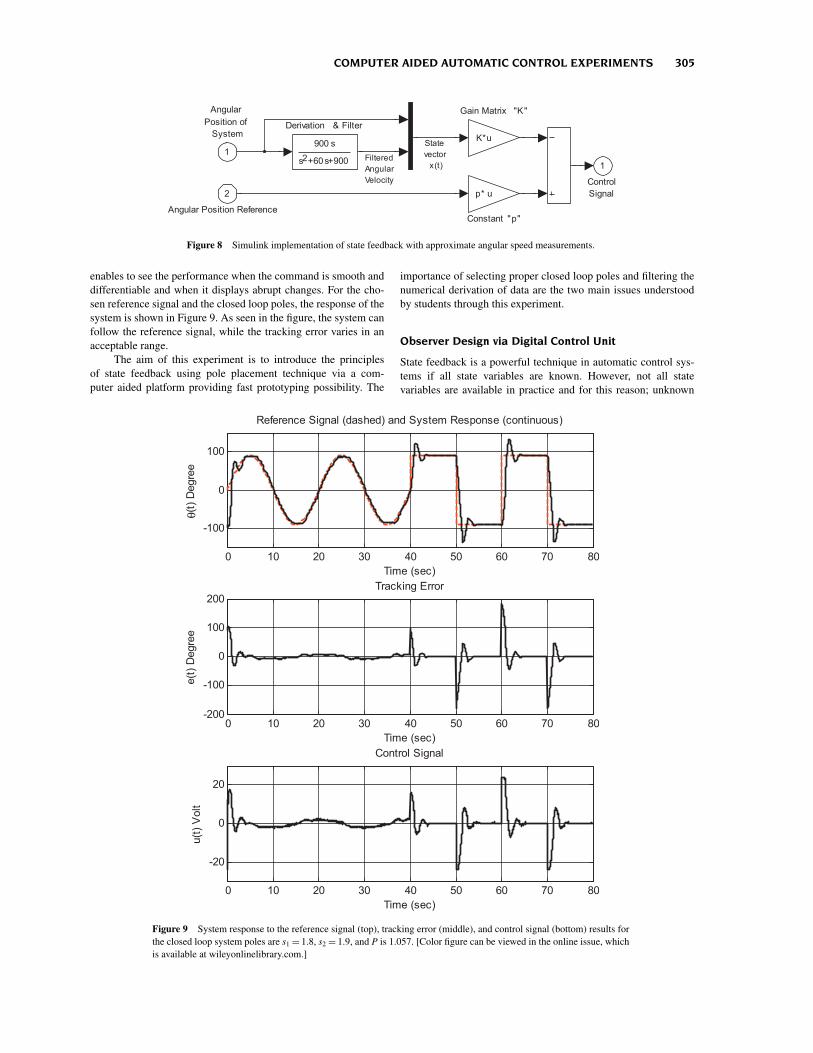
The angular position data of system, observed from themechanical unit via the digital control unit, and the control signal,driving the DC motor via digital control unit, are both availableas blocks in Simulink environment. A reference signal, which isa sine wave during the first 40 s and a square wave during thenext 40 s, is chosen. This particular choice of the reference signal


Control

Signal

1

Gain Matrix "K"

K*u

Derivation & Filter

900 s

s +60s+9002

Constant "p"

p* u

Angular Position Reference

2

Angular

Position of

System

1State

vector

x(t)Filtered

Angular

Velocity

Figure 8 Simulink implementation of state feedback with approximate angular speed measurements.

enables to see the performance when the command is smooth anddifferentiable and when it displays abrupt changes. For the cho-sen reference signal and the closed loop poles, the response of thesystem is shown in Figure 9. As seen in the figure, the system canfollow the reference signal, while the tracking error varies in anacceptable range.

The aim of this experiment is to introduce the principlesof state feedback using pole placement technique via a com-puter aided platform providing fast prototyping possibility. The

importance of selecting proper closed loop poles and filtering thenumerical derivation of data are the two main issues understoodby students through this experiment.

Observer Design via Digital Control Unit

State feedback is a powerful technique in automatic control sys-tems if all state variables are known. However, not all statevariables are available in practice and for this reason; unknown

0 10 20 30 40 50 60 70 80

-100

0

100

Reference Signal (dashed) and System Response (continuous)

Time (sec)

θ(t)

Degre

e

0 10 20 30 40 50 60 70 80-200

-100

0

100

200Tracking Error

Time (sec)

e(t

) D

egre

e

0 10 20 30 40 50 60 70 80

-20

0

20

Control Signal

Time (sec)

u(t

) V

olt

Figure 9 System response to the reference signal (top), tracking error (middle), and control signal (bottom) results forthe closed loop system poles are s1 = 1.8, s2 = 1.9, and P is 1.057. [Color figure can be viewed in the online issue, whichis available at wileyonlinelibrary.com.]

306 BUGDAY AND EFE

Estimated

State

1

Integrator

1

s

Ke* u

B* u

A* u

C* u

System

Output

2

Control

Signal

1

Figure 10 Simulink model of the observer designed in experiment.

state variables must be estimated by observers to be able to per-form the state feedback. In this sense, students are expected toobtain the state variables of the servo system by observers in thisexperiment. The mathematical model of the observer is defined asgiven in ()

˙x = Ax + Bu + Ke(y − Cx) (7)

where x is the estimated state and Ke is the observer gain matrixintensifying the error between the measured angular position ofthe system y and the estimated angular position Cx to improve thecorrectness of the estimation. The students are asked to calculatethe observer gain matrix Ke, given as

Ke = [ ke1 ke2 ]T (8)

Defining the error as e := x − x it is possible to derive thetracking error dynamics.

e = (A − KeC)e (9)

Claiming a desired pair of eigenvalues for the matrix A − KeCenables us to determine ke1 and ke2 . The observer is realized inMATLAB/Simulink environment as shown in Figure 10. The exter-nal control of the system is maintained by a PID controller whilethe observer predicts the system states.

By this way, students can easily apply various Ke gain matri-ces, calculated for different possible observer poles, to system andexperience the effects of the chose values of poles. Furthermore,estimated and measured states of the system are compared and per-formance of the observer is displayed in Figures 11 and 12 wherethe desired eigenvalues of A − KeC (the poles of the observer) ares1,2 = −1 for the first case and s1,2 = −8 for the second case. Itis seen from the figures that the students comprehend the varyingspeed of convergence for different Ke selections.

Through the experiment, extraction of the missing state vari-ables of a process is conveyed to the students. In this case, positionis measurable yet the angular speed is not. The observer providesa prediction for the angular speed. According to the results for thetwo selections, the students learn the observer is unable to catch ifits poles are not adequately away from the origin (see Fig. 11), if

0 10 20 30 40 50 60 70 80-500

0

500Measured state (dashed) and estimated state (continuous)

Time (sec)

Deg/s

ec

0 10 20 30 40 50 60 70 80-500

0

500Estimation Error

Time (sec)

Deg/s

ec

Figure 11 Motor speed estimation results for s1,2 = −1. [Color figure can be viewed in the online issue, which isavailable at wileyonlinelibrary.com.]


0 10 20 30 40 50 60 70 80-200

-100

0

100

200Measured state (dashed) and estimated state (continuous)

Time (sec)

Deg/s

ec

0 10 20 30 40 50 60 70 80-200

-100

0

100

200Estimation Error

Time (sec)

Deg/s

ec

Figure 12 Motor speed estimation results of for s1,2 = −8. [Color figure can be viewed in the online issue, which isavailable at wileyonlinelibrary.com.]

they are chosen appropriately, the observer removes the spuriouscontent in the angular speed and produces a much smoother speeddata as shown in the top row of Figure 12.

NONLINEAR CONTROL EXPERIMENTS

This section dwells on how the concepts of linear control canbe extended to nonlinear control laws while maintaining stabilityand performance expectations. Two popular approaches are exper-imented, namely, SMC and fuzzy control, which are explained inthe sequel.

Sliding Mode Control via Digital Control Unit

SMC is one of the most popular nonlinear control schemes usedfrequently in the literature. The philosophy of the design based onthe guidance of the error vector toward a predefined subspace of thephase space, called the sliding manifold, and to maintain it there.The design of this subspace, on the other hand, is a particularlyselected one, such that once the error vector gets trapped to it, themotion thereafter takes place in the vicinity of this subspace andthe error (and its derivatives) converge the origin [8–10].

Referring to the state space model described in (4) and (5), wedefine the errors as e1 = x1 − r1 is the positional error, e2 = x2 − r2,is the error in angular velocity with r2 = r1 and r2 is differentiabletoo. Define the switching variable as

�= e2+ � e1 =(

d

dt+ �

)e1 (10)

where the positive valued parameter � determines the slope ofthe line in the space spanned by e1 and e2. After taking the timederivative of (10) and exploiting (4) and (5) lets us have the control

input in the expression as given below

� = e2+ � e1

= x2 − r2+ � e2

= −4.76x2 + 3.19u − r2+ � e2

(11)

Clearly for a Q > 0, a reaching dynamics given by � =−Q sgn(�) would force any initial value of � to zero. Equating(11) to −Q sgn(�) and solving for the control signal lets us have

u = 1

3.19(4.76x2 + r2− � e2 − Q sgn(�)) (12)

The control law above ensures � = 0 in finite time, further,it introduces a certain level of robustness against modeling uncer-tainties such as the adverse effect of the belt used in this system. Inthe practice, the sign function is replaced by the function in (13)to avoid the chattering, a phenomenon that arises due to the signmeasurement of a quantity that is close to zero.

sgn(z) ∼= z

|z|+ �, �> 0 (13)

In this experiment, the effects of the following on the systemresponse are investigated.

• Reaching law parameter Q.• The slope parameter �.• The sign function smoothing parameter �.

The sliding mode controller in (12) is realized in the Simulinkenvironment with the aforementioned approximate angular veloc-ity information. Students are expected to vary the three parametersmentioned above, thus they analyze the characteristics and quali-ties of the system response as well as the control signal peculiar toeach specific case.

308 BUGDAY AND EFE

0 10 20 30 40 50 60 70 80-100

-50

0

50

100Reference Signal (dashed) and System Response (continuous)

Time (sec)

θ(t)

Degre

e

0 10 20 30 40 50 60 70 80-200

-100

0

100

200Tracking Error

Time (sec)

e(t

) D

egre

e

0 10 20 30 40 50 60 70 80

-20

0

20

Control Signal

Time (sec)

u(t

) V

olt

Figure 13 System response to the reference signal (top), tracking error (middle), and control signal generatedby the sliding mode control (bottom). [Color figure can be viewed in the online issue, which is available atwileyonlinelibrary.com.]

Initially, the values of �, �, and Q are selected as 2, 0.8, and10, respectively. Thus, the system response follows the desiredreference signal with an admissible level of error as seen in Figure13. When the reference signal suddenly changes, the controllerproduces a high amplitude signal locally in order to force the valueof � toward zero. For safety reasons, the control signal is withinthe range ±24 V and when there are abrupt changes, the controlsignal is likely to reach (or saturate at) these hard bounds.

The phase space behavior of error is illustrated as subplotsin Figure 14. The top left subplot depicts the reaching phase ofthe experiment, where we see that the error vector hits the slidingline and remains in the vicinity of it. In the top right subplot,the students see the sliding mode, which guide the error vectortoward the origin of the phase space. After the 40 s of run, squarewave reference signal becomes active, the controller is still able tostabilize the system yet it is difficult to see the sliding regime asclear as in the sinusoidal reference case.

Three parameters, namely �, �, and Q, characterizing theresponse of the controlled system, are varied on a one-at-a-timebasis. Increasing the value of reaching law parameter Q pro-vides faster reaching, more robustness but causes more chattering.

Increasing the value of slope parameter � provides faster con-vergence during the sliding mode. Increasing the value of signfunction smoothing parameter � worsens robustness; on the otherhand decreasing � magnifies the chattering. The students acquirehow a robust control law is implemented and the dependence ofperformance on the design parameters is understood.

Fuzzy Control via the Digital Control Unit

Fuzzy control is another nonlinear control experiment available inthe description of the laboratory. The philosophy that lies behindis based on the descriptions in terms of linguistic quantities. Theway to describe these quantities is to define membership functionscharacterizing sets whose boundaries are unsharp, that is, fuzzy,[X]. Fuzzy control is an active research field and the goal of theexperiment is to teach the basics of fuzzy control as well as estab-lishing links in between the undergraduate level control educationand its research extensions. The first step of the experiment is tounderstand the fuzzy quantification of a variable called e. In Figure15, three fuzzy sets are depicted which were asked once for everynew value of e, which changes in time.


-20 0 20

-20

0

20

e1(t) Degree

e2(t

) D

egre

e/s

ec

Phase Space for Sinusodial Reference

t=0-5 (sec)

-20 0 20

-20

0

20

e1(t) Degree

e2(t

) D

egre

e/s

ec

Phase Space for Sinusodial Reference

t=25-30 (sec)

-20 0 20

-20

0

20

e1(t) Degree

e2(t

) D

egre

e/s

ec

Phase Space for Square Reference

t=50-55 (sec)

-20 0 20

-20

0

20

e1(t) Degree

e2(t

) D

egre

e/s

ec

Phase Space for Square Reference

t=60-65 (sec)

Figure 14 The trajectories of the error in the phase space for different periods of an experiment. [Color figure can beviewed in the online issue, which is available at wileyonlinelibrary.com.]

If a different process is to be activated according to differentregional values of e, fuzzy logic is the best alternative to partitionthe input spaceR, to which e belongs, and activates dedicated pro-cesses whenever the necessary premises are held to a good extent.More explicitly, for two input and single output fuzzy system, therules of the form.

IFe1 ∈ Piande2 ∈ WiTHENu = yi

determine the local conclusion and the fuzzy system interpolates inbetween many such local conclusions to build a global map. In theabove rule structure, Pi and Wi denote the fuzzy sets correspondingto some linguistic label, positive, negative, or zero (see Fig. 15).

µN

µZ

µP

e

e

e

−L

−L L

L

1

1

1

Figure 15 Membership functions, negative (N) is on the top, zero (Z) isin the middle, and positive (P) is at the bottom.

In this experiment, a standard Sugeno type fuzzy controlleris used and defined by R = 9 rules with triangular membershipfunctions as shown above. Position error (e1) and its derivative(e2) are applied as inputs to fuzzy controller. Input and outputrelation is given as in (14).

u =

R∑i=1

yi

m∏j=1

�ij (ej)

R∑i=1

m∏j=1

�ij (ej)

(14)

Membership functions, seen in (14) and depicted in Figure15 are described explicitly as

�N (e) = max(

min(

− e

L, 1

), 0

)(15)

�Z (e) = max(

min(

1 + e

L, 1 − e

L

), 0

)(16)

�P (e) = max(

min(

e

L, 1

), 0

)(17)

The membership functions with a design parameter L areimplemented in Simulink environment and the overall fuzzy con-troller in (14) is then realized for experimentation. The teachinggoal here is to convey the effect of different L and yi (i = 1, 2, . . . ,R) selections on the performance. The latter describes the defuzzi-fier, which converts the fuzzy quantities to crisp values. Initiallythe students are given the value of L quantifying the positional erroras 33◦ and that quantifying the error in the angular speed as 82◦/s.Likewise, the an initial selection for the defuzzifier parameters (y)is as given below (Fig. 16)

y = [ −22 −16 −8 −2 0 2 8 16 22 ]T (18)

310 BUGDAY AND EFE

0 10 20 30 40 50 60 70 80-100

-50

0

50

100Reference Signal (dashed) and System Response (continuous)

Time (sec)

θ(t)

Degre

e

0 10 20 30 40 50 60 70 80-200

-100

0

100

200Tracking Error

Time (sec)

e(t

) D

egre

e

0 10 20 30 40 50 60 70 80

-20

0

20

Control Signal

Time (sec)

u(t

) V

olt

Figure 16 System response to the reference signal (top), tracking error (middle), and control signal generated by fuzzycontroller (bottom). [Color figure can be viewed in the online issue, which is available at wileyonlinelibrary.com.]

Defined control surface and obtained results are shown inFigure 17. The closed loop performance of the fuzzy controller issimilar to sliding mode controller, however, the transient responseof the system has shorter rising and settling times while usingfuzzy controller by choosing proper values for yi, providing fasterconverging. Besides, the steady-state performance of the fuzzycontroller is sufficiently good.

The aim of the experiment is to teach how feedback controlcan be accomplished without knowing the system dynamics. Sincethe student perform several experiments before trying the fuzzycontrol approach, they get a solid understanding of the DC motordynamics and they become capable of writing the rules to stabilizethe plant at a desired setpoint or around a desired trajectory asshown in Figure 14.

STRUCTURING THE LABORATORY EXPERIMENTS

Most engineering institutions offer the first control course in thethird year of the undergraduate education. This course typically

encompasses the topics from the ordinary linear differential equa-tions to preliminary concepts of state space analysis. The courses

-60-40

-200

2040

60

-100

0

100

-20

-10

0

10

20

e1(degree)e

2(degree/sec)

u(V

olt)

Figure 17 Control surface with the fuzzy system in (14). [Color figure canbe viewed in the online issue, which is available at wileyonlinelibrary.com.]


Table 1 Implementation Scheme for Junior and Senior Level Students

Experiment name 3rd class students 4th class students

On–off control Experiment #1 Prelab study #1Control of a second order system: A simulation example Experiment #2 Prelab study #2Understanding the frequency domain Experiment #3 Prelab study #3PID control via analog control unit Experiment #4 Experiment #1Pole placement technique via digital control unit Experiment #5 Experiment #2Observer design via digital control unit Experiment #6 (optional) Experiment #3Sliding mode control via digital control unit Not included Experiment #4Fuzzy control via digital control unit Not included Experiment #5

at the senior level are more diverse containing the state space anal-ysis, robust and nonlinear control techniques in depth. This articledescribes a set of laboratory experiments that is adaptable to both3rd and 4th year students as detailed in Table 1. The assessmentof the laboratory grade is based on the student’s performance dur-ing the experiment as well as the report submitted till the next labsession.

Regarding the learning of the course material, students’ fun-damental gain is to get a solid understanding of the concept offeedback. Further, during the course, the students perform sev-eral simulations, where components behave ideally, and they graspthe notion of imprecision during the real-time experiments. Thequality of the feedback signal directly influences the closed loopperformance and this is understood as a critical parameter influ-encing the performance of different control schemes. Anotherimportant gain of the students is to develop a an engineeringfeeling, that is, complicated control laws could yield better pre-cision yet simpler ones like the PID scheme are easy to implementwith cheap hardware. Last but not the least, after completing thedescribed set of experiments, the students have a clear under-standing of the frequency domain and the frequency response ofdynamic systems. Overall, the students experience the key notionsof the control systems through the described experiments.

CONCLUSIONS

This article describes several experiments that familiarize the con-trol engineering students with the use of simulation tools as wellas real-time design and implementation issues. The novelty intro-duced here is the method followed. To emphasize once more, theuse of simple strategies to convey the fundamental ideas of feed-back control is possible via simulation tools yet to understandbetter, several experiments are described to strengthen the feelingof feedback and closed loop control expectations. The consideredexperimental setup is a good test bed for junior level students tak-ing the automatic control course as well as for the students whoaim at solving research problems and prototype nonlinear controllaws on a physical system having limited computational capabili-ties. The article also provides how the experiments can be groupedto address 3rd and 4th class engineering students separately.

ACKNOWLEDGMENTS

This work was supported by TUBITAK contract no 107E137.

REFERENCES

[1] B. Duan, K.-V. Ling, H. Mir, M. Hosseini, and R. K. L. Gay, Anonline laboratory framework for control engineering courses, Int JEng Educ 21 (2005), 1068–1075.

[2] M. Casini, D. Prattichizzo, and A. Vicino, The automatic controltelelab: A user friendly interface for distance learning, IEEE TransEduc 46 (2003), 252–257.

[3] Z. Kamıs E. E. Topcu, and I. Yuksel, Computer aided automaticcontrol education with a real-time development system, Comput ApplEng Educ 13 (2005), 181–191.

[4] M. Huba and M. Simunek, Modular approach to teaching PID control,IEEE Trans Ind Electron 54 (2007), 3112–3121.

[5] A. M. Shahri, Advanced Control E-Laboratory (ACeL) Based onVirtual Instrumentation, IEEE CCECE 2003 Canadian Conferenceon Electrical and Computer Engineering, Montreal, Canada, Vol. 1,pp. 1–4, May 4–7, 2003.

[6] B. Wagner, From Computer Based Teaching to Virtual Laborato-ries in Automatic Control, 29th ASEE/IEEE Frontiers in EducationConference, San Juan, Puerto Rico, November 10–13, 1999.

[7] IEEE Control Systems Magazine, April 1996.[8] J. Y. Hung, W. Gao, and J. C. Hung, Variable structure control: A

survey, IEEE Trans Ind Electron 40 (1993), 2–22.[9] K. D. Young, V. I. Utkin, and U. Ozguner, A Control Engineer’s

Guide to sliding mode control, IEEE Trans Control Syst Technol 7(1999), 328–342.

[10] X. Yu and O. Kaynak, Sliding-mode control with soft computing: Asurvey, IEEE Trans Ind Electron 56 (2009), 3275–3285.

BIOGRAPHIES

Yusuf Bugday received the B.Sc. Degree fromthe Department of Electrical and ElectronicsEngineering, TOBB University of Economicsand Technology (Turkey) in 2004. He is nowa Masters student at the same department. Mr.Bugday is a research assistant since 2008 andhis research interests include the real time appli-cations of control systems, fuzzy logic andintelligent systems.

Prof. Mehmet Onder Efe received the B.Sc.degree from Electronics and CommunicationsEngineering Department, Istanbul TechnicalUniversity (Turkey) in 1993, and M.S. degreefrom Systems and Control Engineering Depart-ment, Bogazici University (Turkey), in 1996.He completed his Ph.D. study in BogaziciUniversity, Electrical and Electronics EngineeringDepartment in June 2000. Between August 1996 -December 2000, he was with Bogazici University,

Mechatronics Research and Application Center as a research assistant.During 2001, Prof. Efe was a postdoctoral research fellow at Carnegie

312 BUGDAY AND EFE

Mellon University, Electrical and Computer Engineering Department,and he was a member of the Advanced Mechatronis Laboratory group.Between January 2002 and July 2003 he was with The Ohio StateUniversity, Electrical Engineering Department as a postdoctoral researchassociate. He worked at the Collaborative Center of Control Science. Asof September 2003, he started working at Atilim University, Departmentof Mechatronics Engineering as an Assistant Professor. Prof. Efe wasentitled Associate Professor in April 2004 and Full Professor in July 2009.In August 2004, he has joined Electrical and Electronics EngineeringDepartment of TOBB University of Economics and Technology. Prof.Efe was the head of the department between August 2004-July 2007 andbetween June 2008 to date. He has taken several administrative positions atTOBB ETU. Prof. Efe was the head of IEEE CSS Turkey Chapter betweenJanuary 2007 and December 2008, and he is currently a Senior Member ofIEEE. He serves as an Associate Editor for the journals IEEE Transactionson Industrial Electronics, Transactions of the Institute of Measurement andControl, International Journal of Industrial Electronics and Control andAdvances in Fuzzy Systems. Prof. Efe is the author/co-author of more than100 technical publications focusing on the applications of computationalintelligence and systems & control theory. Prof. Efe is married to Almulaand he is the father of Nildeniz and Zeynep Burtay.

a set of computer aided automatic control experiments for

Documents