A Short Guide to Anyons and Modular Functors

Simon Burton

Centre for Engineered Quantum Systems, School of Physics, The University of Sydney, Sydney, Australia(Dated: March 19, 2018)

To the working physicist, anyon theory is meant to describe certain quasi-particle excitations oc-curring in two dimensional topologically ordered systems. A typical calculation using this theorywill involve operations such as ⊗ to combine anyons, F abc

d to re-associate such combinations, andRab

c to commute or braid these anyons. Although there is a powerful string-diagram notation thatgreatly assists these manipulations, we still appear to be operating on particles arranged on a one-dimensional line, algebraically ordered from left to right. The obvious question is, where is the otherdimension? The topological framework for considering these anyons as truly living in a two dimen-sional space is known as a modular functor, or topological quantum field theory. In this work weshow how the apparently one-dimensional algebraic anyon theory is secretly the theory of anyonsliving in a fully two-dimensional system. The mathematical literature covering this secret is vast,and we try to distill this down into something more manageable.

In this work we describe the theory of two-dimensional topologically ordered systems with anyonicexcitations. There are two main approaches to defining these, one being more algebraic and the other moretopological.

The algebraic side is known to mathematicians as the study of braided fusion tensor categories, or morespecifically, modular tensor categories. This algebraic language appears to be more commonly used inthe physics literature, such as the well cited Appendix E of Kitaev [1]. Such algebraic calculations canbe interpreted as manipulations of string diagrams [2], or skeins. These strings encode connections in thealgebra, for example the Einstein summation convention. But they also faithfully encode the twisting thatoccurs when anyons are re-ordered or braided around each other. And these kinds of spatial relationshipsare fruitfully studied using topological methods.

Working from the other direction, one starts with a topological space (of low dimension) and attempts toextract a combinatorial or algebraic description of how this space can be built from joining smaller (simpler)pieces together. These topologically rooted constructs are known as modular functors, or the closely relatedtopological quantum field theories (TQFT’s).

That these two approaches – algebraic versus topological – meet is one of the great surprises of modernmathematics and physics.

Modular functors can be constructed from skein theory. In the physics literature, this appears as skeinsgrowing out of manifolds [3], or as motivated by renormalization group considerations [4]. A furtherphysical motivation is this: if a skein is supposed to correspond to the (2 + 1)-dimensional world-lines ofparticles as in the Schrodinger picture, modular functors would correspond to the algebra of observables, asin a Heisenberg picture.

In the physics literature, modular functors are explicitly used in Refs. [5, 6]. Also, Refs. [7] and [8] usethe language of modular functors but they call them TQFT’s. This is in fact reasonable because a modularfunctor can be seen as part of a TQFT, but is quite confusing to the novice who attempts to delve into themathematical literature.

The definition of a modular functor appears to be well motivated physically. Unfortunately, there aremany such definitions in the mathematical literature [9–12]. According to [13] section 1.2 and 1.3, there areseveral open questions involved in rigorously establishing the connection between these different axiomati-zations. In particular, what physicists call anyon theory, and mathematicians call a modular tensor category,has not been established to correspond exactly (bijectively) to any of these modular functor variants. We trynot to concern ourselves too much with these details, but merely note these facts as a warning to the readerwho may go searching for the “one true formulation” of topological quantum field theory.

arX

iv:1

610.

0538

4v1

[qu

ant-

ph]

17

Oct

201

6

2

Of the many variants of modular functor found in the literature, one important distinction to be madeis the way anyons are labeled. In the mathematical works [10–12] we see that anyons are allowed to havesuperpositions of charge states. However, in this work we restrict anyons to have definite charge states, asin [6, 7, 9]. This seems to be motivated physically as such configurations would be more stable.

The main goal of the present work is to sketch how a braided fusion tensor category arises from amodular functor. In the mathematical literature, this is covered in [10–12] but as we just noted they use adifferent formulation for a modular functor.

A. Topological Exchange Statistics

In this section we begin with the familiar question of particle exchange statistics in three dimensions,whose answer is bosons and fermions. We then show how in restricting the particles to two dimensionsmany more possibilities arise. Our focus will be on the close connection between the algebraic and thetopological viewpoints, aiming to motivate the definition of a modular functor given in the next section.

In three spatial dimensions, the process of winding one particle around another, a monodromy, is topo-logically trivial. This is because the path can be deformed back to the identity; there is no obstruction:

The square root of this operation is a swap:

For identical particles this is a symmetry of the system. Continuing with this line of thought leads toconsideration of the symmetric group on n letters, Sn. This group is generated by the n−1 swap operationss1, ..., sn−1 that obey the relations

s2i = 1,

sisj = sjsi for |i− j| > 1,

sisi+1si = si+1sisi+1 for 1 ≤ i ≤ n− 2.

Writing the Hilbert space of the system as V we would then expect Sn to act on this space via unitarytransformations U(V ) :

H : Sn → U(V ).

This is the first example of the kind of functor we will be talking about. In this case it is a group represen-tation; H is a homomorphism between two groups.

When the above monodromy is constrained to two dimensions we can no longer deform this process tothe identity:

3

6=

and so in two dimensions we cannot expect a swap to square to the identity. To see this more clearly, wemust examine the entire (2+1)-dimensional world-lines of these particles. For an example, here we showthe world-lines of three particles undergoing an exchange and then returning to their original positions:

t0

t1

time

Note that if we allow the particles to move in one extra dimension then we can untangle these braided worldlines. The question is now, what is the group that acts on the state space from t0 to t1? Examining thestructure of these processes more closely, we see that we can compose them by sequentially performing twosuch braids, one after the other:

=

And, by “reversing time”, we can undo the effect of any braid:

=

This shows that these processes do form a group, known as the braid group. For n particle world-lines wedenote this group as Bn. For identical particles this group acts as symmetries of the state space:

H : Bn → U(V ).

4

What we have given is a topological description of the group Bn. More formally, we can describe thesebraid world lines as paths in the configuration space of n points. This space is defined as the product of atwo dimensional space M for each point, minus the subspace where points overlap:

Cn =( n∏

1

M)−∆, ∆ = {(x1, ..., xn)|xi = xj for some i 6= j}.

Because we are considering identical particles (so far) we use the unlabelled configuration space UCn whichis the quotient of Cn by the natural action of the permutation group Sn :

UCn = Cn/Sn.

The geometric braid group as we have so far informally described it can now be rigorously defined as thefundamental group:

Bn = π1(UCn, x)

where x is some reference configuration in UCn. See Ref. [14] for further discussion.This group also has a purely algebraic description via generators and relations, as was shown by Artin in

1947, [15, 16]. In this description, Bn is generated by n− 1 elements σ1, .., σn−1 that satisfy the followingrelations:

σiσj = σjσi for |i− j| > 1,

σiσi+1σi = σi+1σiσi+1 for 1 ≤ i ≤ n− 2.

These relations are the same as for Sn above, except we do not require σ2i = 1.It is easy to see that the geometric braid group satisfies these relations. Here we show the braids corre-

sponding to the generators σi :

σi =

1 2 ...

...

i i+ 1 ...

...

n

σ−1i =

1 2 ...

...

i i+ 1 ...

...

n

So that σiσj = σjσi for |i − j| > 1 because the two braids are operating on disjoint world-lines. Thesecond relation is also easy to see:

σiσi+1σi =

... ...i i+ 1 i+ 2

= = σi+1σiσi+1

... ...i i+ 1 i+ 2

5

There is another important geometric representation of the braid group which is purely two-dimensional.We pick an n-point finite subsetQn ⊂M and consider diffeomorphisms f : M →M that mapQn to itself.The mapping class group of M relative to Qn is the set of all such diffeomorphisms up to an equivalencerelation ∼iso:

MCG(M,Qn) = {f : M →M such that f(Qn) = Qn}/ ∼iso

The equivalence relation ∼iso is called isotopy which allows for any continuous deformation of f : M →M that fixes each point inQn. Each generator σi of the braid group is found inMCG(M,Qn) as a half-twistthat swaps two points i, i+ 1 ∈ Qn:

σi

... i i+ 1 ... ... i+ 1 i ...

In order to show the action of this half-twist we have decorated the manifold with a a checkered pattern, butthere is a more important object that lives on the manifold itself. An observable is a simple closed curve inM that does not intersectQn. Such a closed curve is called an observable because these will be associated tomeasurements of the total anyonic charge on the interior of the curve. The importance of understanding thebraid group as identical to the mapping class group is now manifest: whereas geometric braids act on statesas in a Schrodinger picture, elements of the mapping class group act on the observables as in a Heisenbergpicture.

This diagram should give the reader some idea as to why these two definitions of the braid group are equiv-alent, but the actual proof of this is somewhat involved. We cite Ref. [17] for an excellent contemporaryaccount that fills in these gaps.

The definition given above for the geometric braid group and the mapping class group make sense forany two dimensional manifold M but for concreteness we consider M to be a flat disc. The correspondingalgebraic definition of the braid group will in general be altered depending on the underlying manifold M.

So far we have been studying the exchange statistics for n identical particles. Without this restriction,one needs to constrain the allowed exchange processes so as to preserve particle type. For example, if all

6

particles are different we would use the pure braid group PBn. The geometric description of this group isas the fundamental group of the labelled configuration space

PBn = π1(Cn, x).

Loops in Cn correspond to braids where each world-line returns to the point it started from. The algebraicdescription of this group is somewhat complicated and we omit this. In terms of the mapping class group,we can describe PBn as the pure mapping class group:

PMCG(M,Qn) = {f : M →M such that f(x) = x for x ∈ Qn}/ ∼iso .

One further complication arises when particles have a rotational degree of freedom: ie., they can berotated by 2π in-place and this effects the state of the system. To capture this action, we use the framedbraid group FBn. This group can be presented algebraically using the same generators and relations as forthe braid group Bn, along with “twist” generators θi for i = 1, .., n. These must satisfy the further relations

θiθj = θjθi

θiσj = σjθi if i < j or i ≥ j + 2

θi+1σi = σiθi

θiσi = σiθi+1.

Here we show four geometric approaches to representing a twist. Any person that has struggled tountangle their headphone cable will immediately see what is going on here.

On the left we have a loop; it is not a braid because it travels backwards in time. If we pull on this loop tomake it straight, we introduce a twist. This is shown in the next figure, where we show a framing whichis a non-degenerate vector field along the world-lines of a braid. The initial and final vectors in the vectorfield must be the same. By non-degenerate we mean that the vector field is everywhere non-zero and non-tangent to the world-line. In the next figure we show a ribbon: instead of point particles we have shortone-dimensional curves in M . On the right the particle is represented as a boundary component (a hole) ofM with a distinguished point. In this picture the world-line looks like a tube.

All these representations of twists carry essentially the same information. In the sequel we will stickto thinking of particles as boundary components because this fits well with the way we are formulatingobservables as simple closed curves in M .

At this point in the narrative we are close to our next destination. All of these considerations, of framedor unframed, labelled or not, with possibly different underlying manifolds, together with observables, ismean to be captured by the formalism of a modular functor which we turn to next.

7

B. Modular Functors

We list the axioms for a 2-dimensional unitary topological modular functor.For our purposes a surface will be a compact oriented 2-dimensional differentiable manifold with bound-

ary. We will not require surfaces to be connected. By a hole of M we mean a connected component of itsboundary. Each hole will inherit the manifold orientation, contain a distinguished base point, and be labeledwith an element from a fixed finite set A. This is the set of “anyon labels”, and comes equipped with a vac-uum element I and an involution such that I = I. The involution maps an anyon label to the “antiparticle”label.

We will mostly be concerned with planar such surfaces, that is, a disc with holes removed from theinterior. Such surfaces will be given a clockwise orientation, which induces a counterclockwise orientationon any interior hole and a clockwise orientation on the exterior hole.

...

Although it helps to draw such a surface as a disc with holes, we stress that there is no real distinction to bemade between interior holes and the exterior hole. That is, a disc with n interior holes is (equivalent to) asphere with n + 1 holes. We merely take advantage of the fact that a sphere with at least one hole can beflattened onto the page by “choosing” one of the holes to serve as the exterior hole.

By a map of surfaces f : M → N we mean a diffeomorphism that preserves manifold orientation, holelabels, and base points. Note that we also deal with maps of various other objects (vector spaces, sets, etc.)but a map of surfaces will have these specific requirements.

Two maps of surfaces f : M → N and f ′ : M → N will be called isotopic when one is a continuousdeformation of the other. In detail, we have a continuously parametrized family of maps ft : M → N fort ∈ [0, 1] such that f0 = f, f1 = f ′ and the restriction of ft to the set of marked pointsX ⊂ ∂M is constant:ft|X = f |X for t ∈ [0, 1]. Such a family {ft}t∈[0,1] is called an isotopy of f. This is an equivalence relationon maps M → N , and the equivalence class of f under isotopy is called the isotopy class of f. The weakernotion of homotopy of maps will not be used here, but for the maps we use it turns out that homotopy isequivalent to isotopy. Furthermore, we can weaken the requirement that maps be differentiable, becauseevery continuous map f : M → N is (continuously) isotopic to a differentiable map [18].

A modular functor H associates to every surfaceM a finite dimensional complex vector space H (M),called the fusion space of M . For each map f : M → N the modular functor associates a unitary transfor-mation H (f) : H (M) → H (N) that only depends on the isotopy class of f. Functoriality requires thatH respect composition of maps.

We have the following axioms for H .Unit axioms. The fusion space of an empty surface is one dimensional, H (φ) ∼= C. For Ma a disc with

boundary label a we have H (MI) ∼= C and H (Ma) ∼= 0 for a 6= I. For an annulus Ma,b with boundarylabels a, b we have H (Ma,a) ∼= C and H (Ma,b) ∼= 0 for a 6= b.

Monoidal axiom. The disjoint union of two surfaces M and N is associated with the tensor product offusion spaces:

H (M qN) ∼= H (M)⊗H (N).

This is natural from the point of view of quantum physics, where the Hilbert space of two disjoint systemsis the tensor product of the space for each system.

8

Gluing axiom. Denote a surface M with (at least) two holes labeled a, b as Ma,b. If we constrainb = a then we may glue these two holes together to form a new surface N . To construct N we choosea diffeomorphism from one hole to the other that maps base point to base point and reverses orientation.Identifying the two holes along this diffeomorphism gives the glued surfaceN . (There is a slight technicalityin ensuring that N is then differentiable, but we will gloss over this detail.) The image of these holes in Nwe call a seam. The fusion space of Ma,a then embeds unitarily in the fusion space of N . Moreover, thereis an isomorphism called a gluing map:

⊕

a∈AH (Ma,a)

∼=−→H (N)

and this isomorphism depends only on the isotopy class of the seam in N.Unitarity axiom. Reversing the orientation of the surface M to form M we get the dual of the fusion

space: H (M) = H (M)∗.

Compatibility axioms. Loosely put, we require that the above operations play nicely together, andcommute with maps of surfaces. For example, a sequence of gluing operations applied to a surface can beperformed regardless of the order (gluing is associative) and we require the various gluing maps for theseoperations to similarly agree. For another example, we require H to respect that gluing commutes withdisjoint union.

Observables. The seam along which gluing occurs can be associated with an observable as follows. Wetake a gluing map g and projectors Pa onto the summands in the above direct sum:

Pa :⊕

b∈AH (M

b,b)→H (Ma,a).

then the observable will be the set of operators {Pag−1}a∈A. For each a ∈ A we call the image of Pa acharge sector for that observable. Note that in the glued surface N the seam has no preferred orientation(or base point). If we choose an orientation for the seam this corresponds to choosing one of the twoboundary components in the original surface Ma,a. If these boundary components come from disconnectedcomponents of Ma,a the seam cuts N into two pieces and the orientation chooses an interior: followingthe orientation around the seam presents the interior to the left. We intentionally confuse the distinctionbetween an observable as a set of operators, and the associated seam along which gluing occurs.

Consequences of axioms. A common operation is to glue two separate surfaces. We can do this by firsttaking disjoint union (tensoring the fusion spaces) and then gluing. Here we show this process applied totwo surfaces M and N .

⊕

a

H(

...

M

aq ...

N

a)

H(∼=

N ...

M

)

We display the surface N with the a boundary on the outside, to show more clearly how N fits into M . Inthe glued surface we indicate the placement ofM andN and the seam along which gluing occurred, as wellas the identification of base points.

We note two other consequences of the axioms. A hole of M labeled with I can be replaced with a disk(by gluing) and this does not change the fusion space of M. That is, a hole that carries no charge can be“filled-in”. And, the dimensionality of the fusion space of a torus is the cardinality of A. This can be seenby gluing one end of an annulus (cylinder) to the other.

Fusion. When a surface can be presented as the gluing of two separate surfaces, we have projectors ontothe fusion space of either glued surface:

9

H(

N ...

M

)H

(...

M

a )

In this case, we define the operation of fusion to replace the interior of an observable by a single hole. Thisis an operation on the manifold itself, and we will only do this when the interior piece is a disc with zero ormore holes.

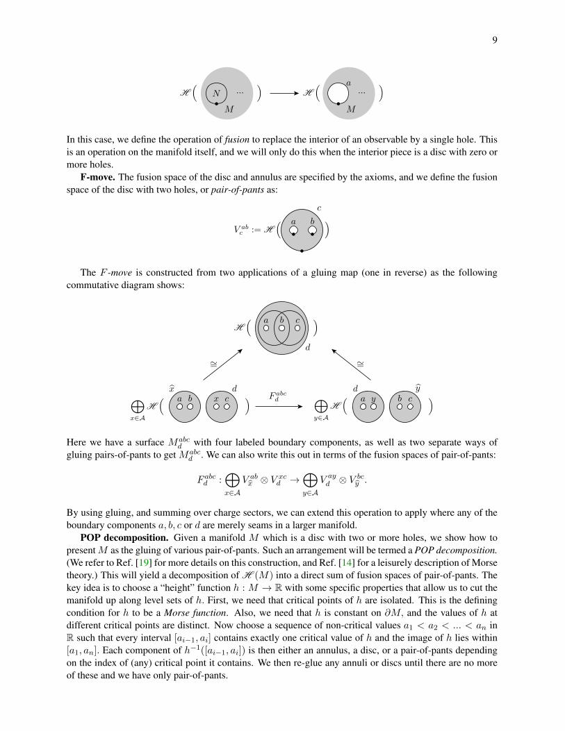
F-move. The fusion space of the disc and annulus are specified by the axioms, and we define the fusionspace of the disc with two holes, or pair-of-pants as:

V abc := H

( a b

c

)

The F -move is constructed from two applications of a gluing map (one in reverse) as the followingcommutative diagram shows:

a b c

d

H( )

a y b cyd

⊕

y∈AH

( )F abcda b x c

x d⊕

x∈AH

( )

∼= ∼=

Here we have a surface Mabcd with four labeled boundary components, as well as two separate ways of

gluing pairs-of-pants to get Mabcd . We can also write this out in terms of the fusion spaces of pair-of-pants:

F abcd :⊕

x∈AV abx ⊗ V xc

d →⊕

y∈AV ayd ⊗ V bc

y .

By using gluing, and summing over charge sectors, we can extend this operation to apply where any of theboundary components a, b, c or d are merely seams in a larger manifold.

POP decomposition. Given a manifold M which is a disc with two or more holes, we show how topresentM as the gluing of various pair-of-pants. Such an arrangement will be termed a POP decomposition.(We refer to Ref. [19] for more details on this construction, and Ref. [14] for a leisurely description of Morsetheory.) This will yield a decomposition of H (M) into a direct sum of fusion spaces of pair-of-pants. Thekey idea is to choose a “height” function h : M → R with some specific properties that allow us to cut themanifold up along level sets of h. First, we need that critical points of h are isolated. This is the definingcondition for h to be a Morse function. Also, we need that h is constant on ∂M, and the values of h atdifferent critical points are distinct. Now choose a sequence of non-critical values a1 < a2 < ... < an inR such that every interval [ai−1, ai] contains exactly one critical value of h and the image of h lies within[a1, an]. Each component of h−1([ai−1, ai]) is then either an annulus, a disc, or a pair-of-pants dependingon the index of (any) critical point it contains. We then re-glue any annuli or discs until there are no moreof these and we have only pair-of-pants.

10

Clearly such a POP decomposition is not unique, and the goal here is to understand how to switchbetween decompositions, and in particular, given an observable γ, and a given POP decomposition, find asequence of “moves” such that γ is in the resulting POP decomposition:

γ

One way to achieve this is via Cerf theory, which is the theory of how one may deform Morse functionsinto other Morse functions and the kind of transitions involved in their critical point structure. This was theapproach used in Ref. [6]. In this work we use a simpler method, which is essentially the same as skeintheory. This is the refactoring theorem that we describe below.

Dehn twist. Consider a surface Ma,a with two boundary components, a and a. Let f be a map Ma,a →Ma,a which performs a clockwise 2π full-twist or Dehn twist. Here we show the action of f by highlightingthe equator of the annulus:

a

af

a

a

We define the induced map on fusion spaces as θa := H (f). Because H (Ma,a) is one-dimensional thiswill be multiplication by a complex number which we also write as θa.

If we now takeM to be an arbitrary surface, and γ an observable onM,we can consider a neighbourhoodof γ which will be an annulus, and perform a Dehn twist there, which we denote as fγ : M →M. WritingM as a gluing along γ of another manifold Na,a, the action of H (fγ) will decompose as a direct sum overcharge sectors:

⊕

a∈AθaH (Na,a).

Standard surfaces. For each n = 0, 1, ... and every ordered sequence of anyon labels a1, ..., an, b wechoose a standard surface. This is a surface with n + 1 boundary components labeled a1, ..., an, b whichwe denote Ma1...an

b .For concreteness we define this surface using the following expression for a closed disc less n open

discs:{

(x, y) ∈ R2 st.∣∣∣(x, y)−

(1

2, 0)∣∣∣ ≤ 1

2

}−{

(x, y) ∈ R2 st.∣∣∣(x, y)−

(2i− 1

2n, 0)∣∣∣ < 1

4n

}i=1,...n

.

11

We then label the interior holes a1, ..., an in order of increasing x coordinate, and the exterior hole islabeled b. The base points are placed in the direction of negative y coordinate. As a notational conveniencewe highlight the equator of the surface which is the intersection of the x axis with the surface:

a1 ... an

b

Each standard surface comes with a collection of standard POP decompositions: these will be POPdecompositions where we require each observable to cross the equator twice and have counterclockwiseorientation. Up to isotopy, a given standard surface will have only finitely many of these. On a standardsurface with three interior holes there are two standard POP decompositions, and one F -move that relatesthese. On a standard surface with four interior holes there are five standard POP decompositions and fiveF -moves that relate these. In this case the F -moves themselves satisfy an equation that is an immediateconsequence of the way we have defined F -moves. This is known as the pentagon equation, which wedepict as the following commutative diagram:

F

F

F

F

F

We are now starting to confuse the notation for the topological spaceM and the fusion space H (M). Also,each of these F -moves is referring to an isomorphism that is block decomposed according to the chargesectors of the indicated observables.

We define the vector spaces V a1...anb := H (Ma1...an

b ). We now choose a basis for each of the V a1a2b

to be {va1a2b,µ }µ. For every standard POP decomposition of Ma1...anb , we get a decomposition of V a1...an

b

into direct sums of various V a′1a′2

b′ . This then gives a standard basis of V a1...anb relative to this standard POP

decomposition using the corresponding {va′1a′2

b′,µ }µ for each of the V a′1a′2

b′ .

Note that for any standard surface Ma1...anb and any choice of k contiguous holes aj , ..., aj+k−1 we can

find an observable that encloses exactly these holes in at least one of the standard POP decompositions ofMa1...anb .

We next show how to glue the exterior hole of a standard surface M to an interior hole of anotherstandard surface N. To do this within R2 we rescale and translate the two surfaces so that the exteriorhole of M coincides with the interior hole of N. At this point the union is not in general going to produce

12

another standard surface, and so we remedy this by applying any isotopy within R2 that fixes the x-axiswhile moving the surface to a standard surface.

Curve diagram. We next study maps from standard surfaces to arbitrary surfaces. The reader shouldthink of this as akin to choosing a basis for a vector space. The set of all maps from Ma1...an

b to a surfaceN will be denoted as Hom(Ma1...an

b , N). We call each such map a curve diagram, or more specifically, acurve diagram on N . The reason for this terminology is that we can reconstruct (up to isotopy) any mapf : Ma1...an

b → N from the restriction of f to the equator of Ma1...anb . In other words, we can uniquely

specify any map f : Ma1...anb → N by indicating the action of f on the equator. (This reconstruction

works because a simple closed curve on a sphere cuts the sphere into two discs.) We take full advantageof this fact in our notation: any figure of a surface with a “green line” drawn therein is actually notating adiffeomorphism, not a surface!

Any curve diagram will act on a standard POP decomposition of Ma1...anb sending it to a POP decom-

position of N. Surprisingly, the converse of this statement also holds: any POP decomposition of N (a discwith holes) comes from some curve diagram acting on a standard POP decomposition. The proof of this isconstructive, and we call this the refactoring theorem below.

The operation of gluing of surfaces can be extended to gluing of curve diagrams as long as we are carefulwith the way we identify along the seam: the identification map needs to respect the equator of the curvediagram. (Keep in mind that a curve diagram is really a map of surfaces, and so gluing two such mapsinvolves two separate gluing operations.)

We note in passing two connections to the mathematical literature. Such curve diagrams have been usedin the study of braid groups [20], and this is where the name comes from, although our curve diagramsrespect the base points and so could be further qualified as “framed” curve diagrams. And, we note thesimilarity of curve diagrams and associated modular functor to the definition of a planar algebra [21], themain difference being that planar algebras allow for not just two but any even number of curve intersectionsat each hole.

Z-move. We let z be a diffeomorphism of standard surfaces z : Ma1...anb →Ma2...anb

a1 that preserves theequator. (Considering the standard surface as a sphere with holes placed uniformly around a great circle, zis seen to be a “rotation”.) This acts by pre-composition to send a curve diagram f ∈ Hom(Ma1...an

b , N) tofz ∈ Hom(Ma2...anb

a1 , N). This we call a Z-move of f.In this way, any curve diagram can be seen as another curve diagram that has a cyclic permutation of the

labels of the underlying standard surface.R-move. Given anyon labels a, b and c, and arbitrary surface N, we now define the following map of

curve diagrams on N :

Rabc : Hom(Mabc , N)→ Hom(M ba

c , N).

This map works by taking a curve diagram f : Mabc → N to the composition fσ where σ : M ba

c →Mabc is

a counterclockwise “half-twist” map that exchanges the a and b holes. Here we show the action of Rabc onone particular curve diagram:

a

b

c

Rabc

b

a

c

Such an application of Rabc to a particular curve diagram we call an R-move. As noted above, a curvediagram serves to pick out a basis for the fusion space, and the point of this R-move is to switch betweendifferent curve diagrams for the same surface. This is highlighted to draw the readers attention to the factthat the R-move does not swap the labels on the holes: the surface itself stays the same.

13

As we extended Dehn twists under gluing, and F -moves under gluing, we also do this for R-moves.

Skeins. The previous figure can be seen as a “top-down” view of the following three dimensionalarrangement:

c

b a

Rabc

c

b a

This figure is intended to be topologically the same as the previous flat figure, with the addition of a thirddimension, and the c boundary has been shrunk. Also note thin black lines connecting the base points. Theblack lines do not add any extra structure, they can be seen as a part of the hexagon cut out by the greenline and boundary components. But notice this: the black lines are “framed” by the green lines. These arethe ribbons used in skein theory! Note that all the holes are created equal: there is no distinction between“input” holes and “output” holes (as there is with cobordisms or string diagrams.)

Hexagon equation. For a surface with three interior holes there are infinitely many POP decompositions(up to isotopy). These are all made by choosing an observable that encloses two holes. The F -movesallow us to switch between these POP decompositions, and the axioms for the modular functor make theseconsistent. Here we show two such triangle consistency requirements (they are reflections of each other):

F

F

F F

F

F

Given a POP decomposition of a surfaceN there are various curve diagrams onN that produce this decom-position from a standard POP decomposition, and there are certain R-moves that will map between these.Once again, these moves must be consistent, and here we note the two “hexagon equations” correspondingto the above two triangles:

14

R−1

F

R−1F

R

F F

R−1

FR

F

R

Note that we have neglected to indicate the base points here. Given a curve diagram, we can agree thatbase points occur “to the right” of the image of the equator. But in notating diagrams such as these, thereis still an ambiguity: the position of the base points should be the same in each surface in the diagram. Ifwe try to correct for this post-hoc by rotating individual holes, we will then be correct only up to possibleDehn twist(s) around each hole. We can certainly track these twists if we wanted to, but in the interests ofsimplicity we do not. This introduces a global phase ambiguity into the calculations.

The reason why we mention the pentagon and hexagon equations is that these become important in analgebraic description of the theory. Because we have defined everything in terms of a modular functor weget these equations “for free”.

C. Refactoring theorem

In this section we specialize to considering planar surfaces only. The theorem we are building towardsshows that the R-moves act transitively on curve diagrams. By transitive we mean that given two curvediagrams f and f ′ on N we can find a sequence of R-moves that transform f to f ′. The key idea is toconsider the (directed) image of the equator under these curve diagrams. As mentioned previously, thisimage is sufficient to define the entire diffeomorphism (up to isotopy) and so we are free to work with justthis image, or curve, and we confuse the distinction between a curve diagram (a diffeomorphism) and itscurve.

The construction proceeds by considering adjacent pairs of holes along f ′ and then acting on the portionof f between these same two holes so that they then become adjacent on the resulting curve. Continuingthis process for each two adjacent holes of f ′ will then show a sequence of R-moves that sends f to f ′.

To this end, consider a sequence of holes a1, ..., an appearing sequentially along f such that a1 and anappear sequentially on f ′. We may need to apply some Z-moves to f to ensure that a1 appears sequentiallybefore an. Now consider the case such that along f ′ between these two holes there is no intersection withf. We form a closed path ξ by following the f ′ curve between a1 and an and then following the f curve inreverse from an back to a1. (Note that to be completely rigorous here we would need to include segments ofpath contained within boundary components.) The resulting closed path bounds a disc. If ξ has clockwiseorientation we apply the following sequence of R-moves to f :

Ra1a2b1, Ra1a3b2

, ..., Ra1an−1

bn−1.

Depicted here is the first such move:

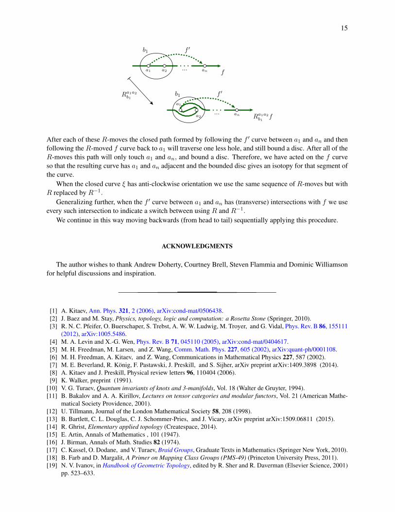
15

f

f ′

a1 a2 an...

b1

Ra1a2

b1

Ra1a2

b1f

f ′

a1

a2an...

b1

After each of these R-moves the closed path formed by following the f ′ curve between a1 and an and thenfollowing the R-moved f curve back to a1 will traverse one less hole, and still bound a disc. After all of theR-moves this path will only touch a1 and an, and bound a disc. Therefore, we have acted on the f curveso that the resulting curve has a1 and an adjacent and the bounded disc gives an isotopy for that segment ofthe curve.

When the closed curve ξ has anti-clockwise orientation we use the same sequence of R-moves but withR replaced by R−1.

Generalizing further, when the f ′ curve between a1 and an has (transverse) intersections with f we useevery such intersection to indicate a switch between using R and R−1.

We continue in this way moving backwards (from head to tail) sequentially applying this procedure.

ACKNOWLEDGMENTS

The author wishes to thank Andrew Doherty, Courtney Brell, Steven Flammia and Dominic Williamsonfor helpful discussions and inspiration.

[1] A. Kitaev, Ann. Phys. 321, 2 (2006), arXiv:cond-mat/0506438.[2] J. Baez and M. Stay, Physics, topology, logic and computation: a Rosetta Stone (Springer, 2010).[3] R. N. C. Pfeifer, O. Buerschaper, S. Trebst, A. W. W. Ludwig, M. Troyer, and G. Vidal, Phys. Rev. B 86, 155111

(2012), arXiv:1005.5486.[4] M. A. Levin and X.-G. Wen, Phys. Rev. B 71, 045110 (2005), arXiv:cond-mat/0404617.[5] M. H. Freedman, M. Larsen, and Z. Wang, Comm. Math. Phys. 227, 605 (2002), arXiv:quant-ph/0001108.[6] M. H. Freedman, A. Kitaev, and Z. Wang, Communications in Mathematical Physics 227, 587 (2002).[7] M. E. Beverland, R. Konig, F. Pastawski, J. Preskill, and S. Sijher, arXiv preprint arXiv:1409.3898 (2014).[8] A. Kitaev and J. Preskill, Physical review letters 96, 110404 (2006).[9] K. Walker, preprint (1991).

[10] V. G. Turaev, Quantum invariants of knots and 3-manifolds, Vol. 18 (Walter de Gruyter, 1994).[11] B. Bakalov and A. A. Kirillov, Lectures on tensor categories and modular functors, Vol. 21 (American Mathe-

matical Society Providence, 2001).[12] U. Tillmann, Journal of the London Mathematical Society 58, 208 (1998).[13] B. Bartlett, C. L. Douglas, C. J. Schommer-Pries, and J. Vicary, arXiv preprint arXiv:1509.06811 (2015).[14] R. Ghrist, Elementary applied topology (Createspace, 2014).[15] E. Artin, Annals of Mathematics , 101 (1947).[16] J. Birman, Annals of Math. Studies 82 (1974).[17] C. Kassel, O. Dodane, and V. Turaev, Braid Groups, Graduate Texts in Mathematics (Springer New York, 2010).[18] B. Farb and D. Margalit, A Primer on Mapping Class Groups (PMS-49) (Princeton University Press, 2011).[19] N. V. Ivanov, in Handbook of Geometric Topology, edited by R. Sher and R. Daverman (Elsevier Science, 2001)

pp. 523–633.

16

[20] P. Dehornoy, Why are braids orderable?, Panoramas et syntheses - Societe mathematique de France (SocieteMathematique de France, 2002).

[21] V. F. Jones, arXiv preprint math/9909027 (1999).