a short introduction to tensor analysiskokkotas/... · kostas kokkotas 9 a short introduction to...

A Short Introduction to Tensor Analysis

Kostas Kokkotas 2

February 19, 2018

2This chapter based strongly on “Lectures of General Relativity” by A. Papapetrou, D. Reidel publishing

company, (1974)

Kostas Kokkotas 3 A Short Introduction to Tensor Analysis

Scalars and Vectors

A n-dim manifold is a space M on every point of which we can assign nnumbers (x1,x2,...,xn) - the coordinates - in such a way that there will bean one to one correspondence between the points and the n numbers.

Every point of the manifold has itsown neighborhood which can bemapped to a n-dim Euclidean space.The manifold cannot be alwayscovered by a single system ofcoordinates and there is not apreferable one either.

The coordinates of the point P are connected by relations of the form:xµ

′= xµ

′ (x1, x2, ..., xn

)for µ′ = 1, ..., n and their inverse

xµ = xµ(x1′, x2′

, ..., xn′)

for µ = 1, ..., n. If there exist

Aµ′

ν =∂xµ

′

∂xνand Aνµ′ =

∂xν

∂xµ′ ⇒ det |Aµ′

ν | (1)

then the manifold is called differential.


Any physical quantity, e.g. the velocity of a particle, is determined by aset of numerical values - its components - which depend on thecoordinate system.

Tensors

Studying the way in which these values change with the coordinatesystem leads to the concept of tensor.

With the help of this concept we can express the physical laws by tensorequations, which have the same form in every coordinate system.

Scalar field : is any physical quantity determined by a singlenumerical value i.e. just one component which is independent of thecoordinate system (mass, charge,...)

Vector field (contravariant): an example is the infinitesimaldisplacement vector, leading from a point A with coordinates xµ toa neighbouring point A′ with coordinates xµ + dxµ. Thecomponents of such a vector are the differentials dxµ.


Any physical quantity, e.g. the velocity of a particle, is determined by aset of numerical values - its components - which depend on thecoordinate system.

Tensors

Studying the way in which these values change with the coordinatesystem leads to the concept of tensor.

With the help of this concept we can express the physical laws by tensorequations, which have the same form in every coordinate system.

Scalar field : is any physical quantity determined by a singlenumerical value i.e. just one component which is independent of thecoordinate system (mass, charge,...)

Vector field (contravariant): an example is the infinitesimaldisplacement vector, leading from a point A with coordinates xµ toa neighbouring point A′ with coordinates xµ + dxµ. Thecomponents of such a vector are the differentials dxµ.


company, (1974)


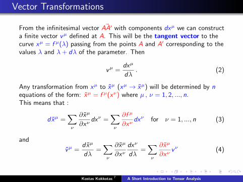
Vector Transformations

From the infinitesimal vector ~AA′ with components dxµ we can constructa finite vector vµ defined at A. This will be the tangent vector to thecurve xµ = f µ(λ) passing from the points A and A′ corresponding to thevalues λ and λ+ dλ of the parameter. Then

vµ =dxµ

dλ. (2)

Any transformation from xµ to xµ (xµ → xµ) will be determined by nequations of the form: xµ = f µ(xν) where µ , ν = 1, 2, ..., n.This means that :

dxµ =∑ν

∂xµ

∂xνdxν =

∑ν

∂f µ

∂xνdxν for ν = 1, ..., n (3)

and

vµ =dxµ

dλ=∑ν

∂xµ

∂xνdxν

dλ=∑ν

∂xµ

∂xνvν (4)


Contravariant and Covariant Vectors

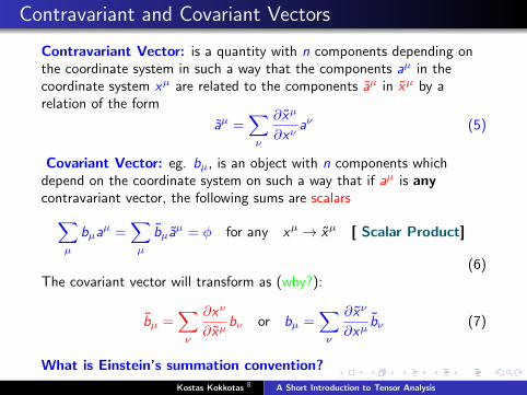
Contravariant Vector: is a quantity with n components depending onthe coordinate system in such a way that the components aµ in thecoordinate system xµ are related to the components aµ in xµ by arelation of the form

aµ =∑ν

∂xµ

∂xνaν (5)

Covariant Vector: eg. bµ, is an object with n components whichdepend on the coordinate system on such a way that if aµ is anycontravariant vector, the following sums are scalars∑

µ

bµaµ =

∑µ

bµaµ = φ for any xµ → xµ [ Scalar Product]

(6)The covariant vector will transform as (why?):

bµ =∑ν

∂xν

∂xµbν or bµ =

∑ν

∂xν

∂xµbν (7)

What is Einstein’s summation convention?


Tensors: at last

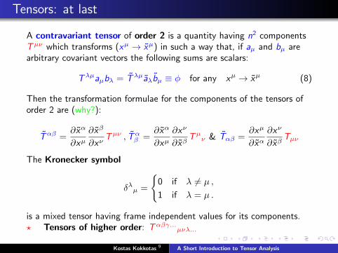
A contravariant tensor of order 2 is a quantity having n2 componentsTµν which transforms (xµ → xµ) in such a way that, if aµ and bµ arearbitrary covariant vectors the following sums are scalars:

Tλµaµbλ = Tλµaλbµ ≡ φ for any xµ → xµ (8)

Then the transformation formulae for the components of the tensors oforder 2 are (why?):

Tαβ =∂xα

∂xµ∂xβ

∂xνTµν , Tα

β =∂xα

∂xµ∂xν

∂xβTµ

ν & Tαβ =∂xµ

∂xα∂xν

∂xβTµν

The Kronecker symbol

δλµ =

{0 if λ 6= µ ,

1 if λ = µ .

is a mixed tensor having frame independent values for its components.? Tensors of higher order: Tαβγ...

µνλ...


Tensor algebra

Tensor addition : Tensors of the same order (p, q) can be added, theirsum being again a tensor of the same order. For example:

aν + bν =∂xν

∂xµ(aµ + bµ) (9)

Tensor multiplication : The product of two vectors is a tensor of order2, because

aαbβ =∂xα

∂xµ∂xβ

∂xνaµbν (10)

in general:

Tµν = AµBν or Tµν = AµBν or Tµν = AµBν (11)


Tensor algebra

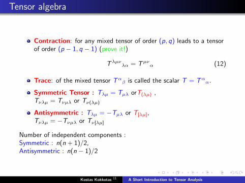
Contraction: for any mixed tensor of order (p, q) leads to a tensorof order (p − 1, q − 1) (prove it!)

Tλµνλα = Tµν

α (12)

Trace: of the mixed tensor Tαβ is called the scalar T = Tα

α.

Symmetric Tensor : Tλµ = Tµλ orT(λµ) ,Tνλµ = Tνµλ or Tν(λµ)

Antisymmetric : Tλµ = −Tµλ or T[λµ],Tνλµ = −Tνµλ or Tν[λµ]

Number of independent components :Symmetric : n(n + 1)/2,Antisymmetric : n(n − 1)/2


Tensors: Differentiation

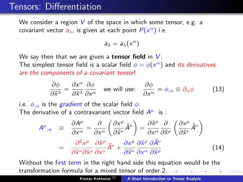
We consider a region V of the space in which some tensor, e.g. acovariant vector aλ, is given at each point P(xα) i.e.

aλ = aλ(xα)

We say then that we are given a tensor field in V .The simplest tensor field is a scalar field φ = φ(xα) and its derivativesare the components of a covariant tensor!

∂φ

∂xλ=∂xα

∂xλ∂φ

∂xαwe will use:

∂φ

∂xα= φ,α ≡ ∂αφ (13)

i.e. φ,α is the gradient of the scalar field φ.The derivative of a contravariant vector field Aµ is :

Aµ,α ≡ ∂Aµ

∂xα=

∂

∂xα

(∂xµ

∂xνAν)

=∂xρ

∂xα∂

∂xρ

(∂xµ

∂xνAν)

=∂2xµ

∂xν∂xρ∂xρ

∂xαAν +

∂xµ

∂xν∂xρ

∂xα∂Aν

∂xρ(14)

Without the first term in the right hand side this equation would be thetransformation formula for a mixed tensor of order 2.


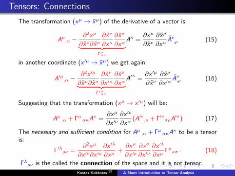
Tensors: Connections

The transformation (xµ → xµ) of the derivative of a vector is:

Aµ,α −∂2xµ

∂xν∂xσ∂xν

∂xκ∂xσ

∂xα︸︷︷︸Γµακ

Aκ =∂xµ

∂xν∂xρ

∂xαAν,ρ (15)

in another coordinate (x ′µ → xµ) we get again:

A′µ,α −∂2x ′µ

∂xν∂xσ∂xν

∂x ′κ∂xσ

∂xα︸︷︷︸Γ′µακ

A′κ

=∂x ′µ

∂xν∂xρ

∂x ′αAν,ρ (16)

Suggesting that the transformation (xµ → x ′µ) will be:

Aµ ,α + Γµ ακAκ =

∂xµ

∂x ′ν∂x ′ρ

∂xα(A′ν ,ρ + Γ′νσρA

′σ) (17)

The necessary and sufficient condition for Aµ ,α + Γµ ακAκ to be a tensor

is:

Γ′λρν =∂2xµ

∂x ′ν∂x ′ρ∂x ′λ

∂xµ+∂xκ

∂x ′ρ∂xσ

∂x ′ν∂x ′λ

∂xµΓµκσ . (18)

Γλρν is the called the connection of the space and it is not tensor.


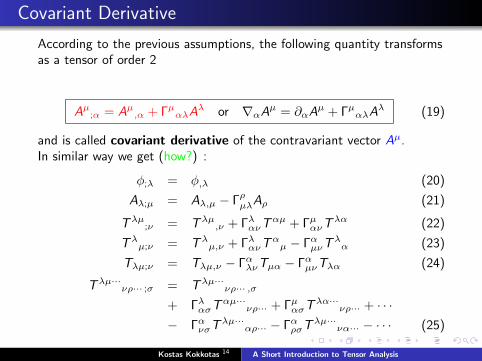
Covariant Derivative

According to the previous assumptions, the following quantity transformsas a tensor of order 2

Aµ;α = Aµ,α + ΓµαλAλ or ∇αAµ = ∂αA

µ + ΓµαλAλ (19)

and is called covariant derivative of the contravariant vector Aµ.In similar way we get (how?) :

φ;λ = φ,λ (20)

Aλ;µ = Aλ,µ − ΓρµλAρ (21)

Tλµ;ν = Tλµ

,ν + ΓλανTαµ + ΓµανT

λα (22)

Tλµ;ν = Tλ

µ,ν + ΓλανTαµ − ΓαµνT

λα (23)

Tλµ;ν = Tλµ,ν − ΓαλνTµα − ΓαµνTλα (24)

Tλµ···νρ··· ;σ = Tλµ···

νρ··· ,σ

+ ΓλασTαµ···

νρ··· + ΓµασTλα···

νρ··· + · · ·− ΓανσT

λµ···αρ··· − ΓαρσT

λµ···να··· − · · · (25)


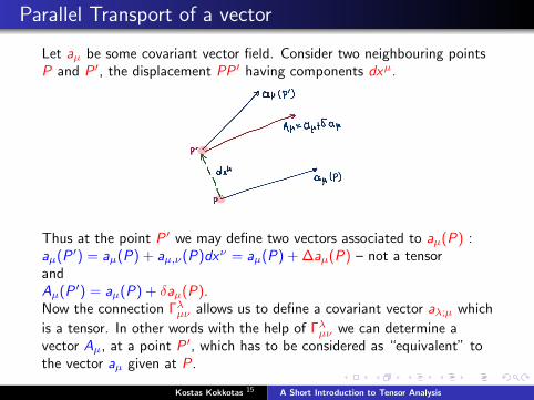
Parallel Transport of a vector

Let aµ be some covariant vector field. Consider two neighbouring pointsP and P ′, the displacement PP ′ having components dxµ.

Thus at the point P ′ we may define two vectors associated to aµ(P) :aµ(P ′) = aµ(P) + aµ,ν(P)dxν = aµ(P) + ∆aµ(P) – not a tensorandAµ(P ′) = aµ(P) + δaµ(P).Now the connection Γλµν allows us to define a covariant vector aλ;µ which

is a tensor. In other words with the help of Γλµν we can determine avector Aµ, at a point P ′, which has to be considered as “equivalent” tothe vector aµ given at P.


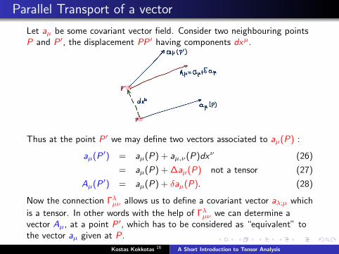
Parallel Transport of a vector

Let aµ be some covariant vector field. Consider two neighbouring pointsP and P ′, the displacement PP ′ having components dxµ.

Thus at the point P ′ we may define two vectors associated to aµ(P) :

aµ(P ′) = aµ(P) + aµ,ν(P)dxν (26)

= aµ(P) + ∆aµ(P) not a tensor (27)

Aµ(P ′) = aµ(P) + δaµ(P). (28)

Now the connection Γλµν allows us to define a covariant vector aλ;µ which

is a tensor. In other words with the help of Γλµν we can determine avector Aµ, at a point P ′, which has to be considered as “equivalent” tothe vector aµ given at P.


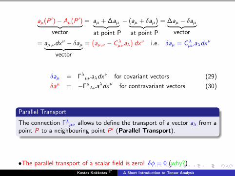
aµ(P ′)− Aµ(P ′)︸︷︷︸vector

= aµ + ∆aµ︸︷︷︸at point P

− (aµ + δaµ)︸︷︷︸at point P

= ∆aµ − δaµ︸︷︷︸vector

= aµ,νdxν − δaµ︸︷︷︸

vector

=(aµ,ν − Cλµνaλ

)dxν i.e. δaµ = Cλµνaλdx

ν

δaµ = Γλµνaλdxν for covariant vectors (29)

δaµ = −Γµλνaλdxν for contravariant vectors (30)

Parallel Transport

The connection Γλµν allows to define the transport of a vector aλ from apoint P to a neighbouring point P ′ (Parallel Transport).

•The parallel transport of a scalar field is zero! δφ = 0 (why?)


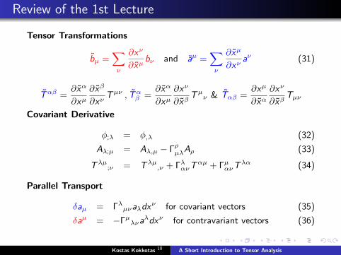
Review of the 1st Lecture

Tensor Transformations

bµ =∑ν

∂xν

∂xµbν and aµ =

∑ν

∂xµ

∂xνaν (31)

Tαβ =∂xα

∂xµ∂xβ

∂xνTµν , Tα

β =∂xα

∂xµ∂xν

∂xβTµ

ν & Tαβ =∂xµ

∂xα∂xν

∂xβTµν

Covariant Derivative

φ;λ = φ,λ (32)

Aλ;µ = Aλ,µ − ΓρµλAρ (33)

Tλµ;ν = Tλµ

,ν + ΓλανTαµ + ΓµανT

λα (34)

Parallel Transport

δaµ = Γλµνaλdxν for covariant vectors (35)

δaµ = −Γµλνaλdxν for contravariant vectors (36)


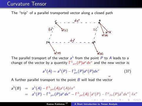
Curvature Tensor

The “trip” of a parallel transported vector along a closed path

The parallel transport of the vector aλ from the point P to A leads to achange of the vector by a quantity Γλµν(P)aµdxν and the new vector is:

aλ(A) = aλ(P)− Γλµν(P)aµ(P)dxν (37)

A further parallel transport to the point B will lead the vector

aλ(B) = aλ(A)− Γλρσ(A)aρ(A)δxσ

= aλ(P)− Γλµν(P)aµdxν − Γλρσ(A)[aρ(P)− Γρβν(P)aβdxν

]δxσ


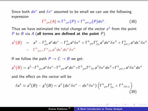
Since both dxν and δxν assumed to be small we can use the followingexpression

Γλρσ(A) ≈ Γλρσ(P) + Γλρσ,µ(P)dxµ . (38)

Thus we have estimated the total change of the vector aλ from the pointP to B via A (all terms are defined at the point P).

aλ(B) = aλ − Γλµνaµdxν − Γλρσa

ρδxσ + ΓλρσΓρβνaβdxνδxβ + Γλρσ,τa

ρdxτδxσ

− Γλρσ,τΓρβνaβdxτdxνδxσ

If we follow the path P → C → B we get:

aλ(B) = aλ−Γλµνaµδxν−Γλρσa

ρdxσ+ΓλρσΓρβνaβδxνdxβ+Γλρσ,τa

ρδxτdxσ

and the effect on the vector will be

δaλ ≡ aλ(B)− aλ(B) = aβ (dxνδxσ − dxσδxν)(

ΓλρσΓρβν + Γλβσ,ν)(39)


By exchanging the indices ν → σ and σ → ν we construct a similarrelation

δaλ = aβ (dxσδxν − dxνδxσ)(ΓλρνΓρβσ + Γλβν,σ

)(40)

and the total change will be given by the following relation:

δaλ = −1

2aβRλβνσ (dxσδxν − dxνδxσ) (41)

where

Rλβνσ = −Γλβν,σ + Γλβσ,ν − ΓµβνΓλµσ + ΓµβσΓλµν (42)

is the curvature tensor.

Figure: Measuring the curvature for the space.


Geodesics

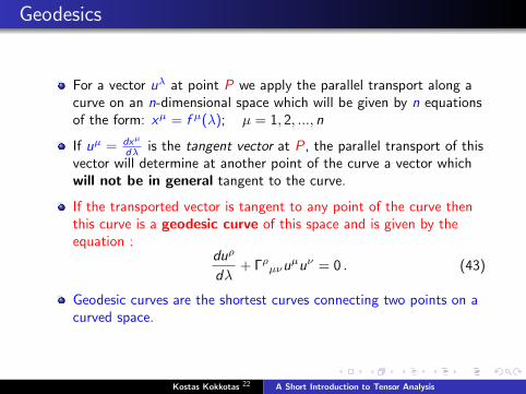
For a vector uλ at point P we apply the parallel transport along acurve on an n-dimensional space which will be given by n equationsof the form: xµ = f µ(λ); µ = 1, 2, ..., n

If uµ = dxµ

dλ is the tangent vector at P, the parallel transport of thisvector will determine at another point of the curve a vector whichwill not be in general tangent to the curve.

If the transported vector is tangent to any point of the curve thenthis curve is a geodesic curve of this space and is given by theequation :

duρ

dλ+ Γρµνu

µuν = 0 . (43)

Geodesic curves are the shortest curves connecting two points on acurved space.


Metric Tensor

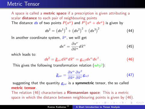
A space is called a metric space if a prescription is given attributing ascalar distance to each pair of neighbouring pointsThe distance ds of two points P(xµ) and P ′(xµ + dxµ) is given by

ds2 =(dx1)2

+(dx2)2

+(dx3)2

(44)

In another coordinate system, xµ, we will get

dxν =∂xν

∂xαdxα (45)

which leads to:ds2 = gµνdx

µdxν = gαβdxαdxβ . (46)

This gives the following transformation relation (why?):

gµν =∂xα

∂xµ∂xβ

∂xνgαβ (47)

suggesting that the quantity gµν is a symmetric tensor, the so calledmetric tensor.The relation (46) characterises a Riemannian space: This is a metricspace in which the distance between neighbouring points is given by (46).


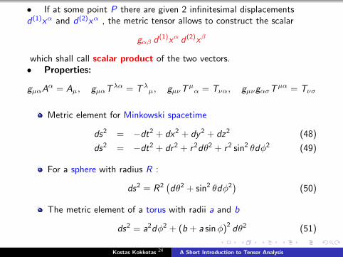
• If at some point P there are given 2 infinitesimal displacementsd (1)xα and d (2)xα , the metric tensor allows to construct the scalar

gαβ d(1)xα d (2)xβ

which shall call scalar product of the two vectors.• Properties:

gµαAα = Aµ, gµαT

λα = Tλµ, gµνT

µα = Tνα, gµνgασT

µα = Tνσ

Metric element for Minkowski spacetime

ds2 = −dt2 + dx2 + dy2 + dz2 (48)

ds2 = −dt2 + dr2 + r2dθ2 + r2 sin2 θdφ2 (49)

For a sphere with radius R :

ds2 = R2(dθ2 + sin2 θdφ2

)(50)

The metric element of a torus with radii a and b

ds2 = a2dφ2 + (b + a sinφ)2 dθ2 (51)


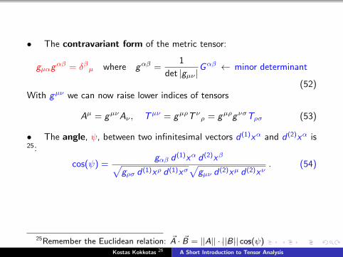
• The contravariant form of the metric tensor:

gµαgαβ = δβµ where gαβ =

1

det |gµν |Gαβ ← minor determinant

(52)With gµν we can now raise lower indices of tensors

Aµ = gµνAν , Tµν = gµρT νρ = gµρgνσTρσ (53)

• The angle, ψ, between two infinitesimal vectors d (1)xα and d (2)xα is25:

cos(ψ) =gαβ d

(1)xα d (2)xβ√gρσ d (1)xρ d (1)xσ

√gµν d (2)xµ d (2)xν

. (54)

25Remember the Euclidean relation: ~A · ~B = ||A|| · ||B|| cos(ψ)Kostas Kokkotas 26 A Short Introduction to Tensor Analysis

The Determinant of gµν

The quantity g ≡ det |gµν | is the determinant of the metric tensor. Thedeterminant transforms as :

g = det gµν = det

(gαβ

∂xα

∂xµ∂xβ

∂xν

)= det gαβ · det

(∂xα

∂xµ

)· det

(∂xβ

∂xν

)=

(det

∂xα

∂xµ

)2

g = J 2g (55)

where J is the Jacobian of the transformation.This relation can be written also as:√

|g | = J√|g | (56)

i.e. the quantity√|g | is a scalar density of weight 1.

• The quantity √|g |δV ≡

√|g |dx1dx2 . . . dxn (57)

is the invariant volume element of the Riemannian space.• If the determinant vanishes at a point P the invariant volume is zeroand this point will be called a singular point.


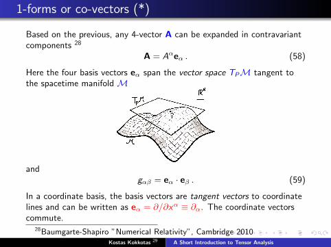
1-forms or co-vectors (*)

Based on the previous, any 4-vector A can be expanded in contravariantcomponents 28

A = Aαeα . (58)

Here the four basis vectors eα span the vector space TPM tangent tothe spacetime manifold M

andgαβ = eα · eβ . (59)

In a coordinate basis, the basis vectors are tangent vectors to coordinatelines and can be written as eα = ∂/∂xα ≡ ∂α. The coordinate vectorscommute.

28Baumgarte-Shapiro ”Numerical Relativity”, Cambridge 2010Kostas Kokkotas 29 A Short Introduction to Tensor Analysis

We may also set an orthonormal basis vectors at a point (orthonormaltetrad) for which

eα · eβ = ηαβ . (60)

• In general, orthonormal basis vectors do not form a coordinate basisand do not commute.• In a flat spacetime it is always possible to transform to coordinateswhich are everywhere orthonormal i.e. ηαβ = diag(−1, 1, 1, 1).• For a genaral spacetime this is not possible, but one may selectan event in the spacetime to be the origin of a local inertial coordinateframe, where gαβ = ηαβ at this point and in addition the 1st derivativesof the metric tensor at that point vanish, i.e. ∂γgαβ = 0.• An observer in such a coordinate frame is called a local inertial andcan use a coordinate basis that forms that forms a local orthonormaltetrad to make measurements in SR.• Such n observer will find that all the (non-gravitational) laws ofphysics in this frame are the same as in special relativity.• The scalar product of two 4-vectors A and B is

A · B = (Aαeα) ·(Bβeβ

)= gαβA

αBβ . (61)


1-forms (*)

• A 1-form can be defined as a linear, real valued function of vectors. 31

• A 1-form ω at a point P associates with a vector v at P a realnumber, which maybe called ω(v). We may say that ω is a function ofvectors while the linearity of this function means:

ω(av + bw) = aω(v) + bω(w) a, b ∈ IR

(aω)(v) = a[ω(v)]

(ω + σ) (v) = ω(v) + σ(v)

• Thus 1-forms at a point P satisfy the axioms of a vector space, whichis called the dual space to TP , and is denoted by T ∗P .• The linearity also allows to consider the vector as function of 1-forms:Thus vectors and 1-forms are thus said to be dual to each other.• Their value on one another can be represented as follows:

ω(v) ≡ v(ω) ≡< ω, v > . (62)

31See B. F. Schutz “Geometrical methods of mathematical physics”Cambridge, 1980.


1-forms (*)

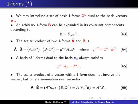
• We may introduce a set of basis 1-forms ωα dual to the basis vectorseα.• An arbitrary 1-form B can be expanded in its covariant componentsaccording to

B = Bαωα . (63)

• The scalar product of two 1-forms A and B is

A · B = (Aαωα) ·

(Bβω

β)

= gαβAαBβ where gαβ = ωα · ωβ . (64)

• A basis of 1-forms dual to the basis eα always satisfies

ωα · eβ = δαβ . (65)

• The scalar product of a vector with a 1-form does not involve themetric, but only a summation over an index

A · B = (Aαeα) ·(Bβω

β)

= AαδαβBβ = AαBα . (66)


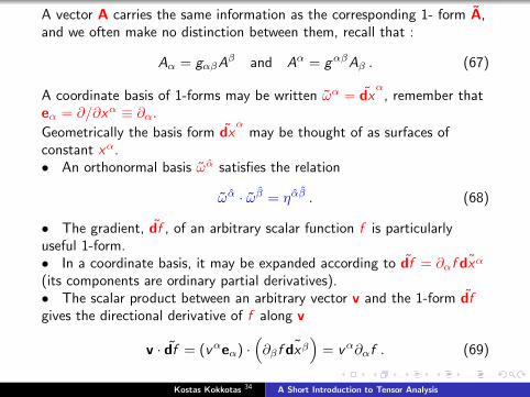
A vector A carries the same information as the corresponding 1- form A,and we often make no distinction between them, recall that :

Aα = gαβAβ and Aα = gαβAβ . (67)

A coordinate basis of 1-forms may be written ωα = dxα

, remember thateα = ∂/∂xα ≡ ∂α.

Geometrically the basis form dxα

may be thought of as surfaces ofconstant xα.• An orthonormal basis ωα satisfies the relation

ωα · ωβ = ηαβ . (68)

• The gradient, df , of an arbitrary scalar function f is particularlyuseful 1-form.• In a coordinate basis, it may be expanded according to df = ∂αf ˜dxα

(its components are ordinary partial derivatives).• The scalar product between an arbitrary vector v and the 1-form dfgives the directional derivative of f along v

v · df = (vαeα) ·(∂βf ˜dxβ

)= vα∂αf . (69)


Christoffel Symbols

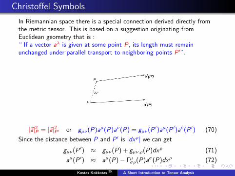
In Riemannian space there is a special connection derived directly fromthe metric tensor. This is based on a suggestion originating fromEuclidean geometry that is :“ If a vector aλ is given at some point P, its length must remainunchanged under parallel transport to neighboring points P ′”.

|~a|2P = |~a|2P′ or gµν(P)aµ(P)aν(P) = gµν(P ′)aµ(P ′)aν(P ′) (70)

Since the distance between P and P ′ is |dxρ| we can get

gµν(P ′) ≈ gµν(P) + gµν,ρ(P)dxρ (71)

aµ(P ′) ≈ aµ(P)− Γµσρ(P)aσ(P)dxρ (72)


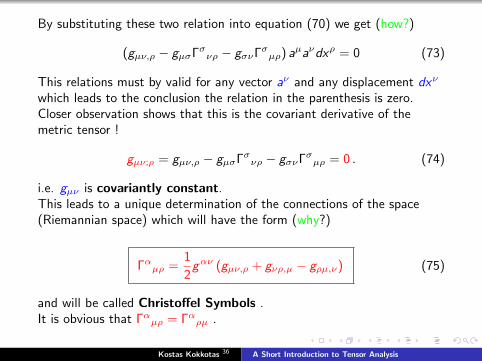
By substituting these two relation into equation (70) we get (how?)

(gµν,ρ − gµσΓσνρ − gσνΓσµρ) aµaνdxρ = 0 (73)

This relations must by valid for any vector aν and any displacement dxν

which leads to the conclusion the relation in the parenthesis is zero.Closer observation shows that this is the covariant derivative of themetric tensor !

gµν;ρ = gµν,ρ − gµσΓσνρ − gσνΓσµρ = 0 . (74)

i.e. gµν is covariantly constant.This leads to a unique determination of the connections of the space(Riemannian space) which will have the form (why?)

Γαµρ =1

2gαν (gµν,ρ + gνρ,µ − gρµ,ν) (75)

and will be called Christoffel Symbols .It is obvious that Γαµρ = Γαρµ .


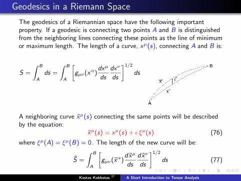
Geodesics in a Riemann Space

The geodesics of a Riemannian space have the following importantproperty. If a geodesic is connecting two points A and B is distinguishedfrom the neighboring lines connecting these points as the line of minimumor maximum length. The length of a curve, xµ(s), connecting A and B is:

S =

∫ B

A

ds =

∫ B

A

[gµν(xα)

dxµ

ds

dxν

ds

]1/2

ds

A neighboring curve xµ(s) connecting the same points will be describedby the equation:

xµ(s) = xµ(s) + ε ξµ(s) (76)

where ξµ(A) = ξµ(B) = 0. The length of the new curve will be:

S =

∫ B

A

[gµν(xα)

dxµ

ds

dxν

ds

]1/2

ds (77)


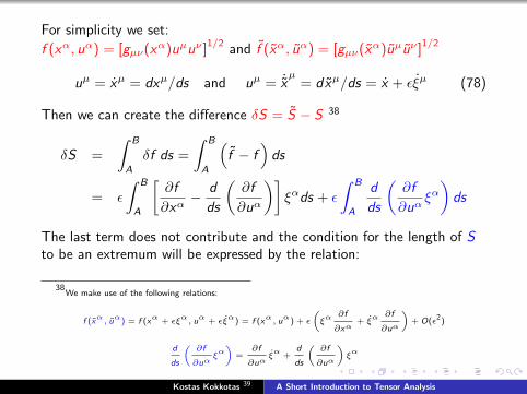
For simplicity we set:

f (xα, uα) = [gµν(xα)uµuν ]1/2 and f (xα, uα) = [gµν(xα)uµuν ]1/2

uµ = xµ = dxµ/ds and uµ = ˙xµ

= dxµ/ds = x + εξµ (78)

Then we can create the difference δS = S − S 38

δS =

∫ B

A

δf ds =

∫ B

A

(f − f

)ds

= ε

∫ B

A

[∂f

∂xα− d

ds

(∂f

∂uα

)]ξαds + ε

∫ B

A

d

ds

(∂f

∂uαξα)ds

The last term does not contribute and the condition for the length of Sto be an extremum will be expressed by the relation:

38We make use of the following relations:

f (xα, uα) = f (xα + εξα, uα + εξ

α) = f (xα, uα) + ε

(ξα ∂f

∂xα+ ξ

α ∂f

∂uα

)+ O(ε2)

d

ds

(∂f

∂uαξα)

=∂f

∂uαξα +

d

ds

(∂f

∂uα

)ξα


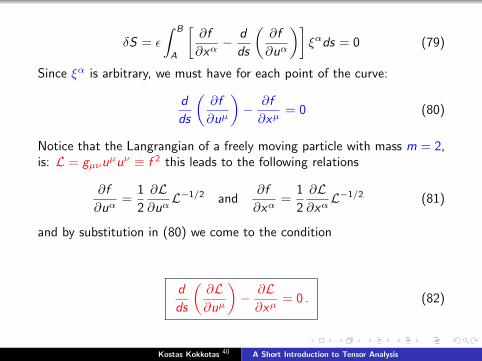
δS = ε

∫ B

A

[∂f

∂xα− d

ds

(∂f

∂uα

)]ξαds = 0 (79)

Since ξα is arbitrary, we must have for each point of the curve:

d

ds

(∂f

∂uµ

)− ∂f

∂xµ= 0 (80)

Notice that the Langrangian of a freely moving particle with mass m = 2,is: L = gµνu

µuν ≡ f 2 this leads to the following relations

∂f

∂uα=

1

2

∂L∂uαL−1/2 and

∂f

∂xα=

1

2

∂L∂xαL−1/2 (81)

and by substitution in (80) we come to the condition

d

ds

(∂L∂uµ

)− ∂L∂xµ

= 0 . (82)


Since L = gµνuµuν we get:

∂L∂uα

= gµν∂uµ

∂uαuν + gµνu

µ ∂uν

∂uα= gµνδ

µαuν + gµνu

µδνα = 2gµαuµ (83)

∂L∂xα

= gµν,αuµuν (84)

thus

d

ds(2gµαu

µ) = 2dgµαds

uµ + 2gµαduµ

ds= 2gµα,νu

νuµ + 2gµαduµ

ds

= gµα,νuνuµ + gνα,µu

µuν + 2gµαduµ

ds(85)

and by substitution (84) and (85) in (82) we get

gµαduµ

ds+

1

2[gµα,ν + gαµ,ν − gµν,α] uµuν = 0

if we multiply with gρα the geodesic equations

duρ

ds+ Γρµνu

µuν = 0 , or uρ;νuν = 0 (86)

because duρ/ds = uρ,µuµ.


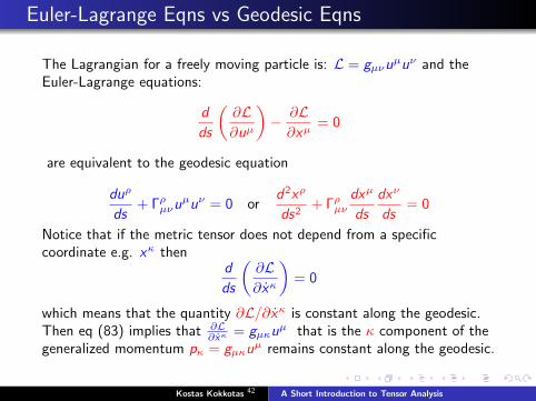
Euler-Lagrange Eqns vs Geodesic Eqns

The Lagrangian for a freely moving particle is: L = gµνuµuν and the

Euler-Lagrange equations:

d

ds

(∂L∂uµ

)− ∂L∂xµ

= 0

are equivalent to the geodesic equation

duρ

ds+ Γρµνu

µuν = 0 ord2xρ

ds2+ Γρµν

dxµ

ds

dxν

ds= 0

Notice that if the metric tensor does not depend from a specificcoordinate e.g. xκ then

d

ds

(∂L∂xκ

)= 0

which means that the quantity ∂L/∂xκ is constant along the geodesic.Then eq (83) implies that ∂L

∂xκ = gµκuµ that is the κ component of the

generalized momentum pκ = gµκuµ remains constant along the geodesic.


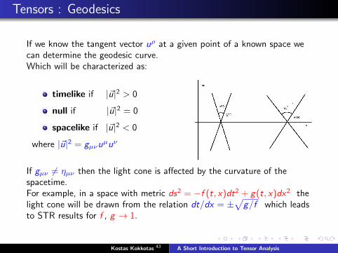
Tensors : Geodesics

If we know the tangent vector uρ at a given point of a known space wecan determine the geodesic curve.Which will be characterized as:

timelike if |~u|2 > 0

null if |~u|2 = 0

spacelike if |~u|2 < 0

where |~u|2 = gµνuµuν

If gµν 6= ηµν then the light cone is affected by the curvature of thespacetime.For example, in a space with metric ds2 = −f (t, x)dt2 + g(t, x)dx2 thelight cone will be drawn from the relation dt/dx = ±

√g/f which leads

to STR results for f , g → 1.


Null Geodesics

For null geodesics ds = 0 and the proper length s cannot be used toparametrize the geodesic curves. Instead we will use another parameter λand the equations will be written as:

d2xκ

dλ2+ Γκµν

dxµ

dλ

dxν

dλ= 0 (87)

and obiously:

gµνdxµ

dλ

dxν

dλ= 0 . (88)


Geodesic Eqns & Affine Parameter

In deriving the geodesic equations we have chosen to parametrize thecurve via the proper length s. This choice simplifies the form of theequation but it is not a unique choice. If we chose a new parameter, σthen the geodesic equations will be written:

d2xµ

dσ2+ Γµαβ

dxα

dσ

dxβ

dσ= − d2σ/ds2

(dσ/ds)2

dxµ

dσ(89)

where we have used

dxµ

ds=

dxµ

dσ

dσ

dsand

d2xµ

ds2=

d2xµ

dσ2

(dσ

ds

)2

+dxµ

dσ

d2σ

ds2(90)

The new geodesic equation (89), reduces to the original equation(87)when the right hand side is zero. This is possible if

d2σ

ds2= 0 (91)

which leads to a linear relation between s and σ i.e. σ = αs + β where αand β are arbitrary constants. σ is called affine parameter.


Riemann Tensor

When in a space we define a metric then is called metric space orRiemann space. For such a space the curvature tensor

Rλβνµ = −Γλβν,µ + Γλβµ,ν − ΓσβνΓλσµ + ΓσβµΓλσν (92)

is called Riemann Tensor and can be also written as:

Rκβνµ = gκλRλβνµ =

1

2(gκµ,βν + gβν,κµ − gκν,βµ − gβµ,κν)

+ gαρ(

ΓακµΓρβν − ΓακνΓρβµ

)Properties of the Riemann Tensor:

Rκβνµ = −Rκβµν , Rκβνµ = −Rβκνµ , Rκβνµ = Rνµκβ , Rκ[βµν] = 0

Thus in an n-dim space the number of independent components is(how?):

n2(n2 − 1)/12 (93)

For a 4-dimensional space only 20 independent components


The Ricci and Einstein Tensors

The contraction of the Riemann tensor leads to Ricci Tensor

Rαβ = Rλαλβ = gλµRλαµβ

= Γµαβ,µ − Γµαµ,β + ΓµαβΓννµ − ΓµανΓνβµ (94)

which is symmetric i.e. Rαβ = Rβα.Further contraction leads to the Ricci or Curvature Scalar

R = Rαα = gαβRαβ = gαβgµνRµανβ . (95)

The following combination of Riemann and Ricci tensors is calledEinstein Tensor

Gµν = Rµν −1

2gµνR (96)

with the very important property:

Gµν;µ =

(Rµν −

1

2δµνR

);µ

= 0 . (97)

This results from the Bianchi Identity (how?)

Rλµ[νρ;σ] = 0 (98)


Flat & Empty Spacetimes

When Rαβµν = 0 the spacetime is flat

When Rµν = 0 the spacetime is empty

Prove that :aλ;µ;ν − aλ;ν;µ = −Rλκµνaκ


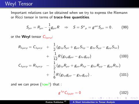
Weyl Tensor

Important relations can be obtained when we try to express the Riemannor Ricci tensor in terms of trace-free quantities.

Sµν = Rµν −1

4gµνR ⇒ S = Sµµ = gµνSµν = 0 . (99)

or the Weyl tensor Cλµνρ:

Rλµνρ = Cλµνρ +1

2(gλρSµν + gµνSλρ − gλνSµρ − gµρSλν)

+1

12R (gλρgµν − gλνgµρ) (100)

Cλµνρ = Rλµνρ − 1

2(gλρRµν + gµνRλρ − gλνRµρ − gµρRλν)

+1

6R (gλρgµν − gλνgµρ) . (101)

and we can prove (how?) that :

gλρCλµρν = 0 (102)


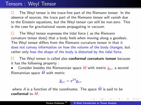
Tensors : Weyl Tensor

� The Weyl tensor is the trace-free part of the Riemann tensor. In theabsence of sources, the trace part of the Riemann tensor will vanish dueto the Einstein equations, but the Weyl tensor can still be non-zero. Thisis the case for gravitational waves propagating in vacuum.

� The Weyl tensor expresses the tidal force ( as the Riemanncurvature tensor does) that a body feels when moving along a geodesic.The Weyl tensor differs from the Riemann curvature tensor in that itdoes not convey information on how the volume of the body changes, butrather only how the shape of the body is distorted by the tidal force.

� The Weyl tensor is called also conformal curvature tensor becauseit has the following property :• Consider besides the Riemannian space M with metric gµν a second

Riemannian space M with metric

gµν = e2Agµν

where A is a function of the coordinates. The space M is said to beconformal to M.


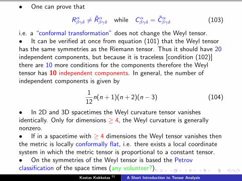
• One can prove that

Rαβγδ 6= Rαβγδ while Cαβγδ = Cαβγδ (103)

i.e. a “conformal transformation” does not change the Weyl tensor.• It can be verified at once from equation (101) that the Weyl tensorhas the same symmetries as the Riemann tensor. Thus it should have 20independent components, but because it is traceless [condition (102)]there are 10 more conditions for the components therefore the Weyltensor has 10 independent components. In general, the number ofindependent components is given by

1

12n(n + 1)(n + 2)(n − 3) (104)

• In 2D and 3D spacetimes the Weyl curvature tensor vanishesidentically. Only for dimensions ≥ 4, the Weyl curvature is generallynonzero.• If in a spacetime with ≥ 4 dimensions the Weyl tensor vanishes thenthe metric is locally conformally flat, i.e. there exists a local coordinatesystem in which the metric tensor is proportional to a constant tensor.• On the symmetries of the Weyl tensor is based the Petrovclassification of the space times (any volunteer?).


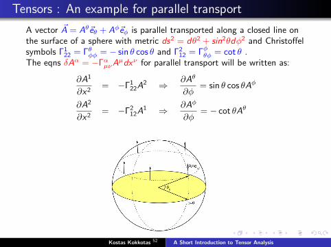
Tensors : An example for parallel transport

A vector ~A = Aθ~eθ + Aφ~eφ is parallel transported along a closed line onthe surface of a sphere with metric ds2 = dθ2 + sin2θdφ2 and Christoffelsymbols Γ1

22 = Γθφφ = − sin θ cos θ and Γ212 = Γφθφ = cot θ .

The eqns δAα = −ΓαµνAµdxν for parallel transport will be written as:

∂A1

∂x2= −Γ1

22A2 ⇒ ∂Aθ

∂φ= sin θ cos θAφ

∂A2

∂x2= −Γ2

12A1 ⇒ ∂Aφ

∂φ= − cot θAθ


The solutions will be:

∂2Aθ

∂φ2= − cos2 θAθ ⇒ Aθ = α cos(φ cos θ) + β sin(φ cos θ)

⇒ Aφ = − [α sin(φ cos θ)− β cos(φ cos θ)] sin−1 θ

and for an initial unit vector (Aθ,Aφ) = (1, 0) at (θ, φ) = (θ0, 0) theintegration constants will be α = 1 and β = 0.

The solution is:

~A = Aθ~eθ + Aφ~eφ = cos(2π cos θ)~eθ −sin(2π cos θ)

sin θ~eφ

i.e. different components but the measure is still the same

|~A|2 = gµνAµAν =

(Aθ)2

+ sin2 θ(Aφ)2

= cos2(2π cos θ) + sin2 θsin2(2π cos θ)

sin2 θ= 1

Question : What is the condition for the path followed by the vector tobe a geodesic?


The solutions will be:

∂2Aθ

∂φ2= − cos2 θAθ ⇒ Aθ = α cos(φ cos θ) + β sin(φ cos θ)

⇒ Aφ = − [α sin(φ cos θ)− β cos(φ cos θ)] sin−1 θ

and for an initial unit vector (Aθ,Aφ) = (1, 0) at (θ, φ) = (θ0, 0) theintegration constants will be α = 1 and β = 0.

The solution is:

~A = Aθ~eθ + Aφ~eφ = cos(2π cos θ)~eθ −sin(2π cos θ)

sin θ~eφ

i.e. different components but the measure is still the same

|~A|2 = gµνAµAν =

(Aθ)2

+ sin2 θ(Aφ)2

= cos2(2π cos θ) + sin2 θsin2(2π cos θ)

sin2 θ= 1

Question : What is the condition for the path followed by the vector tobe a geodesic?


company, (1974)Kostas Kokkotas 54 A Short Introduction to Tensor Analysis

a short introduction to tensor analysiskokkotas/... · kostas kokkotas 9 a short introduction to...

Documents