a short tutorial on using metax for high-throughput mass...

A short tutorial on using metaX for high-throughput massspectrometry-based metabolomic data analysis

Bo Wen

May 15, 2016

Contents

1 Introduction 2

2 Example data 2

3 Using metaX 23.1 Data import . . . . . . . . . . . . . . . . . . . . . . . . . . . . . . . . . . . . . . . . 2

3.1.1 Input compound intensity table file . . . . . . . . . . . . . . . . . . . . . . . . 23.1.2 Input MS data files . . . . . . . . . . . . . . . . . . . . . . . . . . . . . . . . 4

3.2 Integrated function metaXpipe() . . . . . . . . . . . . . . . . . . . . . . . . . . . . . 63.3 Function modules . . . . . . . . . . . . . . . . . . . . . . . . . . . . . . . . . . . . . 7

3.3.1 Peak picking and annotation . . . . . . . . . . . . . . . . . . . . . . . . . . . . 73.3.2 Missing value imputation . . . . . . . . . . . . . . . . . . . . . . . . . . . . . 73.3.3 Normalization . . . . . . . . . . . . . . . . . . . . . . . . . . . . . . . . . . . 83.3.4 Pre-processing of raw peak data . . . . . . . . . . . . . . . . . . . . . . . . . . 93.3.5 Removal of outliers . . . . . . . . . . . . . . . . . . . . . . . . . . . . . . . . 93.3.6 Power analysis and sample size estimation . . . . . . . . . . . . . . . . . . . . 93.3.7 Metabolite correlation network analysis . . . . . . . . . . . . . . . . . . . . . . 103.3.8 Metabolite identification . . . . . . . . . . . . . . . . . . . . . . . . . . . . . . 133.3.9 Functional analysis . . . . . . . . . . . . . . . . . . . . . . . . . . . . . . . . . 133.3.10 Biomarker analysis . . . . . . . . . . . . . . . . . . . . . . . . . . . . . . . . . 133.3.11 Data transformation . . . . . . . . . . . . . . . . . . . . . . . . . . . . . . . . 143.3.12 Data scaling . . . . . . . . . . . . . . . . . . . . . . . . . . . . . . . . . . . . 153.3.13 Univariate statistical analysis . . . . . . . . . . . . . . . . . . . . . . . . . . . 153.3.14 PCA . . . . . . . . . . . . . . . . . . . . . . . . . . . . . . . . . . . . . . . . 163.3.15 PLS-DA . . . . . . . . . . . . . . . . . . . . . . . . . . . . . . . . . . . . . . 183.3.16 Assessment of data quality . . . . . . . . . . . . . . . . . . . . . . . . . . . . 20

4 Frequently asked questions 214.1 How to select the best number of components for PLS-DA? . . . . . . . . . . . . . . . 21

1

http://bioconductor.org/packages/metaX

A short tutorial on using metaX for high-throughput mass spectrometry-based metabolomic dataanalysis 2

4.2 How to set the comparison groups? . . . . . . . . . . . . . . . . . . . . . . . . . . . . 224.3 How to set the output file directory? . . . . . . . . . . . . . . . . . . . . . . . . . . . 22

1 Introduction

The metaX package provides a integrated pipeline for mass spectrometry-based metabolomic data anal-ysis. It includes the stages peak detection, data preprocessing, normalization, missing value imputation,univariate statistical analysis, multivariate statistical analysis such as PCA and PLS-DA, metaboliteidentification, pathway analysis, power analysis, feature selection and modeling, data quality assess-ment and HTML-based report generation. This document describes how to use the function includedin the R package metaX .

2 Example data

We are going to use two public datasets to show the functions in this tutorial. One is from the reference[1]. This data can be accessed through the faahKO package. The samples in this data set can be dividedinto two groups (group knockout or KO, group wild type or WT) which each group includes six samples.The other is from the reference [2] and can be downloaded from MetaboLights.

3 Using metaX

3.1 Data import

metaX has been designed to accept diverse data types including compound concentration/intensitytables which generated by XCMS , MZmine [3], Progenesis QI (csv format) or other software which canbe used for peak picking, as well as open file format MS data (such as mzXML, NetCDF).

3.1.1 Input compound intensity table file

metaX accepts several peak intensity/concentration formats.

• Progenesis QI peak picking result file (csv format). It can be imported by the following function:

## not run

para <- importDataFromQI(para,file="qi.csv")

• XCMS peak picking result file (txt or csv format). It can be imported by the following function:




http://bioconductor.org/packages/faahKO

http://www.ebi.ac.uk/metabolights/MTBLS79


http://bioconductor.org/packages/XCMS

http://www.nonlinear.com/progenesis/qi/


http://www.nonlinear.com/progenesis/qi/



## not run

para <- importDataFromXCMS(para,file="xcms.txt")

• MetaboAnalyst comatible peak intensity table (csv format). There is an example input file(lcms table.csv) in the website of MetaboAnalyst. It can be imported by the following func-tion:

## not run

para <- importDataFromMetaboAnalyst(para,

file="http://www.metaboanalyst.ca/resources/data/lcms_table.csv")

• metaX comatible peak intensity table (txt or csv format), in which both sample or feature namesmust be unique. In this file, there must be a column named ”name” which listed the featureIDs. The other columns contains the intensity/concentration data and the names of the columnsare sample names. This data file can be imported by the following method:

para <- new("metaXpara")

pfile <- system.file("extdata/MTBLS79.txt",package = "metaX")

rawPeaks(para) <- read.delim(pfile,check.names = FALSE)

head(para@rawPeaks[,1:4])

## name batch01_QC01 batch01_QC02 batch01_QC03

## 1 78.02055 14023.0 13071.0 15270.0

## 2 452.00345 22455.0 10737.0 27397.0

## 3 138.96337 6635.4 8062.3 6294.6

## 4 73.53838 26493.0 26141.0 25944.0

## 5 385.12885 57625.0 56964.0 59045.0

## 6 237.02815 105490.0 90166.0 92315.0

After importing the peak intensity data, the user also need to set the sample list file. A very importantstep in the metaX pipeline is the definition of a sample list file, that provides the file names (sample),batch number (batch), sample class (class) and the sample injection order (order). Please note thatif the sample list file contains quality control (QC) sample, the value in the column of class must be”NA”. The sample list file can be set as below:

## set the sample list file path

sfile <- system.file("extdata/MTBLS79_sampleList.txt",package = "metaX")

sampleListFile(para) <- sfile

## print the object:

para

## total samples:

## 172

## sample group information:

## Group Number of samples

## 1 C 66

## 2 QC 38


http://www.metaboanalyst.ca

http://www.metaboanalyst.ca/resources/data/lcms_table.csv




## 3 S 68

## batch information:

## Batch Number of samples

## 1 1 91

## 2 5 17

## 3 6 20

## 4 7 44

The content of this sample list is shown below:

## sample batch class order

## 1 batch01_QC01 1 <NA> 1

## 2 batch01_QC02 1 <NA> 2

## 3 batch01_QC03 1 <NA> 3

## 4 batch01_C05 1 C 4

## 5 batch01_S07 1 S 5

## 6 batch01_C10 1 C 6

3.1.2 Input MS data files

If the user provides MS data (NetCDF, mzXML and so on), metaX uses the XCMS to perform peakpicking, followed by the CAMERA [4] package to perform peak annotation. In this situation, the MSdata must be placed in two subdirectories of a single folder like below:

list.files(system.file("cdf", package = "faahKO"),

recursive = TRUE,full.names = TRUE)

## [1] "/home/biocbuild/bbs-3.3-bioc/R/library/faahKO/cdf/KO/ko15.CDF"






## [7] "/home/biocbuild/bbs-3.3-bioc/R/library/faahKO/cdf/WT/wt15.CDF"






In the metaX package, it uses a metaXpara-class object to manage the file path information and otherparameters for data processing. We can set the input files path like below:

## create a metaXpara-class object

#library("metaX")







## set the MS data path

dir.case(para) <- system.file("cdf/KO", package = "faahKO")

dir.ctrl(para) <- system.file("cdf/WT", package = "faahKO")

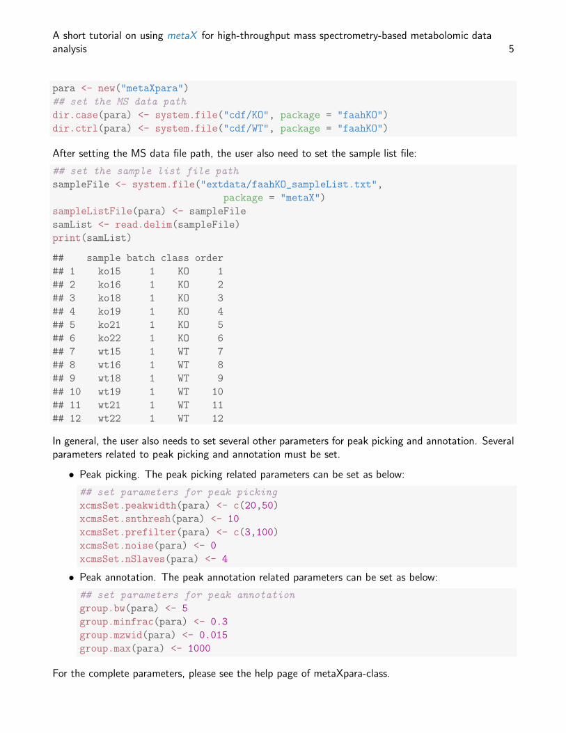
After setting the MS data file path, the user also need to set the sample list file:

## set the sample list file path

sampleFile <- system.file("extdata/faahKO_sampleList.txt",

package = "metaX")

sampleListFile(para) <- sampleFile

samList <- read.delim(sampleFile)

print(samList)

## sample batch class order

## 1 ko15 1 KO 1

## 2 ko16 1 KO 2

## 3 ko18 1 KO 3

## 4 ko19 1 KO 4

## 5 ko21 1 KO 5

## 6 ko22 1 KO 6

## 7 wt15 1 WT 7

## 8 wt16 1 WT 8

## 9 wt18 1 WT 9

## 10 wt19 1 WT 10

## 11 wt21 1 WT 11

## 12 wt22 1 WT 12

In general, the user also needs to set several other parameters for peak picking and annotation. Severalparameters related to peak picking and annotation must be set.

• Peak picking. The peak picking related parameters can be set as below:

## set parameters for peak picking

xcmsSet.peakwidth(para) <- c(20,50)

xcmsSet.snthresh(para) <- 10

xcmsSet.prefilter(para) <- c(3,100)

xcmsSet.noise(para) <- 0

xcmsSet.nSlaves(para) <- 4

• Peak annotation. The peak annotation related parameters can be set as below:

## set parameters for peak annotation

group.bw(para) <- 5

group.minfrac(para) <- 0.3

group.mzwid(para) <- 0.015

group.max(para) <- 1000

For the complete parameters, please see the help page of metaXpara-class.



In metaX , there is a function peakFinder(), which can be used to do the peak picking and annotation.

p <- peakFinder(para)

For the complete parameters, please see the help page of metaXpara-class.

3.2 Integrated function metaXpipe()

The function metaXpipe automates the whole data analysis process. In general, the user only need touse this function to do most of the analysis. It includes the following steps:

1. Peak picking and annotation when input MS data.2. Data pre-processing: Firstly, if an metabolite feature is detected in <50% of QC samples or

detected in <20% of experimental samples, it is removed from the rest data analysis.3. Missing value imputation.4. Removal of outliers (sample).5. Normalization.6. Feature filter according to the CV (30%) of features in QC sample. It only works when there are

QC samples.7. Univariate statistical analysis, such as t test, Mann-Whitney U test and ROC analysis.8. PCA (score plot, loading plot)9. PLS-DA (score plot, loading plot, permutation test, Q2, R2)

10. Assessment of data quality:(a) The peak number distribution(b) The number of missing value distribution(c) The boxplot of peak intensity(d) The total peak intensity distribution(e) The correlation heatmap of QC samples if available(f) Metabolite m/z (or mass) distribution(g) Plot of m/z versus retention time(h) PCA score or loading plot of all samples

A complete example to show how to run the integrated analysis is shown below:






ratioPairs(para) <- "S:C"

plsdaPara <- new("plsDAPara")

para@outdir <- "output"

p <- metaXpipe(para,plsdaPara=plsdaPara,cvFilter=0.3,remveOutlier = TRUE,

outTol = 1.2, doQA = TRUE, doROC = TRUE, qcsc = FALSE,

nor.method = "pqn", pclean = TRUE, t = 1, scale = "uv",)




In the above example, the class plsDAPara from metaX is used to control the parameters for PLS-DAanalysis. For the complete parameters, please see the help page of plsDAPara-class.

After the analysis has completed, the file ”index.html” in the output directory can be opened in a webbrowser to access report generated.

3.3 Function modules

3.3.1 Peak picking and annotation

In metaX, the function peakFinder() can be used to do the peak picking and annotation. It uses theXCMS to perform peak picking, followed by the CAMERA [4] package to perform peak annotation.

3.3.2 Missing value imputation

Missing value imputation. Missing values is a common phenomenon in a typical quantitative metabolomicsdataset. There are several methods provided by metaX to process the missing value. Currently, weimplemented a variety of methods which enable users to automatically perform missing value imputationby min, Probabilistic PCA (PPCA), Bayesian PCA (BPCA), k nearest-neighbor (KNN), missForest andSingular Value Decomposition Imputation (SVDImpute).

When the user uses the function metaXpipe to do the analysis, the following code can be used to setthe imputation method:

## bpca, svdImpute, knn, rf, min

missValueImputeMethod(para) <- "knn"

Also, the user can use the function missingValueImpute to perform the missing value imputation:






para <- reSetPeaksData(para)

## bpca, svdImpute, knn, rf, min

para <- missingValueImpute(para,method="knn")

## missingValueImpute: value

## Sun May 15 22:35:27 2016 Missing value imputation for ’value’

## Missing value in total: 3940

## Missing value in QC sample: 678

## Missing value in non-QC sample: 3262






QC QC QC S S S ... QC S S S ... QC QC QC

Sample injection order

Figure 1: The experiment design which contained QC samples.

## Sun May 15 22:35:27 2016 The ratio of missing value: 4.5814%

## <=0: 0

## Missing value in total after missing value inputation: 0

## <=0 value in total after missing value inputation: 0

3.3.3 Normalization

Currently, we implemented several methods to perform data normalization, such as the QC-robust splinebatch correction (QC-RSC) [5], sum, VSN, probabilistic quotient normalization (PQN) [6], quantilesand robust quantiles.

If there are pooled QC samples in the experiment (the experiment is like figure 1), the function doQCRLSC

can be used to perform the QC-RSC normalization. This method is implemented to correct data withinbatch experiment analytical variation, and batch-to-batch variation in large-scale studies.




rawPeaks(para) <- read.delim(pfile,check.names = FALSE)[1:100,]



para <- missingValueImpute(para)

res <- doQCRLSC(para,cpu=1)

Except the QC-RSC method, the user can use the other method (PQN, sum et al.) as below:










para <- metaX::normalize(para,method="pqn",valueID="value")

3.3.4 Pre-processing of raw peak data

In metaX , two functions, filterQCPeaks() and filterPeaks() can be used to filter features. Ingeneral, an metabolite feature is detected in <50% of QC samples (by using filterQCPeaks()) ordetected in <20% (by using filterPeaks()) of experimental samples, it is removed from the restdata analysis.







p <- filterPeaks(para,ratio=0.2)

p <- filterQCPeaks(para,ratio=0.5)

3.3.5 Removal of outliers

metaX provides function (RfunctionautoRemoveOutlier()) to automatically remove the outlier samplesin the pre-processed data based on expansion of the Hotellings T2 distribution ellipse. A sample withinthe first and second component PCA score plot beyond the expanded ellipse is removed, then the PCAmodel is recalculated. In default, three rounds of outlier removal are performed.








rs <- autoRemoveOutlier(para,valueID="value")

3.3.6 Power analysis and sample size estimation

In metaX , the function powerAnalyst() can be used to do power analysis and sample size estimation.



















## <=0: 0



para <- metaX::normalize(para)

## normalize: value

para <- transformation(para,valueID = "value")

para <- preProcess(para,scale = "pareto",valueID="value")

res <- powerAnalyst(para,group=c("C","S"),log=FALSE,

maxInd=200,showPlot = TRUE)

##

## C S

## 66 68

## .//metaX-power.pdf

print(res)

## [1] 0.7543686

3.3.7 Metabolite correlation network analysis

In metaX , the function plotNetwork() can be used to do correlation network analysis.







●

●

●

●

●

●

●

●

●

●

0.2

0.4

0.6

0.8

0 50 100 150 200Sample Size (per group)

Pre

dict

ed p

ower

Figure 2: The power and sample size distribution.











## <=0: 0



op <- par()

par(mar=c(0,0,0,0))

gg <- plotNetwork(para,group=c("S","C"),degree.thr = 10,



●

●

●

●●

●

●

●

●

●

●● ●

●

●

●

148.00249

149.00726

245.96823

408.02083

419.08758429.2632

443.23403

447.24411

454.04056

461.95596

462.88117

462.96682

468.88917

470.0144 471.06169

485.9441

495.06697

519.2953

Figure 3: The correlation network.

cor.thr = 0.85,showPlot=TRUE)

## V: 18

## E: 111

## .//metaX-network.pdf

par(op)



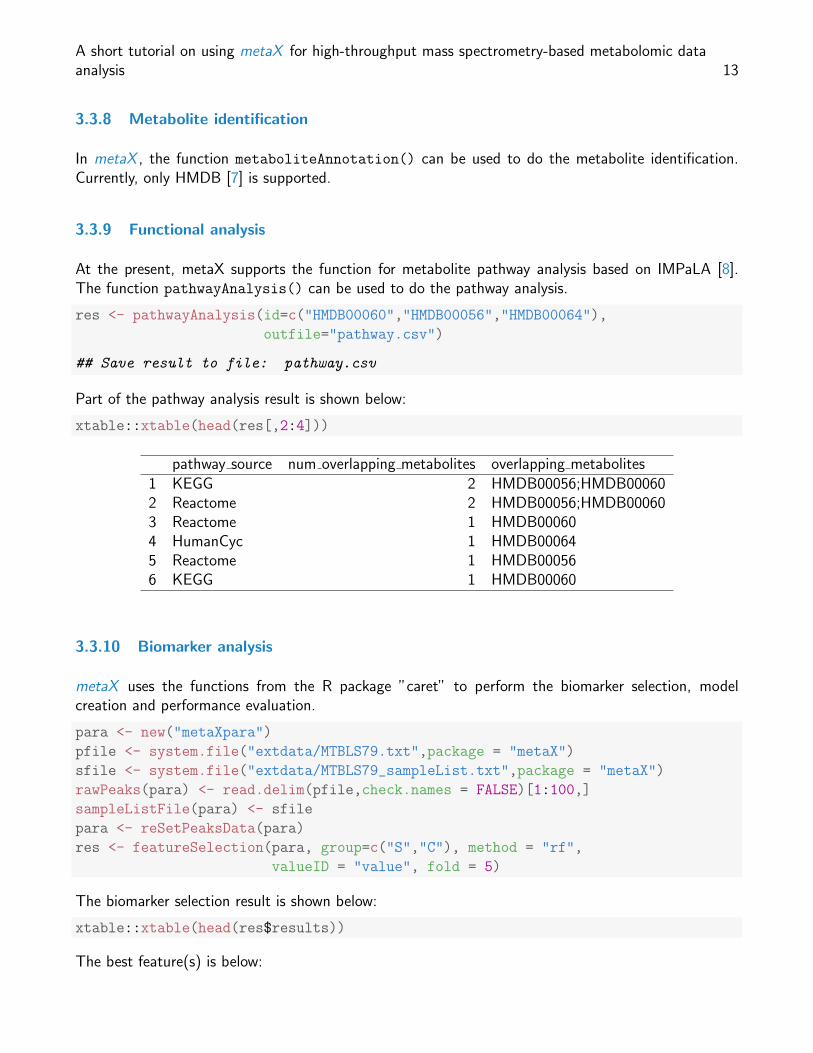
3.3.8 Metabolite identification

In metaX , the function metaboliteAnnotation() can be used to do the metabolite identification.Currently, only HMDB [7] is supported.

3.3.9 Functional analysis

At the present, metaX supports the function for metabolite pathway analysis based on IMPaLA [8].The function pathwayAnalysis() can be used to do the pathway analysis.

res <- pathwayAnalysis(id=c("HMDB00060","HMDB00056","HMDB00064"),

outfile="pathway.csv")

## Save result to file: pathway.csv

Part of the pathway analysis result is shown below:

xtable::xtable(head(res[,2:4]))

pathway source num overlapping metabolites overlapping metabolites1 KEGG 2 HMDB00056;HMDB000602 Reactome 2 HMDB00056;HMDB000603 Reactome 1 HMDB000604 HumanCyc 1 HMDB000645 Reactome 1 HMDB000566 KEGG 1 HMDB00060

3.3.10 Biomarker analysis

metaX uses the functions from the R package ”caret” to perform the biomarker selection, modelcreation and performance evaluation.







res <- featureSelection(para, group=c("S","C"), method = "rf",

valueID = "value", fold = 5)

The biomarker selection result is shown below:

xtable::xtable(head(res$results))

The best feature(s) is below:





Variables Accuracy Kappa AccuracySD KappaSD1 1.00 0.98 0.95 0.02 0.042 2.00 0.99 0.98 0.02 0.033 3.00 1.00 1.00 0.00 0.004 4.00 1.00 1.00 0.00 0.005 5.00 1.00 1.00 0.00 0.006 6.00 1.00 1.00 0.00 0.00

print(res$optVariables)

[1] ”461.95596” ”204.13419” ”295.04729”

3.3.11 Data transformation

There are two methods which can be used to do transformation, log transformation and cube roottransformation. The function transformation() can be used to do transformation like below:














## <=0: 0



para <- transformation(para,valueID = "value",method=1)



3.3.12 Data scaling

There are three methods which can be used to do scaling, ”pareto”, ”vector”, ”uv”. The functionpreProcess() can be used to do scaling like below:














## <=0: 0



para <- metaX::preProcess(para,valueID = "value",scale="uv")

3.3.13 Univariate statistical analysis

For univariate statistical analysis, the parametric statistical test (t test), non-parametric statistical test(Mann-Whitney U test), and classical univariate receiver operating characteristic (ROC) curve analysisare implemented. The function peakStat() can be used to do these analysis.








ratioPairs(para) <- "S:C"

addValueNorm(para) <- para


plsdaPara@nperm <- 10



res <- peakStat(para,plsdaPara,doROC = TRUE)

The part of the analysis result is shown below:

head(res@quant)

## ID ratio t.test_p.value wilcox.test_p.value t.test_p.value_BHcorrect

## 1 102.09132 1.0686877 4.474695e-01 5.643959e-01 5.736789e-01

## 2 133.06077 0.7184348 2.718336e-09 1.975226e-08 1.235607e-08

## 3 133.07219 1.0000180 9.179260e-01 7.135023e-01 9.179260e-01

## 4 136.0474 1.0632009 4.299989e-01 6.134752e-01 5.657880e-01

## 5 138.96337 0.8847494 1.941816e-03 3.882242e-05 4.623372e-03

## 6 144.10058 0.9765783 2.594286e-01 2.555067e-01 3.706123e-01

## wilcox.test_p.value_BHcorrect roc lowROC upROC VIP sample

## 1 6.882876e-01 0.4710339 0.3776181 0.5626337 0.19444924 S:C

## 2 7.597022e-08 0.7811943 0.6967357 0.8523173 1.41948421 S:C

## 3 7.927803e-01 0.5184938 0.4194352 0.6122995 0.02918377 S:C

## 4 7.303277e-01 0.4745989 0.3811107 0.5738525 0.19682177 S:C

## 5 1.021643e-04 0.7061052 0.6138369 0.7970254 0.75880701 S:C

## 6 3.650096e-01 0.5570410 0.4661514 0.6550858 0.33906390 S:C

3.3.14 PCA

The PCA analysis can be performed by the function plotPCA() in metaX . The score plot (as shownin figure 4) for 2D plot, figure 5) for 3D plot) and loading plot (as shown in figure 6)) are outputed.








para <- transformation(para,valueID = "value")

metaX::plotPCA(para,valueID="value",scale="pareto",center=TRUE,rmQC = FALSE)

## $fig

## [1] ".//metaX-PCA.png"

##

## $highfig

## [1] ".//metaX-PCA.pdf"

##

## $pca

## svdImpute calculated PCA

## Importance of component(s):




123

4

5

6

7

89

10

11

12

13

1415

1617

18

1920

2122

23

24

25 2627

28

29

30

3132

33

34

35

3637 38

3940

41

42 43

44 4546

47

48

495051

52

53

54

55

56

57

58

59

60

6162

6364

65

66

67

68

69

70

71

72

737475

76

7778

7980

81

82

83 84

85

86

87

88

8990

9192

93

94

9596

97

98

99100

101

102

103

104

105106

107

108

109

110

111

112

113114

115

116

117

118

119120

121

122

123

124

125

126

127

128

129

130

131

132133

134

135

136

137138

139

140

141

142

143144

145

146 147148

149

150

151

152153

154

155

156

157158

159160161

162

163 164

165

166

167

168

169

170

171

172

●●

●

●

●

●

●

●●

●

●

●

●

●

●

●

●

●

●

●

●

●

●

●

●●

●

●

●

●

●

●

●

●

●

●●

●

●●

●

● ●

●●●

●

●

●●

●

●

●

●

●

●

●

●

●

●

●

●

●●

●

●

●

●

●

●

●

●

●●

●

●

●

●

●●

●

●

●●

●

●

●

●

●

●

●●

●

●

●●

●

●

●●

●

●

●

●

●

●

●

●

●

●

●

●

●●

●

●

●

●

●

●

●

●

●

●

●

●

●

●

●

●

●

●●

●

●

●

●

●

●

●

●

●

●●

●

●●

●

●

●

●

●

●

●

●

●

●

●

●●●

●

●●

●

●

●

●

●

●

●

●

−20

−10

0

10

−10 0 10PC1 (23.36%)

PC

2 (1

5.44

%)

class a● a● a●C QC S

Figure 4: The PCA score plot.

## PC1 PC2 PC3

## R2 0.2336 0.1544 0.1026

## Cumulative R2 0.2336 0.3880 0.4905

## 500 Variables

## 172 Samples

## 0 NAs ( 0 %)

## 3 Calculated component(s)

## Data was mean centered before running PCA

## Data was scaled before running PCA

## Scores structure:

## [1] 172 3

## Loadings structure:

## [1] 500 3



−15 −10 −5 0 5 10 15−15

−10

−5

0 5

10

−15−10

−5 0

5 10

15

PC1 (23.36%)

PC

2 (1

5.44

%)

PC

3 (1

0.26

%)

●●●

●

●●

●

●

●●

●

●

●

●●

●

●

●

●●

●●

●

●

●●

●

●

●

●●

●● ●

●

●●

●

●●

●

●

●●●

●

●

●

●

●

●

●

●

●

●

●

●

●

●

●

●

●

●●

●

●●

● ●●

●

●

●●

●

●

●●●●

●

●

●

●

●

●

●

●●

●

●●

●

●●

●

●

●

●●

●

●●

●

● ●

●

●

●

●●

●

●

●●

●

●

●

●

●

●

●

●

●

●

●●

●

●

●

●●

●

●

●

●

●● ●

●

● ● ●

●

●

● ●

●●

●

●

●

●

●

●

●

●

●

●●●

●

●●

●

●

●●●

●

●

●

123

4

56

7

8

910

11

12

13

1415

16

17

18

1920

2122

23

24

2526

27

28

29

3031

3233 34

35

3637

38

3940

41

42

434445

46

47

48

49

50

51

52

53

54

55

56

57

58

59

60

61

62

6364

65

6667

68 6970

71

72

7374

75

76

77787980

81

82

83

84

85

86

87

8889

90

9192

93

9495

96

97

98

99100

101

102103

104

105 106

107

108

109

110111

112

113

114115

116

117

118

119

120

121

122

123

124

125

126127

128

129

130

131132

133

134

135

136

137138 139

140

141 142143

144

145

146 147

148149

150

151

152

153

154

155

156

157

158

159160161

162

163164

165

166

167168169

170

171

172

●

●

●

CQCS

Figure 5: The 3D PCA score plot.

3.3.15 PLS-DA

The PLS-DA analysis can be performed by the function runPLSDA() in metaX . The R2, Q2 and thepermutation test p-value are calculated and outputed. The permutation test plot is shown in figure 7.The score plot and loading plot are shown in figure 8 and figure 9, respectively.








para <- metaX::normalize(para,method="pqn")


plsdaPara@nperm <- 100

plsda.res <- runPLSDA(para = para,plsdaPara = plsdaPara,




112.0523

148.00249

148.00448

149.00726

176.00503

187.62759189.01599

190.11863

245.96823

279.19144

282.01283

283.01892

295.04729

303.24558

305.97518

306.21938316.20023320.2175320.22895

321.24607323.24496324.24879

334.26767

342.31152

346.25071

348.26637369.32242

370.19102

370.31458371.3268372.24546

373.2446374.24796

375.20702

381.07937

382.28018

386.21715399.33298

404.03555

408.02083

413.34863

414.33272

416.27477

416.30205

419.08758

419.32428

429.2632

437.34873

443.06252

443.23403447.24411

448.31465

451.30499

451.33351452.19103

454.04056

454.15227

456.29327

456.32956

458.01805461.95596

462.88117462.96682

466.30425

468.88917

470.0144471.06169

473.08515

474.32861

478.24156

479.33596

483.20561

485.9441

495.0546

495.06697

519.2953

545.50201

548.99712

557.48449

557.49077

−0.10

−0.05

0.00

0.05

0.10

−0.10 −0.05 0.00 0.05 0.10PC1

PC

2

Figure 6: The PCA loading plot.

sample = c("S","C"),valueID="value")

cat("R2Y: ",plsda.res$plsda$res$R2,"\n")

## R2Y: 0.9847925

cat("Q2Y: ",plsda.res$plsda$res$Q2,"\n")

## Q2Y: 0.9803359

## permutation test

cat("P-value R2Y: ",plsda.res$pvalue$R2,"\n")

## P-value R2Y: 0

cat("P-value Q2Y: ",plsda.res$pvalue$Q2,"\n")

## P-value Q2Y: 0



●●

●

●●●●●

●●●●●

●

●

●

●

●

●●

●

●●●●

●●

●

●

●

●●●●●

●

●●●●●

●●

●●●●●

●●●●

●●●

●

●●

●●●

●●●●●●●●●

●●●

●

●●●

●

●

●●●

●

●●

●●

●

●●●

●●

●●●●●

●●

●

0.0 0.2 0.4 0.6 0.8 1.0

−0.

50.

00.

51.

0

Cor

Val

ue

● R2Q2

Intercepts: R2=(0.0, 0.1952 ), Q2=(0.0, −0.3191 )

Figure 7: The permutation test plot for PLS-DA.

3.3.16 Assessment of data quality

In metaXpipe, pre- and post-normalization, the data quality is visually assessed in several aspects:

1. The peak number distribution2. The number of missing value distribution3. The boxplot of peak intensity4. The total peak intensity distribution5. The correlation heatmap of QC samples if available6. The metabolite m/z (or mass) distribution7. The plot of m/z versus retention time8. The PCA score or loading plot of all samples (only available for post-normalization).

The example figures can be viewed in website http://wenbostar.github.io/metaX/.


http://wenbostar.github.io/metaX/


●

●

●

●

●

●

●

●

●

●

●

●

●

●

●●●

●●

●

●

●

●

●

●

●●

●

●

●

●

●

●●

●●

●

●

●

●

●

●

●

●

●

●●

●

●

●

●

●

●●

●

●

●

●

●

●

●

●

●

●

●

●

●

●●

●

●

●

●

●

●

●

●

●

●

●

●

●

●

●

●

●

●

●

●●

●● ●

●

●

●

●

●

●

●

● ●

●

●

●

●

●

●

●

●

●

●

●

●

●●

●

●

●

●

●

●●

●

●

●

●

●

●

●

●

●

●

●

4

5

6

8

9

1011

12

1415

16

17

19

20

212224

25 26

27

28

30

31

32

33

3436

37

38

3940

42

4344

454648

49

50

51

52

54

55

56

57

586061

62

6364

66

6768

6970

7273

74

7577

78

79

80

82

83

84

8586

8889

90

93

94

95

96

98

99

100

102

103

105

106

107

110

111

113

114

115116

117119 120

121

122

124

125

126127

130

131132

133

134

136

137

138

139141

142

143

144

146

147

148149151

152

153

154

155

157158

159

160

161163

164

165

167

168169

170171

−10

−5

0

5

10

−10 0 10PC1 (25.11%)

PC

2 (5

.75%

)

class●a●a

C

S

Figure 8: The score plot for PLS-DA.

4 Frequently asked questions

4.1 How to select the best number of components for PLS-DA?

The function selectBestComponent can be used to select the best number of components for PLS-DA.This function calculates the R2 and Q2 for each component.








para <- metaX::normalize(para,method="pqn",valueID="value")

selectBestComponent(para,np=10,sample=c("S","C"),scale="pareto",valueID="value",k=5)



123.05466

143.04851

151.04693

167.02004

167.02071

170.06172

203.05255

207.01269

207.01423

222.98638

245.95415

261.20022

311.031

335.98592

369.05739

370.05237

371.0557

387.02378394.21591

403.05166

416.14128

416.30205

423.98216

425.02104

447.17138452.04444

454.09714

462.98951

468.88917

470.9348

474.00137

477.09659

−0.1

0.0

0.1

−0.10 −0.05 0.00 0.05 0.10PC1

PC

2

Figure 9: The loading plot for PLS-DA.

4.2 How to set the comparison groups?

We can use the following method to set the comparison groups:

ratioPairs(para) <- "KO:WT"

If multiple comparison groups must be set in a single analysis, the user can set the ”para@ratioPairs”like ”A:B;C:B;D:B”, each comparison group is separated by semicolon.

ratioPairs(para) <- "A:B;C:B;D:B"

4.3 How to set the output file directory?

The user can set the output directory and the prefix of the output files as below:

## set the output parameters

outdir(para) <- "test"



prefix(para) <- "metaX"

Session information

All software and respective versions used to produce this document are listed below.

• R version 3.3.0 (2016-05-03), x86_64-pc-linux-gnu• Locale: LC_CTYPE=en_US.UTF-8, LC_NUMERIC=C, LC_TIME=en_US.UTF-8, LC_COLLATE=C,LC_MONETARY=en_US.UTF-8, LC_MESSAGES=en_US.UTF-8, LC_PAPER=en_US.UTF-8,LC_NAME=C, LC_ADDRESS=C, LC_TELEPHONE=C, LC_MEASUREMENT=en_US.UTF-8,LC_IDENTIFICATION=C

• Base packages: base, datasets, grDevices, graphics, grid, methods, parallel, stats, utils• Other packages: Biobase 2.32.0, BiocGenerics 0.18.0, ProtGenerics 1.4.0, Rcpp 0.12.5,

SSPA 2.12.0, VennDiagram 1.6.17, caret 6.0-68, data.table 1.9.6, dplyr 0.4.3, futile.logger 1.4.1,ggplot2 2.1.0, lattice 0.20-33, limma 3.28.4, metaX 1.4.2, mzR 2.6.2, pROC 1.8, pls 2.5-0,plyr 1.8.3, qvalue 2.4.2, randomForest 4.6-12, reshape2 1.4.1, scatterplot3d 0.3-36, xcms 1.48.0• Loaded via a namespace (and not attached): BBmisc 1.9, BiocInstaller 1.22.2, BiocStyle 2.0.2,

CAMERA 1.28.0, DBI 0.4-1, DiffCorr 0.4.1, DiscriMiner 0.1-29, Formula 1.2-1, Hmisc 3.17-4,MASS 7.3-45, Matrix 1.2-6, MatrixModels 0.4-1, Nozzle.R1 1.1-1, R6 2.1.2, RBGL 1.48.0,RColorBrewer 1.1-2, RCurl 1.95-4.8, SparseM 1.7, acepack 1.3-3.3, affy 1.50.0, affyio 1.42.0,ape 3.4, assertthat 0.1, backports 1.0.2, bitops 1.0-6, boot 1.3-18, bootstrap 2015.2, car 2.1-2,checkmate 1.7.4, chron 2.3-47, class 7.3-14, cluster 2.0.4, codetools 0.2-14, colorspace 1.2-6,compiler 3.3.0, corpcor 1.6.8, digest 0.6.9, doParallel 1.0.10, e1071 1.6-7, ellipse 0.3-8,evaluate 0.9, faahKO 1.12.0, fdrtool 1.2.15, foreach 1.4.3, foreign 0.8-66, formatR 1.4,futile.options 1.0.0, graph 1.50.0, gridExtra 2.2.1, gtable 0.2.0, highr 0.6, igraph 1.0.1,impute 1.46.0, iterators 1.0.8, itertools 0.1-3, knitr 1.13, labeling 0.3, lambda.r 1.1.7,latticeExtra 0.6-28, lazyeval 0.1.10, lme4 1.1-12, magrittr 1.5, mgcv 1.8-12, minqa 1.2.4,missForest 1.4, mixOmics 5.2.0, multtest 2.28.0, munsell 0.4.3, nlme 3.1-128, nloptr 1.0.4,nnet 7.3-12, pbkrtest 0.4-6, pcaMethods 1.64.0, pheatmap 1.0.8, preprocessCore 1.34.0,quantreg 5.24, rgl 0.95.1441, rpart 4.1-10, scales 0.4.0, splines 3.3.0, stats4 3.3.0, stringi 1.0-1,stringr 1.0.0, survival 2.39-4, tidyr 0.4.1, tools 3.3.0, vsn 3.40.0, xtable 1.8-2, zlibbioc 1.18.0

References

[1] Alan Saghatelian, Sunia A Trauger, Elizabeth J Want, Edward G Hawkins, Gary Siuzdak, andBenjamin F Cravatt. Assignment of endogenous substrates to enzymes by global metabolite profiling.Biochemistry, 43(45):14332–14339, 2004.

[2] Jennifer A Kirwan, Ralf JM Weber, David I Broadhurst, and Mark R Viant. Direct infusion massspectrometry metabolomics dataset: a benchmark for data processing and quality control. Scientificdata, 1, 2014.



[3] Mikko Katajamaa, Jarkko Miettinen, and Matej Oresic. Mzmine: toolbox for processing and visu-alization of mass spectrometry based molecular profile data. Bioinformatics, 22(5):634–636, 2006.

[4] Carsten Kuhl, Ralf Tautenhahn, Christoph Bttcher, Tony R Larson, and Steffen Neumann. Camera:an integrated strategy for compound spectra extraction and annotation of liquid chromatogra-phy/mass spectrometry data sets. Analytical chemistry, 84(1):283–289, 2011.

[5] Warwick B Dunn, David Broadhurst, Paul Begley, Eva Zelena, Sue Francis-McIntyre, Nadine An-derson, Marie Brown, Joshau D Knowles, Antony Halsall, John N Haselden, et al. Proceduresfor large-scale metabolic profiling of serum and plasma using gas chromatography and liquid chro-matography coupled to mass spectrometry. Nature protocols, 6(7):1060–1083, 2011.

[6] Frank Dieterle, Alfred Ross, Gotz Schlotterbeck, and Hans Senn. Probabilistic quotient normaliza-tion as robust method to account for dilution of complex biological mixtures. application in 1h nmrmetabonomics. Analytical chemistry, 78(13):4281–4290, 2006.

[7] David S Wishart, Timothy Jewison, An Chi Guo, Michael Wilson, Craig Knox, Yifeng Liu, YannickDjoumbou, Rupasri Mandal, Farid Aziat, Edison Dong, et al. Hmdb 3.0the human metabolomedatabase in 2013. Nucleic acids research, page gks1065, 2012.

[8] Atanas Kamburov, Rachel Cavill, Timothy MD Ebbels, Ralf Herwig, and Hector C Keun. Inte-grated pathway-level analysis of transcriptomics and metabolomics data with impala. Bioinformatics,27(20):2917–2918, 2011.


a short tutorial on using metax for high-throughput mass...

Documents