a simple estimator for the distribution of random coefficients
TRANSCRIPT

Quantitative Economics 2 (2011), 381–418 1759-7331/20110381
A simple estimator for the distribution of random coefficients
Jeremy T. FoxUniversity of Michigan and NBER
Kyoo il KimUniversity of Minnesota
Stephen P. RyanMIT and NBER
Patrick BajariUniversity of Minnesota and NBER
We propose a simple mixtures estimator for recovering the joint distribution ofparameter heterogeneity in economic models, such as the random coefficientslogit. The estimator is based on linear regression subject to linear inequality con-straints, and is robust, easy to program, and computationally attractive comparedto alternative estimators for random coefficient models. For complex structuralmodels, one does not need to nest a solution to the economic model during op-timization. We present a Monte Carlo study and an empirical application to dy-namic programming discrete choice with a serially correlated unobserved statevariable.Keywords. Random coefficients, mixtures, demand, logit, mixed logit, dynamicprogramming, teacher labor supply.
JEL classification. C25, C14, L.
1. Introduction
In economics, it is common to observe that otherwise identical agents behave differ-ently when faced with identical choice environments, due to such factors as hetero-
Jeremy T. Fox: [email protected] il Kim: [email protected] P. Ryan: [email protected] Bajari: [email protected] thanks the National Science Foundation, the Olin Foundation, and the Stigler Center for generousfunding. Bajari thanks the National Science Foundation, Grant SES-0720463, for generous research sup-port. Thanks to helpful comments from seminar participants at the AEA meetings, Chicago, Chicago GSB,UC Davis, European Commission Antitrust, the Far East Econometric Society meetings, LSE, Mannheim,MIT, Northwestern, Paris I, Quantitative Marketing and Economics, Queens, Rochester, Rutgers, Stanford,Stony Brook, Toronto, UCL, USC, UT Dallas, Virginia, and Yale. Thanks to comments from Xiaohong Chen,Andrew Chesher, Philippe Fevrier, Amit Gandhi, Han Hong, David Margolis, Andrés Musalem, Peter Reiss,Jean-Marc Robin, Andrés Santos, Azeem Shaikh, and Harald Uhlig. Thanks to Chenchuan Li for researchassistance.
Copyright © 2011 Jeremy T. Fox, Kyoo il Kim, Stephen P. Ryan, and Patrick Bajari. Licensed under theCreative Commons Attribution-NonCommercial License 3.0. Available at http://www.qeconomics.org.DOI: 10.3982/QE49

382 Fox, Kim, Ryan, and Bajari Quantitative Economics 2 (2011)
geneity in preferences. A classic example is that consumers may have heterogeneouspreferences over a set of product characteristics in an industry with differentiated prod-ucts. A growing econometric literature has addressed heterogeneity by providing esti-mators that allow the coefficients of the economic model to vary across agents. In thispaper, we describe a general method for estimating such random coefficient modelsthat is easy to compute. Our estimator exploits a reparametrization of the underlyingmodel so that the parameters enter linearly. This is in contrast to previous approachesin the literature, such as the expectation-maximization (EM) algorithm, Markov chainMonte Carlo (MCMC), simulated maximum likelihood, simulated method of moments,and minimum distance, which are highly nonlinear. Linearity simplifies the computa-tion of the parameters. Our approach also avoids nested solutions to economic modelsin optimization, which gives a strong computational advantage for complex structuralmodels, as we will discuss.
To motivate our approach, consider the following simple example. Suppose that theeconometrician is interested in estimating a binary logit model with a scalar randomcoefficient. Let y = 1 if the first option is chosen and let y = 0 otherwise. Suppose thatthis model has a single independent variable, x. Furthermore, suppose that the randomcoefficient is known to have support on the [0�1] interval. Fix a large but finite grid of Requally spaced points. Suppose that the grid points take on the values 1
R�2R� � � � �
R−1R �1.
The parameters of our model are θr , the frequencies of each random coefficient rR . It
then follows that the empirical probability that the dependent variable y is 1 conditionalon x can be approximated by the linear combination
Pr(y = 1 | x)≈R∑r=1
θrexp
(r
R· x
)
1 + exp(r
R· x
) �
The key insight of our approach is that the dependent variable in our model, Pr(y = 1 |x), is linearly related to the model parameters θr , irrespective of the nonlinear modelused to compute the probability under a given type r. Instead of optimizing over thatnonlinear model, we compute the probability under each type as if it were the true pa-rameter, and then find the proper mixture of those models that best approximates theactual data. We demonstrate that the θr parameters can be consistently estimated us-ing inequality constrained least squares. This estimator has a single global optimum,and widely available specialized minimization approaches are guaranteed to convergeto that point. This contrasts with alternative approaches to estimating random coef-ficient models, where the objective functions can have multiple local optima and theeconometrician is not guaranteed to find the global solution.
Many alternative estimators require computationally expensive nonlinear optimiza-tion, and as a result researchers frequently use tightly specified distributions of hetero-geneity in applied work because of computational constraints. For example, applied re-searchers frequently assume that the random coefficients are mutually independent andnormal. Our approach allows us to estimate the joint distribution of random coefficientswithout having to impose a parsimonious family of distributions.

Quantitative Economics 2 (2011) Distribution of random coefficients 383
We show how to extend this simple intuition to a more general framework. Model-ing the random coefficients using equally spaced grid points does not lead to a smoothestimated density. We suggest alternative methods for discretizing the model that givesmooth densities, while still maintaining the linear relationship between the dependentvariable and the model parameters. Also, we extend our approach to accommodate thecase where the support of the basis functions is not known, and the econometricianmust search over the location and the scale of the parameter space. Further, we intro-duce a cross-validation method for picking the grid points.
Importantly, we discuss how our approach can be extended to more complex, struc-tural economic choice models. As an example, we show how to estimate a distributionof random coefficients in a dynamic programming, discrete choice model such as Rust(1987). The computational issues in traditional simulation estimators applied to staticmodels are more severe for dynamic models when the dynamic programming problemmust be solved for each realization of the random coefficients in each call of the ob-jective function by the optimization routine. If there are S simulation draws in a tradi-tional simulation estimator and the optimization routine requires L evaluations of theobjective function to achieve convergence, the dynamic programming problem mustbe solved S ·L times in the traditional approach. In our estimator, the dynamic programmust be solved only R times, when R is the number of support points for the randomcoefficients. In our dynamic programming empirical application to teacher labor supplyin India, we demonstrate that our approach can dramatically reduce the computationalburden of these models.
Our estimator is a general mixtures estimator. A frequent application of mixtures es-timators in the literature has been demand estimation. In the paper, we discuss somestrengths and weaknesses of our approach relative to some other approaches proposedin the demand estimation literature. First, if the researcher has aggregate data on mar-ket shares with price endogeneity, the approach of Berry, Levinsohn, and Pakes (1995)will impose fewer assumptions on the supply side of the model. Our approach can ac-commodate aggregate data, even if market shares are measured with error, which Berryet al. do not allow. However, we need to specify a reduced-form pricing function anal-ogous to the pricing functions in Kim and Petrin (2010) and especially Fox and Gandhi(2010) in order to account for price endogeneity (or adapt the arguments in Berry andHaile (2010b) and Fox and Gandhi (2011b)). It is not possible to prove the existence ofthe particular pricing function that we use from general supply-side assumptions. Sec-ond, in small samples, Bayesian methods such as Rossi, Allenby, and McCulloch (2005)and Burda, Harding, and Hausman (2008) that use prior information will likely have bet-ter finite-sample performance, at the computational expense of having to evaluate theobjective function many times. Our methods are intended for applications where theresearcher has access to large sample sizes.
The most common frequentist, mixtures estimator is nonparametric maximum like-lihood or (NPMLE) (Laird (1978), Böhning (1982), Lindsay (1983), Heckman and Singer(1984)). Often the EM algorithm is used for computation (Dempster, Laird, and Rubin(1977)), but this approach is not guaranteed to find the global maximum. The litera-ture worries about the strong dependence of the output of the EM algorithm on initial

384 Fox, Kim, Ryan, and Bajari Quantitative Economics 2 (2011)
starting values as well as the difficulty in diagnosing convergence (Seidel, Mosler, andAlker (2000), Verbeek, Vlassis, and Kröse (2003), Biernacki, Celeux, and Govaert (2003),Karlis and Xekalaki (2003)).1 Further, the EM algorithm has a slow rate of convergenceeven when it does converge to a global solution (Pilla and Lindsay (2001)). Li and Bar-ron (2000) introduced another alternative, but again our approach is computationallysimpler. Our estimator is also computationally simpler than the minimum distance es-timator of Beran and Millar (1994), which in our experience often has an objective func-tion with an intractably large number of local minima. The discrete-grid idea (called thehistogram approach) is found outside of economics in Kamakura (1991), who used adiscrete grid to estimate an ideal-point model; he did not discuss any of our extensions.Of course, mixtures themselves have a long history in economics, such as Quandt andRamsey (1978).
The outline of our paper is as follows. In Section 2, we describe our model and base-line estimator. We focus on the motivating example of the multinomial logit with in-dividual data. Section 3 discusses picking the grid of points and introduces our cross-validation approach. Section 4 provides various extensions to the baseline estimator.Section 5 provides examples of discrete choice with aggregate data, dynamic program-ming discrete choice, mixed continuous and discrete choice (selection), and discretechoice models with endogenous regressors. We include a large number of examples soas to motivate our estimator for applied readers. In Section 6, we discuss how to con-duct inference. In Section 7, we conduct a Monte Carlo experiment to investigate thefinite-sample performance of our estimator. In Section 8, we apply our estimator to adynamic programming, discrete choice empirical problem studied in Duflo, Hanna, andRyan (forthcoming). The dynamic programming problem has a serially correlated, un-observed state variable.
2. The baseline estimator
2.1 General notation
We first introduce general notation. The econometrician observes a real-valued vectorof covariates x. The dependent variable in our model is denoted y and indicates an un-derlying random variable y∗ that takes values in the range of y∗, Y ∗. Note that y∗ is nota latent variable. In our examples, we focus primarily on the case where the range of y∗is a finite number of integer values as is customary in discrete choice models. However,much of our analysis extends to the case where y∗ is real-valued.
LetA denote a (measurable) set in the range of y∗, Y ∗. We let PA(x) denote the prob-ability that y∗ ∈A when the decision problem has characteristics x. Let β denote a ran-dom coefficient that we assume is distributed independently of x. In our framework, thisis a finite-dimensional, real-valued vector. We let gA(x�β) be the probability ofA condi-tional on the random coefficientsβ and characteristics x. The function gA is specified as
1Another drawback of NPMLE that is specific to mixtures of normal distributions, a common approxi-mating choice, is that the likelihood is unbounded and hence maximizing the likelihood does not producea consistent estimator. There is a consistent root but it is not the global maximum of the likelihood function(McLachlan and Peel (2000)).

Quantitative Economics 2 (2011) Distribution of random coefficients 385
a modeling primitive. In our simple example in the Introduction, gA corresponds to thelogit choice probability for a given coefficient β. The cumulative distribution function(CDF) of the random coefficients is denoted as F(β). We restrict our discussion of con-sistency and asymptotic inference to models with a finite number R of support pointsβr . The weight on the support point βr is θr ≥ 0, where
∑Rr=1 θr = 1. Given these defini-
tions, it follows that
PA(x)=R∑r=1
θrgA(x�βr)� (1)
On the right hand side of the above equation, gA(x�β) gives the probability of A con-ditional on x and β. We average over the distribution of β using the CDF F(β) =∑Rr=1 θ
r1[βr ≤ β], where 1[βr ≤ β] = 1 when βr ≤ β, to arrive at PA(x), the populationprobability of the eventA conditional on x.
In our framework, the object the econometrician wishes to estimate is the tuple(θ1� � � � � θR), the weights on the support points. For this paper, we assume the supportpoints are known (or known up to location and scale parameters in Section 4.3) andfocus on the computational advantages of our approach.
2.2 The multinomial logit model
As we discussed in the Introduction, one motivating example for our paper is the logitwith random coefficients. We begin by discussing this example in detail. In Section 5, weshow how our approach extends to other random coefficient models, including dynamicprogramming discrete choice and demand models where the dependent variable is rep-resented by a vector of discrete and continuous variables. The estimation method thatwe propose can, in principle, be applied to any model that can be written in the form(1). Indeed, in discrete choice with large samples, we can completely do away with thelogit errors and allow the distribution of the choice- and consumer-specific shocks to beestimated, which is a special case of the identification results on multinomial choice inFox and Gandhi (2010). Our examples start with the logit structure only for expositionalclarity, in part because the logit is commonly used in empirical work.
In the logit model, agents i= 1� � � � �N can choose between j = 1� � � � � J mutually ex-clusive alternatives and one outside good (good 0). The exogenous variables for choice jare in the K × 1 vector xi�j . In the example of demand estimation, xi�j might include thenonprice product characteristics, the price of good j, and the demographics of agent i.We let xi = (x′
i�1� � � � � x′i�J) denote the stacked vector of the J xi�j ’s, the observable charac-
teristics.In the model, there are r = 1� � � � �R types of agents. The unobservable preference
parameters of type r are equal to theK×1 vectorβr . We discuss how to choose the typesβr below. For the moment, assume that the βr are fixed and exogenously specified. Asin our example in the Introduction, it might be helpful to think of the βr being definedusing a fixed grid on a compact set. The random variable β is distributed independently

386 Fox, Kim, Ryan, and Bajari Quantitative Economics 2 (2011)
of x. The probability of type r in the population is θr . Let θ = (θ1� � � � � θR)′ denote thecorresponding vector. The θmust lie on the unit simplex, or
R∑r=1
θr = 1� (2)
θr ≥ 0� (3)
If agent i is of type r, her utility for choosing good j is equal to
ui�j = x′i�jβ
r + εi�j�There is an outside good with utility ui�0 = εi�0. Assume that εi�j is distributed as Type Iextreme value and is independent of xi and βr . Agents in the model are assumed to beutility maximizers. The observable dependent variable yi�j is generated as
yi�j ={
1� if ui�j > ui�j′ for all j′ �= j,0� otherwise.
Let yi be the vector (yi�1� � � � � yi�J). The probability of type r picking choice j at xi is (usingA= {j} in the general notation above)
gj(xi�βr)=
exp(x′i�jβ
r)
1 +J∑j′=1
exp(x′i�j′β
r)
�
It then follows that the conditional probability of observing that agent i selects choice jis
Pr(yi�j = 1 | xi)=R∑r=1
θrgj(xi�βr)=
R∑r=1
θrexp(x′
i�jβr)
1 +J∑j′=1
exp(x′i�j′β
r)
� (4)
2.3 Linear regression
We study the estimation problem of recovering θ given the researcher has i = 1� � � � �Nobservations on (xi� yi). A simple method for estimating the parameters θ is by ordinaryleast squares. To construct the estimator, begin by adding yi�j to both sides of (4) andmoving Pr(yi�j = 1 | xi) to the right side of this equation, which gives
yi�j =(
R∑r=1
θrgj(xi�βr)
)+ (yi�j − Pr(yi�j = 1 | xi)
)�
Define theR×1 vector zi�j = (zi�j�1� � � � � zi�j�R)′ with individual elements zi�j�r = gj(xi�βr).Recall that βr is fixed and is not a parameter to be estimated. As a result, given xi, theterm zi�j�r is a fixed regressor. Next, by the definition of a choice probability,
E[yi�j − Pr(yi�j = 1 | xi) | xi
] = 0� (5)

Quantitative Economics 2 (2011) Distribution of random coefficients 387
This implies that the following ordinary least-squares problem produces a consistentestimator of the θr :
θ= arg minθ
1NJ
N∑i=1
J∑j=1
(yi�j − z′i�jθ)
2�
LetY denote theNJ×1 vector formed by stacking the yi�j and letZ be theNJ×Rmatrixformed by stacking the zi�j . Then our estimator is θ= (Z′Z)−1Z′Y .
Equation (5) implies that the standard mean independence condition is satisfied forleast squares. The least-squares estimator has a unique solution as long asZ has rankR.The estimator is consistent under standard assumptions for least squares.
2.4 Inequality constrained linear least squares
A limitation of the ordinary least-squares estimator is that θ need not satisfy (2) and(3). In practice, one might wish to constrain θ to be a well defined probability measure.This would be useful in making sure that our model predicts probabilities that alwayslie between 0 and 1. Also, this may be important if the economist wishes to interpretthe distribution of β as a structural parameter. Our baseline estimator estimates θ usinginequality constrained least squares,
θ= arg minθ
1NJ
N∑i=1
J∑j=1
(yi�j − z′i�jθ)
2
(6)subject to (2) and (3)�
This minimization problem is a quadratic programming problem subject to linear in-equality constraints. The minimization problem is convex and routines like MATLAB’slsqlin guarantee finding a global optimum. One can construct the estimated cumulativedistribution function for the random coefficients as
FN(β)=R∑r=1
θr1[βr ≤ β]�
where 1[βr ≤ β] = 1 when βr ≤ β. Thus, we have a structural estimator for a distribu-tion of random parameters in addition to a method for approximating choice probabil-ities. We call the inequality-constrained least-squares estimator our baseline estimatorto distinguish it from several extensions below. This baseline estimator is consistent un-der standard regularity conditions (see, e.g., Newey and McFadden (1994) and Andrews(2002)).2
2Linear inequality constraints restrict only the parameter space of θ. Whether the estimator θ is on aboundary or is in the interior of the parameter space does not create any complications for establishingconsistency (Andrews (2002)). Standard sufficient conditions for the consistency of extremum estimatorsthat include our estimators are available in the literature.

388 Fox, Kim, Ryan, and Bajari Quantitative Economics 2 (2011)
3. Picking the grid of basis points
The approach just presented is computationally simple: we can always find a global op-timum and we avoid many evaluations of complex structural models, as we discuss inSection 5.1. The main disadvantage of the baseline approach is that the estimates maybe sensitive to the choice of the grid of points BR = (β1� � � � �βR). A natural first questionto ask about the baseline estimator is how to pick the number of grid pointsR as a func-tion of the sample. While our consistency arguments in this paper apply to a fixed R, inpractice we still need to choose R. Conditional on picking R, how should one pick theexact grid of points BR? This section addresses these questions. First we present advicebased on our experiences using the estimator in Monte Carlo experiments. Second, weadopt a data-driven cross-validation approach. In addition, Section 4.3 introduces analternative to cross-validation: a location and scale model for when the support of therandom coefficients is not known. We focus on the baseline estimator here.
3.1 Advice from Monte Carlos
We have run many Monte Carlo studies in the process of developing our estimator. InMonte Carlo experiments in Section 7, we set R = Cdim(xj) with dim(xj) = 2 for someconstants C. Although we find that typically more of the R weights are estimated to benonzero when the true F looks, roughly speaking, to be more complicated, our MonteCarlo experiments show that a relatively smallR can give a good approximation to F(β),whenN is large.
A drawback of the baseline estimator is that the researcher has to have some senseof the support of the random coefficients. In the logit, the econometrician may use apreliminary estimate of a logit model with fixed coefficients to determine a region ofsupport for the random coefficients. For example, the econometrician may center thegrid for the βr at the initial logit estimates and take some multiple of their confidenceintervals as the support or he or she can let the support for estimation grow as the sam-ple size grows.
A second, related approach to picking a support is that the econometrician may ex-periment with alternative sets of grid points to see how the choice of grid points in-fluences estimation results. A limitation of this approach is that it introduces a pretestbias and the standard errors in Section 6 will need to be adjusted. For example, a pro-cedure where a researcher uses a diffuse grid with a wide support and then reestimatesthe model after increasing the detail of the grid where mass appears to be located, is,in its full statistical structure, a two-step estimator. Rigorous standard errors should ac-count for both of the estimation steps. This approach is, however, acceptable when a re-searcher focuses on the approximation of the random coefficients distribution but notits inference.
Given a choice of support, we experimented with Halton and Weyl sequences; theytend to improve Monte Carlo performance over evenly spaced grids. We report in Sec-tion 7 that random grids did not work as well as evenly spaced grids in our investigations.

Quantitative Economics 2 (2011) Distribution of random coefficients 389
3.2 Cross-validation
Cross-validation is a technique often employed in econometrics when overfitting maybe an issue. The idea is to minimize the mean squared error of the final estimator bycomparing the out-of-sample fit of parameter estimates using candidate grid choiceson training data sets to holdout samples. The mean squared error accounts for both bias(not being able to capture the true distribution F0 because it is not in the approximat-ing space) and variance (statistical sampling error from a finite sample N of data). Ourestimator, like most others, has a bias/variance trade-off: choosing a higher R makesthe grid BR more flexible and so lowers the bias, but there are more parameters to es-timate and variance increases. Cross-validation seeks to balance bias and variance in aparticular data set. We introduce the method here, but in the interests of concisenessdo not develop the statistical properties formally. Unfortunately, there are no theoreticalresults available for using cross-validation for estimators of distributions, other than afew exceptions using kernels (Hansen (2004)).
Let B be a hypothetical choice of a grid of points. This notation includes the numberof points, the support of the points, and the method for picking the points within thesupport. Given a grid B, the mean squared error (MSE) of the fit to choice probabilitiesand market shares for a problem with J discrete outcomes is
MSEN(B)≡E[
J∑j=1
{Pj(x�F0)− Pj(x� FNB )
}2]� (7)
where FNB is the estimator of the distribution function with N data points and the grid
choice B. This criterion focuses on fitting choice probabilities.3
We need to approximate the MSE in (7) so as to implement cross-validation.We adopt a variant of cross-validation called leave one partition out or I-fold cross-validation. We first partition the data into I subsetsNι, so thatNι ∩Nι′ = ∅ for ι �= ι′ and⋃Iι=1Nι = {1�2� � � � �N}. To evaluate the performance of a grid B, we estimate the distri-
bution of random coefficients using each of the I samples where one of the partitions isleft out; in other words, we use each of the samples {1�2� � � � �N}\Nι as training samplesand use the correspondingNι as holdout samples. Let F−ι�N
B be the estimate leaving outthe ιth sampleNι; there are I such estimates.
For i ∈Nι, the estimate F−ι�NB not using the observations in Nι, and the assumption
that the observations are independent and identically distributed (i.i.d.),
E
[J∑j=1
{Pj(xi�F0)− Pj(xi� F−ι�N
B )}2
]
=J∑j=1
E[{Pj(xi�F0)− yi�j}2 + 2yi�j(Pj(xi�F0)− yi�j)
3In practice, we can also apply a cross-validation approach based on the distance between F0 and FN .We do not present this version for conciseness. In our Monte Carlo in Section 7, we assess estimation errorin part by the root mean integrated squared error of FN .

390 Fox, Kim, Ryan, and Bajari Quantitative Economics 2 (2011)
− 2(Pj(xi�F0)− yi�j)Pj(xi� F−ι�NB )
](8)
+J∑j=1
E[{yi�j − Pj(xi� F−ι�N
B )}2]
=J∑j=1
E[{Pj(xi�F0)− yi�j}2 + 2yi�j(Pj(xi�F0)− yi�j)
]
+J∑j=1
E[{yi�j − Pj(xi� F−ι�N
B )}2]
where we haveE[2(Pj(xi�F0)−yi�j)Pj(xi� F−ι�NB )] = 0 by the law of iterated expectations,
because Pj(xi� F−ι�N
B ) does not depend on yi�j� i ∈ Nι, and because E[Pj(xi�F0) − yi�j |xi] = 0 by the definition of a choice probability. Also note that the first term in (8) doesnot depend on B and that we can consistently estimate the second term in (8) using thesample mean of the observations in the holdout sample. Therefore, the optimal choiceof grid B from cross-validation is
BN = arg minB
1N
I∑ι=1
∑i∈Nι
J∑j=1
{yi�j − Pj(xi� F−ι�N
B )}2� (9)
because any BN that minimizes the above criterion also approximately minimizes theMSE in (7).
For a given candidate grid B, the computational cost of our cross-validation proce-dure is that the estimator must be computed I times, one for each partition. In empiri-cal work using cross-validation, researchers often pick a small I, such as I = 10. Cross-validation using our estimator is more computationally attractive than cross-validationusing the other estimators in the Introduction simply because the run time of our esti-mator is low and because particular routines are guaranteed to find the global minimumto the problem (6). Many estimators have bias/variance trade-offs, but cross-validationis only practical in methods where the estimator is fast and reliable.
In practice, a grid B is a high dimensional object. It may make more sense to opti-mize (9) over only the number of support points R and the boundaries of the support.Some other scheme, such as Weyl or Halton sequences, can be used to pick points oncethe number of points and the support have been chosen. Also, instead of performing aformal optimization over grids, it may make computational sense to select only finite Lcandidates B1� � � � � BL and pick the one that gives the lowest value for the criterion in (9).
4. Extensions to the estimator
In this section, we introduce four extensions of our baseline estimator that may be ofsome practical use to applied researchers.

Quantitative Economics 2 (2011) Distribution of random coefficients 391
4.1 Generalized least squares
We discuss confidence regions for our baseline estimator in Section 6. Our estimator willbe more efficient if we use generalized least squares and model both the heteroskedas-ticity in the linear probability model and the correlation across multiple regression ob-servations corresponding to the same statistical observation. Consider the logit examplewhere Pr(yi�j = 1 | xi) = ∑R
r=1 θrgj(xi�β
r). Using the formulation in Section 2.3, thereare J regression observations for each statistical observation i, one for each choice.Based on the properties of the multinomial distribution, the conditional variance of yi�jis ψji = Pr(yi�j = 1 | xi) · (1 − Pr(yi�j = 1 | xi)) and the covariance between yi�j and yi�k,
k �= j, is ψj�ki = −Pr(yi�j = 1 | xi) · Pr(yi�k = 1 | xi). Given this, the optimal generalizedleast-squares weighting matrix is the inverse of the block diagonal matrix
Ψ =
⎡⎢⎢⎢⎢⎢⎢⎢⎢⎢⎢⎢⎢⎢⎢⎢⎢⎢⎢⎣
ψ11 ψ1�2
1 · · · ψ1�J1 0 0 0 · · · 0
ψ1�21 ψ2
1 · · · ψ2�J1 0 0 0 · · · 0
������
� � ���� 0 0 0 · · · 0
ψ1�J1 ψ
2�J1 · · · ψJ1 0 0 0 · · · 0
0 0 0 0� � � 0 0 · · · 0
0 0 0 0 0 ψ1N ψ1�2
N · · · ψ1�JN
0 0 0 0 0 ψ1�2N ψ2
N · · · ψ2�JN
������
������
������
���� � �
���
0 0 0 0 0 ψ1�JN ψ2�J
N · · · ψJN
⎤⎥⎥⎥⎥⎥⎥⎥⎥⎥⎥⎥⎥⎥⎥⎥⎥⎥⎥⎦
�
In feasible generalized least squares, one first estimates the θr ’s using the baseline esti-mator and then uses the first-stage estimates to estimate Pr(yi�j = 1 | xi), which itself isused to estimate Ψ . The generalized least-squares estimator uses the stacked matricesfrom Section 2.3 to minimize
(Y −Zθ)′Ψ−1(Y −Zθ)
subject to the constraints (2) and (3).
4.2 Smooth basis densities
A limitation of the baseline estimator is that the CDF of the random parameters willbe a step function. In applied work, it is often attractive to have a smooth distributionof random parameters. In this subsection, we describe one approach to estimating adensity instead of a CDF. Instead of modeling the distribution of the random parametersas a mixture of point masses, we model the density as a mixture of normal densities.
Let a basis r be a normal distribution with mean the K × 1 vector μr and standarddeviation the K × 1 vector σr . Let N(βk | μrk�σrk) denote the normal density of the kth

392 Fox, Kim, Ryan, and Bajari Quantitative Economics 2 (2011)
random parameter. Under normal basis functions, the joint density for a given r is justthe product of the marginals or
N(β | μr�σr)=K∏k=1
N(βk | μrk�σrk)�
Let θr denote the probability weight given to the rth basis, N(β | μr�σr). As in the base-line estimator, it is desirable to constrain θ to lie in the unit simplex, that is, (2) and (3).
For a given r, make S simulation draws fromN(β | μr�σr). Let a particular draw s bedenoted as βr�s. We can then simulate Pr(yi�j = 1 | xi) as
Pr(yi�j = 1 | xi) ≈R∑r=1
θr
(1S
S∑s=1
gj(xi�βr�s)
)
=R∑r=1
θr
(1S
S∑s=1
exp(x′i�jβ
r�s)
1 +J∑j′=1
exp(x′i�j′β
r�s)
)�
We use the ≈ to emphasize the simulation approximation to the integrals. We can thenestimate θ using the inequality constrained least-squares problem
θ= arg minθ
1NJ
N∑i=1
J∑j=1
(yi�j −
R∑r=1
θr
(1S
S∑s=1
gj(xi�βr�s)
))2
subject to (2) and (3)�
This is once again inequality constrained linear least squares, a globally convex opti-mization problem with an easily computed unique solution. The resulting density esti-mate is f (β)= ∑R
r=1 θrN(β | μr�σr). If the true distribution has a smooth density func-
tion, using an estimator that imposes that the density estimate is smooth may providebetter statistical performance than an estimator that imposes no restrictions on the truedistribution function.4
4.3 Choice of support and location scale model
In many applications, the econometrician may not have good prior knowledge aboutthe support region where most of the random coefficients βr lie. This is particularly truein models where the covariates are high dimensional. We discussed cross-validation asa data-driven response to this problem earlier.
Another approach is to introduce location and scale parameters. To illustrate theidea, let the unscaled basis vectors {βr}Rr=1 lie in the set [0�1]K , that is, the K-fold Carte-sian product of the unit interval. We include a set of location and scale parameters ak
4The consistency of this estimator has not been established, but it works well in Monte Carlo studiesreported in an earlier draft.
Quantitative Economics 2 (2011) Distribution of random coefficients 393
and bk, k= 1� � � � �K, and define the rth random coefficient for the kth characteristic asak + bkβrk.
In numerical optimization, we now search over R + 2K parameters correspondingto θ, and a= (a1� � � � � aK)
′ and b= (b1� � � � � bK)′. The choice probabilities predictions for
type r are
gj(xi� a+ bβr)=exp
(K∑k=1
xk�i�j(ak + bkβrk))
1 + ∑Jj′=1 exp
(K∑k=1
xk�i�j′(ak + bkβrk)) �
where bβr is assumed to represent element-by-element multiplication. Our estimatorfor the weights solves the nonlinear least-squares problem
mina�b�θ
1NJ
N∑i=1
J∑j=1
(yi�j −
R∑r=1
θrgj(xi� a+ bβr))2
(10)subject to (2) and (3)�
The appropriate MATLAB routine is lsqnonlin and there is no theorem that states thatthis nonlinear least-squares routine converges to a global minimum. Note that themodel has 2K nonlinear parameters and the remaining R parameters still enter linearly.Also, a and b do not enter the constraints, which are still linear. Using exact, rather thannumerical derivatives improves the speed and convergence of the estimator. The deriva-tives to our objective function can be expressed in closed form up to any order, at leastfor the logit example. One can also use a two-step profiling approach. In the first step,given trial values of a and b, obtain the profiled estimates of θ(a�b) as the θ(a�b) thatsolves (10) for values of a and b. Then in the second step, obtain the estimates of a andb that minimize the objective function in (10) after replacing θ with θ(a�b).
In numerical experimentation with the logit example, we have found the conver-gence of the estimator to be robust. However, finding the global optimum of the locationand scale model likely becomes more challenging as the complexity of the underlyingeconomic model increases. This contrasts with the estimator using a fixed grid, wherethe computational complexity of optimization is not related to the complexity of theunderlying economic model.
In many applied problems, the number of characteristicsK may be large and it maynot be practical to estimate aK-dimensional distribution of random coefficients. There-fore, it may be desirable to only let a subset of the most important characteristics haverandom coefficients. Allowing for homogeneous parameters is possible by a trivial mod-ification of the nonlinear least-squares formulation in (10).
4.4 Imposing independence across random coefficients
Often a researcher wants to impose independence across two sets of random coeffi-cients to increase statistical precision. Estimating a K-dimensional joint distribution

394 Fox, Kim, Ryan, and Bajari Quantitative Economics 2 (2011)
function requires more data than estimating K one-dimensional marginal distribu-tion functions. As suggested by Ram Rao in a private conversation, one can decom-pose β = (β1�β2) and estimate a set of weights θr
1�1, r1 = 1� � � � �R1, on β1 and θr2�2,
r2 = 1� � � � �R2, on β2. Hence, the predicted choice probability
Pr(yi�j = 1 | xi)=R1∑r1=1
R2∑r2=1
θr1�1θr
2�2gj(xi�
(βr
1�βr
2))
enters the minimization problem (6). As with the location and scale model, the param-eters θr
1�1 and θr2�2 now enter the model nonlinearly and nonlinear least squares will
have to be used.
5. Additional examples of applications
Our estimator can, in principle, be applied to any setting where the model can be writ-ten in the form (1). Below we discuss some additional examples that fit our frameworkthat may be of interest to applied researchers. The baseline estimator (including cross-validation) can be applied to these examples.
5.1 Dynamic programming models
Our approach can be applied to dynamic discrete choice models as in Rust (1987, 1994).We generalize the framework he considered by allowing for a distribution of randomcoefficients. Suppose that the flow utility of agent i in period t from choosing action j is
ui�j�t = x′i�j�tβi + εi�j�t �
The error term εi�j�t is a preference shock for agent i’s utility to choice j at time period t.For simplicity, the error term is i.i.d. Type I extreme value across agents, choices, andtime periods. Agent i’s decision problem is dynamic because there is a link between thecurrent and the future values of xi�t = (x′
i�1�t � � � � � x′i�J�t) through current decisions. Let
π(xi�t+1 | xi�t� ji�t) denote the transition probability for the state variable xi�t as a func-tion of the action of the agent, ji�t . Here the transition rule does not involve randomcoefficients and we assume that it can be estimated in a first stage. If the transition rulewere to include random coefficients, we could estimate the entire model in a one-stepprocedure, a slight generalization of the approach below. We would estimate a joint dis-tribution of the random coefficients in the transition rule and in the choice model. Wecould estimate a distribution of random coefficients in the transition rule in a first stageif we are willing to assume that the random coefficients in the transition rule and choicemodel are independent.
The goal is to estimate F(β), the distribution of the random coefficients. Again wepick R basis vectors βr . For each of the R basis vectors, we can solve the corresponding

Quantitative Economics 2 (2011) Distribution of random coefficients 395
single-agent dynamic programming problem for the state xi�t value functions V r(xi�t).Once all value functions V r(xi�t) are known, the choice probabilities gj(xi�βr) for allcombinations of choices j and states xi�t can be calculated as
gj(xi�t �βr)=
exp(x′i�j�tβ
r + δE[V r(xi�t+1) | xi�t� j])J∑j′=1
exp(x′i�j′�tβ
r + δE[V r(xi�t+1) | xi�t� j′])�
where the scalar δ ∈ [0�1) is a discount factor fixed by the researcher before estimation,as is usually done in empirical practice. Solving for the value function V r(xi�t) involvessolving the Bellman equations as a system of equations, one for each discrete state xi�t :
V r(xi�t)= log
(J∑j=1
exp(x′i�j�tβ
r + δE[V r(xi�t+1) | xi�t� j]))� (11)
Solving this system of nonlinear equations can be done with a contraction mapping orother scheme for solving dynamic programs.
We use panel data onN panels of length T each. It is often the case that the informa-tion on a panel can provide more information on heterogeneity than T repeated crosssections. We can explicitly incorporate this use of panel data into our estimator. Let windex a sequence of choices for each time period t = 1� � � � �T called w1� � � � �wT . For ex-ample, a choice sequence w could be w1 = 5, w2 = 2, w3 = 3� � � � � If there are J choicesper period, there are W = JT sequences that could occur. Let yi�w be equal to 1 if agenti takes action sequence w over the T periods. The minimization problem when paneldata are used for extra information on heterogeneity is
θ= arg minθ
1NW
N∑i=1
W∑w=1
(yi�w −
R∑r=1
θr
(T∏t=1
gwt (xi�t �βr)
))2
(12)subject to (2) and (3)�
With panel data, the estimator matches sequences of choices. Here∏Tt=1 gwt (xi�t �β
r) isthe product of the dynamic logit choice probabilities, which are calculated using the as-sumption that the choice-specific errors εi�j�t are independent across t. As in the staticlogit example, we could use normal density functions as basis functions to smooth theestimates of the distribution of random coefficients. However, it is not computation-ally desirable to use the location and scale model, because modifying these parameterswould require us to re-solve the model.5
Indeed, a major computational advantage of our approach is that we need to solvethe Bellman equations (11) only once for each of theR types. By comparison, most othermethods for general, potentially nonlinear mixtures require the researcher to evaluatethe gj(xi�t �βr) function as part of optimizing some statistical objective function. If the
5Like other estimators for dynamic programming models, there may be an initial conditions problemthat may attenuate with increasing panel length (Heckman (1981)).

396 Fox, Kim, Ryan, and Bajari Quantitative Economics 2 (2011)
function gj(xi�t �β) must be evaluated S times in a standard simulation estimator foreach evaluation of the objective function in the simulation estimator, the dynamic pro-gram will have to be computed S ·L times, when L is the number of times the objectivefunction is called by the optimization routine. By contract, our method requires onlyR solutions to dynamic programs. We view the usefulness of our estimator for reduc-ing the computational burden of estimating complex structural models to be one of ourestimator’s key selling points.
The idea of presolving a complex economic model for only R types before optimiza-tion commences is also found in Ackerberg (2009). Ackerberg cannot estimate his modelusing linear regression, although an advantage is the ease of allowing homogeneous pa-rameters that enter into a linear index that also has an additive, heterogeneous error, asin x′γ+ vi, where γ is not a heterogeneous parameter but the additive error vi is. This isbecause only the value of the sum x′γ + vi is necessary to solve the dynamic program,and that sum is a heterogeneous value because of the error vi. In our method we imposeindependence between regressors and errors, so if we add homogeneous parameters toour model, we have to resolve the dynamic programming problem every time the op-timization routine changes the guess of the homogeneous parameters. We lose part ofour method’s computational simplicity with homogeneous parameters.
5.2 Joint discrete and continuous demand
We can also estimate a model with a joint discrete and continuous choice using ourmethods. Fox and Gandhi (2011a) introduced identification results for this type ofmodel. Inspired by the classic application of Dubin and McFadden (1984), suppose thata consumer purchases a particular type of air conditioner according to the logit model.Conditional on purchase, we observe the electricity consumption of the air conditioner,a measure of usage. Fox and Gandhi studied identification using heterogeneous func-tions rather than a heterogeneous vector of parameters β. Heterogeneous functionsconstitute a greater generality than is often used in estimation. We proceed with a simpleexample that is mostly a special case of the identification analysis in Fox and Gandhi. Letthe notation for the discrete choice be the same as before. The electricity usage equationof consumer i of type r for air conditioner j is
ari�j =w′i�jγ
rj +ηrj�
where wi�j is a vector of observable characteristics that affect electricity demand. Therecan be overlap between the elements of xi�j and wi�j . The parameter γrj is a poten-tially choice-specific random coefficient vector for type r in the outcome equation. Thescalar ηrj is a choice-specific error term. Let wi = (w′
i�1� � � � �w′i�J), γ = (γ1� � � � � γJ), and
η= (η1� � � � �ηJ).Because the dependent variable includes a continuous element, we need to exploit
the general model in (1) and work with a set A = [alj� al+1j ) for the real-valued depen-
dent variable. In a finite sample, the researcher must discretize the continuous outcomevariable aj by choosingL bins: [a0
j � a1j ), [a1
j � a2j ), through [aL−1
j � aLj ). A higherL increasesthe computational burden and the closeness of the approximation to the continuous
Quantitative Economics 2 (2011) Distribution of random coefficients 397
outcome model. Potentially, discretization could affect identification and in that case Lshould be increased with the sample sizeN .
Let yli�j = 1 when consumer i purchases air conditioner j and consumes electricity
between the lower and upper bounds alj and al+1j . Then
Pr(yli�j = 1 | xi�wi;βr�γr�ηr) = gj�l(xi�wi�βr�γr�ηr)
=exp(x′
i�jβr)
1 +J∑j′=1
exp(x′i�j′β
r)
1[alj ≤w′i�jγ
rj +ηri�j < al+1
j ]�
The unknown object of interest is the joint distribution F(β�γ�η) of the multinomialchoice random coefficients β, the electricity usage random coefficients γ, and the ad-ditive errors in utility usage η. In this case one can choose a grid of taste parameters(βr�γr�ηr)Rr=1. A statistical observation is (ji� ai�j� xi�wi), which can be transformed into((yli�j)1≤j≤J�0≤l<L�xi�wi) by a change of variables. Data on ai�k for k �= ji are not neededfor this transformation. The estimate of θ minimizes the objective function
θ= arg minθ
1NJ
N∑i=1
J∑j=1
L∑l=1
(yli�j −
R∑r=1
θrgj�l(xi�wi�βr�γr�ηr)
)2
(13)subject to (2) and (3)�
Estimating θ provides an estimator of F(β�γ�η),
F(β�γ�η)=R∑r=1
θr1[βr ≤ β�γr ≤ γ�ηr ≤ η]� (14)
This distribution completely determines the model.This joint continuous and discrete demand model is an example of a selection
model. In this example, the continuous outcome ai�j is selected because the researcheronly observes the electricity usage for air conditioner j for those individuals who pur-chase air conditioner j, that is, ji = j. Regressing ai�j on wi�j for those individuals whochoose j will not consistently estimate E[γj] if γj is not statistically independent of β.Those agents who choose air conditioner j, ji = j, have certain β preferences, and thecorrelation of the preferences for air conditioners β with the usage random coefficientsγ and η and the correlation of the characteristics of air conditioners relevant for pur-chase x with the characteristics of air conditioners relevant for usage w induce corre-lation between wi�j and both ηi and γi in the sample of those who pick a particular airconditioner j. Jointly modeling both the choice of air conditioner and the electricity us-age removes this selection problem. Note that we allow random coefficients in both theselection (multinomial choice) and outcome (usage) parts of the model. Commonly, se-lection models focus on allowing random coefficients in only the outcome equation.

398 Fox, Kim, Ryan, and Bajari Quantitative Economics 2 (2011)
5.3 Omitted variable bias from endogenous regressors
In some cases, the regressors may be correlated with omitted factors. The most com-mon case in demand estimation is when price is correlated with omitted factors. Here,we outline an approach to correcting omitted variable bias in models with random co-efficients. It is not a special case of the control function and inversion approaches em-phasized in the prior literature on demand estimation because the unobservables cor-related with price need not be scalars (like omitted product characteristics) and we donot identify the values of the unobservables.6
For expositional simplicity and generality, we let price and the corresponding instru-ments vary at the individual level, but price, the demand errors correlated with price,and the instruments for price could vary at the market level instead. If the endogenousregressors vary at the market level, the standard assumption is that the market-level un-observables are statistically independent of the individual-level unobservables. In esti-mation, we could impose independence between the market-level and the individual-level errors following the approach in Section 4.4, where in that section’s notation β1
refers to individual-level random coefficients and β2 is the realization of the demanderrors correlated with price.
Consider the multinomial choice model where the random coefficients βi�j can nowvary with product identity j to allow for unobserved product characteristics, such as theterm ξj�t from the literature following Berry, Levinsohn, and Pakes (1995). For example,there can be an intercept term βi�j�K reflecting how product quality affects demand. Welet βi = (βi�1� � � � �βi�J) be the stacked vector of random coefficients, including randomintercepts, for all J choices. In our approach, all elements of βi, not just the intercept,may be correlated with prices. Fox and Gandhi (2010) addressed the correlation of xi�jwith βi�j using instrumental variables and an auxiliary equation, in which the valuesof the endogenous regressors are given as a function of exogenous regressors and in-struments. Fox and Gandhi discussed identification using random functions; here wespecialize to random coefficients for more practical estimation. Fox and Gandhi (2011b)showed identification results where a more complex pricing equation is derived fromthe equilibrium to a Bertrand–Nash pricing game, as in the model of Berry, Levinsohn,and Pakes.
If price pi�j is an endogenous regressor and wi�j are the instruments for price, thenthe auxiliary equation for type r is
pri�j =w′i�jγ
rj +ηrj�
where γrj is a vector of random coefficients showing how price is affected by instrumentsand ηrj is an additive error in price. The difference between the previous selection case
6In the control function approach, some generalized residual from a first-stage estimation is insertedinto the second stage to control for the (typically scalar) omitted factor. This is discussed in Kim and Petrin(2010). The other approach is, during optimization over the structural parameters, to uniquely invert theomitted factor from data on market shares (or choice probabilities) and an assumption that there is a con-tinuum of consumers in each market, so that the market shares or choice probabilities lack sampling andmeasurement error. The latter inversion approach is introduced in Berry, Levinsohn, and Pakes (1995) anddeveloped in terms of identification in Berry and Haile (2010a, 2010b).

Quantitative Economics 2 (2011) Distribution of random coefficients 399
and the case of omitted variable bias here is that price pi�j is observed for all J choicesfor each agent. There is no selection problem and this model is not a special case of theprevious one. Instead, there is a traditional omitted variables problem where price pi�jenters the logit demand model as a component of xi�j and the random variablepi�j is notindependent of βi�j , the vector of random coefficients for choice j in the logit model.
Estimation works with the reduced form of the model. Let xi�j�1 = pi�j , or the en-dogenous regressor price is the first characteristic in the vector of product characteris-tics xi�j . Let β1�j reflect the random coefficient on price in the discrete choice utility forproduct j. Let βi�j be the K − 1 other, nonprice random coefficients, including possi-bly a random intercept representing unobserved product characteristics, and let xi�j bethe K − 1 other, nonprice product characteristics for product j. As price takes on realvalues, we bin each of the j prices pi�j intoL intervals [alj� al+1
j ), as we did for the contin-uous outcome in the selection model. With this discretization, the transformed binaryoutcome yl1�����lJi�j is
yl1�����lJi�j =
{1� j picked and pi�j′ ∈ [alj′j′ � a
lj′+1j′ ) ∀j′ = 1� � � � � J�
0� otherwise.
The outcome yl1�����lJi�j is indexed both by the product picked j and the value of all J prices.
The probability that yl1�����lJi�j = 1 and the consumer has random coefficients of type r is
Pr(yl1�����lJi�j = 1 | xi�wi;βr�γr�ηr)= gj�l1�����lJ (xi�wi�βr�γr�ηr) (15)
=exp(x′
i�jβrj +βr1�j(w′
i�jγrj +ηrj))
1 +J∑j′=1
exp(x′i�j′β
rj +βr1�j(w′
i�j′γrj′ +ηrj′))
J∏j′=1
1[alj′ ≤w′i�j′γ
rj′ +ηrj′ < al+1
j′ ]�
The probability is equal to the logit probability of choice j given the prices predicted bythe random coefficients in the pricing equation times the event that all predicted pricesfor type r are in the correct interval.
The key idea that allows us to correct for omitted variable bias is that we work withthe reduced form of the model: we replace the actual J prices in the data pi�j with the Jpredicted pricesw′
i�jγrj +ηrj from the auxiliary pricing equation. The actual data pi�j that
are allowed to be statistically dependent with βi do not appear in (15). Only data on xi�j ,the exogenous regressors, and wi�j , the instruments that enter the pricing equation, areused. We assume that (xi�wi), where xi = (x′
i�1� � � � � x′i�J) andwi = (w′
i�1� � � � �w′i�J), is inde-
pendent of (βi�γi�ηi), the heterogeneity realizations. Estimation proceeds analogouslyto the selection case (13), except gj�l1�����lJ (xi�wi�β
r�γr�ηr) replaces gj�l(xi�wi�βr�γr�ηr)in (13). As in the selection example, the omitted variables example has as its object of in-terest F(β�γ�η). The estimator of F(β�γ�η) is (14), with the estimates θ coming fromthe omitted variable bias and not the selection model. Note that this framework allowsrandom coefficients both in the pricing and in discrete choice decisions, and those ran-dom coefficients have an unrestricted joint distribution F(β�γ�η).

400 Fox, Kim, Ryan, and Bajari Quantitative Economics 2 (2011)
5.4 Aggregate data and measurement error in shares
Our estimator can still be used if the researcher has access to data on market sharessj�t , rather than individual-level choice data yi�j . Index markets by t = 1� � � � �T . In thisframework, we assume that the utility of person i when the type of i is r is
uri�j = x′j�tβ
r + εi�j�In this model, the utility of individuals is a function of product- and market-varying at-tributes xj�t . In applied work, characteristics vary across markets in the sample. If a mar-ket has a continuum of consumers, our modeling framework implies that the marketshare of product j should satisfy
sj�t =R∑r=1
θrgj(xt�βr)=
R∑r=1
θrexp(x′
j�tβr)
1 +J∑j′=1
exp(x′j′�tβ
r)
�
where we let xt = (x′1�t � � � � � x
′J�t) denote the stacked vector of all the xj�t . Suppose that
the economist only observes a noisy measure sj�t of the true share. This is common inapplied work. For example, there may be a finite number of consumers in a market. Letthe actual share be denoted as sj�t . Simple algebra implies that
sj�t =(
R∑r=1
θrgj(xt�βr)
)+ (sj�t − sj�t)�
Under standard assumptions, E[sj�t − sj�t | xt] = 0. That is, the difference between themeasured shares and the true shares is independent of the product characteristics xt .This would be the case if the difference between sj�t and sj�t is accounted for by randomsampling. Then we can estimate θ using the regression
θ= arg minθ
1JT
T∑t=1
J∑j=1
(sj�t −
R∑r=1
θrgj(xt�βr)
)2
subject to (2) and (3)�
One advantage of our approach is that it can accommodate measurement error in themarket shares. We note that the method of Berry, Levinsohn, and Pakes (1995) assumesthat sj�t is observed without error by the economist. Indeed, Berry, Linton, and Pakes(2004) showed that small amounts of sampling error in shares can result in large biasesin parameter estimates in the framework of Berry, Levinsohn, and Pakes.
6. Estimating confidence regions with finite types
We now discuss computing standard errors under the assumption that the set ofR typesused in estimation is the true set of R types that generates the data, allowing for irrele-vant types (types of zero mass where θr = 0). In other words, the grid of R points BR is a

Quantitative Economics 2 (2011) Distribution of random coefficients 401
superset of the true grid that takes on positive support. Under this assumption, one canuse the common ordinary least-squares (OLS) heteroskedasticity-consistent standarderrors for the unknown weights θ1� � � � � θR. The traditional OLS confidence intervals arecomputed using the unconstrained point estimates in Section 2.3 instead of the pointestimates with constraints from Section 2.4. However, the confidence regions so con-structed give correct coverage (more than 95%) for the estimates both with and withoutthe constraints (Andrews and Guggenberger (2010a, footnote 7)). We use the commonstandard error formulas in our empirical example below.
We need to use heteroskedasticity-consistent standard errors (SE) because the errorsin a linear probability model such as (6) are heteroskedastic. We also should cluster thestandard errors at the level of the “regression observations” j = 1� � � � � J for each statisti-cal observation i= 1� � � � �N . Recall that for each i, there are J “regression observations”in (6) because each inside good j has a separate term in the least-squares objective func-tion. After constructing the OLS confidence intervals for θr , remove infeasible values byreporting, for a 95% two-sided confidence interval,
[0�1] ∩ [θr − 1�96 · SE(θr)� θr + 1�96 · SE(θr)
]�
where SE(θr) is the standard error adjusted for heteroskedasticity and clustered acrossthe J regression observations for each statistical observation i.
Researchers are often not directly interested in confidence intervals for the weightsθ but rather for functions m(θ;X), where X denotes some arbitrary data. For exam-ple, researchers may wish to construct confidence intervals for the distribution F(β)=m(θ;X) = ∑R
r=1 θr1[βr ≤ β] evaluated at a particular value of β (X does not enter m
here). To construct standard errors form(θ;X), first construct the distribution of θr −θr0as above and then use the delta method. A 95% confidence interval is then[
minθm(θ;X)�max
θm(θ;X)
]∩ [m(θ;X)− 1�96 · SE(m(θ;X))�m(θ;X)+ 1�96 · SE(m(θ;X))]�
Here the minimum and maximum are taking over the values of θ that satisfy (2) and(3). This is a compact set, so the minimum and maximum are obtained if (for example)m(θ;X) is continuous in θ. In many examples, it is possible to deduce the feasible upperand lower bounds form(θ;X) without resorting to computation.
The common heteroskedasticity-consistent standard errors give more than 95% cov-erage but, based on our Monte Carlo evidence, are often quite conservative in that thecoverage is much more than 95%.7 In empirical work, we often find that many of theincluded R types have estimated weights of θr = 0. Thus, in principle, we can constructless conservative confidence intervals by recognizing that the parameters on the bound-ary of the parameter space cannot have an asymptotically normal distribution.8 While
7We performed Monte Carlo studies using Tikhonov regularization/ridge regression (and Golub, Heath,and Wahba’s (1979) generalized cross-validation method to pick the perturbation value) to compute stan-dard errors. Tikhonov regularization reduced the size of the confidence regions some, but the coverage wasstill much more than 95%.
8Statistical inference for linear regression subject to a set of inequality constraints was studied by Judgeand Takayama (1966), Liew (1976), Geweke (1986), and Wolak (1989).

402 Fox, Kim, Ryan, and Bajari Quantitative Economics 2 (2011)
Andrews (1999, 2002) and Andrews and Guggenberger (2010b) studied related cases, thereality is that this recent literature has not developed general-enough results that couldallow us to estimate confidence intervals for our problem in a way that gives asymptot-ically correct coverage as defined by Andrews and Guggenberger. Indeed, Andrews andGuggenberger studied only the case of a regression with one inequality constraint andi.i.d. observations. Traditional OLS confidence intervals using fixed critical values andbased on point estimates imposing one constraint are recommended by those authors,but there is no suggestion that traditional OLS methods with fixed critical values andbased on point estimates imposing the constraints give asymptotically correct coverageif there are two or more inequality constraints, as in our estimator.
Resampling procedures are a possibility, but one that Andrews and Guggenbergerdo not currently recommend when a true parameter may lie on a boundary. Andrews(2000) showed that the standard bootstrap is inconsistent but that subsampling andthe m-out-of-n bootstrap are pointwise consistent. Andrews and Guggenberger (2010b)showed that the latter two resampling procedures are not uniformly consistent and mayhave poor finite-sample coverage. Andrews and Guggenberger (2009, 2010a) discusseda hybrid method where the maximum of a traditional critical value for a t-statistic anda subsampled critical value is used to construct confidence intervals for θ. The hybridsubsampling method has correct asymptotic coverage under the definition of Andrewsand Guggenberger for the special case of one inequality constraint, but as Andrews andGuggenberger (2010a) showed, so does one of its ingredients, the traditional fixed crit-ical value method that Andrews and Guggenberger recommend. Subsampling by itselfdoes not have correct asymptotic coverage.9
In an appendix available on request, we show consistency and derive the samplingdistribution of the inequality-constrained nonlinear least-squares estimator of the loca-tion and scale model. The distribution for nonlinear least squares also applies if someparameters in the model are homogeneous. As the sampling distribution is derived, wehave verified the only regularity condition needed for the pointwise consistency of sub-sampling (Politis, Romano, and Wolf (1999)).
7. Monte Carlo
We conduct a Monte Carlo experiment to study the finite-sample properties of our es-timator. We use individual-level discrete choice data, where the true data generatingprocess is the random coefficients logit. In our Monte Carlo study, xj is a 2 × 1 vec-tor. Each covariate is drawn independently from N (0�1�52). Each agent makes a singlechoice from a menu of J = 10 products in each of our individual-specific choice sets,with the option of making no purchase. We vary the number of individualsN from 2000to 5000 to 10,000, and useM = 50 replications for each sample size.
We use discrete basis functions to approximate the underlying CDF, which in thissection in truth has continuous support. The number of basis points is R = t2, t =3� � � � �9. The basis functions are uniformly distributed over the support [−3�5] × [−3�5],
9In an unreported Monte Carlo study, we also found that subsampling could undercover the true param-eters: it has coverage less than 95%.

Quantitative Economics 2 (2011) Distribution of random coefficients 403
which is sufficient to cover the support of the true distributions used below with cover-age probabilities being close to 1. For each run, after we compute the estimate F(β), weevaluate its squared difference from the true distribution function F0(β) at S = 10�000points (βs’s below) uniformly spaced over [−6�6] × [−6�6]. We use root mean integratedsquared error (RMISE) to assess performance of our estimator. Our definition of RMISEfor an estimator F is√√√√ 1
M
M∑m=1
[1S
S∑s=1
(Fm(βs)− F0(βs)
)2]�
where again we use M = 50 replications, each with a new fake data set. We also reportthe integrated absolute error (IAE), which for a given replicationm is
1S
S∑s=1
∣∣Fm(βs)− F0(βs)∣∣�
This is a measure of the mean absolute value of the estimation error, taken across thepoints of evaluation for a given replication. We compute the mean, minimum, and max-imum IAE’s across theM replications.
We generate data using three alternative distributions F(β) for the random coeffi-cients. Let the variance matrix Σ1 = [ 0�2
−0�1−0�10�4
]and likewise let Σ2 = [ 0�3
0�10�10�3
]. In the first
design, the tastes for characteristics are generated from a mixture of two normals:
0�4 · N ([3�−1]�Σ1)+ 0�6 · N ([−1�1]�Σ2)�
In the second design, the true coefficients are generated by a mixture of four normals:
0�2 · N ([3�0]�Σ1)+ 0�4 · N ([0�3]�Σ1)
+ 0�3 · N ([1�−1]�Σ2)+ 0�1 · N ([−1�1]�Σ2)�
In the third design and final design, the true coefficients are generated by a mixture ofsix normals:
0�1 · N ([3�0]�Σ1)+ 0�2 · N ([0�3]�Σ1)+ 0�2 · N ([1�−1]�Σ1)
+ 0�1 · N ([−1�1]�Σ2)+ 0�3 · N ([2�1]�Σ2)+ 0�1 · N ([1�2]�Σ2)�
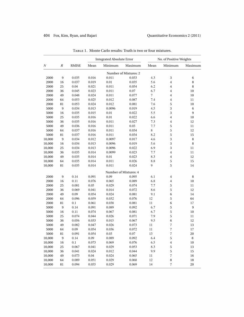
We summarize our results in Table 1, where the true distribution has two or fourcomponents, and in Table 2, where the true distribution has six components. The firsttwo columns report the sample size N and the number R of basis points used in theestimation. The next column reports the RMISE of the estimated distribution functions.The following three columns reports the mean, minimum, and maximum of the IAE.The final three columns report the mean, minimum, and maximum of the number ofbasis functions that have positive weight.
404 Fox, Kim, Ryan, and Bajari Quantitative Economics 2 (2011)
Table 1. Monte Carlo results: Truth is two or four mixtures.
Integrated Absolute Error No. of Positive Weights
N R RMISE Mean Minimum Maximum Mean Minimum Maximum
Number of Mixtures: 22000 9 0�035 0�016 0�011 0�033 4�3 3 62000 16 0�037 0�019 0�01 0�035 5�6 4 82000 25 0�04 0�021 0�011 0�054 6�2 4 82000 36 0�045 0�023 0�011 0�07 6�7 4 102000 49 0�048 0�024 0�011 0�077 7 4 102000 64 0�053 0�025 0�012 0�087 7�4 4 112000 81 0�053 0�024 0�012 0�081 7�6 5 105000 9 0�034 0�013 0�0096 0�019 4�5 3 65000 16 0�035 0�015 0�01 0�022 5�5 3 95000 25 0�035 0�016 0�01 0�022 6�6 4 105000 36 0�035 0�016 0�011 0�027 7�3 4 125000 49 0�036 0�016 0�011 0�03 7�7 5 115000 64 0�037 0�016 0�011 0�034 8 5 125000 81 0�037 0�016 0�011 0�034 8�2 5 15
10,000 9 0�034 0�012 0�0097 0�017 4�6 3 810,000 16 0�034 0�013 0�0096 0�019 5�6 3 810,000 25 0�034 0�013 0�0096 0�022 6�9 3 1110,000 36 0�035 0�014 0�0099 0�023 7�7 4 1110,000 49 0�035 0�014 0�01 0�023 8�3 4 1210,000 64 0�035 0�014 0�011 0�026 8�8 5 1510,000 81 0�035 0�014 0�011 0�024 9 5 14
Number of Mixtures: 42000 9 0�14 0�091 0�09 0�095 6�1 4 82000 16 0�11 0�076 0�065 0�089 6�8 4 102000 25 0�081 0�05 0�029 0�074 7�7 5 112000 36 0�069 0�041 0�014 0�072 8�6 5 122000 49 0�09 0�054 0�024 0�081 9�1 6 142000 64 0�096 0�059 0�032 0�076 12 5 642000 81 0�1 0�061 0�038 0�081 11 6 175000 9 0�14 0�091 0�089 0�092 6�7 5 95000 16 0�11 0�074 0�067 0�081 6�7 5 105000 25 0�074 0�044 0�026 0�071 7�9 5 115000 36 0�056 0�033 0�015 0�067 9�5 6 125000 49 0�082 0�047 0�026 0�073 11 7 135000 64 0�09 0�054 0�036 0�072 11 7 175000 81 0�091 0�054 0�03 0�07 13 7 20
10,000 9 0�14 0�09 0�089 0�092 6�4 5 810,000 16 0�1 0�073 0�069 0�076 6�5 4 1010,000 25 0�067 0�041 0�029 0�053 8�3 5 1310,000 36 0�041 0�024 0�012 0�044 9�9 5 1510,000 49 0�073 0�04 0�024 0�065 11 7 1610,000 64 0�089 0�051 0�029 0�068 12 8 1810,000 81 0�094 0�055 0�029 0�069 14 7 20

Quantitative Economics 2 (2011) Distribution of random coefficients 405
Table 2. Monte Carlo results: Truth is six mixtures.
Integrated Absolute Error No. of Positive Weights
N R RMISE Mean Minimum Maximum Mean Minimum Maximum
Number of Mixtures: 62000 9 0�2 0�15 0�14 0�16 6�1 5 72000 16 0�11 0�07 0�064 0�093 9�7 7 122000 25 0�12 0�087 0�064 0�099 10 7 232000 36 0�057 0�04 0�016 0�063 12 8 152000 49 0�092 0�065 0�054 0�079 13 9 172000 64 0�082 0�059 0�043 0�085 14 10 192000 81 0�072 0�052 0�029 0�083 15 11 235000 9 0�19 0�15 0�14 0�15 6�2 5 75000 16 0�11 0�069 0�065 0�088 10 7 125000 25 0�12 0�09 0�082 0�096 9�7 7 115000 36 0�045 0�03 0�018 0�053 13 8 165000 49 0�091 0�063 0�052 0�075 13 9 165000 64 0�075 0�053 0�04 0�074 15 11 195000 81 0�068 0�05 0�037 0�068 17 9 23
10,000 9 0�19 0�15 0�15 0�15 6�2 5 710,000 16 0�11 0�069 0�064 0�075 10 7 1310,000 25 0�12 0�09 0�079 0�098 10 8 1410,000 36 0�043 0�028 0�014 0�057 13 8 1810,000 49 0�091 0�062 0�055 0�07 14 9 1810,000 64 0�073 0�051 0�044 0�066 15 11 2310,000 81 0�067 0�05 0�039 0�067 17 11 24
The results in Tables 1 and 2 suggest that our estimator of F(β) exhibits excellentperformance, even in relatively small samples. By and large, RMISE and IAE are rela-tively low and decrease with N and R. Note that we are able to fit the underlying distri-bution functions well with a fairly small number of basis functions. While performancegenerally increases with the number of basis functions, it is worth noting that the fit candecrease with increases in R, as the grids do not nest each other for marginal increasesinR. This is apparent in this sample forN = 2000, where smallerR’s have lower RMISE’s.The mean number of nonzero basis functions ranges from 4 to 17, with more complextrue distributions requiring more nonzero basis points for approximation. This result isconsistent with the literature on mixtures, which demonstrates that complicated distri-butions can be approximated with a surprisingly small number of mixture components.
We plot the estimated marginal distributions of both β1 and β2. Figure 1 includesone plot for each of the three designs and each of the two random coefficients. For com-parison, we also include a plot of a bivariate normal fitted to the same data sets usingmaximum likelihood, along with the 5th and 95th quantiles of the estimated distribu-tions at each point of evaluation. The general fits of our current estimator are excel-lent; the discrete distribution tracks the CDF of the underlying model uniformly well.The variability across replications is quite low at this sample size, and the true CDF lieswithin the 90 percent confidence bands with the small exception of boundary values

406 Fox, Kim, Ryan, and Bajari Quantitative Economics 2 (2011)
Figure 1. Marginal distribution of β1 and β2 withN = 10�000 and R= 81.
where the discrete CDF jumps. On balance, our estimator consistently recovers the truemarginal distributions of the two coefficients.
Figures 2 and 3 plot the true versus the estimated joint distribution (using one ofour replications) of the model with six mixtures. Here R = 81 and N = 10�000. A visualinspection of the distributions shows that we are able to generate excellent fits to thetrue distribution functions of preferences using our estimator. For comparison, Figure 4is a plot of the estimation error. The sawtooth nature of the error plot is driven by the factthat the discrete approximation to the CDF results in step functions, which then implythat the errors have discontinuities at the basis points. Our estimator produces a goodapproximation to the underlying distribution function even with limited data and whenthe number of basis points is small.
In Table 3, we report the results for a bivariate normal distribution with a nonzerocorrelation parameter run on the same data sets. The bivariate normal has a RMISE andan IAE noticeably larger than our values. The fit does not improve with an increase in

Quantitative Economics 2 (2011) Distribution of random coefficients 407
Figure 2. True distributions for six mixtures.
the number of observations. As can be seen in the graphs of the marginal densities inFigure 1, the bivariate normal distribution simply cannot match the shape of the un-derlying true CDF. Interestingly, it has a better fit on the true models with more mixture
Figure 3. Fitted distributions for six mixtures withN = 10�000 and R= 81.

408 Fox, Kim, Ryan, and Bajari Quantitative Economics 2 (2011)
Figure 4. Error in fitted distribution for six mixtures withN = 10�000 and R= 81.
components, as the underlying CDF has more features and on average is closer in shapeto the bivariate normal. In all cases, however, our estimator dominates the performanceof the bivariate normal.
We also experimented with using a random grid to populate the basis points.10 Therandom grid exhibited much poorer convergence properties than the uniform grid, pri-
Table 3. Monte Carlo results: Bivariate normal maximum likelihood.
Integrated Absolute Error
N RMISE Mean Minimum Maximum
Number of Mixtures: 2
2000 0.29 0�24 0�19 0.315000 0.3 0�25 0�2 0.31
10,000 0.3 0�25 0�2 0.3
Number of Mixtures: 42000 0.15 0�082 0�066 0.125000 0.15 0�078 0�07 0.088
10,000 0.16 0�074 0�07 0.086
Number of Mixtures: 62000 0.18 0�094 0�09 0.15000 0.18 0�094 0�088 0.1
10,000 0.19 0�095 0�089 0.11
10Results available from authors on request.

Quantitative Economics 2 (2011) Distribution of random coefficients 409
marily due to the fact that there are no guarantees in small samples (with correspond-ingly small numbers of basis points) that the grid will have good coverage over the rele-vant areas of the parameter space. For this reason, we suggest the use of a uniform gridwhen data and computational limits allow it.
8. Empirical application to dynamic programming
As an illustration of our estimator, we apply it to the dynamic labor supply setting fromDuflo, Hanna, and Ryan (forthcoming), hereafter referred to as DHR. They consideredthe problem of incentivizing teachers to go to work and estimated a dynamic laborsupply model using the method of simulated moments. The model is a single agent,dynamic programming problem with a serially correlated, unobserved state variable.To accommodate unobserved heterogeneity across teachers, they estimated a two-typemixture model. We apply the present estimator to this setting and show that our ap-proach allows for a more flexible approximation of the underlying heterogeneity. Fur-ther, our new estimator is quicker to run and easier to implement.
Teacher absenteeism is a major problem in India, as nearly a quarter of all teach-ers are absent nationwide on any given day. The absenteeism rate is nearly 50 percentamong nonformal education centers, nongovernment-run schools designed to provideeducation services to rural and poor communities. To address absenteeism, DHR rana randomized field experiment where teachers were given a combination of monitor-ing and financial incentives to attend school. In a sample of 113 rural, single-teacherschools, 57 randomly selected teachers were given a camera and told to take two picturesof themselves with their students on days they attend work. On top of this monitoringincentive, teachers in the treatment group also received a strong financial incentive: forevery day beyond 10 they worked in a month, they received a 50 rupee bonus on topof their baseline salary of 500 rupees a month. The typical work month in the samplewas about 26 days, so teachers who went to school at every opportunity received greaterwages than the control group, who were paid a flat amount of 1000 rupees per month.The program ran for 21 months and complete work histories were collected for all teach-ers over this period.
DHR evaluated this program and found the combination of incentives was success-ful in reducing absenteeism from 42 percent to 21 percent. To disentangle the confound-ing effects of the monitoring and financial incentives, they exploited nonlinearities inthe financial incentive to estimate the labor supply function of the teachers.
A convenient aspect of the intervention is that the financial incentives reset eachmonth. Therefore, the model focused on the daily work decisions of teachers within amonth. Denote the number of days it is possible to work in each month asC. Let t denotethe current day and let the observed state variable d denote the number of days alreadyworked in the month. Each day a teacher faces a choice of going to school or stayinghome. The payoff to going to school is zero. The payoff to staying home is equal to μi +εi�t , where μi is specific to teacher i and εi�t is a shock to payoffs. The shock εi�t is seriallycorrelated.

410 Fox, Kim, Ryan, and Bajari Quantitative Economics 2 (2011)
After the end of the month (C), the teachers receive the following payoffs, denom-inated in rupees, which are a function of how many days d that teacher worked in themonth:
π(d)={
500 + (10 − d) · 50� if d ≥ 10,500� otherwise.
Let r be the type of the teacher in our approximation. The choice decision facing eachteacher in the form of a value function for periods t < C is
V r(t� di� εi�t) = max{E
[V r(t + 1� di + 1� εi�t+1) | εi�t
]�
μr + εi�t +E[V r(t + 1� di� εi�t+1) | εi�t
]}�
At time C, the value function simplifies to
V r(C�di� εi�C)= max{βπ(di + 1)�μr + εi�C +βπ(di)
}� (16)
where β is the marginal utility of an additional rupee. There is no continuation value inthe right side of (16) as the stock of days worked resets to zero at the end of the month.These value functions illustrate the trade-off teachers face early in each month betweenaccruing days worked, in the hope of receiving an extra payoff at the end of the month,and obtaining instant gratification by skipping work.11
DHR proposed a simulated method of moments estimator that matches sequencesof days worked at the beginning of each month. They found parameters that generatepredicted probabilities for all the possible sequences of work histories in the first fivedays of each month as close as possible to their empirical counterparts.12 This pro-cedure resulted in 25 − 1 = 31 linearly independent moments to be matched in eachmonth. They estimated several specifications of the above model using this approach;we focus on their preferred model, in which the shock to the outside option follows anAR(1) process with correlation parameter ρ and the teacher-specific deterministic com-ponent of the outside option μi is drawn from a bimodal normal distribution. Note thatthis is a very computationally intensive problem, as the researcher must integrate outover both the distribution of outside options μi and the serially correlated unobservableεi�t to produce the probabilities of sequences of days worked. The model requires sev-eral hundred thousand simulations to produce estimates of the probabilities of workingsequences with low variance for each type. Using a two-type mixture estimated using
11The day of the month t and stock of worked days d are naturally discrete state variables. For eachcombination of t and d, the continuous state ε is discretized into 200 bins. For each simulated value of ε, theclosest bin value is taken to be the actual state for the purposes of dynamic programming. For numericalintegration in the calculation of expectations such as E[V r(t + 1� di + 1� εi�t+1) | εi�t ], the distribution ofεi�t+1 is used to calculate the probability εi�t+1 lies in each of the 200 bins, and those probabilities weightV r(t + 1� di + 1� εi�t+1) in the approximation to the expectation.
12Considering data on only the first five days in each month both simplifies the computational burdenand breaks much of the statistical dependence across the beginning of months (as the correlation of εi�tacross months is low). We treat data from different months as statistically distinct from the viewpoint of thecorrelation in εi�t .

Quantitative Economics 2 (2011) Distribution of random coefficients 411
the method of simulated moments, DHR estimated that in a given month 97.6 percentof the teachers have outside options drawn from a normal distribution with a mean of−0.428 and a variance of 0.007, and the remaining 2.4 percent of teachers have outsideoptions drawn from a normal distribution with mean 1.781 and variance 0.050. At theestimated parameters of this model, workers who draw the first distribution generallygo to school every day, while workers who draw from second distribution are likely tonever attend school during a given month.
There are natural bounds on the level of the outside option, as low values of μi leadto teachers always working and high values lead to teachers never working. The auto-correlation parameter is bounded between −1 and +1. The β parameter is also sharplybounded, as its effects on work behavior are similar to the outside option, outside a nar-row range.
We apply the present paper’s estimator to this setting, allowing for a more flexibledistribution of heterogeneity in the outside option. We hold the marginal utility of in-come and the autocorrelation parameter at their values estimated under the two-typemodel in DHR: β= 0�013 and ρ= 0�449.13
We estimate the model with a discrete approximation to the distribution of hetero-geneity in the outside option. We let the number of basis functions range betweenR= 5and R = 40, with the types uniformly distributed across the economic bounds on theoutside option. At the lower extreme, μi = −2�5, the teachers almost always go to work,and at the upper extreme,μi = 4�0, teachers almost never go to work. We solve the modelunder each of those R draws for every month in the data set. In addition to the intra-month time series variation in the moments, our model is identified from variation inthe number of days, the distribution of workdays (teachers receive one day off on theweekends), and the number of holidays, which count as a day worked in the teacher’spayoff function, across months. These exogenous sources of variation produce differentprobabilities of working even under the same set of model primitives.
For each month in the data, we solve the dynamic program for all R types andthen compute the probabilities of all possible sequences of days worked in the first fivedays of the month. We collate these probabilities together to produce a matrix with Rcolumns and 31 = 25 − 1 rows, where each row corresponds to the probability of observ-ing a specific work history for that month. We then stack these matrices across months toobtain a large matrix withR columns and 31∗21 = 651 rows corresponding to the 31 pos-sible work histories and the 21 different months. We formed the corresponding vector ofempirical probabilities as the vector of dependent variables. We then estimated weightsfor each of the R types using the inequality constrained least-squares estimator.14 Thisestimator is similar to the specification in equation (12), except that we do not use panel
13In a previous draft of the paper, we also experimented with allowing for unobserved heterogeneity inthe other two parameters—the marginal utility of income (β) and the degree of persistence in the AR(1)process (ρ), with unrestricted covariance across the parameters. We found that the β and ρ parameterswere always estimated tightly around their point estimates and, therefore, we focus on the distribution ofμi in what follows.
14We use a penalized (for the constraints) Newton method to minimize the least-squares objective func-tion. We use the assumption that the true types are the types included to construct confidence intervals,as in Section 6. Confidence intervals are constructed using the standard OLS formulas. An observation is

412 Fox, Kim, Ryan, and Bajari Quantitative Economics 2 (2011)
Figure 5. Estimated distributions of heterogeneity for the benefits of staying home.
data to construct sequences of choices for the same teacher across months, only withinmonths.
The estimated distributions of types are shown in Figure 5. The vertical axis is theweight of that type in the probability mass function that is an approximation to thetrue distribution of types. The squares represent the point estimates; the sum of theseweights is always 1. The figures also show the 90% confidence intervals for the weight oneach type. The confidence intervals are smaller in the center of the distribution. Keepin mind that these are univariate confidence regions for individual weights; the confi-dence regions for functions of all of the weights, such as F(β) at a particular β, may berelatively narrower. In these and subsequent figures, we present four approximations:R = 5, 10, 20, and 40. The R = 40 estimates suggest a double-peaked distribution of autility of staying home in the range from −0.5 to 0.0. Three basis points in the range−0.5–0.0 are given substantial weight. The right tail is thin: most weights are 0, but the
a teacher/month. Five days are used for each teacher/month observation. The number of observations is1123 teacher/months. The correlation in εi�t across the first five days should be low, so we do not accountfor autocorrelation across teacher/months for the same teacher.
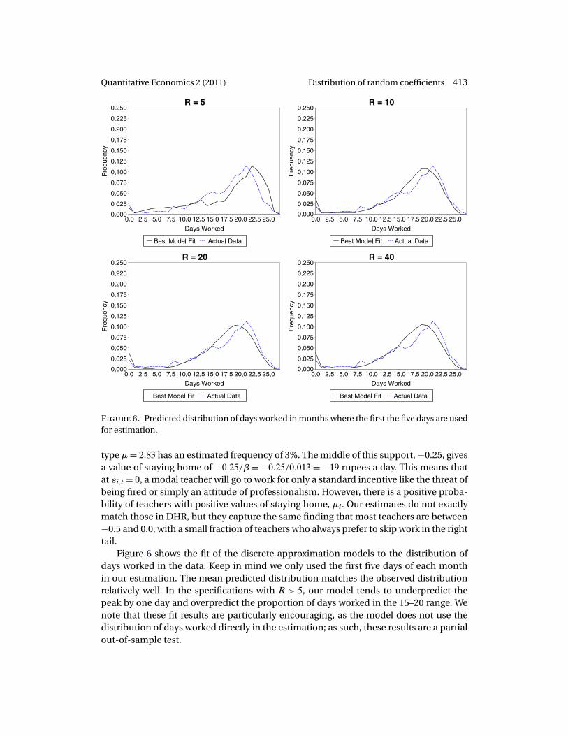
Quantitative Economics 2 (2011) Distribution of random coefficients 413
Figure 6. Predicted distribution of days worked in months where the first the five days are usedfor estimation.
type μ= 2�83 has an estimated frequency of 3%. The middle of this support, −0.25, givesa value of staying home of −0�25/β = −0�25/0�013 = −19 rupees a day. This means thatat εi�t = 0, a modal teacher will go to work for only a standard incentive like the threat ofbeing fired or simply an attitude of professionalism. However, there is a positive proba-bility of teachers with positive values of staying home, μi. Our estimates do not exactlymatch those in DHR, but they capture the same finding that most teachers are between−0.5 and 0.0, with a small fraction of teachers who always prefer to skip work in the righttail.
Figure 6 shows the fit of the discrete approximation models to the distribution ofdays worked in the data. Keep in mind we only used the first five days of each monthin our estimation. The mean predicted distribution matches the observed distributionrelatively well. In the specifications with R > 5, our model tends to underpredict thepeak by one day and overpredict the proportion of days worked in the 15–20 range. Wenote that these fit results are particularly encouraging, as the model does not use thedistribution of days worked directly in the estimation; as such, these results are a partialout-of-sample test.

414 Fox, Kim, Ryan, and Bajari Quantitative Economics 2 (2011)
Figure 7. Predicted distribution of days worked under the out-of-sample compensationscheme.
A feature of the teacher data is that there is a completely independent second exper-iment, which was conducted after the first intervention, in which the incentives facingteachers were changed. Instead of working 10 days to get a marginal per-day bonus of50 rupees, teachers in the second experiment had to work 12 days to get a marginal per-day bonus of 70 rupees. Figure 7 shows the fits of the discrete approximation models inthe out-of-sample test. These data are a bit noisier than the original data set, due to asmaller sample size, but the model also does a fairly good job of matching the distribu-tion of days worked. Our approach tends to underpredict the proportion of zero daysworked and overpredict the number of days worked above 18.
It is worth emphasizing that the computational burden of the present estimator ismuch lower than the alternative used in DHR. We ran several timing tests to evalu-ate the performance of our estimator against alternatives used in DHR. We tabulatedthe time it took our estimator to run from start to finish while varying the number ofpoints in the discrete support, R ∈ {5�10�20�40}, and the number of simulations used tosimulate the conditional moments (here probabilities of labor supply histories) in bothour estimator and the generalized method of moments (GMM) estimator used in DHR,

Quantitative Economics 2 (2011) Distribution of random coefficients 415
Table 4. Run times in seconds of our estimator and the two-type GMM estimator used in DHR.a
Number of Simulationsin ConditionalLabor Supply HistoryProbabilities
Two-Type GMM Our EstimatorStarting Values Number of Basis Points R
DHR Optimum No Heterogeneity 5 10 20 40
S = 2000 282 640 11.5 35.4 44.1 64.8S = 20�000 1010 2360 33 67 120 242S = 200�000 87,800 110,000 280 555 978 1960
aThe objective functions for both estimators were minimized using the nonlinear solver KNITRO.
S ∈ {2000�20�000�200�000}. In the GMM estimator, we let the distribution of marginalutility be drawn from a single normal distribution. We set the number of draws from thatdistribution to be equal to 128 when computing the conditional moments. We startedthe GMM alternative with two sets of starting values. The first starting value was set atthe parameter values from a model without heterogeneity on the coefficient of stayinghome, where we set the variance of the distribution on the value of staying home to beequal to 1. In the second experiment, we set the starting value to be the optimized valuein DHR. In the second case, the optimizer simply has to verify that the starting value is alocally optimal solution and should reflect the lowest possible burden in computing thesolution to the model.
Table 4 reports the run times for the two-type GMM and our estimators. For S = 2000and S = 20�000, our estimator with R= 40 is around four times faster than the GMM es-timator started at the converged parameter vector from DHR. It is over 40 times fasterwhen S = 200�000. When the GMM estimator used in DHR is not started at the final vec-tor, the R= 40 speed advantage of our estimator is between 10 and 55 times faster thanthe alternative. An interesting feature to highlight is that adding complexity to our modelis essentially a linear operation; doubling the number of basis points roughly doublesthe execution time. Also, as all of our run time is spent evaluating probabilities for dif-ferent consumer types β, our approach is easy to parallelize across multiple processors.
9. Conclusion
In this paper, we have proposed a new method for estimating general mixtures models.In terms of computer programming and execution time, our linear regression estimatoris easier to work with than simulated likelihood or method of moments estimators. Con-vergence of an optimization routine to the global optimum is guaranteed under linearregression with linear inequality constraints, something that cannot be said for otherstatistical objective functions. Also, our estimator is easier to program and to use thanalternatives such as the EM algorithm.
Our estimator is useful for estimating a wide variety of models. In a dynamic pro-gramming setting, the estimator allows for a distribution of random coefficients whilesimultaneously cutting the computational time even compared to the model withoutrandom coefficients. Our approach has dramatic computational savings compared to

416 Fox, Kim, Ryan, and Bajari Quantitative Economics 2 (2011)
other estimators for a dynamic programming model with random coefficients. The com-putational savings arise because we must solve the dynamic program only once for eachbasis vector.
We apply our estimator in an empirical example of estimating the distribution ofagent preferences in a dynamic programming model with an unobserved, serially cor-related state variable. Our estimator uses less programming and execution time than analternative simulation estimator.
References
Ackerberg, D. A. (2009), “A new use of importance sampling to reduce computa-tional burden in simulation estimation.” Quantitative Marketing and Economics, 7 (4),343–376. [396]
Andrews, D. K. W. (1999), “Estimation when a parameter is on a boundary.” Economet-rica, 67, 1341–1383. [402]
Andrews, D. K. W. (2000), “Inconsistency of the bootstrap when a parameter is on theboundary of the parameter space.” Econometrica, 68, 399–405. [402]
Andrews, D. K. W. (2002), “Generalized method of moments estimation when a parame-ter is on a boundary.” Journal of Business & Economic Statistics, 20 (4), 530–544. [387, 402]
Andrews, D. K. W. and P. Guggenberger (2009), “Hybrid and size-corrected subsamplemethods.” Econometrica, 77 (3), 721–762. [402]
Andrews, D. K. W. and P. Guggenberger (2010a), “Applications of subsampling, hybrid,and size-correction methods.” Journal of Econometrics, 158, 285–305. [401, 402]
Andrews, D. K. W. and P. Guggenberger (2010b), “Asymptotic size and a problem withsubsampling and them out of n bootstrap.” Econometric Theory, 26, 426–468. [402]
Beran, R. and P. W. Millar (1994), “Minimum distance estimation in random coefficientregression models.” The Annals of Statistics, 22 (4), 1976–1992. [384]
Berry, S. and P. Haile (2010a), “Identification in differentiated products markets usingmarket level data.” Working paper, NBER. [398]
Berry, S. and P. Haile (2010b), “Nonparametric identification of multinomial choice de-mand models with heterogeneous consumers.” Working paper, NBER. [383, 398]
Berry, S., J. Levinsohn, and A. Pakes (1995), “Automobile price in market equilibrium.”Econometrica, 63 (4), 841–890. [383, 398, 400]
Berry, S., O. Linton, and A. Pakes (2004), “Limit theorems for estimating the parametersof differentiated product demand systems.” Review of Economic Studies, 71 (3), 613–654.[400]
Biernacki, C., G. Celeux, and G. Govaert (2003), “Choosing starting values for the EMalgorithm for getting the highest likelihood in multivariate Gaussian mixture models.”Computational Statistics & Data Analysis, 41, 561–575. [384]

Quantitative Economics 2 (2011) Distribution of random coefficients 417
Böhning, D. (1982), “Convergence of Simar’s algorithm for finding the maximum like-lihood estimate of a compound Poisson process.” The Annals of Statistics, 10 (3),1006–1008. [383]
Burda, M., M. Harding, and J. Hausman (2008), “A Bayesian mixed logit–probit for multi-nomial choice demand models.” Journal of Econometrics, 147 (2), 232–246. [383]
Dempster, A. P., N. M. Laird, and D. B. Rubin (1977), “Maximum likelihood from incom-plete data via the EM algorithm.” Journal of the Royal Statistical Society, 39 (1), 1–38.[383]
Dubin, J. A. and D. L. McFadden (1984), “An econometric analysis of residential electricappliance holdings and consumption.” Econometrica, 52 (2), 345–362. [396]
Duflo, E., R. Hanna, and S. P. Ryan (forthcoming), “Monitoring works: Getting teachersto come to school.” American Economic Review. [384, 409]
Fox, J. T. and A. Gandhi (2010), “Nonparametric identification and estimation of ran-dom coefficients in nonlinear economic models.” Working paper, University of Michi-gan. [383, 385, 398]
Fox, J. T. and A. Gandhi (2011a), “Using selection decisions to identify the joint distribu-tion of outcomes.” Working paper, University of Michigan. [396]
Fox, J. T. and A. Gandhi (2011b), “Identifying Demand With Multidimensional Unob-servables: A Random Functions Approach.” Working paper, University of Michigan.[383, 398]
Geweke, J. (1986), “Exact inference in the inequality constrained normal linear regres-sion model.” Journal of Applied Econometrics, 1 (2), 127–141. [401]
Golub, G. H., M. Heath, and G. Wahba (1979), “Generalized cross-validation as a methodfor choosing a good ridge parameter.” Technometrics, 21 (2), 215–223. [401]
Hansen, B. (2004), “Bandwidth selection for nonparametric distribution estimation.”Working paper, University of Wisconsin. [389]
Heckman, J. J. (1981), “The incidental parameters problem and the problem of initialconditions in estimating a discrete time-discrete data stochastic process.” In StructuralAnalysis of Discrete Data With Econometric Applications (C. Manski and D. McFadden,eds.), Ch. 4, 179–195, MIT Press, Cambridge. [395]
Heckman, J. and B. Singer (1984), “A method for minimizing the impact of distributionalassumptions in econometric models for duration data.” Econometrica, 52 (2), 271–320.[383]
Judge, G. G. and T. Takayama (1966), “Inequality restrictions in regression analysis.” Jour-nal of the American Statistical Association, 61 (313), 166–181. [401]
Kamakura, W. A. (1991), “Estimating flexible distributions of ideal-points with externalanalysis of preferences.” Psychometrika, 56 (3), 419–431. [384]

418 Fox, Kim, Ryan, and Bajari Quantitative Economics 2 (2011)
Karlis, D. and E. Xekalaki (2003), “Choosing initial values for the EM algorithm for finitemixtures.” Computational Statistics & Data Analysis, 41, 577–590. [384]
Kim, K. and A. Petrin (2010), “Control function corrections for unobserved factors indifferentiated product models.” Working paper, University of Minnesota. [383, 398]
Laird, N. (1978), “Nonparametric maximum likelihood estimation of a mixing distribu-tion.” Journal of the American Statistical Association, 73 (364), 805–811. [383]
Li, J. Q. and A. R. Barron (2000), “Mixture density estimation.” Advances in Neural Infor-mation Processing Systems, 12, 279–285. [384]
Liew, C. K. (1976), “Inequality constrained least-squares estimation.” Journal of theAmerican Statistical Association, 71 (355), 746–751. [401]
Lindsay, B. G. (1983), “The geometry of mixture likelihoods: A general theory.” The An-nals of Statistics, 11 (1), 86–94. [383]
McLachlan, G. J. and D. Peel (2000), Finite Mixture Models. Wiley, New York. [384]
Newey, W. K. and D. McFadden (1994), “Large sample estimation and hypothesis test-ing.” In Handbook of Econometrics, Volume 4, 2111–2245, Elsevier, Amsterdam. [387]
Pilla, R. S. and B. G. Lindsay (2001), “Alternative EM methods for nonparametric finitemixture models.” Biometrika, 88 (2), 535–550. [384]
Politis, D. N., J. P. Romano, and M. Wolf (1999), Subsampling. Springer, New York. [402]
Quandt, R. E. and J. B. Ramsey (1978), “Estimating mixtures of normal distributions andswitching regressions.” Journal of the American Statistical Association, 73 (364), 730–738.[384]
Rossi, P. E., G. M. Allenby, and R. McCulloch (2005), Bayesian Statistics and Marketing.John Wiley & Sons, West Sussex. [383]
Rust, J. (1987), “Optimal replacement of GMC bus engines: An empirical model of HaroldZurcher.” Econometrica, 55 (5), 999–1033. [383, 394]
Rust, J. (1994), “Structural estimation of Markov decision processes.” In Handbook ofEconometrics, Volume 4 (R. F. Engle and D. L. McFadden, eds.), North-Holland, Amster-dam. [394]
Seidel, W., K. Mosler, and M. Alker (2000), “A cautionary note on likelihood ratio tests inmixture models.” Annals of the Institute of Statistical Mathematics, 52 (3), 418–487. [384]
Verbeek, J. J., N. Vlassis, and B. Kröse (2003), “Efficient greedy learning of Gaussian mix-ture models.” Neural Computation, 15, 469–485. [384]
Wolak, F. (1989), “Testing inequality constraints in linear econometric models.” Journalof Econometrics, 41 (2), 205–235. [401]
Submitted January, 2010. Final version accepted June, 2011.