A simple model of eating decisions and weight with

rational and forward-looking agents

Sebastien Buttet∗ and Veronika Dolar†

January 18, 2010

Abstract

Several empirical papers in the economics of obesity literature find that changes

in aggregate food prices over time have little effect on the population body-mass

index or obesity prevalence, while changes in the price of selected food items dras-

tically affects what people eat. We propose a simple dynamic model with rational

agents to further examine the impact of changes in food prices and household real

income on eating decisions and weight of men and women between 1971 and 2006.

We also introduce a new measure for food prices which considers the price per calo-

rie consumed rather than prices of specific food items. After careful calibration

of the model using evidence from medical research on obesity, we find that prices

determine the allocation of calories across food types, while income determine the

total number of calories consumed and thus individuals’ weight. Based on our re-

sults, we share the view that taxes on food will impact what people eat but will have

limited effect on reducing the population body-mass index or the obesity prevalence.

JEL Classification: I10, D91

Keywords: Obesity, body weight, food prices.

∗Cleveland State University. Email: s.buttet@csuohio.edu.†University of Minnesota. Email: dola0068@umn.edu. All errors are ours.

1

1 Introduction

Two decades of intense research in the field of economics of obesity have improved our

understanding of the impact of food prices on weight and food choices and two critical

results have gained wide acceptance. First, several empirical studies show that changes

in aggregate food prices over time have little effect on the population body-mass index or

obesity prevalence (e.g., Chou et al., 2004, Gelbach et al., 2007). Second, experimental

studies show that changes in the price of selected food items drastically affects what people

eat. For example, French, Jeffery, Story, Breitlow, Baxter, Hannan, and Snyder (2001)

find that a fifty percent price reduction on low-fat snacks in vending machines at schools

and work places increase the percentage of low-fat snack sales by ninety three percent.

These two results about the (lack of) effect of food prices on weight and food choices are

important because of their influence on the public health debate about the effectiveness

of fiscal policies for winning the fight against the obesity epidemic. A common view held

by policymakers is that taxes applied selectively to different food items work effectively

to reduce consumption of a particular type of food or ingredient (e.g., ban of trans-fats

in New-York City) but are unlikely to produce significant changes in body-mass index or

obesity prevalence (Powell and Chaloupka, 2009 and Chouinard et al., 2007).

In this paper, we further examine the impact of changes over time in food prices and

household real income on individuals’ food choices and weight using a calibrated dynamic

model. Our first objective is to contribute to the debate about the impact of food prices

and household real income on weight and food choices using a different modeling strategy.

Using our calibrated model, we ask how much of the increase in calories consumed away

from home as well as changes in weight for men and women in different age groups between

1971 and 2006 can be accounted for by changes in food prices and household real income.

A second and perhaps even more critical objective is to use economic theory and available

evidence from medical research on obesity to look inside the black box of how people

make eating decisions, in particular improve our understanding of what determines the

(low) food price elasticity of weight.

Our environment for studying eating decisions and weight accumulation rests upon

the following assumptions. First, we use economic theory to model agents’ food choices,

2

including the total number of calories consumed every day as well as the fraction of calories

consumed at home versus away from home. We posit that agents are fully rational and

forward-looking. Given household real disposable income and the relative price of a calorie

(at home versus away from home), agents decide how much to eat at each location as well

as how much of the non-food good to consume to maximize a well-defined objective

function. Second, we use medical research on nutrition to link daily calorie intake to

weight gain. We assume that weight is a stock variable and calorie intake a flow variable.

A weight law of motion relates weight in future periods to weight and food decisions in the

current period. Agents gain (lose) weight when total calorie consumption in the current

period is greater (less) than the number of calories required to maintain current weight

that depends on the agent’s age and is greater for men compared to women. Finally, we

use medical research on obesity-related diseases to link agent’s weight to her longevity.

We assume that a positive probability exists in each period that agents die and that

this probability depends on the agent’s body-mass index. We consider the case where

the survival probability is an inverted U-shape function of body-mass index, implying

that agents who are either over- or underweight have a greater chance to die. As a result,

agents arbitrate the following simple trade-off to smooth utility over time. Increasing food

consumption in the current period yields instantaneous utility but also leads to higher

weight and increased mortality risks in the future.

We concentrate our analysis on the following facts about weight and calories consumed

away from home to evaluate the impact of food prices and income within our model. First,

the average weight of adult men and women increased by twenty-two and twenty-three

pounds, respectively between 1971 and 2006. Second, the fraction of total daily calories

consumed away from home increased from thirty to forty percent for adult men and from

eighteen to thirty-five percent for adult women over the same period of time. Finally, we

document changes in average weight and calories away from home for men and women

in different age groups between 1971 and 2006. Note that gender and age play two key

roles in our analysis of weight and food choices reflecting economic and physiological

differences between men and women and over the life-cycle. One the physiological side,

men can afford to eat more calories every day compared to women without gaining weight.

3

The relationship between calorie intake and weight also differs along the life-cycle. As

individuals age, the number of calories needed to maintain a constant weight declines

(see a technical report (2002) published by the Food and Nutrition Board of the Institute

of Medicine of the National Academies). On the economic side, household real income

fluctuates over the life-cycle influencing food choices and thus weight.

We introduce a new measure for food prices which considers the price per calorie

consumed rather than prices of specific food items. Using data on food expenditures as

well as calories consumed from the US Department of Agriculture between 1971 and 2006,

we calculate price per calorie for food consumed away from home and food consumed at

home as the dollar amount spent by households on each food category divided by the

number of calories consumed at each location. We find that the relative price per calorie

(away from home versus at home) declined by seventeen percent, while household real

income increased by twenty-four percent over the same period of time. We use our newly

constructed time series for price per calorie as an input into our dynamic model.

Results for the impact of food prices and household income on individuals’ food choices

and weight are only interesting and credible if we can justify the choice of the model pa-

rameters unequivocally. We use available evidence from medical research on nutrition to

calibrate the weight law of motion and medical research on obesity-related diseases to

fix the survival probability function. We choose the remaining preferences parameters to

match the mean weight and fraction of calories away from home observed in NHANES

1971-75, allowing some preference heterogeneity between men and women. Using our cal-

ibrated model, we find that changes in food prices and real income affect eating decisions

and weight differently. In a nutshell, prices determine the allocation of calories across food

types, while income determine the total number of calories consumed. Taken altogether,

however, changes in per calorie food prices and real income account for a large share of

the increase in weight and the fraction of calories consumed away from home for men and

women in different age groups between 1971 and 2006.

Our results corroborate the existing scientific knowledge about food choices and obe-

sity. Using a fully specified calibrated dynamic model (as opposed to econometrics or field

experiments) and time series (as opposed to cross-section) data, we show that changes

4

in food prices over time account for almost none of the weight gain by Americans men

and women in the last thirty years and for more than fifty percent of the increase in

calories consumed away from home by men and women. As such, we support the view

that taxes on food will impact what people eat but will have limited effect on reducing

the population body-mass index or the obesity prevalence.1

The remainder of the paper is organized as follows. In Section 2, we describe data

about weight, calories consumed away from home, per calorie food prices and household

real income between 1971 and 2006. In Section 3 and Section 4, we develop and cali-

brate our dynamic model and we conduct our simulations in Section 5. Finally, we offer

concluding remarks in Section 6.

2 Nutritional and Economic Data

In this section, we use two distinct sample data from the National Health and Nutritional

Examination Survey (NHANES) to document changes over time in body-mass index,

weight, and the fraction of calories consumed away from home for men and women for

the period between 1971 and 2006 (see Table 1).2 Data about weight comes from the

examination component of NHANES and is measured by trained medical personnel. The

fraction of calories consumed away from home, on the other hand, is self-reported by

individuals.3

1Note that distortionary taxes on food will result in sub-optimal allocations when agents are fully ra-

tional. On the other hand, food taxes will potentially improve welfare when agents have time-inconsistent

preferences reflecting commitment issues toward food.2Body-mass index is a measure of body fat based on height and weight that equally applies to adult

men and women. It is calculated as 703 times weight measured in pounds divided by height squared

measured in inches squared. Individuals with BMI lower than 18.5 are considered underweight, between

18.5 and 24.9 normal weight, between 25 and 30 overweight, and 30 or greater obese. BMI combined

with other information about waist circumference and other factors such as physical activity, cigarette

smoking, or low-density cholesterol level gives a risk assessment of developing obese-associated diseases

such as heart attacks, diabetes II, strokes, etc.3The question about where do people eat their meal has changed over time. In NHANES I, individuals

can choose among the following four locations: at home, in school, in restaurants, and other, while in

NHANES 2005-06, the location question is: “Did you eat this food at home?” and the possible answers

5

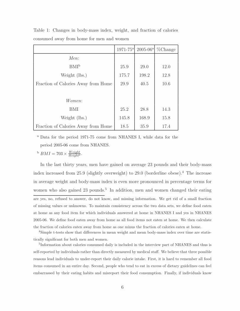
Table 1: Changes in body-mass index, weight, and fraction of calories

consumed away from home for men and women

1971-75a 2005-06a %Change

Men:

BMIb 25.9 29.0 12.0

Weight (lbs.) 175.7 198.2 12.8

Fraction of Calories Away from Home 29.9 40.5 10.6

Women:

BMI 25.2 28.8 14.3

Weight (lbs.) 145.8 168.9 15.8

Fraction of Calories Away from Home 18.5 35.9 17.4

a Data for the period 1971-75 come from NHANES I, while data for the

period 2005-06 come from NHANES.

bBMI = 703 × Weight

Height2.

In the last thirty years, men have gained on average 23 pounds and their body-mass

index increased from 25.9 (slightly overweight) to 29.0 (borderline obese).4 The increase

in average weight and body-mass index is even more pronounced in percentage terms for

women who also gained 23 pounds.5 In addition, men and women changed their eating

are yes, no, refused to answer, do not know, and missing information. We get rid of a small fraction

of missing values or unknowns. To maintain consistency across the two data sets, we define food eaten

at home as any food item for which individuals answered at home in NHANES I and yes in NHANES

2005-06. We define food eaten away from home as all food items not eaten at home. We then calculate

the fraction of calories eaten away from home as one minus the fraction of calories eaten at home.4Simple t-tests show that differences in mean weight and mean body-mass index over time are statis-

tically significant for both men and women.5Information about calories consumed daily is included in the interview part of NHANES and thus is

self-reported by individuals rather than directly measured by medical staff. We believe that three possible

reasons lead individuals to under-report their daily calorie intake. First, it is hard to remember all food

items consumed in an entire day. Second, people who tend to eat in excess of dietary guidelines can feel

embarrassed by their eating habits and misreport their food consumption. Finally, if individuals know

6

habits dramatically and ate out more. The fraction of calories away from home increased

by 11 and 17 percentage points for men and women, respectively.

Our goal in this paper is to determine how much of the increase in weight and the

fraction of calories consumed away from home can be accounted for by the decline in the

relative price of food (at home versus away from home) as well as increases in household

real income. To measure changes in food prices, we introduce a new measure which

considers the price per calorie consumed rather than prices of specific food items. We

calculate price per calorie for food consumed away from home, pA,t, and food consumed

at home, pH,t, as the dollar amount spent by households on each food category divided

by the number of calories consumed:

pA,t =αA,tIt

CaloriesA,t

, pH,t =αH,tIt

CaloriesH,t(1)

We calculate the dollar amount spent by households on food as household real disposable

income, It, multiplied by the expenditure share on food consumed away from home αA,t

or at home αH,t. Information about the expenditure share on food away from home

and food at home is obtained from household expenditures data published by the US

Department of Agriculture (USDA). The expenditure for food away from home is equal

to 3.5 and 4.1 percent, respectively, for the periods 1971-75 and 2005-06. The expenditure

for food away from home is equal to 9.9 and 5.7 percent, respectively, for the same

time periods. Information about nominal disposable income comes from the Bureau of

Economic Analysis (BEA) and we use the consumer price index (CPI) published by BLS

to calculate the real disposable income expressed in 2006 dollars. Between 1971 and 2006,

household real disposable income increased by 24 percent, while the per calorie price of

food consumed away from home declined by seventeen percent (see Table 2).

The price per calorie has two significant advantages over traditional food prices. First,

it provides a simple method for aggregating food items in different categories. Second, it

is intuitively appealing as it controls for changes in portion sizes at restaurants (Young

and Nestle, 2002). Note that the relative price of food away from home is always greater

the interview date in advance, they might change their dietary habits and adjust their calories consumed

downward for one day in order to exhibit “good behavior”. As a result, we do not use self-reported data

on calorie intake in our analysis.

7

Table 2: Changes in per calorie food prices and real income

1971-1975 2005-2006 % Change

Relative price (Away/Home) 1.61 1.34 -16.7

Mean Real Income in 2006 $ $59,742 $74,089 24.0

that one, implying that eating out is more costly than eating at home, even after adjusting

for differences in the number of calories. In addition, we looked at changes in food prices

published by the Bureau of Labor Statistics. We find that the price of food consumed

away from home increased by 40 percent from 1971 to 2006. The increase in food prices

away from home is clearly at odds with the observed increase in the fraction of calories

eaten away from home.

Next, we look at changes over time in the body-mass index and the fraction of calories

consumed away from home for men and women in different age groups. Both economic and

physiological considerations suggest that age matter for eating decisions. First, income

typically increases over the life-cycle reaching its peak around age 50 and then decline

at retirement age. If one thinks of calorie consumption as a normal good, variation in

income over the life-cycle imply that the number of calorie demanded should increase

before age 50 and then decline. Second, the relationship between calorie intake and

weight also differs along the life-cycle. As individuals age, the number of calories needed

to maintain a constant weight declines (see a technical report (2002) published by the

Food and Nutrition Board of the Institute of Medicine of the National Academies).

In Figures 1 and 2, we compare the body-mass index of men and women in different

age groups between 1971 and 2006. First, note that body-mass index increases over the

life-cycle for both men and women and for both time periods. Second, the body-mass

index for men and women increased for all age groups between 1971 and 2006. For men,

the largest increase in body-mass index occurs for the age groups 35-44 and 55-64, while

for women the largest increase occurs for the age groups 25-34 and 45-54.

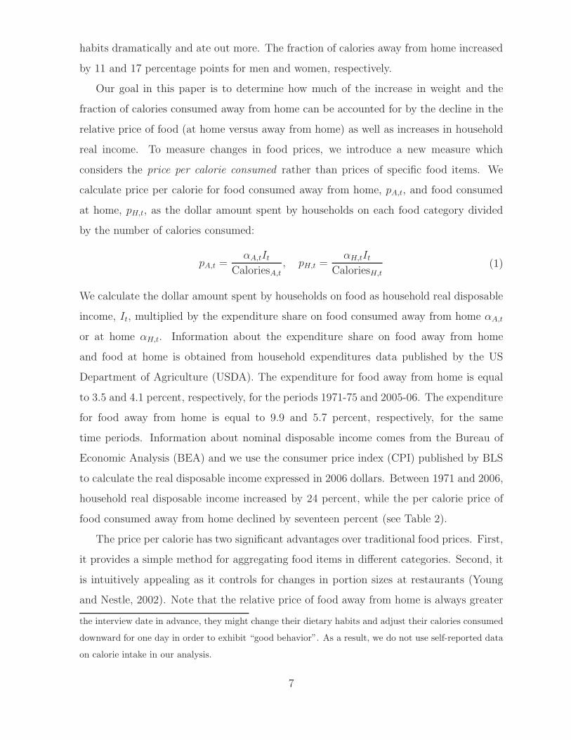
In Figures 3 and 4, we compare the fraction of calories consumed away from home

by men and women in different age groups between 1971 and 2006. First, the fraction of

calories consumed away from home declines with age for both men and women. Second,

8

Figure 1: Men’s body-mass index by age

Figure 2: Women’s body-mass index by age

9

Figure 3: Fraction of calories consumed away from home by men by age

the fraction of calories consumed away from home is greater for men compared to women

for all age groups. Third, the increase in calories consumed away from home between

1971 and 2006 is somewhat uniform for all age group and for men and women.

Finally, we compare household real disposable income for different age group between

1971 and 2006 in Figure 5. First, real income in 2006 is higher than real income in 1971

for all age group. The increase in real income was the largest for the age group 45-54

and the smallest for young adults in age group 25-34. Second, household income follows

a clear pattern over the life-cycle. It increases until age 55 and then declines sharply.

In the next section, we propose a calibrated dynamic model of eating decisions to

assess the quantitative impact of changes in food prices and real income on individual

weight and their decision to eat out.

10

Figure 4: Fraction of calories consumed away from home by women by age

Figure 5: Household real income over time by age

11

3 A Dynamic Optimization Model of Eating Deci-

sions and Weight

Time is discrete and infinite, t = 1, 2, .... In each period, agents decide how much and

where to eat (out or at home) as well as non-food consumption. We let at and ht be the

number of calories consumed away and at home, respectively, and cnft represents non-food

consumption. Calories away and at home are aggregated using a constant elasticity of

substitution (CES) function to obtain food consumption:

cft = (ηa

ρt + (1 − η)hρ

t )1

ρ (2)

with η ∈ (0, 1) and ρ ∈ (−∞, 1]. Food away and at home are perfect substitutes, Cobb-

Douglas, or perfect complements when the parameter ρ is equal to one, zero, or minus

infinity, respectively. The parameter η reflects consumer’s preference for eating at home

or eating out, a smaller η indicating that consumers prefer to eat at home.

Preferences of the representative agent are of constant relative risk aversion (CRRA)

form and are given by:

U(cft , c

nft ) =

[(cft )

α(cnft )1−α]1−σ

1 − σ(3)

with (σ, α) ∈ (0, 1) × (0, 1). The inter-temporal elasticity of substitution between con-

sumption in any two periods is equal to 1σ

and the smaller σ is, the more willing are

households to substitute consumption over time.

Agents make consumption decisions in an environment where their longevity is uncer-

tain. We denote by π(Wt) the conditional probability that a consumer with weight Wt

makes it to the next time period provided that she is alive at the beginning of the period.

We assume that the death probability is an inverted U-shape function of body-mass index

which implies that agents who are either over- or underweight have a greater chance to

die. Finally, death is an absorbing state and consumer receives utility U ≤ 0 forever when

they die.

The expected utility discounted to period one is equal to:

+∞∑

t=1

βt−1Πt−1s=1π(Ws)(π(Wt)U(cf

t , cnft ) + (1 − π(Wt))U) (4)

12

where the parameter β ∈ (0, 1) is the pure time discount factor. Note that it is never

optimal for people to eat so much that they would die with certainty since U(cft , c

nft ) is

positive and U ≤ 0.

The inter-temporal weight law of motion links weight in the next period to current

weight and calorie consumption:

Wt+1 = Wt + λ(at + ht − c(Wt)) (5)

where λ > 0 is a parameter that converts calorie consumption into weight gain and the

function c(Wt) = µ + νWt denotes the daily calorie requirement in order to maintain a

constant weight with ν > 0.

Finally, the budget constraint of the representative agent is given by:

cnft + phtht + patat = It (6)

where we normalized the price of non-food to one, pht and pat are the real price of food

at and away from home, respectively, and agents are endowed with real income It. Note

that a more realistic setting would include credit markets to provide an extra channel

that agents could use to smooth utility over time. The rise in credit availability and use

between 1971 and 2006 might be an important factor for explaining individuals’ decisions

to eat at restaurants (Levy, 2007). In our model, agents smooth utility over time through

the following simple trade-off. Increasing food consumption in the current period yields

instantaneous utility but also leads to higher weight and increased mortality risks in the

future.

For any given sequence of prices and income, {pht, pat, It}t≥1, and an initial weight, W1,

the representative agent chooses an optimal sequence of calories from food away and at

home as well as non-food consumption, {at, ht, cnft }t≥1, to maximize the expected utility

discounted to period one in equation (4) subject to the budget constraint (6), the weight

law of motion (5), the food aggregation equation (2), and non-negativity constraints for

calorie and non-food consumption.

We substitute the weight law of motion into the objective function in equation (4).

The consumption of food away from home, at, and food at home, ht, appear as follows in

13

the objective function:

... + βt−1π(W1) × ... × π(Wt−1)×

(

π(Wt)[(ηa

ρt + (1 − η)hρ

t )αρ (It − phtht − patat)

1−α]1−σ

1 − σ+ (1 − π(Wt))U

)

+

βtπ(W1) × ... × π(Wt)(

π(Wt + λ(at + ht − c(Wt)))[(cf

t+1)α(cnf

t+1)1−α]1−σ

1 − σ+

(1 − π(Wt + λ(at + ht − c(Wt))))U)

+ ...

(7)

We take first-order conditions with respect with food away from home, at, and food

at home, ht. In the Appendix, we show that the system of first-order conditions is given

by:

αηatρ−1

ηatρ + (1 − η)ht

ρ −pat(1 − α)

I − patat − phtht

= −λβ

1 − σπ′(Wt+1)

U(cft+1, c

nft+1) − U

U(cft , c

nft )

α(1 − η)htρ−1

ηatρ + (1 − η)ht

ρ −pht(1 − α)

I − patat − phtht

= −λβ

1 − σπ′(Wt+1)

U(cft+1, c

nft+1) − U

U(cft , c

nft )

(8)

Note that consumer’s utility might not be strictly concave because the survival prob-

ability depends on consumer’s weight. As a result, it is not clear whether first-order

conditions are sufficient for optimality. Although we do not offer a formal proof, we check

in our computer simulations that the allocations that satisfy the first-order conditions in

equation (8) is also utility-maximizing (locally).

We analyze the above system of equations when prices, income, and quantities are

constant over time. That is, when at = a∗, ht = h∗, Wt = W ∗, pat = p∗a, pht = p∗h, and

It = I∗. The weight law of motion in equation (5) provides the relationship between

weight and calorie intake, W ∗ = a∗+h∗−µ

ν. After rearranging slightly, the steady-state

version of the first-order conditions in equation (8) is given by:

ηa∗ρ−1 − (1 − η)h∗ρ−1

ηa∗ρ + (1 − η)h∗ρ =1 − α

α

pa − ph

I∗ − paa∗ − phh∗

αηa∗ρ−1

ηa∗ρ + (1 − η)h∗ρ −pa(1 − α)

I∗ − paa∗ − phh∗= −

λβ

1 − σπ′(

a∗ + h∗ − µ

ν)(1 −

U

U(cf ∗, cnf ∗))

(9)

The steady state food away from home, a∗, and food at home, h∗, are obtained by solving

the above system of equations (9).

14

In the reminder of the paper, we explain our method to calibrate the three key parts

of our model: the weight law of motion, the survival probability function, and the deep

preference parameters. We then use the calibrated model to conduct a lab experiment

where we assess the impact of food price and real income on weight and the fraction of

calories away from home.

4 Calibration

We use medical research on obesity to calibrate the weight law of motion and the survival

probability function. We then chose the remaining preference parameters to match the

average weight and calories away from home for men and women observed in the NHANES

I sample.

4.1 Law of motion

The weight law of motion in equation (5) contains three distinct important parameters.

First, the constant λ converts excess calorie intake into weight gain. Second, the two

parameters (µ, ν) determine the calorie requirement to maintain a constant weight with

c(Wt) = µ + νWt.

According to the dietary guidelines from the US Department of Agriculture, people

gain ten pounds per year if they eat an extra one hundred calories every day above

and beyond the recommended daily calorie intake. As a result, we fix λ = 10100×365

=

2.7397 × 10−4.

According to the Food and Nutrition Board of the Institute of Medicine of the National

Academies (technical report 2002), the minimum number of calories required to maintain

a constant weight depends on gender, age, weight, height, and the activity level. For men,

this daily calorie requirement is given by:

cm = 662 − 9.53 × Age + Activity × (7.23 × Weight + 13.706 × Height) (10)

where age is expressed in years, weight in pounds, height in inches, and the activity level

is equal to 1, 1.12, 1.27, and 1.45, when the activity level is sedentary, low active, active,

and very active, respectively. Note that the number of daily calories required to maintain

15

constant weight declines as men get older but increases with the activity level, weight,

and height. Men’s mean age and height in the NHANES I sample is equal to 41.2 and

69.6 inches, respectively. Assuming a low level of activity (activity=1.12), the calorie

requirement equation for men becomes:

cm(Wt) = 1338.2 + 8.09Wt (11)

The previous equation identifies the parameters µm = 1338.2 and νm = 8.09. For example,

a man of age 41.2 who exercise moderately and weighs 170 pounds needs to eat 2715

calories every day to maintain a constant weight.

For women, the amount of calories needed to maintain a constant weight is given by:

cw = 356 − 6.91 × Age + Activity × (4.25 × Weight + 18.44 × Height) (12)

Women’s mean age and height in the NHANES I sample is equal to 40.3 and 63.6

inches, respectively. Assuming a low level of activity (activity=1.12), the calorie require-

ment equation for women becomes:

cw(Wt) = 1391.1 + 4.76Wt (13)

The previous equation identifies the parameters µw = 1391.1 and νw = 4.76. For example,

a woman of age 40.3 who exercise moderately and weighs 130 pounds needs to eat 2009

calories every day to maintain a constant weight.

In the previous section, we showed that the steady state weight is equal to W ∗ =

a∗+h∗−µ

ν. As a result, the steady state weight for men and women is equal to:

W ∗m =a∗ + h∗ − 1338.2

8.09, W ∗f =

a∗ + h∗ − 1391.1

4.76(14)

4.2 Survival Probability Function

We posit that the survival probability function π(Wt) is given by the following function

form:

π(Wt) = 1 − πa × hr(Wt) (15)

where πa ∈ (0, 1) captures the death likelihood for reasons unrelated to obesity and hr(Wt)

denotes the increased likelihood of death due to being over or underweight. Throughout

16

the rest of the paper, we set πa = 0.01. We use the work of Allison et al. (1999) to

calibrate the hazard rate function hr(Wt). Allison et al. (1999) report the hazard ratios

of death based on six large prospective cohort studies where subjects are placed into two

distinct groups: the control group is comprised of individuals whose body-mass index

(BMI) is between twenty-three and twenty-five; the treated group consists of individuals

with BMI higher than twenty-five. In Table 3, we present their results and it is clear

that the probability of dying tends to increase with BMI. For example, in the Alameda

Country Health Study, people with BMI between thirty and thirty-five have 1.36 more

chance to die compared to people with normal weight, and the hazard ratio increases to

2.79 for people with BMI greater than thirty-five.6

We use the regression algorithm in Judd (1998, p.223) to approximate the hazard rate

function with a linear combination of Chebyshev polynomials, {Ti}ni=0. The algorithm

consists of evaluating a linear combination of Chebyshev polynomials of degree n poly-

nomials at m > n pre-determined nodes on a given weight interval [wmin, wmax]. The

nodes are equal to wk = (zk + 1)(wmax−wmin

2) + wmin for all possible k = 1, ..., m with

zk = −cos(2k−12m

π). In our case, we chose a polynomial of degree six, seven nodes, and we

fix the bounds of the weight interval to correspond to a body-mass index of bmin = 19 and

bmax = 37. Since the seven weight nodes correspond to seven values of the body-mass in-

dex, we use the research by Allison to evaluate the survival probability at all seven weight

nodes with yk = hr(wk).7 Finally, the algorithm provides a formula for the coefficients of

the Chebyshev polynomials with ai =∑k=7

k=1ykTi(zk)

∑k=7

k=1Ti(zk)2

for all possible i = 0, ..., 6. In our case,

the estimated coefficients {ai} are equal to {1.309, 0.302, 0.317, 0.039, 0.064, 0.035, 0.026}.

As a result, the survival probability function is approximated by the following function:

hr(Wt) =i=6∑

i=0

aiTi(2Wt − wmin

wmax − wmin− 1) (16)

for any possible weight in the interval [wmin, wmax]. In Figure 6, we present the survival

probability as a function of the body-mass index. As expected from the Allison’s data,

6Fontaine, Redden, Wang, Westfall, and Allison (2003) calculate years of life lost due to obesity. The

maximum years of life lost for white men twenty to thirty years of age with a severe level of obesity (BMI

> forty-five) is thirteen years and eight for white women.7There is a one-to-one relationship between body weight and body-mass index since BMI = 703 ×

Weight

Height2.

17

Table 3: Hazard Ratios for various BMI categories

BMI Category < 23 [23 - 25) [25 - 26) [26 - 27) [25 - 28) [28 - 29) [29 - 30) [30-35] > 35

Alameda 1.39 1.00 0.98 0.86 1.20 1.26 1.23 1.36 2.79

Framingham 1.12 1.00 0.96 1.11 1.04 1.08 1.41 1.60 1.94

Tecumseh 1.20 1.00 1.18 0.89 1.12 0.92 0.94 1.45 1.87

Cancer Society 1.07 1.00 1.02 1.06 1.08 1.14 1.21 1.35 1.72

Nurses 1.06 1.00 0.92 0.96 1.09 1.21 1.32 1.49 1.89

NHANES 1.04 1.00 0.96 1.11 0.96 1.40 1.06 1.33 1.68

Source: Allison, Fontaine, Manson, Stevens, and VanItallie (1999)

18

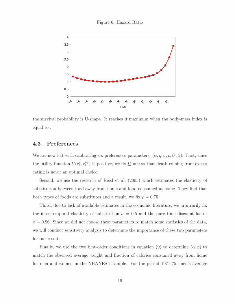
Figure 6: Hazard Ratio

the survival probability is U-shape. It reaches it maximum when the body-mass index is

equal to .

4.3 Preferences

We are now left with calibrating six preferences parameters, (α, η, σ, ρ, U, β). First, since

the utility function U(cft , c

nft ) is positive, we fix U = 0 so that death coming from excess

eating is never an optimal choice.

Second, we use the research of Reed et al. (2005) which estimates the elasticity of

substitution between food away from home and food consumed at home. They find that

both types of foods are substitutes and a result, we fix ρ = 0.75.

Third, due to lack of available estimates in the economic literature, we arbitrarily fix

the inter-temporal elasticity of substitution σ = 0.5 and the pure time discount factor

β = 0.96. Since we did not choose these parameters to match some statistics of the data,

we will conduct sensitivity analysis to determine the importance of these two parameters

for our results.

Finally, we use the two first-order conditions in equation (9) to determine (α, η) to

match the observed average weight and fraction of calories consumed away from home

for men and women in the NHANES I sample. For the period 1971-75, men’s average

19

weight and fraction of calorie consumed away from home was equal 175.7 pounds and

29.9 percent, respectively (see Table 1). According to equation (11), the total number of

calories to maintain a weight of 175.7 pounds is equal to 2760.9, implying that the steady

state value for calories consumed at home and away from home is equal to a∗ = 825.5 and

h∗ = 1935.4, respectively. Per calorie prices of food away from home and food at home

are equal to p∗a = 4.23 × 10−3 and p∗h = 2.97 × 10−3, respectively. Using the information

about real income from Table 2, the steady state of non-food daily consumption is equal

to cnf ∗ = I∗ − paa∗ − phh

∗ = 154.4. As a result, the parameters (α, η) are obtained by

solving the following system of equations:

αη825.5−0.25

η825.50.75 + (1 − η)1935.40.75 −4.23 × 10−3(1 − α)

154.4=

α(1 − η)1935.4−0.25

η825.50.75 + (1 − η)1935.40.75

−2.97 × 10−3(1 − α)

154.4

αη825.5−0.25

η825.50.75 + (1 − η)1935.40.75 −4.23 × 10−3(1 − α)

154.4= −

2.7397 × 10−4 × 0.96

0.5π′(175.7)

(17)

For men, we find that ηm = 0.53 and αm = 0.06.

Finally, we determine the coefficient αw and ηw to match the observed average weight

and fraction of calories consumed away from home for women in the NHANES I sample.

For the period 1971-75, women’s average weight and fraction of calorie consumed away

from home was equal 145.8 pounds and 18.5 percent, respectively (see Table 1). According

to equation (13), the total number of calories to maintain a weight of 145.8 pounds is equal

to 2085, implying that the steady state value for calories consumed at home and away

from home is equal to a∗ = 385.7 and h∗ = 1699.3, respectively. Using the information

about food prices and income from Table 2, the steady state consumption of non-food

is equal to cnf ∗ = 157.0. As a result, the parameters (α, η) are obtained by solving the

20

following system of equations:

αη385.7−0.25

η385.70.75 + (1 − η)1699.30.75 −4.23 × 10−3(1 − α)

157.0=

α(1 − η)1699.3−0.25

η385.70.75 + (1 − η)1699.30.75

−2.97 × 10−3(1 − α)

157.0

αη385.7−0.25

η385.70.75 + (1 − η)1699.30.75 −4.23 × 10−3(1 − α)

157.0= −

2.7397 × 10−4 × 0.96

0.5π′(145.8)

(18)

For women, we find that ηw = 0.49 and αw = 0.04.

Note that men and women differ considerably in their preferences for food versus

non-food goods and food at home versus food away from home. The food share, α, and

the preference parameter for food away from home, η, are greater for men compared to

women. Note that the heterogeneity across gender is not counter-intuitive since men tend

to eat more than women and they also eat more away from home. In the next section, we

use the calibrated model to assess the impact of changes in relative food prices and real

income on eating habits and weight of Americans between 1971 and 2006.

5 Simulations

We perform the following experiments. First, we change the price per calorie of food away

from home from its 1971 value, p1971a = 4.23× 10−3, to its 2006 value, p2006

a = 3.70× 10−3

leaving all other parameters of the model constant. From the first-order conditions in

equation (9), we calculate the new steady state values for food away from home and food at

home. We then calculate the steady-state weight for men and women from equations (11)

and (13), respectively, as well as the resulting body-mass index. We report results of the

first experiment in the first column of Table 4. For men, the fraction of calories away from

home increases by 12 percentage points from 30 percent (calibrated value from Table 1)

to 42 percent. For women, the fraction of calories consumed away from home increases

21

by 8 percentage points from 19 percent (calibrated value) to 27 percent.8 The impact on

agent’s weight is small. Men and women only gain one pound as their weight increases

to 177 and 146 pounds, respectively.

Table 4: Average body-mass index, weight, calorie requirement, and fraction of calories

consumed away from home for men and women

pa ph Income All

Men:

BMI 26 26 28 29

Weight (lbs.) 177 175 194 197

Fraction of Calories Away from Home (%) 42 26 34 36

Women:

BMI 25 25 29 30

Weight (lbs.) 146 144 166 170

Fraction of Calories Away from Home 27 14 21 24

The second experiment consists of changing the price per calorie of food at home from

its 1971 value, p1971h = 2.97× 10−3, to its 2006 value, p2006

h = 2.72× 10−3 leaving all other

parameters constant. We calculate the new steady state value for food away from home

and food at home as well as weight and body-mass index as explained above. We report

the result in the second column of Table 4. For men, the fraction of calories away from

home decreases by 4 percentage points from 30 percent to 26 percent. For women, the

fraction of calories away from home decreases by 5 percentage points from 19 percent to

14 percent. Again, the decline in food prices has little impact on agent’s weight.

The third experiment consists of changing household real disposable income from its

1971 value I1971 = $59, 742 to its 2006 value I2006 = $74, 089 (see Table 2) leaving all other

parameters constant. We report the results in the third column of Table 4. Changes in

8For men, results slightly overshoots the data as the observed fraction of calories consumed away from

home in 2006 is equal 41 percent. For women, results do not fully account for the observed change in the

data as the fraction of calories consumed away from home by women in 2006 is equal to 36 percent.

22

income account for a large fraction of the observed change in individual’s weight. The

steady state weight of men and women increases to 194 and 166 pounds, respectively.9

Changes in income also induce a reallocation effect. As agents become richer, the fraction

of calories consumed away from home increase from 30 percent to 36 percent for men and

from 19 percent to 24 percent for women.

Finally, the fourth experiment consists of changing food prices and income all at once.

For men, the model predicts that a weight equal to 197 pounds and the fraction of calories

away from home is equal to 36 percent. For women, the model predicts that a weight

equal to 170 pounds and the fraction of calories away from home is equal to 24 percent.

The lessons learned from the model for eating decisions and weight can be summarized

as follows. Changes in food prices have an “allocation” effect. As the price of one food

category changes, households substitute from one food category to another. Between

1971 and 2006, the decline in the relative price of food (away from home versus at home)

account for about half of the increase in the fraction of calories eaten away from home.

Changes in food prices, however, have little impact on total calories consumed and weight.

Changes in income, on the other hand, have a large impact on weight. Between 1971 and

2006, much of the increase in weight and body-mass index can be accounted for by increase

in household real disposable income.10

Next, we look at the model predictions for men and women in different age groups. We

allow the preference parameters η and α to differ by age and gender and we re-calibrate

the model as follows. First, we denote by W (g, i) the average weight for men and women

g ∈ {m, f} in age group i ∈ {25−34, 35−44, 45−54, 55−64} observed in NHANES 1971-

75. From equation (11) and equation (13), we calculate the total number of calories for

men and women in each age group to maintain a constant weight. Second, we determine

the number of calories consumed away from home as well as calories consumed at home

9In the data, the mean weight of men and women in 2006 is equal to 198 and 169 pounds, respectively

(see Table 1).10Dolar (2009) shows that the positive relationship between body-mass index and household income

holds for men in several cross-sections of NHANES. For women, however, body-mass index is negatively

related to household income suggesting that some other force not captured in our model is at work.

We leave the task of reconciling the pattern differences for body-mass index and household income in

cross-section and time-series data for men and women for future research.

23

by gender, a(g, i) and h(g, i), respectively as total calories times the fraction of calories

eaten at each location. Finally, the parameters (α(g, i), η(g, i)) are obtained by solving

the following system of equations:

α(g, i)η(g, i)a(g, i)−0.25

η(g, i)a(g, i)0.75 + (1 − η(g, i))h(g, i)0.75−

4.23 × 10−3(1 − α(g, i))

I(i) − paa(g, i) − phh(g, i)=

α(g, i)(1− η(g, i))h(g, i)−0.25

η(g, i)a(g, i)0.75 + (1 − η(g, i))h(g, i)0.75−

2.97 × 10−3(1 − α(g, i))

I(i) − paa(g, i) − phh(g, i)

α(g, i)η(g, i)a(g, i)−0.25

η(g, i)a(g, i)0.75 + (1 − η(g, i))h(g, i)0.75−

4.23 × 10−3(1 − α(g, i))

I(i) − paa(g, i) − phh(g, i)=

−2.7397 × 10−4 × 0.96

0.5π′(W (g, i))

(19)

where information about household real disposable income at age i, I(i), is obtained in

Figure 5. Calibrated values for η and α are reported in Table 5.

Table 5: Preferences Parameters η and α by age and gender

η α

Men Women Men Women

Age 25-34 0.55 0.50 0.07 0.05

Age 35-44 0.54 0.49 0.06 0.04

Age 45-54 0.51 0.48 0.05 0.04

Age 55-64 0.50 0.46 0.06 0.04

The parameters η and α differ considerably by age and gender. First, the food away

from home share, η, is always higher for men compared to women for all age groups and

decreases with age for both men and women. Second, the food share parameter, α, is

greater for men compared to women and also declines with age for men.

In the fifth experiment, we assess the impact of decline in food prices and increase in

real income (altogether) for men and women in the age group 25-34. In the first-order

condition in equation (9), household income I is equal to household real disposable income

24

for the age group 25-34 in 2006 value I200625−34 = $59, 609 (see Figure 5). Per calorie prices for

food away from home and food at home are equal to their 2006 values, p2006a = 3.70×10−3

and p2006h = 2.72 × 10−3, respectively. Finally, the parameters (η, α) are equal to their

calibrated values in Table 5 for men and women. That is, η(m, 25 − 34) = 0.55 and

α(m, 25 − 34) = 0.07 for men and η(m, 25 − 34) = 0.50 and α(m, 25 − 34) = 0.05 for

women.

We solve for the steady state value for food away from home and food at home for

men and women in the age group 25-34. We calculate the fraction of calories away from

home as calories away from home divided by total calories. Finally, from equations (10)

and (12), we calculate the steady state weight for men and women with mean age equal

to 30. We perform similar experiments for men and women for the remaining age groups

from 35-44 to 55-64. We report the results of this experiment for body-mass index and

the fraction of calories away from home for men and women in Figures 7 to 10.

For men, changes in food prices and household income account for a large fraction of

the increase in body-mass index (all of the increase for age group 25-34 and 55-64 and

about 50 percent for age groups 35-44 and 45-54). It accounts for about 50 percent for

women younger than 55 and overshoots for women in the age group 55-64.

Changes in food prices and household income account for more than 70 percent of the

increase in the calories away from home for women and for men older than 45 and more

than hundred percent for men below age 45.

Our results corroborates the existing knowledge on obesity in the following way. On

the one hand, economists who use empirical models found that the impact of food prices

on weight is small (e.g., Chou et al., 2004, Gelbach et al., 2007, or Chouinard et al., 2007).

Using a fully specified calibrated dynamic model, we also find that changes in food prices

over time account for almost none of the weight gain by Americans in the last thirty years.

On the other hand, researchers in the field of public health (e.g., French, Jeffery, Story,

Breitlow, Baxter, Hannan, and Snyder 2001) design small-scale experiments to show that

even small changes in food prices can have strong local effect on individual’s food choices.

For example, the above-mentioned authors examined the effect of lower prices on sales of

lower fat vending machine snacks in 12 work sites and 12 secondary schools. According to

25

Figure 7: Men’s body-mass index by age

a study, price reductions of ten percent, twenty five percent, and fifty percent on low-fat

snacks in vending machines increase the percentage of low-fat snack sales by nine, thirty

nine, and ninety three percent, respectively. Using our calibrated dynamic model, we also

find that change in food prices affect where people eat (at home or out).

26

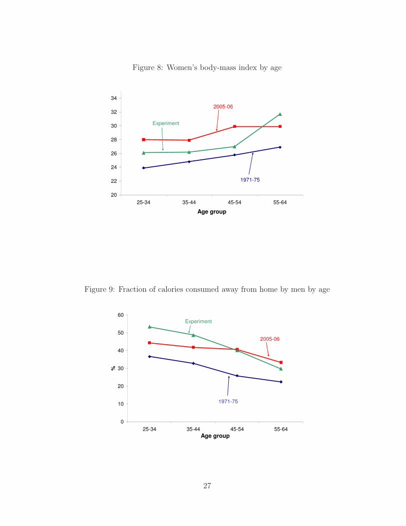
Figure 8: Women’s body-mass index by age

Figure 9: Fraction of calories consumed away from home by men by age

27

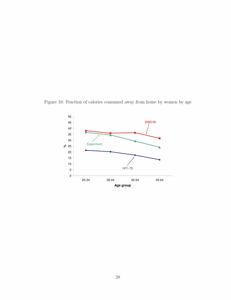
Figure 10: Fraction of calories consumed away from home by women by age

28

6 Concluding Remarks

In this paper, we further analyzed the impact of changes in food prices and household

income on people eating decisions and weight using a dynamic model with rational agents.

After careful calibration of the model using evidence from medical research on obesity,

we found that food prices determine the allocation of calories across food types, while

household income determine the total number of calories consumed and thus individual’s

weight. Between 1971 and 2006, changes in food prices alone account for almost none

of the change in weight of Americans men and women and for more than fifty percent

of the increase in calories consumed away from home. On the other hand, changes in

household income account for more than seventy percent of the increase in men’s and

women’s weight. Because of the limited effect of food price alone on the body-mass index,

we support the view that taxes on food will impact what people eat but will have limited

effect on reducing the population body-mass index or the obesity prevalence.

We see two important avenues for academic research on obesity as well as policy

recommendation. First, educating people about the benefits of eating healthy, exercising

regularly, and the negative health consequences of being obese seem to be promising

policies to win the fight against obesity epidemic. Economic research is needed to measure

the impact of these education programs on individual’s weight and body-mass index.

Second, we derived our results for the impact of food prices on weight and food choices in

an environment where agents are fully rational. An alternative view point is that there

is nothing optimal in being obese and that individuals experience commitment problems

when making food decisions. It is an open and interesting question to revisit the impact

of food prices and household income in a set-up where agents have time-inconsistent

preferences a la Laibson (1997). We leave these two tasks for future research.

29

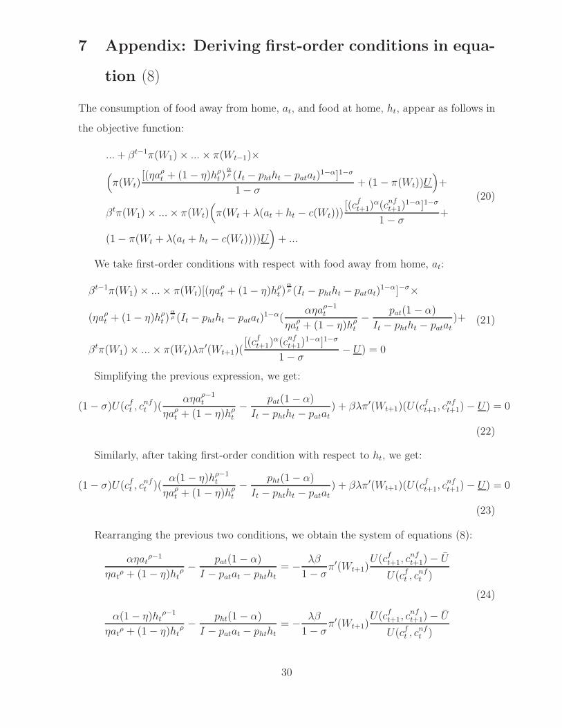
7 Appendix: Deriving first-order conditions in equa-

tion (8)

The consumption of food away from home, at, and food at home, ht, appear as follows in

the objective function:

... + βt−1π(W1) × ... × π(Wt−1)×

(

π(Wt)[(ηa

ρt + (1 − η)hρ

t )αρ (It − phtht − patat)

1−α]1−σ

1 − σ+ (1 − π(Wt))U

)

+

βtπ(W1) × ... × π(Wt)(

π(Wt + λ(at + ht − c(Wt)))[(cf

t+1)α(cnf

t+1)1−α]1−σ

1 − σ+

(1 − π(Wt + λ(at + ht − c(Wt))))U)

+ ...

(20)

We take first-order conditions with respect with food away from home, at:

βt−1π(W1) × ... × π(Wt)[(ηaρt + (1 − η)hρ

t )αρ (It − phtht − patat)

1−α]−σ×

(ηaρt + (1 − η)hρ

t )αρ (It − phtht − patat)

1−α(αηa

ρ−1t

ηaρt + (1 − η)hρ

t

−pat(1 − α)

It − phtht − patat

)+

βtπ(W1) × ... × π(Wt)λπ′(Wt+1)([(cf

t+1)α(cnf

t+1)1−α]1−σ

1 − σ− U) = 0

(21)

Simplifying the previous expression, we get:

(1 − σ)U(cft , c

nft )(

αηaρ−1t

ηaρt + (1 − η)hρ

t

−pat(1 − α)

It − phtht − patat

) + βλπ′(Wt+1)(U(cft+1, c

nft+1) − U) = 0

(22)

Similarly, after taking first-order condition with respect to ht, we get:

(1 − σ)U(cft , c

nft )(

α(1 − η)hρ−1t

ηaρt + (1 − η)hρ

t

−pht(1 − α)

It − phtht − patat

) + βλπ′(Wt+1)(U(cft+1, c

nft+1) − U) = 0

(23)

Rearranging the previous two conditions, we obtain the system of equations (8):

αηatρ−1

ηatρ + (1 − η)ht

ρ −pat(1 − α)

I − patat − phtht

= −λβ

1 − σπ′(Wt+1)

U(cft+1, c

nft+1) − U

U(cft , c

nft )

α(1 − η)htρ−1

ηatρ + (1 − η)ht

ρ −pht(1 − α)

I − patat − phtht

= −λβ

1 − σπ′(Wt+1)

U(cft+1, c

nft+1) − U

U(cft , c

nft )

(24)

30

References

[1] D. Allison, K. Fontaine, J. Manson, J. Stevens, and T. VanItallie. Annual deaths

attributable to obesity in the Unites States. The Journal of the American Medical

Association, 282(16):1530–1538, October 1999.

[2] S. Chou, M. Grossman, and H. Saffer. An economic analysis of adult obesity: results

from the behavioral risk factor surveillance system. Journal of Health Economics,

23(3):565–587, 2004.

[3] H. Chouinard, D. Davis, J. LaFrance, and J. Perloff. Fat taxes: Big money for small

change. Forum for Health Economics and Policy, 10(2), 2007.

[4] V. Dolar. Who is eating away from home? Analysis using NHANES data 1971-2006.

Working Paper, October 2009.

[5] K. Fontaine, D. Redden, C. Wang, A. Westfall, and D. Allison. Years of life lost

due to obesity. The Journal of the American Medical Association, 289(2):187–193,

January 2003.

[6] Food and Nutrition Board. Dietary reference intakes for energy, carbohydrate, fiber,

fat, fatty acids, cholesterol, protein and amino acids. Technical report, Institute of

Medicine of the National Academies, Washington D.C. - National Academy Press,

2002.

[7] S. French, R. Jeffery, M. Story, K. Breitlow, J. Baxter, P. Hannan, and P. Snyder.

Pricing and promotion effects on low fat vending snack purchases: the chips study.

American Journal of Public Health, 91(1):112–117, January 2001.

[8] J. Gelbach, J. Klick, and T. Stratmann. Cheap donuts and expensive broccoli: the

effect of relative prices on obesity. March 2007.

[9] K. Judd. Numerical Methods in Economics. MIT Press, 1998.

[10] D. Laibson. Golden eggs and hyperbolic discounting. Quarterly Journal of Eco-

nomics, 62, May, pp. 443-77, 62:443–77, May 1997.

31

[11] A. Levy. A theoretical analysis of rational diet of healthy and junk foods. Economics

Working Paper 07-01, University of Wollongong, 2007.

[12] L. Powell and F. Chaloupka. Food prices and obesity: Evidence and policy implica-

tions for taxes and subsidies. The Milbank Quarterly, 87(1):229–257, 2009.

[13] A. J. Reed, W. Levedahl, and C. Hallahan. The generalized composite commodity

theorem and food demand elasticity. American Journal of Agricultural Economics,

87(1):28–37, February 2005.

[14] L. Young and M. Nestle. The contribution of expanding portion sizes to the US

obesity epidemic. American Journal of Public Health, 92(2):246–249, February 2002.

32