a simple notation for differential vector expressions in orthogonal

Geophys. J . Int. (1993) 115, 654-666

A simple notation for differential vector expressions in orthogonal curvilinear coordinates

Edward W. Bolton Department of Geology und Geophysics, Yule Universiry, Kline Geology Laboratory, PO Box 6666, New Haven, CT 06511-8130, USA

Accepted 1993 March 21. Received 1993 March 19; in original form 1992 October 23

S U M M A R Y We present a simple notation for performing differential vector operations in orthogonal curvilinear coordinates, and for easily obtaining partial differential expressions in terms of the physical components. We express nth-order tensors as the summed products of the physical components and nth-order polyads of unit vectors (an extension of Gibbs dyadic notation convenient for a summation convention). By defining a gradient operator with partial derivatives balanced by the inverse scale factors, differential vector (or tensor) operations in orthogonal coordinates do not require the covariant/contravariant notation. Our primary focus is on spherical-polar coordinates, but we also derive formulae which may be applied to arbitrary orthogonal coordinate systems. The simpler case of cylindrical-polar coordinates is briefly discussed. We also offer a compact form for the gradient and divergence of general second-order tensors in orthogonal curvilinear coordinates, which are generally unavailable in standard handbooks. We show how our notation relates to that of tensor analysis/differentiaI geometry. As the analysis is not restricted to Euclidean geometry, our notation may be extended to Riemannian surfaces, such as spherical surfaces, so long as an orthogonal coordinate system is utilized. We discuss the Navier-Stokes equation for the case of spatially variable viscosity coefficients.

Key words: differential geometry, fluid dynamics, numerical modelling applications, orthogonal coordinates, spherical coordinates.

1 INTRODUCTION

Spherical, cylindrical, and other more complex geometries occur in numerous scientific applications. The primary reason for adopting curvilinear coordinates arises from the simplification of boundary conditions when the problem is expressed in its natural geometry. The use of spherical coordinates is the logical choice for many problems in planetary and stellar dynamics. The differential vector operations implicit in the governing dynamical equations, when translated into curvilinear coordinates, produce new terms due to the spatial dependence of the basis unit vectors. Despite the variety of means for dealing with this problem, a practical formulation applicable to general cases in orthogonal coordinates remains generally inaccessible to those without training in differential geometry or tensor analysis. Our notation, being similar to that in use for rectangular coordinates, enables those who have training in vector calculus to derive partial differential expressions for the physical components of general differential vector and

tensor operations, so long as an orthogonal coordinate system is adopted.

Although non-orthogonal coordinates are occasionally adopted, orthogonal coordinate systems are in common use for theoretical, numerical and other applications. In addition to the simplification of the boundary conditions, the wealth of theory for orthogonal expansion functions often motivates the choice of an orthogonal coordinate system. Numerical modelling in spherical geometries, typically formulated in orthogonal coordinates, plays an important role in geophysics. As more complex phenomena are investigated, easily derived general formulae for differential vector operations should prove useful.

Differential geometry provides an efficient way for dealing with complexities such as non-orthogonal coordinates, topologically curved space, and the space-time coordinates of relativity. In that description, Euclidean space is ‘flat’, even when it is described by curvilinear coordinates. The most general approach, however, often carries unnecessary ‘baggage’ for the practitioner desiring an understanding of

Dow

nloaded from https://academ

ic.oup.com/gji/article-abstract/115/3/654/608796 by guest on 09 April 2019

Differential vector operations 655

vector operations in orthogonal curvilinear coordinates. Although results obtained by using the notation presented here may be derived by other means, we have found our notation more compact and physically motivated. The surface of a sphere is non-Euclidean, for which analysis involves Riemannian geometry. Although we focus on 3-D Euclidean space, our analysis is not restricted to Euclidean space. Therefore, the notational simplifications for orthogonal coordinates, which we attempt to exploit fully, may be extended to Riemannian surfaces, such as a spherical surface described by spherical coordinates (cf. Section 7 and Backus 1967).

The notation developed here should prove to be convenient for continuum mechanics and electrodynamics in any orthogonal curvilinear coordinate system. In geophysics, numerical modelling of fluid flows in thick spherical shells (e.g. mantle and outer core flows), is being pursued with increasing vigor. We were motivated t o find a simple notation by the problem of thermal convection in spherical shells with temperature-dependent viscosity, for which the viscous term in the Navier-Stokes equation may take an unusual form. We discovered a compact way of dealing with differential vector operations in orthogonal coordinates.

By restricting the analysis to orthogonal coordinates, and by defining a ‘balanced’ gradient operator, we may consistently transform coordinate-free, differential vector equations directly into equations for the physical components, avoiding the covariant/contravariant notation entirely. Truesdell (1953) presents formulae for obtaining the physical components of vectors and tensors from their covariant and/or contravariant forms. By contrast, we emphasize the direct conversion of coordinate-free notation into physical-component form. Although Truesdell con- siders both orthogonal and non-orthogonal coordinate systems, we restrict our development to orthogonal coordinates. Happel & Brenner (1986) present a method somewhat similar to ours, but they d o not take advantage of a summation convention, nor the convenience of transformation matrices. (Their monograph includes two very useful appendices on orthogonal coordinates and tensor operations.)

Our notation for orthogonal curvilinear coordinates is proposed as a simple alternative to the covariant/ contravariant notation (cf. Morse & Feshbach 1953, Chapter l ) , differential forms, and other standard differential formulae derived from limits of integrals (e.g. Morse & Feshbach 1953, Chapter 1; and Arfken 1970, Chapter 2). The convenience of a summation convention, and the introduction of differential transformation matrices, facilit- ate the ‘bookkeeping’ necessary to derive explicit forms of the commonly used differential vector operations, and other forms less commonly used.

The formulation presented here for orthogonal coordinates is more efficient for translating coordinate-free notation into component form than methods which use the Christoffel symbols, because our transformation matrices take advantage of some cancellation. We shall provide specific examples for Euclidean space described by spherical-polar coordinates, and provide the tools necessary for general orthogonal coordinates. The case of cylindrical- polar coordinates is particularly simple. The notation is of course also applicable t o rectangular coordinates, but its

utility is specifically for orthogonal curvilinear coordinates, where the orientation of the unit vectors is spatially dependent and notational extensions from the rectangular system are required. We also believe that our notation is correct even in non-orthogonal coordinate systems, although the transformation matrices we introduce would lack their sparse character, and dot products of unit vectors would no longer produce the Kroneker delta.

We first develop the notation in spherical-polar coordinates in Section 2, pedagogically illustrating its usage and utility by performing the common operations of vector calculus. In the process, we derive general formulae applicable to arbitrary orthogonal coordinate systems. The basic tools necessary for derivations in cylindrical coordinates are given in Section 3, along with a simple example. In Section 4, we develop notation for tensor products, and a compact form for the gradient and divergence of general second-order tensors. These latter results are unavailable in most standard mathematical handbooks. In Section 5, we show how our notation relates to traditional tensor analysis and differential geometry. In Section 6 we discuss the Navier-Stokes equation in curvilinear coordinates, and a useful vector identity. In Section 7 we develop compact expressions for the surface gradient and divergence of tangent tensor fields. Concluding remarks are made in Section 8.

2 FORMULATION FOR SPHERICAL- POLAR COORDINATES WITH GENERAL FORMULAE FOR ARBITRARY ORTHOGONAL C O O R D I N A T E SYSTEMS

In spherical-polar coordinates, position is represented by the triplet 4 = ( E l , Ez, 5,) = [ r , 8, $1, representing the radial, colatitudinal and (eastward) azimuthal magnitudes. The transformations between spherical and rectangular coordinates are as defined in Table 1.

We adopt the corresponding ord_er for the unit vectors: {Sl, S 2 , &} = {i, 8, $}, where i, 8, and $ are the unit vectors in the directions of increasing r, 8, and $, respectively. Indices will always be located as subscripts to the right of the variables t o which they refer. The orientation of unit vectors depends upon the position 6. For applications to other orthogonal coordinate systems, the order of unit vectors should be such that the system is right handed, with 2, = k1 x S2. The order of coordinates for the position and unit vectors should conform to this choice in a way analogous to the above choice for spherical-polar coordinates.

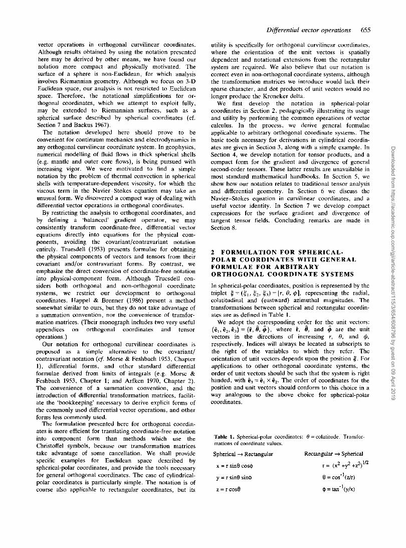
Table 1. Spherical-polar coordinates: 8 = colatitude. Transfor- mations of coordinate values.

Spherical -+ Rectangular Rectangular + Spherical

x = r sine COSQ, r = (x2 +y 2 +z 2 ) If2

y = r sine sin@ e = C O S - ~ W )

Q, = tan-l(y/x) z = r cost3

Dow



656 E. W. Bolton

2.1 Vectors and tensors

We shall explicitly represent the presence of unit vectors in all vector and tensor quantities. We represent a general vector as a = & , where the summation convention is assumed: repeated (dmmy) indices are to be summed over their range (1,2,3). Thus, a = a$, = a,C, + a,2, + a& = a,i + aH6 + a+4 (the latter specialized for spherical-polar coordinates). The vector components, a,, are assumed to be well-behaved functions of space and time. Tensors will be represented by T = T,ki?,&. For non-symmetric tensors, T k i , 6 k # Tki ik6 , , so the order of placement of the unit vectors is important. The placement of the components of the tensor is arbitrary, so that T,kiiii?k = @,T,,@, = &,C,T,,. This is Gibbs’ dyadic notation (Gibbs & Wilson 1925), but applied to curvilinear coordinates, and put in a form convenient for a summation convention. As a specific example in spherical-polar coordinates, the tensor component cH is simply T,,, and it is the component which multiplies GI&, = i8 in the above notation. The components, a, and T k r are called ‘physical components’ in most tensor analysis and differential geometry texts. In Sections 5-7, they will be denoted a(i) and T(ik) .

2.2 Dot products and cross products

Dot products of unit vectors take their usual form, ei - & = 6 ; k ; where 6, is the Kronecker delta symbol: Sik = 1 for i = k, 6, = 0 for i # k. The cross product of the unit vectors, for right-handed coordinate systems, is 6; X kk = where Emjk is the permutation, Levi- Civita, or alternating symbol: Em;k = 1 for rn, i, k being cyclic permutations of 1, 2, 3; &,;k = -1 for cyclic permutations of 2, 1, 3; and &-;k = 0 if any of the indices are equal.

The dot product of vectors is then (assuming the summation convention):

23 * b = a,&; a b$k = U;bk&i * 6, = U j b k 6 j k = sib;.

X b k 6 k = U;bki?i X ek = aibkem&mik

(1)

(2)

The cross product of vectors is

a X b =

where there is an implied sum on i, k and rn in the last term.

2.3 Gradient of scalars

We define the usual scale factors (cf. Morse & Feshbach 1953) for spherical-polar coordinates: (h i , h,, h,) = (1, r, r sin 8). Note that the ith scale factor is independent of the ith coordinate for spherical coordinates. We find it convenient to define the inverse of the scale factors: Pj = l/hi. (Although our notational choice of hi conforms to the most common usage, some authors use hi for our symbol P;, e.g. Edwards, Brenner & Wasan 1991.) For rectangular coordinates, all the scale factors are 1. Partial differential

a d d operators will be denoted (a,, d,, a,)( = [- - -1

dr‘ 38’ 36 for spherical-polar coordinates), or by comma notation defined below. The above notation is summarized in Table 2.

Table 2. Summary of notation for spherical polar coordinates.

i ti ai hi Pi ei -

1 r a, 1 1 e 2 e ae r 4 r 1 -

3 Q r sine a, 1 -

r sine 4 The gradient operator takes the form:

v = &npn 3,. (3) Again, a summation convention is assumed, but we now allow three repeated indices when the factor P,, is present, so that V = 2iP1 d, + C,P, d, + C,P, d,. When the gradient operator acts upon vectors or tensors, we must distinguish between V, and V, as discussed below. The gradient of a scalar reduces to the usual form:

VlY = CnPn dnW (4a)

where we have used comma notation for partial derivatives

(e.g. q,l = q.r =:). Note that q., is really a covariant

partial derivative of a scalar, but comma notation is defined differently in Section 5. The form for the gradient of a scalar in eq. (4a) is applicable to all orthogonal coordinate systems, whereas this is specialized for spherical-polar coordinates in eq. (4b).

2.4 Gradient of vectors

The unique feature of differentiating vectors in curvilinear coordinates is that both the vector components and the unit vector orientations are generally functions of space. By the product rule, dn(a) = dn(al4ii) = u , , ~ C , + The properties of d,(&) = 6i,n are such that & I Ci and & is also a unit vector, which may have components in both directions orthogonal to 6;. This orthogonality property, (GiJ - C; = 0, of unit vectors in orthogonal curvilinear coordinates is not generally shared by the covariant basis vectors discussed in Section 5.

We may conveniently represent the directional changes arising from partial differentiation of unit vectors by introducing a transformation matrix. We write:

&, = d,(C,) = Anik@k ( 5 )

where there is an implied sum on k. By defining this transformation of unit vectors, summing on repeated indices, and by defining a balanced gradient operator, we avoid the need of covariant and contravariant quantities and the Christoffel symbols (this is discussed in Section 5). Of the 27 components of Anik, only six are non-zero for spherical-polar coordinates, namely:

A,,, = 1, A,,, = -1, A,,, = sin 8,

A3,, = cos 8, (6)

A,,, = -sin 8, A,,, = -cos 8.

Dow




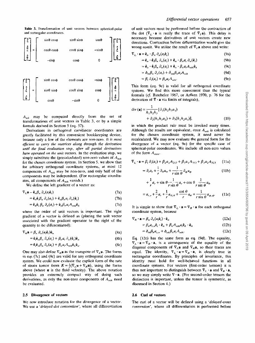
Table 3. Transformation of unit vectors between spherical-polar and rectangular coordinates.

A,, may be computed directly from the set of transformations of unit vectors in Table 3, or by a simple formula derived in Section 5 (eq. 57).

Derivations in orthogonal curvilinear coordinates are greatly facilitated by this convenient bookkeeping device, because only a few of the elements are non-zero. I t is most efficient to carry the matrices along through the derivation until the final evaluation step, after all partial derivatives have operated on the unit vectors. In the evaluation step, we simply substitute the (precalculated) non-zero values of AIllk for the chosen coordinate system. In Section 5, we show that for arbitrary orthogonal coordinate systems, at most 12 components of A,, may be non-zero, and only half of the components may be independent. (For rectangular coordinates, all components of Anik vanish.)

We define the left gradient of a vector as:

where the order of unit vectors is important. The right gradient of a vector is defined as (placing the unit vector associated with the gradient operator to the right of the quantity to be differentiated):

',a = P n an(a$,)6n

= CAP" a"@,) + P,a, ~,,(W" (8b)

= cicnfin + PnarAntk6k6n. (8c)

One may also define V,a as the transpose of V,a. The forms in eqs (7c) and (&) are valid for any orthogonal coordinate system. We could now evaluate the explicit form of the rate of strain tensor from E = i(V,u + V,u), using the forms above (where u is the fluid velocity). The above notation provides an extremely compact way of doing such derivations, as only the non-zero components of Anrk need be evaluated.

2.5 Divergence of vectors

We now introduce notation for the divergence of a vector. We use a 'delayed-dot convention', where all differentiation

of unit vectors must be performed before the contraction of the dot (V,-a is really the trace of V,a). This delay is necessary because derivatives of unit vectors create new directions. Contraction before differentiation would give the wrong result. We utilize the result of V,a above and write:

This form (eq. 9e) is valid for all orthogonal coordinate systems. We find this more convenient than the typical formula (cf. Batchelor 1967, or Arfken 1970, p. 76 for the derivation of V * a via limits of integrals),

+ I h3aJ + W I hza,)l, (10)

in which the product rule must be invoked many times. Although the results are equivalent, once Anik is calculated for the chosen coordinate system, it need never be recalculated. We may now evaluate the general form for the divergence of a vector (eq. 9e) for the specific case of spherical-polar coordinates. We include all non-zero values of the form Amin.

V L . a = P i di(ai) + pza,A, , , + P3aIA313 + P3aZA323 (Ila) 1 1

= drar + - 3,a, + ~

r r sin 8 %a,

1 1 1 +-a,+sin 0- a, + cos 8-

r r sin 8 r sin o a*

2 1 cot 0 1 (11c) - - ar.r + -a, + - a , , + __a,, + - r r r r sin e a**w

It is simple to show that V, - a = V, * a for each orthogonal coordinate system, because

V, - a = f?, 3,(aiEi) - 6, (12a)

(12b)

( 12c)

- - P,,aj,,&; * 6, + @,Anjkai6k ' 3,

= GniPna,.n + snk@naiAnik.

Eq. (12c) has the same form as eq. (9d). The equality, V L - a = V , - a , is a consequence of the equality of the diagonal components of V,a and V,a, so their traces are equal. The identity, V,-a=V, - a , is clearly true in rectangular coordinates. By principles of invariance, this identity must hold for well-behaved functions in all coordinate systems. For vectors (first-order tensors) it is thus not important to distinguish between V, * a and V, - a, so we may simply write V - a. (For second-order tensors the distinction is important, unless the tensor is symmetric, as discussed in Section 4.)

2.6 Curl of vectors

The curl of a vector will be defined using a 'delayed-cross convention', where all differentiation is performed before

Dow



658 E. W. Bolton

the unit vectors are crossed. So, we define:

V L x a = 6, x P, a,(a,@,) (13a)

(13b)

( 13c)

= C,c x CiP,,ui,, + 6, x P,aiAnikCk

= CmEmniP,rai.n + CmEmnkPnaiAnik .

The form in eq. (13c) is valid for all orthogonal coordinate systems. We now specialize this for spherical-polar coordinates. Note that E ~ ~ ~ A , ~ ~ may be simplified by writing the non-zero components of Anik, thus

&mnkAnik = K 2 2 A 2 1 2 + &m2IA22l + K 3 3 A 3 1 3

+j9&3nA323 + &m31A331 + Em32A332 ( 14)

where we have placed crosses on vanishing components of the permutation symbol. After substituting Pn, ui and the A's in the above, the usual form for V X a in spherical-polar coordinates is immediately recovered. We also choose to define V , x a = P, dn(a,Ci) x C,, which after evaluation yields the negative of V , X a.

2.7 Laplacian of a scalar

The Laplacian of a scalar may be defined as:

"11, = v L . ( v L q > = ' P n an(ckPk ' k q ) . (15) In this expression, the product rule will give rise to three terms. Before proceeding, it is convenient to define

Bnk (16)

Of the nine components of B,,k, only three do not vanish for spherical-polar coordinates, namely:

The fact that the diagonal elements of B,, vanish will imply that the d,,Pk type terms in the Laplacian of a scalar will also vanish after the contractive dot is performed. This is true for spherical-polar and cylindrical coordinates, but is not true in general. We now expand V 2 q .

v2v = Cn * P n ( A n k m C r n P k q , k + C k B r z k q , k + C k P k q , k n ) (18a) = P n ( A n k n P k v. k + B n ~ q . n + 6, q , n n ) . (18b)

The form in eq. (18b) is valid for any orthogonal coordinate system. This form may be contrasted with

of Arfken (1970) or Batchelor (1967), where the product and quotient rules must be invoked many times. For the case of spherical-polar coordinates, we include only the non-zero elements, thus:

V2W = P2PIA212V.I+ P3PIA313W.I

+ PRP2A323W.2 + a:w.1 I + m . 2 2 + p : w . 3 3 . (20)

Upon evaluating the 0's and A's, the usual expression for V 2 w is recovered.

2.8 Laplacian of a vector

The most tedious derivation we consider here is the Laplacian of a vector, which may be viewed as the contraction of a third-order tensor. Most authors (e.g. Batchelor 1967, p. 600) choose to evaluate V2a via the vector identity

V2a = V(V - a) - V x (V x a ) (21)

but we shall compute it directly, for the pedagogical illustration of our notation which uses a single definition of the gradient operator. In curvilinear coordinates, the Laplacian of a vector is more complicated than the Laplacian of a scalar due to the spatial dependence of the unit vectors. To highlight this difference, some authors have chosen a special symbol. For the case of the Laplacian of a vector, Moon & Spencer (1961) use the operator symbol @. Contrary to their remarks, one may still define V 2 as V . V , so long as contraction follows all differentiation of unit vectors. Before proceeding, it is convenient to define:

We summarize the important features of our notation in Table 4.

Of the 81 components of Cnkim, only four do not vanish for spherical-polar coordinates. They are:

c23,, = cos 8,

C,,,, = -COS 8,

C,,,, = -sin 8,

C,,,, = sin 8.

The Laplacian of a vector will involve a term of the form Cnnim, which vanishes for spherical-polar coordinates. The details of the derivation of V2a are shown below. The order of the unit vectors is important, and the dot is understood to act between 'adjacent' unit vectors. Extensions of this rule are discussed in Section 4.

Table 4. Important definitions and conventions (summation on repeated indices).

Dow




where we have renamed indices going from eq. (24e) to (24f). The form for V2a in eq. (24f) is valid for all orthogonal coordinates. Now, for spherical-polar and cylindrical coordinates, the terms Bnn and Cnnim vanish, so that:

VZa = k ( A n k n P n P k a . v . k + Pfias,nn + AnknPn@kaiAkb

+ 2P2,ai.nAniT + PZnaiAninPnms) . (25)

The leading two terms on the right-hand side have the form of V2 acting on the physical components of a, as can be seen by comparing to V'V of eq. (18b). These two leading terms yield:

iv2u, + 8V2U" + @u,. (26)

We now specialize the remaining terms of eq. (25) for spherical-polar coordinates. The non-zero components of 2&j,nA,,k6s yield:

2P:a I , 2 A 2 1262 + 2 P % 2 . ~ 4 2 2 1 6 I + 2 P : a i . 3 A 3 136.1

+ 2 P : a 2 . 3 A 3 2 3 6 3 + 2P:a3 .3A3 .3 le l + m % , 3 A 3 3 2 % . (27)

P 3 A 3 2 3 B 2 a IA212C2 + P 3 A 3 2 3 P 2 a 2 A 2 2 1 6 ' ( 28 )

The non-zero components of &&A,timA,pm,s6.y yield:

P & i A 2 i 2 A z 2 1 6 1 + P:azAzz, A 2 1 2 6 2

The non-zero components of A n k n / 3 n P k a i A k h 6 s yield:

+ P : a I A 3 1 3 A 3 3 1 ~ 1 + B : a , A 3 , 3 A 3 3 2 ~ 2

+ P : a 2 A 3 2 3 A 3 3 , & 1 + P:a ,A323A332&2

+ P:a2'4331A313&3 + P : a , A 3 3 2 A 3 2 3 6 3 . (29)

After substituting the values of the P ' s and A's, and collecting terms, the usual expression for V'a in spherical-polar coordinates is recovered. It is simple to show that V, (V,a) = V, - (V,a) = V'a, for vector a. But V, + (V,a) # V, (V,a). In fact, V, - (V,a) = V,(V, * a) = V(V - a) = V,(V, - a) = V, * (V,a). This fact allows simplification of the viscous term of the Navier-Stokes equation for incompressible fluids, and is discussed further in Section 6 .

2.9 The inertial term and the associated 'curvature terms'

The inertial term of the Navier-Stokes equation in an Eulerian frame, [u * (V,u)], leads to the so-called 'curvature

terms'.

The form for u - (V,u) in eq. (30f) is valid for all orthogonal coordinate systems. We now deal with these terms separately for spherical-polar coordinates. The first term in eq. (30f) leads to the usual form of the initial term, while the second leads to the so-called 'curvature terms'. The first term yields:

~ i P ; ~ ~ , i t m = U I P I U m . 1 6 m + ~ 2 P 2 u m . 2 ' m

+ U3P3Um,@m (31a)

+ U , P I 1 1 2 , , & 2 + u 2 P 2 u 2 . 2 5 2 + U 3 P 3 U 2 . 3 ~ 2

+ U l P l ~ 3 . 1 ~ 3 + U2P2U.3.2& + %iP,U3.363

= U I P I U I . I ~ I + u 2 P 2 u 1 . 2 ~ 1 + U 3 P 3 U 1 . 3 ~ I

(31b)

= ?(u - V)U, + 6(u - V)uH + C(U * V)U,. (31d)

We now write down the six non-zero components of UiP;UkA;km6m (the second term of eq. 30f), to yield:

1 + 3 [ uHu@(cos O)]

1 r sin 0

1 r sin 0

u,u,(-sin 0)

+e[- u, u+ (-cos 0)

+ j ( % + W C O t r r 0 ) .

The usual expression for u - (Vu) in spherical-polar coordinates is recovered by combining eqs (31d) and (32b). This concludes our illustration of the usage of this notation as applied to common differential vector operations in spherical-polar coordinates. Additional formulae may be found by evaluating results presented in 4.

Dow



660 E. W. Bolton

3 FORMULATION FOR CYLINDRICAL- POLAR COORDINATES

In cylindrical coordinates, position is identified by s, @, and z : s is the shortest distance from an axis, z is the (signed) distance from the origin along the axis, and @ is an eastward azimuthal angle. We adopt the order = [ E l , E 2 , E3] = [s, @, 21, and {C,, i2, C,} = {3, 6, i } . The scale factors have the form h , = h, = 1, and h, =s. As was the case for spherical-polar coordinates, the ith scale factor is independent of the ith coordinate. As before, we define Pi = l / h i , and 3,(Gi) = AnikCk. For cylindrical coordinates, Anik has only two non-zero components: A, , , = 1 and A,,, = -1. This implies that each of the 81 components of Cnkim vanishes [Cnkim = d n ( A k j m ) ] . Of the nine components of Bnk(=3,Pk), all vanish except for B,, = - l/s2. Except for these differences in component values, all rules of notational usage developed for spherical coordinates are applicable for the cylindrical case, and the general formulae for orthogonal coordinates, given in Section 2, may be evaluated using the non-zero components of the transformation matrices.

The notation presented here also allows efficient translation between representations in different coordinate systems. We offer a sim_ple example. In a rectangular system, let u = ui + u j + wk. Suppose we desire to calculate a,u, but that the data is known only in a cylindrical coordinate system: u = (u,$ + u+$,+ u,k) = uiGi. Now, a,u =i * [i. (V,U)] . But, i = 3 cos @ - IP sin @ = amb,, (with a1 = cos @, a2 = -sin @, a3 = 0, and C, is in the cylindrical system). Then,

?. ..

a,u = i [i + (V,U)]

= a,Gm - {&,Sj [CJ, a,(u,C,)]} = . ' (6nPnUt.nCi + enPnUiAnikCk) l

= amCm * (lY,6jn/?nUi,nei + CY,6,nPnUiAnikek)

= am(a/smip,ui./ + a j6mkpju iAj ik )

= amaj/3Ju,,j + a m a j P i u i A j i , . (33) We now write the non-zero components of the a's and the A's to yield:

a,u = ~ . I ~ I P I U I . I + ' y [email protected] + ~ 2 ~ I P I U 2 . I + a 2 a 2 B 2 u 2 . 2

+ 'Y2(r2P,UIA212 + ~,~2P,u*A, , , . (34) When this is translated using the above definitions, we have:

(35)

This derivation would be considerably more cumbersome using other notations.

4 SECOND-ORDER TENSORS: THEIR GRADIENT, DIVERGENCE A N D GENERAL PRODUCTS

Second-order tensors are commonly encountered in scientific applications, the stress tensor and the velocity gradient tensor being two examples. Suppose T is a general second-order tensor. The gradient of T is a third-order

tensor. The gradient operator acts on the components of the tensor and on both of the ordered unit vectors. The 'left' gradient takes the (triadic) form:

v, T &,P,, d, ( TkjCkCi ) (36a)

(36b) = e,,P,,(Tk;,nek6j + Tki&k,,&i + Tkj&kCi, , , )

= CnPn( Tki ,n&k6j + TkiA,,k,@,&i + Tki&kAnrrn6,,,). ( 3 6 ~ )

Again, the order of placement of the unit vectors is important. From the above, we can immediately evaluate the (left) divergence of a general second-order tensor by contracting the two leading unit vectors.

a = @n(Tki.n6nkCi + Tki6nrnAnkmCi + TkistlkAnim&m)

(37a) (37b)

v.L ' = Pn(Tnm.n + TkmAnkn + TnkAnkm)Crn. (37c)

= Pn(Tni .nCi + TkiAnkn&i + TniAnimCm).

This may be rewritten by changing dummy indices.

For final evaluation of this form, the implied summation on repeated indices is performed, and only the non-zero components of Ankn and Anim for the chosen coordinate system need be considered. Similarly, the right gradient yields:

' R T = P n dri(Tkt#kCi)in (38a)

= Pn( Tki, ,Ck6i + T k i A n k , , , 6 , ~ i + Tki8kAnirnCm)&n. (38b)

We may now calculate the right divergence by contraction of the two trailing unit vectors, which after rearranging, yields:

vR . = P n ( T m n . n + TmkAnkn + TknAnkm)ern. (39) We have been unable to find any means more convenient for evaluating such quantities in curvilinear coordinates. In addition, these forms appear to be unavailable in any mathematical handbook. The divergence of a second-order tensor is part of the viscous term of the Navier-Stokes equation. In that case the second-order tensor is the symmetric rate of strain tensor. Note that V , - T = V , - T only for symmetric T, and that 0, - T = ( V , - transpose ( T ) ) for second-order tensors. Most texts in tensor analysis and differential geometry, which consider these forms, appear to define div ( T ) as V , * T, whereas texts in fluid dynamics commonly use V , . T , as discussed below. By choosing ordered unit vectors, we avoid ambiguities. Rosner (1986) gives a formula for the divergence of a general second-order tensor, expressed in orthogonal coordinates. His formula is for a 'left' divergence. A term analogous to TnkAnkmCm of eq. (37c) should be included in Rosner's eq. (2.5-33). Happel & Brenner (1986, Appendix A) also give an explicit formula for the left divergence of a general second-order tensor. Their approach is quite similar to ours, although they do not take advantage of a summation convention, nor the transformation matrices. (Note that hi of Happel & Brenner is equivalent to our Pi = l / h i . ) Aki & Richards (1980, Vol. 1, eq. 2.48) give an explicit formula for the first component of the divergence of a second-order tensor. Their formula is not easily extended for the remaining two components, and is correct only for symmetric tensors. [The correction for non-symmetric tensors is as follows: upon the replacement of r3' by t', their formula would be correct for 6, * (V, - T ) . Alternately, upon the replacement of t" by

Dow



DifSerential vector operations 661

t 2 I one recovers - (V, T ) . ] We maintain that our notation is more efficient for obtaining equations for the physical components, than typical expressions in which the product rule must be used many times (see discussion after eq. 9), which is the case for the formulae given by the above-mentioned authors.

In spherical-polar coordinates, each physical component of V, - T contains seven terms after performing the implied sums. We find, using comma notation for partial derivatives acting on the physical components T k :

r 2 cos a 1

+ - T I , +- 1 1

+ c2( T12.1 + ; T22.2 + ~ sin 8 732.3

cot 8 1 cot a T22+-T21--

2 r r r

+ - T12 + - 1 1

+ +,,I + ; T23.2 + T33 .3

2 cot e 1 cot a + - TI , + - T23 + - 731 + - G2). r r r r

The notation presented in Section 2, requires a slight extension in order to represent general tensor and tensor-operator products of the form (cf. Mase 1970 or Gibbs & Wilson 1925): T : R , T * * R, T ? R, T G R, and T :: R, where T and R are second-order tensors. Up to now, we used the dot product and the cross product in the sense that contractions or cross products must act between adjacent unit vectors. We can allow dots (or crosses) to skip a given number of ordered unit vectors. In rectangular coordinates, the product of second-order tensors: T : R takes the form T k R i k . This type of product occurs in the calculation of the rate of viscous dissipation. T may be an operator, so the extension to curvilinear coordinates must allow for the delayed dot (or cross), and the change of unit vector indices upon differentiation. We shall write an integer below the dot (or cross) to indicate how many unit vectors to skip for the contraction (or cross product). The dot (or cross) is to act from the unit vector on its left and to contract (or cross) with a unit vector on its right, skipping the number of unit vectors indicated. If the contraction (or cross) is with the adjacent unit vector, the skip is zero, and the integer below the dot may be omitted, as was the case in Section 2. With this notation, we write second-order tensor products as (in polyadic form):

If T is an operator, the placement of the components, T k , may need to be modified in the above. For example, if

T = V,V, = CiPi di(ekPk ak) , (42)

we would write T - R as:

( v ~ v , ) * . R = &i (i) pi (;I) P k ak(Rmn6rnCn)l. (43) Again, the contractions must be delayed until all partial differentiation of unit vectors has been performed.

This type of notation is easily extended to nth order tensors. For example, if T is an nth order tensor, we may write the right divergence of T as

v, - T = &, (, I P, d,(T) = P, d,(T) * 6,. (44) The right gradient of T must be written in the form: V,T = p, d,(T)&,.

5 HOW OUR NOTATION RELATES TO DIFFERENTIAL GEOMETRY A N D TENSOR ANALYSIS

We now turn to the justification of the methods presented above. We shall develop the notation needed from tensor analysis/differential geometry. We employ the notation of Aris (1962), except for differences explicitly stated below. We have also found a number of other monographs helpful, which bridge the gap between differential geometry and physical applications (Synge & Schild 1949; Flugge 1972; Sokolnikoff 1964). We show that our notation is consistent with that of differential geometry, for any orthogonal coordinate system.

Physical laws should be expressed in forms for which vector and tensor quantities retain their character upon admissible coordinate transformations. Covariant and contravariant vector and tensor components are important for such transformation properties. In addition, as the covariant basis vectors generally change in orientation and magnitude spatially, a covariant derivative operator is defined to preserve character upon coordinate transformation.

The notation of differential geometry is powerful. It can be used to express invariant forms of equations for curved space and non-orthogonal coordinate systems, so long as a metric can be defined. Our interest is less general. The simplifications for orthogonal coordinate systems are significant. We do not restrict our analysis to Euclidean space, so our notation could be extended for the non-Euclidean surface of a sphere. For orthogonal coordinates, the Christoffel symbols reduce to simple forms. For some orthogonal coordinate systems, the Christoffel symbols simplify even more if the ith scale factor is independent of the ith coordinate (d,h, = 0). The geophysi- cally interesting case of spherical coordinates is included in this class, along with that of cylindrical coordinates. Parabolic and elliptic coordinates do not share this property, but our analysis will include these systems as well. The covariant/contravariant notation does not provide the most efficient means of transforming coordinate-free equations into equations for the physical components, when orthogonal coordinates are adopted.

We shall suspend the summation convention and explicitly indicate all summations. The transformation matrix A,, of Section 2 [defined from a,(&i) = c k A,,&,], is naturally related to the Christoffel symbols. By defining the gradient

Dow



662 E. W. Bolton

operator as V = 1, @,P,, a,,, the physical components of vectors and tensors may be used in a notation whose results are consistent with those of traditional methods of differential geometry. A number of texts use the above definition for the gradient operator, but this definition may also be used for other forms, including the curl, divergence and Laplacian.

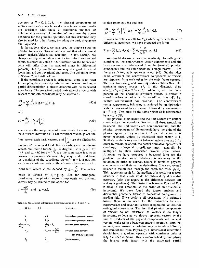
In the sections above, we have used the simplest notation possible for clarity. This notation is not that of traditional tensor analysis/differential geometry. In this section, we change our original notation in order to conform to standard forms, as shown in Table 5. Our notation for the Kronecker delta will differ from its standard usage in differential geometry, but by summation we may disregard its mixed (covariant and contravariant) character. The definition given in Section 2, will still hold here.

If the coordinate system is orthogonal, there is no need for adopting the covariant/contravariant notation, so long as partial differentiation is always balanced with its associated scale factor. The covariant partial derivative of a vector with respect to the kth coordinate may be written as

with

+ c afk =- a x k j

da'

where a' are the components of a contravariant vector, a f k is the covariant derivative of a contravariant vector, g, are the

(non-normalized) basis vectors, and are the Christoffel

symbols of the second kind. For an orthogonal coordinate system, the metric tensor, g,), is diagonal, with g, = 0 for i Zj, and g,/ = hf for i = j (h, are the same scale factors as discussed in previous sections. They may be derived from the definition of the coordinate system). If y is a position vector in a Cartesian system, the covariant basis vectors for

coordinate system x' are defined by g, =-. The metric

tensor is defined by g,) =g , ' g , . But for orthogonal coordinates, the physical vector components and the unit vectors may be related to the above by:

{jil

SY ax'

a ( i ) h,

a' =- and g, = h,&,

Table 5. Notational differences between Sections 2-4 and 5-7

86 2-4 6 5

ai a(i) (physical components of a vector)

T.. T(ij) (physical components of a tensor)

(covariant pamal derivative)

a,(a(i)) or a* (covariant derivative

a 'I a (-)or a, a,. or an

agn

'i,n ax" of a physical component)

- 'ij 'ij (Kroneckcr delta)

so that (from eqs 45a and 46):

(47)

In order to obtain results for V,a which agree with those of differential geometry, we have proposed the form:

We should discuss a point of neutrality. In orthogonal coordinates, the contravariant vector components and the basis vectors are disbalanced from the (neutral) physical components and the unit vectors by a single power (f l) of the scale factor, as is apparent in eqs (46). On the other hand, covariant and contravariant components of vectors are displaced from each other by the scale factor squared. The rule for raising and lowering indices shows this. The conjugate metric tensor, g'], is also diagonal, thus: a' = C i giJa, = C i 8.-a./h' = a j / h f , where a, are the components of the associated covariant vector. A vector in coordinate-free notation is 'balanced' or 'neutral', i.e. neither contravariant nor covariant. For contravariant vector components, balancing is achieved by multiplication with the covariant basis vectors, followed by summation: a = C i a'g,. This must be the same vector as is represented by a = Ci a(i)C,.

The physical components and the unit vectors are neither contravariant nor covariant. W e also call them neutral, or balanced. The unit vectors are non-dimensional, and the physical components (if dimensional) have the units of the physical quantity they represent. A partial derivative is never balanced, unless its associated scale factor is 1. Similarly, scale factors are not balanced unless they are 1. In order to remain balanced, the partial derivative operators of curvilinear orthogonal coordinates must generally be multiplied by their associated inverse scale factors. Although we have proposed a balanced form for the gradient operator, some disbalance is necessary in the notation, in order to express results in terms of physical components and their partial derivatives. Even so, overall balance is maintained through the combined form: Pk 3,. This makes our result for the gradient of a vector (or tensor) identical to that which would be obtained by differential geometry (with due regard t o the difference between left and right gradients). The distinction between V,a and V,a is clear in our notation, as the order of unit vectors is important. We have found the tensor analysis and differential geometry literature somewhat ambiguous re- garding this. If we perform all operations with balanced forms, there is no need for the distinction between contravariant and covariant vectors or operators, at least for orthogonal coordinates. The fact that physical components of vectors d o not transform as vectors is no longer important, so long as we always represent vectors by the sum of products of the physical components and the unit vectors, while using a balanced gradient operator. With this in mind, coordinate-free notation may be translated directly into component form. Physically, a dimensional description should have a gradient operator with consistent units of length in each direction. This is accomplished by multiplying the inverse scale factor with the associated partial

I / 6

Dow




Christoffel symbols carry terms to cancel this. This accounts for much of the simplification possible in our notation, and applies to all orthogonal coordinate systems. Another aspect of this cancellation allows particular simplification for some orthogonal coordinate systems. Unit vectors in orthogonal coordinates are tangent to the coordinate lines (curves). They possess the property:

differential operator. This is also apparent in the definition of distance in curvilinear coordiantes.

We now show how the transformation matrix, An;*, relates to the Christoffel symbols. From the notation defined above for the covariant derivative, we have:

da

Also, using our notation:

(49)

where we have used the identity, c ; k a(i)A,,&, = Cika(k)Ank,Si, which is true because i and k are dummy indices. Then for each value of i and n (1, 2, or 3) we have:

&(i) ax"

We cancel common factors of __ to yield:

a ( i ) ah; a ( k ) h; dX" + c k hk h;( in) = c a ( k ) A n k i .

T [ -$ik hi 6 -k T' ( kn] - a ( k ) A n k i ] = O.

A,ki = < ( J - 6;k hi -L. axil

(52)

Now the first term above may be included in a sum on k, if the term vanishes for k f i. So we have:

a(k ) dh. a(k)h. i (53)

This is written in a form with a(k ) as a common factor. As the vector is arbitrary, we must have the following, for each value of n, i and k:

h - 1 dh. (54)

This shows how the transformation matrix proposed in Section 2 relates to the Christoffel symbol of the second kind. For orthogonal coordinates, this Christoffel symbol reduces to

(55)

So that,

(56) This may be simplified considerably, by cancelling the first and last terms on the right-hand side, to yield:

- 1 dhi - 1 d h (57) A .=&---( j -2

k n '" h, dxk hi dx' ' nkt

The terms which cancel, going from eq. (56) to eq. (57), also occur in all gradient operations on vectors and tensors, for orthogonal coordinates. These terms arise due to the imbalance of the contravariant notation for vectors. The

a ( i ) ah. hi dx"

term: ---I, arises from hi

a - (en)] * C" = 0.

This follows from the operation a,,(C, 6*), which must vanish as 6, - 2, is constant. This places significant limits on the number of possible non-zero components of A,,;, for all orthogonal coordinate systems. Some of the non-zero Christoffel symbols do not influence the equations for the physical components in orthogonal coordinates, e.g. those arising from the form dnhn. The Christoffel symbols include some effects of the spatial dependence of the scale factors which are unimportant for descriptions using only unit vectors. Note that, for orthogonal coordinates, g,, - g, = h i . Scale factors are generally functions of space. By the product rule, we have

(59)

The covariant basis vector g, is thus not generally

orthogonal to -. We have orthogonality of these

quantities only when the scale factor h, is independent of the nth coordinate. This type of independence is only true for coordinate lines of constant curvature, as is the case for spherical and cylindrical coordinates, but not for many others (e.g. parabolic). The terms of the form d,h, cancel when converting coordinate-free equations into physical component equations in orthogonal coordinates. Some of the potentially non-zero elements of the Christoffel symbols are thus unnecessary for a description in orthogonal coordinates. In either case, our notation captures the essence needed for transforming coordinate-free equations to physical component equations with much less labour than for the notation which invokes the Christoffel symbols.

The transformation matrix, Ankit will generally have fewer non-zero entries than the Christoffel symbol, when both are evaluated for the same orthogonal coordinate system. From eq. (57), it is apparent that if all the subscripts are different, Anki will vanish. An additional property may be deduced as follows. We know that dk(&; - 8,) = 0, as the quantity in parentheses is 0 or 1. The same result must be found if we perform differentiation before contraction, thus

2% dX '/

A,;, = (bob)

This also implies that terms of the form Akii vanish. This

Dow



664 E. W . Bolton

property, and the vanishing of An, when all indices are different, implies that at most 12 of the 27 components of Anik will not vanish for orthogonal coordinates in three dimensions. Of these, only six can be independent (by eq. 60b). For the case of spherical-polar coordinates, we had six non-vanishing components with only three independent. The fact that four terms were present of the form A,, arises from the r and 8 dependence of h,, as is clear from eq. (57). It is also apparent that A,, is insensitive to the dependence of h, upon E,. This special property is not shared by the Christoffel symbols, as discussed above. From the expression above for the Christoffei symbol in orthogonal coordinates (eq. 55), we note that symbols of the form

(,f.) will vanish only if 3; hi = 0, which is the case for

spherical and cylindrical coordinates, but not for elliptic or parabolic coordinates.

6 THE FORM OF THE NAVIER-STOKES EQUATION

The Navier-Stokes equation for a Newtonian fluid with constant material properties, without invoking Stokes' hypothesis, may be written in contravariant form (Ark 1962, eq. 8.22.2) as:

I

where gmk is the conjugate metric tensor, f i is the contravariant form for the body forces per unit mass, p is the dynamic viscosity, A is the second viscosity coefficient, p is the density, u' is the Eulerian velocity (contravariant form), t is time, and p is the pressure. Perhaps the least well known of these quantities is the second viscosity coefficient, which is related to the bulk viscosity, K*, by K* = A + 2p/3. The bulk viscosity vanishes for a perfect monoatomic gas, which is effectively what is assumed under Stokes hypothesis (A = - 2p/3). The second viscosity for a number of liquids has been measured by Liebermann (1949). It may exceed the dynamic viscosity by factors ranging from 1.3 to 200, for the liquids examined by Liebermann, and is frequency dependent. We may rewrite eq. (61) in coordinate-free, vector form as (Ark 1962, eq. 8.22.4):

= pf - grad ( p ) + (A + p ) grad (div (u)) + pV*u. (62)

The distinction between V, and V, is not important in this equation. The equation Aris gives for the physical components is unnecessarily complicated (Ark 1962, eq. 8.22.5). Eq. (61), must be multiplied by g i , and summed over i to yield eq. (62). After some rather lengthy calculations, we found our notation applied to eq. (62) to be consistent with eq. (61) translated into physical components, assuming orthogonal coordinates. This consistency must be maintained by correct notations.

While developing the Navier-Stokes equation for spatially dependent viscosity, we will illustrate the

application of some useful vector identities:

V, . (V,a) = V,(V,. a) = V(V . a)

= V,(V, a) = V, - (V,a).

It is surprising that these relationships are not discussed in most fluid dynamics textbooks. Perhaps this is due to the tendency to express the equations in Cartesian coordinates, for which more general coordinate-free expressions are unnecessary. If one assumes a Newtonian fluid, the deviatoric stress tensor is linearly related to the velocity gradient tensor. The latter is decomposed into its symmetric (rate of strain tensor) and antisymmetric parts. The rate of strain tensor may be written as: E = ~ ( V U + (Vu)'), where '- denotes the transpose; or in our notation as E = $(V,u + V,u). After integrating the surface forces over a parcel, and invoking the Gauss divergence theorem, the viscous term in the equation of motion will contain terms like 2V,-(pE), or equivalently 2V,-(pE) as is symmetric. For spatially dependent viscosity we may write

2V, - (@) = 2(VLp) * E + 2pVL * (E). (64)

The calculation of (V,p) E is straightforward. We have already outlined the general form of 6, above, which may be evaluated using V,u and V,u as from eqs (7c) and (8c). Then

2(v,p) - E = 2 C en * Bn(anpc> C W k ) 2 1 * k n ik

= 2 jkn C s n j P n ( a & ) E ( j k ) @ k

Now

2p(v, ' ( E ) = p(v, v,u + v, ' VRU) (66a)

(66b) = p[VZu + V(V * u)],

where we have used the identities V,-V,u=V2u and V, . (V,u) = V(V - u), as developed below. Note that eq. (66b) does not require the distinction between V, and V,, because V,q = V,q for scalar q, and V, * u = V, - u for vector (first-order tensor) u. The identity V, (V,u) = V(V - u), is true in any coordinate system for which a metric can be defined (with well-behaved u). In rectangular coordinates this relation is trivial to derive, by changing the order of partial differentiation: C i 3,(aku,) = C i a k ( a ; U j ) . To prove this identity in curvilinear coordinates, it is most convenient to use the notation of differential geometry. Following Aris (1962, pp. 180-182), we may write twice the right divergence of the rate of strain tensor (V, - E ) in contravariant form as

which illustrates that

2v, * (E) = v, * (V,U) + v, - (V,U) = V(V - u) + v2u.

(68a)

(68b)

Dow




An analogous relation for the left divergence may also be proved. The identities, V, - (V,u) = V(V + u) = VR (VLu), may be proved for orthogonal coordinates using our notation, but the derivation is quite tedious. Two identities relating the transformation matrices are useful in this regard. They are:

- P k - Pi Anki = - Sin - Bki + S - Bik Pt kn P'k which follows from eqs (16) and (57).

As we have developed expressions for the physical components for each of the coordinate-free forms of the terms encountered in the Navier-Stokes equation, we now consider the case of spatially (and temporally) varying material properties. We write

where T is the stress tensor, which may be written as the sum of the contribution from the pressure and the deviatoric stress tensor D, as T = -pZ + D Here, Z is the idemfactor: Z = Cik (&k&zSk). For an isotropic Newtonian fluid the deviatoric stress tensor may be written as: D = AZ(V * u) + 2pE. Now we use the fact that V.(qZ) = V q , and the identities developed above to write the Navier-Stokes equation for variable material properties as:

p -+u vu =pf-Vp+pV2u+(V.u)(VA) (: - 1 + (A + p)V(V - U) + 2(Vp) - E. (72)

The form of each of these terms for arbitrary orthogonal curvilinear coordinates has already been given. For an incompressible fluid we have:

= pf - Vp + pV2u + 2(Vp) - E . (73)

7 THE SURFACE GRADIENT A N D DIVERGENCE OF A TANGENT TENSOR FIELD

Besides deriving forms for scalar representation of vector and tensor fields, Backus (1967) gives explicit forms for the surface gradient, V,, acting on tangent vector and tensor fields. We may write a second-order tangent tensor field in spherical-polar coordinates as:

(74)

where T(ab) are the physical components. We use the roman letters (a-c) to have ranges restricted to 2,3. (Our numbering of unit vectors differs from that of Backus.) The surface gradient for spherical-polar coordinates has the form:

v, = v - ?(? V) (75-3)

3

= c S C P C 2,. (c=Z)

In our notation, the right-surface gradient of a second-order tangent tensor field takes the form (in spherical-polar coordinates):

3

v.SRTS = c Pc ac(T(ab)206b)6c (76a) (a,b,c=2)

= iia&bPc 2 , [ T ( ~ b ) ] & ~ (a,b.c=Z)

+ i T(Ub)PC(Aeak&k&b&, + A,bk&,&k&,). (a,b.c=Z)

k = l (76b)

This is equivalent to eq. (2.25) of Backus (1967), if expressed in spherical-polar coordinates. The right divergence is recovered by contracting the two trailing unit vectors to yield:

3

(a .c=2)

+ T(ab)Pb(Abak&k)

v,, * Ts = c &Pc ac[T(ac)l

3

(a.b=Z) k = l

+ 5 T(ab)fic(Acbc&a). (77) (a,b,c=Z)

In spherical-polar coordinates, the ? component of this divergence yields T(22)~2A2z1 + T(33)/3,A3,, . The pressure jump of 2u/R across a spherical surface of radius R in the absence of gravity is immediately recovered (the Young- Laplace term), where u is the surface tension.

8 CONCLUSION

The simple notation presented here is a modest, but convenient, extension of notations already in common use. Differentiating vectors and tensors in curvilinear coordinates must be done with care, as the orientation of the unit vectors is spatially dependent. By the introduction of various transformation matrices (as A,, in Section 2), the calculation of expressions for the physical components from differential vector operations in spherical-polar coordinates is greatly simplified, compared to other notations. For the final translation step into usable forms, only the few non-vanishing components of the transformation matrices need be considered. The notation developed here may be applied to any orthogonal coordinate system. Although the results of most of the examples given are available in standard handbooks, the gradient and divergence of general second-order tensors given in Section 4 are not readily available elsewhere. The simplicity of the notation, as illustrated by the examples of common vector operations, provides an efficient alternative to the covariant/ contravariant notation in common use, for derivations in orthogonal curvilinear coordinates.

Dow



666 E. W. Bolton

Our quest for simple notation arose from the problem of spherical shell convection with temperature dependent viscosity, where the viscous term may contain an unusual form. We have found our notation convenient, even for performing straightforward vector operations (such as V,X), when such operations must be performed multiple times. The poloidal/toroidal decomposition of the velocity field for a Boussinesq fluid allows a reduction in the number of independent variables. This decomposition for solenoidal fields, introduced by Backus (1958), has been used in a variety of theoretical and numerical models for fluid flow in spherical shells and plane layers (e.g. Busse 1970; Clever & Busse 1974; Bolton & Busse 1985; Zhang & Busse 1989). (If mean flow is present in plane layers, the decomposition is less straightforward, but recent theoretical work addresses this problem, Schmitt & von Wahl 1992.) The reduction of the number of unknowns, however, leads to higher order equations. The Navier-Stokes equation is second order (V2u in the viscous term). The equation governing the dynamics of the toroidal field is 4th order, and that for the poloidal field is 6th order. For constant viscosity, the viscous term in the poloidal equation for spherical shell convection has the form i - 0, x V, x (V’)V, x V, x (fa). Such terms are conveniently derived in explicit form using our notation (extended as necessary to include higher order derivatives of Anik and p, than we have shown here).

We have confined our attention to orthogonal coordinate systems. With that restriction, it is possible to simplify notation for some non-Euclidean spaces as well, particularly spherical surfaces described by spherical coordinates. Our notation (using orthogonal coordinates) can be specialized for Riemannian surfaces which are embedded in Euclidean space. In addition to spherical surfaces, this includes the Riemannian surfaces of cylinders, ellipsoids, and any other surface for which an orthogonal coordinate system can be constructed. We have shown how our notation relates to that of tensor analysis/differentiaI geometry. The covariant and contravariant notation is still useful for non-orthogonal coordinates, and for proofs of some vector identities, but it can be avoided when orthogonal coordinates are adopted. Then, transformation of coordinate-free equations into equations for the physical components may be performed directly.

ACKNOWLEDGMENTS

I would like to thank Aim6 Fournier, Jeffrey Park, Ronen Plesser, Daniel Rosner and George Veronis for helpful discussions. Support was provided by the US National Science Foundation (EAR-9018215).

REFERENCES

Aki, K. & Richards, P. G., 1980. Quantitative Seismology: Theory and Methods, Vol. 1, W. H. Freeman & Co., San Francisco.

Arfken, G., 1970. Mathematical Methods for Physicists, 2nd edn, Academic Press, New York.

Aris, R., 1962. Vectors, Tensors, and the Basic Equations of Fluid Mechanics, Dover, New York.

Backus, G., 1958. A class of self-sustaining dissipative spherical dynamos, Ann. Phys., 4, 372-447.

Backus, G. E., 1967. Converting vector and tensor equations to scalar equations in spherical coordinates, Geophys. J. R. astr.

Batchelor, G . K., 1967. An Introduction to Fluid Mechanics, Cambridge University Press, Cambridge, UK.

Bolton, E. W. & Busse, F. H., 1985. Stability of convection rolls in a layer with stress-free boundaries, J. Fluid Mech., 150,

Busse, F. H., 1970. Thermal instabilities in rapidly rotating systems, J. Fluid Mech., 44, 441-460.

Clever, R. M. & Busse, F. H., 1974. Transition to time-dependent convection, J. Fluid Mech., 65, 625-645.

Edwards, D. A,, Brenner, H. & Wasan, D. T., 1991. Interfacial Transport Processes and Rheology, Butterworth-Heinemann, Boston.

Fliigge, W., 1972. Tensor Analysis and Continuum Mechanics, Springer-Verlag, New York.

Gibbs, J. W. & Wilson, E. B., 1925. Vector Analysis, Yale University Press, New Haven.

Happel, J. & Brenner, H., 1986. Low Reynolds Number Hydrodynamics, with Special Applications to Particulate Media, Martinus Nijhoff Publishers, Boston.

Liebermann, L. N., 1949. The second viscosity of liquids, Phys. Rev., 75, 1415-1422.

Mase, G. E., 1970. Schaum’s Outline of Theory and Problems in Continuum Mechanics, McGraw-Hill Book Co., New York.

Morse, P. M. & Feshbach, H., 1953. Methods of Theoretical Physics, Vol. 1, McGraw-Hill Book Co., New York.

Moon, P. H. & Spencer, D. E., 1961. Field Theory for Engineers, Van Nostrand, Princeton, NJ.

Rosner, D. E., 1986. Transport Processes in Chemically Reacting Flow Systems, Butterworths, Boston.

Schmitt, B. J. & von Wahl, W., 1992. Decomposition of solenoidal fields into poloidal fields, toroidal fields and the mean flow. Applications to the Boussenesq equations, Proc. Conf. Navier-Stokes Eq. II: Theory and Numerical Methoh, Oberwolfach: 1991, Lecture Notes in Mathematics, pp. 291-305, eds Heywood, J. G. et al., Springer-Verlag. New York.

Sokolnikoff, I. S., 1964. Tensors Analysis: Theory and Applications to Geometry and Mechanics of Continua, 2nd edn, John Wiley & Sons Inc., New York.

Synge, J . L. & Schild, A., 1949. Tensor Calculus, University of Toronto Press, Toronto.

Truesdell, C., 1953. The physical components of vectors and tensors, 2. angew. Math. Mech., 33, 345-356.

Zhang, K.-K. & Busse, F. H., 1989. Convection driven magnetohydrodynamic dynamics in rotating spherical shells, Geophys. Astrophys. Fluid Dyn., 49, 97-116.

SOC., 13, 71-101.

487-498.

Dow



a simple notation for differential vector expressions in orthogonal

Documents