a simple test for the pollution haven hypothesis · a simple test for the pollution haven...
TRANSCRIPT
University of Lausanne HEC / MSE Term Paper Academic Year 2002-2003
A Simple Test for the Pollution Haven Hypothesis Course: Applied Econometrics Author: Nicole Andréa Mathys Professor: Marius Brülhart Assistant: Aleksandar Georgiev Date: May 2003

A Simple Test for the Pollution Haven Hypothesis
1
Contents
1. INTRODUCTION .............................................................................................................2
2. THE POLLUTION HAVEN HYPOTHESIS .................................................................3
3. ECONOMETRIC ISSUES ...............................................................................................5
3.1 Missing Data.....................................................................................................................5 3.2 Unbalanced Panel (Estimation with Randomly Missing Data) ...................................7
4 DATA AND RESULTS......................................................................................................9
4.1 Data Description ..............................................................................................................9 4.2 Data Preparation ...........................................................................................................10 4.3 Regressions .....................................................................................................................13
5 CONCLUSION .................................................................................................................22
APPENDIX..............................................................................................................................26

A Simple Test for the Pollution Haven Hypothesis
2
1. Introduction
People are more and more concerned about the environment and fearful about the
environmental consequences of globalisation. The clash is frequent between policy makers
promoting their trade liberalisation programmes and globalisation opponents crying their
slogans. But what is the real impact of trade liberalisation on the environment? In this work
one of the possible effects, namely the implication predicted by the pollution haven
hypothesis (PHH) will be tested empirically. The strength of this work is that it bases its
estimates on a large number of countries over more than ten years. Also, it investigates each
“polluting industry” separately, in order to take into account the differences between them.
The aim of the present work is twofold: first, to test the PHH, and second, to deal with
missing data problems, and discussing which methods may be used in order to overcome the
latter problem.
The paper is organised as follows. In the next section, the basic idea of the pollution haven
hypothesis is presented in a Heckscher-Ohlin framework. Section three treats with
econometric concerns: the problem of missing data and, as a special case, the unbalanced
panel estimation. Section four applies the methodology to real data, in order to identify the
pollution haven effect. Finally, section five draws the conclusions and points at possible
extensions of the work.
A Simple Test for the Pollution Haven Hypothesis
3
2. The Pollution Haven Hypothesis
The pollution haven hypothesis (PHH) is a fundamental concept in the trade and the
environment literature. Several definitions have been used, but the one that will be retained
for the present empirical investigation is based on Liddle (2001). For this author the PHH is
verified if low environmental standards become a source of comparative advantage and
therefore drive shifts in trade pattern. To be more precise, what one has in mind in this
context is the following: assume developed countries are severe concerning environmental
regulation and developing countries are less strict.1 This leads to a comparative advantage in
polluting products (products that are classified to be relatively polluting, see section 4.1) for
developing countries. In this line of ideas, one could fear a “Race to the bottom”, which
predicts that countries will mutually compete environmental standards down.
An early study on the PHH is Tobey (1990), who tests in a Heckscher-Ohlin-Vanek (HOV)
framework (explained below) the impact of domestic environmental policies on trade
patterns. More precisely he regresses trade in a specific “polluting” commodity2 on country
characteristics. Tobey uses two approaches. The first one has environmental stringency as an
explanatory variable in the equation (23 countries in the sample), while the second one is a so
called omitted variable test (58 countries), where he examines the signs of the estimated error
terms. In no case, even when extending the basic HOV model of international trade with non-
homothetic preferences or scale economies and product differentiation, he finds that the
introduction of environmental control measures has caused a deviation of trade patterns from
the HOV predictions.
The HOV model is an extension of the HO model which simply predicts that a country should
export goods which use intensively the factor of production that is relatively abundant in this
country. Mani and Wheeler (1999) and Cole and Elliott (2002) show that polluting industries
are typically capital intensive. One easily accepts that developed countries are relatively
capital abundant compared to developing countries and would therefore specialise in polluting
industries. Hence, the HOV prediction of trade flows is the exact opposite of the PHH. This
1 This is consistent with the widely confirmed property that increased GDP per capita leads to a stronger concern about the environment. See for example Mani and Wheeler (1999). 2 Polluting industries are identified in function of US abatement costs.

A Simple Test for the Pollution Haven Hypothesis
4
work tries to figure out whether the coefficient on environmental stringency is significant and
has the right sign when controlling for endowment (HOV) effects.
In summary, the following estimation will be run for each polluting sector3:
itititititit EnvstringLandCapitalLabourne ������ ������ 43210
where ne: net exports
i: country i
t: year t
In contrast to Cole and Elliott (2003) the preferred specification will estimate a separate
regression for each polluting industry. Earlier work (in particular Grether and de Melo (2002)
and Mathys (2002)) suggests that an aggregate analysis hides specific patterns in each
industry. If there is indeed a PHH story in the data, it is more likely to be found at the
disaggregated level.
3 Note that in this simple specification no country-mean correction is included. This is a general equation which must be modified for the different panel estimation procedures.

A Simple Test for the Pollution Haven Hypothesis
5
3. Econometric Issues
3.1 Missing Data
Datasets are rarely complete. When working with panels it is even more likely that some
variables and/or some years are missing for the given countries4. First of all, one has to know
whether there are some reasons underlying the missing data-points. In fact, three types of
missing data can be distinguished:
� Missing Completely at Random (MCAR): There is no difference between complete
cases and incomplete cases; this would be obtained if a researcher arbitrarily discards
some raw data.
� Missing at Random (MAR): Cases with incomplete data on variable “A” differ from
cases with complete data and the missingness is related to another variable (i.e. “B”)
in the database.
� Non-ignorable: The pattern of missing data of variable “A” is not random and is not
related to other variables in the database, but to the very variable “A”.
Assume data is MCAR (or at least MAR), then one may use a method from the list below to
deal with missing data:
� Complete Case approach: Use only countries where all variables in the database are
known (disadvantage: loss of information may be important).
� Available Case analysis: use all countries where the variables of interest (for each
computation) are present (disadvantage: changing sample bases make comparisons
more difficult).
4 The enconometric issues will be presented in the context of the PHH, namely a database on countries, over years.

A Simple Test for the Pollution Haven Hypothesis
6
� Model based procedures: incorporating the missing data into the analysis (i.e. EM
(Expectation Maximisation) approach, which is an iterative two stage approach).
� Imputations Methods: the missing value is estimated by using other values of the
variables and/or cases in the sample (disadvantage: “seductive and dangerous”).
Furthermore, the imputation methods can be broken down into the following approaches:
� All-available approach: missing values are not replaced, but distribution
characteristics are imputed.
� Replacement of missing data:
o Case substitution: replace sampled country with another country not yet in
the sample.
o Mean substitution: replacing missing data points with mean value of the
variable (disadvantages: variance gets underestimated, actual distribution is
distorted, depresses the observed correlation).
o Cold Deck Imputation: Substitute a constant value from external source
(disadvantages: see mean substitution).
o Regression Imputation: using the relationships between the variables in the
dataset (disadvantages: reinforces relationships already in data which means
less general results, variance is underestimated if no error term is added,
assumes variable with missing data has strong correlation with other variables,
if no constraints computed values may fall outside the valid range for a
variable).
o Multiple Imputation: composite estimation based on several methods

A Simple Test for the Pollution Haven Hypothesis
7
This list points at the most important techniques but is far from being exhaustive. Section 4.2
will take up two methods to deal with missing data.
3.2 Unbalanced Panel (Estimation with Randomly Missing Data)
This subsection links together the missing data problem with the panel data estimation
procedures5. The fixed and the random effect estimators can both be extended to the case
where the number of years per country in the data is not identical. Then one has to compute
means over the available observations.6 “Available means” are defined in the following way:
�
�
�
�� T
tit
T
titit
i
r
yry
1
1 and
�
�
�
�� T
tit
T
titit
i
r
xrx
1
1
where rit is the indicator variable taking 1 if (xit, yit) is observed and 0 otherwise. The fixed effect estimator becomes:
� �� ���� ��
�
�
�����T
t
T
tiitiitit
N
iiitiitit
N
iFE yyxxrxxxxr
1 11
1’
1
))(())((�̂
Hence, one must just make sure that the sums are taken over the available observations only.
The random effect estimator can be obtained form the following equation (note that the
definition of the Greek letters is slightly different compared to the random effects presentation
in appendix A):
5 For a summary on panel data estimations read appendix A. 6 Note that each country should at least report data for two years.
A Simple Test for the Pollution Haven Hypothesis
8
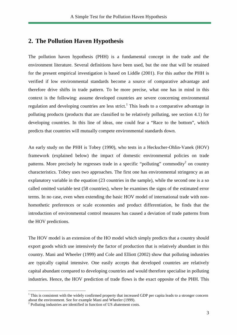
� ������ ���
�
��
����T
t
N
ii
T
tit
N
i
N
iiit
N
iGLS
1 111
1
11
)()(ˆ �����
where )’)(( iitiititit xxxxr ����
)’)(( xxxxT iiiii ��� ��
))(( iitiititit yyxxr ����
))(( yyxxT iiiii ��� ��
22
2
��
�
���
�i
i T��
��
�T
titi rT
1
(number of periods country i is observed)
Thus, in fact one simply has to replace T by Ti and therefore take sums and means over the
available data.
Fortunately stata7 uses the extended estimators and is consequently insensible to unbalanced
panels. Hence in the practical part these issues need not be taken up again.
A Simple Test for the Pollution Haven Hypothesis
9
4 Data and Results
4.1 Data Description
Data covers 13 years (1983-1995) for over 50 developed and developing countries.7 Basically
there are three different categories of data. Firstly, the explained variable is net exports
(exports-imports)8 of the five most polluting industries. The classification of polluting
industries has been elaborated by Mani and Wheeler (1999) and they take into account
emission intensities per unit of output in three different domains (conventional air pollutants,
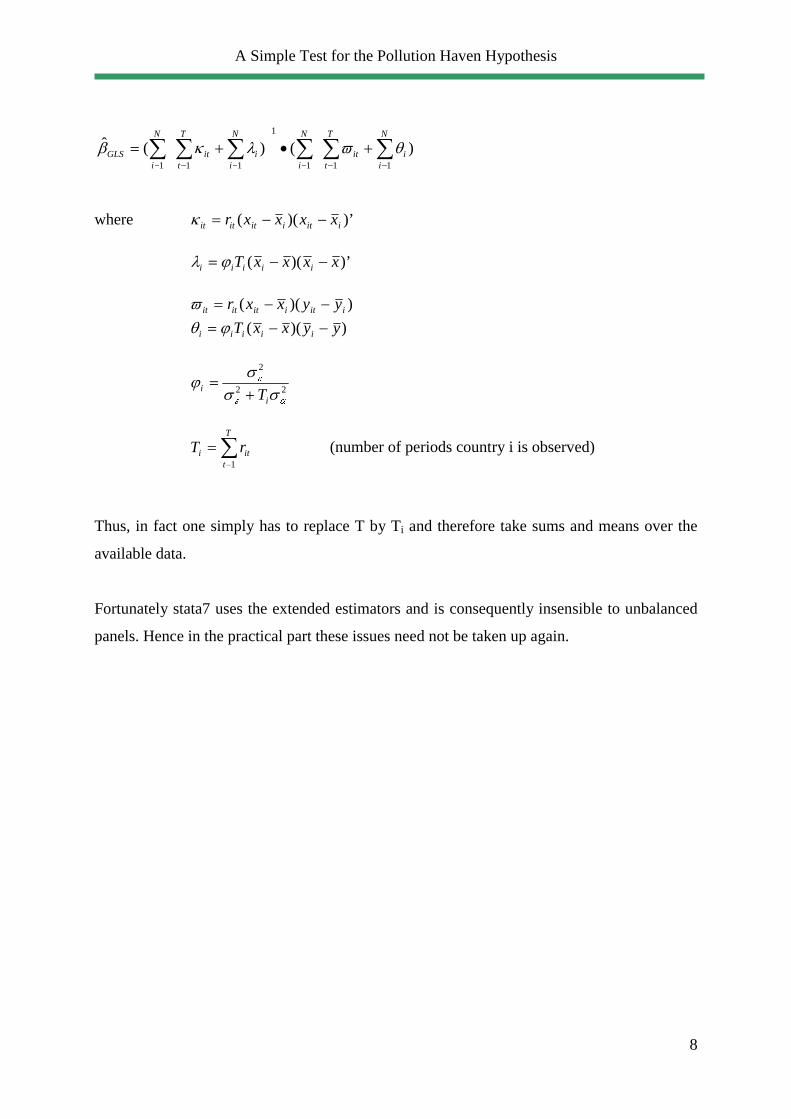
water pollutants and heavy metals). Based on the 3-digit-ISIC classification they found the
following five most heavily polluting industries:
Table 1: Categories of polluting products
Then there are two groups of explanatory variables. One group contains variables relative to
the classical Heckscher-Ohlin-Vanek (HOV) trade model, while the other group captures the
pollution haven hypothesis. The variables that account for HOV theory are relative factor
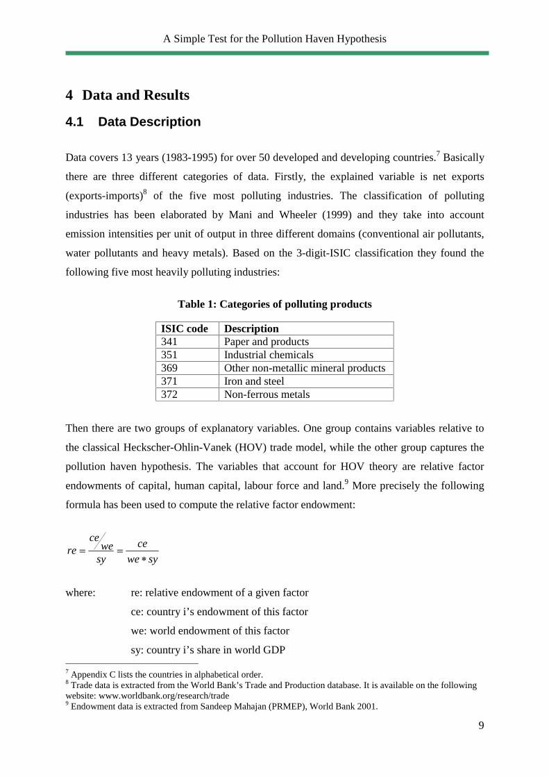
endowments of capital, human capital, labour force and land.9 More precisely the following
formula has been used to compute the relative factor endowment:
sywe
ce
sywe
cere
���
where: re: relative endowment of a given factor
ce: country i’s endowment of this factor
we: world endowment of this factor
sy: country i’s share in world GDP 7 Appendix C lists the countries in alphabetical order. 8 Trade data is extracted from the World Bank’s Trade and Production database. It is available on the following website: www.worldbank.org/research/trade 9 Endowment data is extracted from Sandeep Mahajan (PRMEP), World Bank 2001.
ISIC code Description 341 Paper and products 351 Industrial chemicals 369 Other non-metallic mineral products 371 Iron and steel 372 Non-ferrous metals
A Simple Test for the Pollution Haven Hypothesis
10
In words, the relative endowment in each factor has been defined as the ratio between the
country’s share of endowment of the factor and the share of the country in world GDP.
Equivalently, it is the ratio between actual endowment and theoretical endowment. This is
very similar to the relative endowments defined by Vanek but it has the advantage that it is
comparable over factors.
Finally, the variable of interest in this work is clearly the one capturing environmental
stringency. Unfortunately it is difficult to get a good measure of environmental stringency and
even more so, if one wants the data to have a panel structure. Here the average maximum lead
content of gasoline has been used. The database has been elaborated by Grether and Mathys
(2002) on the basis of Octel’s Worldwide Gasoline Survey. More precisely the average has
been worked out by using different types of gasoline and weighting them by their market
share. Therefore, the proxy constructed takes into account the importance of the different
types of gasoline in the overall market. If one admits that it is generally more costly to
produce gasoline with low lead contents, the selected variables represents not only the
maximum lead content observed, but also, and this is the important feature, in some sense the
enforced legal limit of lead content in gasoline. Since it is impossible for the moment to get a
good global index of environmental stringency, the average maximum lead content represents
at least one of the most important environmental policies. Note also that Damania et al (2000)
qualified the lead content in gasoline as the “most viable dynamic consumption proxy” for
environmental stringency at the country level.
4.2 Data Preparation
The preparation of the three different variable-types will be discussed in turn. The database
containing the maximum average lead content has been purified completely. As the data has
been entered by students, some checks based on simple error structures have been done. Then,
the market share was missing in some cases. Appendix E indicates the two step procedure
used to impute the 78 missing data points (out of 4332).
A Simple Test for the Pollution Haven Hypothesis
11
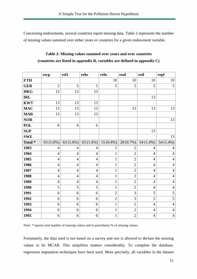
Concerning endowments, several countries report missing data. Table 2 represents the number
of missing values summed over either years or countries for a given endowment variable.
Table 2: Missing values summed over years and over countries
(countries are listed in appendix B, variables are defined in appendix C)
recp rel1 rehc reln real reil repl ETH 10 10 10 10
GER 5 5 5 5 5 5 5
HKG 13 13 13
IRL 13
KWT 13 13 13
MAC 13 13 13 13 13 13
MAR 13 13 13
NOR 13
POL 6 6 6
SGP 13
SWE 13
Total * 63 (1.6%) 63 (1.6%) 63 (1.6%) 15 (0.4%) 28 (0.7%) 54 (1.4%) 54 (1.4%)
1983 4 4 4 1 2 4 4
1984 4 4 4 1 2 4 4
1985 4 4 4 1 2 4 4
1986 4 4 4 1 2 4 4
1987 4 4 4 1 2 4 4
1988 4 4 4 1 2 4 4
1989 4 4 4 1 2 4 4
1990 5 5 5 1 2 4 4
1991 6 6 6 2 3 5 5
1992 6 6 6 2 3 5 5
1993 6 6 6 1 2 4 4
1994 6 6 6 1 2 4 4
1995 6 6 6 1 2 4 4
Note: * reports total number of missing values and in parenthesis % of missing values.
Fortunately, the data used is not based on a survey and one is allowed to declare the missing
values to be MCAR. This simplifies matters considerably. To complete the database,
regression imputation techniques have been used. More precisely, all variables in the dataset
A Simple Test for the Pollution Haven Hypothesis
12
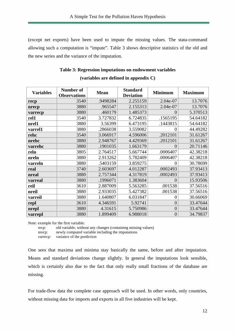
(except net exports) have been used to impute the missing values. The stata-command
allowing such a computation is “impute”. Table 3 shows descriptive statistics of the old and
the new series and the variance of the imputation.
Table 3: Regression imputations on endowment variables
(variables are defined in appendix C)
Variables Number of Observations
Mean Standard Deviation
Minimum Maximum
recp 3540 .9498284 2.255159 2.04e-07 13.7076 nrecp 3880 .965547 2.155313 2.04e-07 13.7076 varrecp 3880 .460179 1.485373 0 5.370513 rel1 3540 3.727832 6.724835 .1565195 54.64182 nrel1 3880 3.56399 6.473195 .1443815 54.64182 varrel1 3880 .2866038 3.559082 0 44.49282 rehc 3540 3.066917 4.596006 .2012101 31.61267 nrehc 3880 2.948767 4.429369 .2012101 31.61267 varrehc 3880 .1901035 1.663179 0 20.71146 reln 3805 2.764517 5.667744 .0006407 42.38218 nreln 3880 2.913262 5.782409 .0006407 42.38218 varreln 3880 .5403159 3.859275 0 30.78699 real 3740 2.603697 4.012287 .0002493 37.93413 nreal 3880 2.757344 4.317819 .0002493 37.93413 varreal 3880 .1996071 1.383604 0 15.93506 reil 3610 2.887009 5.563285 .001538 37.56516 nreil 3880 2.933035 5.427382 .001538 37.56516 varreil 3880 1.640807 6.031847 0 30.66069 repl 3610 4.346591 5.92741 0 33.47644 nrepl 3880 4.31615 5.750986 0 33.47644 varrepl 3880 1.899409 6.988018 0 34.79837 Note: example for the first variable: recp: old variable, without any changes (containing missing values) nrecp: newly computed variable including the imputations varrecp: variance of the prediction
One sees that maxima and minima stay basically the same, before and after imputation.
Means and standard deviations change slightly. In general the imputations look sensible,
which is certainly also due to the fact that only really small fractions of the database are
missing.
For trade-flow data the complete case approach will be used. In other words, only countries,
without missing data for imports and exports in all five industries will be kept.
A Simple Test for the Pollution Haven Hypothesis
13
4.3 Regressions
First of all one wants to know whether the data has indeed a panel structure. For that reason it
is interesting to look at the summary statistics which decompose the overall variation into the
between and the within variation (these results can be found in appendix F). The listed
variables report variation between countries as well as variation for each country over the
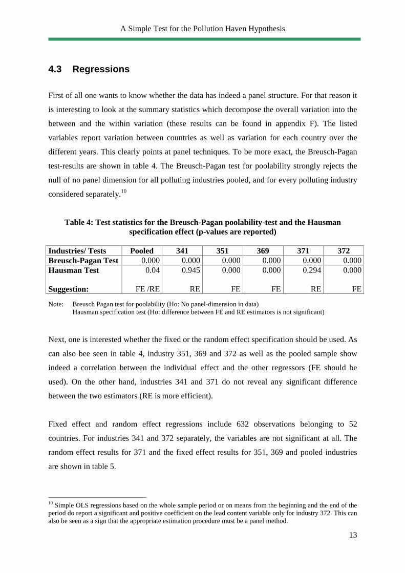
different years. This clearly points at panel techniques. To be more exact, the Breusch-Pagan
test-results are shown in table 4. The Breusch-Pagan test for poolability strongly rejects the
null of no panel dimension for all polluting industries pooled, and for every polluting industry
considered separately.10
Table 4: Test statistics for the Breusch-Pagan poolability-test and the Hausman specification effect (p-values are reported)
Industries/ Tests Pooled 341 351 369 371 372 Breusch-Pagan Test 0.000 0.000 0.000 0.000 0.000 0.000 Hausman Test Suggestion:
0.04
FE /RE
0.945
RE
0.000
FE
0.000
FE
0.294
RE
0.000
FE Note: Breusch Pagan test for poolability (Ho: No panel-dimension in data) Hausman specification test (Ho: difference between FE and RE estimators is not significant) Next, one is interested whether the fixed or the random effect specification should be used. As
can also bee seen in table 4, industry 351, 369 and 372 as well as the pooled sample show
indeed a correlation between the individual effect and the other regressors (FE should be
used). On the other hand, industries 341 and 371 do not reveal any significant difference
between the two estimators (RE is more efficient).
Fixed effect and random effect regressions include 632 observations belonging to 52
countries. For industries 341 and 372 separately, the variables are not significant at all. The
random effect results for 371 and the fixed effect results for 351, 369 and pooled industries
are shown in table 5.
10 Simple OLS regressions based on the whole sample period or on means from the beginning and the end of the period do report a significant and positive coefficient on the lead content variable only for industry 372. This can also be seen as a sign that the appropriate estimation procedure must be a panel method.

A Simple Test for the Pollution Haven Hypothesis
14
Table 5: Regresion results from FE and RE estimations (variables are defined in appendix C)
Explanatory Variable
Pooled-FE1 351-FE 369-FE 371-RE
lead 1578017** 1092036** -86083 432604** recp NS NS -91426** NS rel1 NS NS NS -160509 rehc NS -456608* 84132 NS real 373921* 166300* NS 104478* reil NS NS NS NS repl NS NS NS NS R2 within R2 overall
.05 .001
.08 .001
.06 .2
.04
.01 Note: the sample includes 632 observations from 52 countries. NS: not significant. No symbol: significant at the 10% level. * significant at the 5% level. ** significant at the 1% level. 1 RE estimates are similar and thus not presented. The coefficient on the maximum lead content is significant. However, the sign is not always
the same, more precisely, results suggest that 351 and 371 increase net exports as
environmental stringency goes down (in favour of PHH) and the opposite is true for 369
(against PHH). Additionally in industry 351, increased relative endowment of skilled labour
decreases net exports and increased relative endowment of arable land increase net exports. In
industry 369 increased capital endowment leads to fewer net exports. Finally industry 371
decreases net exports with higher unskilled labour endowment and increases the dependent
variable with higher arable land endowment. However, the interpretation of the endowment
coefficients is not straightforward. The HOV variables are included in order to control for
endowment effects but the coefficient of interest is clearly the one on environmental policy.
In sum, these regression results are not really convincing (look also at the R2). The problem
could be due to the violation of the homoskedasticity assumption, which sounds sensible
when thinking about the large differences between the countries in the sample.
Heteroskedasticity implies that the estimators are no longer “best” nor “minimum variance”.
In fact when looking at the residual-graph of a FE regression (see graphic 1), it appears
clearly, that assuming homoskedastic error terms is wrong.

A Simple Test for the Pollution Haven Hypothesis
15
Graphic 1: Residual graph for industry 372 for 9 selected countries
Res
idua
ls
id1 115
-1.3e+06
2.2e+06
Therefore, GLS estimations allowing for heteroskedasticity have been computed. Results are
reported in table 6. However, as the data set contains few years compared to the number of
countries, FGL estimations are likely to lead to “overconfidence”. Nevertheless, some time
will be spent on these results.11
11 Note that similar works using roughly the same number of countries and time periods also use the FGLS estimation method. See for example Damania et al (2000).

A Simple Test for the Pollution Haven Hypothesis
16
Table 6: Regression results
(variables are defined in appendix C)
372b
2248
9**
2864
3**
NS
NS
-278
26**
-2
5316
**
2643
7*
2425
4*
2103
0**
1816
2**
NS
NS
NS
NS
-816
9 -9
777
632
/ 52
757
/ 62
372a
2768
0**
2915
7**
NS
NS
NS-
1039
*
NS
NS
9473
**
5434
**
-886
9 -9
774
684
/ 56
757
/ 62
371b
1214
76**
12
8496
**
NS
NS
-690
57**
-5
9652
**
8164
7*
6949
4**
3345
6**
3085
9**
3285
0**
2163
9**
-106
33*
NS
-858
7 -1
0278
632
/ 52
757
/ 62
371a
1773
30**
16
2734
**
NS
NS
-478
77*
-400
27**
6845
3*
5990
1**
NS
NS
-929
8 -1
0270
684
/ 56
757
/ 62
369
NS
NS
-211
31**
-2
2555
**
-347
20**
-1
9643
**
5141
6**
3145
5**
NS
NS
-841
4 -9
267
684
/ 56
757
/ 62
351
4550
70**
45
5711
**
NS
NS
8101
4**
NS
-213
937*
* -6
6727
1140
76**
53
265*
*
-969
4 -1
0723
684
/ 56
757
/ 62
341b
7577
6**
7542
0**
2379
0*
2148
1*
1922
6**
9888
*
-413
20**
-2
6375
**
1409
3**
8650
**
-899
5 -9
917
684
/ 56
757
/ 62
341a
7493
3**
7611
9**
2086
3*
2284
2*
2603
6**
1725
1**
-468
35**
-3
6313
**
1359
5 61
68**
-899
7 -9
914
684
/ 56
757
/ 62
Poo
led
5914
13**
58
3297
**
NS
NS
NS
1342
30**
NS
1071
90
1622
97**
10
5175
**
-101
56
-112
32
684
/ 56
757
/ 62
lead
recp
rel1
rehc
reln
real
reil
repl
Log
Lik
elih
ood
Obs
erva
tion
s/C
ount
ries
Not
e: A
ll m
odel
s us
e FG
LS
with
mea
n-co
rrec
tion
for
each
cou
ntry
. C
oeff
icie
nt in
fir
st r
ow: u
nbal
ance
d pa
nel d
ata,
sec
ond
row
coe
ffic
ient
s: i
mpu
ted
data
.
N
S:
not
sig
nifi
cant
.
N
o sy
mbo
l: si
gnif
ican
t at t
he 1
0% le
vel.
*
sig
nifi
cant
at t
he 5
% le
vel.
**
sig
nifi
cant
at t
he 1
% le
vel.

A Simple Test for the Pollution Haven Hypothesis
17
All coefficients on the lead variable (except for industry 369) are positive and significant at
the 1% level. This clearly supports the PHH; a higher maximum lead content and therefore
more lenient regulation leads to higher net exports in these polluting industries.
Capital endowment is only significant for industries 341 and 369. The higher the endowment,
the higher net exports for 341 and the contrary for 369. This poor result is quite surprising as
it was argued that polluting industries are capital intensive and should therefore strongly
depend on that endowment.
Unskilled labour endowment has a positive coefficient for the pooled regression and the
industries 341 and 369. The remaining industries report a negative effect of this endowment.
How could one interpret a negative coefficient on endowments? A possible explanation would
be that an increase in total unskilled labour force has a positive effect on the remuneration of
the factor which is intensively used in this industry and by this bias leads to a decrease of the
comparative advantage and therefore a lower level of net exports.
Skilled labour is non-significant for the pooled regression and has a negative coefficient for
industries 341 and 351. The other industries report positive coefficients.
Total land is most of the time not significant. When splitting the different types of land , the
significant and also positive coefficient is attributed to arable land.
The second row in the result table (table 6) reports the coefficients when imputed data (see
section 4.2) have been used. Results differ only slightly. For the pooled industries skilled and
unskilled labour endowment become significant. On the other hand, for industry 351 unskilled
labour and for industry 371 the coefficient on permanent cropland becomes non significant. In
general, the magnitude of the coefficients is unchanged for the environmental stringency
proxy, but the coefficients are smaller for the endowment variables.
A Simple Test for the Pollution Haven Hypothesis
18
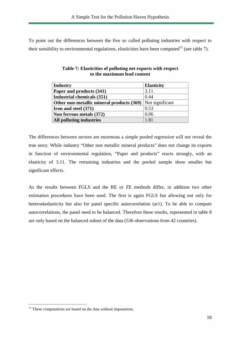
To point out the differences between the five so called polluting industries with respect to
their sensibility to environmental regulations, elasticities have been computed12 (see table 7).
Table 7: Elasticities of polluting net exports with respect to the maximum lead content
Industry Elasticity Paper and products (341) 3.11 Industrial chemicals (351) 0.44 Other non-metallic mineral products (369) Not significant Iron and steel (371) 0.53 Non ferrous metals (372) 0.06 All polluting industries 1.81
The differences between sectors are enormous a simple pooled regression will not reveal the
true story. While industry “Other non metallic mineral products” does not change its exports
in function of environmental regulation, “Paper and products” reacts strongly, with an
elasticity of 3.11. The remaining industries and the pooled sample show smaller but
significant effects.
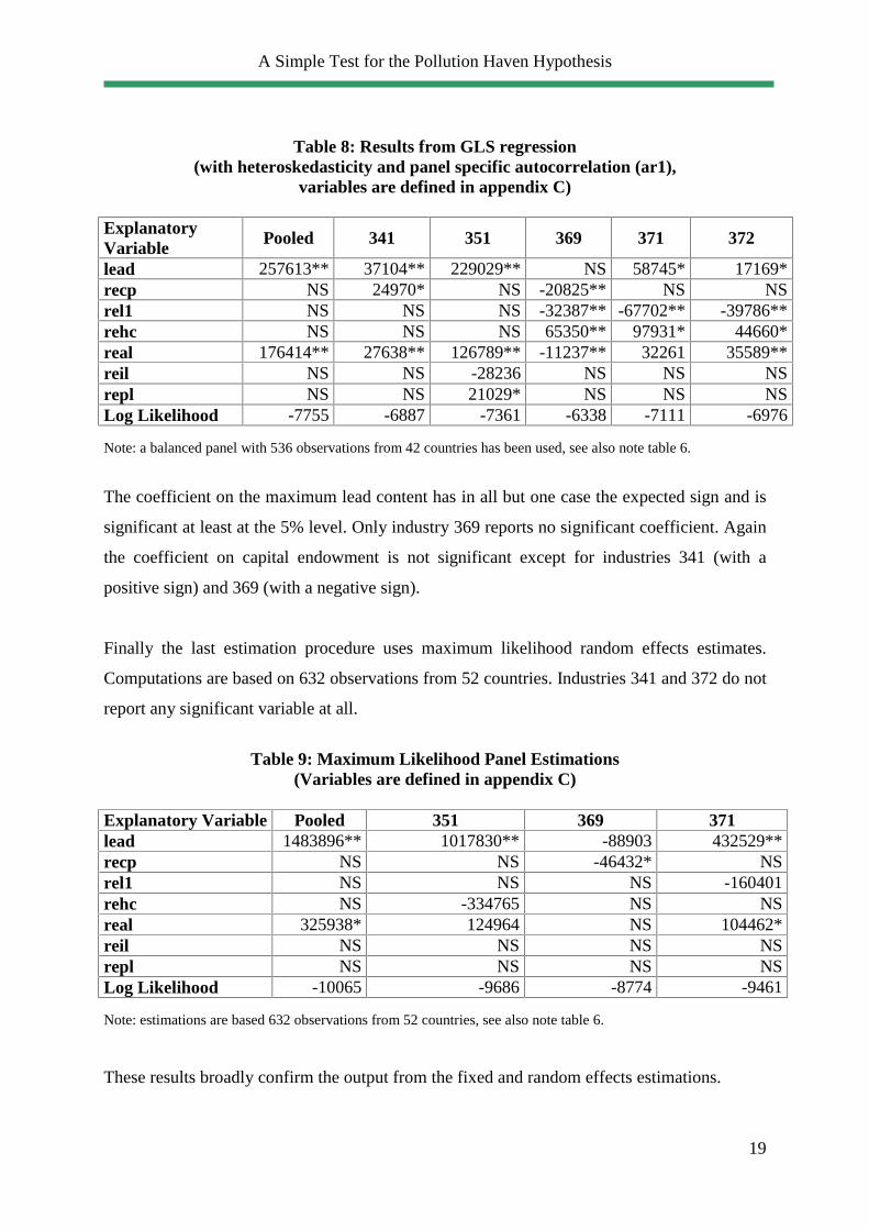
As the results between FGLS and the RE or FE methods differ, in addition two other
estimation procedures have been used. The first is again FGLS but allowing not only for
heteroskedasticity but also for panel specific autocorrelation (ar1). To be able to compute
autocorrelations, the panel need to be balanced. Therefore these results, represented in table 8
are only based on the balanced subset of the data (536 observations from 42 countries).
12 These computations are based on the data without imputations.
A Simple Test for the Pollution Haven Hypothesis
19
Table 8: Results from GLS regression (with heteroskedasticity and panel specific autocorrelation (ar1),
variables are defined in appendix C) Explanatory Variable
Pooled 341 351 369 371 372
lead 257613** 37104** 229029** NS 58745* 17169* recp NS 24970* NS -20825** NS NS rel1 NS NS NS -32387** -67702** -39786** rehc NS NS NS 65350** 97931* 44660* real 176414** 27638** 126789** -11237** 32261 35589** reil NS NS -28236 NS NS NS repl NS NS 21029* NS NS NS Log Likelihood -7755 -6887 -7361 -6338 -7111 -6976 Note: a balanced panel with 536 observations from 42 countries has been used, see also note table 6.
The coefficient on the maximum lead content has in all but one case the expected sign and is
significant at least at the 5% level. Only industry 369 reports no significant coefficient. Again
the coefficient on capital endowment is not significant except for industries 341 (with a
positive sign) and 369 (with a negative sign).
Finally the last estimation procedure uses maximum likelihood random effects estimates.
Computations are based on 632 observations from 52 countries. Industries 341 and 372 do not
report any significant variable at all.
Table 9: Maximum Likelihood Panel Estimations
(Variables are defined in appendix C) Explanatory Variable Pooled 351 369 371 lead 1483896** 1017830** -88903 432529** recp NS NS -46432* NS rel1 NS NS NS -160401 rehc NS -334765 NS NS real 325938* 124964 NS 104462* reil NS NS NS NS repl NS NS NS NS Log Likelihood -10065 -9686 -8774 -9461 Note: estimations are based 632 observations from 52 countries, see also note table 6.
These results broadly confirm the output from the fixed and random effects estimations.

A Simple Test for the Pollution Haven Hypothesis
20
Table 10 summarises all the results obtained. The pooled regression shows in any method a
positive and significant coefficient on the environmental policy variable. Also, the higher
relative endowments of arable land, the higher net exports. Industry 341 shows only in the
FGL regressions a PHH effect. It has a positive coefficient on relative capital and arable land.
Then industry 351 shows PHH effect throughout and has a positive coefficient on relative
arable land and a negative coefficient on relative human capital.
Table 10: Synthesis of Regression Results
(variables are defined in appendix C)
ML
E-R
E
+ v
e
real
- - - - + v
e
real
rehc
- ve
- recp
+ v
e
real
rel1
- - -
FG
L
(wit
h ar
1)
+ v
e
real
- + v
e
recp
, rea
l
- + v
e
real
, rep
l
reil
- rehc
recp
, rel
1, r
eal
+ v
e
rehc
, rea
l
rel1
+ v
e
rehc
, rea
l
rel1
FG
LS
+ v
e
real
- + v
e
reca
p, r
el1,
rea
l
rehc
+ v
e
rel1
, rea
l
rehc
- rehc
recp
, rel
1
+ v
e
rehc
, rea
l, re
il
rel1
, rep
l
+ v
e
rehc
, rea
l
rel1
FE
/ R
E
+ v
e
real
- - - - + v
e
real
rehc
- ve
rehc
recp
+ v
e
real
rel1
- - -
Lea
d 1
+ H
OV
2
- H
OV
3
Lea
d
+ H
OV
- H
OV
Lea
d
+ H
OV
- H
OV
Lea
d
+ H
OV
- H
OV
Lea
d
+ H
OV
- H
OV
Lea
d
+ H
OV
- H
OV
Indu
stry
Poo
led
341
351
369
371
372
Not
e: 1 R
epor
ts th
e si
gn o
f th
e si
gnif
ican
t coe
ffic
ient
on
the
lead
con
tent
var
iabl
e.
2
Rep
orts
the
vari
able
s th
at h
ave
a si
gnif
ican
t pos
itive
coe
ffic
ient
.
3 Rep
orts
the
vari
able
s th
at h
ave
a si
gnif
ican
t neg
ativ
e co
effi
cien
t.

A Simple Test for the Pollution Haven Hypothesis
21
Industry 369 shows rather the contrary of the PHH and it reacts in the opposite direction to
endowment changes compared to industry 351. Industry 371 reports again strong evidence for
the PHH. In addition, it has a positive coefficient on arable land and a negative coefficient on
the labour force. Finally, industry 372 shows evidence for the PHH in two out of four
regressions and has a positive coefficient on arable land and human capital and a negative
coefficient on the unskilled labour force.
To sum up, there is strong evidence for the PHH for all industries qualified as polluting
except “Other non-metallic mineral products”.

A Simple Test for the Pollution Haven Hypothesis
22
5 Conclusion
Evidence based on a panel of 52 countries over more than 10 years suggests that in four out of
five polluting industries there exists indeed a pollution haven hypothesis effect. This means
that lower environmental standards increase (through revealed comparative advantages) net
exports in polluting sectors.
However, the method used to test the PHH is fairly simple. The only thing it does, is
controlling for endowment driven trade (HOV). The test could be improved in several
directions. First of all it has been shown by Ederington and Minier (2003) that environmental
stringency is in fact itself endogeneous and therefore a simultaneous equation estimation
(with and additional equation explaining environmental policy by political economy
variables) would be more appropriate.
Secondly, regressions would certainly be improved when controlling for Ricardian
differences. More precisely, HOV assumes that all countries have the same technologies;
which is clearly not true in reality. The method used by Trefler (1995) could give better
results.
Thirdly, in order to get a clear-cut contrast between “dirty” and “clean” sectors, it would be
helpful to apply all the estimations also to the five cleanest sectors.
Fourthly and finally, on the data side, some improvements would be welcome. Relying on
alternative data sources would increase the confidence one can have in the conclusions drawn
on this problematic.
A Simple Test for the Pollution Haven Hypothesis
23
References
Antweiler, W., B. R. Copeland and M. S. Taylor (2001), “Is Free Trade Good for the
Environment?”, The American Economic Review, Vol. 91(4), pp. 877-908.
Arellano, M. (2000), “Panel Data Econometrics”, Draft handed out at a Summer-Course at the
Studienzentrum Gerzensee 2002.
Birdsall, N. and Wheeler (1993), “Trade Policy and Industrial Pollution in Latin America:
Where are the Pollution Havens?”, Journal of Environment and Development, Vol.2, 1, pp.
137-150.
Brülhart, M. (2003), “Panel Data Models”; lecture handout for Applied Econometrics.
Cole, M.A: (2000), “Air Pollution and « Dirty » Industries : How and Why does The
Composition of Manufacturing Output Change with Economic Development?”
Environmental Resource Economics, Vol. 17, pp.109-123.
Cole, M.A. and R.J.R Elliott (2000), “Do Environmental Regulations Influence Trade
Patterns? Testing Old and New Trade Theories”, mimeo, University of Birmingham.
Cole, M.A. and R.J.R Elliott (2002), “FDI and the Capital Intensity of “Dirty” Sectors: A
Missing Piece of the Pollution Haven Puzzle”, mimeo, University of Birmingham.
Cole, M.A. and R.J.R Elliott (2003), “Determining the Trade-Environment Composition
Effect: The Role of Capital, Labour and Environmental Regulations”, Journal of
Environmental Economics and Management, forthcoming.
Copeland, B.R. (2000), “Trade and environment: policy linkages”, Environment and
Development Economics, Vol. 5, pp. 405-432.

A Simple Test for the Pollution Haven Hypothesis
24
Copeland, B.R. and M. S. Taylor (1994), “North-South Trade and the Environment”, The
Quarterly Journal of Economics, Vol. 109, pp. 755-787.
Copeland, B.R. and M. S. Taylor (2001), “International Trade and the Environment: A
Framework for Analysis”, NBER N°8540.
Damania, R., P.G. Fredriksson and J.A. List (2000), Trade Liberalization, Corruption and
Environmental Policy Formation: theory and Evidence, Centre for International Economic
Studies, Discussion Paper No. 0047, Adelaide University, Australia.
Dijkstra, B.R. (1999), The Political Economy of Environmental Policy, Edward Elgar,
Cheltenham, UK.
Ederington, J. and J. Minier (2003), Is Environmental Policy a Secondary Trade Barrier? An
Empirical Analysis, Canadian Journal of Economics (forthcoming).
Greene, W. H. (2000), Econometric Analysis, Prentice-Hall, New Jersey.
Grether, J.-M. and J. de Melo (2002), “Globalization and dirty industries: do pollution havens
matter?”, Paper presented at the CEPR/NBER International Seminar on International Trade
“Challenges to Globalization” in Stockholm.
Grether, J.-M. and N. Mathys (2002), Lead content of gasoline 1983-1995, original data taken
from “Worldwide Gasoline Survey” published annually by OCTEL (GB).
Liddle, B. (2001), “ Free trade and the environment-development system”, Ecological
Economics, Vol. 39, pp.21-36.
Low, P. (1992), International Trade and the Environment, World Bank, Washington D.C.
Low, P. and A. Yeats (1992), “Do “Dirty” Industries Migrate?”, In Low, P. (Ed), International
Trade and the Environment, World Bank.

A Simple Test for the Pollution Haven Hypothesis
25
Mani, M. and D. Wheeler (1999), “In Search of Pollution Havens? Dirty Industry in the
World Economy, 1960-1995, in P. G. Fredriksson (ed), Trade, Global Policy, and the
Environment, Discussion Paper, N°402, Washington D.C.: World Bank.
Mathys, N. (2002), “In Search of Evidence for the Pollution Haven Hypothesis”, Mémoire de
Licence, Université de Neuchâtel.
Nicita, A. and M. Olarreaga (2001), “Trade and Production, 1976-1999”, Paper that
accompanies Trade and Production Database (httpp://www.worldbank.org/research/trade).
Nordström, H. and S. Vaughan (1999), “Trade and Environment”, Special Studies 4, World
Trade Organisation, Geneva.
Olson, M., (1965), The Logic of Collective Action, Harvard University Press, Cambridge.
Tobey, J. (1990), “The Effects of Domestic Environmental Policies on Patterns of World
Trade : En Empirical Test”, Kyklos, Vol. 43 (2), pp. 191-209.
Trefler, D. (1993), “Trade Liberalization and the Theory of Endogenous Protection: An
Econometric Study of U.S. Import Policy”, Journal of Political Economy, Vol. 101 (1), pp.
138-160.
Trefler, D. (1995), “The Case of Missing Trade and Other Mysteries ”, American Economic
Review, Vol. 85, pp. 1029-1046.
Van Beers, C. and C. van den Berg (1997), “An empirical multi-country analysis of the
impact of environmental regulations on foreign trade”, Kyklos, Vol. 50, pp..
Verbeek, M. (2000), A Guide to Modern Econometrics, John Wiley, Chichester.

A Simple Test for the Pollution Haven Hypothesis
26
Appendix
Appendix A : Panel Econometrics
Introduction
Whenever data has both time-series and cross-sectional variation, it is qualified as panel data.
In this case it is possible to look at changes on a “country”13 level. Arellano (2000) points at
two different motivations for panel data estimations. Firstly, panel data allows to control for
unobserved time-invariant heterogeneity in cross-sectional models. Secondly, panels enable
econometricians to study the dynamics of cross-sectional data sets. These two motivations can
directly be related to the two strands in the literature, fixed effects and random effects. The
two models are explained next.
Fixed Effects Model
This is a�������������������� �� ������������������������������� ���������� i). The model
can be written as follows:
ititiit xy �� ��� ’ ),0(~ 2�
�� IIDit
where i=1, ..., N (country i)
t=1, …,T (time period t)
This model is also obtained by using an OLS regression with a dummy variable for each
country. Hence, the estimator for the slope coefficients are known as the least squares dummy
variable (LSDV) estimator. One gets also the same results when using a regression in
deviations from country-means. This model eliminates thus country effects and can be written
in the following way: 13 Cross-sectional units can be thought of as individuals, households, firms, industries or countries to list just some of the possibilities. According to the empirical part of this work, countries will be referred to.

A Simple Test for the Pollution Haven Hypothesis
27
)()( ’iitiitiit xxyy ��� �����
where bars indicate non weighted means of the variables.
The latter transformation is the so called within or fixed effect transformation. The
corresponding estimator is the following:
� �� ���� ��
�
�
�����T
t
T
tiitiit
N
iiitiit
N
iFE yyxxxxxx
1 11
1’
1
))(())((�̂
If all the xit��������������������� it, the estimator is unbiased.
Basically, a model with fixed effects gives attention to differences “within” countries.
However the initial specification on � implies that a change in the explanatory variables
should have the same effect whether this variation changes from one period to the other or
from one country to the other. From that the interest of an alternative approach, the random
effects model, which relies also on cross-country variation.
Random Effects Model
One possible interpretation of the error term in a regression is that it represents all variables
that do presumably affect the dependent variable but are not explicitly introduced as
����������� ����������� ��� ����� ������� ���� ������ ��� ��� � ����� � i) is a random factor
independently and identically distributed over countries. Hence, the so called random effects
model can be written as:
itiitit xy �� ���� ’ ),0(~ 2�
�� IIDit ; ),0(~ 2�
� IIDi
The error term ( iti � � ) is made up of two components: a country specific component that
does not vary over time and a country and time specific component that is assumed to be

A Simple Test for the Pollution Haven Hypothesis
28
uncorrelated over time. Moreover, the two components are assumed to be mutually
independent and independent of xjs (for all j and s). If the assumptions are confirmed, the
intercept and slope estimates are unbiased and consistent. However, the structure of the error
term implies autocorrelation which leads to incorrect OLS standard errors (except if 02 ��
� ).
The GLS estimator is more efficient because it uses the particular structure of the error
covariance matrix (see the lecture handout for the Variance-Covariance matrix).
The random effect estimator is in fact a weighted average of the fixed effect (within)
estimator and the between estimator (defined below) where the weight depends on the relative
variances of the two estimators. Therefore one can write:
FEkBRE I ��� ˆ)(ˆ ���
������ ��������������������������������������������������������������� ������ �����������
B�̂ .
The between estimator is defined as follows:
� �� �� �
� �����N
i
N
iiiiiB yyxxxxxx
1 1
1’ ))(())((�̂
The between estimator ignores any information within countries. In fact it is the OLS
estimator in a model for individual means:
iiii xy �� ���� ’ for i= 1, …, N
The GLS estimator can also be written as:
� ������ ���
�
��
����T
t
N
ii
T
tit
N
i
N
iiit
N
iGLS TT
1 111
1
11
)()(ˆ �������

A Simple Test for the Pollution Haven Hypothesis
29
where )’)(( iitiitit xxxx ����
)’)(( xxxx iii ����
))(( iitiitit yyxx ����
))(( yyxx iii ����
22
2
��
�
���
�T�
�
The random effect or equivalently, the GLS estimator is more efficient than the OLS
estimator. However, it is unbiased only if the explanatory variables ar������������������ it
������� i.
For T (the number of time periods) going to infinity, the random and fixed effect estimator are
equivalent. However, usually in panels T is rather small, while N (the number of countries) is
rather large. Therefore, one is interested in which case fixed effects and in which case random
effects should be used. A Hausman test can provide the answer.
Hausman Test for Fixed and Random Effects
In the panel data context the Hausman test compares the fixed and the random effect
estimator. The former is consistent under both the null (that xit and i are uncorrelated) and
the alternative hypothesis, the latter is more efficient but only consistent under the null. If the
two estimators are significantly different, this means that the null is not likely to be satisfied.
The Hausman test statistic14 is based on the variance-covariance matrices of the two
estimators and has under the null an asymptotic Chi-squared distribution with K degrees of
freedom. Whenever the null (the two estimators are not significantly different) must be
rejected one has to use the fixed effects estimator to get consistent results. Whenever the null
cannot be rejected one can use the random effects estimator to get efficient results.
14 The formula can be found in the lecture notes of M. Brülhart.

A Simple Test for the Pollution Haven Hypothesis
30
Appendix B: Country List:
Code Country Code (ct’d) Country (ct’d) 1 ARG Argentina 32 ITA Italy 2 AUS Australia 33 JOR Jordan 3 AUT Austria 34 JPN Japan 4 BGD Bangladesh 35 KEN Kenya 5 BGR Bulgaria 36 KOR Korea, Republic of 6 BOL Bolivia 37 KWT Kuwait 7 CAN Canada 38 LKA Sri Lanka 8 CHL Chile 39 MAC Macau 9 CHN China 40 MAR Morocco
10 CMR Cameroon 41 MEX Mexico 11 COL Colombia 42 MWI malati 12 CRI Costa Rica 43 MYS Malaysia 13 CYP Cyprus 44 NLD Netherlands 14 DNK Denmark 45 NOR Norway 15 ECU Ecuador 46 NZL New Zealand 16 EGY Egypt 47 PAK Pakistan 17 ESP Spain 48 PAN Panama 18 ETH Ethiopia 49 PER Peru 19 FIN Finland 50 PHL Philippines 20 FRA France 51 POL Poland 21 GBR United Kingdom 52 PRT Portugal 22 GER Germany 53 ROM Romania 23 GRC Greece 54 SGP Singapore 24 GTM Guatemala 55 SWE Sweden 25 HKG Honk Kong 56 THA Thailand 26 HND Honduras 57 TTO Trinidad and Tobago 27 HUN Hungary 58 TUR Turkey 28 IDN Indonesia 59 URY Uruguay 29 IND India 60 USA United States 30 IRL Ireland 61 VEN Venezuela 31 IRN Iran 62 ZAF South Africa
A Simple Test for the Pollution Haven Hypothesis
31
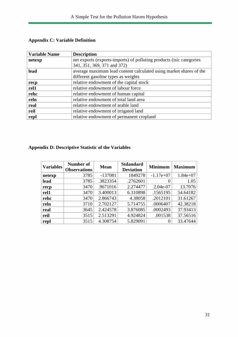
Appendix C: Variable Definition
Variable Name Description netexp net exports (exports-imports) of polluting products (isic categories
341, 351, 369, 371 and 372) lead average maximum lead content calculated using market shares of the
different gasoline types as weights recp relative endowment of the capital stock rel1 relative endowment of labour force rehc relative endowment of human capital reln relative endowment of total land area real relative endowment of arable land reil relative endowment of irrigated land repl relative endowment of permanent cropland
Appendix D: Descriptive Statistic of the Variables
Variables Number of Observations
Mean Stdandard Deviation
Minimum Maximum
netexp 3785 -137081 1849278 -1.17e+07 1.84e+07 lead 3785 .3823354 .2762601 0 1.05 recp 3470 .9671016 2.274477 2.04e-07 13.7076 rel1 3470 3.400013 6.310898 .1565195 54.64182 rehc 3470 2.866743 4.38058 .2012101 31.61267 reln 3710 2.702127 5.714755 .0006407 42.38218 real 3645 2.424578 3.876085 .0002493 37.93413 reil 3515 2.513291 4.924824 .001538 37.56516 repl 3515 4.308754 5.829091 0 33.47644
A Simple Test for the Pollution Haven Hypothesis
32
Appendix E: Preparation of the Lead-Database
The imputation of market shares with missing values followed a two step procedure:
1. Surveys were published every year and contained information on the two most recent
years. This information was used to complete the database as follows:
(a) One year has complete data, one year has missing data: If the market share of
all types of gasoline are missing, the same figures have been taken for both
years. If however only some values are missing, it was assumed that the
missing market shares had the same proportion of the non-missing total as in
the non-missing year.
(b) All values of both years are missing: all market shares are assumed to be
identical.
2. Remaining non trivial patterns of missing values (e.i. some values are missing for both
years): simple interpolation for a given gasoline type was done based on the whole time
period. When no clear time pattern can be observed, the market share was assumed to be
constant with respect to the closest year.
Finally, as data is characterized by a time overlap, only the least recent year from each survey
has been kept, assuming they are more likely to be updated and thus more reliable.

A Simple Test for the Pollution Haven Hypothesis
33
Appendix F: Panel Statistic
Variables Mean Standard Deviation
Minimum Maximum Number of Observations
lead overall .3823354 .2762601 0 1.05 N = 3785 between .2192451 .0008663 .84 n = 62 within .1719442 -.1704995 .9866575 T-bar = 61.0484 recp overall .9498284 2.255159 2.04e-07 13.7076 N = 3540 between 2.180139 2.77e-07 10.96848 n = 57 within .4745689 -3.344543 5.560019 T-bar = 62.1053 rel1 overall 3.727832 6.724835 .1565195 54.64182 N = 3540 between 6.294225 .1789423 30.64262 n = 57 within 2.490936 -10.995 27.72703 T-bar = 62.1053 rehc overall 3.066917 4.596006 .2012101 31.61267 N = 3540 between 4.369906 .2382284 17.96533 n = 57 within 1.611156 -5.283444 16.71425 T-bar = 62.1053 reln overall 2.764517 5.667744 .0006407 42.38218 N = 3805 between 6.501227 .0011022 37.01238 n = 65 within .9430019 -3.687531 11.46999 T-bar = 58.5385 real overall 2.603697 4.012287 .0002493 37.93413 N = 3740 between 5.346093 .0007271 34.79903 n = 64 within .9683346 -3.951542 13.32048 T-bar = 58.4375 reil overall 2.887009 5.563285 .001538 37.56516 N = 3610 between 5.474963 .0024181 31.74753 n = 62 within 1.067978 -5.203308 9.472484 T-bar = 58.2258 repl overall 4.346591 5.92741 0 33.47644 N = 3610 between 6.721187 .0024809 30.92823 n = 62 within 1.693379 -5.109624 18.18694 T-bar = 58.2258 netexp overall -134164.2 1826588 -1.17e+07 1.84e+07 N = 3880 between 793117.8 -2409670 2798806 n = 66 within 1657978 -1.02e+07 1.55e+07 T-bar = 58.7879