NOT FOR QUOTATION WITHOUT PERMISSION OF THE AUTHOR

A SIMPLE MODEL OF THE ECONOMIC LONG WAW

John D. Sterman

April 1985 CP-85-21

Collaborative Papers repor t work which has not been performed solely at the International Institute fo r Applied Systems Analysis and which has received only limited review. Views o r opinions expressed herein do not necessarily represent those of the Insti- tute, i ts National Member Organizations, o r other organizations supporting the work.

INTERNATIONAL INSTITUTE FOR APPLIED SYSTEMS ANALYSIS 2361 Laxenburg, Austria

A summary of this paper w a s presented at the IIASA/IRPET Conference on Long-Waves in Siena/Florence in October 1983. I t w a s not included in the pub- lished proceedings (CP-85-9) of that Conference as w e decided to publish i t separately.

There are several reasons fo r this. First the paper presents, in concise form, the essence of an important school of thought on long-waves which is based on the model described therein. Second, this model depicts the dynam- ics of many microeconomic factors which are important f o r practice and therefore i t comes closest to the business community (recently, even in t h e . form of business games).

From the classification suggested by the authors of this model i t can be labelled as an endogenous, structural (not correlative), and disequilibriurn/dynamic one.

W e hope that the paper wi l l m e e t with interest among not only the research community, but also policy makers in industry.

Boris Segerstahl Deputy Director

iii

A SMPI;E MODEL OF THE ECONOMIC LONG W A ~ '

John D. Stexman

Recent economic events have revived interest in the economic long wave o r Kondratiev cycle, a cycle of economic expansion and depression lasting about fifty years. Since 1975 the System Dynam- ics National Model has provided an increasingly rich theory of the long wave. The theory revolves around "self-ordering" of capital, the dependence of the capital-producing sectors of the economy, in the aggregate, on their own output. The long-wave theory growing out of the National Model relates capital investment, employment and workforce participation, monetary and fiscal policy, inflation, pro- ductivity and innovation, and even political values. The advantage of the National Model is the rich detail in which economic behavior is represented. However, the complexity of the model makes it difficult to explain the dynamic hypothesis underlying the long wave in a con- cise manner.

This paper presents a simple model of the economic long wave. The structure of the model is shown to be consistent with the princi- ples of bounded rationality. The behavior of the model is analyzed, and the role of self-ordering in generating the long wave is deter- mined. The model complements the National Model by providing a representation of the dynamic hypothesis that is amenable to formal analysis and is easily extended to include other important mechan- isms that may influence the nature of the long wave.

INTRODUCTION Recent events have revived interest in the economic long wave, sometimes

known as the Kondratiev cycle, a c cle of economic expansion and depression of approximately fifty years' duration.' Most students of the subject date the troughs of the cycle as the 1830s, 1870s-1890s. 1930s and possibly the 1980s .~ Originally proposed by Van Gelderen, De Wolff, and Kondratiev (Van Duijn 1983), early long-

%his w o r k is based on a model o r ig ina l ly developed i n 1979. I am Indebted t o Dana Meadows, Dennis Meadows, J o r g e n Randers, Leif Ervlk, and Elleabeth Hlcke f o r a s s i s t a n c e w i t h t h e 1979 vers ion , and t o t h e Cruppen f o r Ressurss tud ie r , Oalo, f o r its hospi tal l ty . This r e s e a r c h w a s supported i n p a r t by t h e Sponsors of t h e S y s t e m Dynamlcs National Model Pro jec t . All e r r o r s a r e mine.

2 ~ o n d r a t i e v (1935) remains t h e c l a s s i c of e a r l y long-wave research . Van Dul Jn (1983) pro- v i d e s a comprehensive s u r v e y and a n a l y s i s of long-wave t h e o r i e s and empir ical evidence. A good overv lew of e a r l y long-wave w o r k and a sampllng of r e c e n t work a l so provided by t h e August and October 1981 fiturns 13(4,5), ed i ted by Chr i s topher Freeman; Freeman et al. (1982) focus on unemployment and innovation.

3~ong-wave da t ing is necessar i ly imprec i se due t o t h e l a c k of rel iable data . Van DuiJn (1977) and (1981).

wave work w a s b a e d primarily on the detection of long cycles in economic time series.

Early theories of long cycles stressed w a r and monetary factors such as gold discoveries as causal factors (Tinbergen 1981). Until modern times, Schumpeter's (1939) long-wave theory was the mos t complete and revolved .around i n n ~ v a t i o n . ~ After languishing in the postwar era , the late 1970s witnessed the emergence of long-wave theories based on innovation (Delbeke 1981; Mensch et al. 1981; Mensch 1979), labor dynamics (Freeman 1979; Freeman et al. 1982), resource scarcity (Rostow 1978, 1975), and capital accumulation and class struggle (Mandel 1981, 1980). As Ernest Mandel (1981, p. 332) notes,

It is amusing that the long waves of capitalist development also produce long waves in the credibility of long-wave theories, as well as additional long waves of these theories themselves.

Y e t despite the revival of interest, most economists reject the idea of the long wave. The existence of at most four cycles and the lack of reliable data f o r mos t of that period hamper empirical studies. Most important. neoclassical theory is unable to aocount f o r a disequilibrium mode of behavior with a period of half a century. In the absence of formal. testable theories of the long wave, economists have correctly remained skeptical.

Since 1975 the System Dynamics National Model has provided an increasingly rich theory of the long wave (Forrester 1981, 1979, 1977. 1976; Graham and Senge 1980; Senge 1982). As discussed below, the core of the theory is the "self- ordering" of capital by the trapital sector of the economy: the dependence of capital-producing industries, in the aggregate, on their own output. But the long- wave theory growing out of the National Model is not monocausal: i t relates trapital investment, employment and work force participation, aggregate demand, monetary and fiscal policy, inflation, debt, innovation and productivity, and even political values. The advantages of the National Model are its wide boundary and the rich detail in which economic behavior is represented. However, the complexity of the model and the lack of published documentation make it difficult to explain the dynamic hypothesis underlying the long wave in a simple and convincing manner.

This paper presents a simple model of the economic long wave based on the self-ordering hypothesis. The model demonstrates that self-ordering oan account fo r long waves, and isolates the minimum structure sufficient to generate a long wave. In addition, the paper stresses the role of bounded rationality in generating the long wave. I t is shown that the decision rules represented in the model f o r managing production, investment, and so on are Looally rational. However, when interacting in the context of the system as a whole. they produce "imtional" behavior: periodic over- and under-expansion of the economy.

THE DYNBMC HYPOTHESIS: SELF-OBDERING This section outlines the dynamic hypothesis of self-ordering and sketches a

conceptual model illustrating the most important mechanisms that contribute t o the long wave.5 Consider the economy divided into t w o sectors: the capital sector and the goods sector. The capital-producing industries of the economy (the construc- tion, heavy equipment, steel, mining, and other basic industries) supply each other with the capital plant, equipment, and materials each needs to operate. Viewed in

%he renaieeance o f interes t i n Schumpeter'e claeeic work (1939) i e i l lustrated in, e.g., Van Duijn (1981), Menech et al. (1981), and Kleinknecht (1981).

5 ~ h e notion of a dynamic hypotheeie ie diecussed by Randere (1980).

the aggregate, the capital sector of the economy orders and acquires capital from itself, hence "self-ordering ".

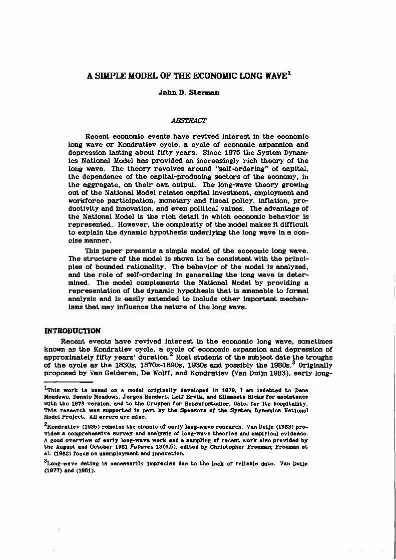
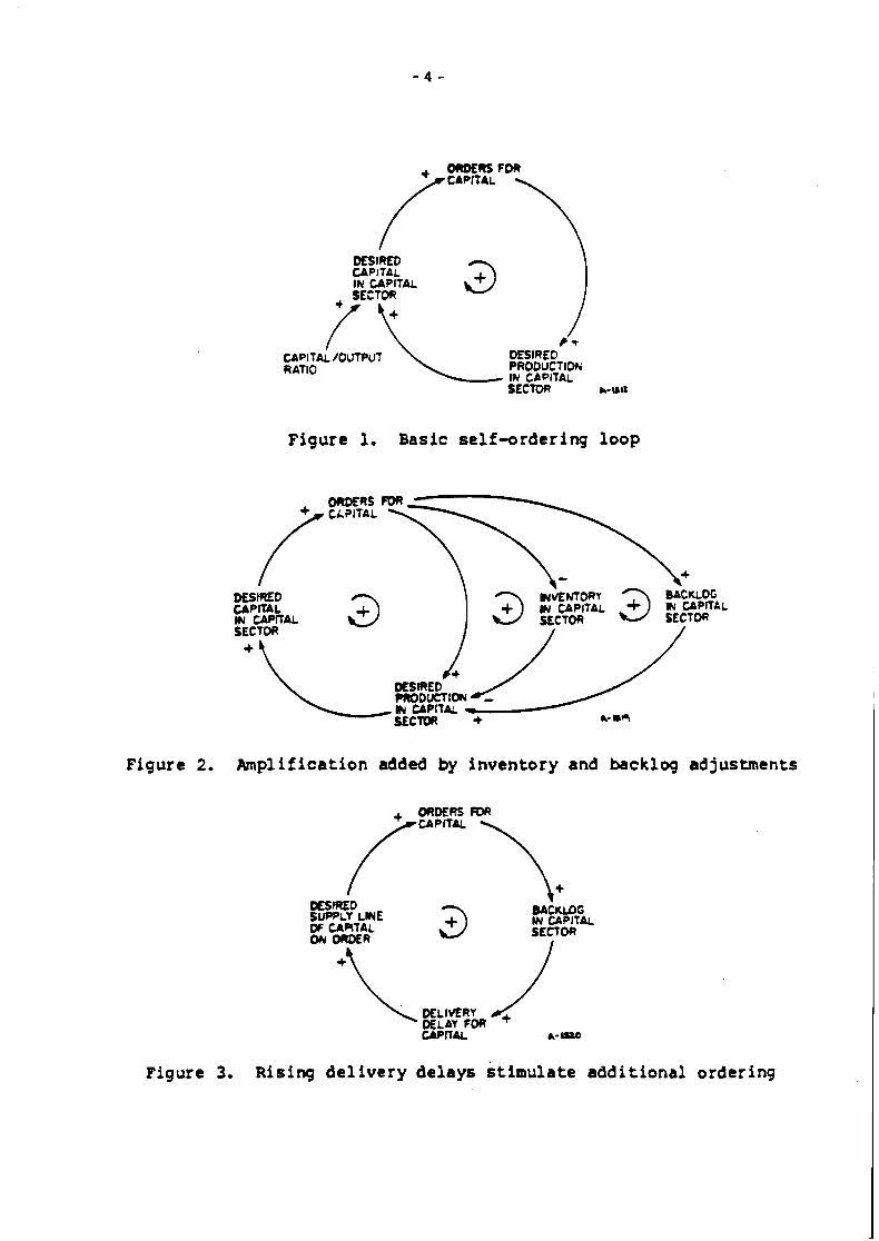
If the demand for consumer goods and services increases, the consumer-goods industry must expand its oapacity and so places orders f o r new factories, equip- ment, vehicles, etc. To supply the higher volume of orders, the capital-producing sector must also expand its capital stock and hence places orders f o r more build- ings, machines, rolling stock, trucks, etc., causing the total demand f o r capital to r ise still further , a self-reinforcing spiral of increasing orders, a greater need f o r expansion, and still more ~ r d e r s . ~

Figure 1 shows the most basic positive feedback loop created by self- ordering. The strength of the self-ordering feedback depends on a number of fac- tors, but chiefly on the capital intensity (capital/output ratio) of the capital- producing sector. A rough measure of the strength of self-ordering can be calcu- lated by considering how much oapital production expands in equilibrium in response to an increase in investment in the rest of the economy.

Production of capital equals the investment in plant and equipment of the goods sector plus the investment of the capital sector:

KPR =Grn+MNV (1)

where

KPR = Capital sector, production (capital units/year)

GINV = G o o d s sector, investment (capital units/year)

MNV = Capital sector, investment (capital units/year)

In equilibrium, investment equals physical depreciation. If the average life- t ime of capital (the aggregate of plant and equipment) were twenty years, one- twentieth of the capital stock would have to be replaced each year. Thus

where

KC = Capital sector, capital stock (capital units)

U C = Capital sector, average life of capital (years)

The capital stock KC is related to capital production KPR by the capital/output rat io KCOR (years):

Substituting for KINV and KC yields

Equation 4 indicates how much capital production must increase in the long run when the investment needs of the rest of the economy rise, taking into account the ex t ra capital needed to maintain the capital sector's own stock at the higher level.

'self-ordering is closely related to the investment accelerator, which i s commonly thought to be a factor in the 4- to 7-year business cycle. However, recent work as well as classics such as Metzler (1941) indicate the business cycle revolves around inventory management and suggest the accelerator i s primarily involved in longer modes (Forrester 1982; Low 1980; Mass 1975).

DESIRED CAPITAL IN CAPITAL SECTOR .v

cn~~mi /OUTPUT RATIO

DESIRED- PRODUCT IOH IN CAPITAL SECTDR

Figure 1, Basic se l f -ordering loop

DESIRED BACKLOG CAPITAL Ih' CAPITAL MI CAPITAL SECTDR

+ 4

Figure 2. Amplification added by inventory and backlog adjustments

#SIRED 1

SUPPLY LME w CAAtAL

EE%'FiL ON ORDER SECTOFl

I

Figure 3, Rising d e l i v e r y delays s t imulate addit ional ordering

Assuming an avemge life of capital of twenty years and an average capital/output rat io of three years (approximate values for the aggregate economy), the expres- sion above yields a multiplier effect of 1.18: in the long run, an increase in invest- ment in the rest of the economy yields an additional 16% increase in total invest- ment through self-ordering .

The long wave is an inherently disequilibrium phenomenon, however, and dur- ing the transient adjustment to the long run the strength of self-ordering is greater than in equilibrium. As shown in Figure 2, an increase in orders fo r capi- tal not only increases the steady-state rate of output required, but, because pro- duction of capital lags behind orders, depletes the inventories and s w e l l s the back- logs of the capital sector. To correc t the imbalance, firms must expand output above the order ra te , causing desired capital to expand further, and further swel- ling the total demand fo r capital. Production m u s t remain above orders long enough to restore inventories and backlogs to normal levels.

Production Lags behind orders fo r several reasons. I t takes t ime for firms to recognize that an unanticipated change in demand is permanent enough to warrant a change in output. And once desired output rises, it takes time to increase employment and especially to increase capacity.

The disequilibrium pressures of low inventory and high backlog can signifi- cantly amplify the effect of an unanticipated change in demand, further strengthening the basic self-ordering loop.7 Other mechanisms create additional amplification: when orders fo r capital exaeed production, delivery t imes begin to rise. Faced with longer lead times and spot-shortages of specialized equipment, firms must hedge by ordering far ther ahead and placing orders with more than one supplier, a process described by Thomas W. Mitchell in 1923 (p.645):

Retailers find that there is a shortage of merchandise at their sources of supply. Manufacturers inform them that it is with great regret that they are able to fill the i r orders only to the extent of 80 p e r cent; there has been an unaccountable shortage of materials that has prevented them from producing to their full capacity. They hope to be able to give full service next season, by which time, no doubt, these unexplainable condi- tions will have been remedied. However, retailers, having been disap- pointed in deliveries and lost 20 p e r cent o r more of their possible pro- fits thereby, are not going to be caught that way again. If they want 90 units of an article, they o rder 100 so as to be sure. each, of getting the 90 in the p ro rata share delivered. Probably they are disappointed a second t ime. Hence they increase the margins of their orders over what they desire, in o rder that the i r p ro rata shares shall be fo r each the full 100 p e r cent that he really wants. Furthermore, to make doubly sure, each merchant spreads his orders over more sources of supply.

The hoarding phenomenon described by Mitchell is quite common, m o s t recently contributing to the gasoline crisis of 1979 (Neff 1982).

For the aggregate capital sector, however, ordering far ther ahead to com- pensate for a rising lead time adds to the total demand fo r capital, causing lead t i m e s to rise still further and creating still more pressure to order (Figure 3).

Other sources of amplification include growth expectations - the spread of optimism and pessimism - as described by Wesley Mitchell (1941, p.5):

Virtually all business problems involve elements that are not precisely known, but must be approximately estimated even fo r the present, and

7 ~ a a s (1980) discusses amplification created by stock-and-flow disequilibrium.

forecast still more roughly f o r the future. Probabilities take the place of certainties, both among the data upon which reasoning proceeds and among the conclusions at which it arrives. This fact gives hopeful or despondent moods a large share in shaping business decisio ns... M o s t men find their spirits raised by being in optimistic aompany. Therefore, when the f i rs t beneficiaries of a t rade revival develop a cheerful frame of mind about the business outlook, they become centers of infection, and start an epidemic of optimism.

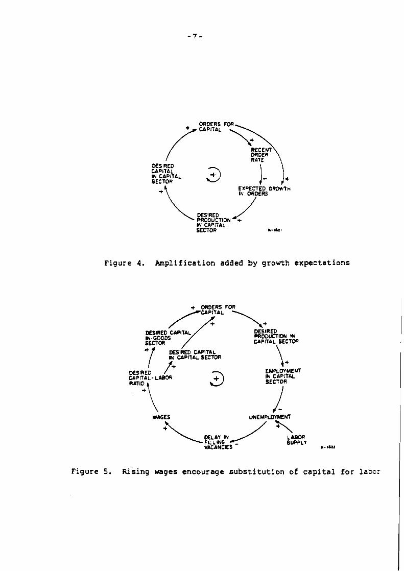
To the extent expectations of future growth lead to expansion of investment, self-ordering ensures the demand for capital wi l l in fact rise, validating and strengthening the forecast of continued growth (Figure 4).

Interactions with the labor market further strengthen self-ordering (Figure 5). To boost output, the capital sector expands employment as w e l l as its capital stock. As the pool of unemployed is drawn down, the labor market tight8.m and wages rise. Scarcity of skilled workers and higher Labor costs encourage the sub- stitution of capital for labor throughout the economy, fur ther augmenting the demand for capital. Thus one would expect the early phases of a long wave to involve expansion of labor and capital together, followed by a period of stagnant employment but continued growth in capital and output. Such patterns emerge f r o m simulations of the National Model and have been documented for both the US, Europe. and Japan (Freeman 1979; Freeman et al. 1982; Graham and Senge 1980; Senge 1982).

Still more amplification is due to interactions w i t h the financial markets (Fig- ure 6). Rising oapital demand boosts priaes and profitability, leading to expansion of existing firms and the entry of new firms. In addition, the expansion of the asset and earnings base of the capital sector increases the external financing available f o r expansion. I t is through these channels that monetary policy wi l l influence the long wave, by providing (or withholding) credit sufficient to finance the demand for investment. Further amplification can be added if. as investment slows near the peak of a long wave. the monetary authority expands credit and lowers interest rates in an effort to buoy up the boom.'

Additional amplification arises f r o m the familiar consumption multiplier: the expansion of the capital sector's output and employment boosts aggregate income, which feeds back to fur ther stimulate investment demand by augmenting the demand fo r consumer goods and housing (Figure 7).

Interactions between self-ordering and innovation, international trade, and political values also exist and may further amplify the long wave.'

According to the theory derived from the National Model, the net effect of the positive feedback loops described above is to significantly amplify the basic self- ordering loop. Once a capital expansion gets under way, these loops sustain it until production catches up to orders, excess capital is built up, and orders begin to fa l l . A t that point, the loops reverse: a reduction in orders further reduces investment demand, leading to a contraction in the capital sector's output and dec- lining employment, wages, aggregate demand. and output. Capital production must remain below the level required for replacement and long-run growth until the

' ~ o n e t a r y stimulus in the latter phases of the long-wave expansion may account in part for the historic movement of aggregate prices over the long wave.

innovation, see the work of Mensch and Freeman. Content analysis of political plat- forms has documented 50-year cycles in both American and British political values that correspond t o the timing of the economic cycle (Narnenwirth 1973; Weber 1981).

DESIRED CAPITAL IN CAPITAL SECT OR

+ f EXDECTED GR&TH Ih' ORDERS

PRODUCTION + # CAPITAL SECTOR h- UL I

Figure 4. Amplification added by growth expectations

CAPITAL SECTOR

DESIRED f MPLWMENT CAPITAL- LABOR IN CAPITAL

WAGES UNEMPLMHEN~

Figure 5. Rising wages encourage substitution of capital for lab=:

DESIRED CAPITAL IN CAPITAL SECTOR

+i ENTRY AND EXPANSION

BACKLOG IN CAPITAL SECTOR

DE; I V E W Df LA' FOR CAPli&L

SECT OR A- 1 ~ 2 %

Figure 6 . Ris ing return encourages e n t r y and expansion

DESIRED CAPITAL IN GOODS SECTOR

DESIRED PRODUCTIDh' IN GOODS SECTOR s

+ I/ AGGREGATE + INCOME

Figure 7 . Amplif icat ion added by feedback through- aggregate demand

excess physical and financial capital is depreciated - a process that may take a decade o r more due to the long lifetimes of plant and equipment. Once the capital stock is worn out, investment rises, triggering the next upswing.

F i r e 8 shows a typical series of long waves generated by the National model. The simulation exhibits the short-term (4- to 7-year) business cycle as well as a 48- to 56-year long wave. Several features of the simulation bear com- ment:

1. The long wave is strongest in the capital sector, while the goods sector is relatively unaffected.

2. Capital stock in the capital sector peaks af ter production (due to con- struction delays) and declines slowly, depressing capital production.

3. The delivery delay fo r capital peaks before the peak of production.

The preceding discussion does not comprise a complete model of the long wave. Many important relationships have been omitted. Rather, the relationships above constitute a dynamic hypothesis - the essential feedback structure believed to be important in the genesis of the long wave. To be a useful hypothesis, the importance of self-ordering must be evaluated in a formal model that permits reproducible tests to be made. Further, the relative importance of the various self-ordering loops must be evaluated. The model developed below is used to address the following questions:

1. Is self-ordering sufficient to produce a long wave? 2. What factors control the period and amplitude of the long wave?

3. What nonlinearities are important in causing the long wave?

4. How might mechanisms excluded from the model alter its behavior?

BOUNDED BATIONALITY Before proceeding to the model, this section reviews the behavioral underpin-

nings of the theory. The model presented below is based in par t on the theory of bounded rationality (Cyert and March 1963; March 1978; Merton 1936; Nelson and Winter 1982; Simon 1947, 1957, 1978, 1979). The essence of the theory is summar- ized in the principle of bounded rationality, as formulated by Herbert Simon (1957, p. 198) :

The capacity of the human mind for formulating and solving complex problems is very small compared with the size of the problem whose solu- tion is required fo r objectively rational behavior in the real world o r even fo r a reasonable approximation to such objective rationality.

The theory of bounded rationality is supported by an extremely large and diverse body of empirical research, which not only documents the limitations of human information processing, but highlights the systematic biases and e r r o r s deeply embedded in the heuristics people use to make decisions. While a complete catalo- gue of bounded rationality in its many guises is beyond the purpose of this paper, those aspects most important fo r theories of economic behavior in general and fo r this paper in particular can be stated quite simply.''

'O~he behavior is triggered by exponentially autocorrelated no ise i n exogenous constuner demand with a t ime constant of 0.25 y e a r s and a standard deviat ion of 2.5% of t h e mean.

l l ~ o m p l e t e re ferences cannot be given here. Excellent discussion and references t o t h e l i t erature can be found i n Kahneman et aL (1982) and Hogarth (1980). Morecroft (1983) provides an excel lent treatment o f t h e relat ionships between bounded rational i ty and eye- tern dynamics. See a lso Dutton and Starbuck (1971).

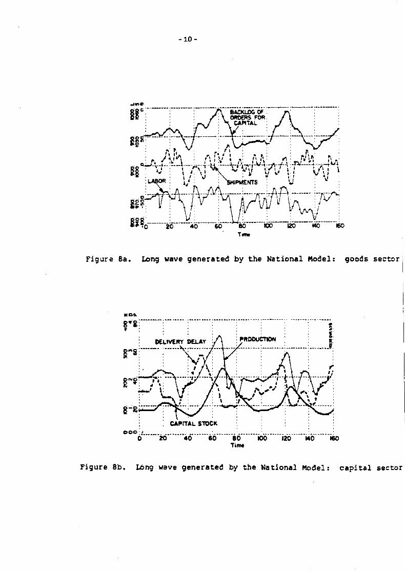
Figure 8a. Long wave generated by the National Model: goods sector i

- ------ .. .- .-- --. -. ----.---- ------.. - - - - - - - --- . --- ---. -. . 000 :L ...-.*..-...-iO &" 8' 0 100 I20 uo I60

Time

Figure 8b. Lbng wave generated by t h e National Model : capital sector

1. Limited Information-Proceging Capability

Humans have a limited ability to process information. As a consequence, "per- ception of information is not comprehensive but selective" (Hogm3.h 1980, p.4; emphasis in original). For both physiological and psychological reasons, people take only a very few factors o r cues into account when making decisions. E'urther, the cues that a r e taken into account are not those with the best predictive ability. Rather people focus on cues they judge to be relatively certain, systematically excluding uncertain o r remote information regardless of its importance (Hogarth 1980, p. 36; Kahneman et al. 1982, esp. Ch. 4, 7-10). Additionally, since "people give more weight to data that they consider causally related to a target object. ..," they focus on cues they believe to be meaningful (Hogarth 1980, p. 42- 43, emphasis in original). However, precisely because of limited information- processing capability and the aversion to unoertainty, people are notoriously poor judges of causality and correlation, and in controlled experiments systematically create mental models at variance with the known situation.12 Ironically, "people tend to believe that they pay attention to many cues, although models based on only a f e w cues can reproduce their judgements to a high degree of accuracy" (Hogarth 1980, p. 48). Though sometimes aware of the pitfalls in judgement and inference, people, including many professionally trained in statistics, consistently assert that their own performances a r e immune, are reluctant to abandon their mental models and selectively use hindsight to "validate" their mental models.13

As a consequence of limited information-processing ability, organizations (and the individuals within them) divide the total task of the organization into smaller units. By establishing subgonls assigned to subunits within the organization, the complexity of the total problem is vastly reduced. The subunits in the hierarchy ignore, o r treat as oonstant or exogenous, those aspects of the total situation that are not directly related to their subgoal (Simon 1947, p.79):

Individual choice takes place in an environment of "givens" - premises that are accepted by the subject a s bases for his choice . . . Limited information-processing ability also forces people within organiza-

tional subunits to evolve simple heuristics o r rules of thumb to make decisions. The rules of thumb rely on relatively certain information that is locally available to the subunit. Rules of thumb are also aomputationally simple (Morecroft 1983, p.133):

In the short run, these procedures do not change, and represent the accumulated learning embodied in the factored decision making of the organization. Rules of thumb need employ only small amounts of informa- tion.. . Rules of thumb process information in a straightforward manner, recognizing the computational limits of normal human decision makers under pressure of time.

Such factoring is central to the management of all but the smallest enter- prises. Indeed, organization, as Simon (1947, p.80) states, "permits the individual

12~ogar th (1980) diecueeee numerous separate eources of biaa i n decision making. Among t h e common fallacies of caueal attribution are t h e gambler's fallacy and t h e regreeeion fallacy. (Tveraky and Xahnsman 1974).

13see Kahnsman et al. (1982), eepecially Ch.2,9-12,20, and 23. Coffman'e (1959) "dramatur- gic" model of public behavior is relevant here: People constantly ad jus t their public per- formance~ 80 ae t o enhance their statue and competence i n the eyes of othere.

to approach reasonably near to objective rationality." The implicit assumption (necessitated by the complexity of the total situation and the limited t i m e available fo r decision making) is that the task is separable in the sense that achieving the subgoals ensures attainment of the larger goal.

THE PODEL The model will be presented in several stages. First, a simplified, generic

model of a firm o r sector of the economy will be developed (the "production sec- tor"). I t wi l l be shown, through partial model tests, that the decision rules for production and investment yield rational behavior in the simplified environment presumed by each subunit of the organization. The model will then be used to represent the aggregate capital-producing sector of the economy, including self- ordering. Finally, simulation experiments will be used to establish the relative contribution of the structural and parametric assumptions to the resulting long- wave behavior. l4

Pt = Bt / NAD (3)

where

P ! = Production rate (units/year)

PC = Production capacity (units/yerrr)

CU = Capacity utilization (fraction)

P = Indicated production (units/year)

B = Backlog of unfilled orders (units)

NDD = Normal delivery delay (years)

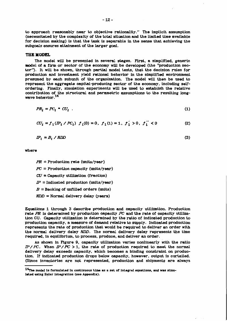
Equations 1 through 3 describe production and capacity utilization. Production rate P ! is determined by production capacity PC and the rate of capacity utiliza- tion CU. Capacity utilization is determined by the ratio of indicated production to production capacity, a measure of demand relative to supply. Indicated production represents the ra te of production that would be required to deliver an order with the normal delivery delay NDD. The normal delivery delay represents the time required, in equilibrium, to process, produce, and deliver an order.

A s shown in Figure 9, capacity utilization varies nonlinearly with the ratio IF /PC. When P/PC > 1 , the rate of production required to meet the normal delivery delay exceeds capacity, which becomes a binding constraint on produc- tion. If indicated production drops below capacity, however, output is curtailed. (Since inventories a r e not represented, p r o d ~ c t i o ~ and shipments a r e always

14T'he model I s formulated In continuoua t ime a s e set of Integral equations, and was simu- lated using Euler integration ( s e e Appendix).

equal, and if there a r e no orders to be filled, production must decline to zero unless one assumes firms simply throw the extra output away.) If firms wanted to maintain the normal delivery delay regardless of capacity, capacity utilization would fall in proportion to the decline in demand, production would equal indicated production, and CU would lie along h e A. If firms wanted to continue to operate at full capacity at all times, even in the face of diminished demand, utilization would fall only when the sector w a s producing at the minimum delivery delay, defined by line B . ' ~ Capacity utilization is specified as a compromise between these two extremes: if indicated production drops below capacity, firms are assumed to reduce utilization only sllghtly, preferring to maintain relatively full utillzation (and hence revenues) by drawing down their backlogs. Delivery delays would become shorter than normal. If backlog continued to fall, utilization would be cut back, but at less than proportional rates, until firms w e r e producing at the minimum delivery delay. Further declines in backlog then force proportional reductions in output. The behavior described by the capacity utilization formula- tion is illustrated by the following description of the machine tool industry &si- nes~ Week. 1 4 March 1982, p.20):

Bad a s they are, shipments are outpacing orders by a very wide margin, forcing a continued rundown in the industry's order backlog ... A t the average shipment rate of the past three months, backlogs provide less than six months of production, in an industry that had a one-year backlog when the recession beg an... the low level of capacity utilization suggests that shipments will run ahead of orders we l l into summer.

where

C = Capital stock (capital units)

COR = Capital/output ratio (years)

Production capacity is determined by capital and the capital/output ratio. For simplicity, capital is the only explicit factor of productlon, and the capital/output ratio is assumed fixed, implicitly assuming other factors (particu- larly labor) are freely available.16

15Line B de te rmines t h e minimum d e l i v e r y delay because t h e a c t u a l d e l i v e r y de lay o r a v e r a g e res idence t i m e of a n o r d e r i n t h e backlog is given by Ll)iB/F?ZiB/ W W ) . When W=b*(P/FC) f o r b > 1 and b a ( I P / R ) 61, 1.9. when CU U e s along l i n e B a D e / (PC.b(IP/R))=B/ (baIP) but IP=B/hW, a o I#)=B/ (baB/hEkD)=hEkD/ b = m where YID - Minimum d e l i v e r y de lay (years).

1 6 ~ h o u g h a more complete model would include a more sophis t i ca ted production funct ion w l t h both v a r i a b l e labor and a v a r i a b l e w o r k week, t h e dynamics of l abor acquisi t ion a r e p r imar i ly assoc ia ted w l t h t h e shor t - t e rm business cyc le (see foo tno te 6). However, s i n c e r i s i n g wages c o n t r i b u t e t o t h e s t r e n g t h of self-ordering during a long-wave expansion (Figure 5). omission of l abor a s a n e x p l i c i t f a c t o r is Ukely t o reduce t h e model's a b i U t y t o g e n e r a t e a long wave. F o r a dynamic model w l t h multiple f a c t o r s of production t h a t con- f o r m s t o t h e pr inciples of bounded r a t i o n a U t y see Sterrnan (1981, 1982).

INDICATED PRODUCTION IP NSIONLESS, PRODUCTION CAPACITY PC

Figure 9 . Capacity u t i l i z a t i o n

INDICATED CAPITAL ORDER FRACTION ICOF ( FRACTION /YEAR h- rUc

Figure 10. Capital order f rac t ion

where

CA = Capital acquisitions (capital units/year)

W = Capital discards (capital units/year)

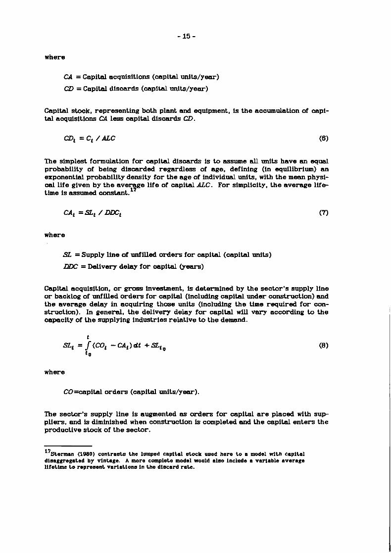
Capital stock, representing both plant and equipment, is the accumulation of capi- tal acquisitions CA less capital discards W.

The simplest formulation for capital discards is to assume all units have an equal probability of being discarded regardless of age, defining (in equilibrium) an exponential probability density for the age of individual units, with the mean physi- cal life given by the a v e y e life of capital ALC. For simplicity, the average l i f e time is assumed mnstmt. l

where

SL = Supply line of unfilled orders for capital (capital units)

= Delivery delay for oapital (years)

Capital acquisition, o r grass investment, is determined by the seator's supply line o r backlog of unfilled orders for capital (including capital under construction) and the average delay in acquiring those units (including the time required for con- struction). In general, the delivery delay for capital w i l l vary according to the capacity of the supplying industries relative to the demand.

where

CO=capital orders (capital units/year).

The sector's supply line is augmented as orders for capital are placed with sup- pliers, and is diminished when construction is completed and the capital enters the productive stock of the sector.

17~termsn (1980) contrade the lumped capital dock used here to a model wi th capital disaggregated by vintage. A more complete model would also include a variable average lifetime to represent variations i n the discard rate.

where

CQYP = Capital order fraction (fraction/yeetr)

I C W = Indicated capital order fraction (fraction/year)

CC = Correction to orders from capital stock (capital units/year)

CSL = Correction to orders from supply line (capital units/year)

Though capital acquisition oorresponds to investment, it is the order rate for capital that determines acquisitions. Three motivations for ordering capital a r e assumed: First, to replace discards; second, to correct any discrepancy between the desired and actual capital stock; and third, to correct any discrepancy between the desired and actual supply line. l8 The sum of these three pressures, as a fraction of the existing capital sbuk . defines the indioated capital order frac- tion ICQYP. However, in extreme c i r c ~ c e s the indicated capital order frac- tion may take on unreasonable values. For example, an extreme exoess of capacity could cause I C W to be negative. A s shown in Figure 10, the actual order fraction COF is a nonlinear function of the indioated order fraction. Since gross investment must be positive, COF asymptotically approaches zero as I C W drops below 5% year." Similarly, if demand f a r exceeds capacity, the indicated order fraction may take on unreasonably large values. I t is assumed that the Wimum capital order fraction is 30% of the capital stock per year. The l imit reflects physical constraints to rapid expansion such as labor and materials bottlenecks, financial constraints, and organizational pressures .20

1 8 ~ n v e e k w n t r e s u l t i n g f r o m growth e x p e c t a t i o n s would have t o be included i n a more corn- p l e t e model. The inves tment funct ion of t h e model is a simplified v e r s i o n o f t h e S y s t e m Dynamics National Model invea tment funct ion. Senge (1978,1980) s h o n e t h e SDNM funct ion reduces t o t h e neoclassical i n v e s k a e n t funct ion (e.g. Jorgenson 1963; Jorgenson ct UL 1970) when a v a r i e t y of equilibrium and p e r f e c t information assumptions are made. The SDNM funct ion is shown t o p rov ide a b e t t a r atatistical flt of invee tment d a t a and t o behave more plausibly t h a n t h e neoclassical funct ion when faced wi th v a r i o u s test inputs .

he formulat ion f o r COF exc ludes o r d e r canceIlations. Disallowing cancel lat ions is a s implifying assumption. A more complete model would d i saggrega te unfilled o r d e r s f r o m u n i t s under cons t ruc t ion and would r e p r e s e n t cancel lat ions e x p l i c i t l y (Sterman 1981). The formulat ion f o r CYF amoothly approaches s e r o d u e t o t h e aggregat ion of firms, some of which wlll be order ing nonaero amounts even when t h e a v e r a g e ICCF < 0. The va lues of C W f o r ICQF < 0.05 w e r e es t imated by assuming (1) t h e order ing funct ion of a mingle f l r m is CtF = IULY(0JCOT) and (2) ICQF f o r t h e aggrega te s e c t o r is d i s t r i b u t e d normally w i t h a v a r i a n c e of O.O5/year. 20

The va lues of C W f o r ICQF S 0.05 w e r e der ived by assurnlng t h e o r d e r funct ion of an indi- vidual f i r m w a s lKN(0.30JCQF) and t h a t ICQF is d i s t r i b u t e d normally wi th a v a r i a n c e of O.O5/year.

D L , = mt * PDm,

where

M'L = Desired supply line (capital units)

TASt = Time to adjust supply line (years)

PDDC = Perceived delivery delay for capital (years)

Dm = Delivery delay for capital (years)

Equations 12 through 14 describe the management of the supply line. Firms strive to eliminate discrepancies between the desired and actual supply line within the time to adjust supply line TASL. To ensure an appropriate acquisition rate, firms must maintain a supply line proportional to the delivery delay they face in acquiring capital: as described by Mitchell (1923). if the delivery delay rises, firms must plan for and order new capital farther ahead, increasing the required supply line. The desired supply line is based on relatively certain information: the discard rate and the delivery delay for capital perceived by the firm. For sim- plicity, delays in perceiving the m e lead time for capital are not represented, thus the perceived delivery delay for capital is assumed to equal the actual delivery delay. However, the relationship between delivery delay and the desired supply line is likely to be highly nonlinear: as Mitchell notes, initially a change in delivery delay may produce a more than proportional change in orders due to hoarding and panic. And rather than expand orders continually as lead times rise, chronically high delivery delays would eventually cause firms to seek substitutes, limiting the desired supply line. The sensitivity of the model to the decision rule for desired supply line is tested below.

CCt = (DCt - Ct ) TAC (15)

ICt = I . : * COR (17)

where

DC = Desired capital (capital units)

TAC = Time to adjust capital (years)

RC = Reference capital (capital units)

IC = Indicated capital (capital units)

E.= Indicated production capacity (units/year)

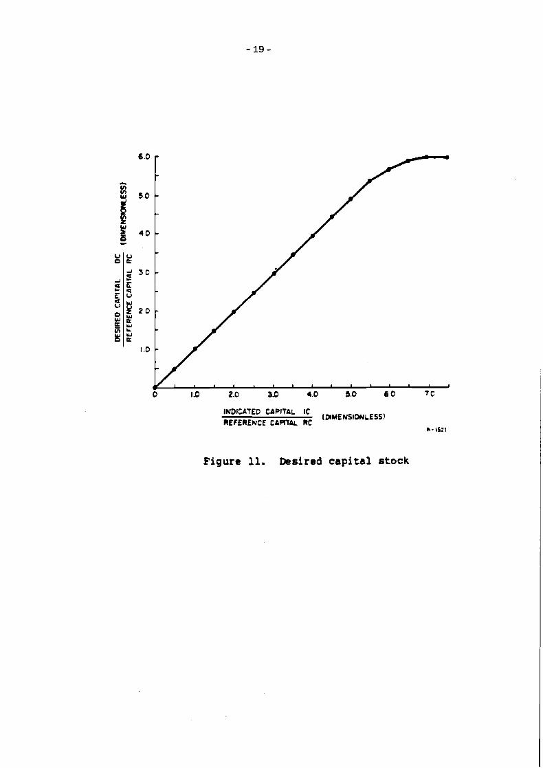
Equations 15 to 17 describe the adjustment of capacity to desired levels. Like the supply U e correction, firms attempt to correct discrepancies between desired and actual capital stock over a period of time given by the time to adjust capital. Desired capital is nonlinearly related to the indicated capital stock, which is the stock needed to provide the indicated production capacity I E . (Indicated produc- tion capacity is the capacity judged necessary to m e e t expected demand.) As shown in Figure 11, diminishing returns to uapital are assumed to set in when IC becomes large relative to a referenae level of capital RC (set at the initial eqnili- b r i m of the system). Though labor is not explicitly represented, the linear range of the relationship between IC and PC implies employment can be expanded in pr* portion to capital. As the available labor supply is exhausted, however, further expansion of capital lowers the marginal productivity of capital and diminishes incentives for further expansion even if demand remains high.

CBt = (Bt - IBt ) / TAB (19)

where

EO = Expected orders (units/year)

CB = Correction from backlog (units/year)

LB = Indicated backlog (units)

TAB = Time to adjust backlog (years)

Equations 18 through 20 determine indiaated production capacity. I t reflects the capacity the sector judges necessary both to fill expected orders EO and adjust the backlog of unfilled orders to an appropriate level. The speed with which the sector strives to correct discrepancies between the actual and indicated backlog is determined by the time to adjust backlog, a reflection of the sector's sensitivity to abnormal delivery delays. Indicated backlog is the backlog that would be neces- sary to fill the expected order rate within the normal delivery delay.

OR, - EO, = J TAO

t 0

where

TAO = Time to average orders.

INDICATED CAPITAL IC (DMENSIDIJLESS) REFERENCE CAPITAL RC

Figure 11. Desired capi ta l stock

The expected order rate represents the sector's forecast of demand condi- tional on available information and the rules of thumb for forecasting used by the sector. The firm is assumed to forecast demand by averaging past orders. Orders a r e averaged because i t takes time for firms to decide that an unanticipated change in demand is lasting enough to warrant capacity expansion. The averaging serves to filter out short-term noise in demand, providing a more certain measure of long-run demand than the r a w order rate, and preventing wild swings in invest- ment by allowing the backlog to buffer the system from the short-term variability of demand. First-order exponential smoothing is assumed fo r the averaging pro- cess. The smoothing time is given by the time to average orders TAO."

ORt = exogenous (24)

Finally, the delivery delay for the sector's output, o r average residence time of an order in the backlog, is given by the rat io of backlog to production. The backlog of unfilled orders accumulates orders less shipments (production). The order ra te is assumed exogenous; delivery delay fo r capital is exogenous and assumed constant.

The parameter values assumed for the analysis are summarized in Table 1. The parameters were chosen to represent a producer of capital goods. The param- eters a r e broadly consistent with survey and econometric evidence reported in various studies. But because the model excludes all but the most basic channels through which self-ordering operates, precise estimation is not warranted. The sensitivity of the model to the key parameters is analyzed below.

THE LOCAL EATIONALWY OF THE DECISION BUMS The behavioral formulations in the model conform to the principles of bounded

rationality: management of the firm is broken down into several distinct decisions (production, investment, demand forecasting, etc.). The individual decision rules rely on locally available, relatively certain information. For example, desired production capacity relies on the backlog and average orders ra ther than the current and less certain order rate. Similarly, the desired supply line requires knowledge only of the replacement ra te of investment and the delivery delay for capital experienced by the firm, and does not consider the condition of capital suppliers o r the effect demand changes might have on availability. Simple rules of thumb are used to determine how much capital to keep on order, how fast to adjust production capacity, and how to manage backlogs. To test the local o r intended rationality of the decision rules, this section describes partial mode l tests of the

'krowth expectation8 would have t o be included in a more complete model of demand fore- casting, and would add amplification.

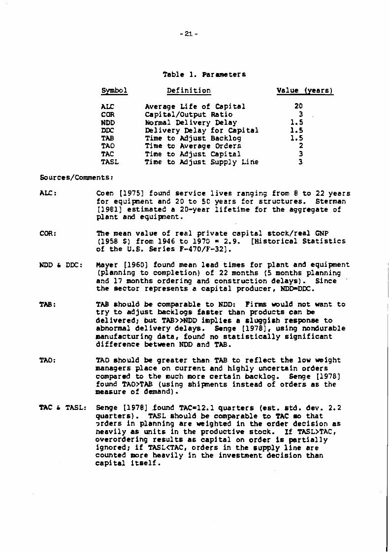
Table 1. Parameters

&!!EL Def in i t ion Value (years)

AU: COR NDD DDC TAB TAO TAC TASL

Average Life of Capi ta l Capital/Output Ratio Normal Delivery Delay Delivery Delay f o r Cap i t a l Time t o Ad j u s t Backlog Time to Average Oreers Time t o M j u s t Capi ta l Time to M j u s t Supply Line

A I L : Coen [I9751 found s e r v i c e l i v e s ranging from 8 t o 22 yea r s f o r equipment and 20 t o 5C years for s t r u c t u r e s . Sterman [1981] est imated a 20-year l i f e t i m e f o r the aggregate of p l a n t and equipnent.

COR: The mean value of r e e l p r i v a t e c a p i t a l s tock / rea l GNP (1958 $) from 1946 t o 1970 = 2.9. [His to r i ca l S t a t i s t i c s of t h e U.S. S e r i e s F-470/F-321.

NDD & DDC: Mayer [1960] found mean lead times f o r p l a n t and equipment (planning t o completion) of 22 months ( 5 months planning and 17 months ordering and cons t ruc t ion d e l a y s ) . Since .

t h e s e c t o r r ep resen t s a c a p i t a l producer, NDD=DDC.

TAB : TAB should be comparable t o NDD: Firms would not want t o t r y t o a d j u s t backlogs f a s t e r than products can be del ivered; but TAB>>NDD implies a s lugg i sh response t o abnormal d e l i v e r y delays. Senge [1978], using nondurable manufacturing d a t a , found no s t a t i s t i c a l l y s i g n i f i c a n t d i f f e r e n c e between NDD and TAB.

TAD should be g r e a t e r than TAB t o r e f l e c t t h e low weight managers p lace on c u r r e n t and h ighly uncer ta in o rde r s compared to t h e much more c e r t a i n backlog. Senge [1978] found TAO>TAB (using sh ipnen t s ins tead of o r d e r s a s the measure of demand).

TAC & TASL: Senge [I9781 ,found TAC=12.1 q u a r t e r s (est. s t d . dev. 2.2 q u a r t e r s ) . TASL should be comparable t o TAC so t h a t 2 rde r s i n planning a r e weighted i n t h e order decis ion a s neavi ly as u n i t s in the productive s tock. If TASLBTAC, overordering r e s u l t s as c a p i t a l on o rde r is p n r t i a l l y ignored; i f TASL<TAC, o r d e r s in t h e supply l i n e a r e counted more heavi ly i n the investment dec i s ion than c a p i t a l i t s e l f .

production and investment decisions. A minimum requirement for intended rationality is that the individual decision rules respond wel l to shocks when the decision rules are tested in isolation.

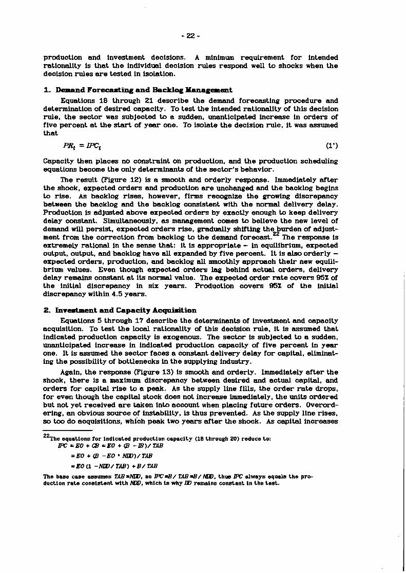
1. Demand Forecasting and Backlog Management Equations 18 through 21 describe the demand forecasting procedure and

determination of desired capacity. To test the intended rationality of this decision rule, the sector w a s subjected to a sudden, unanticipated increase in orders of five percent at the start of year one. To isolate the decision rule, it w a s assumed that

Capacity then places no constraint on production, and the production scheduling equations become the only determinants of the sector's behavior.

The result (Figure 12) is a smooth and orderly response. Immediately after the shock, expected orders and production are unchanged and the backlog begins to rise. A s backlog rises, however, firms recognize the growing discrepancy between the backlog and the backlog consistent wlth the normal delivery delay. Production is adjusted above expected orders by exactly enough to keep delivery delay constant. Simultaneously, as management comes to believe the new level of demand will persist, expected orders rise, gradually shifting the burden of adjust- ment from the correction from backlog to the demand forecast.22 The response is extremely rational in the sense that: it is appropriate - in equilibrium, expected output, output, and backlog have all expanded by five percent. I t is also orderly - expected orders, production, and backlog all smoothly approach their new equili- brium values. Even though expected orders lag behind actual orders, delivery delay rematns constant at its normal value. The expected order rate covers 9 5 X of the initial discrepancy in six years. Production covers 9 5 X of the initial discrepancy within 4.5 years.

2. Invednmnt and Capacity Acquiaition Equations 5 through 17 describe the determinants of investment and capacity

acquisition. To test the local rationality of this decision rule, i t is assumed that indicated production capacity is exogenous. The sector is subjected to a sudden, unanticipated increase in indicated production capacity of five percent in year one. I t is assumed the sector faces a constant delivery delay for capital, elimimt- ing the possibility of bottlenecks in the supplying industry.

Again, the response (Figure 13) is smooth and orderly. Immediately after the shock, there is a maximum discrepancy between desired and actual capital, and orders for capital rise to a peak. A s the supply line fills, the order rate drops, for even though the capital stock does not increase immediately, the units ordered but not yet received are taken into account when placing future orders. Overord- ering, an obvious source of instability, is thus prevented. As the supply line rises, so too do acquisitions, which peak two years after the shock. A s capital increases

2%he equations for indicated production capacity (18 through 20) reduce to: E=EO+GB=EO+(B -B)/W

= EO (1 -MD/ TAB) + B / W

The base case assumes W=MI), so E43/ W 43/h&Y), thus E always equals the pro- duction rate consistent with m, which is why ID remains constant in the test.

I

I

I

I I

EXPECTED ' I I

YEARS

Figure 12. Response o f production scheduling subsector t o s t e p i n orders

YEARS

Figure 13. Response o f investment subsec tor t o s t e p i n des i red c a p i t a l

the burden of investment shifts back to replacements, and in equilibrium the desired and actual stock are again equal (likewise the desired and actual =ply line). Like the production scheduling equations, the response is extremely rational: the adjustment is appropriate, orderly, and essentially completed (over 95%) within twelve years.

3. Testing the Complete Production Sector The partial model tests show that the decision rule fo r investment can t rack

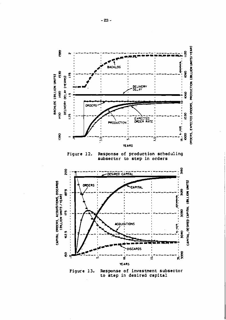
changes in desired capacity without overshoot o r instability. Similarly, the pro- duction scheduling decision can accommodate unanticipated changes in demand smoothly and without disruption. The next test examines the ability of the entire sector to respond to a change in demand. In the test, the sector faces a five per- cent unanticipated increase in orders at the start of year one. The delivery delay for capital is assumed constant.

The result (Figure 14) is a highly damped oscillation with a period of about twenty years. In contrast to the previous tests, production and capacity now overshoot orders, then undershoot slightly before reaching equilibrium. Because capacity (and production) lag behind orders, the backlog (and delivery delay) must rise. When production equals orders (in year six), backlog stops increasing and reaches its maximum. Delivery delay peaks slightly earlier. In order to reduce delivery delay to normal levels, production and capacity must continue to expand above orders. By year eight, delivery delay is once again normal, but production still rises due to growing capacity and industry reluctance to reduce utilization. By year ten, backlog has fallen enough to begin to force utilization down, but because firms prefer to maintain full utilization, output continues to exceed ord- ers , and delivery delay falls below normal as firms draw down their backlogs to preserve profitability. Faced with excess capacity, investment is cut back, and by the twelfth year, capacity begins to decline. For delivery delay to return to nor- mal, the backlog must rise, forcing output and capacity below orders. But when delivery delay has returned to normal, aapacity is once again insufficient, trigger- ing a second, though much smaller, overshoot.

The test shows that as the complexity of the system grows relative to the sim- plifying assumptions and decision rules used by the subsectors of the organization, the rationality of the organization's response to change is degraded. Y e t despite the overshoot, the system's response is, on the whole, still ra ther rational. The majority of the behavior is a direct oonsequence of the physical constraints facing the firms in the sector. Since production must lag behind orders backlogs mus t initially rise. Therefore output and aapacity mus t exceed orders to bring backlog back down. Overshoot is an inevitable consequence of the lags in expanding out- put. Oscillation, however, is not: the existence of oscillation is a consequence of decentralized decision making and the aggressiveness with which people attempt to correct perceived imbalances. Still, the system exhibits a high degree of damping (93% of the cycle is damped each period). And though output rises to a peak 65% greater than the'change in orders, rising delivery delays a r e arrested within four years, production settles within 2% of its equilibrium value after fifteen years, and utilization never drops below 97%. The behavior represents a good compromise between a speedy response and ~ tab i l i ty . '~

23~he 20-year cycle ie consistent with earlier modale of capital investment and empirical work on construction of Kuenete cycles. See Forrester (1982). Low (1980), and Mass (1975) for models of Kuznete-type cycles arising out of capital-investment policies. For empirical work on Kuenete cycles see, e.g., Hlckman (1963) and Kuenets (1930).

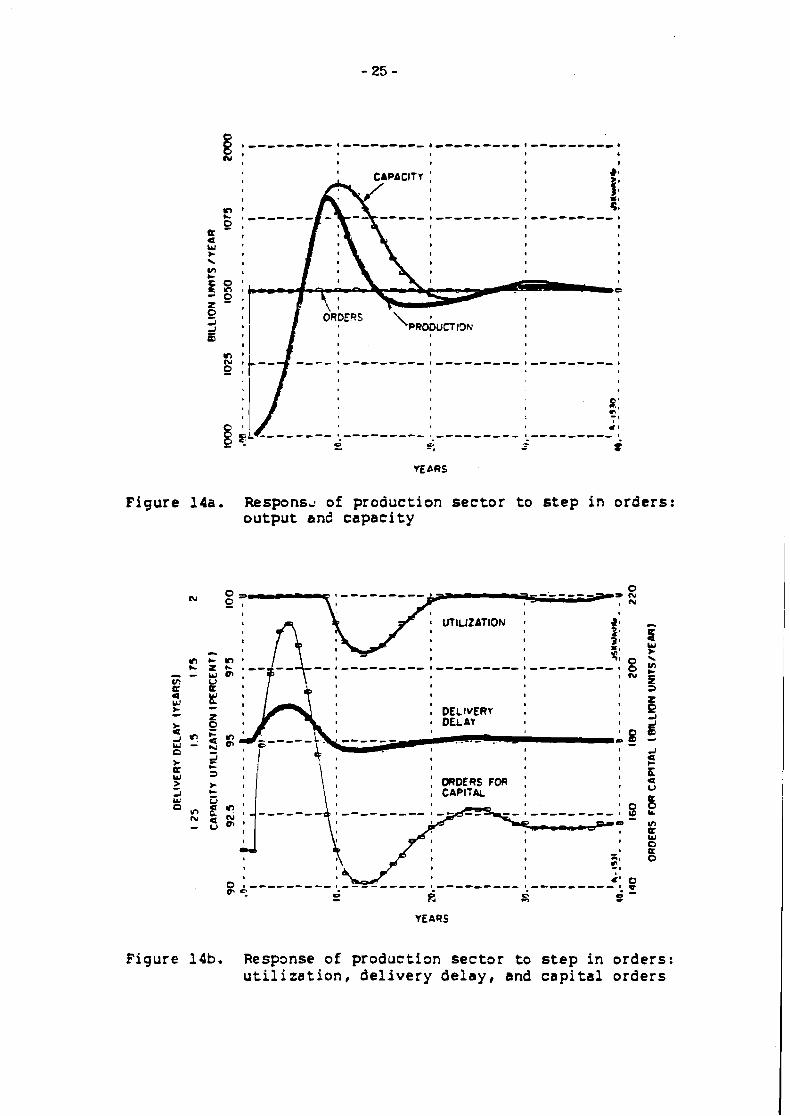
Figure 14a. R e s p o n s ~ of production s e c t o r t o s t e p i n orders: output and capaci ty

\ i I

: ORDERS FOR : CAPIT& I

YEARS

Figure 14b. Respmse of production s e c t o r t o s t e p i n orders: u t i l i z a t i o n , d e l i v e r y d e l a y , and c a p i t a l orders

TESTING THE DYNAMIC HYPOTEIESIS Having established the local rationality of the subsectors of the model, the

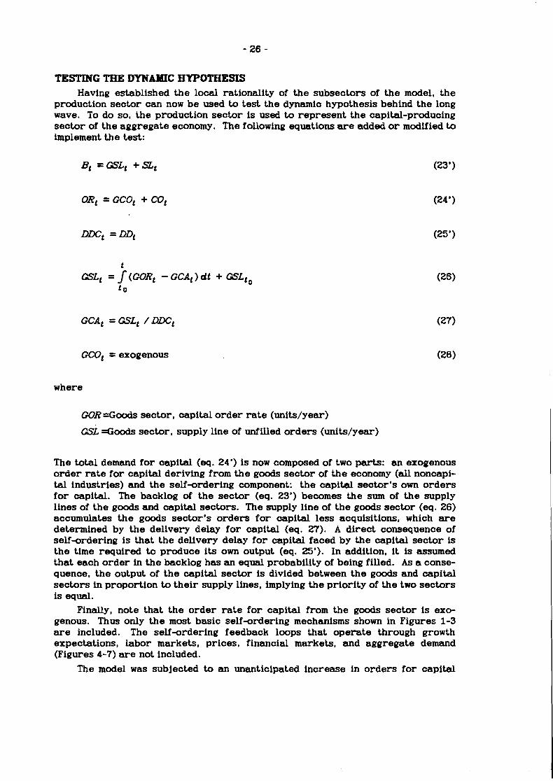
production sector can now be used to test the dynamic hypothesis behind the long wave. To do so, the production sector is used to represent the capital-producing sector of the aggregate economy. The following equations are added or modified to implement the test:

OR, = GCOt + Cot (24')

OCOt = exogenous

where

W R =Goods sector , capital order rate (units/year)

GSL =Goods sector , supply line of unfilled orders (units/year)

The total demand fo r oapital (eq. 24') is now composed of two parts: an exogenous o rde r rate fo r capital deriving from the goods sector of the economy (all noncapi- tal industries) and the self-ordering component: the capital seotor's own o rde r s fo r capital. The backlog of the sector (eq. 23') becomes the sum of the supply lines of the goods and capital sectors. The supply line of the goods sector (eq. 26) accumulates the goods sector's o rde r s f o r oapital less acquisitions, which are determined by the delivery delay f o r capital (eq. 27). A direct consequence of self-ordering is that the delivery delay f o r capital faced by the capital sector is the time required to produce i ts own output (eq. 25'). In addition, i t is assumed that each order in the backlog has an equal probability of being filled. A s a conse- quence, the output of the capital sector is divided between the goods and capital sectors in proportion to the i r supply lines, implying the priority of the t w o sectors is equal.

Finally, note that the order rate f o r capital from the goods sector is exo- genous. Thus only the most basic self-ordering mechanisms shown in Figures 1-3 are included. The self-ordering feedback loops that operate through growth expectations, labor markets, prices, financial markets, and aggregate demand (Figures 4-7) are not included.

The model w a s subjected to an unanticipated increase in orders for capital

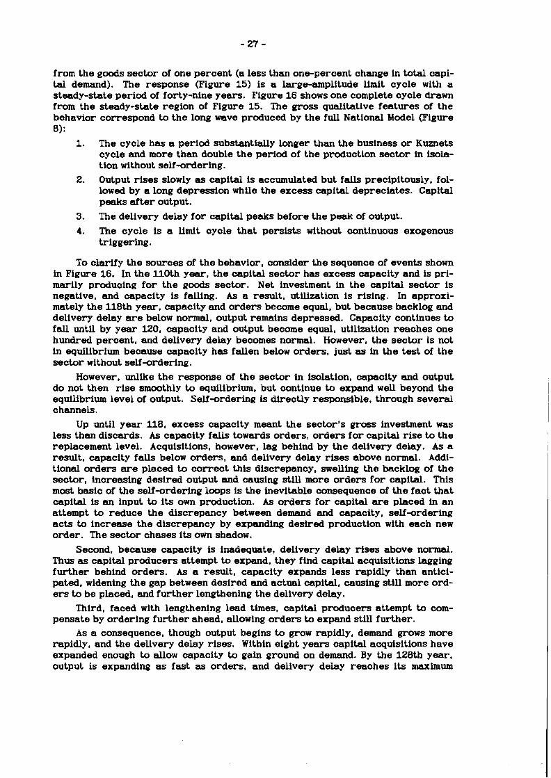
from the goods sector of one percent (a less than one-percent change in total capi- tal demand). The response (Figure 15) is a large-amplitude limit cycle with a steady-state period of forty-nine years. Figure 16 shows one complete cycle drawn f r o m the steady-state region of Figure 15. The gross qualitative features of the behavior correspond to the long wave produced by the full National Model (Figure 8) :

1. The cycle has a period substantially longer than the business or Kuznets cycle and more than double the period of the production sector in isola- tion without self-ordering.

2. Output rises slowly as capital is accumulated but falls precipitously, fol- lowed by a long depression while the excess capital depreciates. Capital peaks af ter output.

3. The delivery delay for capital peaks before the peak of output.

4. The cycle is a limit cycle that persists without continuous exogenous triggering.

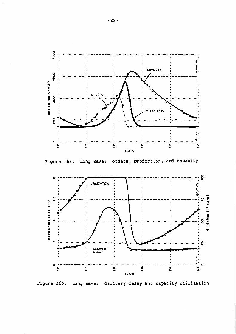
To clarify the sources of the behavior, consider the sequence of events shown in Figure 16. In the 110th year, the capital sector has excess capacity and is pri- marily producing for the goods sector. N e t investment in the capital sector is negative, and capacity is falling. As a result, utilization is rising. In approxi- mately the 118th year, capacity and orders become equal, but because backlog and delivery delay are below normal, output remains depressed. Capacity continues to fall until by year 120, capacity and output become equal, utilization reaches one hundred percent, and delivery delay becomes normal. However, the sector is not in equilibrium because capacity has fallen below orders, just as in the test of the sector without self -ordering.

However, unlike the response of the sector in isolation, capacity and output do not then rise smoothly to equilibrium, but continue to expand well beyond the equilibrium level of output. Self-ordering is directly responsible, through several channels.

Up until year 118, excess capacity meant the sector's gross investment w a s less than discards. As capacity falls towards orders, orders for capital rise to the replacement level. Acquisitions, however, lag behind by the delivery delay. As a result, capacity falls below orders, and delivery delay rises above normal. Addi- tional orders are placed to correct this discrepancy, swelling the backlog of the sector, increasing desired output and causing still more orders for oapital. This most basic of the self-ordering loops is the inevitable consequence of the fact that capital is an input to its own production. As orders for capital are placed in an attempt to reduce the discrepancy between demand and capacity, self-ordering acts to increase the discrepancy by expanding desired production with each new order. The sector chases its own shadow.

Second, because capacity is inadequate, delivery delay rises above normal. Thus a s capital producers attempt to expand, they find capital acquisitions lagging further behind orders. As a result, capacity expands less rapidly than antici- pated, widening the gap between desired and actual capital, causing still more ord- ers to be placed, and further lengthening the delivery delay.

Third, faced with lengthening lead times, capital producers attempt to com- pensate by ordering further ahead, allowing orders to expand still further.

A s a consequence, though output begins to grow rapidly, demand grows more rapidly, and the delivery delay rises. Within eight years capital acquisitions have expanded enough to allow capacity to gain ground on demand. By the 120th year, output is expanding as fast as orders, and delivery delay reaches its maximum

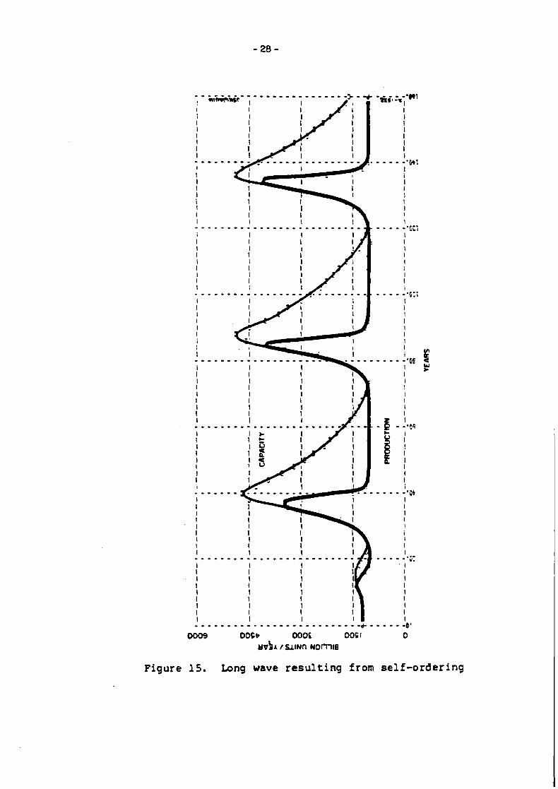
Figure 15. Long wave resulting f ram self-ordering

YEARS

Figure 16a. Long wave: o r d e r s , product ion , and c a p a c i t y

YEARS

Figure 16b. b n g wave: d e l i v e r y d e l a y and c a p a c i t y u t i l i z a t i o n

value. The sector's output now rapidly begins to catch up to orders, though ord- ers, through self-ordering, continue to rise even though they a r e now well above the equilibrium level. By the 132nd year, output overtakes orders and backlog reaches its peak. Delivery delay is now falling, reducing orders by accelerating acquisitions and reducing the required supply line. But though orders are now fal- ling, backlog and delivery delay remain wel l above normal, forcing capacity to expand further. By the 134th year, delivery delay and backlog have return to nor- mal, but capacity is much higher than its equilibrium level.

With output at record levels and orders plummeting, backlog and delivery delay reach and then drop below their normal values as firms attempt to maintain full utilization. The backlog is rapidly depleted, however, and utilization is forced down. Output drops precipitously, and the sector enters a period of depression with capacity f a r in excess of demand. Note that capacity continues to rise even after output has fallen. Though the sector's orders for capital peak in year 131 and then fall precipitously, capital already ordered continues to arrive, worsening overcapacity.24 And since the lead time for capital.drops below normal, capital on order is delivered faster than expected, expanding capacity beyond anticipated levels.

With its backlog depleted and capacity utilization a t 25%. the sector has, by year 139, cut gross investment to zero. Output and gross investment remain depressed for the next two decades as capacity slowly depreciates, until capacity once again equals orders and the cycle begins again.

COYMENTS ON THE BEAIJSH OF THE BEEIAVIOR The long cycle generated by the model with self-ordering closely resembles,

in qualitative terms, the long wave generated by the National Model. But the mag- nitude of the fluctuation is extreme: delivery delay expands to over 250% of nor- mal; capacity utilization falls to a minimum of under 25%; total gross investment falls by over 75% from the peak with investment in the capital sector collapsing to zero. In comparison, between 1929 and 1933, US real private investment fell 88%, real GNP fell by 30%, and unemployment reached 25%.

The extreme simplicity of the model is the cause of the extreme behavior. Since only the most basic channels for self-ordering are represented, the full bur- den of the disequilibrium pressures generated during the cycle must be borne by a few variables. One would expect that as additional structure and realism are added to the model, the burden borne by any individual channel would fall while the total amplification, to a first approximation, stayed the same. For example, the model excludes relative prices. In reality, as demand outstrips capacity, the price of capital would rise, easing some of the pressure on delivery delay by damping demand growth. A t the same time, higher capital prices would encourage expan- sion and reinforce self-ordering through the mechanisms outlined in Figure 6. Given the extreme simplicity of the model, extensive comparison of the magnitudes of the variables to historical experience is not warranted.

2 4 ~ recent example is provided by t h e commercial construction industry (Business Week, 4 October 1982, pp.94-98).

THE ROLE OF SELFrOBDERING The strength of self-ordering in equilibrium is governed primarily by the

capital/output ratio. As calculated in equation (4), the equilibrium multiplier effect created by self-ordering is given by I/ (I--COR/ ALC). Thus reducing the capital/output ratio should reduce both the amplitude and period of the cycle by reducing the magnitude of the capacity overshoot and hence the time required for oapacity to depreciate. Table 2 shows period, amplitude, and damping as a function of COR given the other parameters of the model. When COR a 0, self-ordering is eliminated, and the behavior approaches that of the sector in isolation with a period of twenty years and a damping ratio of 93%. As COR rises, damping falls dramatically while t h e period remains relatively constant. A t COR a l . 6 , damping is eliminated and the oscillation reaches a fixed steady-state amplitude. Further increases in COR rapidly lengthen the period and boost the amplitude. The results verify the crucial role of self-ordering in lengthening the natuml period of the accelerator mechanism portrayed in the production sector.

The other determinant of the strength of self-ordering is the average life of capital ALC. Altering ALC has two opposing effects. On the one hand, ALC controls the time required f o r excess capacity to depreciate during the depression phase, so shortening ALC should reduce the period. But shortening ALC also increases the strength of self-ordering, suggesting a larger amplitude. Table 3 shows that the amplitude is increased substantially as ALC falls. The period, however, is quite insensitive to ALC, and in fac t tends to shrink as ALC gets shor ter o r longer. Though a shor ter ALC implies fas ter decay of excess capacity, more rapid depre- ciation makes it more difficult f o r the capital sector to catch up to orders during the expansion phase. Output overtakes demand at a later and higher level, so even though excess capacity is eliminated more rapidly, more excess capacity is gen- erated, resulting in a reduction in period of only six years when ALC is reduced from twenty to ten years. Similarly, a longer ALC extends the time required to eliminate excess capacity but reduces the strength of self-ordering so that output overtakes orders at a much lower level. The results, particularly the decrease in period with longer ALC, show the period of the cycle to be determined primarily by the strength of the self-ordering loop and not the life of capital. The insensitivity to ALC shows the cycle is not created by the echo effect that figures in some explanations of the long wave.25

Self-ordering also operates through other channels. During the upswing of the cycle, rising delivery delays slow capital acquisition, fur ther augmenting the backlog and lengthening lead times. To test the importance of this channel, i t was assumed tha t the capital sector has absolute priority over the goods sector when demand fo r capital exceeds capacity, and is always able to receive capital within the normal delivery delay:

CA, = S L , / m

GCA, = PR, - CA, (26')

The result is a 37-year cycle with an amplitude 70% as large as the base case. The qualitative features are largely unchanged. With priority over o ther sectors, the

2 5 ~ o t h Kondrat iev and De W o w invoked t h e e c h o effect t o explain t h e period o f t h e long w a v e (Van Duiln 1983, pp.62; 67).

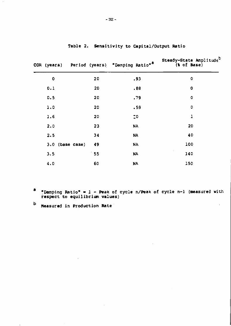
Table 2. S e n s i t i v i t y t o Capital/Output Ratio

Steady-State Ampl i rudeS COR (years ) Period (years ) .Damping ~ a t i o . ' ( 8 of Base)

0

0 . 1

0 .5

1 . 0

1 . 6

2 .0

2 .5

3 .0 (base case )

a 'Damping Ratiog = 1 - Peak of c y c l e n/Peak o f c y c l e n-1 (measured w i t h r e spec t t o equilibrium va lues )

Masured i n Production Rate '

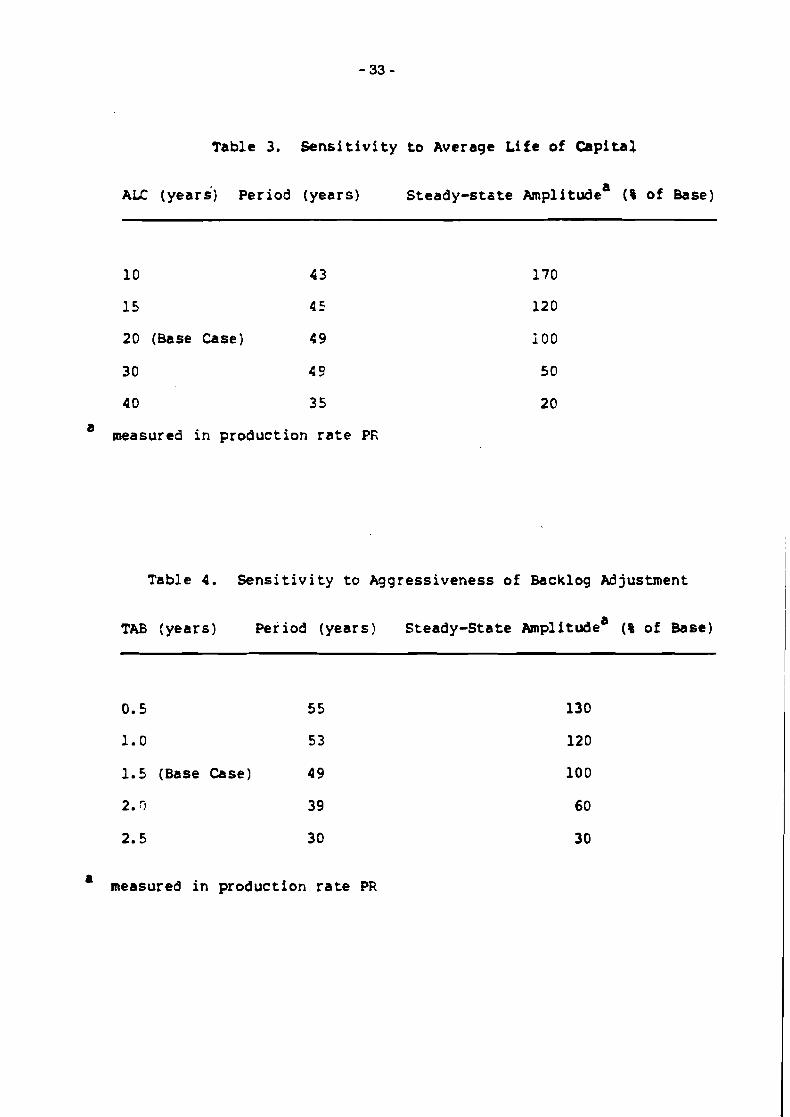
Table 3. S e n s i t i v i t y t o Average Life of Capital

AIL (years ) Period (years) Steady-state Amplitudea (8 of Base)

10 43

15 45

20 (Base Case) 49

30 4 9

40 35

a measured i n production r a t e PR

Table 4. Sens i t i v i t y t o Aggressiveness of Backlog Adjustment

TAB {years) Period (years) Steady-State &nplitudea ( 8 of Base)

0.5 55

1.0 53

1.5 (Base Case) 49

2.7 39

2.5 30

a measured i n production r a t e PR

capital sector can catch up to orders sooner and at a lower level. However, it is unlikely that such allocation exists. All firms, to some extent, are involved in pur- chasing from each other. Capital producers do not know the extent to which their customers are coupled through self-ordering and certainly do not consult an input/output table to assign priorities on the basis of the technical coefficients of their customers. The assumption of equal priorities is probably roughly correct in the aggregate, at last f o r an approximately competitive economy.26

Self-ordering also operates through the backlog correction (Figure 2). The aggressiveness. with which firms seek to maintain delivery delays at normal levels is controlled by the time to adjust backlog TAB. A s shown in Table 4, the period and amplitude are inversely related to TAB. While the amplitude is quite sensitive to TAB, the period is relatively less sensitive.

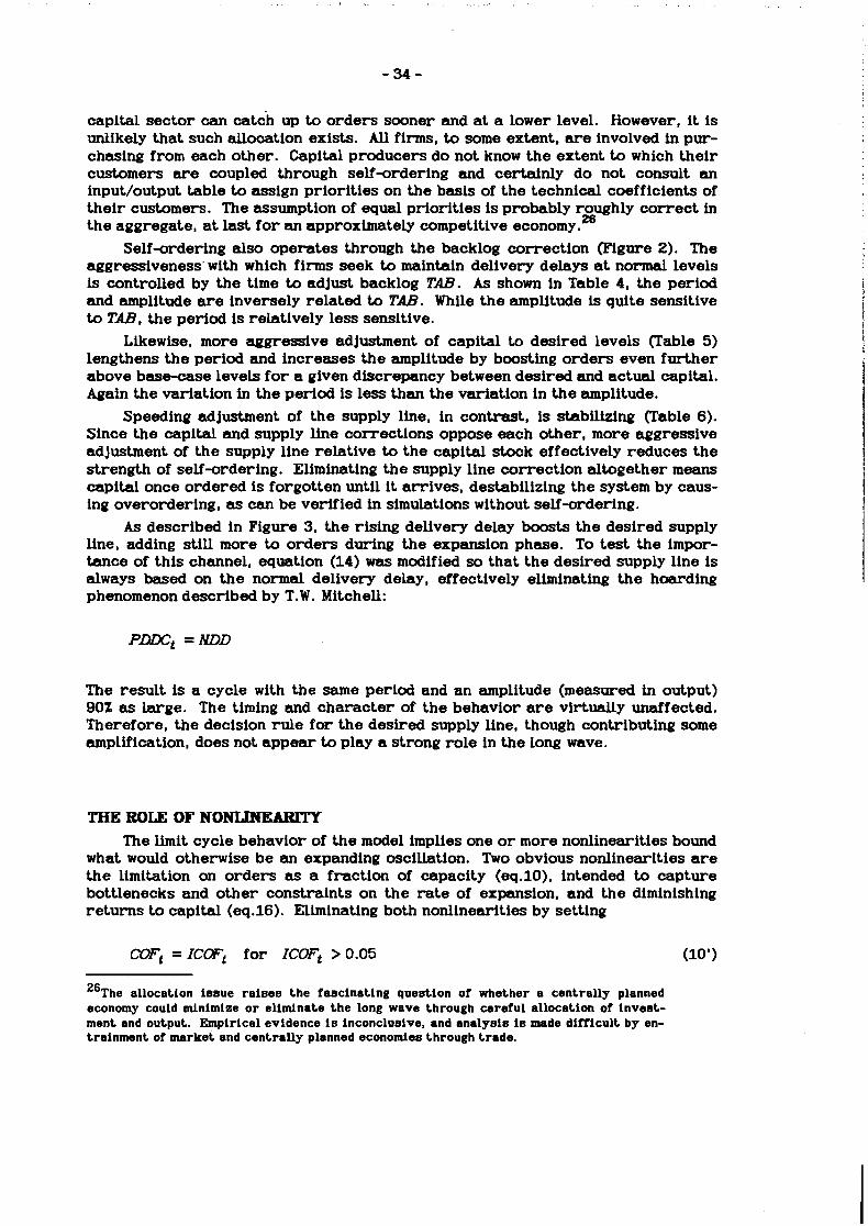
Likewise, more aggressive adjustment of capital to desired levels (Table 5) lengthens the period and increases the amplitude by boosting orders even fur ther above base-case levels f o r a given discrepancy between desired and actual capital. Again the variation in the period is less than the variation in the amplitude.

Speeding adjustment of the supply line, in contrast, is shbilizing (Table 6). Since the capital and supply line corrections oppose each other, more aggressive adjustment of the supply line relative to the capital stock effectively reduces the strength of self-ordering. Eliminating the supply line correction altogether means capital once ordered i s forgotten until i t arrives, destabilizing the system by caus- ing overordering, as can be verified in simulations without self-ordering.

A s described in Figure 3, the rising delivery delay boosts the desired supply line, adding still more to orders during the expansion phase. To test the impor- tance of this channel, equation (14) was modified so that the desired supply line is always based on the normal delivery delay, effectively eliminating the hoarding phenomenon described by T. W. Mitchell:

The result is a cycle with the same period and an amplitude (measured in output) 90% as large. The timing and charac ter of the behavior are virtually unaffected. Therefore, the decision rule for the desired supply line, though contributing some amplification, does not appear to play a strong role in the long wave.

THE BOLE OF NONLINEARITY The limit cycle behavior of the model implies one or more nonlinearities bound

what would otherwise be an expanding oscillation. Two obvious nonlinearities are the limitation on orders as a fraction of capacity (eq.10). intended to capture bottlenecks and other constraints on the rate of expansion, and the diminishing returns to capital (eq.16). Eliminating both nonlinearities by setting

2 6 ~ h e allocation ieeue r a i s e s t h e faecinating que&ion of whether a centrally planned economy could minimize o r eliminate t h e long wave through careful allocation of inveet- ment and output. Empirical evidence is inconclueive, and analyeis is made diff icult by en- trainment of market and central ly planned economies through trade.

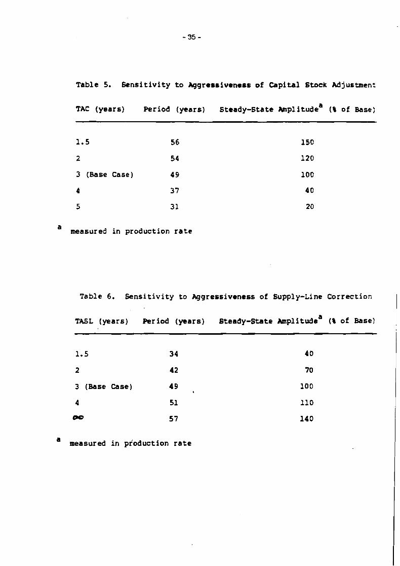
Table 5. Sens i t iv i ty t o Aggressiveness of Capital Stock Adjustment

TAC (years) Pcriod (years) Steady-State Ampl itudea (% of Base)

1 . 5 5 6

2 54

3 (Base Case) 49

4 37

5 31

a measured in production rate

Table 6 . Sens i t iv i ty to Aggressiveness of Supply-Line Correc t io~

TASL (years) Period (years) Steady-State Amplitudea (% of Base:

1.5 34

2 4 2

3 (Base Case) 49 *

4 51

00 57

a measured in production rate

yields a period of 75 years and an amplitude nearly 3.5 times greater than the base case." The test clearly shows constraints on ei ther the level or rate of capital expansion to be important factors in bounding the period and amplitude of the cycle. However, without these nonlinearities the cycle still reaches a finite steady-state amplitude, suggesting another nonlinearity is primarily responsible f o r bounding the oscillation. That nonlinearity is the capacity utilization formula- tion (eq. 2).

In both Figures 14 and 16, output falls below capacity when the backlog drops below a level consistent with the normal delivery delay, restraining the overshoot of output and preventing the backlog from.declining too f a r below its equilibrium value. If output w e r e always equal to capacity, however, backlog would decline further below its equilibrium value, forcing larger cutbacks in investment and des- tabilizing the cycle. Setting

without self-ordering leaves the period Largely unaffected but reduces the damping rat io from 93% to 35%. When self-ordering is added, equation (1") results in an expanding oscillation which soon drives backlog, delivery delay, and capital acquisitions below zero. A s fur ther confirmation of the importance of capacity utilization, the full model w a s simulated with

implying perfectly flexible capacity. The result is a highly damped response with a single overshoot of capacity above its equilibrium value.

Thus the crucial nonlinearity is the relationship between backlog and capa- city. While aonstraints on the rate or level of capacity expansion may limit the period and amplitude of the cycle, fundamentally it is the fact that output can only rise as aapacity grows that creates the disequilibrium, and the fact that output must fall as the backlog is depleted that l imits it.''

27glirninating only one of t h e nonlineari t ies simply allows t h e sys t em t o g rawfu r the r unti l t h e remaining cons t ra in t becomes binding.

"~hough t h e behavfor of t h e model is d d n a t e d by nonlinearity, ana lys is of t h e eigen- values of t h e l inearised sys t em verif ied t h e cruc ia l ro le of capacity ut i l isat ion in con- trol l ing damping. Linearizing around t h e in i t ia l equilibrium with eq.(lnn) (CV=l)a yie lds dominant eigenvalues correrrponding t o expanding oscillation wlth a period of 25.5 y e a r s and a growth r a t e of t h e envelope of i?IIX/year. In cont ras t , l inearizat ion with eq. (in") (CU=IP/E) yielded eigenvalues corresponding t o a highly damped oscillation with a period of 23.8 y e a r s and a decay r a t e of t h e envelope of lB%/year. Intui t ively, t he slope of CU determines t h e r e l a t i ve s t r eng ths of t h e osci l latory capital acquisition loop and t h e s tab le f i r s t -order production scheduling loop. During t h e expanrrion phase, ut i l ieat ion is a t its maximum, and t h e unstable loop dominates. As exces s capaci ty develops, CV fal ls , and dominance s h i f t s t o t h e s tab le loop, limiting t h e amplitude of t h e cycle.

The model presented here is not merely a set of equations which produce a long cycle. The decision rules portrayed in the model are consistent with the information-processing and decision making capabilities of economic agents. Further, the individual decision rules are locally or intendedly rational: they yield rapid. orderly, and appropriate adjustments to unanticipated shocks within the local environment of the organizational subunits responsible fo r the decision. Y e t as the complexity of the environment grows, the overall rationality of the system's response is degraded. The results demonstrate what Simon (1947, p.81) calls

"segments" of rationality.. . (the) behavior shows rational organization within each segment, but the segments themselves have no very strong interconnections.

The positive feedback loops created by self-ordering increase the amplitude and lengthen the period of oscillations created by the production and investment policies of the sector. policies which, from the vantage point of the firm, a r e quite rational. Indeed, an individual firm cannot distinguish orders that are par t of the "true" long-run demand from the "false" orders generated by amplification and self-ordering. A firm or management team that attempted to turn away orders or expand less aggressively on the grounds that it would cause overexpansion in twenty years would not Last long in the face of high delivery delays and rapid growth.

The results show that the dynamic hypothesis of self-ordering is sufficient to cause a long wave. given only the local rationality of the decision rules and the physical structure of capital accumulation. More precisely, the results show that self-ordering amplifies the disequilibrium pressures created by the interaction of locally rational decision rules and the Lags in capital acquisition within a firm, ver- ifying Forrester's statement (1977, p.534) that self-ordering "creates the 50-year cycle out of what would otherwise be a 20-year medium cycle in aapital acquisi- tion. "

The model shows only the most fundamental feedback loops created by self- ordering, relationships which primarily involve the physical determination and allocation of output, are necessary to generate a robust long wave. But the suffi- ciency of the basic self-ordering channels does not mean other mechanisms are unimportant o r irrelevant. Self-ordering also creates additional feedback chan- nels through, f o r example. Labor markets, growth expectations, prices, financial markets, and aggregate demand. These are portrayed in the full National Model. One would expect that adding these additional mechanisms would add to the net amplification created by self-ordering. strengthening the long wave while adding "fine structure" to the behavior and permitting realistic policy analysis.

The results should not be interpreted as excluding other mechanisms as arnpli- fying o r contributory factors in the long wave. However, those who would argue fo r the primacy of other mechanisms have yet to demonstrate the sufficiency of those mechanisms in a framework that permits reproducible testing. In particular. the model shows the long wave can arise with technology held completely constant (without even the technological changes implicit in varying the mix of capital and labor). The results suggest that the historical long-wave pattern in innovations is the result of entrainment by the physical process of self-ordering ra the r than vice-versa, as explained by Forrester (1977). and by Graham and Senge (1980). If the 'long-wave theory of innovation" more nearly describes the situation than the "innovation theory of the long wave" favored by the neo-Schurnpeterian school, policies directed at stimulating innovation may be insufficient to mitigate the

effects of the current long-wave downturn.29 These issues have important policy implications, and i t is hoped that the methodological framework illustrated with the single model presented here can provide the common ground f o r systematic exploration of the forces behind the long wave, contributing toward an integrated theory of disequilibrium economic behavior.

" ~ 0 t h Freeman ct a1. (1982) and Van Duifn (1983) argue for stimulus of innovation as prime components of an effective strategy to counter the long wave. While renewed com- mitment to R&D i s needed, these results suggest dealing with excess physical capacity may be more important (Mass and Senge 1981; Sterman 1983).

BEF'EBENCES Coen, R. (1975) "Investment Behavior, The Measurement of Depreciation, and Tax

Policy", American Economic Review. 65, 59-74.

Cyert, R., and J. March (1963) A Behavioral meory of the F E n n (Englewood Cliffs: Prentice-Hall).

Delbeke, J. (1981) "Recent Long-Wave Theories: A Critical Survey", fitures, 13, 246-57.

Dutton, J., and W. Starbuck (1971) Cbmputer Simulation QZ Human Behavior (New York: Wiley).

Forrester, J. (1976) "Business Structure, Economic Cycles, and National Policy", fitures, 8, 195-214.

Forrester , J. (1977) "Growth Cycles ", W Economist, 125(4), 525-43.

Forrester , J. (1979) "An Alternative Approach to Economic Policy: Macrobehavior from Microstructure" in Economic Issues of the Eighties, N. Kamrany and R. Day (eds.) (Baltimore: Johns Hopkins University Press).

Forrester , N. (1982) A Dynamic *thesis of Basic Macroeconomic Theory: Implications for Stabilization Policy Analysis, Ph .D . Dissertation, MIT.

Freeman, C. (1979) 'The Kondratiev Long Waves, Technical Change, and Unemploy- ment", in Structural Determinants of Employment and Unemployment, Vo1.2 (Paris: OECD), 181-96.

Freeman, C., J. Clark, and L. Soete (1982) Unemployment and Technical Innova- tion: A Study of Long Waves and Economic Davelopment (Westport, Conn. : Greenwood Press).

Goffman, E. (1959) m e Presentation @Self in Everyday Lve (Garden City, NY: Doubleday).

Graham, A., and P. Senge (1980) "A Long-Wave Hypothesis of Innovation", Rchno- logical Fbrecasting and Social Change. 17, 283-311.

Hickman, B. (1963) 'Tostwar Growth in the United States in Light of the Long-Swing Hypothesis", American Economic Review: Papers and Proceedings, 53, 490- 507.

Hogarth, R. (1980) Judgment and Choice (New York: Wiley).

Jorgenson, D. (1963) "Capital Theory and Investment Behavior", American Economic Review, 53, 247-59.

Jorgenson, D., J. Hunter, and M. Nadiri (1970) "A Comparison of Alternative Econometric Models of Quarterly Investment Behavior", Econornetrica, 38, 187-212.

Kahneman, D., P. Slovic, and A. Tversky (1982) Judgement Under Uncertainty: fihristics and Biases (Cambridge: Cambridge University Press).

Kleinknecht, A. (1981) "Observations on the Schurnpeterian Swarming of Innova- tions", fitures, 13, 246-57.

Kondratiev, N. (1935) "The Long Waves in Economic Life", Review of Economic Statistics, 17, 105-15.

Kuznets, S. (1930) Secular Movements in Production and Prices (New York: Houghton Mifflin).

Low, G . (1980) 'The Multiplier-Acceleratnr Model of Business Cycles Interpreted from a System Dynamics Perspective", in Elements of the System Dyhamics Method, J. Randers (ed.) (Cambridge: MIT Press), 76-94.

Mandel, E. (1980) Long Waves QZ Capitalist Development (Cambridge: Cambridge

University Press).

Mandel, E. (1981) 'Zxpldning Long Waves of Capitalist Development", FLtures, 13, 332-38.

March, J. (1978) "Bounded Rationality, Ambiguity, and the Engineering of Choice". WBU Journal ofEconomics, 9, 587-608.

Mass, N. (1975) Economic Cycles: An Analysis of Lhrderlying Causes, (Cam- bridge: MIT Press).

Mass, N. (1980) 'Stock and Flow Variables and the Dynamics of Supply and Demand", in Elements @ t h e System Dgmamics Method, J . Randers (ed.) (Cam- bridge: MIT Press), 95-114.

Mass, N. and P. Senge (1981) "Reindustrialization: Aiming for the Right Targets", Technology Review, Aug ./Sept., 56-65.

Mayer, T. (1960) ''Plant and Equipment Lead Times", JoumaZ ofacLsinass, 33,127- 32.

Mensch, G . (1979) Stalemate in Technology, (Cambridge: Ballinger).

Mensch, G., C. Coutinho, and K. Kaasch (1981) "Changing Capital Values and the Propensity to Innovate", Futures, 13, 276-92.

Merton, R. (1936) 'The Unanticipated Consequences of Purposive Social Action", Sociological Review, 16, 894-904.

Metzler, L. (1941) 'The Nature and Stability of Inventory Cycles", &view of Economic Statistics, 23, 113-29.

Mitchell, T. (1923) 'Competitive Illusion as a Cause of Business Cycles", m a r t e r l y Jounzal of Economics, 38, 631-52.

Mitchell, W. (1941) Business Cycles and Thetr Causes (Berkeley: University of California Press, Reprint Series edition, 1971).

Morecroft, J. (1983) 'System Dynamics: Portraying Bounded htionality", Omega, 11, 131-42.

Namenwirth, Z. (1973) 'The Wheels of Time and the Interdependence of Value Change", Journal @ Interdisciplinary &tory, 111, 649-83.

Neff , T. (1982) 'Short-Term Vulnerabilities: The World Oil Market in Transition", Working Paper MIT-EL82-OOlWP, Energy Laboratory, MIT, Cambridge, MA 02139.

Nelson, R. and S. Winter (1982) An Evolutionary Theory of Economic Change (Cambridge: Belknap Press of Harvard University Press).

Randers. J. (1980) 'Guidelines f o r Model Conceptualization", in ELtments of the *stem Dynamics Method, J . Randers (ed.) (Cambridge: MIT Press), 117-139.

Rostow, W. (1975) 'Xondratiev, Schumpeter and Kuznets: Trend Periods Revisited" Journal ofEcommtic History, 35, 719-53.

Rostow, W. (1978) The World Economy: History a d Prospect (Austin: University of Texas Press).

Schumpeter, J. (1939) Business Cycles (New York: McGraw-Hill)

Senge, P. (1978) The *stem Dynamics National Model Investment F'unction: A Comparison to the Neoclassical Investment FLnction. Ph.D. Dissertation, MIT.

Senge, P. (1980) "A System Dynamics Approach to Investment Function Formulation and Testing", Socio-Economic Running Sciences, 14, 269-80.

Senge, P. (1982) 'The Economic Long Wave: A Survey of Evidence", Working Paper D-3262-1, System Dynamics Group, MIT, Cambridge, MA 02139.

Simon, H. (1947) Administrative Behavior (1st ed.; New York: MacMih) . Simon, H. (1957) Models of Man (New York: Wiley).

Simon, H. (1978) "On How to Decide What to Do", WBU Jounrcrl of Economics, 9, 494-507.

Simon, H. (1979) "Rational Decision Making in Business Organizations", Amertcan Economic Reubw, 69, 493-513.

Sterman, J. (1980) 'The Use of Aggregate Production Functions in Disequilibrium Models of Energy-Economy Interactions", Working Paper D-3234, System Dynamics Group, MIT, Cambridge, MA 02139.

Sterman, J. (1981) m e Enetgy Ykahsition and f ie Economy: A System Qmamics Approach (2 vols.), Ph.D. Dissertation, KIT.

Sterman, J. (1982) 'Zconomic Vulnerability and the Energy Transition", Ehergy %stems and Policy (Forthcoming), Working Paper D-3356-1, System Dynamics Group, ME, Cambridge, MA 02139.

Sterman, J. (1983) 'The Long Wave" (letter), Science, 219 (18 March), 1276.

Tinbergen, J. (1981) 'Xondratiev Cycles and So-Called Long Waves: The Early Research", f i tures , 13, 258-63.

Tversky, A., and D. Kahneman (1974) "Judgement Under Uncertainty: Heuristics and Biases", Science, 185, 1124-31.

Van Duijn, J. (1977) 'The Long Wave in Economic Life", Lk Economist, 125, 544-76.

Van Duijn, J. (1981) ''Fluctuations in Innovation Over Time", Fbtures, 13, 264-75. Van Dui jn, J. (1983) The Long Wave in Economic Lve. (London: Allen and Unwin). Weber, R. (1980) "Society and Economy in the Western World System", SociaZ

Fbrces, 59(4), 1130-48.

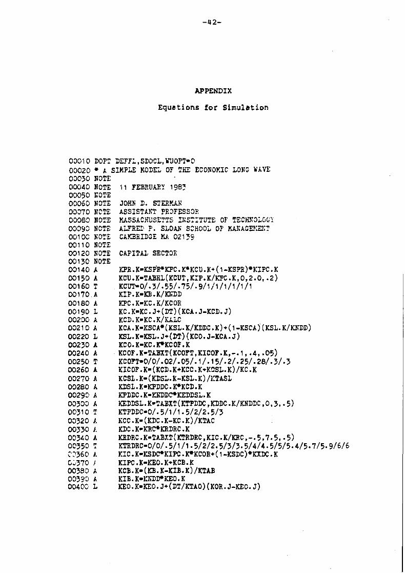
APPENDIX

Equations for Simulation

03310 DOPT DEFFL,SDOCL,hVOPT10 03020 h SIMPLE NODEL OF THE ECONOKIC LONG WAVE 09330 RITE 00040 NOTE 1 1 FEBSUUY 1983 00050 KOTE 00060 N3TZ JOHK 3. STD.KAK 03270 NCTE ASSISTLFT PR3FESS33 00965 HOTS YASSXCHL'SETTS IISSYITUTE OF TECKh'3LSGT 03393 NCTE A-RE9 ?. SLOAX SCHOOL OF YLAh'AGP:ZI;T 001 02 KOTE CXFBBIDSE Yd. 021 >3 03110 NOTE 09120 KaTE CAPITAL SECTDE OGl3C NOTE 03140 k DR. K-KSP'PKPC. K ~ K C U . K+ ( 1 -KSPR)*KIPC . K 03150 A KCU.K-TABHL(KCUT,KIP.K/L?C.K,O,~.~, .2) 00160 T KCWO/*3/*55/*75/*9/1/1/1/1/1/1 00170 A KIP. K-KB. K/SUiDD 001 80 b KPC.K-KC.K/Y.COfi 00190 L KC. K-KC. J+(DT) (KCA. J-KCD. J) 00200 A KCD. K-KC . K/ULC 00211) k KCA. K-XSCA*(KSL. K/KDDC. K) + ( 1 -KSCA) (KSL. K/KNDD) 00220 L KSL. K-KSL. J+ (DT) (KCO. J-KCA . J) 00230 A KCO. K-KC .RKCOF. K 00240 A KCOF. K-TABXT(KCOPT,KICOF.K,-. 1, .4, .05) 00250 T KCOFT-0/0/.02/.05/.1/.15/.2/.25/.28/.3/.3 00260 A KICOF. K- (KCD.K+KCC. K+K~SL.K) /KC. K 03270 1. KCSL. K- (KDSL. K-KSL.K) /I:TASL 09280 X KDSL.K-KPDDC.PKCD.K 00293 h l3'DDC.K-l3DDPKEDDSL.K 09333 Ir KEDDSL. K-TUX?? ( KTPDDC , KDDC . K/KNDDC , 0 ,3, .5) 0031 0 ? KTPDDC-O/. 5/1 /I .5/2/2.5/3 03320 A KCC .K- (KDC .K-KC .K) IKTAC 00330 1. KDC . K-ACRC*KRDRC. K 03343 A KBDRC . K-TABxT(KTRDRC, KIC . K/KRC, - .5,7.5, -5) 00350 T KTRDRC-O/O/- 5/1/1 5/2/2.5/3/3.5/4/4.5/5/5-4/5.7/5- 9/6/6 3 3 6 0 A KIC . K-YSDPKIPC PKCOR+ ( 1 -KSDC) *KXDC. K 62370 1 K1PC.K-KEO.K+KCB.K 00380 A KCB.K-(D. K-K1B.K) /KTAB 00393 h KIB . K-lCXDVKEO. K 0040~ L mo.~-mo. J+(DT/KTAO) (KOR. J-KEC. J)

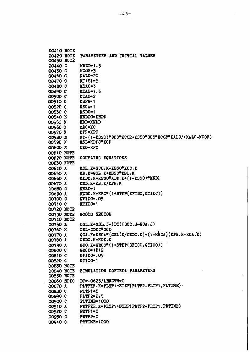
0041 0 NOTE 00420 NOTE PARAMETERS AND INITIAL VALUES 00430 NGTE 00440 C 1a~~>1.5 00450 c KCOR-3 00460 C KALC-20 OW70 C KTASb3 00480 C KTAC-3 00490 c KTAB- 1 5 00500 C KTAOI 2 00510 C KSPR- 1 00520 C KSCA- 1 00530 c KSDC-1 00540 h' ICNDDC- D D D 00550 8 KDD-KBTDD 00560 N KRC-KC 00570 N KPR-KPC 00580 N KC- ( 1 -KSSO)*GCPKCOR+KSSWGCO,KCOETKALC/ (KALC-KCOR) 00590 h' K S I r K D D P K C D 00600 h' KEOIKPC 0061 0 NOTE 00620 lOTE COUPLING EQUATIONS 00630 NOTE 00640 A KOB K-CCO. K+ICSSO,KCO. K 00650 A ICB. K-CSL. K+KSSD+KSL. K 00660 A KDDC. K-KSSWKDD. K+ ( 1 -KSSO)*KKDD 00670 A KDD.K-KB.K/KPR.K 33680 C KSSO-1 00690 A mC. K-KRP ( 1 +STEp(KFIDC, KTIDC) ) 00700 C KPIDC- 05 00710 C KTIDCI 1 00720 NOTE 00730 NOTE GOODS SECTOR 00740 NOTE 00750 L CSL. K-CSL. J+ (DT) (KO. J-CCI. J ) 00760 rJ CSL-CDDPCCO 00770 A GCA. K-KSC~(GSL:K/CDDC. K) + (1 -&A) (DR. K-KCA.~) 00780 A GDDC K-KDD X 00790 A CCO.K-CRCV(I +S!!EP(CPICO, GTICO))

.00800 C CRCOllEl2 00810 C CFI Ce. 05 00820 C GTICO- 1 00830 NOTE 00340 NOTE SIMULATION CONTROL PARMETERS 03850 NOTE 00860 SPEC DT-.0625/LEISGTH*O 00870 A PLTPEB . K-PLTP1 +STEP(PLTP2-PLTP1, PLT~XE) 00880 C PLTPI -0 mego c ~ ~ ~ ~ 2 1 2 . 5 00gOO C PLT-1000 00910 A PRTPER . K-PRTPI +STEP(PRTPZ-PRTPI , PRTIXE) 00920 C PRTP1-0 00930 C PRTP2- 0 00940 C PRTI13E- 1 000

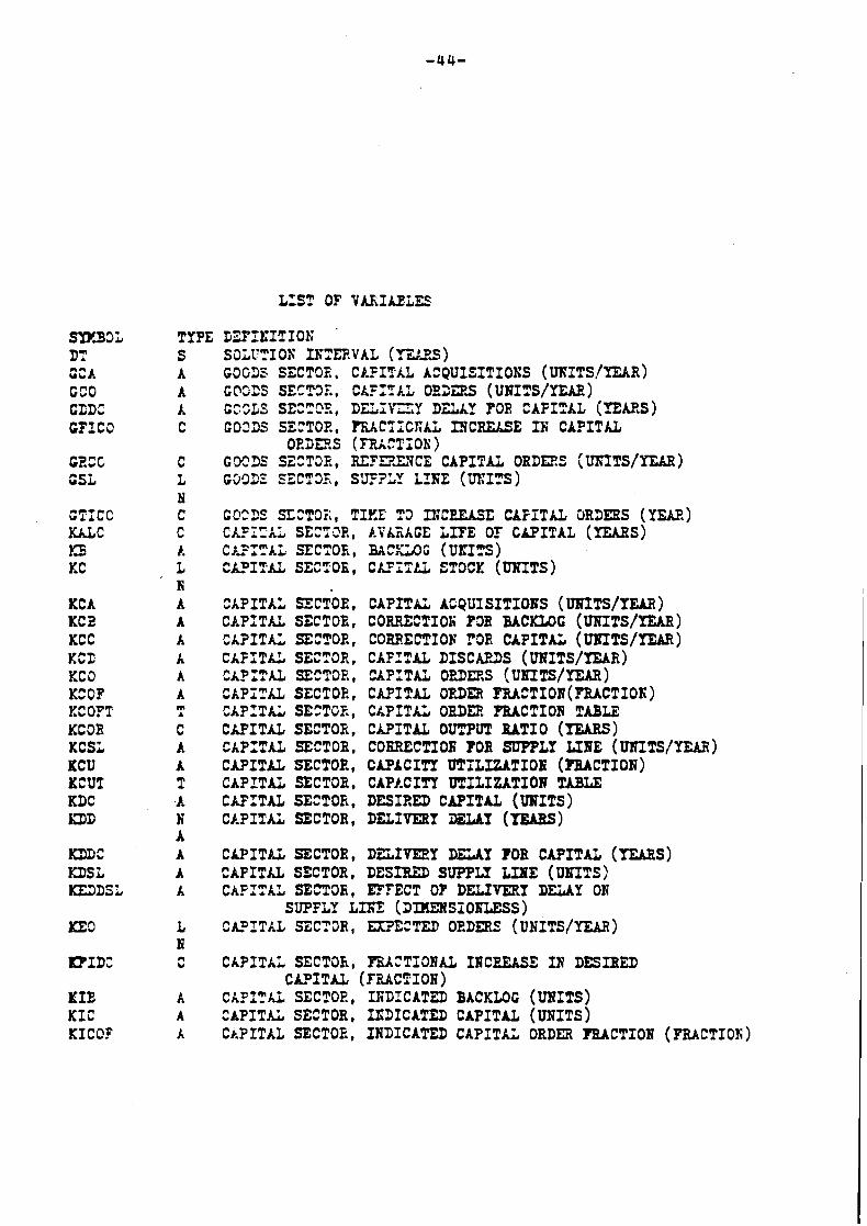
L I S T OF Y M i I U i E S

S V 3 9 L D": GCA CCO CZDt:

CECC

K C h KC E KCC KCC. KC O KC OP KC OPT KCOR KCSL KCU K C U l KDC KDD

KDDC KDSL KE3DSL

T Y P E D S P I E I T I O X S S O L P T I O S IICTERVAL (m.E~) A COG35 S E C T O E , C L F I T X L A C Q U I S I T I O X S ( ~ I T S I Y E ~ R ) A CQSCS S E C T 3 6 , C t F I l k L O E 3 D S (UNITS/YEIIE) h CSSLS SEZTC\F,, D L I I T Z Y DELAY FOR C A P I T A L ( T E E S ) C C O 3 3 S SECTOF!, R iXCIICXCIL E I C R E I S E I N C A P I T A L

O E 3 E . S ( F R A C T i O K ) C G X 3 S S X T 3 E , R E F D . L i C E C A P I T A L 0RDEP.S [ U E I T S / Y E A R ) L C 0 3 C Z S Z E T 3 3 , S V E ? L Y LIKE (UT:ITS) P C C0238 ! X Z T 3 B l T I X L T 3 IX:CEEASE CAPITAL OR3EKS (YEAR) C ChP2ZL SECTORl LFAEACE L I F E O F C h P I T A L (YEARS) I C ~ 3 I T A i S E C T O b , B A C X X C ( U G f Z S ) L CeITAL SECTOK, C h F I T I L S T 3 C X ( U H I T S ) I A CAPITAL SLCTOE, CAPITAL AGQUISITIOIS ( ~ T S / Y E A R ) A C P - P I T U S E C T O E , CORRECTIOIi P3R BACKLOC (UXITS/YEAR) k C A P I T A L SECTOR, COBF.ECTIOF !'OR C A P I T A L ( U f n T S / T E A R ) h C A F I T h L S E Z T O R , C A F I T A L D I S C A P J S (URITS/TEAR) A C A P I T A L SEC?DE, C A P I T A L O D E S ( U B I T S / Y E A R ) A C A P I T A L S E C T O R , C A P I T A L O R D m ~ C T I O R ( P B A C T I O N ) T C A P I T A L SEZTOFI, C A P I T A L ORDER FRACTION TABLE C C A F I T A L S E C T O E , C A P I T A L O t E P U T U T I O ( T E A R S ) A C A P I T A L SECTOR, COERECTIOI; FOB S U P P L Y X J B E (UIOITS/YEAR) A C A P I T A L S E C T O E , CAPACITY U T S L I W T I O H ( ~ B A c T I O B ) T C A P I T A L SECTDR, CAP)-CITY U T I L I W T I O f l TABLE A C A F I T A L SECTOR, D E S I R E D C A P I T A L (URITS) N C A P I T A L SECTOR, DELIVERY DZLAX (TEARS) A A C A P I T A L SECTOR, D Z L I m . Y D U T FOR C A P I T A L (TEABs) A C A F I T M , SECTOR, D E S I R Z D SUPPLY LIEE (UNITS) b C A P I T A L SECTDB, E F F E C T O F DELIVERY DELAY ON

SUPFLY L I K E ( X K E N S I O S L E S S ) L SAFITXL S C T D R , EXF'E2TEJI O R D m E (uNITS/YEAR) N Z C A P I T A L S E C T D h , P I U C T I O N A L I H C E E k S E IN D E S I R E D

C ~ I T L I L (TILACTIOH) X C A P 1 Tfi SECTOF!, IXDICATZD BACKLOG (UNITS) A C A P I T A L SECTOR, I C 3 I C A T E D C A P I T A L ( U N I T S ) b C A P I T A L SECTOE, I N D I C A T E D C A P I T A L O R D m ? E A C T I O R (PRACTIOX)

K I ? K I P C KNDD IQYDDC KOR KPC KPDDC KPR

KSPB KSSO KT.4B KTX C E X 6 KTASL KTIDC KTPDDC:

mc LENGTH P L T W P L T P E R P L T P 1 P L T P Z P R T M E P R T P mTP1 PRw2 STEP TABHL TABXT

C A P I T A L SECTOR, I N D I C A T E D PRODUCTIOB (UKITS/YEAR) C P P I T A L SECTOR, I K D I C A T E D PRODUCTION CAPACITY (UBITS/YEAR) C A P I T A L SECTOB, I J O I W L DELIVERY D E W Y ( m S ) C A P I T A L SECTOR, N O B l U L DELIVERY D E W Y FOR C A P I T A L (YEARS) C A P I T A L SECTOB, ORDEX RATE (UNITS/YEAR) C A P I T A L SECTOR, PRODUCTION CAPACITY (UEZ'S/YEAR) C A P I T A L SZCTCIS, PEXCEIYEI) DELIVERY DELAY POR C A P I T A L (YEARS) C A P I T A L SECTOB, PEODUCTIOB BATE ( U N I T S / T E A R )

C A P I T A L SECTOR, BEFEBEBCE C A P I T A L (UNITS) C A P I T A L SECTOB, U T I O OF D E S I R E D TO REFERENCE

C A P I T A L ( D I X E N S I O E L E S S ) C A P I T A L SECTOB, SWITCH POR C A P I T A L A C Q U I S I T I O N S

( D I ~ S I O I L E S S ) C A P I T A L SECTOB, S Y l T C H FOR D E S I R E D C A P I T A L (DIHENsIoHLESS) CAFITAL SECTOR, SUPPLY L I N E (UMTS)

C A P I T A L SECTOR, S U I T C E FOR PRODUCTION ( DIKENSIONLESS ) CAPITAL SECTOR, SUITCH FOR SELF OBDER~RG ( D ~ N S I O I L E S S ) C A P I T A L SECTOR, TIME TO ADJUST BACKLOG (YEARS) CAPITAL SECTOB, T I M E TO ADJUST C A P I T A L (YEARS) C A P I T A L SECTOB, T I M E TO AVERAGE ORDERS ( P E A R S ) C A P I T A L SECTOR, TIKE TO ADJUST SUPPLY L I N E (YEARS) C A P I T A L SECTOB, T I M E TO INCREASE D E S I R E D C A P I T A L (YEAR) C A P I T A L SECTOB, TABLE FOR P E R C E I V E D DELIYERY

DEL4Y FOB C A P I T A L C A P I T A L SECTOR, TABLE POR R A T I O O F D E S I R E D TO

B E P E B m C E C A P I T A L C A P I T A L SECTOB, EXOGENOUS D E S I R E D C A P I T A L ( U N I T S ) S l n U L A T I O E r s J G T H (TEABS) P L O T START TIHE (w) PLOT P E R I O D ( Y E W ) P L O T P E R I O D 1 (YEARS) PLOT P E R I O D 2 (YEARS) P R I N T START T I H E (TEAB) P R I N T P E R I O D (TEARS) P R I ~ PERIOD I (TEARS) P R I N T P E t I O D 2 (YEARS) S r n PURCTIOl'I FUNCTION POR HONLIHEAR B E L A T I O R S H I P FUNCTION FOR H O H L I l E A B B E L A T I O X S H I P