a simplified -a final copy

A Simplified Practical Procedure for Evaluation of System

Performance for A Line of Sight Relay

Dr. Jassim M. Abdul-Jabbar Computer Engineering Department, College of Engineering, Basrah University

:Abstract

The aim of this paper is to design and evaluate hop calculations and system performance for line of sight (LOS) radio relay links utilizing a simplified proposed procedure. Such a procedure is simulated for the determination of both hop calculations and system performance. The practical procedure of this paper has been ordered in a manner to solve up to 95% of the hop design problems encountered in practice. Two examples with different specifications and different required outage time are examined to fulfill the Committee Consultative International Radio (CCIR) recommendations. Key words: hop calculations, system performance, line of sight, radio relay links, outage time.

أسلوب عملي مبسط لحساب مواصفات الأداء لمنظومة اتصالات تعمل

البصر بموجات تنتشر بخط

جاسم محمد عبد الجبار. د جامعة البصرة, كلية الهندسة, قسم هندسة الحاسبات

:الخلاصة

ذا البحث هو ل بموجات إالغرض من ه ام يعم ل لموصفات الاداء لنظ صميم متكام اء ت عطرح صر تنتشر بخط الب ي مقت ل من . باستخدام اسلوب عمل رح لك ذا الاسلوب المقت اة ه م محاآ ت

.حسابات الفجوة ومواصفات الاداء للمنظومات المراد تصميمها عن طريق الحاسبةل عت لح ث وض ذا البح ي ه ة ف وات المقترح ر ٪95الخط ذت بنظ صميم أخ شاآل الت ن م م

ة ددات العملي ار المح و . الاعتب ذه الخط رت ه ي أختب ين ف ومتين مختلفت ى منظ ة عل ات المقترحل ن العم ة ع روج المنظوم ت خ ي وق فات وف ـ المواص ات ال ي متطلب ائج تلب د ان النت د وج وق

CCIR.

Iraq J. Electrical and Electronic Engineeringالمجلة العراقية للهندسة الكهربائية والالكترونية Vol.5 No.1 , 2009 2009 ، 1 ، العدد 5مجلد

12

1. Introduction

Reliability has two meanings in the microwave communication business; first there is the conventional meaning concerning the ability of the equipment to stay in service for extended periods with minimum attenuation. The other aspect of reliability is the transmission reliability which is a measure of system engineering, propagation characteristics, and the ability of equipment to yield high quality performance through adverse transmission conditions [1] - [3]. The aim of the hop calculations is to define transmitter's output power, feeder sizes and antenna diameters in order to achieve the required system performance. The transmission quality of a digital radio link is defined according to the percentage of time, in which a given Bit Error Rate (BER) is exceeded. The performance calculation may be divided into two parts of different nature. First, for a given set of parameters, the fading margin at the receiver input may be calculated. Second, on the basis of the resulted fading margin, a statistical calculation giving the transmission quality (and/or availability) is made. This paper is outlined as follows: Besides this introduction, different hop calculations are presented in section 2. Section 3 contains system performance for different fading phenomena. Space and frequency diversities are described in section 4 with their comparison being outlined in section 5. Section 6 contains the design procedure. Two design examples are treated in section 7. Finally, some conclusions are given in section 8.

2. Hop Calculations 2.1 Empirical obstruction loss The clearance of the hop may be allowed to be smaller than the value

given in reference [4], if it is very difficult or unduly expensive to obtain the sufficient clearance. Slightly obstructed paths lead in many cases to acceptable performance if the obstruction is caused by an isolated sharp-edged obstacle (e.g. mountain ridge, a nonexistent case in our path), where as smaller amounts of reduction in the clearance can be tolerated if the obstacle is sphere shaped (e.g. sea or flat terrain, an actual case in our path). The additional attenuation caused by the terrain (for earth curvature factor k=4/3) must be included in the performance calculations [4],[5]. In obstructed hops, one must always consider the possibility of deep fading of long duration owing to exceptionally small k-values. The clearance varies very rapidly with the value of k, in practical for long hops [4]. On obstructed hops, the diffraction loss (Lad) over average terrain can be approximated by

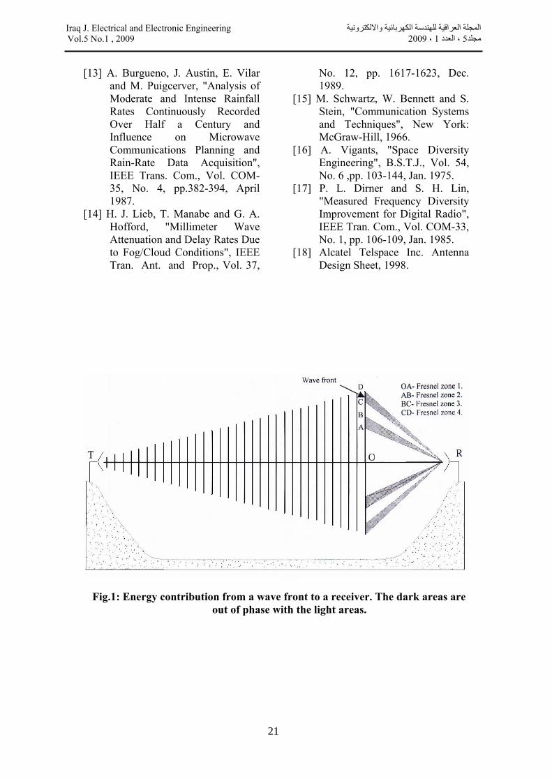
(1) where Lad is the additional (diffraction) attenuation (dB), F1 is the radius of the first Fresnel zone (m) and e is the clearance (m) (negative, if the obstacle extends above the line of sight). Range of validity: e/F1 is the range of (-2, …. +0.5 ). A simplified physical explanation of obstruction losses is shown in Figs. 1, 2 and 3. In Fig. 1 a succession of unobstructed radio wave fronts are shown progressing from the transmitter to the receiver. The whole surface of each individual wave front contributes energy to the receiving antenna. However, energy from some portions of the wave front tends to cancel energy from other portions because of differences in the total distances traveled. The shaded areas in Fig. 1 show the energy paths that cancel some


13

of the energy transmitted by the paths shown un-shaded. The cancellation is such that half of the energy reaching the receiver is canceled out. Most of the energy that is received is contributed by the large un-shaded central area of that portion of the wave front that is closest to the receiver. Fig. 2 gives an obstacle raised in front of the wave so that all of the wave front below the line of sight is obstructed. Fig. 3 shows that the obstruction is lowered, so that all of central zone is exposed; the power received by the receiving antenna is even greater than it would be if the obstacle was not there. The loss should be calculated for the minimum value of the normalized clearance e/F1, i.e. for the most prominent obstacle. The additional loss given by Eq. (1) is sketched in Fig. 4. Based on general scaling experience in path engineering, the empirical loss expression can be applied at frequencies from 2 to 11 GHz on most practical paths between 32 and 48km in length [5]. Investigations show that the additional losses are very sensitive to the antenna height and any small change in antenna height may cause large amount of additional losses. This may be easily observed from Fig. 5.

2.2 Antenna branching loss Antenna branching loss (Lbr) depends on the equipment configuration (in particular, the protection method used), the number of radio channels connected to antenna branching, and on the used frequency band. Attenuation varies greatly in different systems, so Lbr must be taken from the equipment data sheets [6], [7].

2.3 Feeder loss Feeder loss depends on the length and type of the feeder line, and on the ratio frequency. In loss calculations, losses of connecting cables and

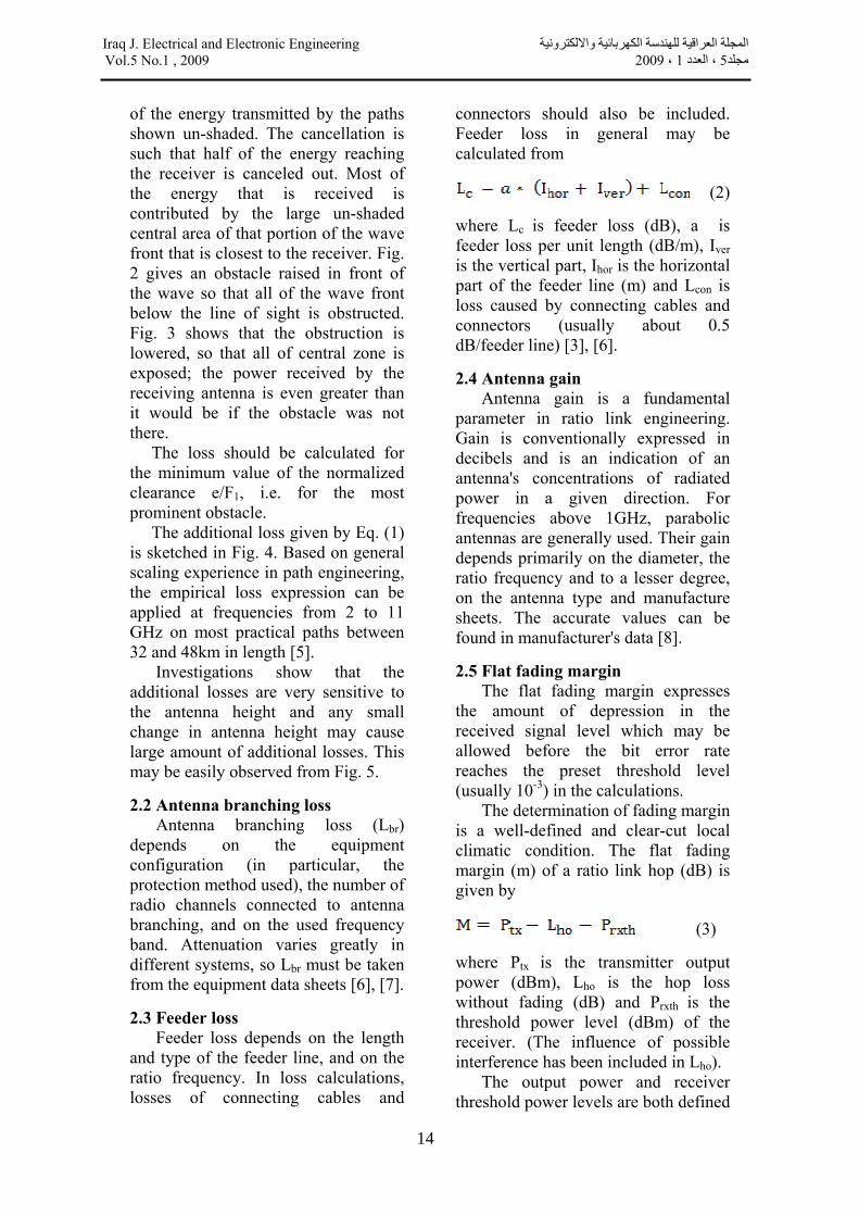
connectors should also be included. Feeder loss in general may be calculated from

(2) where Lc is feeder loss (dB), a is feeder loss per unit length (dB/m), Iver is the vertical part, Ihor is the horizontal part of the feeder line (m) and Lcon is loss caused by connecting cables and connectors (usually about 0.5 dB/feeder line) [3], [6]. 2.4 Antenna gain Antenna gain is a fundamental parameter in ratio link engineering. Gain is conventionally expressed in decibels and is an indication of an antenna's concentrations of radiated power in a given direction. For frequencies above 1GHz, parabolic antennas are generally used. Their gain depends primarily on the diameter, the ratio frequency and to a lesser degree, on the antenna type and manufacture sheets. The accurate values can be found in manufacturer's data [8]. 2.5 Flat fading margin The flat fading margin expresses the amount of depression in the received signal level which may be allowed before the bit error rate reaches the preset threshold level (usually 10-3) in the calculations. The determination of fading margin is a well-defined and clear-cut local climatic condition. The flat fading margin (m) of a ratio link hop (dB) is given by

(3) where Ptx is the transmitter output power (dBm), Lho is the hop loss without fading (dB) and Prxth is the threshold power level (dBm) of the receiver. (The influence of possible interference has been included in Lho). The output power and receiver threshold power levels are both defined


14

on unit connectors of the corresponding units. Antenna branching loss (comprising filters) is thus included in the hop loss. The output power and receiver threshold power levels for different radio relay systems can be found in the data sheets or equipment manual [9], [10]. 2.6 Hop loss without fading The hop loss without fading can be calculated by

(4) where Lo is the free space loss, Lho is un-faded hop loss, Lc1 & Lc2 are antenna feeder loses and Ga1 & Ga2 are antenna gains (All quantities are expressed in decibels).

3. System Performance 3.1 Introduction The transmission quality calculations, based on obtained fading margin, should give the expected outage time (that is the time during which BER exceeds a threshold) of the hop during the worst month. Radio link outage time comprises component caused by different fading phenomena. These components are calculated separately. Based on their duration, the individual outages contribute to the error performance or availability of the radio link. Outages shorter than 10 seconds affect error performance while outages longer than 10 seconds are counted into unavailability. Each fading phenomenon may give rise to outages of different lengths, and the exact distribution of these lengths is very difficult to determine [11], [12]. 3.2 Flat multipath fading The outage time probability due to flat multipath fading (Pfm) is calculated by means of hop characteristics and

fading margin. The calculation formula is based on experimental data and thus depends on existing of topographical and climatic conditions. The outage probability of the worst month may be calculated from the (modified) CCIR formula [11].

(5a)

with

(5b) where r is the fading activity factor, C is a climatic factor (0.5- 4), Q is terrain factor (0.3- 3), f is used ratio frequency (GHz) (1.5- 37 GHz), d is the hop length (km) (15 - 100km) and M is the fading margin (dB) (>15 dB). The factor C and Q take the local conditions into account. The normal value for all these coefficients in temperate climate with average rolling terrain is 1. For other conditions and if other local information is not available, the values in the given Tables 1 and 2 may be used as a guide. Equation (5) and its coefficients take into account the fading cased by atmospheric multipath propagation. The values of these parameters may be distorted in paths with surface reflections or diffraction fading [10]. On paths crossing wet smooth soil or on over water paths, the use of space diversity is almost inevitable of the results from Eq. (5). 3.3 Selective multipath fading Selective fading has a practical importance in outage time calculation with bit rates of 34 Mbit/s or higher in hops of normal length (i.e. 20--- 70 km). If the hop length is exceptionally long, selective fading may become important at lower bit rates. The outage time percentage owning to selective fading depends on the hop characteristics and also on the signal bandwidth, modulation methods,


15

demodulator type, possible equalizing, etc. In modulation methods with relatively few signal states (like 2PSK, 4PSK, MSK, etc), tolerance selective fading is much better than in more complicated schemes (such as 16QAM, 64QAM, etc) [7]. There exists no established method to calculate the outages caused by selective fading but several attempts to solve this problem have been suggested. Many of them are based on statistics reported by Rummler [12]. A simplified approach calculates the effective selective fading margin M of the system for the given hop length and then the outage probability caused by selective fading (Psm) is given by

(6) where r is the fading activity factor of Eq. (5b), and Msm is the selective fading margin (dB). Usually Msm is given for the hop length of 42.5km corresponding to the experimented Rummuler statistics. One may expect an increase in outage time while increasing hop lengths. One possibility is to scale the Msm

values with hop length as given by

(7) where Msm(42.5) is the selective fading margin (dB) for a hop length of 42.5km and d is the hop length (km). For hops designed critically with respect to antenna heights, the corresponding outage time may become significant. However, outages caused by diffraction fading are varying rare in hops designed normally. The k-value variations are slow and thus, the corresponding outage time must be added almost totally to unavailability. The prerequisite is to such calculations in availability of reliable k-value statistics for the hop.

3.4 Precipitation fading For outage caused by precipitation (rain, sleet, … and also to lesser degree, fog, dust, …), fading is significant for frequencies from about 10 GHz upward and especially for frequencies above 12 GHz. Precipitation outage time largely depends on local climate (i.e. on annual rainfall and intensity of heavy rains), hop length and radio frequency. Outages owing to precipitation usually last more than 10 seconds and, consequently, have mainly effect on availability. Influence of rain on attenuation depends distinctly on the polarization in use. Losses for vertical polarization are smaller than for horizontal polarization [13] - [15]. This advantage should be especially utilized, whenever possible, for long paths in heavy rain falls climates.

4. Diversity Improvements The two main reasons for using diversity in improving the error performance of the radio link are counteracting influence of atmospheric multipath and surface reflection. There are many types of diversity depending on propagation mechanism [11]. These may include 1- Space (Spaced antenna) diversity. 2- Frequency diversity. 3- Angle diversity. 4- Polarization diversity. 5- Time (signal repetition) diversity. 6- Multipath diversity (Rake). Time and multipath diversity are used only in digital data transmission. 4.1 Space diversity Vertically separated antennas are recommended to increase the retransmission availability of line-of-sight microwave links by reducing the duration and frequency of multipath fading events (see Fig. 6) [16]. The antenna separation required for optimum separation of a space


16

diversity system may be calculated using the following formula:

(8) where S is the vertical separation between antennas (m), R is the effective earth radius (m), λ is the wave length (m) and d is the hop length (m), Equation (8) can be rewritten as

(9) where Sop is the optimum vertical distance between antennas (m), f is the operating radio frequency (GHz) and ht is the height of the opposite transmitting antenna above the reflecting surface (m), (see Fig. 2). The diversity antenna is usually assembled below the main antenna. In space diversity reception, outage time is shortened by diversity improvement that depends on the fading margin and on the correlation between the received signals. This correlation depends on the hop characteristics and antenna spacing. In addition, the improvement factor may be different for different outage time components (Pfm and Psm). Outage time Pfm caused by flat multipath fading due to multipath propagation can effectively be shortened by means of space diversity. The improvement achievable can be estimated by the use of the following equation which is derived based on Rep. 338 of the CCIR [10], (Modified Vigant�s formula).

(10) where Ifm is the improvement factor (flat multipath fading), M is the fading margin in the mean branch (dB) and V is the gain difference between the main and diversity antennas (dB).

Equation (10) is valid when the obtained Ifm is higher than 10. Extrapolation beyond the given limits may lead to some errors. In particular, if antenna separation larger than 15m is used, the value of S should, nevertheless, be limited to 15m in improvement calculations with Eq. (10). For small values of Ifm (less than10), the following correction formula may be used:

(11) where Ifmc is the corrected improvement factor and Ifm is the improvement factor calculated from Eq. (10). When space diversity is used, the final outage time probability caused by flat multipath fading obtained from the single receiver result is given by

(12) where Pfmd is the outage time probability with diversity (flat map), Pfm is the outage time with single receiver and Ifm is the improvement factor obtained either from Eq. (10) or Eq. (11). Outage time due to selective multipath fading Psm is also shortened when space diversity is used. For the time being, there exists no generally accepted formula to calculate the improvements. 4.2 Frequency diversity Studying of selective fading shows that transmission of the same signal at sufficiently spaced carrier frequencies will provide independently fading versions of the signal [16]. Frequency diversity is used to obtain relatively complete de-correlation. The drawback of frequency diversity is the need for two

(3) where Ptx is the transmitter output power (dBm), Lho is the hop loss without fading (dB) and Prxth is the threshold power level (dBm) of the receiver. (The influence of possible interference has been included in Lho). The output power and receiver threshold power levels are both defined


17

radio channels, which are not always available. The improvement factor may be evaluated by the use of the following equation:

(13) where Ifm is the improvement factor (flat mpf), fd is the radio frequency channel spacing (GHz) (fd/f < 5%), f is the radio frequency (GHz) (1.5 - 11GHz), M is the fading margin (dB) and d is the hop length (km). Equation (13) is considered valid for values of the improvement factor Ifm greater than 5 [16]. Extrapolation beyond the given limits may lead to some errors. Fig. 7 shows approximate interference fading for non-diversity versus frequency diversity system for various percentages of frequency separation. 5. Comparison of Space and

Frequency Diversities Space diversity in its most common form provides a protection channel for every working channel (1×1 protection) on a per-hop basis. Frequency diversity usually provides one or two protection channels for m working channels (1×m or 2×m protection) on the basis of switching sections that can contain as many as 10 hops in extreme cases [16], [17]. For equal performance the available improvements, (for antennas of equal-size), values of separations in space and frequency are related as follows:

(14) where S is the vertical distance between antennas from center (m) and ∆f is the frequency separation (GHz).

Figure 8 shows the space separation S versus frequency separation (∆f). A (15m) is equivalent to a ∆f of about 0.036 GHz band in the frequency 2.2 GHz and about 0.059 GHz in the 2.6 GHz band.

6. Design Procedure The design procedure and the evaluation of microwave link (LOS) can be summarized as follows: 1- Hop length and frequency of

operation are chosen, and then the antenna height are calculated in the path profile step as proposed in reference [5].

2- Choose microwave equipments (i.e. feeders, connectors, antennas, transmitter and receiver…etc.). According to the useful frequency range taking cost into account.

3- Depending on hop type and link type with the help of CCIR recommendation, select outage time (end-to-end performance). This value is based on BER.

4- For the calculated antenna heights, calculate the minimum clearance using CCIR equations [11] and it�s distance from the transmitter.

5- Depending on the path type (smooth or lake), the diversity may be needed or not. If it is, then its type should be chosen.

6- Calculate the free space losses. 7- Depending on the minimum

clearance, calculate the obstruction losses (additional terrain losses using Eq. (1)).

8- If the frequency is greater than 10 GHz, the water vapor losses, mist and fog losses, losses due to oxygen, losses due to rain fall, and sum of the absorption losses due to other gasses, are added to the free space losses.

9- Using equation (4), hop losses in un-faded state can be determined.


18

10- Calculate the fade margin and outage time using Eqs. (3), (5), and

(7). 11- If the diversity is used,

improvement factor can be calculated from Eqs. (10) and (11) for space diversity or from Fig. 10 for each hop and from Eq. (13) if the frequency is used. Then, total outage time after improvement is calculated using Eq. (12).

12- Compare the calculated outage time with the required outage time, if the calculated value is less than the required one, then equipment characteristic must be changed and repeat the steps from (8 to 12), till the required BER is reached.

7. Design Examples Two examples are given in this section to illustrate the design procedure. They are Example (1): For the same path profile given in reference [5], assume that a 2+2 M bit/sec radio link system at 1.5 GHz should be installed between stations A and B. The path is situated in a temperate climate. The system belongs to a local network and the error performance objective has been set to 0.005% outage time (BER 10-3). The system uses hot standby as equipment protection. Following the design procedure presented in section 6, thus: 1- The design starts with choosing

appropriate most heights for the main antennas. From reference [5] (examples 2), the required heights of masts are found to be 72m and 38m.

2- From the data sheet in reference [18], one can select the equipment characteristic as follows: a- Feeder loss / 100m is 9.7dB

/100m.

b- Transmitter output power Ptx is 33dBm.

c- Parabolic antennas (1.8m diameters).

d- Receiver threshold power is -92dBm.

e- Antenna branching loss=6.3dB. 3- The required outage time is

0.0005% for BER=10-3. 4- Minimum clearance = 1.5m at the

first obstacle which extend 10km from the transmitter.

5- The space diversity is necessary to combat deep fading caused by surface reflections. The optimal antenna space between the main and diversity antennas are calculated from Eq. (9).

6- The operating frequency is 1.5GHz (less than 10GHz); so, the space losses equal to 133.34 dB give the free space loss (LO).

7- There is no additional terrain loss because the clearance was designed to overcome 0.6 of the firs Fresnel zone at each obstacle along the path at normal conditions, so, the ratio e/F1=0.5, i.e. Lad=0.

8- The water vapor loss, mist and fog losses, losses due to oxygen, losses due to rain fall, and sum of absorption losses due to other gasses are zero (frequency less than 10 GHz).

9- Hop loss in un-faded state is calculated using Eq. (4). So, Lho= 98.4dB.

10- The flat fade margin can be calculated from the relation (4), which gives flat fade margin equal to 26.6 dB. The outage time is obtained from Eq. (5). The path crosses a water surface, and the path is situated in a temperate climate so, terrain factor is set to 2 and climate factor to one (Q=2 and C=1) (see Tables 1 and 2).

11- Diversity improvement factor can be calculated by using Eq. (10), thus


19

Ifm=5.4. The resulting outage time with space diversity will be 17E-04.

The result outage time is not too far from the objective and, hence we can accept this result as our final design. The total hop calculations and system performance are given in Table 3. Example (2): Assume that a 2+2+2+2 Mbit/sec radio link system at 2.2 GHz is installed between two repeating stations REP1 and REP2. The path is situated in a temperate climate. The path extended over a flat area, the error performance objective has been set to 0.005% outage time (BER 10-3). The system uses hot standby as equipment protection. Following the same procedure given in section 6 on identical steps to those of the previous example, hop calculations and system performance can easily be obtained. The results are given in Table 4.

8. Conclusions Reliability (the system performance) in digital line of sight microwave communication has been studied. It is noted that the additional path losses are very sensitive to the antenna heights which may cause a very high increase in such losses. The proposed simplified design procedures have been proved to solve 95% of microwave LOS link problems. Two examples are given illustrating the proposed design procedure. An excellent result has been found pointing to the agreement with the CCIR recommendations.

References [1] GTE Lenkurt, "Selected Article

from the Lenkurt Demodulator", San Carlos, California, U.S.A, Vol. 1, pp. 185-186, 1971.

[2] L. J. Greenstein and B. A. Czkaj-Augun,"Performance Comparisons Among Digital Radio Techniques Subjected to Multipath Fading", IEEE Tran. Com., Vol. COM-30, No. 5, pp. 722-726, May 1982.

[3]W. D. Rummular, "A Comparison of Calculated and Observed Performance of Digital Radio in Presence of Interference", IEEE Tran.Com.,Vol.COM-30, No. 7, pp. 1693-1697, 1982.

[4] R. A. Harvery, "Estimation of Subrefractive Statistics Using Synoptic Meteorological Data", IEEE Tran. Ant. and Prop., Vol.Ap-35, No. 7, pp. 845-851, July 1987.

[5] A. Vigents, "Microwave Radio Obstruction Fading", B.S.T.J, Vol. 60, No.6, pp. 750-783, July-August 1981.

[6] Andrew Company, "Antenna Systems", Catalog 31, International edition, U.S.A., 1981.

[7] Andrew Company, "Antenna Systems", Catalog 33, International edition, U.S.A., 1986.

[8] H. Brohage and W. Hormuth, "Planning and Engineering of Radio Relay Links", Western Germany: Hoyden, 1976.

[9] W. Barnett, "Multipath Fading Effects on Digital Radio", IEEE Tran. Com., Vol.COM-27, No. 12, pp. 1842-1890, Dec. 1979.

[10] B. P. Lathi, "Modern Digital and Analog Communication Systems", Oxford University press, Inc., 1998.

[11] CCIR Green Book, Vol. IX, Geneva, 1986.

[12] W. D. Rummular, "A New Selective Fading Model: Application to Propagation data", B.S.T.J., Vol. 58, No. 5, pp.1037-1071, May 1979.


20

[13] A. Burgueno, J. Austin, E. Vilar and M. Puigcerver, "Analysis of Moderate and Intense Rainfall Rates Continuously Recorded Over Half a Century and Influence on Microwave Communications Planning and Rain-Rate Data Acquisition", IEEE Trans. Com., Vol. COM-35, No. 4, pp.382-394, April 1987.

[14] H. J. Lieb, T. Manabe and G. A. Hofford, "Millimeter Wave Attenuation and Delay Rates Due to Fog/Cloud Conditions", IEEE Tran. Ant. and Prop., Vol. 37,

No. 12, pp. 1617-1623, Dec. 1989.

[15] M. Schwartz, W. Bennett and S. Stein, "Communication Systems and Techniques", New York: McGraw-Hill, 1966.

[16] A. Vigants, "Space Diversity Engineering", B.S.T.J., Vol. 54, No. 6 ,pp. 103-144, Jan. 1975.

[17] P. L. Dirner and S. H. Lin, "Measured Frequency Diversity Improvement for Digital Radio", IEEE Tran. Com., Vol. COM-33, No. 1, pp. 106-109, Jan. 1985.

[18] Alcatel Telspace Inc. Antenna Design Sheet, 1998.

Fig.1: Energy contribution from a wave front to a receiver. The dark areas are

out of phase with the light areas.


21

Fig.2: An obstacle raised in front of a receiver to the line of sight. (half of the wave front is obstructed).

Fig.3: The obstruction is lowered until the entire first Fresnel zone is exposed.


22

Fig.4: Diffraction losses relative to free space. Lk is theoretical Knife-edge

diffraction loss, Ls is theoretical smooth earth loss curve and Lad is the loss given by Eq. (1). ( After reference [5]).

Fig.5: The effect of antenna height on the additional losses for a typical hop.


23

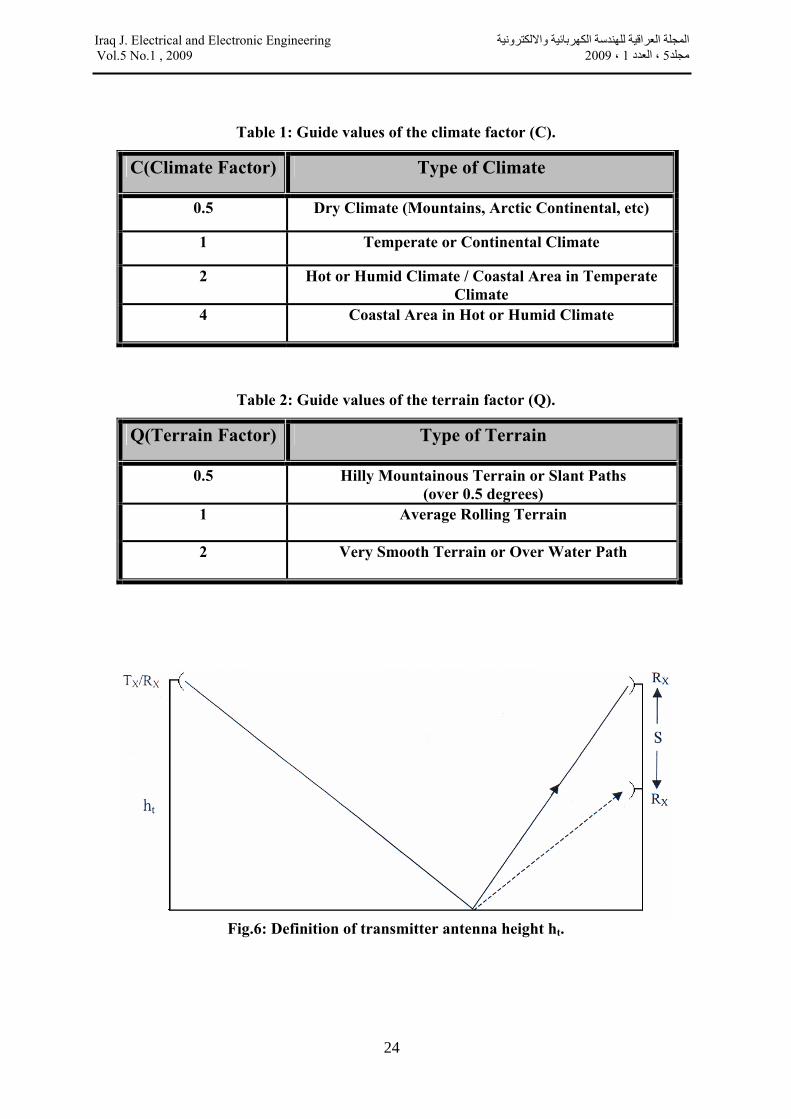
Table 1: Guide values of the climate factor (C).

C(Climate Factor) Type of Climate

0.5 Dry Climate (Mountains, Arctic Continental, etc)

1 Temperate or Continental Climate

2 Hot or Humid Climate / Coastal Area in Temperate Climate

4 Coastal Area in Hot or Humid Climate

Table 2: Guide values of the terrain factor (Q).

Q(Terrain Factor) Type of Terrain

0.5 Hilly Mountainous Terrain or Slant Paths (over 0.5 degrees)

1 Average Rolling Terrain

2 Very Smooth Terrain or Over Water Path

Fig.6: Definition of transmitter antenna height ht.


24

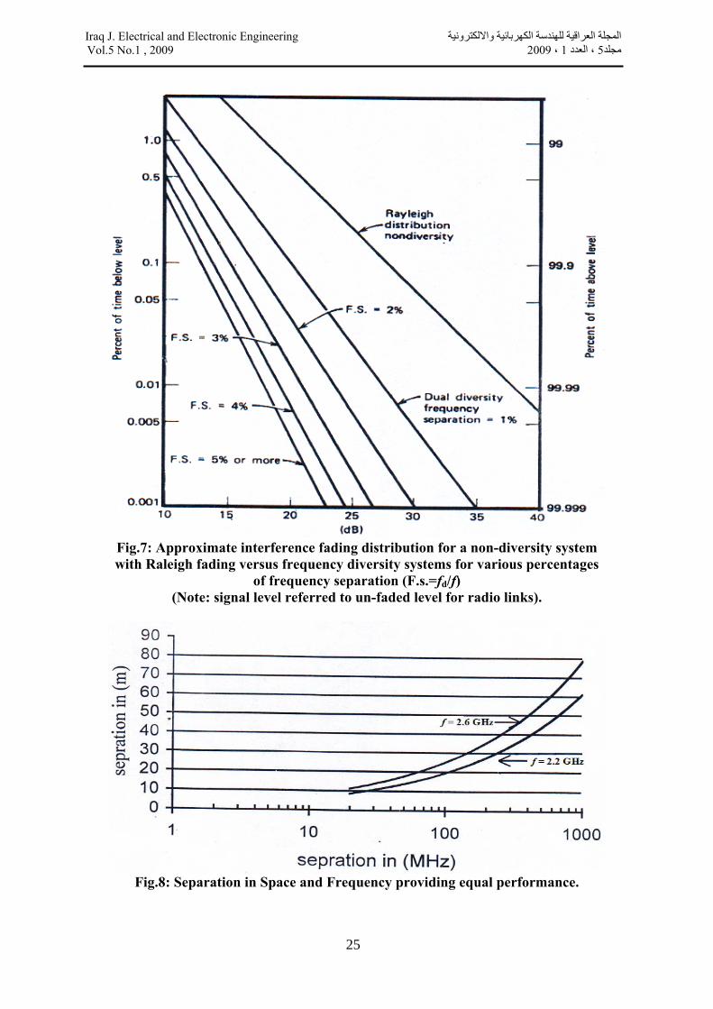
Fig.7: Approximate interference fading distribution for a non-diversity system with Raleigh fading versus frequency diversity systems for various percentages

of frequency separation (F.s.=fd/f) (Note: signal level referred to un-faded level for radio links).

Fig.8: Separation in Space and Frequency providing equal performance.


25

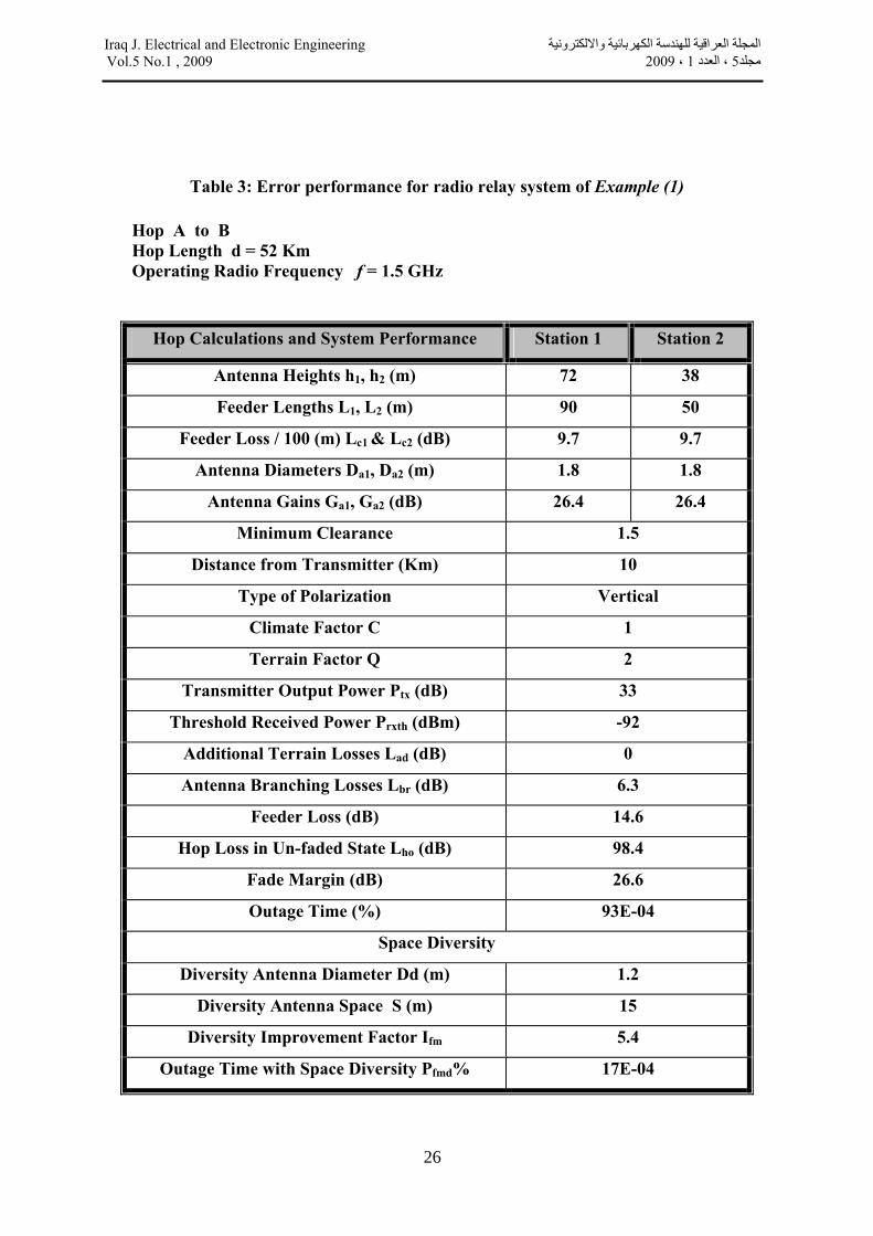
Table 3: Error performance for radio relay system of Example (1)

Hop A to B Hop Length d = 52 Km Operating Radio Frequency f = 1.5 GHz

Hop Calculations and System Performance Station 1 Station 2

Antenna Heights h1, h2 (m) 72 38

Feeder Lengths L1, L2 (m) 90 50

Feeder Loss / 100 (m) Lc1 & Lc2 (dB) 9.7 9.7

Antenna Diameters Da1, Da2 (m) 1.8 1.8

Antenna Gains Ga1, Ga2 (dB) 26.4 26.4

Minimum Clearance 1.5

Distance from Transmitter (Km) 10

Type of Polarization Vertical

Climate Factor C 1

Terrain Factor Q 2

Transmitter Output Power Ptx (dB) 33

Threshold Received Power Prxth (dBm) -92

Additional Terrain Losses Lad (dB) 0

Antenna Branching Losses Lbr (dB) 6.3

Feeder Loss (dB) 14.6

Hop Loss in Un-faded State Lho (dB) 98.4

Fade Margin (dB) 26.6

Outage Time (%) 93E-04

Space Diversity

Diversity Antenna Diameter Dd (m) 1.2

Diversity Antenna Space S (m) 15

Diversity Improvement Factor Ifm 5.4

Outage Time with Space Diversity Pfmd% 17E-04


26

Table 4: Error performance for radio relay system of Example (2)

Hop REP1 to REP2 Hop Length d = 43 Km Operating Radio Frequency f = 2.2 GHz

Hop Calculations and System Performance Station 1 Station 2

Antenna Heights h1, h2 (m) 25 25

Feeder Lengths L1, L2 (m) 30 30

Feeder Loss / 100 (m) Lc1 & Lc2 (dB) 3.8 3.8

Antenna Diameters Da1, Da2 (m) 2.4 2.4

Antenna Gains Ga1, Ga2 (dB) 32.3 32.3

Minimum Clearance -34.1715

Distance from Transmitter (Km) 21.4996

Type of Polarization Vertical

Climate Factor C 2

Terrain Factor Q 1

Transmitter Output Power Ptx (dB) 21.8

Threshold Received Power Prxth (dBm) -81.2

Additional Terrain Losses Lad (dB) 25.2995

Antenna Branching Losses Lbr (dB) 6.8

Feeder Loss (dB) 3.28

Hop Loss in Un-faded State Lho (dB) 102.7974

Fade Margin (dB) 0.2026

Outage Time (%) 3.065

Msm -

Outage Time Due to Selective Multipath Fading Psm % 0


27

a simplified -a final copy

Documents