a simulated annealing algorithm to determine a group

A Simulated Annealing Algorithm to Determine a Group Layout and Production Plan in a Dynamic Cellular Manufacturing System

Reza Kiaa,*, Nikbakhsh Javadianb, Reza Tavakkoli-Moghaddamc aPhD Student, Department of Industrial Engineering, Mazandaran University of Science & Technology, Babol, Iran

b Assistant Professor, Department of Industrial Engineering, Mazandaran University of Science & Technology, Babol, Iran c Professor, School of Industrial Engineering, College of Engineering, University of Tehran, Tehran, Iran

Received 4 March, 2013; Revised 19 May, 2013; Accepted 5 August, 2013

Abstract

In this paper, a mixed-integer linearized programming (MINLP) model is presented to design a group layout (GL) of a cellular manufacturing system (CMS) in a dynamic environment and considering production planning (PP) decisions. This model incorporates an extensive coverage of important manufacturing features used in the design of CMSs. There are also some features that make the presented model different from the previous studies. These include: 1) the variable number of cells, 2) machine depot keeping idle machines, and 3) integration of cell formation (CF), GL and PP decisions in a dynamic environment. The objective is to minimize the total costs (i.e., costs of intra-cell and inter-cell material handling, machine relocation, machine purchase, machine overhead, machine processing, forming cells, outsourcing and inventory holding). Two numerical examples are solved by the GAMS software to illustrate the results obtained by the incorporated features. Since the problem is NP-hard, an efficient simulated annealing (SA) algorithm is developed to solve the presented model. It is then tested using several test problems with different sizes and settings to verify the computational efficiency of the developed algorithm in comparison to the GAMS software. The obtained results show that the quality of the solutions obtained by SA is entirely satisfactory compared to GAMS software based on the objective value and computational time, especially for large-sized problems. Keywords: Dynamic cellular manufacturing systems;Ggroup layout; Production planning; Simulated annealing.

1. Introduction

Setup time reduction, work-in-process inventory reduction, material handling cost reduction, machine utilization improvement, and quality improvement are some the benefits of Cellular Manufacturing (CM) implementation. The design steps of a cellular manufacturing system (CMS) involves 1) cell formation (CF) (i.e., grouping parts with similar processing requirements into part families and corresponding machines into machine cells), 2) group layout (GL) (i.e., placing machines within each cell, called intra-cell layout, and cells in connection with one another, called inter-cell layout), 3) group scheduling (GS) (i.e., scheduling part families), and 4) resource allocation (i.e., assigning tools, human and material resources) (Wemmerlov and Hyer, 1986).

This paper focuses on the first and second stages of the CM design (i.e., cell formation and group layout problems) under a dynamic environment. In a dynamic environment, the product mix and part demands vary during a multi-period planning horizon and necessitate reconfigurations of cells to form cells efficiently for

successive periods. This type of model is called the dynamic cellular manufacturing system (DCMS) (Rheault et al. 1995).

For the first time, Rosenblatt (1986) introduced a model and developed a dynamic programming approach for the dynamic layout problem (DLP), where it is assumed that facilities can be easily relocated. The optimal location of each facility in each manufacturing period is investigated to be obtained by minimizing the total costs of material handling and machine relocation (Baykasoglu and Gindy, 2001). Drolet et al. (2008) developed a stochastic simulation model and indicated that DCMSs are generally more efficient than classical CMSs or job shop systems, especially with respect to performance measures (e.g., throughput time, work-in-process, tardiness and the total marginal cost for a given horizon).

Since a comprehensive literature review related to layout problems and dynamic issues in designing a CMS has been done by Kia et al. (2012 and 2013), we only mention some recent studies implemented in the area of DCMS. Javadi et al. (2013) presented a comprehensive model for the cell formation and group layout design. The

* Corresponding author E-mail: [email protected]

Journal of Optimization in Industrial Engineering 14 (2014) 37-52

37

proposed model incorporated an extensive coverage of important operational features and layout design aspects to design intra and inter-cell layout and material handling flow path structure simultaneously. They examined the benefits of incorporated features including routing flexibility, operation sequence, variable number of cells, un-equal area machines, machines and cells with free orientation, and pickup and drop off station for each cell. The obtained results illustrated that an integrated approach in CMS design can improve the quality of the obtained solution.

Wu et al. (2007) developed a hierarchical genetic algorithm (GA) to simultaneously identify manufacturing cells and the group layout. Jolai et al. (2011) considered CMS formation and layout problems and developed an Electromagnetism like (EM-like) algorithm to minimize the cost of handling and number of exceptional elements.

Saidi-Mehrabad and Safaei (2007) presented the dynamic cell formation model, in which the number of formed cells at each period can be different. Saidi-Mehrabad and Mirnezami-Ziabari (2011) presented a multi-objective mixed integer model to 1) minimize total costs of human resource reassignment, the inter-cell material handling, machine constant and variable, machine relocation and machine purchase, 2) minimize cell load imbalances and 3) maximize utilization rate of human resource. Particle swarm optimization was employed to solve the model.

Defersha and Chen (2006) proposed a comprehensive mathematical model incorporating dynamic cell configuration, alternative routings, lot splitting, sequence of operations, multiple units of identical machines, machine capacity, workload balancing among cells, operation cost, subcontracting cost, tool consumption cost, setup cost, cell size limits, and machine adjacency constraints. Safaei et al. (2008) developed a mixed-integer programming model considering the batch inter and intra-cell material handling by assuming the sequence of operations, alternative process plans, and machine replication to design the CMS under a dynamic environment.

Ahkioon et al. (2009) presented a mixed-integer programming approach for designing a DCMS with multi-period Production Planning (PP), cell reconfiguration, operation sequence, duplicate machines, machine capacity and machine procurement as well as the introduction of the routing flexibility. Safaei and Tavakkoli-Moghaddam (2009) investigated the effect of the trade-off between internal production and outsourcing costs on the cell reconfiguration by integrating the multi-period cell formation and production planning in a DCMS in order to minimize the costs of machine, inter/intra-cell movement, reconfiguration, subcontracting and inventory holding.

Kamali-Dolat-Abadi (2010) developed a model generating the cells and location facilities at the same time with ability of moving the machine(s) from one cell to another cell and generating the new cells for each

period in a dynamic environment. A GA was used for solving the problem. Mahdavi et al. (2010) presented an integer non-linear mathematical programming model for the design of DCMSs with consideration of multi-period production planning, dynamic reconfiguration, operation time, production volume of parts, machine capacity, alternative workers, hiring and firing of workers, and worker assignment.

Rafiee et al. (2011) presented a comprehensive mathematical model for integrated cell formation and inventory lot sizing problem to minimize the total cost of machine procurement, cell reconfiguration, preventive and corrective repairs, material handling (intra-cell and inter-cell), machine operation, part subcontracting, finished and unfinished parts inventory, and defective parts replacement. Saxena and Jain (2011) proposed a DCMS model considering machine breakdown effect to incorporate reliability issue, production planning, and design features including process batch size, transfer batch size, lot splitting, alternative process routing, sequence of operation, machine duplicates, machine capacity, work load balancing, machine procurements and cell reconfiguration.

For the first time, group layout design of a DCMS was presented by Kia et al. (2012) with a novel mixed-integer non-linear programming model. The disadvantage of their work was that the number of cells which should be formed in each period was predetermined by system designer. In an extended study, a multi-objective model which could find the optimal number of cells was formulated by Kia et al. (2013). The advantage of the proposed model in compare to the previous study by Kia et al. (2012) was considering the optimal number of cells in a multi-objective model with two conflicting objectives that minimized the total costs and minimize the imbalance of workload among cells.

The model presented in this study is an extended version of the multi-objective model proposed by Kia et al. (2013), whose advantages include: (1) multi-rows layout of equal-sized facilities, (2) flexible configuration of cells, (3) calculating relocation cost based on the locations assigned to machines, (4) distance-based calculation of intra- and inter-cell material handling costs, (5) considering intra-cell movements between two machines of a same type, (6) applying the equations of material flow conservation, (7) integrating the CF and GL decisions in a dynamic environment, and (8) finding the optimal number of cells. An obvious drawback in their work was that a metaheuristic approach was not designed for solving large-sized problems. To overcome this disadvantage, a simulated annealing approach is designed to solve the problem with a single objective. Also, machine depot feature and PP decisions are added to the previous model to enhance its flexibility in handling changing demand.

The aims of this study are twofold. The first one is to present a new mathematical model with an extensive coverage of important manufacturing features consisting

Reza Kia et al./ A Silmulated Annealing Algorithm to...

38

of alternate process routings, operation sequence, processing time, production volume of parts, purchasing machine, duplicate machines, machine capacity, machine depot, lot splitting, group layout, multi-rows layout of equal area facilities, flexible reconfiguration of cells, variable number of cells, outsourcing and inventory holding of parts. The second aim is to develop an efficient simulated annealing algorithm to solve the presented model.

In this paper, an efficient SA approach is developed for solving the presented model, because it belongs to NP-hard problems. Two numerical examples are solved by the GAMS software to illustrate advantages of the presented model. Additionally, several numerical examples are solved using the extended SA to verify the efficiency of the developed algorithm. Furthermore, the efficiency of designed SA algorithm in terms of both the objective value and computational time is shown by comparing our results to those found in examples solved by GAMS software.

The remainder of this paper is organized as follows. In Section 2, a mathematical model integrating DCMS, GL and PP decisions is presented. We develop the SA algorithm in Section 3. Section 4 solves the test problems in order to investigate the features of the presented model and shows the performance of the developed algorithm. Finally, this paper ends with conclusions in Section 5.

2. Mathematical model and problem descriptions

2.1. Model assumptions

In this section, the DCMS model integrating GL and PP is formulated under a number of assumptions. Some of these assumptions are the same as those considered by Kia et al. (2012). However, the new assumptions are considered below: 1. The overhead cost of each machine type implying

maintenance and other overhead costs such as energy cost and general service is known. This cost would be considered for each machine in each period only if that machine was utilized on the cells to process part-operations.

2. It is assumed that in the first period, there is no machine available to be utilized. Hence, in the first period it would be needed to purchase some machines to meet part demands. In the next periods, if the present time capacity of machines was not enough to satisfy the part demands, some other machines would be purchased and added to the current utilized machines.

3. In each period that there is surplus capacity, idle machines can be removed from the cells and transferred to the machine depot, where the idle machines are kept in order to decrease the machine overhead costs and provide empty locations in cells to accommodate required machines. Whenever it would

be necessary to increase the processing time capacity of the system because of high demand volume, those machines could be returned to the cells.

4. Cell reconfiguration involves different situations which are: 1) transferring of the existing machines between different locations of a same cell or different cells, 2) purchasing and adding new machines to cells, and 3) transferring machines between cells and the machine depot because of changing capacity requirements in successive periods.

5. The relocation cost of each machine type between two periods is known. All machine types can be moved to the machine depot or any location in the cells. Even if a machine is removed from or returned to the cells, this relocation cost is incurred. This cost is paid for several situations: 1) to install a new purchased machine or a machine returned from the machine depot, 2) to uninstall a machine removed from a cell to be kept in the machine depot, and 3) to transfer a machine between two different locations of a same cell or different cells. Transferring machine contains uninstallation of a machine from a location and installation of that machine in another location. Installing and uninstalling costs are considered to be same. Actually, if a machine which has been newly purchased or returned from the machine depot is added to a cell, the only installing cost will be imposed. In the same way, if a machine is removed from a cell to be kept in the machine depot, the only uninstalling cost will be incurred. Then, if a machine is transferred between two different locations in the cells, both uninstalling and installing costs will be imposed. Thus, it would be reasonable to assume that the unit cost of adding or removing a machine to/from the cells is half of relocation machine cost.

6. Obviously, the maximum number of machines which can be present in a period is equal to the number of locations. Therefore, the maximum number of cells which can be formed is determined by:

퐶 =푡ℎ푒푛푢푚푏푒푟표푓푙표푐푎푡푖표푛푠푙표푤푒푟푏표푢푛푑표푓푐푒푙푙푠푖푧푒

However, the number of cells which should be formed in each period is considered as a decision variable in our model.

7. Depending on the fluctuations of demand volumes and total costs of meeting those demands, the system can produce some surplus parts in a period, hold as an inventory between successive periods and used in the future planning periods. Also, due to limited machine capacities, outsourcing can be used to provide some of the required parts to meet the market demand. The following notations are used in the model:


39

2.1.1. Sets

P = {1,2,… , 푃} index set of part types K(p) = 1,2,… ,퐾

index set of operations indices for part type p

M = {1,2,… ,푀} index set of machine types C = {1,2,… , 퐶} index set of cells L = {1,2,… , 퐿} index set of locations T = {1,2,… , 푇} index set of time periods

2.1.2. Model parameters 퐼퐸 inter-cell material handling cost per part type p

per unit of distance

퐼퐴 intra-cell material handling cost per part type p per unit of distance

훿 relocation cost per machine type m 퐷 demand for part type p in period t 푇 capacity of one unit of machine type m

퐶 maximum number of cells that can be formed in each period

퐹퐶 cost of forming a cell in period t 퐵 upper cell size limit 퐵 lower cell size limit

푡 processing time of operation k on machine m per part type p

푑 distance between two locations l and l’ 훼 overhead cost of machine type m in each period 훽 variable cost of machine type m for each unit time 훾 purchase cost of machine type m 푂퐶 outsourcing cost per unit part type p 퐻퐶

inventory holding cost per unit part type p during each period

푎

= 10ifoperation푘ofpart푝canbeprocessedonmachineotherwise

2.1.3. Decision variables 푋 number of parts of type p processed by

operation k on machine type m assigned to location l in period t

푌 1 if cell c is formed in period t; 0, otherwise 푊 1 if one unit of machine type m is assigned to

location l and assigned to cell c in period t; 0, otherwise

푌 ′ ′ number of parts of type p processed by operation k on machine type m assigned to location l and moved to the machine type m’ assigned to location l’ in period t

푁 number of machine type m purchased in period t

푁 number of machine type m removed from the machine depot and returned to cells in period t

푁 number of machine type m removed from cells

and moved to the machine depot in period t 푂 number of part type p to be outsourced in

period t 푉 inventory quantity of part type p kept in period

t and carried over to period t+1

2.2. Mathematical model

The developed DCMS model is now formulated as a mixed-integer non-linear programming model:

min푍 = 푊

×푊 × 푌 × 푑× 퐼퐴

(1.1)

+ 푊

×푊 × 푌× 푑 × 퐼퐸

(1.2)

+12 훿 ×푊 ,

+12 훿

× 푊

− 푊 ,

(1.3)

+ 훾 .푁 (1.4)

+ 훼 × 푊 (1.5)

+ 훽 × 푡 × 푋 (1.6)

퐹퐶 . 푌 (1.7)

푂퐶 . 푂 (1.8)

퐻퐶 .푉 (1.9)

s.t.

푋 ≤ 푀.푎 ∀푘 ∈ 퐾푝, ∀푝 ∈ 푃,∀푚∈ 푀, ∀푙 ∈ 퐿, ∀푡 ∈ 푇 (2)


40

퐷

= 푋 ,

+ 푉 − 푉 +푂

∀푝 ∈ 푃,∀푡 ∈ 푇 (3)

푊

= 푊

+푁 +푁 −푁

∀푚 ∈ 푀, ∀푡 ∈ 푇 (4)

푁

≤ 푁 − 푁 ∀푚 ∈ 푀, 푡 = 3,… , 푇 (5)

푊 ≤ 퐿 ∀푡 ∈ 푇 (6)

푊

≤ 퐵 . 푌

∀푐 ∈ 퐶, ∀푡 ∈ 푇 (7)

퐵 × 푌

≤ 푊 ∀푐 ∈ 퐶, ∀푡 ∈ 푇 (8)

푌( ) ≤ 푌 ∀푐 ∈ 퐶 − 1, ∀푡 ∈ 푇 (9)

푋 × 푡

≤ 푇 푊

∀푚 ∈ 푀, ∀푙 ∈ 퐿, ∀푡∈ 푇 (10)

푋

= 푌 ∀푘 ∈ 퐾푝, ∀푝 ∈ 푃,∀푚∈ 푀, ∀푙 ∈ 퐿, ∀푡 ∈ 푇 (11)

푋

= 푌 ∀푘 ∈ 퐾푝, ∀푝 ∈ 푃,∀푚′∈ 푀, ∀푙 ∈ 퐿, ∀푡 ∈ 푇 (12)

푊 ≤ 1 ∀푙 ∈ 퐿, ∀푡 ∈ 푇 (13)

푋

≥ 0, 푌

≥ 0andinteger

∀푘 ∈ 퐾푝, ∀푝 ∈ 푃,∀푚,푚

∈ 푀, ∀푙, 푙 ∈ 퐿, ∀푡 ∈ 푇 (14)

푊 ,푌 ,∈ {0, 1} ∀푚 ∈ 푀, ∀푐 ∈ 퐶, ∀푙∈ 퐿, ∀푡 ∈ 푇 (15)

푁 ,푁 ,푁 ,푂 , 푉≥ 0andinteger

∀푝 ∈ 푃,∀푚 ∈ 푀,∀푡∈ 푇 (16)

The objective function consists of nine cost

components. Term (1.1) is the intra-cell material handling cost. This cost is incurred if consecutive operations of the

same part type are processed in the same cell, but on different machines. In a similar way, Term (1.2) denotes the inter-cell material handling cost. This cost is incurred whenever consecutive operations of the same part type are transferred between different cells. In a similar way, Term (1.2) denotes the inter-cell material handling cost. This cost is incurred whenever consecutive operations of the same part type are transferred between different cells. Term (1.3) represents the cost of reconfiguration of cells occurring in 1) installing a new purchased machine or a machine returned from the machine depot, or 2) uninstalling a machine removed from a cell to be kept in the machine depot, or 3) transferring a machine between two locations in the cells. Term (1.4) is the purchase costs of new machines. Term (1.5) incorporates the overhead costs which are paid only for utilized machines in the cells. Term (1.6) takes into account the operating costs of all machine types. Term (1.7) is the total costs of forming cells. Terms (1.8) and (1.9) are for outsourcing and inventory holding costs.

Inequality (2) guarantees that each operation of a part is processed on the machine which is capable to process that operation. Constraint (3) shows that demand of each part can be satisfied in a period through internal production or external outsourcing or inventory carried from the previous period or each combined strategy of these PP decisions leading to optimal plan. Equation (4) describes that the number of machine type m utilized in the period t is equal to number of utilized machines of the same type in the previous period plus the number of new machines of the same type purchased at the beginning of the current period, plus the number of machines of the same type removed from the machine depot and returned to the cells or minus the number of machines of the same type removed from the cells and moved to the machine depot at the beginning of the current period. Inequality (5) ensures that the number of machine type m which can be returned from the machine depot to the cells does not exceed from the number of machine type m available in the machine depot in each period. It is worth mentioning that returning machines from the machine depot to cells can be started in the third period, because before that period there is no any machines in the machine depot. Inequality (6) necessitates that the number of machines of all types utilized in the cells is less than the number of available locations. The cell size is limited through Constraints (7) and (8), where the cell size lies within the user defined lower and upper bounds. Obviously machines can be assigned to a cell only if that cell is formed. The order of forming cells is determined by Constraint (9). Constraint (10) is related to the machine capacity. If machine type m is assigned to location l in cell c, then different part types can process their operations on this machine providing that not exceeding from the time capacity of that machine. Constraints (11) and (12) are material flow conservation equations. Constraint set (13) is to ensure that each location can receive one machine at most and only belong to one cell, simultaneously.


41

Constraints (14)-(16) provide the logical binary and non-negativity integer necessities for the decision variables.

The proposed model is a mixed-integer nonlinear programming model because of the product of decision variables in Expressions (1.1) and (1.2) and absolute term in Expressions (1.3). The linearization of these expressions is done in a way similar to that developed by Kia et al. (2012).

Since in our integrated model, part routings, outsourcing demand, holding inventory, forming cells, machine relocation and group layout decisions are made in a dynamic environment, we actually incorporate a DLP, production planning (PP) and group layout in a DCMS model. In this case, an appropriate decision should be made among the available strategies (e.g., purchasing a new machine to meet increased demand requirements, relocating the machine that is underutilized in a cell to another cell where demand requirements are higher, keeping machines that are underutilized in a depot to reduce the overhead costs, outsourcing parts when internal production is not practical or economical, producing more parts in a period with lower level of demand and holding for the next period with lower level of demand, re-routing the part production due to changing demands, and opening or closing cells order to make a trade-off among resultant costs of purchasing new machines, machine relocation, machine overhead, opening or closing manufacturing cells, internal production, outsourcing, inventory holding and material handling including intra-cell, inter-cell and inter-floor).

3. The simulated annealing algorithm for DCMS

Kirkpatrick et al. (1983) introduced the simulated annealing (SA) algorithm as a stochastic neighborhood search technique for solving hard combinatorial optimization problems. SA emulates the annealing process which attempts to force a system to its lowest energy through controlled cooling. In general, the annealing process is as follows: 1) the temperature is raised to a sufficient level, 2) the temperature is maintained in each level for sufficient time, and 3) the temperature is allowed to cool under controlled conditions until the desired energy is reached. It has been used to many optimization problems in a wide variety of areas, including dynamic cellular manufacturing systems (Kia et al. 2012; Majazi Dalfard, 2013; Tavakkoli-Moghaddam et al. (2008), Safaei et al. 2008; Defersha and Chen, 2009, Defersha and Chen, 2008; Mungwattana, 2000 ). In this section, the SA algorithm is developed to solve the presented model.

3.1. Solution representation

A solution schema proportional to the integrated DCMS model for determining group layout and production planning consists of seven ingredients in each

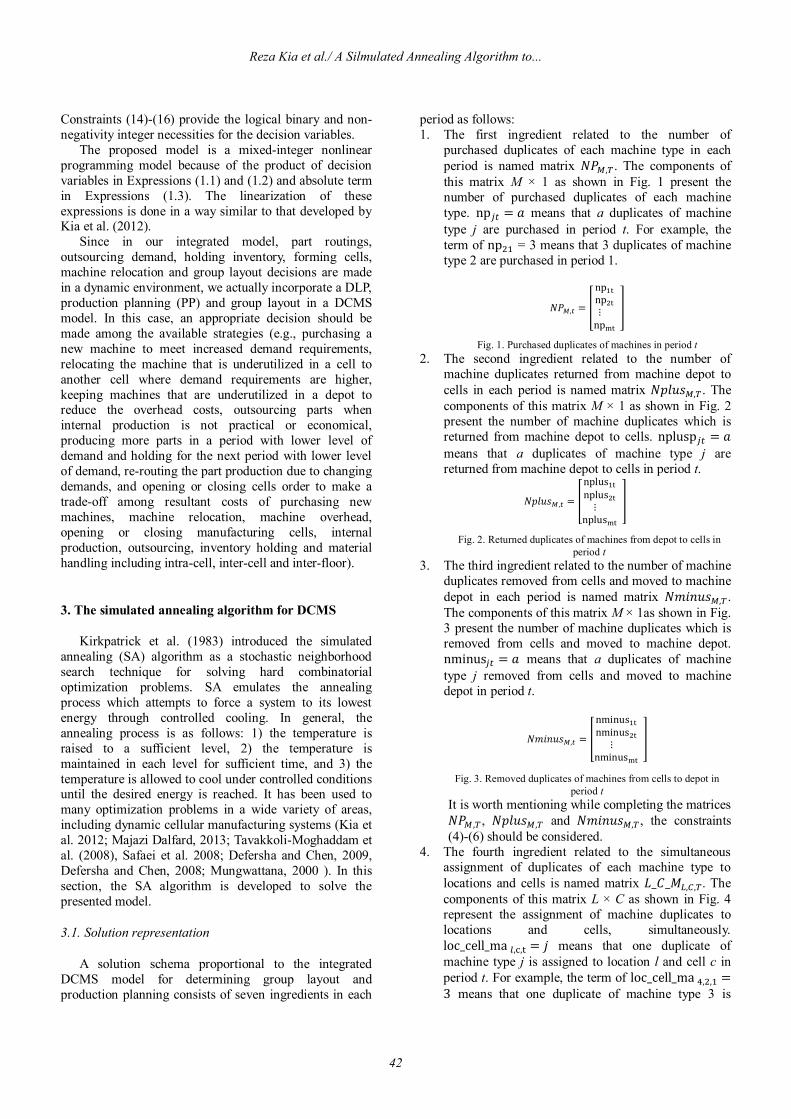
period as follows: 1. The first ingredient related to the number of

purchased duplicates of each machine type in each period is named matrix 푁푃 , . The components of this matrix M × 1 as shown in Fig. 1 present the number of purchased duplicates of each machine type. np = 푎 means that a duplicates of machine type j are purchased in period t. For example, the term of np = 3 means that 3 duplicates of machine type 2 are purchased in period 1.

푁푃 , =

np np ⋮np

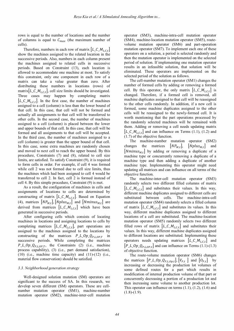
Fig. 1. Purchased duplicates of machines in period t 2. The second ingredient related to the number of

machine duplicates returned from machine depot to cells in each period is named matrix 푁푝푙푢푠 , . The components of this matrix M × 1 as shown in Fig. 2 present the number of machine duplicates which is returned from machine depot to cells. nplusp = 푎 means that a duplicates of machine type j are returned from machine depot to cells in period t.

푁푝푙푢푠 , =

nplus nplus ⋮

nplus

Fig. 2. Returned duplicates of machines from depot to cells in period t

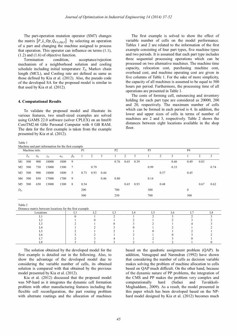
3. The third ingredient related to the number of machine duplicates removed from cells and moved to machine depot in each period is named matrix 푁푚푖푛푢푠 , . The components of this matrix M × 1as shown in Fig. 3 present the number of machine duplicates which is removed from cells and moved to machine depot. nminus = 푎 means that a duplicates of machine type j removed from cells and moved to machine depot in period t.

푁푚푖푛푢푠 , =

nminus nminus

⋮nminus

Fig. 3. Removed duplicates of machines from cells to depot in period t

It is worth mentioning while completing the matrices 푁푃 , , 푁푝푙푢푠 , and 푁푚푖푛푢푠 , , the constraints (4)-(6) should be considered.

4. The fourth ingredient related to the simultaneous assignment of duplicates of each machine type to locations and cells is named matrix 퐿_퐶_푀 , , . The components of this matrix L × C as shown in Fig. 4 represent the assignment of machine duplicates to locations and cells, simultaneously. loc_cell_ma , , = 푗 means that one duplicate of machine type j is assigned to location l and cell c in period t. For example, the term of loc_cell_ma , , =3 means that one duplicate of machine type 3 is


42

assigned to location 4 and cell 2 in period 1. While completing the matrix 퐿_퐶_푀 , , , Constraints (6), (7), (8) and (13) should be satisfied. After completing the matrices 푁푃 , and 퐿_퐶_푀 , , for the entire periods, the values of 푁푝푙푢푠 , and 푁푚푖푛푢푠 , can be derived from Equation (4) in each period.

퐿_퐶_푀 , , =loc_cell_ma , , ⋯ loc_cell_ma , ,

⋮ ⋱ ⋮loc_cell_ma , , ⋯ loc_cell_ma , ,

Fig. 4. Assignment of machine duplicates to locations and cells

5. The fifth ingredient presenting the quantity of part operations assigned to the duplicates of each machine

type assigned to locations is named matrix 푃_퐿_푂푝_푄 , , , . This is a three-dimensional matrix P × L as shown in Fig. 5, in which each component contains k arrays (k is max 퐾 ) presenting the assignment of part operations to locations. 푤 = 푎 means that a quantities of part type p are processed by operation 푘 on the machine assigned to location l. For example, the term of 푤 , , = 100 means that 100 quantities of part type 2 are processed by operation 3 on the machine assigned to location 1. While completing the matrix 푃_퐿_푂푝_푄 , , , , Constraints (2) and (10)–(12) should be satisfied.

푃_퐿_푂푝_푄 , , , =

⎣⎢⎢⎢⎢⎢⎢⎢⎡ 푤 , , 푤 , , …푤 , , … 푤 , , 푤 , , …푤 , , … 푤 , , 푤 , , …푤 , ,

푤 , , 푤 , , …푤 , , … 푤 , , 푤 , , …푤 , , … 푤 , , 푤 , , …푤 , , ⋮⋮⋮

푤 , , 푤 , , …푤 , , … 푤 , , 푤 , , …푤 , , … 푤 , , 푤 , , …푤 , , ⋮⋮⋮

푤 , , 푤 , , …푤 , , … 푤 , , 푤 , , …푤 , , … 푤 , , 푤 , , …푤 , , ⎦⎥⎥⎥⎥⎥⎥⎥⎤

Fig. 5. Assignment of part operations to machine duplicates in locations

6. The sixth ingredient indicating the quantity of inventory of parts kept in period t and carried over to period t+1 is named matrix 푉 , . The components of this matrix P × 1 as shown in Fig. 6 represent the quantity of inventory of parts kept between each two periods.v = 푎 means that a quantities of part type p are kept in period t and carried over to period t+1. For example, the term v = 50 means that 50 quantities of part type 3 are kept in period 1 and carried over to period 2.

푉 , =

v v ⋮v

Fig. 6. Quantity of inventory of parts kept between periods

7. The seventh ingredient indicating the quantity of parts outsourced in period t is named matrix 푂 , . The components of this matrix P × 1 as shown in Fig. 7 represent the quantity of outsourced parts in each period.o = 푎 means that a quantities of part type p are outsourced in period t. For example, the term of o = 50 means that 50 quantities of part type 3 are outsourced in period 1.

푂 , =

o o ⋮o

Fig. 7. Quantity of outsourced parts in each period

While completing the matrices 푃_퐿_푂푝_푄 , , , , V , and O , , Equation (3) should to be satisfied.

In general, with combining seven ingredients described above, the solution representation in each

period is obtained as shown in Fig. 8. It is obvious that each solution combining seven ingredients consists of the T structure, where T is the number of periods.

푁푃 , 푁푝푙푢푠 , 푁푚푖푛푢푠 , 퐿, ,

푃_퐿_푂푝_푄 , , , | 푉 , | 푂 ,

Fig. 8. Solution representation in period t

3.2. Generating an initial solution

The initial solution is generated according to a hierarchical approach, in which matrices 퐿_퐶_푀 , , , 푁푃 , , 푁푝푙푢푠 , , 푁푚푖푛푢푠 , , 푃_퐿_푂푝_푄 , , , , 푉 , and 푂 , are constructed sequentially in each

period by the random numbers limited in the determined interval provided that those matrices satisfy corresponding constraints. The generation process of initial solutions is described as follows:

In the first stage, the matrix 퐿_퐶_푀 , , determining how duplicates of each machine type are assigned to locations and cells is constructed. To generate a good initial solution, the number of machines of each type which is required for processing part operations is estimated roughly. This is done by considering parameters 푡 and 퐷 of each part type and randomly selecting a machine capable to process each operation of a part based on parameter 푎 .

Then, the components of matrix 퐿_퐶_푀 , , receive numbers randomly distributed between 1 and M (the number of machine types) for all periods. The number of


43

rows is equal to the number of locations and the number of columns is equal to 퐶 (the maximum number of cells).

Therefore, numbers in each row of matrix 퐿_퐶_푀 , , show the machines assigned to the related location in the successive periods. Also, numbers in each column present the machines assigned to related cells in successive periods. Based on Constraint (13), each location is allowed to accommodate one machine at most. To satisfy this constraint, only one component in each row of a matrix can take a value greater than zero. After distributing these numbers in locations (rows) of matrix 퐿_퐶_푀 , , , cell size limits should be investigated. Three cases may happen by completing matrix 퐿_퐶_푀 , , . In the first case, the number of machines

assigned to a cell (column) is less than the lower bound of that cell. In this case, that cell will not be formed and actually all assignments to that cell will be transferred to other cells. In the second case, the number of machines assigned to a cell (column) is placed between the lower and upper bounds of that cell. In this case, that cell will be formed and all assignments to that cell will be accepted. In the third case, the number of machines assigned to a cell (column) is greater than the upper bound of that cell. In this case, some extra machines are randomly chosen and moved to next cell to reach the upper bound. By this procedure, Constraints (7) and (8), related to cell size limits, are satisfied. To satisfy Constraint (9), it is required to form cells in order. For example, if cell 4 was formed while cell 2 was not formed due to cell size limits, thus the machines which had been assigned to cell 4 would be transferred to cell 2. In fact, cell 2 is formed instead of cell 4. By this simple procedure, Constraint (9) is met.

As a result, the configuration of machines in cells and assignments of locations to cells are determined by constructing of matrix 퐿_퐶_푀 , , . Based on Equation (4), matrices 푁푃 , , 푁푝푙푢푠 , and 푁푚푖푛푢푠 , are derived from matrices 퐿_퐶_푀 , , which have been generated in successive periods.

After configuring cells which consists of locating machines in locations and assigning locations to cells by completing matrices 퐿_퐶_푀 , , , part operations are assigned to the machines assigned to the locations by constructing of the matrices 푃_퐿_푂푝_푄 , , , in successive periods. While completing the matrices 푃_퐿_푂푝_푄 , , , , the Constraints (2) (i.e., machine process capability), (3) (i.e., part demand satisfaction), (10) (i.e., machine time capacity) and (11)-(12) (i.e., material flow conservation) should be satisfied. 3.3. Neighborhood generation strategy

Well-designed solution mutation (SM) operators are

significant to the success of SA. In this research, we develop seven different (SM) operators. These are cell-number mutation operator (SM1), machine-number mutation operator (SM2), machine-inter-cell mutation

operator (SM3), machine-intra-cell mutation operator (SM4), machine-location mutation operator (SM5), route-volume mutation operator (SM6) and part-operation mutation operator (SM7). To implement each one of these operators on a solution, a period is selected randomly and then the mutation operator is implemented on the selected period of solution. If implementing one mutation operator results in an infeasible solution, that solution will be eliminated. These operators are implemented on the selected period of the solution as follows.

The cell-number mutation operator (SM1) changes the number of formed cells by adding or removing a formed cell. By this operator, the only matrix 퐿_퐶_푀 , , is changed. Therefore, if a formed cell is removed, all machine duplicates assigned to that cell will be reassigned to the other cells randomly. In addition, if a new cell is formed, some machine duplicates assigned to the other cells will be reassigned to the newly-formed cell. It is worth mentioning that the part operations processed by the randomly selected machines will be remained with them. Adding or removing a cell needs updating matrix 퐿_퐶_푀 , , and can influence on Terms (1.1), (1.2) and

(1.7) of the objective function. The machine-number mutation operator (SM2)

changes the matrices 푁푃 , , 푁푝푙푢푠 , and 푁푚푖푛푢푠 , by adding or removing a duplicate of a

machine type or concurrently removing a duplicate of a machine type and then adding a duplicate of another machine type. Implementing this operator might need updating all matrices and can influence on all terms of the objective function.

The machine-inter-cell mutation operator (SM3) randomly selects two different filled columns of matrix 퐿_퐶_푀 , , and substitutes their values. In this way,

different machine duplicates assigned to different cells are substituted between cells. The machine-intra-cell mutation operator (SM4) randomly selects a filled column of matrix 퐿_퐶_푀 , , and substitutes its values. In this way, different machine duplicates assigned to different locations of a cell are substituted. The machine-location mutation operator (SM5) randomly selects two different filled rows of matrix 퐿_퐶_푀 , , and substitutes their values. In this way, different machine duplicates assigned to different locations are substituted. Implementing these operators needs updating matrices 퐿_퐶_푀 , , and 푃_퐿_푂푝_푄 , , , and can influence on Terms (1.1)-(1.3)

of objective function. The route-volume mutation operator (SM6) changes

the matrices 푃_퐿_푂푝_푄 , , , , 푉 , and 푂 , by increasing or decreasing the production lot volumes of some defined routes for a part which results in modification of internal production volume of that part or concurrently decreasing a portion of a production lot and then increasing same volume to another production lot. This operator can influence on terms (1.1), (1.2), (1.6) and (1.8)-(1.9).


44

The part-operation mutation operator (SM7) changes the matrix 푃_퐿_푂푝_푄 , , , by selecting an operation of a part and changing the machine assigned to process that operation. This operator can influence on terms (1.1), (1.2) and (1.6) of objective function.

Termination condition, acceptance/rejection mechanism of a neighborhood solution and cooling schedule including initial temperature T0, Markov chain length (MCL), and Cooling rate are defined as same as those defined by Kia et al. (2012). Also, the pseudo code of the developed SA for the proposed model is similar to that used by Kia et al. (2012).

4. Computational Results

To validate the proposed model and illustrate its various features, two small-sized examples are solved using GAMS 22.0 software (solver CPLEX) on an Intel® CoreTM2.66 GHz Personal Computer with 4 GB RAM. The data for the first example is taken from the example presented by Kia et al. (2012).

The first example is solved to show the effect of variable number of cells on the model performance. Tables 1 and 2 are related to the information of the first example consisting of four part types, five machine types and two periods. It is assumed that each part type includes three sequential processing operations which can be processed on two alternative machines. The machine time capacity, relocation cost, purchasing machine cost, overhead cost, and machine operating cost are given in five columns of Table 1. For the sake of more simplicity, the capacity of all machines is assumed to be equal to 500 hours per period. Furthermore, the processing time of all operations are presented in Table 1.

The costs of forming cell, outsourcing and inventory holding for each part type are considered as 20000, 200 and 20, respectively. The maximum number of cells which can be formed in each period is 4. In addition, the lower and upper sizes of cells in terms of number of machines are 2 and 3, respectively. Table 2 shows the distances between eight locations available in the shop floor.

Table 1 Machine and part information for the first example

P4 P3 P2 P1 Machine info.

3 2 1 3 2 1 3 2 1 3 2 1 βm αm γm δm Tm

0.83 0.49 0.46 0.39 0.65 0.76 9 1800 18000 900 500 M1

0.74 0.33 0.99 0.79 7 1500 15000 750 500 M2

0.45 0.57 0.44 0.93 0.73 5 1800 18000 900 500 M3

0.14 0.80 0.46 9 1700 17000 850 500 M4

0.62 0.67 0.48 0.93 0.65 0.54 8 1300 13000 650 500 M5

0 300 700 200 Dpt

300 700 250 500

Table 2 Distance matrix between locations for the first example

Locations L1 L2 L3 L4 L5 L6 L7 L8 L1 0 1 2 1 2 3 2 3 L2 1 0 1 2 1 2 3 2 L3 2 1 0 3 2 1 4 3 L4 1 2 3 0 1 2 1 2 L5 2 1 2 1 0 1 2 1 L6 3 2 1 2 1 0 3 2 L7 2 3 4 1 2 3 0 1 L8 3 2 3 2 1 2 1 0

The solution obtained by the developed model for the

first example is detailed out in the following. Also, to show the advantage of the developed model due to considering the variable number of cells, its obtained solution is compared with that obtained by the previous model presented by Kia et al. (2012).

Kia et al. (2012) discussed that the proposed model was NP-hard as it integrates the dynamic cell formation problem with other manufacturing features including the flexible cell reconfiguration, the part routing problem with alternate routings and the allocation of machines

based on the quadratic assignment problem (QAP). In addition, Venugopal and Narendran (1992) have shown that considering the number of cells as decision variable makes solving the problem of machine allocation to cells based on QAP much difficult. On the other hand, because of the dynamic nature of PP problems, the integration of the CMS and PP makes the problem very complex and computationally hard (Safaei and Tavakkoli-Moghaddam., 2009). As a result, the model presented in this paper which has been developed based on the NP-hard model designed by Kia et al. (2012) becomes much


45

complicated by incorporating variable number of cells and PP decisions.

The optimal solution is obtained after 74159 seconds (i.e., about 20 hours) for the first example which consists of 652,619 variables and 751,238 constraints. This implies the NP-hardness of the proposed model even in solving such a small-sized example. The cell configurations, machine layout and material flow for two periods corresponding to the best solutions obtained using the model presented by Kia et al. (2012) with three cells and the proposed model in this paper with two optimal cells are shown in Tables 3 and 4, respectively. These tables show the advantage of the proposed model with variable number of cells. As can be seen, in the optimal solution of the developed model with variable number of cells, two cells in each period are formed. This reduces the forming cost of cells in the developed model compared with the previous model where forming three cells had been predetermined by system designer. It is worth mentioning that in the optimal solution for the developed model, the demands of all parts in each period are satisfied by internal production in the same period and outsourcing demand and holding inventories between periods are not economic. As a result, the cost components related to outsourcing and inventory holding are equal to zero in the optimal objective function value (OFV).

Here, the OFV obtained in this paper is compared to the previous study carried out by Kia et al. (2012). In order to make a fair comparison between the OFVs of two mathematical models, they should have same components. Therefore, the costs of forming cells, outsourcing and inventory holding should be added to the OFV of the previous study. Since outsourcing and inventory holding were not considered in the previous

study, the only cost component remaining to be added to Table 5 is the forming cell cost. The optimal OFV and cost components for the first example obtained by the previous study with three cells and the developed model with 2 cells (i.e., the optimal number of formed cells) are presented in Tables 5 and 6, respectively.

Since the number of cells which should be formed is predetermined to 3 in the previous study, then the cost of forming three cells in two periods is equal to 3×2×20000=120000. However, in the developed model, the number of cells which should be formed is considered as a decision variable due to finding the optimal number of cells. The optimal number of cells formed in each period is equal to 2. This causes the cost of forming cell takes the value equal to 2×2×20000=80000. By comparing forming cell cost component of two models, it can be understood the developed model reduces the forming cell cost through finding the optimal number of formed cells. This reduction is equal to 120000-80000=40000 (i.e., (40000/252812.7)×100=15%) which is a promising result. Also, in the optimal solution of the developed model, 6 machines are purchased in the first period and utilized for both periods. However, in the optimal solution of the previous model, 7 machines are purchased and utilized in two successive periods. Purchasing fewer machines results in reduction of costs of machine purchase and machine overhead. This reduction is equal to (114000+21300)-(94000-18800)=225000 (i.e., (22500/252812.7)×100=9%) which reveals another capability of the proposed model to reduce the total costs of forming cell, machine purchase and machine overhead through forming cells in optimal numbers.

Table 3 Machine locations and part-operation allocations to the machines for the first example with predetermined number of cells (three cells in each period).

P4 P3 P2 P1 Machine info 3 2 1 3 2 1 3 2 1 3 2 1 L M C 352 146 352 7 M1 C1 206 4 M5 200 1 M2 C2 3 M2 200 200 2 M3 300 348 348 8 M1 C3 300 300 348 5 M4

P4 P3 P2 P1 Machine info

3 2 1 3 2 1 3 2 1 3 2 1 L M C 273 700 105 26 3 M2

C1 273 273 79 105 2 M3 700 700 6 M4 27 395 395 1 M2 C2 27 27 395 4 M5 7 M1 C3 250 250 250 8 M1

Period 1

Period 2


46

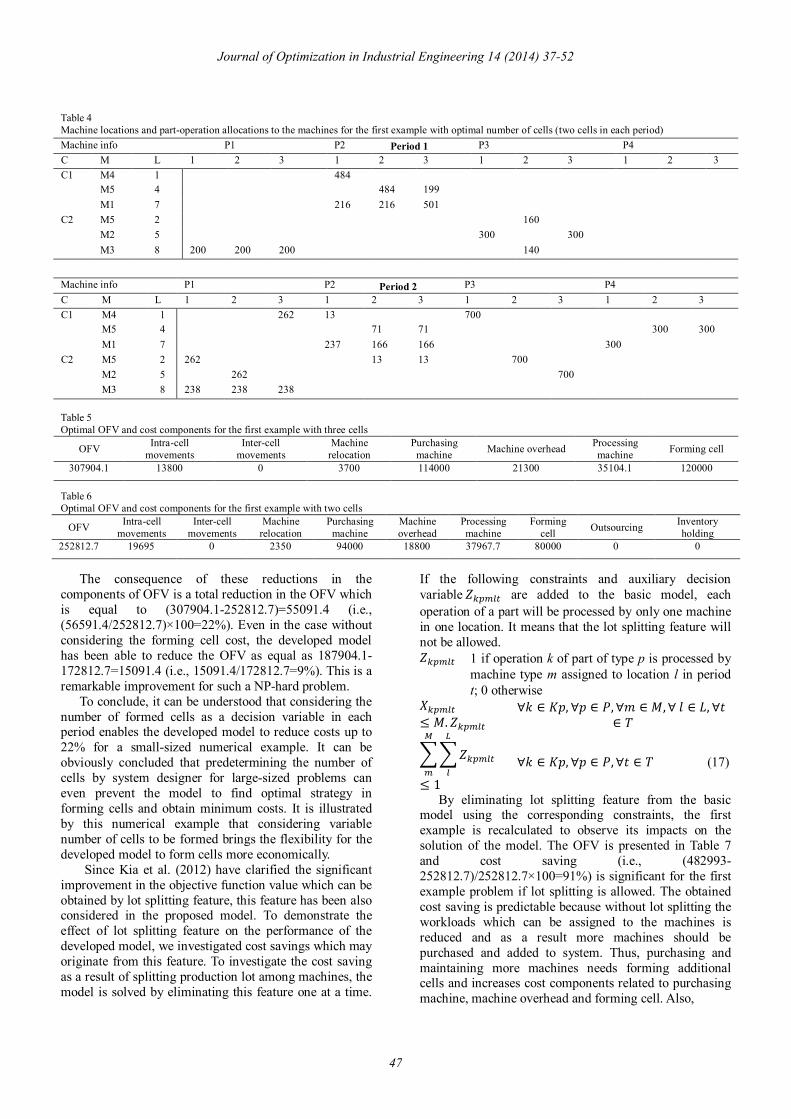
Table 4 Machine locations and part-operation allocations to the machines for the first example with optimal number of cells (two cells in each period)

P4 P3 P2 P1 Machine info 3 2 1 3 2 1 3 2 1 3 2 1 L M C 484 1 M4 C1 199 484 4 M5 501 216 216 7 M1 160 2 M5 C2 300 300 5 M2 140 200 200 200 8 M3

P4 P3 P2 P1 Machine info

3 2 1 3 2 1 3 2 1 3 2 1 L M C 700 13 262 1 M4 C1

300 300 71 71 4 M5 300 166 166 237 7 M1 700 13 13 262 2 M5 C2 700 262 5 M2 238 238 238 8 M3

Table 5 Optimal OFV and cost components for the first example with three cells

Forming cell Processing machine Machine overhead Purchasing

machine Machine

relocation Inter-cell

movements Intra-cell

movements OFV

120000 35104.1 21300 114000 3700 0 13800 307904.1

Table 6 Optimal OFV and cost components for the first example with two cells

Inventory holding Outsourcing Forming

cell Processing machine

Machine overhead

Purchasing machine

Machine relocation

Inter-cell movements

Intra-cell movements OFV

0 0 80000 37967.7 18800 94000 2350 0 19695 252812.7

The consequence of these reductions in the

components of OFV is a total reduction in the OFV which is equal to (307904.1-252812.7)=55091.4 (i.e., (56591.4/252812.7)×100=22%). Even in the case without considering the forming cell cost, the developed model has been able to reduce the OFV as equal as 187904.1-172812.7=15091.4 (i.e., 15091.4/172812.7=9%). This is a remarkable improvement for such a NP-hard problem.

To conclude, it can be understood that considering the number of formed cells as a decision variable in each period enables the developed model to reduce costs up to 22% for a small-sized numerical example. It can be obviously concluded that predetermining the number of cells by system designer for large-sized problems can even prevent the model to find optimal strategy in forming cells and obtain minimum costs. It is illustrated by this numerical example that considering variable number of cells to be formed brings the flexibility for the developed model to form cells more economically.

Since Kia et al. (2012) have clarified the significant improvement in the objective function value which can be obtained by lot splitting feature, this feature has been also considered in the proposed model. To demonstrate the effect of lot splitting feature on the performance of the developed model, we investigated cost savings which may originate from this feature. To investigate the cost saving as a result of splitting production lot among machines, the model is solved by eliminating this feature one at a time.

If the following constraints and auxiliary decision variable푍 are added to the basic model, each operation of a part will be processed by only one machine in one location. It means that the lot splitting feature will not be allowed. 푍 1 if operation k of part of type p is processed by

machine type m assigned to location l in period t; 0 otherwise

푋≤ 푀. 푍

∀푘 ∈ 퐾푝, ∀푝 ∈ 푃,∀푚 ∈ 푀,∀푙 ∈ 퐿, ∀푡∈ 푇

푍

≤ 1

∀푘 ∈ 퐾푝, ∀푝 ∈ 푃,∀푡 ∈ 푇 (17)

By eliminating lot splitting feature from the basic model using the corresponding constraints, the first example is recalculated to observe its impacts on the solution of the model. The OFV is presented in Table 7 and cost saving (i.e., (482993-252812.7)/252812.7×100=91%) is significant for the first example problem if lot splitting is allowed. The obtained cost saving is predictable because without lot splitting the workloads which can be assigned to the machines is reduced and as a result more machines should be purchased and added to system. Thus, purchasing and maintaining more machines needs forming additional cells and increases cost components related to purchasing machine, machine overhead and forming cell. Also,

Period 2

Period 1


47

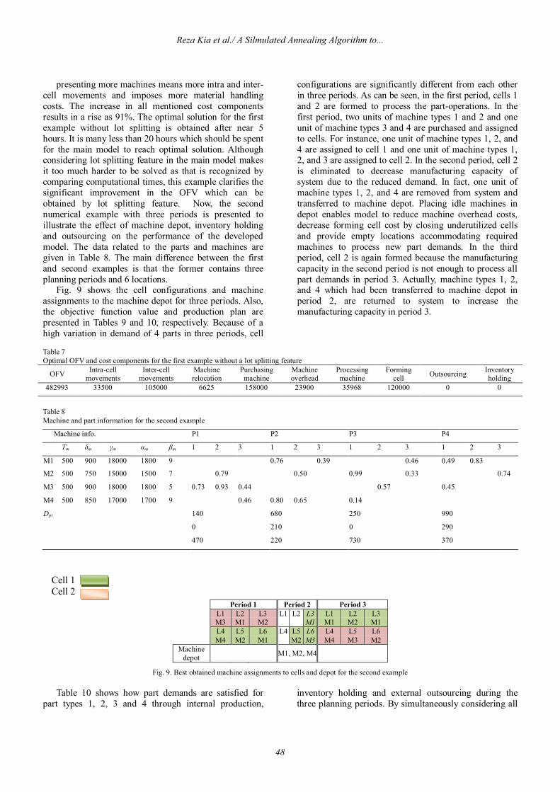
presenting more machines means more intra and inter-cell movements and imposes more material handling costs. The increase in all mentioned cost components results in a rise as 91%. The optimal solution for the first example without lot splitting is obtained after near 5 hours. It is many less than 20 hours which should be spent for the main model to reach optimal solution. Although considering lot splitting feature in the main model makes it too much harder to be solved as that is recognized by comparing computational times, this example clarifies the significant improvement in the OFV which can be obtained by lot splitting feature. Now, the second numerical example with three periods is presented to illustrate the effect of machine depot, inventory holding and outsourcing on the performance of the developed model. The data related to the parts and machines are given in Table 8. The main difference between the first and second examples is that the former contains three planning periods and 6 locations.

Fig. 9 shows the cell configurations and machine assignments to the machine depot for three periods. Also, the objective function value and production plan are presented in Tables 9 and 10, respectively. Because of a high variation in demand of 4 parts in three periods, cell

configurations are significantly different from each other in three periods. As can be seen, in the first period, cells 1 and 2 are formed to process the part-operations. In the first period, two units of machine types 1 and 2 and one unit of machine types 3 and 4 are purchased and assigned to cells. For instance, one unit of machine types 1, 2, and 4 are assigned to cell 1 and one unit of machine types 1, 2, and 3 are assigned to cell 2. In the second period, cell 2 is eliminated to decrease manufacturing capacity of system due to the reduced demand. In fact, one unit of machine types 1, 2, and 4 are removed from system and transferred to machine depot. Placing idle machines in depot enables model to reduce machine overhead costs, decrease forming cell cost by closing underutilized cells and provide empty locations accommodating required machines to process new part demands. In the third period, cell 2 is again formed because the manufacturing capacity in the second period is not enough to process all part demands in period 3. Actually, machine types 1, 2, and 4 which had been transferred to machine depot in period 2, are returned to system to increase the manufacturing capacity in period 3.

Table 7 Optimal OFV and cost components for the first example without a lot splitting feature

Inventory holding Outsourcing Forming

cell Processing machine

Machine overhead

Purchasing machine

Machine relocation


Intra-cell movements OFV

0 0 120000 35968 23900 158000 6625 105000 33500 482993

Table 8 Machine and part information for the second example

P4 P3 P2 P1 Machine info.

3 2 1 3 2 1 3 2 1 3 2 1 βm αm γm δm Tm

0.83 0.49 0.46 0.39 0.76 9 1800 18000 900 500 M1

0.74 0.33 0.99 0.50 0.79 7 1500 15000 750 500 M2

0.45 0.57 0.44 0.93 0.73 5 1800 18000 900 500 M3

0.14 0.65 0.80 0.46 9 1700 17000 850 500 M4

990 250 680 140 Dpt

290 0 210 0

370 730 220 470

Period 1 Period 2 Period 3

L1 M3

L2 M1

L3 M2 L1

L2

L3 M1

L1 M1

L2 M2

L3 M1

L4 M4

L5 M2

L6 M1 L4

L5 M2

L6 M3

L4 M4

L5 M3

L6 M2

Machine depot M1, M2, M4

Fig. 9. Best obtained machine assignments to cells and depot for the second example Table 10 shows how part demands are satisfied for

part types 1, 2, 3 and 4 through internal production, inventory holding and external outsourcing during the three planning periods. By simultaneously considering all

Cell 1 Cell 2


48

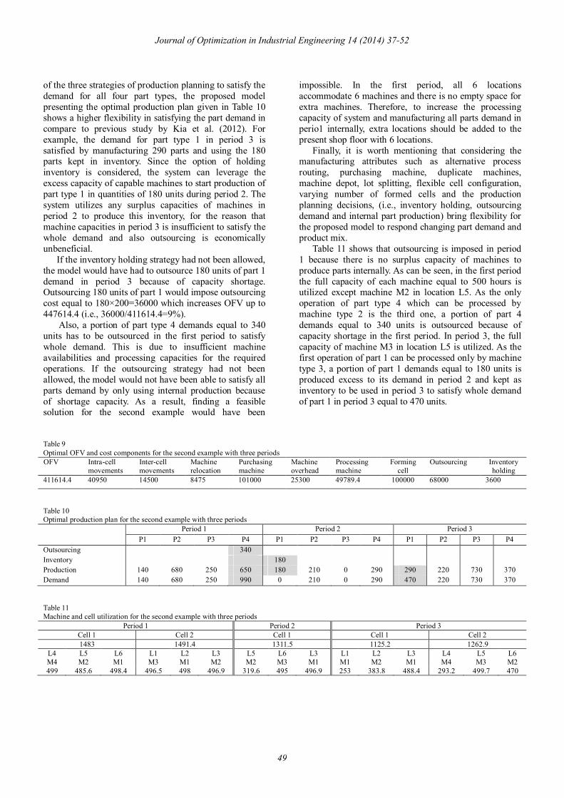
of the three strategies of production planning to satisfy the demand for all four part types, the proposed model presenting the optimal production plan given in Table 10 shows a higher flexibility in satisfying the part demand in compare to previous study by Kia et al. (2012). For example, the demand for part type 1 in period 3 is satisfied by manufacturing 290 parts and using the 180 parts kept in inventory. Since the option of holding inventory is considered, the system can leverage the excess capacity of capable machines to start production of part type 1 in quantities of 180 units during period 2. The system utilizes any surplus capacities of machines in period 2 to produce this inventory, for the reason that machine capacities in period 3 is insufficient to satisfy the whole demand and also outsourcing is economically unbeneficial.

If the inventory holding strategy had not been allowed, the model would have had to outsource 180 units of part 1 demand in period 3 because of capacity shortage. Outsourcing 180 units of part 1 would impose outsourcing cost equal to 180×200=36000 which increases OFV up to 447614.4 (i.e., 36000/411614.4=9%).

Also, a portion of part type 4 demands equal to 340 units has to be outsourced in the first period to satisfy whole demand. This is due to insufficient machine availabilities and processing capacities for the required operations. If the outsourcing strategy had not been allowed, the model would not have been able to satisfy all parts demand by only using internal production because of shortage capacity. As a result, finding a feasible solution for the second example would have been

impossible. In the first period, all 6 locations accommodate 6 machines and there is no empty space for extra machines. Therefore, to increase the processing capacity of system and manufacturing all parts demand in perio1 internally, extra locations should be added to the present shop floor with 6 locations.

Finally, it is worth mentioning that considering the manufacturing attributes such as alternative process routing, purchasing machine, duplicate machines, machine depot, lot splitting, flexible cell configuration, varying number of formed cells and the production planning decisions, (i.e., inventory holding, outsourcing demand and internal part production) bring flexibility for the proposed model to respond changing part demand and product mix.

Table 11 shows that outsourcing is imposed in period 1 because there is no surplus capacity of machines to produce parts internally. As can be seen, in the first period the full capacity of each machine equal to 500 hours is utilized except machine M2 in location L5. As the only operation of part type 4 which can be processed by machine type 2 is the third one, a portion of part 4 demands equal to 340 units is outsourced because of capacity shortage in the first period. In period 3, the full capacity of machine M3 in location L5 is utilized. As the first operation of part 1 can be processed only by machine type 3, a portion of part 1 demands equal to 180 units is produced excess to its demand in period 2 and kept as inventory to be used in period 3 to satisfy whole demand of part 1 in period 3 equal to 470 units.

Table 9 Optimal OFV and cost components for the second example with three periods

Inventory holding

Outsourcing Forming cell

Processing machine

Machine overhead

Purchasing machine

Machine relocation


Intra-cell movements

OFV

3600 68000 100000 49789.4 25300 101000 8475 14500 40950 411614.4

Table 10 Optimal production plan for the second example with three periods

Period 1 Period 2 Period 3 P1 P2 P3 P4 P1 P2 P3 P4 P1 P2 P3 P4

Outsourcing 340 Inventory 180 Production 140 680 250 650 180 210 0 290 290 220 730 370 Demand 140 680 250 990 0 210 0 290 470 220 730 370

Table 11 Machine and cell utilization for the second example with three periods

Period 1 Period 2 Period 3 Cell 1 Cell 2 Cell 1 Cell 1 Cell 2 1483 1491.4 1311.5 1125.2 1262.9

L4 L5 L6 L1 L2 L3 L5 L6 L3 L1 L2 L3 L4 L5 L6 M4 M2 M1 M3 M1 M2 M2 M3 M1 M1 M2 M1 M4 M3 M2 499 485.6 498.4 496.5 498 496.9 319.6 495 496.9 253 383.8 488.4 293.2 499.7 470


49

In this model, some of the PP attributes such as inventories holding and outsourcing of parts are incorporated to form the manufacturing cells because DCMS and PP decisions are interrelated and may not be handled sequentially (Defersha and Chen, 2007). In fact, a trade-off between outsourcing costs, holding costs and internal production costs (i.e., forming cells, material handling, machine purchase, machine overhead, machine relocation and machine processing) is managed.

In this section, twelve example problems are solved using the extended SA to evaluate its computational

efficiency in terms of objective value and computation time. The obtained solutions by SA are compared with those obtained by GAMS software and shown in Table 12.

As it has been reported in the literature, an effective cooling schedule is essential for reducing the amount of time required by the algorithm to find an optimal solution. But cooling schedules are almost always heuristic and it would be needed to balance moderately the computational time with the simulated annealing dependence on problem size.

Table 12 Comparison between SA and GAMS

Relative gap (٪)

Time (secons)

OFV

SA parameters

Problem size

GAMS SA

GAMS SA

Coo

ling

rate

MC

L

Fina

l tem

pera

ture

Initi

al te

mpe

ratu

re

N

umbe

r of l

ocat

ions

Num

ber o

f ope

ratio

ns p

er p

art

Num

ber o

f cel

ls Num

ber o

f mac

hine

s

Num

ber o

f per

iods

Num

ber o

f par

ts

Exam

ple

num

ber

0 0.19 11

122395 opt 122395.5

0.995 30 100 3000

4 2 2 2 2 2 1

0 25 13

174926 opt 174926

0.995 30 100 3000

5 3 2 3 2 2 2

4 4773 562

243124 opt 254300

0.995 50 100 50000

6 3 2 4 2 3 3

1 4472 955

276286 opt 280296

0.995 50 100 50000

7 3 3 4 2 4 4

3 7400 1003

264821 Best 274911

0.995 200 100 100000

8 3 3 5 2 4 5

-2 10147 659

321303Best 314022

0.995 200 100 100000

8 3 3 5 2 5 6

-4 13012 1318 412762

Best 394624

0.995 200 100 100000

8 3 2 5 3 5 7

-1 34608 883

312602.Best 309281

0.995 200 100 150000

6 4 2 5 3 5 8

5 21162 578

333556.Best 351090

0.995 200 100 150000

6 3 2 5 4 6 9

0 14658 278

208639.Best 208050

0.995 200 100 150000

6 3 2 4 4 4 10

-3 15026 3518

494261.Best 480924

0.995 200 100 200000

9 4 3 4 3 4 11

- - 3013 Out of

Memory 482320

0.995 200 100 200000

10 3 3 6 4 6 12

By carrying out several experiments on small

numerical samples 1-4 to gain insights into some assumptions and intuition behind cooling schedules, a theoretical framework for parameter setting of the simulated annealing algorithm is presented based on the model size. The simulated annealing schedule is defined

by initial temperatures in points [30000, 50000, 100000, 150000], a MCL in points [30, 50, 200] and final temperatures set to 100 as well as a cooling rate α equal to 0.995.

Because of exponential reduction of error probability, several short-term runs of SA results better than a long-


50

term one (Defersha and Chen, 2008). Hence, each run has been repeated 5 times to solve each example and the best obtained solution among them has been reported.

Since there are numerous decision variables and constraints in the proposed model, some of the numerical examples cannot be solved in a reasonable time by GAMS. Therefore, the solving process will be continued until the GAMS software encounters a resource limit as an out of memory message. At this point, the best obtained value of objective function is reported as GAMSBest to be compared with SA.

GAMS can only reach optimal solutions for examples 1-4, reported as GAMSOpt. For the examples 5-11, GAMS is interrupted because of out of memory predicament. As a result, the best obtained solutions for those examples are not optimal. Generating numerical examples is stopped at example 12, as the solution space is enlarged so much that GAMS even cannot generate a feasible solution before encountering out of memory message. As can be seen, the obtained solutions by SA are better than those obtained by GAMS for examples 6-8 and 10-11. This can be regarded as a remarkable achievement for a metaheuristic algorithm, especially in solving large-scaled problems which cannot be solved optimally by optimization packages such as GAMS. In general, the following results can be concluded: SA algorithm found the optimal solutions, in

nearly as same computational times as GAMS for example problems 1 and 2. In addition, for examples 3-5 and 9, the near optimal solutions are obtained by SA in a relative gap lower than 5% compared to those obtained by GAMS in less computational times.

The SA algorithm found better near-optimal solutions than GAMS in less computational times for example problems 6-8 and 10-11.

These promising results were obtained by SA because of the elaborately-designed solution representation schema, hierarchical procedure to generate initial solution and explorative solution mutation operators built into the SA algorithm.

5. Conclusion

This paper presented a mixed-integer linearized programming (MINLP) model integrating CF, GL and PP decisions under a dynamic environment. The presented model has combined large portion of design features introduced in the previous studies, such as alternative process routings, operation sequence, processing time, production volume of parts, purchasing machine, duplicate machines, machine capacity, lot splitting, group layout, multi-rows layout of equal area facilities, and flexible reconfiguration. Additionally, it has addressed other important design features including machine depot, variable number of cells, outsourcing and inventory holding of parts. The effect of newly-incorporated design

features on improving the performance of developed model has been illustrated by the numerical examples. The obtained results revealed that the variable number of cells could considerably improve the performance of extended model by reducing forming cell cost. Furthermore, machine depot could be effective in improving the performance of model by reducing machine overhead cost and configuring cells more usefully due to removing idle machines from cells. As well, production planning decisions were shown that could be improving by satisfying high volume demands due to leveling machine utilization in different periods.

The extended model was capable to determine optimally the production volume of alternative processing routes of each part, the material flow happening between different machines, the cell configuration, the machine locations, the number of formed cells, the number of purchased machines, the number of machines kept in depot, the production plan for each part type by satisfying demand through internal production, outsourcing and inventory holding. The objective was minimizing the total costs of intra and inter-cell material handling, machine relocation, purchasing new machines, machine overhead, machine processing, forming cells, outsourcing and inventory holding.

Since the integrated model belongs to NP-hard problems, an efficient simulated annealing algorithm with an effective solution structure and seven mutation operators has been developed to solve the model. In this study, a heuristic hierarchical procedure was designed to generate the initial solution with good quality. In addition, the solution structure was presented as a matrix with seven ingredients fulfilled hierarchically to satisfy all constraints and successive solutions were produced from the initial solution by implementing elaborately-designed mutation operators. All components in the objective functions could be influenced by the designed operators to more exploration of solution space. The performance of SA was evaluated and compared to GAMS software by 12 small/medium-sized problems taken from the literature, with respect to the OFV and computational time. In these tests, the proposed SA algorithm found the better solutions and performed better than the GAMS especially as the size of problem increases.

Incorporating other features, such as introducing uncertainty in part demands, machine time capacity and cost coefficients, integrating with reliability and labor issues, designing layout of unequal-area facilities, and solving more numerical examples especially in real cases using other new meta-heuristics will be left to future research.

References

[1] Ahkioon, S. Bulgak, A.A. and Bektas, T. (2009). ‘Cellular manufacturing systems design with routing flexibility, machine procurement, production planning and dynamic


51

system reconfiguration’, International Journal of Production Research, 47(6), 1573–1600.

[2] Baykasoglu, A. and Gindy, N.N.Z. (2001). ‘A simulated annealing algorithm for dynamic layout problem’, Computers & Operations Research, 28(14), 1403–1426.

[3] Defersha, F.M. and Chen, M. (2006). ‘A comprehensive mathematical model for the design of cellular manufacturing systems’, International Journal of Production Economics, 103, 767–783.

[4] Defersha, F.M. and Chen, M. (2007). ‘A parallel genetic algorithm for dynamic cell formation in cellular manufacturing systems’, International Journal of Production Research, 45 (1), 1–25.

[5] Defersha, F.M. and Chen, M. (2008). ‘A parallel multiple Markov chain simulated annealing for multi-period manufacturing cell formation problems’, International Journal of Advance Manufacturing Technology, 37, 140–56.

[6] Defersha, F.M. and Chen, M. (2009). ‘Simulated annealing algorithm for dynamic system reconfiguration and production planning in cellular manufacturing’, Int. J. Manufacturing Technology and Management, 17(1/2), 103–124.

[7] Drolet, J. Marcoux, Y, and Abdulnour, G. (2008). ‘Simulation-based performance comparison between dynamic cells, classical cells and job shops: a case study’, International Journal of Production Research, 46(2), 509–536.

[8] Javadi, B. Jolai, F. Slomp, J. Rabbani, M. and Tavakkoli-Moghaddam, R. (2013). ‘An integrated approach for the cell formation and layout design in cellular manufacturing systems’, International Journal of Production Research, DOI:10.1080/00207543.2013.791755.

[9] Jolai, F. Tavakkoli-Moghaddam, R. Golmohammadi, A. and Javadi, B. (2011). ‘An Electromagnetism-like algorithm for cell formation and layout problem’, Expert Systems with Applications, 39(2), 2172-2182.

[10] Kia, R. Shirazi, H. Javadian, N. and Tavakkoli-Moghaddam, R. (2013). ‘A multi-objective model for designing a group layout of a dynamic cellular manufacturing system’, Journal of Industrial Engineering International, 9:8.

[11] Kia, R. Baboli, A. Javadian, N. Tavakkoli-Moghaddam, R. Kazemi, M. and Khorrami, J. (2012). ‘Solving a group layout design model of a dynamic cellular manufacturing system with alternative process routings, lot splitting and flexible reconfiguration by simulated annealing’, Computers & Operations Research, 39, 2642–2658.

[12] Kamali-Dolat-Abadi, A.H. Pasandideh, S.H.R. and Abdi-Khalife, M. (2010) ‘Layout of cellular manufacturing system in dynamic condition’, Journal of Industrial Engineering. 3(5), 43-54.

[13] Kirkpatrick, S. Gelatt, Jr.C.D. and Vecchi, MP. (1983). ‘Optimisation by simulated annealing’, Science, 220(6), 71-80.

[14] Majazi Dalfard, V. (2013). ‘New mathematical model for problem of dynamic cell formation based on number and average length of intra and intercellular movements’, Applied Mathematical Modelling, 37 (4), 1884-1896.

[15] Mahdavi, I. Aalaei, A. Paydar, M.M. and Solimanpur, M. (2010). ‘Designing a mathematical model for dynamic cellular manufacturing systems considering production planning and worker assignment’, Computers and Mathematics with Applications. 60, 1014–25.

[16] Mungwattana, A. (2000). ‘Design of cellular

manufacturing systems for dynamic and uncertain production requirements with presence of routing flexibility, PhD thesis submitted to the Faculty of the Virginia Polytechnic Institute and State University, Blackburg, VA.

[17] Rafiee, K. Rabbani, M. Rafiei, H. and Rahimi-Vahed, A. (2011). ‘A new approach towards integrated cell formation and inventory lot sizing in an unreliable cellular manufacturing system’, Applied Mathematical Modelling, 35, 1810–1819.

[18] Rheault, M. Drolet, J. and Abdulnour, G. (1995). ‘Physically reconfigurable virtual cells: a dynamic model for a highly dynamic environment’, Computers & Industrial Engineering, 29 (1–4). 221–225.

[19] Rosenblatt, M.J., (1986). ‘The dynamics of plant layout’, Management Science, 32 (1), 76–86.

[20] Saidi-Mehrabad, M. and Mirnezami-Ziabari, S. M. (2011). ‘Developing a Multi-objective Mathematical Model for Dynamic Cellular Manufacturing Systems’, Journal of Optimization in Industrial Engineering. 4(7), 1-9

[21] Safaei, N. and Tavakkoli-Moghaddam, R. (2009). ‘Integrated multi-period cell formation and subcontracting production planning in dynamic cellular manufacturing’, International Journal of Production Economics, 120 (2), 301–314.

[22] Safaei, N. Saidi-Mehrabad, M. and Jabal-Ameli, M.S. (2008). ‘A hybrid simulated annealing for solving an extended model of dynamic cellular manufacturing system’, European Journal of Operational Research. 185. 563–592.

[23] Saidi-Mehrabad, M. and Safaei, N. (2007). ‘A new model of dynamic cell formation by a neural approach’, International Journal of Advanced Manufacturing Technology. 33, 1001–1009.

[24] Saxena, L.K. and Jain, P.K. (2011). ‘Dynamic cellular manufacturing systems design—a comprehensive model’, International Journal of Advanced Manufacturing Technology 53 (1), 11–34.

[25] Tavakkoli-Moghaddam, R. Safaei, N. and Sassani, F. (2008). ‘A new solution for a dynamic cell formation problem with alternative routing and machine costs using simulated annealing’, Journal of Operational Research Society, 59(4): 443–54.

[26] Venugopal, V. And Narendran, T. (1992). ‘Cell formation in manufacturing systems through simulated annealing: An experimental evaluation’, European Journal of Operational Research. 63, 409–22.

[27] Wu, X. Chu, C.H. Wang, Y. and Yan, W. (2007). ‘A genetic algorithm for cellular manufacturing design and layout’, European Journal of Operational Research. 181, 156–167.

[28] Wemmerlov, U. Hyer, and N.L. (1986). ‘Procedures for the part family/machine group identification problem in cellular manufacture’, Journal of Operations Management. 6, 125–147.


52

a simulated annealing algorithm to determine a group

Documents