June 2001

NASA/CR-2001-210874

A Small Aircraft Transportation System(SATS) Demand Model

Dou Long, David Lee, Jesse Johnson, and Peter KostiukLogistics Management Institute, McLean, Virginia

The NASA STI Program Office ... in Profile

Since its founding, NASA has been dedicatedto the advancement of aeronautics and spacescience. The NASA Scientific and TechnicalInformation (STI) Program Office plays a keypart in helping NASA maintain this importantrole.

The NASA STI Program Office is operated byLangley Research Center, the lead center forNASA’s scientific and technical information.The NASA STI Program Office providesaccess to the NASA STI Database, the largestcollection of aeronautical and space scienceSTI in the world. The Program Office is alsoNASA’s institutional mechanism fordisseminating the results of its research anddevelopment activities. These results arepublished by NASA in the NASA STI ReportSeries, which includes the following reporttypes:

• TECHNICAL PUBLICATION. Reportsof completed research or a majorsignificant phase of research thatpresent the results of NASA programsand include extensive data or theoreticalanalysis. Includes compilations ofsignificant scientific and technical dataand information deemed to be ofcontinuing reference value. NASAcounterpart of peer-reviewed formalprofessional papers, but having lessstringent limitations on manuscriptlength and extent of graphicpresentations.

• TECHNICAL MEMORANDUM.Scientific and technical findings that arepreliminary or of specialized interest,e.g., quick release reports, workingpapers, and bibliographies that containminimal annotation. Does not containextensive analysis.

• CONTRACTOR REPORT. Scientific andtechnical findings by NASA-sponsoredcontractors and grantees.

• CONFERENCE PUBLICATION.Collected papers from scientific andtechnical conferences, symposia,seminars, or other meetings sponsoredor co-sponsored by NASA.

• SPECIAL PUBLICATION. Scientific,technical, or historical information fromNASA programs, projects, and missions,often concerned with subjects havingsubstantial public interest.

• TECHNICAL TRANSLATION. English-language translations of foreignscientific and technical materialpertinent to NASA’s mission.

Specialized services that complement theSTI Program Office’s diverse offeringsinclude creating custom thesauri, buildingcustomized databases, organizing andpublishing research results ... evenproviding videos.

For more information about the NASA STIProgram Office, see the following:

• Access the NASA STI Program HomePage at http://www.sti.nasa.gov

• E-mail your question via the Internet tohelp@sti.nasa.gov

• Fax your question to the NASA STIHelp Desk at (301) 621-0134

• Phone the NASA STI Help Desk at (301)621-0390

• Write to:NASA STI Help DeskNASA Center for AeroSpace Information7121 Standard DriveHanover, MD 21076-1320

National Aeronautics andSpace Administration

Langley Research Center Prepared for Langley Research CenterHampton, Virginia 23681-2199 under Contract NAS2-14361

June 2001

NASA/CR-2001-210874

A Small Aircraft Transportation System(SATS) Demand Model

Dou Long, David Lee, Jesse Johnson, and Peter KostiukLogistics Management Institute, McLean, Virginia

Available from:

NASA Center for AeroSpace Information (CASI) National Technical Information Service (NTIS)7121 Standard Drive 5285 Port Royal RoadHanover, MD 21076-1320 Springfield, VA 22161-2171(301) 621-0390 (703) 605-6000

iii

LOGISTICS MANAGEMENT INSTITUTE

A Small Aircraft Transportation System (SATS)Demand Model

NS004S1

Executive Summary

The Small Aircraft Transportation System (SATS) is envisioned to take advantageof technology advances in aircraft engines, avionics, airframes, navigation equip-ment, communications, and pilot training to make it the new generation of generalaviation (GA) that will let people travel from small airports. SATS not only willhelp to break the gridlock at large commercial airports by diverting traffic to non-hub small airports, it also can generate new air traffic demand as it can reduce thedoor-to-door time for travels from or to a place close to a small airport. With highspeed aircraft, numerous airports, an affordable cost, and easy pilot training,SATS can provide better door-to-door travel time, enhance mobility, and stimu-late business activity.

This report explains our SATS demand modeling at the national, airport, and air-space levels. We constructed a series of models following the general systemsengineering principle of top-down and modular approach. Our three principalmodels are the SATS Airport Demand Model (SATS-ADM), SATS Flight De-mand Model (SATS-FDM), and LMINET-SATS. SATS-ADM models SATS op-erations, by aircraft type, from the forecasts in fleet, configuration andperformance, utilization, and traffic mixture. Given the SATS airport operationssuch as the ones generated by SATS-ADM, SATS-FDM constructs the SATS ori-gin and destination (O&D) traffic flow based on the solution of the gravity model,from which it then generates SATS flights using the Monte Carlo simulationbased on the departure time-of-day profile. LMINET-SATS, an extension ofLMINET, models SATS demands at airspace and airport by all aircraft operationsin the United States.

The models presented in this report can be the powerful tools to policy decisionmakers in air traffic system planning, especially in SATS. The models will helpproject SATS demands for airports and airspace. The models are built with suffi-cient parameters to give users flexibility and ease of use to analyze SATS demandunder different scenarios. Several case studies are included to illustrate the use ofthe models, which also are helpful in designing the new air traffic managementsystem to cope with SATS traffic.

iv

The figures we present in this study are not forecasts; they are the results of what-if studies. The models, albeit developed with empirical data fitting and flexibilityto change the parameters, are not forecast models themselves. The models, how-ever, are constructed so they can easily hook to the SATS Economic DemandModel (SATS-EDM), which will generate SATS demand forecast from the air-craft performance data and the socioeconomic data about areas surrounding theairports. With SATS-EDM in our model suite, we will have a complete SATSdemand forecast model. In the last chapter we include our preliminary thoughtson how to construct SATS-EDM.

v

Contents

Chapter 1 Modeling Framework .......................................................................1-1

Chapter 2 SATS Airport Demand Model..........................................................2-1

SELECTED AIRPORTS IN THE STUDY ..................................................................................2-1

GA AIRPORT DEMOGRAPHIC AND ECONOMIC DATABASE .................................................2-4

AN ECONOMIC DEMAND MODEL OF AIRPORT GA OPERATION.........................................2-6

DEFAULT AIRPORT GA OPERATION MODEL......................................................................2-9

GA TRAFFIC MEASURES AND THEIR USE IN SATS DEMAND FORECAST........................2-12

Chapter 3 SATS Flight Demand Model ............................................................3-1

THE GRAVITY MODEL OF ORIGIN AND DESTINATION DEMAND ........................................3-2

GA FLIGHT PROFILE.........................................................................................................3-3

Distance Distributions................................................................................................3-3

Time-of-day Profile....................................................................................................3-8

MONTE CARLO SIMULATION OF GA FLIGHT DEMAND ...................................................3-10

Chapter 4 LMINET-SATS ................................................................................4-1

AIRSPACE FOR PISTON-DRIVEN SATS AIRPLANES............................................................4-1

Airlines.......................................................................................................................4-1

Special Use Airspace..................................................................................................4-3

Mountains...................................................................................................................4-4

SATS AND ATM STAFFING..............................................................................................4-4

DEFINITION AND OPERATION OF LMINET-SATS ............................................................4-6

Considerations for Adding a SATS Underlayer to LMINET ....................................4-7

SATS airports...........................................................................................................4-12

LMINET-SATS Operations .....................................................................................4-13

RESULTS..........................................................................................................................4-14

An initial exercise.....................................................................................................4-14

Effects of Improved Strategies.................................................................................4-20

Conclusions ..............................................................................................................4-23

vi

Chapter 5 Summary and Future Work ..............................................................5-1

References

Appendix A Parameter Estimation of the Gravity Model

FIGURES

Figure 1-1. Top-down, Modular SATS Demand Modeling...................................................1-3

Figure 2-1. Lorenz Curve of GA Operations .........................................................................2-3

Figure 2-3. Airport Operations Model Schematic................................................................2-12

Figure 3-1. Distance Distribution of Single–Engine Aircraft ................................................3-4

Figure 3-2. Distance Distribution of Multi-Engine Aircraft ..................................................3-5

Figure 3-3. Distance Distribution of Jet-Engine Aircraft.......................................................3-5

Figure 3-4. Monthly GA Flights ..........................................................................................3-10

Figure 4-1. Fuel Burn and Associated Airspeed For Canadair CL600 Regional Jet ............4-2

Figure 4-2. Fuel Burn and Associated Airspeed ....................................................................4-2

Figure 4-3. Variation of Fuel Burn with TAS at FL 180, Embraer E120 ..............................4-3

Figure 4-4. Distribution of Distances of 889 IFR Flights of Light Aircraft...........................4-6

Figure 4-5. Thirty nm Zones around LMINET Airports........................................................4-7

Figure 4-6. Low-Altitude Sectors for Albuquerque Air Route Traffic Control Center .........4-7

Figure 4-7. Geographic Enroute Sectors ................................................................................4-8

Figure 4-8. Enroute Sector Structure For Light-Aircraft SATS Operations ..........................4-9

Figure 4-9. FAA High-Altitude Sectors.................................................................................4-9

Figure 4-10. Example Trajectory .........................................................................................4-10

Figure 4-11. SATS Airports .................................................................................................4-13

Figure 4-12. Hourly SATS Departures Required to Meet 1 Percent of RPM Demand .......4-15

Figure 4-13. Piston ILS Arrivals at Van Nuys, California...................................................4-15

Figure 4-14. Piston ILS Arrivals at Morristown, New Jersey..............................................4-16

Figure 4-15. Hourly Demand For Busy Sectors, 2007.........................................................4-18

Figure 4-16. SATS TRACON Demands, 2007....................................................................4-18

Figure 4-17. Hourly Demand For Busy Sectors, 2022.........................................................4-19

Figure 4-18. SATS TRACON Demands, 2022....................................................................4-19

Figure 4-19. Hourly Piston-SATS Arrivals to SATS Airports Near EWR..........................4-20

Contents

vii

Figure 4-20. SATS Operations to Supply RPM Deficit.......................................................4-21

Figure 4-21. Piston-SATS Arrivals to VNY, Deficit Case ..................................................4-21

Figure 4-22. Arrivals to Sector 205......................................................................................4-22

Figure 4-23. Arrivals To SATS Airports Near EWR, Deficit Case.....................................4-22

TABLES

Table 2-1. Airport Activity Distribution ................................................................................2-2

Table 2-2. Top 10 GA Operations Airports ...........................................................................2-3

Table 2-3. Airport Demographic and Economic Database ....................................................2-5

Table 2-4. Total Itinerant Landings by Category and Region..............................................2-10

Table 2-5. Number of Aircraft by Category and Region .....................................................2-11

Table 2-6. Aircraft Utilization Rate by Category and Region .............................................2-11

Table 2-8. Actual Use GA and AT Hours Flown in 1998....................................................2-14

Table 2-9. Total TPM by Engine Type and Traffic Distribution in 1998............................2-14

Table 2-10. Percentage of Total Operations Flown by Aircraft Type in 1998 ...................2-14

Table 2-11. Constrained and Unconstrained RPM (Billion) Forecasts................................2-15

Table 2-12. Additional SATS Operations for 1 Percent of Commercial RPM....................2-15

Table 2-13. Additional SATS Operations to Fill the Gap of Unsatisfied CommercialTraffic.............................................................................................................................2-15

Table 3-1. Percentiles of Average Daily GA Operations at TAF Airports ............................3-1

Table 3-2. Samples of ETMS Data in the Distance Distribution Estimation.........................3-4

Table 3-3. Distance (nmi) Statistics for Combined Data Sets................................................3-6

Table 3-4. Model Parameters for Weibull Distribution .........................................................3-6

Table 3-5. Estimated Distance (nmi) Statistics Using a Weibull Distribution......................3-6

Table 3-6. Time-of-day Probability Distribution Function Used in the Simulation ..............3-9

1-1

Chapter 1 Modeling Framework

The transportation system is a vital part of a dynamic economy. For centuries,cities and economies have developed at seaports and along riverbanks, at the rail-road and interstate highway intersections, and more recently near airports. Sincethe first flight made by the Wright brothers about a century ago, the air transpor-tation industry has matured. It has developed from a means of delivering mail to ameans of travel for the rich to today’s necessary means of travel for conductingbusiness and pursuing leisure. In the United States alone in 2000, there were morethan 670 million enplanements and more than 670 billion RPMs. Commercial airtransport service has become so important to our business activity and our livesthat any disturbance in its service by inclement weather or inadequate air trafficcapacity is met by public outcry.

Because of the imbalance of increasing air traffic demand and the relatively con-stant air traffic capacity, air traffic congestion will become worse. Studies haveconcluded that our National Airspace System (NAS) will reach gridlock in abouta decade, precluding reliable commercial air transport unless demand is curtailed.The more realistic prediction is that airlines will raise ticket prices to curb demandfrom marginal travelers and curtail operations to remain within the air traffic ca-pacity. These measures will be at the expense of national business activity and thegeneral consumer welfare.

Because travel demand is positively related to population and per capita income,our air travel demand will increase with growing population and economy [1, 2].Our propensity of air travel, in the meantime, will also be increasing. The BabyBoomer generation will retire with the money and time to travel. The value ofhuman time is increasingly valuable in the fast-paced information age. The econ-omy demands that goods are manufactured and delivered “just-in-time.”

Small Aircraft Transportation System (SATS) provides alternatives in airtravel—more frequent flights of small aircraft take off and land at small airports.The recent advances in engines, avionics, airframe, navigation, communication,and pilot training have made a new generation of general aviation (GA) possible.SATS will take advantage of the vast pool of small airports to break the gridlockof air traffic congestion.

Air traffic congestion is mostly airport induced, either from insufficient runways,taxiways, gates, or insufficient airspace capacity around airports [3]. The UnitedStates has more than 5,000 airports and about 12,000 landing strips, but onlyabout 200 airports have jet operations. SATS will help break the gridlock at largecommercial airports by diverting traffic to small airports. It also can pick up latent

1-2

air traffic demand because it can speed up door-to-door trip time. With highspeed, numerous available airports, affordable costs, and easy pilot training,SATS can provide better door-to-door travel time, enhance mobility, and stimu-late business activity.

This report explains SATS demand modeling. SATS is still in its formative stage,but many current generation GA aircraft such as the Cirrus-20 already have SATStechnical capabilities. Compared with current GA, SATS may

◆ change the speed of travel time and the reaches of destinations;

◆ alter avionics requirements for airport and airspace operations; and

◆ reduce operating costs and certification requirements.

Other factors will influence SATS operations. Pressurized cabins will enableSATS to fly at higher altitudes, requiring different air traffic control (ATC) serv-ice and different air traffic management (ATM) schemes. SATS can be treated asGA with different attributes, which our model will address. Our model will beflexible to account for retrofitting of current GA aircraft, modified attributes, ordifferent percentages of aircraft that have SATS attributes. With this flexibility,our SATS model is a GA model, and we will use SATS and GA interchangeablyin our modeling.

GA aircraft are classified1 as

◆ single-engine IFR,

◆ single-engine VFR,

◆ multi-engine VFR,

◆ multi-engine piston IFR,

◆ multi-engine turbo IFR, and

◆ jet.

Engine types determine the speed and reaches of an aircraft; avionics equipment(VFR/IFR) determine airport and ATC sector demands under different weatherconditions. Jets always are assumed to be IFR because flight altitude requires IFRflights.

1 Helicopter operations are not included in this report’s demand modeling because (1) airports

are not required for take off and landing and (2) most helicopter operations are VFR, and thus re-sult in few recorded flight tracks. We can capture only a few IFR helicopter flights a day in ourETMS data source.

Modeling Framework

1-3

Figure 1-1. Top-down, Modular SATS Demand Modeling

SATS-ADM SATS-FDM LMINET-SATS

Input:

socioeconomic data

scenario definition

Output:

operations at each airport by a/ctype

Component model:

SATS a/c utilization model

Input:

operations at each airport

time-of-day distribution

distance distribution

Output:

SATS schedule

Component model:

gravity distribution model

Monte Carlo simulation

Input:

air carrier and SATS schedule

SATS a/c & airport performance

Output:

demand & delays at sectors &TRCONs

delays at 2,865 airports

Component model:

LMINET

SATS a/c trajectory model

SATS airport capacity/delay model

Figure 1-1 shows our SATS demand model built in a top-down, modular fashionfollowing the general system engineering principle. There are three major compo-nent models with the following functionalities:

◆ SATS Airport Demand Model (SATS-ADM)

➤ Input—demographic and economic data, airport and aircraft perform-ance data;

➤ Output—annual number of operations by airport and aircraft type;

◆ SATS Flight Demand Model (SATS-FDM)

➤ Input—output of SATS-ADM;

➤ Output—GA flight schedule for entire GA airport network;

◆ LMINET-SATS

➤ Input—output of SATS-FDM

➤ Output—ATC-sector demand for the entire NAS.

From SATS-ADM to SATS-FDM to LMINET-SATS, the GA demand is moreand more detailed. The models are linked through input and output, which arecommon traffic measures used. Each model exists in its own right, and users cansubstitute them by using best-available information.

1-4

Chapters 2, 3, and 4 explain our three principal models, SATS-ADM, SATS-FDM, and LMINET-SATS. Each model has its own subcomponent models.Chapter 5 summarizes model capabilities and identifies future work. The appen-dixes list technical details of our model.

2-1

Chapter 2 SATS Airport Demand Model

SELECTED AIRPORTS IN THE STUDY

There are more than 5,000 airports and approximately 12,000 landing strips in theUnited States. The most comprehensive databases about these airports are theFAA’s Terminal Area Forecast (TAF) and the National Plan of Integrated AirportSystems (NPIAS). For each of the approximately 3,000 airports in the database,TAF maintains information about enplanements, operations, and based aircraft.Of the remaining 2,000 airports not included in the databases, about 1,000 are pri-vately owned but available for public use. Another 1,000 airports are publiclyowned but lack sufficient facilities, or do not have sufficient based aircraft, or arewithin 20 miles of a TAF airport [9].

In the NPIAS, airports (see Table 2-1) are classified as follows:

◆ Large hub—enplanement is more than 1 percent of the total U.S. enpla-nement;

◆ Medium hub—enplanement is more than 0.25 percent but less than 1 per-cent;

◆ Small hub—enplanement is more than 0.05 percent but less than 0.25 per-cent;

◆ Nonhub primary—enplanement is more than 10,000 but less than0.05 percent of the U.S. total;

◆ Other commercial—enplanement is more than 2,500 but less than 10,000annually; and

◆ Reliever—GA airports located close to major metropolitan areas.

2-2

Table 2-1. Airport Activity Distribution

Airport typeNumber of

airportsPercentage of all

enplanementsPercentage of active

GA aircraft

Airport typeNumber of air-

portsPercentage of all

enplanementsPercentage of active

GA aircraft

Large hub 29 67.3 1.3

Medium hub 42 22.2 3.8

Small hub 70 7.1 4.7

Nonhub primary 272 3.3 11.4

Other commercial 125 0.1 2.1

Reliever 334 0.0 31.5

Other GA 2,472 0.0 37.3

TAF Total 3,344 100.0 92.1

Source: NPIAS.

TAF airports cover 98 percent of the domestic U.S. population within 20 miles ofairport radii. The airports are distributed roughly one per county in rural areas andoften are located near the county seat. Of all TAF airports, 95 percent are consid-ered to have good or fair runway pavement. We selected the entire database ofTAF airports for our study because they cover almost the entire domesticU.S. population and serve current GA activity. Including additional airports doesnot offer sufficient benefits to justify the substantial effort required to collect ad-ditional airport data. With a selection of a smaller set of total TAF airports, it isstill possible for us to construct a sound model; however, it is not worth the addi-tional effort required to study out-of-network SATS traffic. If we select all TAFairports, we can ignore all out-of-network traffic as practically insignificant.

We have a network of 2,865 airports after excluding airports in Alaska, Hawaii,Puerto Rico, and Guam. If we rank those airports according to their itinerant GAoperations and plot them with the airport distribution, a Lorenz curve results, asshown in Figure 2-1 [5].

SATS Airport Demand Model

2-3

Figure 2-1. Lorenz Curve of GA Operations

0.0

0.1

0.2

0.3

0.4

0.5

0.6

0.7

0.8

0.9

1.0

0 500 1000 1500 2000 2500 3000

From this curve, we see that GA operations are concentrated. In fact, 100 airportsaccount for 25 percent of GA itinerant operation, 300 airports account for about50 percent, and 1,000 airports account for about 83 percent. Table 2-2 lists 10 air-ports with the most itinerant GA operations in 1997.

Table 2-2. Top 10 GA Operations Airports

Airport Itinerant GA Operations in 1997

VNY 373,781

SNA 156,216

DAB 232,059

LGB 221,046

APA 197,230

RVS 185,121

FTW 183,301

BFI 182,124

OAK 175,294

FXE 174,142

2-4

If we use 600 nmi radius as a criterion that an airport can reach by GA, then anairport in our SATS airport network can reach between 257 to 1,708 airports. Themedian number of airports that an airport can reach is 1,038. The range of the firstquartile and the third quartile is from 643 to 1,347. Any airport in the SATS net-work has a good number of other airports within its reach.

There is a slight negative correlation between the airport reach and the itinerantoperation. The Spearman correlation is -0.12514 [5]. We think this negative cor-relation is caused by some airports in California, which, because of their geo-graphic location, have limited number of airports among their reach but havelarge number of GA operations. Thus, we can say that the GA operation at oneairport generally does not depend on the number of airports among its reach, butmore on the characteristic of its reach.

GA AIRPORT DEMOGRAPHIC AND ECONOMIC

DATABASE

The GA Airport Demographic and Economic Database is used to extrapolate eco-nomic and demographic information from the current baseline year (1998) to thetwo future target years (2007 and 2022). A set of reference parameters can be cal-culated from the 1998 data. Projections are scaled from these reference parame-ters. For example, one set of parameters is scaled on total household income, thenprojected to total household income in the future target years.

The database starts with census track data mapped for 3,320 official FAA moni-tored U.S. airports. The FAA assigns each airport a unique three-letter airportidentifier.

The database also includes geographic information for region and state, and hubor reliever status. The important information regarding airport aviation status in-cludes enplanements, based aircraft, and operations.

The term, “enplanement” refers to one passenger boarding an aircraft; distanceflown and purpose are not relevant. There are five categories of enplanements: aircarrier, air taxi, commuter, U.S., and total. Because enplanement applies to com-mercial transportation only, numerous airports report zero enplanements across allcategories.

“Based aircraft” refers to the number of aircraft, by type, located at an airport.The aircraft types are single engine, multi-engine, jet engine, helicopter, other,and total based aircraft. Because commercial aircraft are never based in any air-port, the reported based aircraft are GA or air taxi only.

“Operation” is defined as either an aircraft takeoff or landing. Operations can beclassified by purpose. Operations can be itinerate (place to place) or local. Thetype of aircraft is military, general aviation, air taxi, or air carrier. Categories for

SATS Airport Demand Model

2-5

operations are air carrier itinerant, air taxi itinerate, general aviation itinerate,military itinerant, general aviation local, military local, and total operations.(There are no local air carrier or local air taxi operations).

Table 2-3. Airport Demographic and Economic Database

Description Variable Name

Location id Locid

Region Region

Airport Name Airport

City City

State State

Year Year

Hub Size Hub Size

Reliever Reliver

Air Carrier Approaches AirC App

Air Taxi Approaches AirT App

General Aviation Approaches GA App

Military Approaches Mil App

Total Approaches Tot App

Single Engine Based Aircraft SEB Air

Jet Engine Based Aircraft JEB Air

Multi Engine Based Aircraft MEB Air

Helicopter Based Aircraft HelB Air

Other Based Aircraft OthB Air

Total Based Aircraft TotB Air

Air Carrier Enplanements AC Enpla

Air Taxi Enplanements AT Enpla

Commuter Enplanements Co Enpla

US Flag Enplanements US Enpla

Foreign Flag Enplanements Fo Enpla

Total Enplanements To Enpla

Primary Air Carrier Overs Pr AC Ov

Primary Air Taxi Overs Pr AT Ov

Primary General Aviation Overs Pr GA Ov

Primary Military Overs Pr Mi Ov

Secondary Air Carrier Overs Se AC Ov

Secondary Air Taxi Overs Se AT Ov

Secondary General Aviation Overs Se GA Ov

Secondary Military Overs Se Mi Ov

Instrument Operations Total Overs InOps TO

Total Instrument Operations TotI Ops

Air Carrier Itinerant Operations ACIt Ops

Air Taxi Itinerant Operations ATIt Ops

General Aviation Itinerant Operations GAIt Ops

2-6

Table 2-3. Airport Demograhic and Economic Database(Continued)

Description Variable Name

Military Itinerant Operations MiIt Ops

General Aviation Local Operations GAL Ops

Military Local Operations MiL Ops

Total Operations Tot Ops

Population In All Rings Pop All

Population Ring 1 (Red) PopRing1

Population Ring 2 (Green) PopRing2

Population Ring 3 (Blue) PopRing3

Households In All Rings House All

Households Ring 1 (Red) HouseRg1

Households Ring 2 (Green) HouseRg2

Households Ring 3 (Blue) HouseRg3

Total Household Income In All Rings TtHsIn

Total Household Income Ring 1 (Red) TtHsIn1

Total Household Income Ring 2 (Green) TtHsIn2

Total Household Income Ring 3 (Blue) TtHsIn3

Average Household Income In All Rings AvHsInTT

Average Household Income Ring 1 (Red) AvHsInR1

Average Household Income Ring 2 (Green) AvHsInR2

Average Household Income Ring 3 (Blue) AvHsInR3

It is believed in NPIAS that 20 miles radius is a good measure surrounding an air-port because it corresponds about 30 minutes driving to the airport. The regionsurrounding an airport is divided into three rings in the database: the first ring iswithin 10 miles of the airport; the second ring is from 10 to 20 miles from the air-port; and the third ring is 20 to 50 miles from the airport. Some overlap existsbetween airports (i.e., a household may lie inside the rings of multiple airports).For each defined ring, the database contains population, number in a household,and total and average household income.

The following sections in this chapter discuss database use and its importance inour airport GA operation demand modeling.

AN ECONOMIC DEMAND MODEL OF AIRPORT GAOPERATION

In this section, we build a model of GA operations based on current observationsof socioeconomic variables. Current GA travel is not the SATS travel envisionedfor the future, although the current GA aircraft, especially corporate jets and thoseoperated in the timeshare program, certainly are SATS-capable. Our construction

SATS Airport Demand Model

2-7

of a current GA demand model can offer valuable insight into the SATS demandmodel.

Because the SATS forecast eventually must be at the airport level, the best datasource is our Airport Demographic and Economic Database. According toNPIAS, this data set covers about 98 percent of the total U.S. population, whichlives within 20-mile radii of the airports, or about 30 minutes of driving time to anairport.

The linear model is the simplest because the GA traffic is proportional to the sur-rounding population, although the proportions may be different for the three sur-rounding rings. For each airport, the following GA demand model is always true:

∑=

⋅=3

1iii PopRingGA α , [Eq. 2-1]

where GA is the measure of GA traffic to be specified, and α1, α2, α3 are the pa-rameters that measure the estimated propensity of the population to travel GA. Ifwe think the propensity for GA travel is linearly related to the average householdincome, i.e.,

,3,2,1, =⋅+= iAvHsInRiiii βδα [Eq. 2-2]

then the GA traffic can be rewritten as

)(3

1iii

iii AvHsInRPopRingPopRingGA ⋅⋅+⋅= ∑

=

βδ . [Eq. 2-3]

This is a linear model if we treat the products of PopRingi and AvHsInRi, i=1, 2,3, as separate variables. We think this model probably works only for the GA air-ports when the large, medium, and small hub airports are excluded, because hubairports are developed for commercial service. To further account for the some ofthe uniqueness GA airports have to attract travel demand, the GA operations mustbe related to commercial and air taxi traffic. Our GA demand model can be writ-ten as

.__)(3

1

OpsAtItEnplaAcAvHsInRPopRingPopRingGA iiii

ii ++⋅⋅+⋅= ∑=

βδ [Eq. 2-4]

If we use the itinerant GA operations as the measure of GA traffic in the abovelinear regression equation, then we can estimate the parameters. Based on 1998data, R2 is about 30 percent 1. This is not a terrible model, but it is not a terrificmodel either.

1 R2 is a goodness-of-fit of the model to the data, which measures as a percentage the vari-

ability of the observed data that can be explained by the model.

2-8

One cause of the lack of goodness-of-fit is the location of the airports. When werun the same model by region, where each of the nine regions has its own separateparameter estimates, then the R2s range from 30 percent through 60 percent. Thisis an improvement of the model, although the basic idea—that GA traffic is de-termined by population and average income—is unchanged.

When we run the model by state, the R2s range from 30 percent through 80 per-cent, with model improvement at the high end of R2 but not at the low end. Thismeans the airports are not homogenous enough at regional or state levels for GAtraffic at an airport to be explained by the surrounding population and its averageincome and location.

The general idea of this model is good, and model goodness of fit improves whenwe further classify airports geographically. With additional information about anairport’s equipage, access, weather statistics, and surroundings including incomedistribution and business activities, the model can be improved.

Additional information about an airport and its surroundings does not change ourbasic assumption that GA traffic is related to the surrounding population whosepropensity for GA activity is related directly to its income. Additional informationwill improve the GA demand model. With more information about the airport, wewill need to construct an airport-specific GA demand model (i.e., each airportdemand model will have its unique parameters.

Can we construct airport-specific GA demand models based on our GA AirportDemographic and Economic Database? The answer seems to be “no.” First, wehave only a few historical data points for 1980, 1990, and 1998 for each airport,which makes the estimation impossible. Even with more data points for each air-port, we cannot use all the data because of the structural change in the GA indus-try since enactment of the GA Revitalization Act in 1994.

Figure 2-2 shows historical and forecast traffic in the 3,320 airports in FAA’s1999 TAF. In the figure, ITN_AC, ITN_AT, ITN_GA, and LOC_GA, are the op-erations of air carrier, air taxi, itinerant GA, and local GA. The data from 1976through 1998 are based on observed counts; data beyond 1998 are forecasts. Re-versal of the GA traffic decline since enactment of the General Aviation Revitali-zation Act in 1994 clearly shows the structural change on GA traffic, whichreveals the dependence of GA traffic demand on the government policy. Fromthis we can further infer that the SATS demand will also depend on the govern-ment policy, or more broadly, on the general SATS operation environment. Thedifficulty to predict the government policies makes the SATS demand forecasteven more difficult.

SATS Airport Demand Model

2-9

Figure 2-2. Total Observed and Forecast Operations in TAF Airports

0 .00

10 .00

20 .00

30 .00

40 .00

50 .00

60 .00

1975 1980 1985 1990 1995 2000 2005 2010 2015

ITN _A C

ITN _A T

ITN _G A

LO C _G A

Source: Terminal Area Forecast, FAA

In conclusion, it is good experience to try to construct a current GA demandmodel. What we have learned though the GA modeling can be applied to theSATS modeling:

◆ SATS demand should be directly related to the surrounding population.

◆ Propensity for SATS travel is directly related to the household income ofthe population surrounding an airport.

◆ The SATS demand model should be airport specific (i.e., with unique setsof parameters in the same model structure).

DEFAULT AIRPORT GA OPERATION MODEL

Different aircraft have different performance capabilities for speed, range, andaltitude, and different avionics equipage determines what ATC service theyrequire and where they can go in different conditions. This detailed information isrequired by LMINET-SATS to build an accurate picture of ATC demand fromSATS. For the SATS-ADM, we must generate airport itinerant operation bysingle, multi, or jet engine type.

For each airport, TAF forecasts the number of based aircraft in the categories ofsingle engine, multi-engine, jet, helicopter, and other; and itinerant operationsconducted by air carrier, air taxi, and GA; and local GA operations. Our main taskin this section is to have a model by aircraft type for itinerant traffic. Because allGA aircraft need similar airport services, we do not further decompose local GAtraffic to different categories.

2-10

By the nature of its service and lack of further information, we assume the aircraftcategorical composition of air taxi is the same as GA. For our 2,865 SATS airportnetwork, the averages of itinerant GA and air taxi operations per airport in 1998are 14,644 and 4,308, respectively. In other words, the air taxi category accountsfor about 22 percent of the combined itinerant operations. The slight differencebetween GA and air taxi categorical composition will not make a big difference inour model because GA contributes most traffic.

An airport’s itinerant operation comes from two sources: one from locally basedaircraft, the other from aircraft from the outside. Operations by locally based air-craft are directly proportional to the locally based fleet multiplied by its utilizationrate. The utilization rate is defined as the number of itinerant operations con-ducted by one aircraft per year. Lacking other information, we assume the opera-tions conducted by outside-based aircraft based outside are proportional to thetraffic mix surrounding the airport.

General Aviation and Air Taxi Association (GAATA) database contains the mostdetailed information about GA and air taxi itinerant operations at the regionallevel. Because we know the location and based aircraft by category for each air-port in TAF, we can directly compute aircraft utilization by dividing total regionalitinerant operations by total aircraft based in the region. We assume all itinerantoperations are conducted intra-regionally. Table 2-4 shows the number of itiner-ant landings in 1997 by region based on GAATA.

Table 2-4. Total Itinerant Landings by Category and Region

Region Single Multi Jet Other

ACE 520,933 290,625 52,546 15,729

AEA 746,220 208,981 160,411 48,897

AGL 1,177,271 640,879 372,910 77,090

ANE 363,309 81,865 20,065 33,177

ANM 646,049 257,036 53,656 51,690

ASO 1,066,159 616,792 254,729 63,216

ASW 913,787 332,008 139,623 54,671

AWP 1,123,728 290,260 70,953 67,318

SATS Airport Demand Model

2-11

Table 2-5. Number of Aircraft by Category and Region

Region Single Multi Jet Other

ACE 7,586 1,347 413 367

AEA 14,512 2,783 872 1,310

AGL 22,652 4,150 1,158 1,174

ANE 5,082 705 159 295

ANM 15,126 1,947 429 805

ASO 21,503 5,749 1,394 1,231

ASW 15,853 3,426 1,313 856

AWP 29,453 4,235 763 808

Table 2-6. Aircraft Utilization Rate by Category and Region

Region Single Multi Jet Other

ACE 68.67 215.76 127.23 42.86

AEA 51.42 75.09 183.96 37.33

AGL 51.97 154.43 322.03 65.66

ANE 71.49 116.12 126.19 112.46

ANM 42.71 132.02 125.07 64.21

ASO 49.58 107.29 182.73 51.35

ASW 57.64 96.91 106.34 63.87

AWP 38.15 68.54 92.99 83.31

We assume the aircraft utilization rates are stable in the default forecast. In usingthe model, the analyst has the flexibility to use any utilization rates at any airport.After the analyst selects the utilization rates, the number of annual itinerant land-ings is attained by multiplying the fleet by its utilization rate. The regional landingdistribution by aircraft and region changes based on the distribution of aircraft inthe region. Table 2-7 shows the 1998 landing rates by aircraft and region.

Table 2-7. Distribution (%) of Landings By Category and Region in 1998

Region Single Multi Jet Other

ACE 59.21 33.03 5.97 1.79

AEA 64.08 17.95 13.77 4.20

AGL 51.90 28.26 16.44 3.40

ANE 72.89 16.43 4.03 6.66

ANM 64.06 25.49 5.32 5.13

ASO 53.28 30.83 12.73 3.16

ASW 63.45 23.05 9.70 3.80

AWP 72.39 18.70 4.57 4.34

2-12

At each airport, the difference of the total itinerant operations given by the defaultFAA TAF and the operations conducted by the locally based aircraft computed bymultiplying the fleet by its utilization rate, is the total operations by visiting air-craft, which follow the regional distribution of the airport. Figure 2-3 is a sche-matic of the model.

Figure 2-3. Airport Operations Model Schematic

Airport Operation

Local

ItinerantBy Local A/C

By Outside A/C

Local FleetItinerant Operationsby Local A/C

Total Operationsby Outside A/C

Operation Mixture in the Region

Itinerant Operationsby Outside A/C

Single

Multi

Jet

A/C Utilization

After all itinerant operations at an airport are fully decomposed, the “other” cate-gory is distributed proportionally to the categories of single-engine, multi-engine,and jet.

GA TRAFFIC MEASURES AND THEIR USE IN SATSDEMAND FORECAST

While the default GA operations model described in the previous section will en-able us to find the operations of each aircraft type for each airport based on thedefault forecast in the FAA’s TAF, the model to be developed in this section willlet us predict future SATS, or additional GA demand. We follow the system engi-neering modeling principle to have a series of component models to generatemeasurable, easy-to-change GA traffic measures. Primary data sources are theTAF, GAATA, and Airport Demographic and Economic Databases outlined inthis chapter. Two case studies are included to illustrate the methodology and thetraffic measures in the “what-if” scenarios that show SATS picking up some por-tion of unsatisfied commercial traffic demand.

Many statistics such as operation and enplanement are available to measurecommercial air traffic, but the most important one is RPM. RPMencompasses op-eration and enplanement, and, more importantly, it is closer to measure the pur-pose of air traffic—moving people from one place to another. GA traffic has been

SATS Airport Demand Model

2-13

measured only by its operations, while enplanement and RPM have never beenmeasured and reported. There are reasons not to report them. First, unlikecommercial traffic, there is no mechanism to report GA flight passengers’ originand destination. Second, GA flight lacks the concept of revenue passenger; attimes, a GA flight has no passenger, only a pilot.

SATS will share the same kind of operation as the current GA; it also will share thesame difficulty in reporting its traffic statistics. SATS, nonetheless, is envisioned tofulfill the transportation need of moving people from one place to another. It isunavoidable then to define a similar measure like RPM in commercial traffic forSATS or GA. In this case, a transported passenger may not pay for the flight or maybe the pilot, as long as he or she takes SATS to fulfill the transportation need ofmoving from one place to another. Here we will use the term “Transported Passen-ger Mile” (TPM) in lieu of RPM . Following the same definition for the commercialtraffic, TPM for a SATS or GA flight is defined as follows:

TPM = transported_passenger × flight_ distance, [Eq. 2-5]

which can be further broken down to

TPM = aicraft_size × load_factor × distance. [Eq. 2-6]

Equation 2-5 provides a practical means of computing TPM. For example, to findthe TPM for a category, by aircraft type or by region, one needs to the sum theTPMs of all the flights falling in the category. Table 2-7 lists TPMs and the con-version factors of 1 billion TPM to operation by different engine types.

Table 2-7. Average GA TPM and Equivalent Number of Operations of 1 BillionTRM by Engine Type

Engine type Seat Load factorDistance

(mile) TRMOperations per1 billion TRM

Single 4 0.9 261 940 1,064,281

Multi 6 0.8 318 1,526 655,136

Jet 8 0.7 909 5,090 196,488

In Table 2-7, the average distance is based on our data analysis of InstrumentFlight Rule (IFR) flights recorded in ETMS, while the seats and load factors arethe ones we assume reasonable based on aircraft type. The table gives a clearview of TPMs and how they relate to seat, load factor, and distance, which theuser can modify. The last column in the table is the equivalent number of opera-tions, calculated using Equation 2-6. This is important because it translates theSATS traffic measured in TPM to operation, which will be useful for airportplanning and our construction of SATS FDM.

It is more efficient to carry SATS traffic in jet aircraft per operation, as seen in theconversion factor column—more passengers can be carried a longer distance per

2-14

flight. The ultimate decision—which SATS flight a transported passenger willtake—will depend on many factors: operating cost, aircraft equipage, trip mission,airport facilities, etc. Because SATS aircraft can be different in engine types, aSATS demand distribution model is needed to decompose overall demand intodifferent categories. Such a model is constructed using GAATA data.

Table 2-8. Actual Use GA and AT Hours Flown in 1998

GA & AThours Corporate Business Personal Other work Air taxi Total

Single 212,900 2,192,013 8,044,572 110,455 406,276 10,966,216

Multi 1,015,027 680,278 573,009 18,682 924,827 3,211,823

Jet 1,435,231 24,294 18,864 0 120,592 1,598,981

Data Source: GAATA

Table 2-9 shows distance as airspeed multiplied by flight hour for total TPM foreach engine type and the distribution.

Table 2-9. Total TPM by Engine Type and Traffic Distribution in 1998

Aircraft type Total hours Speed Seat Load factor Total TPM TPM (%)

Single 10,966,216 178 4 0.9 7,027,151,213 47.62

Multi 3,211,823 262 6 0.8 4,039,188,605 27.37

Jet 1,598,981 412 8 0.7 3,689,168,963 25.00

In the above Table 2-9, we took the total flight hours from the GAATA database.We based the speeds on our estimation of ETMS data. The seats and load factorsare our assumptions, and the total TPMs and their distribution just follow the for-mula. Under our seat and load factor assumptions, the single-engine aircraft carri-ed about half of GA traffic in 1998, while the multi-engine and jet engine aircrafteach carried about a quarter of GA traffic. Model users can modify the input pa-rameters or change the traffic allocation. Table 2-10 shows that in operations, thesingle-engine aircraft is far more dominant.

Table 2-10. Percentage of Total Operations Flownby Aircraft Type in 1998

Aircraft type %

Single engine 73.1

Multi-engine 10.9

Jet 2.7

Rotorcraft 3.5

Other 9.8

Data source: GAATA.

SATS Airport Demand Model

2-15

The remainder of this section presents a case study of a project to determineadditional SATS demand if SATS is used to pick up unsatisfied commercial traf-fic. Table 2-11 shows the constrained and unconstrained RPM forecasts where theunconstrained RPM forecasts are from TAF while the constrained forecasts arebased on the integrated ASAC ACIM and the operations models.[2]

Table 2-11. Constrained and Unconstrained RPM (Billion) Forecasts

Year 2007 Year 2022

Unconstrained 932.7 1,841

Constrained 909.0 1,650

Delta/ RPM gap 23.8 191

Percentage gap 2.6% 10.4%

The gap in the two forecasts is 2.6 percent in 2007; it grows to 10.4 percent in2022. In real terms, the gaps are about 24 billion RPM in 2007 and 190 billionRPM in 2022.

Two scenarios present interesting cases. The first scenario assumes a small per-centage of diversion (we assume 1 percent) from commercial RPM to SATS TPMin the future. In the second scenario, SATS carries all unsatisfied commercial traf-fic. The two scenarios give the lower and upper bounds of SATS traffic. To cal-culate additional SATS demand diverted from unsatisfied commercial traffic, wefirst decompose the traffic by engine type according to Table 2-9. Then wemultiply the TPMs for each engine type by the conversion factors in Table 2-7.This yields additional SATS operations by engine type.

Table 2-12. Additional SATS Operations for 1 Percent of Commercial RPM

Year TPM (billion) Single Multi Jet

2007 9.32 4,727,419 1,672,683 458,104

2022 18.41 9,424,426 3,334,605 913,262

Table 2-13. Additional SATS Operations to Fill the Gap of UnsatisfiedCommercial Traffic

Year TPM (billion) Single Multi Jet

2007 23.8 12,113,789 4,286,171 1,173,871

2022 191.0 105,628,185 37,373,976 10,235,762

In the second scenario, additional SATS represent a 22 percent increase in GAoperations beyond the baseline operations in 2007, and a 140 percent increase inoperations in 2022.

2-16

Additional future GA operations conducted by SATS depend on the scenario andinput parameters. Our case studies show that these tables provide useful ways toimpute future SATS operations. The tables are constructed for easy understand-ing, and directly relate to common statistics on air travel and aircraft performance.The tables are populated with current GA traffic information, yet they can bemodified to reflect future SATS operations.

3-1

Chapter 3 SATS Flight Demand Model

In this chapter, we explain how we constructed an origin-and-destination (O&D)flight demand schedule for GA, which will feed into the LMINET-SATS to com-pute airport and airspace demand. “GA schedule” does not mean that the GA op-erations will be scheduled; rather, it is an expression of the GA flight in terms ofO&D and time. The analysis presented in this section is based on the given airportoperation figures such as the one developed in Chapter 2.

While it is tempting to construct the future GA demand schedule based on currentGA flights, we lack sufficient information about current GA operations andschedules for all flights. The lowest average total daily operations at all TAF air-ports is zero; the highest average number of daily operations is 1,024. For an air-port with about 1,000 operations a day, some hours can have about 100 operationsper hour, which is close to the figure for a medium-sized commercial airport.However, typical airports have an average of only 13 operations a day, or aboutone an hour. Table 3-1 shows the average total itinerant GA operations for allTAF airports in 1998.

Table 3-1. Percentiles of Average Daily GA Operations at TAF Airports

Cumulativedistribution (%) 1 5 25 50 75 90 95 99

Percentile 0.0 0.14 4.4 12.6 41.1 95.9 145.9 298.2

GA traffic flow is thin, but GA flights have numerous potential destination air-ports to land. Within a 600-mile radius of an airport, there can be from 300 tomore than 1,500 airports, which means GA flights have far more destinationchoices than commercial flights. It is not a good idea to assign O&D traffic on thebasis of a few observed GA schedules.

Another technical challenge we face is that ETMS is the only data source fromwhich we can extract the GA schedule. ETMS contains only IFR flights, but mostGA flights are VFR. For 1998 (the most recent statistics available), there are 5.4million IFR flight hours for fix-winged aircraft compared to 24.1 million flighthours of all flight plans in the same category. There are 1.6 million IFR flighthours for single-engine piston aircraft compared to 18.3 million flight hours of allflight plans in the same category (see GAATA Table 4-7). In other words, usingETMS will make the GA traffic flow information even thinner to cover greaterpossibilities of GA or SATS scheduling.

3-2

We face two technical problems: (1) the GA operations are low at the airports butbroad in the O&D pair; and (2) the GA schedule we can extract represents a smallportion of total GA. The technique that we use to construct the GA schedule is tocombine the time-of-day departure profile and distance of travel profile with thegravity model to get the O&D distribution, and then use Monte Carlo simulation.When constructing a GA schedule, we will take the stance that departure time isindependent of the destination choice, which makes it possible for us to have twoseparate models for the time-of-day departure profile, and the O&D distributionmodel.

We assume most GA aircraft can travel just a few hours before refueling. Becausethe GA schedule is based on these time profiles, and there will be few O&Dflights between airports, demand likely will be a fraction of a flight. The MonteCarlo simulation technique will overcome this deficiency by generating integernumbers of flights in the GA schedule based on the probabilities specified by thetime-of-day departure profile and O&D distribution model. Many rounds ofMonte Carlo simulation must be run and fed into the LMINET-SATS to calculatedelays.

THE GRAVITY MODEL OF ORIGIN AND DESTINATION

DEMAND

In the simplest form, the gravity model is

cmmt ijjiij

ji βαα ⋅⋅= , i = 1,2,…, N, [Eq. 3-1]

where tij is the traffic from city i to city j, mi and mj are the “masses” of city i andj, respectively, and cij is the “cost” or the “attractiveness” of traveling from city ito city j. In studies, researchers have used population, per capita income, andother criterion as masses and pecuniary expense or time of the travel as cost. αi,αj, and β are the model parameters to be estimated. The gravity model has beenused widely in O&D demand modeling. It is called “gravity model” because itmimics the form of Newton’s Gravity Law. The above gravity model can be re-written as

,,...,2,1, NicijT jT ib jait ij =⋅⋅⋅⋅= [Eq. 3-3]

where Ti is the total traffic from i; Tj is the total traffic to j; and cij is the couplingparameter from i to j, which is normally negatively related to the “cost” of travelfrom i to j or positively related to the attractiveness from i to j. Because the trafficmust satisfy the conservation, or

,,...,2,1, Niij

T it ij =∑≠

= [Eq. 3-5]

SATS Flight Demand Model

3-3

Then the normalizing constants ai and bj must satisfy the following:

;,...2,1,1 Nii

cijT jb jai ==∑ ⋅⋅ [Eq. 3-7]

.,...,2,1,1 Nji

cijT iaib j ==∑ ⋅⋅ [Eq. 3-9]

The second form of the gravity model Equation 3-2 offers an advantage whenterminal traffic Ti and Tj are known and the task is to estimate the traffic for everyO&D pair.

In this model, we propose using the distance probability distribution function forthe coupling parameter cij, i.e.,

.,...2,1,),( Njid ijfcij == [Eq. 3-11]

On the aggregate level, the distance probability distribution function reflects thepropensity people have for travelling on a particular type of aircraft equipment. InETMS, the origin and destination of a flight are recorded, from which we cancompute the flight distance. In running the model, we can assume that both IFRand VFR flights cover the same distance statistically. This is a reasonable as-sumption because the difference between IFR and VFR is just the avionics equi-page. Again, the model is flexible to take any distance profile for any group ofaircraft. After selection of the airport pair i and j, we will calculate their distancedij. Based on the value of dij and Equation 3-6, we can find the coupling parametercij. In running the model, users can opt for their own distance probability functionfor each category.

Appendix A contains the parameter estimation algorithm of cij , i, j ∈{1,2,…,N}.

GA FLIGHT PROFILE

Distance Distributions

We need to construct the probability distribution function, based on ETMS, forsingle engine, multi-engine, and jet equipment categories. We selected 12 ETMSsamples, shown in Table 3-2, to include different seasons, days of the week, andtimes of day.

3-4

Table 3-2. Samples of ETMS Data in the DistanceDistribution Estimation

Date Time Day

6/19/00 0900 MON

6/10/00 1500 SAT

6/10/00 0900 SAT

5/23/00 0900 TUES

5/23/00 1800 TUES

3/29/00 1200 WED

10/1/99 2000 FRI

9/30/99 1200 THURS

9/29/99 1200 WED

9/28/99 1600 TUES

4/16/99 0800 FRI

4/16/99 1200 FRI

Figures 3-1 through 3-3 show histograms of the flight distance for the combineddata.

Figure 3-1. Distance Distribution of Single–Engine Aircraft

0

100

200

300

400

500

600

700

800

0 100 200 300 400 500 600 700 800 900 1000 M ore

Distance (nm i)

Fre

qu

en

cy

SATS Flight Demand Model

3-5

Figure 3-2. Distance Distribution of Multi-Engine Aircraft

Distance (nmi)

0

100

200

300

400

500

600

700

800

0 100 200 300 400 500 600 700 800 900 1000 More

Fre

quen

cy

Figure 3-3. Distance Distribution of Jet-Engine Aircraft

0

100

200

300

400

500

600

700

800

0 100 300 500 700 900 1100 1300 1500 1700 1900 2100 2300 2500 2700 2900 More

Distance (nmi)

Fre

quen

cy

Distribution fitting shows that distance traveled according to aircraft engine type(single, multi, and jet) is best modeled by Weibull distribution, whose probabilitydensity, and probability cumulative functions in general are as follow:

f ( )λδ ,;x = δλ 1−

λ

δx

λ

δ

− x

e , ;0≥x 0, >λδ , [Eq. 3-13]

and

3-6

F ( )λδ ,;x =

λ

σ

−

−x

e1 , ;0≥x 0, >λδ , [Eq. 3-15]

where δ andλ are the Weibull scale and shape parameters, respectively.

We find no statistical significance that the samples are different. The parametersfor the combined sample are shown in Table 3-3.

Table 3-3. Distance (nmi) Statistics for Combined Data Sets

Single engine Multi-engine Jet engine

Mean 227.0 276.0 790.0

Std. Dev. 196.0 242.0 684.0

Variance 38,304 58,502 467,807

Skewness 1.66 1.63 1.26

Kurtosis 8.12 6.18 3.99

Table 3-4. Model Parameters for Weibull Distribution

Single engine Multi-engine Jet engine

Scale 237 289 826

Shape 1.15 1.16 1.14

Table 3-5. Estimated Distance (nmi) StatisticsUsing a Weibull Distribution

Single engine Multi-engine Jet engine

Mean 227.0 277.0 790.0

Std. Dev. 196.0 236.0 691.0

Variance 38,525 55,827 476,866

Skewness 1.61 1.59 1.64

Kurtosis 6.73 6.59 6.82

SATS Flight Demand Model

3-7

Thus, based on the estimated parameters, the pdf’s for each aircraft engine typeare as follows:

sf ( )ssx λδ ,; = 237

15.115.0

237

x

15.1

237

− x

e , [Eq. 3-17a]

mf ( )mmx λδ ,; = 289

16.116.0

289

x

16.1

289

− x

e , [Eq. 3–9b]

jf ( )jjx λδ ,; = 826

14.114.0

826

x

, [EQ. 3–9c]

where sf , mf , and jf are the pdfs for single, multi-, and jet engine aircraft, re-

spectively, which are depicted in Figure 3-4.

Figure 3-4. Probability Density Functions of the Estimated Parameter

0 250 500 750 1000 1250 1500 1750 2000

Distance (nmi)

Single Multi Jet

3-8

The cdfs for each aircraft engine type are as follows:

sF ( )ssx λδ ,; = 1-

15.1

237

− x

e , [Eq. 3-19a]

mF ( )mmx λδ ,; =

16.1

2891

−

−x

e , [Eq. 3–10b]

jF ( )jjx λδ ,; =

16.1

8261

−

−x

e , [Eq. 3–10c]

where sF , mF , and jF are the cdf’s for single-, multi-, and jet engine aircraft, re-

spectively.

The shape parameters of the estimated Weibull distribution for the three differentengine types are so close, their differences are caused mainly by the scale pa-rameter. Because the speeds of the different engine types are different, this maysuggest the shape parameter is more universal, relating to more fundamental char-acteristics of a flight such as the pilot’s physical limit of distance required to stop.

We need to construct a similar distance probability function for SATS aircraft foreach engine type. We believe the distance probability distribution function de-pends on the range of the aircraft, and probably more important, on the durationof a flight, attributable to pilots’ physical and psychological limits. Because theproposed single-engine SATS aircraft will be capable of higher speed than thecurrent single-engine GA aircraft, the distance probability distribution functionwill be a stretched version of the current single-engine GA if we want to keep theduration of flight unchanged. We believe there are no significant range or speeddifferences between the current GA and the proposed SATS in either multi-engineor jet categories.

Time-of-day Profile

The following figure shows the total number of departures recorded in ETMS bythe local time for a few days in April 1996.

SATS Flight Demand Model

3-9

Figure 3-4. Total Number of GA Departures by Local Time in the United States

Data source: ETMS

FLIGHT

0

100

200

300

400

500

600

700

800

05APR96:00 06APR96:00 07APR96:00 08APR96:00 09APR96:00 10APR96:00

There clearly is an hourly departure pattern across the days. In modeling, weassumed that the VFR flights share the same time-of-day departure profile withthe IFR flights as recorded in ETMS.

We must convert the total number of departures to the probabilities of the dailytotal departure based on Figure 3-4. We will use more ETMS data as it becomesavailable. In the simulation in this report, all airports share the same time-of-daydeparture probability function, which is estimated by using the GA flight countsrecorded by ETMS during April 5–10, 1996. Users can choose their own profilefor any airport in the system.

Table 3-6. Time-of-day Probability DistributionFunction Used in the Simulation

TimeProb-ability Time

Prob-ability Time

Prob-ability Time

Prob-ability

0 0.71 6 3.36 12 6.68 18 5.49

1 0.46 7 5.80 13 7.36 19 4.18

2 0.41 8 5.70 14 7.85 20 3.20

3 0.46 9 6.12 15 8.16 21 1.98

4 0.62 10 6.65 16 8.01 22 1.17

5 1.05 11 6.75 17 7.06 23 0.80

3-10

MONTE CARLO SIMULATION OF GA FLIGHT DEMAND

Multiple samples will be needed to counter the randomness. After the samples arecreated, they will feed into the LMINET-SATS individually. Average delays willbe computed for all the sample runs.

One important issue in Monte Carlo simulation is to decide how many flights togenerate for one day’s “schedule.” Instead of using the rigid method of generatinga fixed number of flights for each airport distributed according to its destinationand time of day, we will generate the entire pool of flights for all airports selectedin the network. The advantage of this approach is that the “schedule” generated ismore random, and airports with very few operations may not be covered by theschedule for a random day. The total number of flights of one aircraft category inthe entire network, NDaily is given as

NDaily = NAnnual-Ops/365/2*1.5, [Eq. 3-21]

where NAnnual-Ops is the total annual number of operations in the network, which istwice the number of flights by definition. We multiply the average daily totalflights by a factor of 1.5 to simulate the traffic in high season. Figure 3-4 showsthe seasonal GA pattern.

Figure 3-4. Monthly GA Flights

SATS Flight Demand Model

3-11

We made the following assumptions in the simulation:

◆ The selections of aircraft categories are independent, meaning we canconduct the Monte Carlo simulation independently and separately for eachaircraft category.

◆ The distribution of originating airport, destination airport, and time-of-dayare independent among each other, meaning we can generate the originat-ing airport i, destination airport j, and the time k independently and sepa-rately.

The schematic of the simulation is as follows:

Repeat 1, 2, 3, and 4 for all aircraft categories

1. Compute the cumulative probability distribution function of the originat-ing airports O(i), based on the forecast annual itinerant operations.

2. Compute the cumulative probability distribution function, for each origi-nating airport, of the destination airport Di(j), based on the traffic resultingfrom the gravity model.

3. Compute the total number of flights NDaily based on Equation 3-11.

4. Repeat NDaily times for steps a, b, c, and d.

a. Generate originating airport i according to O(i).

b. Generate destination airport j according to Di(j).

c. Generate time according to time-of-day distribution function T(k).

d. Put the generated GA flight schedule in the appropriate avionics cate-gory according to the probabilities.

The generation of a random variable x ∈ {1, 2, …, N} according to any cumulativeprobability distribution function F is done by following two steps:

1. Generate random variable U, which is uniformly distributed in [0,1]. Mostgeneral-purpose programming languages such as C have built-in functionsfor this task.

2. x is the smallest number that F(x) ≤ U.

According to Table 4-7 of GAATA, by hours of flight plan in a 1998 survey,8.98 percent of single-engines, 58.37 percent of multi-engines, and 93.1 percentof jet engines are IFR, respectively. Further, for IFR multi-engine hours, 50.7 per-cent is piston, while is the rest is turbo-prop. For the Monte Carlo simulation of

3-12

the future default GA traffic, we assumed the number of flights of each categoryfollows the same probability of flight hours reported above, except for 100 per-cent IFR probability for jet engines. With no any direct information about theprobabilities of flights themselves, we believe this assumption is a good one if theflight hours for each flight are the same for each engine category regardless of theavionics equipage. Model users can modify those probabilities.

For additional SATS traffic case studies, the GA schedule is the sum of the de-fault schedule and the schedule from the additional SATS. The Monte Carlosimulation of the additional SATS is generated by using the same gravity modelparameters as in the default case. For the SATS simulation in the report, while westill keep the same piston multi-engine probability under IFR, we assume the IFRprobabilities for all engine categories is 100 percent. We make this assumptionbecause the additional SATS will be used mainly for transportation, which shouldbe wholly IFR to maintain flight reliability. Again, model users can select theirprobability parameters.

4-1

Chapter 4 LMINET-SATS

This chapter explains how we developed a companion utility for LMI’s queueingnetwork model of the U.S. National Airspace System (NAS) to model air trafficgenerated by SATS operations.

SATS operations will use airports that are now unused or underused for air travel,and SATS light airplanes will use airspace that is now little used for transport.

AIRSPACE FOR PISTON-DRIVEN SATS AIRPLANES

Developing LMINET-SATS and understanding its results require an understand-ing of the airspace that SATS aircraft can use. We assume that turbojet and turbo-prop SATS aircraft will operate at altitudes typical of GA aircraft of thecorresponding type. LMINET tracks those its operations. LMINET-SATS mustdeal with single and multi-engine, piston-driven SATS aircraft.

We assume that piston-SATS aircraft will not be pressurized. UnpressurizedSATS airplanes will use airspace below FL 120 (12,000 feet MSL), the altitude atwhich FAA regulations require pressurization or oxygen equipment.1 SATS op-erators may not be the only users of this airspace. In this section, we considercompetitors to SATS for airspace below FL 120.

Airlines

Presently, airlines rarely use airspace below FL 120 except for arrivals and de-partures. Turbojet aircraft avoid this airspace for reasons of fuel economy.Figure 4-1 shows how rapidly optimum fuel burn per distance flown increases,and the the true airspeed (TAS) that yields the optimum burn decreases, when aregional jet transport, the Canadair CL600, operates at lower altitudes.

1 While personal oxygen supply systems for small aircraft are available, their use is incon-

venient, and it introduces complex safety issues. We do not consider this option for SATS.

4-2

Figure 4-1. Fuel Burn and Associated Airspeed ForCanadair CL600 Regional Jet

0

50

100

150

200

250

300

350

400

450

0 5000 10000 15000 20000 25000 30000 35000 40000

Altitude, ft

TA

S fo

r m

inim

um fu

el p

er n

m

0

0.5

1

1.5

2

2.5

3

Fue

l flo

w, k

g/nm

TAS

Fuel flow

Figure 4-2 shows that turboprop aircraft do not experience the same degradationof fuel economy with decreasing altitude.

Figure 4-2. Fuel Burn and Associated Airspeed

For Embraer E120 Turboprop

Figure 4-3 shows that fuel burn for a turboprop like the Embraer E120 does notincrease rapidly with TAS.

0

50

100

150

200

250

6000 8000 10000 12000 14000 16000 18000 20000

Altitude, ft

TA

S fo

r m

inum

um fu

el b

urn

per

nm, k

t

0

0.6

1.2

1.8

Fue

l Flo

w, k

g/nm

TAS

Fuel Flow

Embraer Brasilia with PW 118 engines

LMINET-SATS

4-3

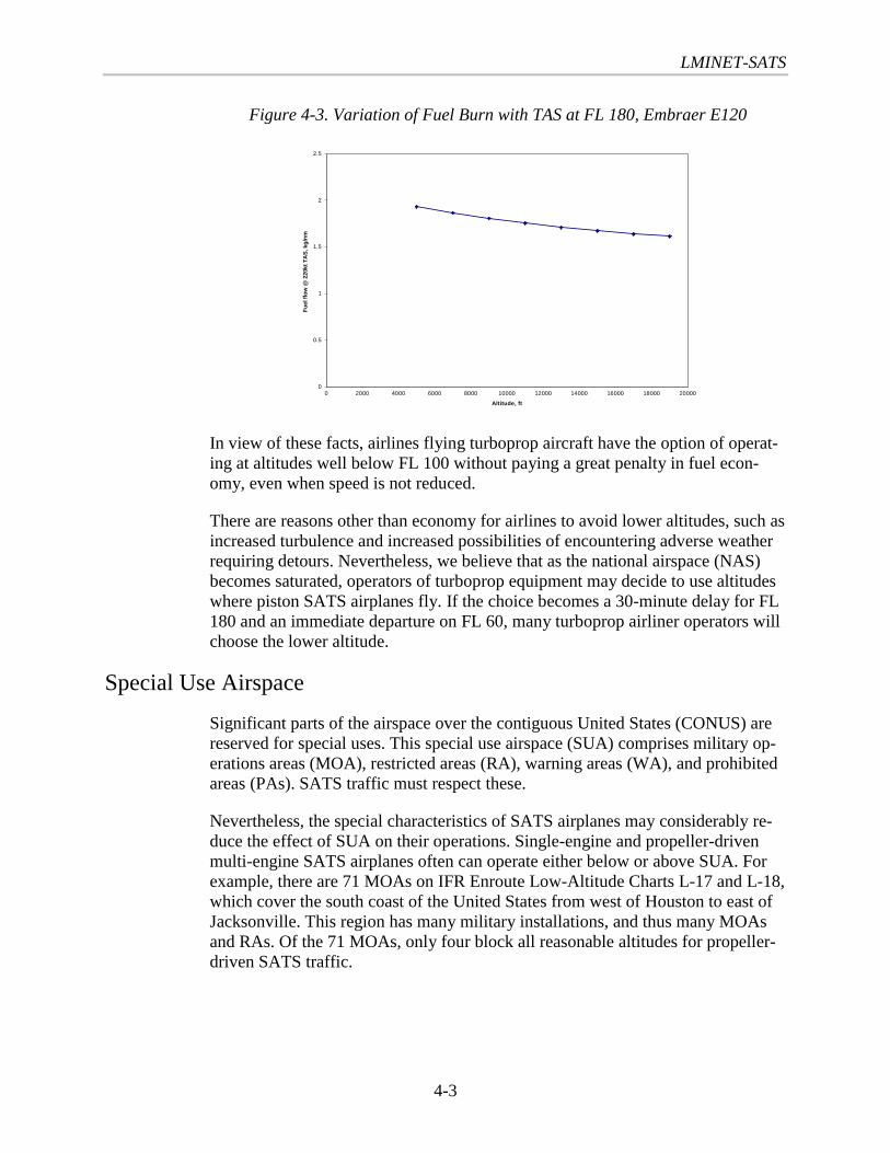
Figure 4-3. Variation of Fuel Burn with TAS at FL 180, Embraer E120

0

0.5

1

1.5

2

2.5

0 2000 4000 6000 8000 10000 12000 14000 16000 18000 20000

Altitude, ft

Fue

l flo

w @

220

kt T

AS

, kg/

nm

In view of these facts, airlines flying turboprop aircraft have the option of operat-ing at altitudes well below FL 100 without paying a great penalty in fuel econ-omy, even when speed is not reduced.

There are reasons other than economy for airlines to avoid lower altitudes, such asincreased turbulence and increased possibilities of encountering adverse weatherrequiring detours. Nevertheless, we believe that as the national airspace (NAS)becomes saturated, operators of turboprop equipment may decide to use altitudeswhere piston SATS airplanes fly. If the choice becomes a 30-minute delay for FL180 and an immediate departure on FL 60, many turboprop airliner operators willchoose the lower altitude.

Special Use Airspace

Significant parts of the airspace over the contiguous United States (CONUS) arereserved for special uses. This special use airspace (SUA) comprises military op-erations areas (MOA), restricted areas (RA), warning areas (WA), and prohibitedareas (PAs). SATS traffic must respect these.

Nevertheless, the special characteristics of SATS airplanes may considerably re-duce the effect of SUA on their operations. Single-engine and propeller-drivenmulti-engine SATS airplanes often can operate either below or above SUA. Forexample, there are 71 MOAs on IFR Enroute Low-Altitude Charts L-17 and L-18,which cover the south coast of the United States from west of Houston to east ofJacksonville. This region has many military installations, and thus many MOAsand RAs. Of the 71 MOAs, only four block all reasonable altitudes for propeller-driven SATS traffic.

4-4

Many SUAs do not operate all the time. For example, none of the four altitude-restrictive MOAs mentioned in the preceding paragraph operates continuously,and two of these never operate before 5 p.m. local time. Of 52 RAs onCharts L-17 and L-18, only 12 operate continuously and affect all propeller-SATSaltitudes.

Moreover, many SUAs have relatively small areas. For example, restricted areaR-3803A, one of the 12 continuously-operating SUAs on Charts L-17 and L-18that obstructs all reasonable propeller-SATS altitudes, can be enclosed in a rec-tangle roughly 10 nm by 5 nm.

SATS operations will begin several years after 2001, when SUA may be revisedand its area reduced. Also, the self-separating technology envisaged for SATSmay interact automatically with SUA controllers to reduce to a minimum the ef-fect of SUAs on SATS operations.

Nevertheless, in certain locations, great circle routes between SATS airports docross continuously operating SUAs that affect all altitudes. The SUA near Ed-wards AFB, east of Los Angeles and that near Holloman AFB, are examples.

On balance, we believe that it is reasonable to neglect SUA in taking a first lookat SATS traffic. A more detailed study, taking into account specific SATS sepa-ration technologies and the characteristics of specific SUAs, is desirable for morerefined discussion. As a check on the reasonableness of neglecting SUA initially,the implementation of LMINET-SATS used in this study checks traffic throughSUA near Edwards and Holloman Air Force Bases.

Mountains

Mountains would obstruct piston SATS traffic over significant portions of thewestern United States. Single-engine SATS airplanes cannot make flights on greatcircle routes between certain SATS airports in these regions. We have not ad-justed SATS trajectories for mountains for two reasons. First, in many casespasses allow SATS traffic to operate with modest increases in distance. Second,the cases where terrain interferes with great-circle operations are between lightlypopulated areas and constitute relatively small fractions of SATS operations.

SATS AND ATM STAFFING

If SATS operations can be done under Visual Flight Rules (VFR), the effect ofSATS on air traffic management will be reduced. SATS airplanes are light, so inaddition to the VFR requirement, crosswind limitations should be considered. Toget a preliminary indication of the fraction of the time that weather, including sur-face winds, will allow SATS VFR operations, we considered a trip from an air-port in the New York area, MMU, to BED near Boston.

LMINET-SATS

4-5

Our crosswind limitation was 15 knots. Although we know of no FAA or manu-facturers’ restriction on crosswind operations, light airplane makers typicallydemonstrate operations in no more than 15 knot crosswinds. Personal experiencesuggests that such winds pose a fairly significant challenge for a relatively inexpe-rienced pilot.

MMU has two runways, as does BED. Using U. S. Weather Service (OASIS) dataand taking EWR for MMU and BOS data for BED, we found that, for the calen-dar years 1981 through 1995, 90.7 percent of the time a SATS pilot would findMMU in VMC with acceptable crosswinds, and also would find BED in that statean hour later.

This example suggests that VFR SATS operations, while possible a large fractionof the time, probably are not sufficiently often available to suit the needs of busi-ness travelers. Missing or rescheduling a meeting one time out of ten is probablynot acceptable to most business people. Thus, SATS operations supporting busi-ness travel must be able to operate in IMC. It also follows that business-relatedSATS activity will require ATM staffing capable of supporting it during IMC.

The burdens that SATS operations impose on the ATM system will vary withtheir tracks. An SATS flight departing IFR from an uncontrolled airport, flying atrack that never enters airspace “owned” by a Terminal Radar Approach Control(TRACON), and landing at another uncontrolled airport presumably would re-quire services only from the low-altitude sectors through which the track passed.If the track did pass through airspace controlled by a TRACON, that TRACONwould service the flight. For example, a recent IFR flight of a Cessna 150 fromLeesburg, Virginia, (JYO) to Bradley International Airport, Windsor Locks, Con-necticut, (BDL) received services from seven different TRACONs and was con-trolled only briefly by Washington ARTCC, even though it never transited ClassB airspace.

Light airplanes regularly operate under IFR. In addition to the analysis of this traf-fic described in Chapter 3, we examined ETMS data for April 8, 1996, for indica-tions of the nature of present light-aircraft IFR flights to gain more informationabout the kinds of trips that SATS aircraft might take.

To have data for light aircraft only we considered IFR trips by Cessna 150, 152,172, 177, 180, 182, 185, and 195 airplanes, together with IFR trips by PiperCherokee (PA28) airplanes. We found ETMS records for 1,035 IFR flights be-tween 0600 EDT and 2200 EDT on that date. Some of these had intersections,rather than airports, as destinations. We ignored these because they give no indi-cations of intercity traffic. We also ignored round-robin flights with identical ori-gin and destination airports for the same reason. Certain ETMS records appearedgarbled, (e.g., an airport identifier with 9 characters) and we ignored these as well.

This left 889 flights. Figure 4-4 shows the distribution of the distances of theseflights.

4-6

Figure 4-4. Distribution of Distances of 889 IFR Flights of Light Aircraft

0

0.001

0.002

0.003

0.004

0.005

0.006

0 100 200 300 400 500 600 700 800

Distance

Pro

babi

lity

dens

ity

The probability density of Figure 4-4 has a mode near 35 nm, and another near85 nm. It is likely that the first mode largely represents training flights. The rapiddecrease in frequency of flights beyond about 100 nm may reflect light airplanespilots’ preferences for flight legs taking no longer than 1 to 2 hours.

The very small numbers of flights for distances greater than 400 nm is consistentwith confronting IFR endurance requirements with light aircraft fuel capacities.Meeting the requirement for sufficient fuel to fly to the destination, thence to analternate, and land with 45 minutes of fuel remaining, generally would limit lightaircraft to legs of about that length. Favorable winds, light loads, and pilot endur-ance may, of course, enable longer flights.

DEFINITION AND OPERATION OF LMINET-SATSLMINET-SATS provides an addition to LMINET that tracks SATS operations,and their interactions with LMINET sectors and TRACONs. It provides2,865 airports.

Input to LMINET-SATS is a list of SATS flights between SATS airports, givingorigin, destination, and starting time for each. Outputs are the number of SATSflights in each LMINET geographic sector, and in each LMINET airport’sTRACON, epoch by epoch. These traffic data may be added to LMINET trafficdata, to analyze SATS effects on the NAS.

This section gives the considerations that led to the definition of LMINET-SATS,describes its operations, and gives some example outputs.

LMINET-SATS

4-7

Considerations for Adding a SATS Underlayer to LMINET

Generally, ARTCC controllers do not handle IFR traffic below FL 100 and within30 nm of a Class A airport. Rather, controllers in the airport’s TRACON will di-rect that traffic. In some parts of the NAS, significant fractions of the airspace arewithin 30 nm of a Class A airport. Figure 4-5 shows the regions within 30 nm ofthe 64 LMINET airports.

Figure 4-5. Thirty nm Zones around LMINET Airports

The FAA’s low-altitude sectors clearly recognize the presence of TRACON air-space. TRACON airspace for Alberquerque (ABQ), Phoenix (PHX), El Paso(ELP), Chisum (CME), and Tucson (TUS) is clearly visible in Figure 4-6, whichdiagrams the low-altitude sectors for the Albuquerque ARTCC.

Figure 4-6. Low-Altitude Sectors for Albuquerque Air RouteTraffic Control Center

4-8

Users can define any partition of the NAS by a collection of points, and use theresult as en-route sectors in LMINET. All LMINET studies to date have consid-ered NAS operations many years in the future. Geographical sectors, rather thanthe present FAA sectors, were used in these studies because the studies were spe-cifically directed not to constrain operations by the present airway and sectorstructures. Sector results from these studies highlight geographic regions of heavytraffic, when traffic operates on optimal routes. Figure 4-7 shows a plan view ofbasic geographic enroute sectors used in recent LMINET studies. In most of thesestudies, heavily traveled basic sectors were viewed as divided into as many asnine subsectors.

Figure 4-7. Geographic Enroute Sectors

Because fully developed SATS will happen more than a decade in the future, webelieve that the SATS study also should use geographical sectors for air carriertraffic, at least initially. This will give consistency with previous studies, and willavoid constraining SATS operations by the airways and enroute sectors of today’sNAS.

Light-aircraft SATS operations under IFR are likely to affect TRACONs, in addi-tion to ARTCC sectors, because they typically will operate below FL 100. Ac-cordingly, we intend to use the enroute sector structure of Figure 4-8 for light-aircraft SATS operations.

LMINET-SATS

4-9

Figure 4-8. Enroute Sector Structure For Light-Aircraft SATS Operations

If the effects of SATS on workloads in the present NAS are desired, we will usethe FAA’s high-altitude sectors, shown in Figure 4-9, for air carrier traffic andturbine SATS traffic. Figure 4-6 is an example of the FAA’s low-altitude sectorsthat we will use for low-altitude SATS traffic.

Figure 4-9. FAA High-Altitude Sectors

FAA sectors are closely, and sometimes quite narrowly, linked to present J- andV- air route structures. To use the FAA sectors effectively, we will take asLMINET air carrier and SATS turbine trajectories not the wind routes used inprevious studies, but representative ETMS trajectories. Figure 4-10 shows anexample.

4-10

Figure 4-10. Example Trajectory

Light SATS traffic, however, appears likely to relate differently to the air routestructure. Light SATS trips will be short, usually not more than 300 nm, and theywill take place below FL 120. Presently, we are inclined to send light SATS traf-fic on great circle routes, perhaps avoiding TRACON airspace enroute.

Under IFR, a light-aircraft SATS flight will impose load on the sectors throughwhich it passes, either geographic or FAA, and also on the TRACONs of eachLMINET airport to which the flight gets as close as 30 nm. In some areas, notablythe mid-Atlantic coastal region, flights may be handled entirely by TRACONs.We will track SATS light-aircraft traffic separately from other TRACON trafficso that analyses may consider this traffic to be handled by separate TRACON sta-tions.

Following is a brief description of airports in LMINET-SATS, the extension ofLMINET to model SATS operations.

◆ LMINET-SATS has two airport classes, “major” and “SATS.” The majorairports are the 64 LMINET airports. The SATS airports make up a set ofabout 800 other airports. The SATS airports generally will have at leastone hard-surfaced runway not less than 2,000 feet long.

◆ Major airports’ capacity models are the present LMINET capacity models.Air carrier operations at these airports are modeled as in the presentLMINET. Because the purpose of our study is to model SATS as relief tomajor airports, SATS operations with piston aircraft do not involve majorairports. (Of course, SATS-to-major airport and major-airport-to-SATSoperations in light aircraft are possible, and they could be modeled if suchoperations did not violate the light SATS spirit.)

LMINET-SATS

4-11

◆ SATS operations with turbine equipment may involve major airports.

◆ SATS operations in IFR involve TRACONs when the route is within 30nm of a major airport. We make this stipulation because the FAA pres-ently does ATM this way.

◆ SATS airports capacity models are adapted from present LMINET airportmodels. There is no reservoir of ready-to-depart aircraft because SATSoperations are assumed to use on-base resources. Taxi-out, departure run-way, taxi-in, and arrival runway are modeled as in LMINET.

Following is a list of services required by SATS operations:

◆ Piston (four-place, single-engine piston) SATS operations

➤ SATS airport to SATS airport

■ Taxi-out;

■ Departure runway;

■ If departure airport is within 30 nm of a major airport, departureTRACON;

■ Low-altitude ARTCC subsectors where the track passes through;

■ If track passes within 30 nm of a major airport, the airport’s arrivalTRACON;

■ Arrival runway;

■ Taxi-in.

◆ Turbine SATS operations

➤ SATS airport to SATS airport

■ Taxi-out;

■ Departure runway;

■ If departure airport is within 30 nm of a major airport, departureTRACON;

■ High-altitude ARTCC subsectors where the track passes through;

■ If arrival airport is within 30 nm of a major airport, arrivalTRACON;

4-12

■ Arrival runway;

■ Taxi-in.

➤ SATS airport to major airport

■ Taxi-out;

■ Departure runway;

■ If departure airport is within 30 nm of a major airport, departureTRACON;

■ High-altitude ARTCC subsectors where the track passes through;

■ Arrival TRACON;

■ Arrival runway;

■ Taxi-in.

➤ Major airport to major airport

■ Taxi-out;

■ Departure runway;

■ Departure TRACON;

■ High-altitude sectors where the track passes through;

■ Arrival TRACON;

■ Arrival runway;

■ Taxi-in.

SATS airports

We developed a set of SATS airports in this way: The FAA’s Terminal AreaForecast (TAF) treats 3,412 airports and TRACONs. These include more than400 airports receiving FAA and contract tower and radar service, and more than3,000 other airports in the National Integrated Airport Plan. The airports are allpublic use airports, with at least one paved runway.

Not all the TAF airports are in the continental United States; however, and someof the airports listed, such as Andrews Air Force Base (ABW), are exclusivelymilitary facilities not likely to become available for SATS. Deleting the TRA-CONs, the exclusively military airports, and the 64 LMINET airports left a set of

LMINET-SATS

4-13

3, 015 airports. We chose this collection as the set of SATS airports. Their loca-tions are shown in Figure 4-11.

Figure 4-11. SATS Airports

Clearly, the SATS airports are quite widely distributed across the contiguousUnited States.

LMINET-SATS Operations

LMINET-SATS input is a file of demand for SATS flights. It is a flat ASCII file,giving a set of {epoch2, origin, destination, number of flights} quadruples. Forexample, a very short input file would be

{ {0, YIP, GAI, 1}, {0, FWA, DPA, 3}, {3, BED, LDJ,1}, {2, SGH, GAI, 1} }

That file calls for one flight from Willow Run Airport near Detroit to Montgom-ery County Airport in suburban Washington, D. C., and one flight from FortWayne, Indiana, to DuPage, Illinois, a western suburb of Chicago in epoch 0,followed by a flight from Springfield, Ohio, to Montgomery County Airport inepoch 2, and a flight from Hanscomb Field, near Boston, to Linden, New Jersey,near New York City, in epoch 33.

Up to 27,500 SATS departures may be scheduled in each epoch. For each ofthese, LMINET-SATS generates the set of LMINET sectors through which theflight would pass, and the epochs during which the flight will occupy them.

LMINET-SATS also generates the set of LMINET airports for which the flightpasses within 30 nm, and the epoch of arrival in each 30 nm ring. We believe thesedata are important because SATS flights must at least have the option of operatingunder IFR if they are to be sufficiently reliable for business travel and because the

2 LMINET operates on epochs, which may be 1 hour or 1/2 hour long. Presently 1-hour ep-

ochs are used.3 In the operating LMINET, the airport codes are replaced by integer identifying numbers.

4-14

FAA controls IFR traffic within the Mode C Veil, not via ARTCC sectors, but viathe TRACONs of the airports involved.

Presently LMINET-SATS trajectories for propeller-driven SATS airplanes aregreat circles. We assume that single-engine SATS airplanes cruise at 160 kt GS,and that piston-driven multi-engine SATS airplanes cruise at 190 kt GS.

We believe that the assumption of great circle routes for propeller-SATS airplanesis not particularly restrictive. Their trips generally are less than 320 nm, and so arenot likely to be long enough for optimization for varying wind to have significanteffects. (Please see the sections on “Special Use Airspace” and “Mountains” fordiscussions of SUA and terrain effects.)

The assumption of zero wind is somewhat restrictive. Winds aloft often reach20 percent of prop-SATS cruising speed, and in a subsequent report we will ex-tend the LMINET winds-aloft model to the altitudes at which prop-SATS flightswill operate.

For an example of the operation of LMINET-SATS, consider the flight from YIPto GAI starting in epoch 0. The first NAS facility to be affected is the DTWTRACON, in epoch 0. LMINET geographic sector 223, and the CLE TRACON,also handle the flight in epoch 0.

The flight arrives at sector 214 , passes through the PIT TRACON, and re-enterssector 214, in epoch 1. We believe that the two entries into sector 214 do not rep-resent double counting, because there would be a handoff from sector 214 to thePIT TRACON, and another from that TRACON to sector 214.

In epoch 2, the flight continues in sector 214, then enters sector 205, and, finally,enters airspace of the IAD TRACON. We believe it is reasonable to count theslow-moving prop-SATS traffic as affecting an LMINET sector during each ep-och in which it occupies the sector. Since a prop-SATS flight would occupy theMode C Veil of a given airport no longer than 22.6 minutes, even if a prop-SATSflight is in a TRACON during two epochs, we count it only in the first one.

RESULTS

In this section we discuss results of operating LMINET and the underlayer,LMINET-SATS.

An initial exercise

As an initial exercise of the SATS underlayer of LMINET, we considered fourdemand cases. Two of these were for SATS delivering 1 percent of RPM demand, in2007 and 2022. The final two cases were for SATS delivering the difference be-tween RPM demand and the RPM delivered by air carriers, enjoying the benefits ofNASA ATM technology and of new hubs, increased point-to-point routes, schedule

LMINET-SATS

4-15

smoothing, and night in 2007 and 2022. Chapter 3 explains how we developed thesedemand schedules.

WHEN SATS DELIVERS 1 PERCENT OF RPM DEMAND

Figure 4-12 shows the total number of SATS departures required to deliver 1 per-cent of demanded RPM in 2007 and 2022.

Figure 4-12. Hourly SATS Departures Required to Meet 1 Percentof RPM Demand

0

1000

2000

3000

4000

5000

6000

0 5 10 15 20 25

Baseline GA 2007 2022

These operations would substantially increase operations at several SATS airports.Nevertheless, as shown by the examples of Figures 4-13 and 4-14, for many airportsthe increases appear to be well within capacity. VNY and MMU both have fourrunways, one with ILS. VNY has a continuously operating tower; MMU’s toweroperates from 0645 to 2230, which covers all the busy periods shown in Figure 4-14.

Figure 4-13. Piston ILS Arrivals at Van Nuys, California

25

0

10

20

30

40

50

60

0 5 10 15 20

Eastern time

Hou

rly a

rriv

als

GA Baseline 2007 2022

4-16

Figure 4-14. Piston ILS Arrivals at Morristown, New Jersey

0

5

10

15

20

25

0 10 20 30

Eastern time

Ho

url

y a

rriv

als

Baseline GA 2007 2022

Now we explore the effects of SATS delivering 1 percent of demanded RPM onenroute sectors and TRACONs. We consider enroute sectors first.

Present FAA standards restrict the number of aircraft in a subsector to valuesranging from 15 to 21. Present subsectors often conform closely to present air-ways, and their boundaries may be changed. So, rather than treat any specific pre-sent sectors, we will consider what sorts of traffic densities might beaccommodated in the airspace above geographic regions, with present ATMmethods. The present LMINET-SATS results give data for sectors roughly120 nautical miles on a side.

Piston-driven SATS aircraft will not be pressurized. Accordingly, they will notoperate at altitudes above 12,000 feet MSL. Much of the CONUS has ground lev-els at or above 1,000 feet MSL. Prudent cruising altitudes probably will not be lessthan about 3,000 feet AGL, to avoid obstacles and to give reasonable opportunityfor a successful forced landing. Thus the available range of enroute altitudes forpiston SATS airplanes appears to range from 4,000 feet to 12,000 feet MSL.

With present conventions, there would be nine IFR altitudes in that range, fivewestbound and four eastbound. Many present ARTCC subsectors that are 900 to1,000 feet thick, so it seems reasonable to assume that each of the available alti-tudes could belong to a distinct sector.

Dividing a 120 nm by 120 nm square into geographic subregions could be done inmany ways; nevertheless, achieving more than about four subregions seems ques-tionable. If the division were divided into equal subsquares, each would be 60 nmon a side. Propeller SATS aircraft would transit such regions in about 22 minutes.

LMINET-SATS

4-17

It seems likely that much shorter times-in-sector would make coordination amongsector controllers difficult.

Division into subregions parallel to one pair of the original region’s sides mightbe effective in places where the SATS traffic was all headed in much the samepair of reciprocal directions. Taking these long, narrow corridor subregions lessthan about 30 nm wide makes heavy restrictions on the set of trajectories thatcould be accommodated. Propeller SATS aircraft typically would spend about40 minutes in a corridor sector.

We conclude that present ATM methods are unlikely to result in more than about36 independent subsectors in each 120 nm by 120 nm region.

If interarrival times of aircraft at a sector follow a Poisson distribution—whichETMS data indicate is the case for the present FAA sectors4—and spend 20 min-utes in the sector, then the number of aircraft in a sector at one time also will havea Poisson distribution, with mean equal to one-third the hourly arrival rate. Tokeep the number of aircraft in a sector at or below 18 with 95 percent confidence,the hourly arrival rate should not exceed 37.33. If the 120 nm by 120 nmLMINET sectors are divided into four subregions geographically, and into ninealtitude layers, the hourly arrival rate to the LMINET sector should not exceed37.33 × 36 = 1344. (That rate is an upper bound—probably a generous one—on apractical arrival rate. The FAA is not likely to put 36 controllers to work on eightthousand feet of altitude over one 120 nm by 120 nm geographic region!)

Figure 4-15 shows hourly demands for certain LMINET sectors approach one-third of the theoretical maximum, when SATS aircraft deliver 1 percent of theRPM demanded in 2007. The figure also shows only SATS traffic, but there willbe other demands for ATM services. As we noted above, saturation of enroutesectors in Class A airspace (above 18,000 feet) may cause operators of turboproptransports to use lower altitudes.

4 Lee, D. A. et al., “Technical and Economic Analysis of Air Transportation Management Is-

sues Related to Free Flight,” Logistics Management Institute Report NS501T1, McLean, VA, Feb-ruary 1997.

4-18

Figure 4-15. Hourly Demand For Busy Sectors, 2007

0

200

400

600

800

1000

1200

1400

1600

0 5 10 15 20 25

Eastern time

A/C

per

hou

r

Sector 205 Maximum Sector 223

Theoretical maximum

The burden imposed by SATS aircraft on certain TRACONs also is significant.When an IFR flight is within the mode C veil of an airport with Class B airspace,that airport’s TRACON handles the flight. We computed SATS TRACONdemands as a fraction of maximum hourly operations for several airports, takingthe LMINET capacity for an airport as a measure of that maximum. Figure 4-16shows the results.

Figure 4-16. SATS TRACON Demands, 2007

0

0.2

0.4

0.6

0.8

1

1.2

1.4

0 5 10 15 20 25

Eastern time

Fra

ctio

n of

max

imum

ope

ratio

ns

EWR MCO MKE MDW

LMINET-SATS

4-19

Figures 4-15 and 4-16 strongly suggest that delivering 1 percent of demandedRPM by SATS in 2007 would pose significant, but probably not impossible,demands on air traffic management by present methods.

Now we consider when SATS delivers 1 percent of demand in 2022. Figures 4-17and 4-18 update Figures 4-15 and 4-16, respectively, to that year.

Figure 4-17. Hourly Demand For Busy Sectors, 2022

0

200

400

600

800

1000

1200

1400

1600

0 5 10 15 20 25

Eastern time

A/C

per

hou

r

Sector 205 Maximum Sector 223

Theoretical maximum

Figure 4-18. SATS TRACON Demands, 2022

0

0.2

0.4

0.6

0.8

1

1.2

1.4

1.6

1.8

2

0 5 10 15 20 25

Eastern time

Fra

ctio

n o

f ma

xim

um o

per

atio

ns

EWR MCO MKE MDW

4-20

At the 2022 levels, the demands for both sector and TRACON services made bySATS aircraft meeting 1 percent of RPM demand are great enough to raisequestions about satisfying them with present ATM methods. Sector effects reach70 percent of the theoretical maximum, and TRACON effects substantiallyexceed the demands made by arriving and departing flights when certain airportsare working to capacity.

We also considered arrivals to SATS airports close to major terminals. Figure 4-19shows hourly IFR arrivals to the 14 SATS airports within 30 nm of EWR (TEB,MMU, CDW, LDJ, 39N, N52, N07, 6N4, N51, 4N1, 47N, 3N6, JRB, and 6N5).

Figure 4-19. Hourly Piston-SATS Arrivals to SATS Airports Near EWR

0

10

20

30

40

50

60

70

80

90

0 5 10 15 20 25

Eastern time

Hou

rly a

rriv

als

Baseline GA 2007 2022

These arrivals may be more burdensome to the EWR TRACON than SATSflights that only transition TRACON airspace during cruise.

Effects of Improved Strategies

What are the effects of ATM when SATS delivers the difference between theRPM that travelers would consume absent any constraints by carriers’ interests orNAS properties? What could be delivered if economically motivated carriers useimproved strategies (e.g., new hubs, more direct flights, schedule smoothing, andnight flights) in a NAS if certain NASA decision-support tools for ATM (e.g.,TMA, MCTMA, A/PFAST, SMA/SMS, T-NASA, AVOSS, ROTO, DROM, andSVS) are fully implemented? Figure 4-20 shows the overall possible level ofoperations.

LMINET-SATS

4-21

Figure 4-20. SATS Operations to Supply RPM Deficit

0

1000

2000

3000

4000

5000

6000

7000

8000

9000

10000

0 5 10 15 20 25

GA Baseline 2007 2022

In 2007, the RPM deficit is small. SATS needs to provide even less than the 1percent of RPM considered earlier. But in 2022, many more SATS operations arerequired.

All traffic measures considered in the 1 percent cases are greatly increased for2022. Figure 4-21 shows examples of arrivals to VNY. The peak level of120 hourly arrivals would be difficult to sustain with VNY’s present two runways.

Figure 4-21. Piston-SATS Arrivals to VNY, Deficit Case

VNY

0

20

40

60

80

100

120

140

0 5 10 15 20 25

Eastern time

Hou

rly a

rriv

als

Figure 4-22 compares piston-SATS arrivals to Sector 205 when SATS makes upthe deficit between RPM supplied by profit-motivated carriers using the NAS im-

4-22

proved by NASA tools, and also using improved carrier strategies, and the RPMforecast of the FAA TAF.

Figure 4-22. Arrivals to Sector 205

0

500

1000

1500

2000

2500

0 5 10 15 20 25

GA Baseline 2022 Default Th. Maximum

Theoretical Maximum

The highest demand levels would be difficult to sustain with present ATM methods.

Figure 4-23 shows hourly demand for piston-SATS arrivals at the 14 airports(other than major airports) located within 30 nm of EWR.

Figure 4-23. Arrivals To SATS Airports Near EWR, Deficit Case

0

20

40

60

80

100

120

140

160

180

0 5 10 15 20 25

Eastern time

Ho

url

y a

rriv

als

Baseline GA 2022 deficit

LMINET-SATS

4-23

Conclusions

In view of these early results on the demands that piston-SATS traffic wouldmake on the ATM system, we make the following conclusions:

◆ SATS might deliver economically significant levels of RPM in 2007,while still supported by present ATM methods. The levels of traffic wouldnot change materially the total RPM delivered by the air transport system.

◆ New ATM methods almost certainly would be required for SATS to de-liver a significant fraction of total RPM provided by the air transport sys-tem in 2022. Some facilities, such as runways at certain SATS airports,might be taxed beyond their capacities when SATS functions at such alevel.

5-1

Chapter 5

Summary and Future Work

The models presented in this report are powerful tools policy decision makers canuse for air traffic system planning, especially in SATS planning. The models helppredict SATS demand for airports and airspace. They are flexible, parameterized,easy-to-use tools to predict SATS demand in different scenarios, as shown by ourcase studies.

Readers should be aware that the figures we present in this report are notforecasts; they are the results of “what-if” studies to demonstrate the use of ourmodels. The models, albeit developed with empirical data fitting and flexibility tochange the parameters, are not the forecast models. They are “what-if” analysistools. Our models can predict SATS demand based on the assumed scenarios. Themodels are constructed for easy link to any SATS demand forecast models, whichmay come from different sources.

In light of the current model development, our future emphasis will be estimationof the SATS demand curve, which will quantify the SATS demand for a given setof socioeconomic parameters, and a set of SATS performance and cost parame-ters. With completed SATS-FDM and LMINET-SATS for the SATS airspacedemand, our future work should be the SATS demand model on a higher aggre-gate level, dealt with by SATS-ADM. Specifically, we need to develop a quantita-tive model of SATS operations for each aircraft type for each airport.

After we construct the SATS demand curve, we can use the model to analyze theeffect of SATS on demography and economy in the area surrounding an airport.On another hand, SATS will have an impact on demography and economy in thearea surrounding an airport. This will require a feedback loop in analyzing SATSdemand and demography and economy. With the closed loop, we will completethe SATS demand model development.

The model will assume that air travels are induced economic activities that mustsatisfy basic economic laws. Predicted travel is the point where the demand curveand the supply curve meet. Generally, the mathematical model takes the followingform:

),( parameterstravelofcostparametersmicsocioeconofT = , [Eq. 5-1]

whereT is the measure of travel such as TPM defined in Chapter 2, for a city pair,for the total travel out of a city, or the total travel in a region such as the UnitedStates. A commercial air traffic example is the Air Carrier Investment Model(ACIM) in the Aviation System Analysis Capacity (ASAC) model suite. In

5-2

ACIM, T is the total U.S. RPM; the socioeconomic parameters are population, percapita income, and unemployment rate; the cost of travel is in revenue per seatmile (RSM), which depends on numerous costs for labor, material, maintenance,and acquisition, plus others; and competition in the marketplace measured in mar-ket share and the Herfindahl index.

Typically, to facilitate the parameter estimation, a linear model is assumed, al-though the products of variables frequently are included. If the model takes a log-linear form, then the parameters estimated are the elasticities (e.g., traffic willgrow 2 percent for each 1 percent of per capita income growth if the elasticity ofper capita income is 2.0, assuming all other factors hold constant).

After model parameters, or, more likely, elasticities, are estimated, we can ana-lyze many what-if scenarios using various socioeconomic and cost parameters.This methodology has been successfully employed to assess the effect of trafficon air carrier business strategies and ATM technologies ([1,2]. Historical data arerequired to construct such a model. For example, the Forms 41 data from the De-partment of Transportation, 1985 through 1994, at the largest 85 U.S. domesticairports by all airlines are used to estimate the parameters in ACIM. No historicaldata for SATS exist. If we used models such as ACIM for forecasting SATS de-mand by varying the input variables, we would implicitly assume that the modelstructure will be intact even with different sets of input and output variables. TheSATS economic demand model must be different, in both mathematical form andthe values of elasticities , because it is a different mode of transportation. It is notpossible to borrow one model in another mode of transportation, or to use an oldmodel after the industry experiences structural change. An example is exponentialgrowth of commercial air traffic offered by air carriers and the gradual decline ofGA traffic in the past two decades in the United States.

It is not plausible to use historical GA data to build a SATS traffic demand modelbecause the two are different travel options. The proposed SATS will be morecost-effective to acquire and operate, faster and easier to operate, and require lesspilot training.

Building such a model will be a challenging, creative task. A set of modelingprinciples will help in our modeling:

◆ The model must be based on sound economic principles.

◆ The model must use the available data fully.

◆ The model must be as comprehensive as possible to consider potentialSATS demand scenarios, which will consider diverted demand fromcommercial travel, latent demand, and mode selection of all transportationmeans including ground-based.

◆ The model is best constructed by linking a set of component models.

Summary and Future Work

5-3

◆ If one component model is unavailable, the hooks for its later connectionand appropriate default values must be provided. Furthermore, the mod-eler must identify the mechanism and the data needed to construct themissing component model.

◆ To capture the essence of SATS demand, the model should be as simple aspossible. The model should have as few adjustable parameters as possiblebecause each adjustable parameter in the model represents a subjective in-put and a source of uncertainty. This principle is not inconsistent with theneed for a comprehensive model. While the need for a comprehensivemodel includes all demand sources, the need for a simple model gives pri-ority to simplicity over complexity in mathematical equations, especiallyin light of the uncertainties of SATS demand functions.

◆ Adjustable parameters in the model must be interpreted easily. Ideally,they should serve as the hooks of the connection so that running the modelinvolves picking values in a set of well understood parameters, which canbe further determined by component models.

Ref-1

References

[1] Peter F. Kostiuk, Eric M. Gaier, and Dou Long, “The Economic Impacts ofAir Traffic Congestion,” Air Traffic Control Quarterly, Vol. 7(2), 1999,pp. 123–145.

[2] Logistics Management Institute,A Method for Evaluating Air Carrier Op-erational Strategies and Forecasting Air Traffic with Flight Delay, DouLong, et al., October 1999.

[3] NASA, A Method for Making Cross-Comparable Estimates of the Benefitsof Decision Support Technologies for Air Traffic Management, NASA Con-tractor Report 208455, David A. Lee, Dou Long, Melvin R. Etheridge,Joana R. Plugge, Jesse P. Johnson, and Peter F. Kostiuk, 1998.

[4] NASA, Modeling Air Traffic Management Technologies with a QueuingNetwork Model of the National Airspace System, NASA Contractor Report208988, Dou Long, David A. Lee, Jesse P. Johnson, Eric M. Gaier, and Pe-ter F. Kostiuk, 1998.

[5] NASA, A Method for Forecasting the Commercial Air Traffic Schedule inthe Future, NASA Contractor Report 208987, Dou Long, David A. Lee, EricM. Gaier, Jesse P. Johnson, Peter F. Kostiuk, 1998.

[6] NASA, Aviation System Capacity Program, Advanced Air TransportationTechnologies,ATM Definition, Volume 1, Current and Future OperationalConcepts for the National Airspace System, Volume 2, Coverage of FutureNational Airspace Operational Requirement, October 21, 1997.

[7] NASA, National General Aviation Roadmap—Definition Document for aSmall Aircraft Transportation System Concept, Bruce Holmes, NASA Gen-eral Aviation Program Office, Langley Research Center, March 4, 1999.

[8] NASA, Small Aircraft Transport System—Strawman Features & Capabili-ties, Office of Aeronautics and Space Transportation Technology

[9] Federal Aviation Administration,National Plan of Integrated Airport Sys-tems (1998–2002) (NPIAS), March 1999, Washington, D.C.

[10] Federal Aviation Administration,General Aviation and Air Taxi ActivitySurvey (GAATA), Statistics and Forecast Branch, Planning Analysis Divi-sion, Office of Aviation Policy and Plans, March 1999, Washington, D.C.

Ref-2

[11] Federal Aviation Administration,National Airspace System Architecture,Office of System Architecture and Investment Analysis (ASD-1), 800 Inde-pendence Avenue, SW, Washington, D.C., December 1997.

[12] Federal Aviation Administration,FAA Long-Range Aviation Forecasts Fis-cal Years 2010, 2015, and 2020, Office of Aviation Policy and Plans, 800Independence Avenue, SW, Washington, D.C., June 1998.

[13] Department of Transportation,FAA Aerospace Forecasts—Fiscal Years1999–2010, Report No. FAA APO-99-1, Federal Aviation Administration,Office of Aviation Policy and Plans, Statistics and Forecast Branch, Wash-ington, D.C., March 1999.

[14] Federal Aviation Administration,Airport Capacity Enhancement Plan, 800Independence Avenue, SW, Washington, D.C., 1998.

[15] Bureau of Transportation Statistics,The 1995 American Travel Survey,4007th Street, S.W., Suite 3430, Washington, D.C., 20590.

[16] American Airlines,Free Flight: Preserving Airline Opportunity, CaptainRussell G. Chew, September 1997.

[17] Boeing,2000 Current Market Outlook, Boeing Commercial Airplane GroupMarketing, P.O. Box 3707, Seattle, WA 98124–2207.

[18] Salah G. Hamzawi, “Lack of Airport Capacity: Exploration of AlternativeSolutions,”Transportation Research, Vol. 26A, No.1, 1992, pp. 47–58.

[19] Moshe Ben-Akiva, and Steven R. Lerman,Discrete Choice Analysis: Theoryand Application to Travel Demand, The MIT Press, Cambridge, Massachu-setts, 1985.

[20] Kenneth J. Button,Transport Economics, 2nd Edition, Edward Elgar Publish-ing Company, Brooksfield, Vermont, 1992.

[21] Kenneth Train,Theory, Econometrics, and an Application to AutomobileDemand, The MIT Press, Cambridge, MA, 1986.

[22] Kenneth Train, “The Potential Market for Non-Gasoline-Powered Automo-bile,” Transportation Research, Vol. 14A, 1980, pp. 405–414.

[23] Steven D. Beggs, and N. Scott Cardell, “Choice of Smallest Car by Multi-Vehicle Households and the Demand for Electric Vehicles,”TransportationResearch, Vol. 14A, 1980, pp. 389–404.

[24] Adib Kanafani,Transportation Demand Analysis, McGraw-Hill, New York,1983.

References

Ref-3

[25] Kingsley E. Haynes and A. Stewart Fotheringham,Gravity and Spatial In-teraction Models,Sage Publications, Beverly Hills, California, 1985.

[26] Mokhtar S. Bazaraa and C.M. Shetty,Nonlinar Programming,Johjn Wiley& Sons, New York, 1979.

A-1

Appendix A

Parameter Estimation of the Gravity Model

To use the gravity model to derive the O&D traffictij, i,j = 1, 2…N, we must firstcalibrate the model to get the parametersai, bi, i = 1, 2…N, which are based onthe conservation equation, Equation 3-3. If the coupling parametercij is deter-mined by the distance between two airports as given by Equation 3-6, then

cij = cji, i, j = 1, 2, ...,N [Eq. A-1]

cij ≥ 0, i, j = 1, 2,…,N, [Eq. A-2]

cii = 0, i = 1, 2,…,N. [Eq. A-3]

sincedij = dji, andf( ⋅ ) ≥ 0 andf(0) = 0 by our assumption. If the coupling pa-rameterscij, i, j = 1, 2,…,N, are symmetric, then

ai = bi, i = 1, 2,…,N. [Eq. A-4]

Thus, the gravity model can be restated as

,,...,2,1,, NjiTaTact jjiiijij =⋅⋅⋅⋅= [Eq. A-5]

satisfying

∑ ==⋅⋅⋅⋅j

ijjiiij NiTTaTac .,...,2,1, [Eq. A-6]

If we assume uniformity, i.e.,

ai = aj = a, i, j = 1, 2,...,N, [Eq. A-7]

then by summing all the equations fori= 1 throughN, we get

∑∑ =⋅i

ijji

iij TTTca,

2 [Eq. A-8]

or

jji

iij

ii

TTc

T

a⋅

=∑

∑

,

[Eq. A-9]

A-2

Although this is a popular method to estimate the parameters, it does not yieldsatisfactory calibration. However, it does serve as a starting point for other meth-ods based on iteration.

Let

,,...,2,1,0 NiTax iii =≥⋅= [Eq. A-10]

then the calibration function of the gravity model is

∑ ==⋅j

ijiji NiTxcx .,...,2,1, [Eq. A-11]

By rearranging Equation A-11, we get

.,...,2,1, Nixc

Tx

jjij

ii =

⋅=∑

[Eq. A-12]

This is a direct substitution method to solve the nonlinear equation, i.e.,

,,...,2,1,)(

)1( Nixc

Tx

j

kjij

ikii

=⋅

=∑

+ [Eq. A-13]

wherexi(k) is thekth iteration ofxi. Although simple and straightforward, this

method does not yield a convergent solution because it is not a contraction map-ping (proof omitted).

Let

∑ ==−⋅=j

ijijii NiTxcxF ,,...,2,1,0 [Eq. A-14]

andF = (F1, F2, …, FN)t. The Newton-Ralphson method, a popular way to findthe roots of nonlinear Equation A-11, is given by

,,...,2,1,)()()1( Nixxx ki

ki

ki =δ+=+ [Eq. A-15]

whereδx=(δx1, δx2, …, δxN)t is the solution of the linear equation

.FxJ −=δ⋅ [Eq. A-16]

J is the Jacobian matrix ofF, defined as

.,...,2,1,, Njix

FJ

j

iij =

∂∂

= [Eq. A-17]

Appendix A: Parameter Estimation of the Gravity Model

A-3

Substituting Equation A-11 for Equation A-17 yields

.,...,2,1,, NjicxJ ijiij =⋅= [Eq. A-18]

If Equation A-17 is substituted in Equation A-16, we get

,,...,2,1,)()()()( NiTxcxxcxj j

ik

jijkk

jijk

i i=+⋅−=⋅∑ ∑δ [Eq. A-19]

or

( ) ,,...,2,1,)()()( NiTxxcx ik

jk

jj

ijk

i ==+∑ δ [Eq. A-20]

or

∑ ==⋅ +

ji

kjij

ki NiTxcx .,...,2,1,)1()( [Eq. A-21]

In terms of matrices,

( ) ,)1( kk dxC =⋅ + [Eq. A-22]

whered(k) = (d1, d2, …, dN)t, and

.,...,2,1, Nix

Td

i

ii == [Eq. A-23]

Then,

.)(1)1( kk dCx ⋅= −+ [Eq. A-24]

In theory, if we can carry the iteration forward, eventually we will get the conver-gence and solve the nonlinear equation. In practice, this iteration scheme does notwork because it requires taking the inverse of a large dimension matrix(2,865×2,865). It is impractical even if we solve the linear equationEquation A-21 directly through the LU decomposition because it requires manyiterations to solve the nonlinear equations. We must seek another solution.

It is not necessary to force the conservation equation, Equation A-6, strictly incalibrating the gravity model because our GA network, although comprehensive,still leaves about 8 percent of GA traffic uncovered. Undoubted this traffic willcome to our GA network airports. Understanding this, we can restate the gravitycalibration problem as a nonlinear programming problem:

A-4

∑=i

isxf 2)(:min [Eq. A-25]

subject to: ,,...,2,1, NiTsxcx iij

jiji ==−⋅∑ [Eq. A-26]

and

.,...,2,1,0 Nixi =≥

s is a vector of slack variables. Obviously, whens = 0, we get the exact solutionfor the gravity calibration. In practice, we need only to minimize the objectivefunctionf(x) until the convergence is found. For this report, we used the followingcriterion:

ε<

i

i

T

smax [Eq. A-27]

and we selectε to be 0.05, well within the range of 8 percent implied by the data.

We used the deepest decent method to solve the nonlinear programming [26]. Theiteration is carried by the following:

( )( ))()()1( kkk xfhxx ∇−=+ [Eq. A-28]

where∇(⋅) is the gradient of the objective function f(⋅) andh represent the scalarstep size. The optimal step size can be determined using the following formula:

( ) ( )( ) ( ) ( ))()()(

)()(

kktk

ktk

xfxHxf

xfxfh

∇∇

∇⋅∇= . [Eq. A-29]

By definition,

t

ixfxf

xf

∂∂=∇

)(

)()( [Eq. A-30]

and from Equation A-25,

∑ ∂∂=

∂∂

i k

ii

k x

ss

xf

xf2

)(

)(. [Eq. A-31]

Appendix A: Parameter Estimation of the Gravity Model

A-5

By Equation A-26,

∑

∑=⋅

≠⋅

=

−

∂∂=

∂∂

jjkj

iki

jijiji

kk

i

ikxc

ikcx

Txcxxx

s

,

,

[Eq. A-32]

If we substitute Equation A-32 into Equation A-31, we get

⋅⋅+⋅=

∂∂

∑∑i

ikiij

jkjkk

cxsxcsx

xf2

)(

⋅⋅+⋅⋅= ∑∑ ii

iikjk

jjk xscxsc2

∑ +=i

ikiik xssc )(2 . [Eq. A-33]

The Hessian matrixH = (Hij) is defined as the second derivative of the objectivefunctionf. By Equation A-33,

,3212

1

2

1HHH

xx

fH

lkkl ++=

∂∂∂= [Eq. A-34]

where

∑ ∂∂

=i

il

iki x

x

scH1

∑∑ ⋅⋅+=i

ilikij

jljkl xccxcc

∑ ∑ ⋅⋅+⋅⋅=i i

ilikiilikl xccxcc

∑ +=i

ikikili xccc )( . [Eq. A-35]

A-6

∑ ∑

∑

=

⋅

≠⋅⋅

=

i jjljki

ikikkl

klxcc

klcxc

H

.,

,,

2 [Eq. A-36]

( )lkkl sscH +=3 . [Eq. A-37]

After we know the gradient vector and the Hessian matrix, we can carry out itera-tion according to the deepest decent algorithm.

There is excessive computation in computing the optimal step size. It is faster touse a fixed step size, which is determined by trial and error. We found 4.0× 10–6

is the largest step size without jeopardizing the convergence of solution.

REPORT DOCUMENTATION PAGE Form ApprovedOMB No. 0704-0188

Public reporting burden for this collection of information is estimated to average 1 hour per response, including the time for reviewing instructions, searching existing datasources, gathering and maintaining the data needed, and completing and reviewing the collection of information. Send comments regarding this burden estimate or any otheraspect of this collection of information, including suggestions for reducing this burden, to Washington Headquarters Services, Directorate for Information Operations andReports, 1215 Jefferson Davis Highway, Suite 1204, Arlington, VA 22202-4302, and to the Office of Management and Budget, Paperwork Reduction Project (0704-0188),Washington, DC 20503.1. AGENCY USE ONLY (Leave blank) 2. REPORT DATE

June 20013. REPORT TYPE AND DATES COVERED

Contractor Report4. TITLE AND SUBTITLE

A Small Aircraft Transportation System (SATS) Demand Model5. FUNDING NUMBERS

C NAS2-14361

6. AUTHOR(S)

Dou Long, David Lee, Jesse Johnson, and Peter KostiukWU 522-99-11-01

7. PERFORMING ORGANIZATION NAME(S) AND ADDRESS(ES)Logistics Management Institute2000 Corporate RidgeMcLean, Virginia 22102-7805

8. PERFORMING ORGANIZATIONREPORT NUMBER

LMI-NS004S1

9. SPONSORING/MONITORING AGENCY NAME(S) AND ADDRESS(ES)National Aeronautics and Space AdministrationLangley Research CenterHampton, VA 23681-2199

10. SPONSORING/MONITORINGAGENCY REPORT NUMBER

NASA/CR-2001-210874

11. SUPPLEMENTARY NOTES

Langley Technical Monitor: Robert YackovetskyFinal Report

12a. DISTRIBUTION/AVAILABILITY STATEMENT

Unclassified-UnlimitedSubject Category 05 Distribution: NonstandardAvailability: NASA CASI (301) 621-0390

12b. DISTRIBUTION CODE

13. ABSTRACT (Maximum 200 words)The Small Aircraft Transportation System (SATS) demand modeling is a tool that will be useful for decisionmakersto analyze SATS demands in both airport and airspace. We constructed a series of models following the general top-down, modular principles in systems engineering. There are three principal models, SATS Airport Demand Model(SATS-ADM), SATS Flight Demand Model (SATS-FDM), and LMINET-SATS. SATS-ADM models SATSoperations, by aircraft type, from the forecasts in fleet, configuration and performance, utilization, and trafficmixture. Given the SATS airport operations such as the ones generated by SATS-ADM, SATS-FDM constructs theSATS origin and destination (O&D) traffic flow based on the solution of the gravity model, from which it thengenerates SATS flights using the Monte Carlo simulation based on the departure time-of-day profile. LMINET-SATS, an extension of LMINET, models SATS demands at airspace and airport by all aircraft operations in U.S.The models use parameters to provide the user with flexibility and ease of use to generate SATS demand fordifferent scenarios. Several case studies are included to illustrate the use of the models, which are useful to identifythe need for a new air traffic management system to cope with SATS.

14. SUBJECT TERMS

Small Aircraft Transportation System, SATS, LMINET, LMINET-SATS, air15. NUMBER OF PAGES

77transportation demand model, gravity model 16. PRICE CODE

17. SECURITY CLASSIFICATIONOF REPORT

Unclassified

18. SECURITY CLASSIFICATIONOF THIS PAGE

Unclassified

19. SECURITY CLASSIFICATIONOF ABSTRACT

Unclassified

20. LIMITATIONOF ABSTRACT

UL

NSN 7540-01-280-5500 Standard Form 298 (Rev. 2-89)Prescribed by ANSI Std. Z-39-18298-102