a smoothed particle hydrodynamic simulation utilizing the parallel
TRANSCRIPT
Department of Science and Technology Institutionen för teknik och naturvetenskap Linköping University Linköpings Universitet SE-601 74 Norrköping, Sweden 601 74 Norrköping
LiU-ITN-TEK-A--09/052--SE
A smoothed particlehydrodynamic simulation
utilizing the parallelprocessing capabilities of the
GPUsViktor Lundqvist
2009-09-30

LiU-ITN-TEK-A--09/052--SE
A smoothed particlehydrodynamic simulation
utilizing the parallelprocessing capabilities of the
GPUsExamensarbete utfört i vetenskaplig visualisering
vid Tekniska Högskolan vidLinköpings universitet
Viktor Lundqvist
Handledare Magnus WrenningeExaminator Jonas Unger
Norrköping 2009-09-30
Upphovsrätt
Detta dokument hålls tillgängligt på Internet – eller dess framtida ersättare –under en längre tid från publiceringsdatum under förutsättning att inga extra-ordinära omständigheter uppstår.
Tillgång till dokumentet innebär tillstånd för var och en att läsa, ladda ner,skriva ut enstaka kopior för enskilt bruk och att använda det oförändrat förickekommersiell forskning och för undervisning. Överföring av upphovsrättenvid en senare tidpunkt kan inte upphäva detta tillstånd. All annan användning avdokumentet kräver upphovsmannens medgivande. För att garantera äktheten,säkerheten och tillgängligheten finns det lösningar av teknisk och administrativart.
Upphovsmannens ideella rätt innefattar rätt att bli nämnd som upphovsman iden omfattning som god sed kräver vid användning av dokumentet på ovanbeskrivna sätt samt skydd mot att dokumentet ändras eller presenteras i sådanform eller i sådant sammanhang som är kränkande för upphovsmannens litteräraeller konstnärliga anseende eller egenart.
För ytterligare information om Linköping University Electronic Press seförlagets hemsida http://www.ep.liu.se/
Copyright
The publishers will keep this document online on the Internet - or its possiblereplacement - for a considerable time from the date of publication barringexceptional circumstances.
The online availability of the document implies a permanent permission foranyone to read, to download, to print out single copies for your own use and touse it unchanged for any non-commercial research and educational purpose.Subsequent transfers of copyright cannot revoke this permission. All other usesof the document are conditional on the consent of the copyright owner. Thepublisher has taken technical and administrative measures to assure authenticity,security and accessibility.
According to intellectual property law the author has the right to bementioned when his/her work is accessed as described above and to be protectedagainst infringement.
For additional information about the Linköping University Electronic Pressand its procedures for publication and for assurance of document integrity,please refer to its WWW home page: http://www.ep.liu.se/
© Viktor Lundqvist

ABSTRACT
Simulating fluid behavior has proven to be a demanding challenge which requires
complex computational models and highly efficient data structures. Smoothed
Particle Hydrodynamics (SPH) is a particle based computational model used to
simulate fluid behavior that has been found capable of producing convincing results.
However, the SPH algorithm is computational heavy which makes it cumbersome to
work with.
This master thesis describes how the SPH algorithm can be accelerated by utilizing
the GPU’s computational resources. It describes a model for how to distribute the
work load on the GPU and presents a suitable data structure. In addition, it proposes
a method to represent and handle moving objects in the fluids surroundings. Finally,
the performance gain due to the GPU is evaluated by comparing processing times
with an identical implementation running solely on the CPU.


ACKNOWLEDGMENTS
I would like to thank everyone at Sony Pictures Imageworks, especially the
application group, for giving me this opportunity and making me feel part of their
team. A special thank to my supervisor Magnus Wrenninge who has been an
invaluable discussion partner and a great support all through the work on this thesis.
I am also deeply grateful to Anders Ynnerman and Aida Vitoria at Linköping’s
University who helped me to get into the IPAX program. Thank you!

CONTENTS
INTRODUCTION ............................................................................................................ 2
1. 1 MOTIVATION ..................................................................................................................... 2 1.2 WORK ENVIRONMENT ......................................................................................................... 3 1.3 OUTLINE OF REPORT ............................................................................................................ 3
BACKGROUND & RELATED WORK ................................................................................. 4
2.1 RELATED WORK .................................................................................................................. 4 2.2 SMOOTHED PARTICLE HYDRODYNAMICS (SPH) ........................................................................ 5 2.2.1 Modeling Fluid Dynamics ........................................................................................... 6 2.2.2 Smoothing Kernels ...................................................................................................... 9 2.3 COMPUTE UNIFIED DEVICE ARCHITECTURE (CUDA) ................................................................ 10 2.3.1 NVIDIA’s Hardware Architecture ............................................................................... 10 2.3.1.1 Execution Model..................................................................................................... 10 2.3.2 Programming Interface ............................................................................................. 12
IMPLEMENTATION ..................................................................................................... 14
3.1 SPH ALGORITHM .......................................................................................................... 14 3.1.1 Data Structure ........................................................................................................... 15 3.1.2 SPH and Parallel Processing ...................................................................................... 16 3.1.2 Normalize Density ..................................................................................................... 19 3.1.3 Smoothing Kernels .................................................................................................... 19 3.2 INTEGRATION METHOD ...................................................................................................... 20 3.2.1 Step Size .................................................................................................................... 20 3.3 PARTICLE SOURCES ...................................................................................................... 21 3.4 COLLISION DETECTION ....................................................................................................... 21 3.4.1 Collision Objects ........................................................................................................ 21 3.4.2 Collision Algorithm .................................................................................................... 22
RESULTS ..................................................................................................................... 24
4.1 PARTICLE BEHAVIOR .......................................................................................................... 24 4.2 PERFORMANCE.............................................................................................................. 26 4.3 DISCUSSION ..................................................................................................................... 27 4.4 FURTHER IMPROVEMENTS .................................................................................................. 28 4.4.1 Performance Improvements ..................................................................................... 28 4.4.2 Functionality ............................................................................................................. 29
REFERENCES ............................................................................................................... 31
CHAPTER 1
INTRODUCTION
This chapter aims to introduce the reader to the purpose and the underlying structure of
this thesis.
1. 1 MOTIVATION The motion of fluids has proven to be one of the most challenging physical phenomena
to simulate. The complex behavior and physical relations involved in e.g. a raising pillar
of smoke, the breaking of an ocean wave or water being poured into a glass is probably
what is making it fascinating to watch. However, mimicking these behaviors in computer
graphics requires complex computational models and highly efficient data structures. Smoothed Particle Hydrodynamics (SPH) is a particle based computational model used
to simulate fluid dynamics. The SPH model has been found capable of producing
convincing and physically based computer animations of fluid dynamics. However, the
computational burden of fluid simulation is heavy which generally results in low frame
rates. Therefore, fluid phenomena are typically simulated off‐line and then rendered in a
second step. The high simulation time together with the difficulties of predicting fluids
behavior makes it somewhat frustrating to work with, since it is often necessary to re‐
run a simulations several times in order to achieve the desired result.
During the last years the performance growth of single core contemporary general‐
purpose processors (CPUs) has stagnated. This has led to an increased interest in
multicore chip organizations, a field that the vendors of graphics processors (GPUs) have
put a lot of research into. Today’s GPUs provides a vast number of simple but deeply
multithreaded cores with high internal memory bandwidth. Although, GPUs traditionally
have been dedicated to strictly processing data strongly coupled to the rendering
process, last year’s development have led to increased programmability capabilities,
making them attractive for non‐graphical purposes. The SPH simulation algorithm is in
many ways suitable for parallel processing.
The purpose of this thesis is to examine how the computational resources on a
modern graphic card can be utilized in order to speed up the process of an SPH
simulation.
2
1.2 WORK ENVIRONMENT The main work of this thesis was carried out during an internship at Sony Pictures
Imageworks. The SPH simulation was implemented to suite the production pipeline at
Sony Picture Imageworks with the aim to be useful in future productions.
The resulting simulation tool is written as a plug‐in to the 3D visual effects program
Houdini, coded in C++ and Compute Unified Device Architecture (CUDA). CUDA is a
general purpose GPU programming language developed by NVIDIA in order to provide
users with extended control over the processing capabilities of the GPU. See section 2.3
for a detailed description of CUDA. Sony also provided several in‐house C++ libraries
facilitating certain processes, such as handling field data.
1.3 OUTLINE OF REPORT Chapter 2 consists of the background information and previous work which this thesis is
based upon. The first part describes the basic theories behind simulating liquids using
SPH. Thereafter, the CUDA hardware and programming approaches are described. This
chapter aims to give the reader the basic understanding of the SPH algorithm and CUDA
principles necessary to grasp the following chapters and can therefore be disregarded by
readers already familiar with these fields of knowledge.
Chapter 3 describes how the theories behind the SPH algorithm were implemented in
a way that maximizes the utilization of the GPU’s capabilities. It also describes the
implementation of other parts, i.e. collision handling and integration technique,
necessary to make the simulation practically useful.
In chapter 4 the results are being presented and discussed, both in terms of
computational performance as well as visual aspects. Finally, some suggestions on
further improvements are proposed.
3
CHAPTER
BACKGROUND & RELATED WORK
2
2.1 RELATED WORK
Computational Fluid Dynamics (CFD) is a well established research area with a long
history. In 1845 Claude Navier and George Stokes managed to describe the dynamics of
fluids in the Navier‐Stokes equations. In 1977 Monaghan et al. introduced SPH in order
to simulate nonaxisymmetric phenomena in astrophysics (Gingold & Monaghan, 1977).
In contrast to grid‐based (Euler) simulation techniques it models the dynamics of fluids
by applying forces to a particle system (Lagrange), the applied forces ensures the Navier‐
Stokes equations. The core of the method is the use of a smoothing kernel, a function
with certain properties which is used to sum up each particles contribution to various
field values in a fluid. SPH was found to be rugged, easily extendable and intuitive to
work with. Since then, SPH has been shown applicable to a wide variety of fields such as
the study of gravity currents near black holes (Evans & Kochanek, 1989), viscous flows
(Takeda, Miyama, & Sekiya, 1994), wave propagation (Monaghan & Kos, Solitary waves
on a Cretan Beach, 1999) and incompressible flows (Monaghan & Humble, 1991).
The recent growth of the computational power of GPUs has resulted in an increased
interest in accelerate the simulation process by performing all (Kolb & Cuntz, 2005), or
part (Amad, Imura, Yasumoto, Yamabe, & Chihara, 2004) of the computations on the
GPU. Harada et al. proposed a method for SPH simulations running on the GPU using a
flat 3D texture to store the complex data structure in the graphic cards video memory
(Harada, Kawaguchi, & Koichiro, 2007). Even though they experience some limitations
due to the design and accessibility of the texture memory, they manage to simulate a
particle system containing 60, 000 particles in real‐time and experienced an extensive
speed up for complex off‐line simulations.
The above GPU implementations were achieved by using existing 3D‐rendering APIs,
DirectX (Microsoft) and OpenGL (Kessenish & Baldwin). Since the original purposes of
these APIs where to handle rendering the implementations need to be posed in the
context of polygon rasterization. This leads to difficulties when e.g. implementing
complex data structures which have made this approach cumbersome.
The need of general‐purpose computing on the GPU (GPGPU) has lately been
recognized by leading graphic cards vendors. Computer Unified Device Architecture
(CUDA) is a software architecture for general‐purpose programming on the GPU,
released by NVIDA in 2007. CUDA allows the user to access the highly parallel
4

performance capabilities of the GPU without the need to go through the whole graphic
pipeline. CUDA is supported by the NVIDIA GeForce 8 series and newer NVIDIA cards, as
well as some Quadro GPUs and Tesla cards. CUDA has shown excellent potential in
parallel processing for a broad spectrum of applications (Che, Boyer, Meng, Tarjan,
Sheaffer, & Skadron, 68:1370‐1380).
2.2 SMOOTHED PARTICLE HYDRODYNAMICS (SPH) A fluid is represented by a set of non‐ordered particles which hold fluid properties at
discrete locations in the fluid. The SPH simulation technique uses interpolation theory to
evaluate field properties at certain points in the fluid. A scalar value (A) can be
int ming up all particles contributions, erpolated at location r by sum
A r ∑ mAW r r , h (1)
where j iterates over all particles, m is the mass of the particle with index j, A the
approximated scalar quantity at r and ρ the density r . at
The core of the function is the smoothing kernel (W) which determines each particles
contribution to the field value. The smoothing kernel has cut‐off radius (h) for which W 0 when r r . The smoothing kernel has to be even (equation 2) and
normalized (equation 3) in order to assure a second order of accuracy in the
interpolation.
W r, h (2) W r, h
W r dr 1 (3)
There are several factors to be considered when designing a suitable smoothing kernel.
This will be further discussed in section 2.2.5.
The den ity field o a fluid
ρ r ∑ m W r r , h . (4)
s f can be evaluated using the following equation,
Most fluid equations involve the derivatives of various field quantities. One main
advantage with the SPH interpolation technique is that such derivatives only affect the smoothing kernel, since the rest of the variables are constants. The gradient of is simply,
∑ , ∑ , . (5)
Likewise, will the Laplacian evaluate to,
∑ , . (6)
5
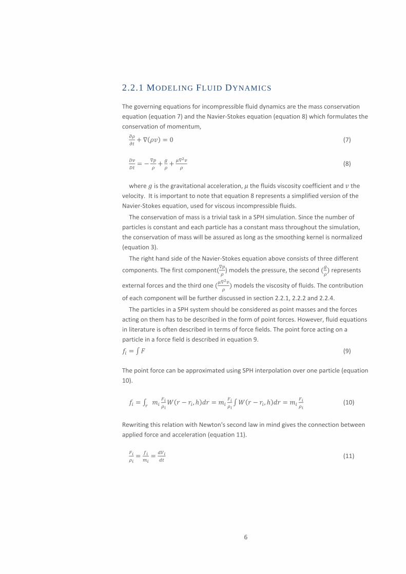
2.2.1 MODELING FLUID DYNAMICS
The governing equations for incompressible fluid dynamics are the mass conservation
equation (equation 7) and the Navier‐Stokes equation (equation 8) which formulates the
co e mentum, ns rvation of mo
0 (7)
(8)
where is the gravitational acceleration, the fluids viscosity coefficient and the
velocity. It is important to note that equation 8 represents a simplified version of the
Navier‐Stokes equation, used for viscous incompressible fluids.
The conservation of mass is a trivial task in a SPH simulation. Since the number of
particles is constant and each particle has a constant mass throughout the simulation,
the conservation of mass will be assured as long as the smoothing kernel is normalized
(equation 3).
The right hand side of the Navier‐Stokes equation above consists of three different
components. The first component ) models the pressure, the second represents
external forces and the third one models the viscosity of fluids. The contribution
of each component will be further discussed in section 2.2.1, 2.2.2 and 2.2.4.
The particles in a SPH system should be considered as point masses and the forces
acting on them has to be described in the form of point forces. However, fluid equations
in literature is often described in terms of force fields. The point force acting on a
a force field is described in equation 9. particle in
(9)
The point force can be approximated using SPH interpolation over one particle (equation
10).
, , (10)
Rewriting this relation with Newton's second law in mind gives the connection between
applied force and acceleration (equation 11).
(11)
6
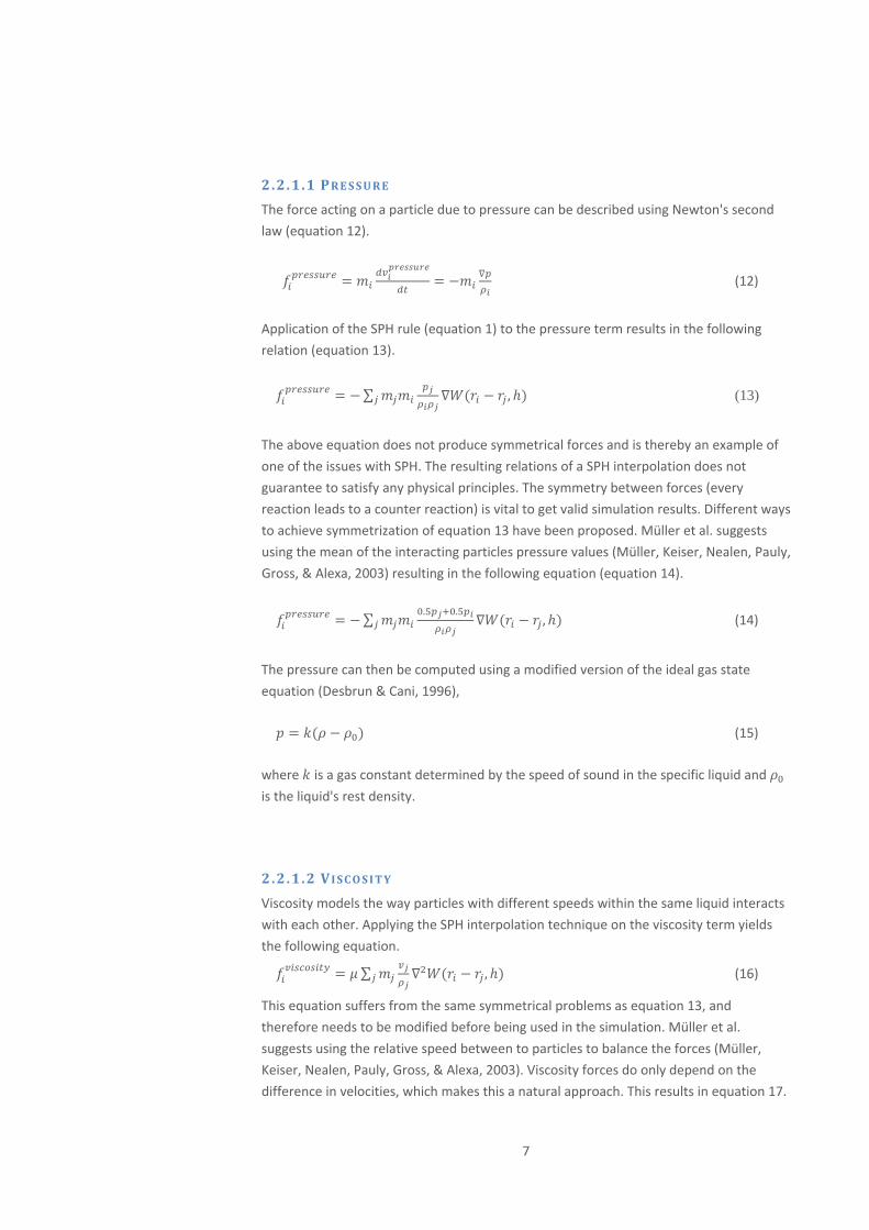
2.2.1.1 PRESSURE
The force acting on a particle due to pressure can be described using Newton's second
law (equation 12).
(12)
Application of the SPH rule (equation 1) to the pressure term results in the following
relation (equation 13).
∑ , (13)
The above equation does not produce symmetrical forces and is thereby an example of
one of the issues with SPH. The resulting relations of a SPH interpolation does not
guarantee to satisfy any physical principles. The symmetry between forces (every
reaction leads to a counter reaction) is vital to get valid simulation results. Different ways
to achieve symmetrization of equation 13 have been proposed. Müller et al. suggests
using the mean of the interacting particles pressure values (Müller, Keiser, Nealen, Pauly,
Gross, & Alexa, 2003) resulting in the following equation (equation 14).
∑ . ., (14)
The pressure can then be computed using a modified version of the ideal gas state
equation (Desbrun & Cani, 1996),
(15)
where is a gas constant determined by the speed of sound in the specific liquid and
is the liquid's rest density.
2.2.1.2 VISCOSITY
Viscosity models the way particles with different speeds within the same liquid interacts
with each other. Applying the SPH interpolation technique on the viscosity term yields
th .e following equation
∑ , (16)
This equation suffers from the same symmetrical problems as equation 13, and
therefore needs to be modified before being used in the simulation. Müller et al.
suggests using the relative speed between to particles to balance the forces (Müller,
Keiser, Nealen, Pauly, Gross, & Alexa, 2003). Viscosity forces do only depend on the
difference in velocities, which makes this a natural approach. This results in equation 17.
7
∑ , (17)
Clavet et al. presents a different approach, applying radial pairwise impulses, to model
viscosity (Clavet, Beaudoin, & Poulin, 2005). The size of the impulses depends on the two
pa rds each other (equation 18 and 19). rticles speed towa
· ̂ (18)
(19)
and are coefficients used to control the viscosity’s linear and quadratic
dependencies on velocity. Impulses are only applied if is greater than 0, the proposed
algorithm will therefore only cause forces when particles are moving towards each
other.
2.2.1.3 SURFACE TENSION
The Navier‐Stokes model does not include forces due to surface tension. This is therefore
often added as a separate part. Surface tension can be seen as a force striving to
minimize curvature by applying forces towards the core of the liquid in the direction of
the surface normal. The more curved a surface is, the greater surface tension force will
be generated.
Morris proposes the use of a color field to determine forces acting upon a set of
particles to su Morris, 2000). The color field is defined as, due rface tension (
∑ , . (20)
This is simply a measure of the particle distribution. The surface normal field of a set of
pa s as the gradient of the color field (equation 21). rticle is defined
(21)
The curva
| |
ture of a surface can be calculated as,
. (22)
The forc due to surface tension ae c n then be calculated using the following equation.
| | (23)
Where is a scalar coefficient used to scale the amount of surface tension to be applied.
The magnitude of the normal can be used to restrict the surface tension to only be
applied to parts of the liquid close to a surface.
2.2.1.4 EXTERNAL FORCES
External forces such as gravity and collision forces can be applied directly to the
particles, without the use of any interpolation technique. See chapter 3.6 for a detailed
description of the implemented collision handling algorithm.
8

9
2.2.2 SMOOTHING KERNELS
The outcome of a simulation in terms of accuracy, speed and stability is greatly affected
by the choice of smoothing kernels. As discussed earlier (see section 2.1) it is necessary
to choose kernels that are even (equation 2) and normalized (equation 3), to be able to
limit the interpolation error. In order to obtain stability it is crucial to pick smoothing
kernels that are zero with vanishing derivates at its boundaries (Müller, Keiser, Nealen,
Pauly, Gross, & Alexa, 2003).
Apart from these basic constraints it is important to consider computational time
when designing a kernel. The kernel has to be evaluated several times for each particle
in the simulation at every iteration. Even a small change in the complexity of the kernel
can have devastating effects on the simulations performance.
There are several different smoothing kernels suggested in literature, designed to
achieve different results in terms of speed and particle behavior. The most common
approach is to use different kernel types depending on the scalar component to be
interpolated. Müller et al. suggests the following set of kernels.
, 0 0
(24)
This kernel has a big computational advantage. It is relatively simple in its form and the
fact that the distance variable r only appears squared, has the advantage that the kernel
can be evaluated without computing any square roots. Which is necessecary when
calculating the distance between two particles. Müller et al. uses this kernel for density
computations.
Since the above kernel (equation 24) has vanishing gradients close to its center it is not
usefull to calculate pressure forces. The magnitudes of the forces due to pressure are
stictly dependent on the smoothing kernels gradient (equation 13) hence would the
above kernel lead to vanishing forces between particles close to each other. This is an
unwanted behaviour that tend to cause clustering of particles. The following kernel
(equation 25) was designed to address this problem and create strong repelling forces
between particles close to each other.
, 0 0
(25)
As mentioned earlier, Müller et al. uses the Laplacian to calculate forces due to viscosity
(equation 13). A negative Laplacian would cause the viscosity to increase the difference
in velocities rather than smoothen out the velocity field. Since both of the above kernels
have negative Laplacian values at some points within theire cut‐off radus, a third kernel
th an ex y s (equation 26). wi lusivl positive Laplacian i presented
, 1 0 0
(26)

2.3 COMPUTE UNIFIED DEVICE ARCHITECTURE (CUDA) CUDA, or Computer Unified Device Architecture, is NVIDIAS software and hardware
architecture for general‐purpose programming on the GPU. CUDA was released in 2007
with the purpose of making the parallel processing capabilities of the GPU accessible
through an API not related to graphics. A CUDA compatible GPU can be considered a as a
device providing a set of parallel co‐processing units to the main CPU, the host. From this
point on the GPU will be referred to as the device and the CPU as the host.
2.3.1 NVIDIA’S HARDWARE ARCHITECTURE It is necessary to have a basic understanding of NVIDIA’s hardware architecture in order
to fully utilize a CUDA compatible GPU's processing power.
CUDA enabled GPU's consists of a number of unified general‐purposed processing
units referred to as streaming multiprocessors. Each streaming multiprocessors consists
of a number of streaming processors. The multiprocessors utilizes a single instruction
multiple data (SIMD) architecture, meaning that each streaming processor, at a given
point in time, perform the exact same instructions but on different sets of data.
2.3.1.1 EXECUTION MODEL A function executed on the device is called a kernel. The same kernel is executed on the
device's all streaming multiprocessors. Each kernel executes over a grid of blocks, where
each block consists of a number of threads. It is up to the user to define the dimensions
of the grid and the blocks.
F IGURE 1 . Illustrates the CUDA execution model. Each kernel is executed over a two‐dimensional grid of
blocks. A block consists of threads organized in up to three dimensions.
Threads within the same block have access to the same shared memory (see section
2.2.1.2) and can be synchronized through a barrier‐like construct. It is however not
possible to synchronize threads executed in different blocks. The only way to achieve
synchronization over all threads is to split the workload into two separate kernels for
sequential execution. As mentioned earlier, the threads are executed in a SIMD manner.
The grid and block organization is typically used to determine which data to operate on.
10

All these facts makes the grid and block configuration a crucial part of most CUDA
implementations.
When a kernel is executed, the blocks within the kernel are distributed over the
available streaming multiprocessors. The threads within a block are then divided into
groups of 32, called warps. Threads contained by a warp are then distributed over the
streaming processors and executed in parallel. At any point in time the hardware
executes instructions from one selected warp.
2.3.1.2 MEMORY HIERARCHY
There are several different types of memory available on the device, each with different
properties such as accessibility and functionality.
Device memory (VRAM) is the counterpart of the Random Access Memory (RAM)
available on the CPU and is divided into, global memory, constant memory, texture
memory and local memory.
The global memory is the only memory type that gives full access (read/write) to both
the device and the host. It is therefore the only way to handle data transactions from the
device to the host. However, the global memory is not cached, which makes the access
times relatively high. It is therefore desirable to minimize transactions to and from this
memory type.
Both the texture and the constant memory are cached, which substantially reduces
the access times in situations where the same memory is accessed several times. In
addition, the texture memory provides hardware support for certain functions such as
interpolation etc.
The local memory has the same performance capabilities as the global memory with
the difference that it is only accessible from the specific thread that wrote to it. Since it is
slow it should be avoided and can often be substituted with the multiprocessors local
memory (on‐chip memory).
There are two types of on‐chip memory, shared memory and registers. They both have
extremely fast access times. Shared memory is shared between blocks on the same
streaming multiprocessors. It is often used as manually controlled cache, where data
from the global memory can be copied when accessed frequently within the same block
(see section 2.3.3.1). Registers are used for local storage of data which is only accessible
from a specific thread. The downside however is that each streaming multiprocessors
only have a very limited amount of on‐chip memory. If it is used without care and
consideration it might greatly affect the computational performance of an
implementation and possibly even prevent an application from executing.
11
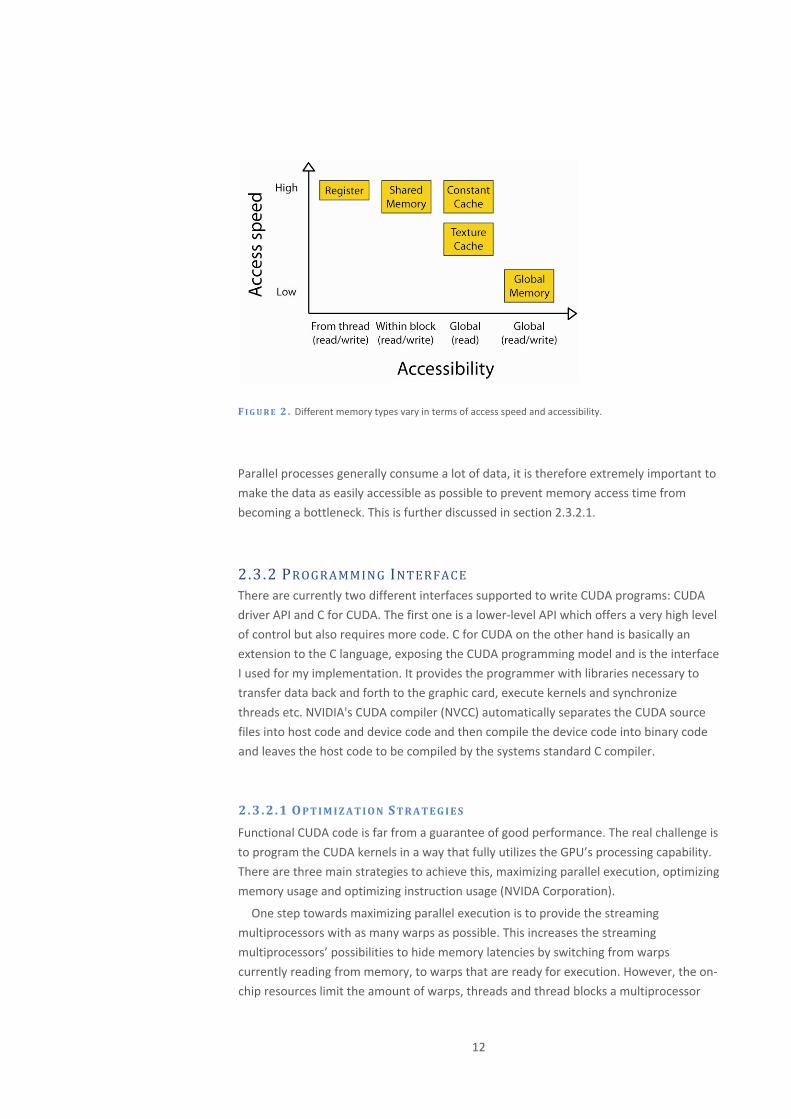
F IGURE 2 . Different memory types vary in terms of access speed and accessibility.
Parallel processes generally consume a lot of data, it is therefore extremely important to
make the data as easily accessible as possible to prevent memory access time from
becoming a bottleneck. This is further discussed in section 2.3.2.1.
2.3.2 PROGRAMMING INTERFACE There are currently two different interfaces supported to write CUDA programs: CUDA
driver API and C for CUDA. The first one is a lower‐level API which offers a very high level
of control but also requires more code. C for CUDA on the other hand is basically an
extension to the C language, exposing the CUDA programming model and is the interface
I used for my implementation. It provides the programmer with libraries necessary to
transfer data back and forth to the graphic card, execute kernels and synchronize
threads etc. NVIDIA's CUDA compiler (NVCC) automatically separates the CUDA source
files into host code and device code and then compile the device code into binary code
and leaves the host code to be compiled by the systems standard C compiler.
2.3.2.1 OPTIMIZATION STRATEGIES
Functional CUDA code is far from a guarantee of good performance. The real challenge is
to program the CUDA kernels in a way that fully utilizes the GPU’s processing capability.
There are three main strategies to achieve this, maximizing parallel execution, optimizing
memory usage and optimizing instruction usage (NVIDA Corporation).
One step towards maximizing parallel execution is to provide the streaming
multiprocessors with as many warps as possible. This increases the streaming
multiprocessors’ possibilities to hide memory latencies by switching from warps
currently reading from memory, to warps that are ready for execution. However, the on‐
chip resources limit the amount of warps, threads and thread blocks a multiprocessor
12

can handle simultaneously. The on‐chip resources available on the GeForce‐8 series is
summarized below.
• Max 24 warps per multiprocessor
• Max 768 threads per multiprocessor
• Max 28 thread blocks per multiprocessor
• Max 8192 32‐bit registers per multiprocessor
• Max 16384 bytes shared memory per multiprocessor
These resources do vary slightly depending on the graphic card available in the machine.
However, all card specific figures presented in this report are reflecting the Geforce‐8
series resource specifications, since that was the card type available at Sony Pictures
Imageworks during my internship. The ratio of active warps to the maximum number of
warps available on the GPU is called the occupancy. Higher occupancy will not
necessarily lead to better performance but it will prevent bottlenecks due to long
memory access times.
Memory access times can be reduced by avoiding data transfers to memories with low
bandwidth. Transfers between host and device units should be avoided and transfers
between global and local device memory should be minimized. One way of minimizing
threads access to the global memory is to let threads within a block load parts of the
global memory into the shared memory. This does however require that threads within
the same block needs access to data at the same place in the global memory. Another
strategy to reduce global memory access is simply to recalculate data rather than fetch
the result from previous a calculation that has been stored in the memory. Moreover, it
is possible to reduce access time by optimizing memory access patterns. It is for example
faster to fetch data that is organized in a sequential order than data that is scattered all
over the memory. Since data required for a specific warp is fetched from the memory at
the same time, a lot can be gained from making sure that the threads within that warp
will require memory that is organized sequentially in memory. Another notable fact
about the device is that it is optimized to fetch data that is organized in groups of four
(traditionally red/green/blue/alpha). Depending a little on what the access patterns look
like it is often more efficient to organize and fetch data in groups of four even if one of
the data spots is not used.
As for optimizing instruction usage, some computational heavy arithmetic functions
can be replaced with less expensive versions especially modified to perform well on the
device. This does however mean some loss of precision and should only be done in cases
where it will not affect the quality of the end result.
All these optimization techniques are discussed in more depth in NVIDIA’s CUDA
programming guide (NVIDA Corporation).
13
CHAPTER 3
IMPLEMENTATION
Knowing the advantages and weaknesses of the GPU, it is possible to implement the
algorithm in a way that will result in maximum possible utilization of the available
processing resources. Even though the SPH algorithm is the driving element behind the
whole implementation there are several important parts necessary to set up and control
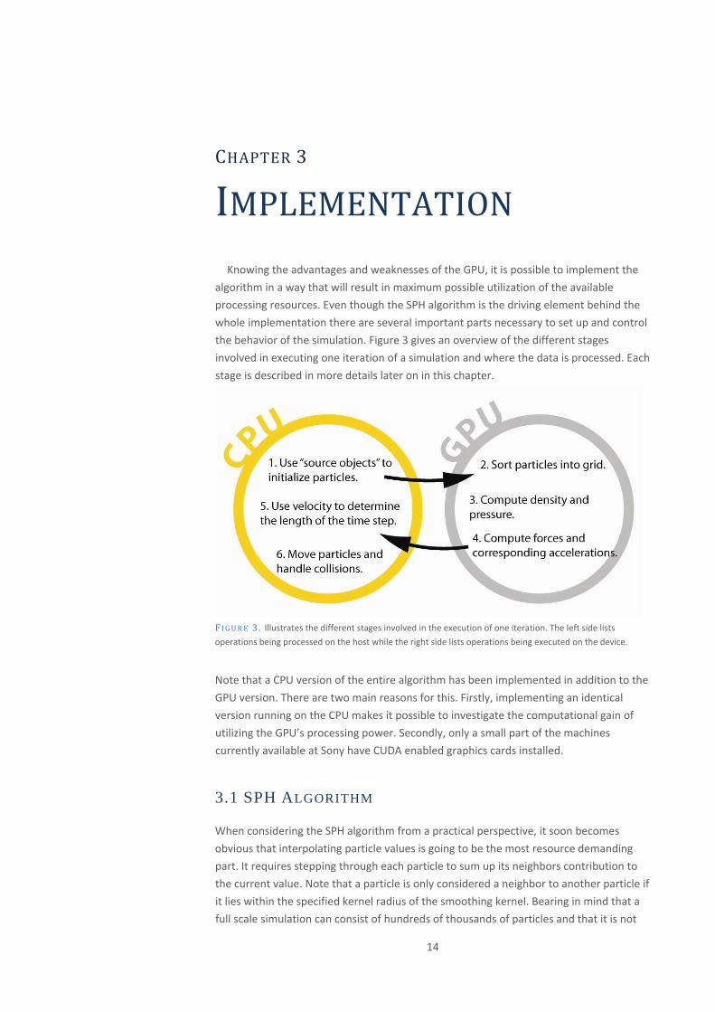
the behavior of the simulation. Figure 3 gives an overview of the different stages
involved in executing one iteration of a simulation and where the data is processed. Each
stage is described in more details later on in this chapter.
F IGURE 3 . Illustrates the different stages involved in the execution of one iteration. The left side lists operations being processed on the host while the right side lists operations being executed on the device.
Note that a CPU version of the entire algorithm has been implemented in addition to the
GPU version. There are two main reasons for this. Firstly, implementing an identical
version running on the CPU makes it possible to investigate the computational gain of
utilizing the GPU’s processing power. Secondly, only a small part of the machines
currently available at Sony have CUDA enabled graphics cards installed.
3.1 SPH ALGORITHM
When considering the SPH algorithm from a practical perspective, it soon becomes
obvious that interpolating particle values is going to be the most resource demanding
part. It requires stepping through each particle to sum up its neighbors contribution to
the current value. Note that a particle is only considered a neighbor to another particle if
it lies within the specified kernel radius of the smoothing kernel. Bearing in mind that a
full scale simulation can consist of hundreds of thousands of particles and that it is not
14
unusual that particles have around 20‐50 neighbors, a lot can be gained by speeding up
this process. Firstly, it will be necessary to find a data structure capable of quickly find a
particle’s neighbors. Secondly, the workload coupled to the interpolation has to be
processed in a way that fully utilizes the GPU’s capacity.
3.1.1 DATA STRUCTURE As discussed earlier, the nature of the SPH algorithm makes it crucial to efficiently find a
particle’s neighbors within the kernel radius. To exhaustively search through and
compare every particle in the set is a waste of resources and practically unthinkable for
anything else than extremely small particle sets. It is therefore necessary to sort the
particles into some kind of data structure that can be used to limit or guide the search
algorithm through the particle set. There are numerous different approaches to do this,
where Kd‐trees and different hash tables are examples of possible solutions. However, I
choose to sort the particles, based on position, into a uniform and wrapped grid
structure and then limit the search for particles within the kernel radius to the
corresponding and neighboring grids. By choosing a cell size equal to the kernel radius,
no points are neglected. The size and dimension of the grid is static throughout the
s each point is hashed into the grid using a simple hashing function: imulation but
% (27)
% (28)
% (29)
(30)
The above described structure makes it possible to sort an infinitely large geometric span
into the grid without changing its dimensions. Even though the hashing leads to distance
comparisons between particles that are potentially far away from each other this has
turned out to be negligible considering the computational time.
When a hashing key have been calculated for each particle, the particles are being
sorted and the position array will be reordered based on grid id. This means that
particles hashed into the same cell will be placed next to each other in the position array.
This grids structure is represented by a set of arrays. One array storing the position of
each particle, sorted in order of their hash keys and two arrays used to store the
beginning and end of each cell.
15
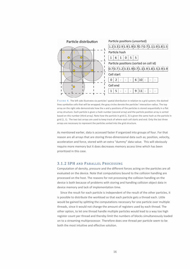
F IGURE 4 . The left side illustrates six particles’ spatial distribution in relation to a grid system; the dashed
lines symbolize cells that will be wrapped; the gray circles denote the particles’ interaction radius. The top
array on the right side demonstrate how the x and y positions of the particles is stored sequentially in a flat
array structure. Each particle is given a hash number (second array) and the particle position array is sorted
based on this number (third array). Note how the particle in grid (1, 3) is given the same hash as the particle in
grid (1, 1). The two last arrays are used to keep track of where each cell starts and end. Only the last three
arrays are necessary to represent the particles sorted into the grid structure.
As mentioned earlier, data is accessed faster if organized into groups of four. For that
reason are all arrays that are storing three‐dimensional data such as; position, velocity,
acceleration and force, stored with an extra “dummy” data value. This will obviously
require more memory but it does decreases memory access time which has been
prioritized in this case.
3.1.2 SPH AND PARALLEL PROCESSING Computation of density, pressure and the different forces acting on the particles are all
evaluated on the device. Note that computations bound to the collision handling are
processed on the host. The reasons for not processing the collision handling on the
device is both because of problems with storing and handling collision object data in
device memory and lack of implementation time.
Since the result for each particle is independent of the result of the other particles, it
is possible to distribute the workload so that each particle gets a thread each. Little
would be gained by splitting the computations necessary for one particle over multiple
threads, since it would not change the amount of registers used by each thread. The
other option, to let one thread handle multiple particles would lead to a way too high
register count per thread and thereby limit the numbers of blocks simultaneously loaded
on to a streaming multiprocessor. Therefore does one thread per particle seem to be
both the most intuitive and effective solution.
16
3.1.2.1 GRID AND BLOCK DIMENSION
When it comes to find the most appropriate grid and block configuration it is important
to determine if there are any dependencies between threads that can be taken
advantage of. For example, if the threads can be organized into blocks where each
thread will require the same data from global memory, a lot can be gained by loading
that specific part of the global memory into the shared memory. Such a relation can be
found between particles sorted into the same cell, since they got the same potential
neighbors.
However, the amount of particles in one cell can vary greatly, some cells may be
empty or only containing a few particles where as other cells may contain hundreds or
even thousands of particles. Since the amount of threads in a block has to be static
throughout a kernel this uneven distribution makes it hard to take advantage of this
similarity by using the shared memory.
Nonetheless, a certain level of similar or even identical data dependencies can be
achieved by sorting the particle array on cell index and then divide the array into equally
big chunks and distribute them over the blocks. Some block will contain particles from
several different cells with rather different data dependencies while as other blocks will
contain particles from only on cell with very similar data dependencies. Even if this
would not make it possible to utilize the shared memory it will at least lead to better
coherence in the memory reads. In addition, this brings up the possibility to make use of
the texture memory. Since the above described setup will result in a lot of identical
memory requests close to each other (in time) it has great potential of taking advantage
of the texture memory’s ability to cache data. Accessing data in the cached memory is
nearly as fast as to read from on‐chip memory. By binding the global memory arrays to
textures and use texture lookups to fetch data the memory access time is improved
drastically.
The conclusion is that since we cannot find a way to predict the spatial limits of
particles sorted into a specific block, the best solution would be a flat grid and block
configuration.
3.1.2.2 OCCUPANCY
To fully take advantage of the GPUs parallel processing capability it is necessary to
maximize the amount of active threads on each multiprocessor. As discussed in section
2.3.3.2 the on‐chip resources limits the amount of threads a multiprocessor can handle
simultaneously. The most limiting factor in this implementation turned out to be the
number of registers possible to load on to a multiprocessor. The original kernel used to
interpolate the forces acting on the particles each thread consumed 28 registers. With
that amount of registers per thread and 64 threads per block the streaming
multiprocessor would only be able to handle 8 warps simultaneously out of the
maximum of 24 active warps. This leads to an occupancy value of 33%. Such a low
occupancy value will leave the streaming processors with few warps to choose between
hence it poses a major risk to cause memory access times to limit the CPU’s
performance. By moving the least accessed data from the register to the private global
17
memory and thereby decreasing the register use from 28 to 20 the occupancy value can
be increased to 50%. Note that such a change can potentially harm the performance of a
kernel since it will increase the access time to the data moved to the global memory. To
fully predict the outcome of such a change is almost impossible. Extensive testing and
clocking of processing times has proven that this change led to significant speedups.
3.1.2.3 KERNELS
Since the different forces acting on a particle all depends on density and it is not possible
to synchronize threads across a kernel, it is necessary to first execute the density
computations in a separate kernel. This is the only way to guarantee that the density for
all particles have been evaluated before proceeding to calculate forces. The same type of
division into separate kernels is necessary to guarantee that all particles have been
sorted into the grid before computing density. The process order can be summaries as,
1. Load particle position and velocity arrays on to the device.
2. Execute kernel to sort particles into grid structure.
3. Execute kernel to compute density.
4. Execute kernel to compute forces and corresponding accelerations.
5. Load acceleration array from device to host.
3.1.2.4 MEMORY RESTRICTIONS
Independent of what graphics card available there will always be a restriction in how
much data that can be loaded onto the device. It will thereby limit the amount of
particles that can be processed in a single kernel call. One way to handle this issue, is to
split the work load into different kernels and execute them separately. Finding an
appropriate way to split the work load is not trivial. It is necessary to find a way to evenly
distribute the work load amongst multiple kernels and still limit and keep track of each
kernel’s data dependencies.
In our case, we do have a clear spatial restriction of data dependencies. If the grid
structure is divided into coherent chunks of cells the particles inside each chunk will only
require particle data from either inside the same division or cells on the outer border of
the division. However, the uneven distribution of particles complicates process of
splitting a set of particles into even chunks. One approach would be to start with one cell
and its neighboring cells and then step by step start to expand the set of included cells,
continually checking so that the included particles do not exceed the maximum amount
that can be loaded onto the device. There are however some issues with such an
approach. Firstly, particle sets with particles distributed over a very limited set of cells
will require copying the same particle data to more than two different kernels and can
be seen as a waste of resources. It is theoretical possible that the particle count within a
cell and its neighbors exceeds the device’s particle limit. Secondly, there is no guarantee,
not even probable that such an approach would be able to find the optimal split. As a
18
consequent there is a risk of using more kernels than possible and that would greatly
harm the performance of the algorithm.
It is probably possible to modify and fine tune the above described algorithm to find
solutions to these problems. However, my implementation does not support splitting
work load between kernels and the maximum amount of particles in a simulation is
thereby limited. On the specific card available at Sony the amount of particles is limited
to about 3 millions. This is a relatively high limit considering that typical simulations
rarely exceeds a couple of hundred of thousands of particles. This and the limited time
frame for this project were the main reasons for not putting more effort into resolving
this potential problem.
3.1.2 NORMALIZE DENSITY A consequence of approximating the density using equation 4 is that particles in the
outer bounds of a liquid will receive a lower density value than other particles. This is
due to the lower amounts of neighbors. It is with other words impossible to arrange a set
of particles in a structure resulting in uniform density. This results in that the pressure
force continuously try to compensate for the difference in density by pushing particles
on the surface towards the core of the liquid, preventing the liquid to reach a rest state.
One way of compensating for the lower density values near the surface is to use a
“normalized” value which is calculated using the neighboring particles density values
quat n 31). (e io
∑ , (31)
This is evening out the density in areas where the density is changing rapidly and
compensates for the low density of particles near the surface. However, normalizing the
density field requires an additional loop through all the particles and will thereby lead to
a considerable amount of additional computations. It is therefore implemented as an
option to be considered in cases where problems due to an uneven density field are
experienced.
3.1.3 SMOOTHING KERNELS Choosing an appropriate set of smoothing kernels is crucial for the outcome of the
simulation. A badly choose set of kernels will harm the performance of the simulation.
Not only in terms of computational time but more importantly it may cause
inappropriate particle behavior.
I have experimented with multiple kernel sets, both sets proposed in the literature
(Clavet, Beaudoin, & Poulin, 2005) and own suggestions. However, best performance
was achieved with the set proposed by Müller et al., described in section 2.2.5, hence
they are the kernels used in the final implementation.
19

3.2 INTEGRATION METHOD The integration step is what drives the simulation forward by integrating the particles
attributes (position and velocity) to move the particles through space. The discontinuous
and non‐linear nature of most computer simulations make it impossible to find an exact
solution to differential equation of this sort. There are however several methods that
can be used to find approximate solutions.
The Euler method simply updates the particles velocities using the result of the
applied forces, and then uses the velocity to move the particles to a new position. The
simplicity and intuitive approach of Euler has made it a commonly used integration
method. However, the error arising from the Euler method is directly proportional to the
step size which can lead to numerical instability during stiff conditions. It is therefore
often necessary to maintain higher‐order techniques to maintain stability and accuracy
throughout a simulation. Runge‐Kutta is a commonly used higher‐order integration
technique which uses a weighted average of a particles velocity at different points
between its current and next position. The higher level of stability and accuracy comes at
the cost of calculating the resulting forces/velocities at additional times.
The implemented sph‐solver supports both Euler and a fourth‐order Runge‐Kutta
method.
3.2.1 STEP SIZE The time difference between two iterations in a simulation is vital for the outcome. A too
big step size will lead to instabilities and poor accuracy, while a too short step size will
lead to an unnecessary long computation time. The challenge is to find a step size that is
just long enough to give an acceptable level of accuracy. The distance a particle is moved
between two iterations is in proportion to the accuracy of the approximation of the
particles path. Meaning that the longer distance a particle move between two time steps
the bigger will the error and instability of the simulation become. This is a common
problem encountered when explicit time‐marching schemes are used to find numerical
solutions to differential equations. Courant et al. proposed a partial solution to this
problem by using the velocity to constrain the size of the time step (Courant, Friedrichs,
& Lewy, 1928); this constraint is often referred to as the CFL‐condition.
The level of accuracy can be controlled by using the fastest moving particle to
determine the step size. In my implementation the smoothing kernels cut‐off radius is
used to limit the allowed maximum distance a particle can move during one time step.
step is calculated as The time
(32)
where is a user defined coefficient used to control the strictness of the displacement
condition. The above expression is used in combination with a user defined minimum
and maximum step size to handle certain extreme cases and to be able to limit the
maximum processing time for one iteration.
20
3.3 PARTICLE SOURCES
Particles are added to the simulations by initializing particles within the bounds of a
user‐defined source objects. These objects are represented by signed distance fields
(Bærentzen & Aanæs, 2002). Signed distance fields are discrete scalar fields were each
voxel contains the shortest distance to the surface of an object. A positive value
indicates that the voxel is outside an object and a negative value that it is located inside
an object.
The initial distance between the particles within the bounding volume determines not
only the amount of particles but also the initial behavior of the liquid. Birthing particles
close to each other (relatively to the interaction radius) will lead to a higher initial
density than adding particles with a long distance between each other. In most cases it is
desirable to initialize particles with an initial mean density close to the rest density. Such
a particle set would neither expand nor contract but simply fill up the user‐defined
volume which makes it easy to handle.
Particle source objects are being passed to the solver at every frame. Particles are
being added to the simulation if there interpolated distance value is negative and they
are on a user‐specified distance from any other particle in the simulation. The particles
are uniformly distributed within the defined source object and organized in a tetrahedral
pattern. There initial velocities are set according to a separate vector field passed in
together with the distance field.
3.4 COLLISION DETECTION Objects in the particles environment will interact with and restrict particle’s movement
in different ways. Such objects will further on be referred to as collision objects. This
interaction between particles and external objects has to be handled in an effective yet
reasonable accurate manner. It does not only require a suitable collision handling
algorithm but also a way to represent the collision objects in a precise and efficient
manner.
3.4.1 COLLISION OBJECTS Collision objects are represented by a signed distance field and a velocity field, just like
the particle source objects described in section 3.4. The surface normal is approximated
and stored in a separate field by calculating the gradient of the distance field. The
velocity field will be searched through to determine if the collision object contains any
moving points at the current iteration or if it can be flagged as a static object.
3.4.1.1 ADVECTION OF COLLISION OBJECTS
Collision object are passed to the simulation at every frame and the solver might be
forced to run substeps to acquire stability (see section 3.31). This leads to an
21

unacceptable discontinuity in the collision object representation. However, the
corresponding velocity field can be used to approximate a collision objects position at a
specific substep. The basic idea is to use the velocity field to track the movement of the
distance field values. This is a very similar approach to the technique Doyub et al.
purposed to use to acquire Eulerian motion blur (Doyub & Hyeong‐Seok, 2007). This is a
relatively expensive operation, especially if a large number of substeps are required, but
algorithms of similar sort have due to their isolated and repetitive manner been proven
suitable for being processed on the GPU (Fridlund, 2009). Fridlund’s implementation was
available at Sony Pictures Imageworks and has been used as a base to track the collision
objects between frames.
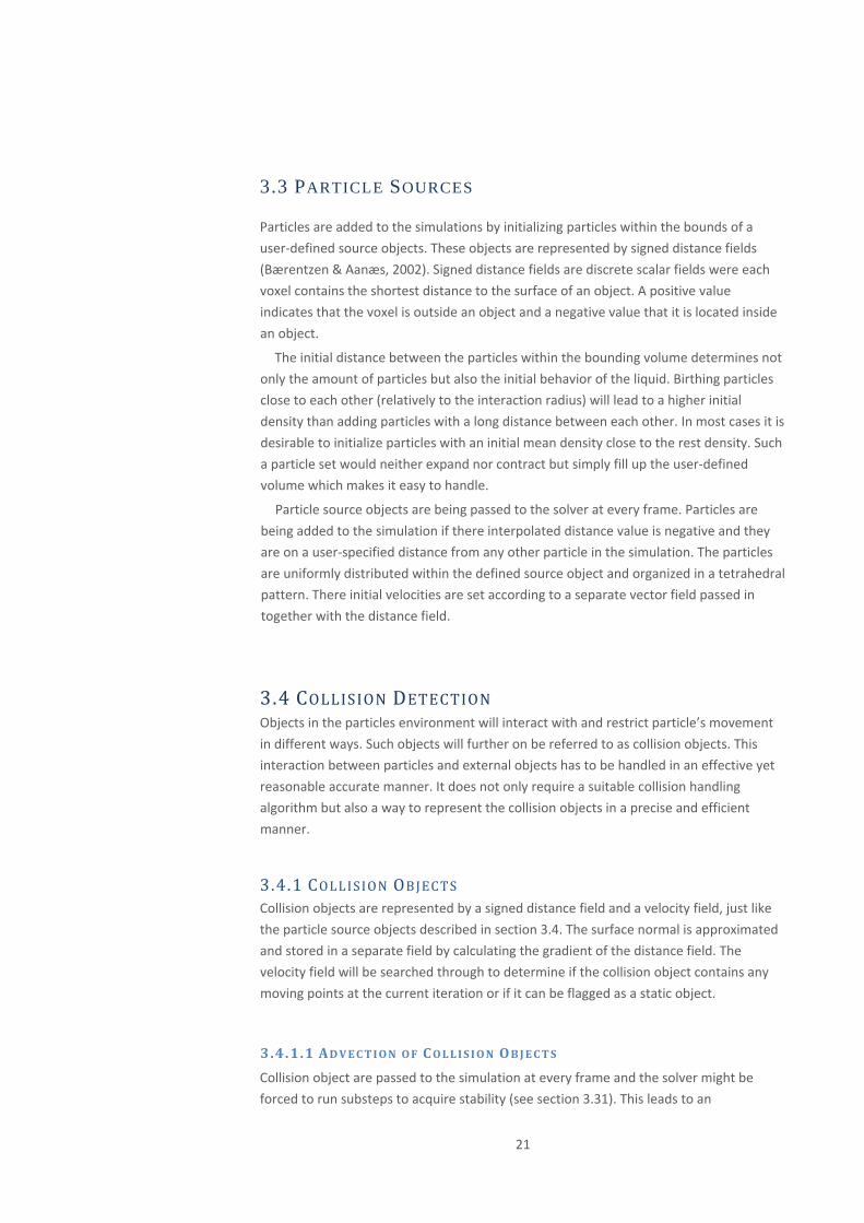
3.4.2 COLLISION ALGORITHM All particles are checked for possible collision at every iteration. This is done by first
controlling if the particle's new position ( ) is within the bounds of any
collision object and if so, it's distance value is interpolated from the distance field. If the
value is negative a collision has occurred.
There are basically two different reasons for collision. A particle moves into an object
or an object moves into a particle. The main different when handling the two cases is
that if a particle moves into an object the point of collision can be calculated using linear
interpolation,
(33)
where is the particle’s new position, and the distance from the collision object
to and respectively and the velocity of the particle.
Determining the point of impact is harder if the object moves into the particle.
However, in that case the particle can be pushed out of the collision object by using the
gradient and the point on the surface where the particle surfaces can be used as the
collision point. When the point of impact have been determined the particles velocity
are divided into two components, velocity in the direction of the surface normal ( ) and
ng the tangent of the object ( ), velocity alo
(34) ·
. (35)
ped and reflected. The is dam
(36)
Fr ti is modeled b
· · (37)
ic on y applying an opposing force acting over time to ,
If the velocity of the collision object (along its surface normal) is greater than then
is set to match the collision object's velocity.
The particle is then moved the distance between to in the direction of its newly
calculated and . Figure 5 illustrates the involved parameters relations.
22
F IGURE 5 . Illustrates the different values involved in the collision handling algorithm.
23

CHAPTER 4
RESULTS This chapter will focus on the results of the previously described implementation. The
result can both be judged by how well the particles behavior manage to represent a
fluid, and how efficient the implementation is computational wise.
4.1 PARTICLE BEHAVIOR One of the most challenging parts of achieving good particle behavior has been to
scale the forces between particles. If the force is too strong it will create a hyperactive
particle behavior and prolong the simulation time by increasing the amount of iterations.
On the other hand, a too week force would not be able to maintain the distance
between particles. This becomes extra obvious when a strong gravitation force is acting
upon the particles and pushing them towards a collision object. If the force is too week
the particles will be pressed flat onto the object while a too strong force would cause an
“explosion” of particles. It is important to find a balance. A force strong enough to
prevent the gravitation to compress the liquid and yet not overcompensating for
particles that are too close to each other.
The implemented algorithm manages to produce particle sets that well represent
basic fluid behavior. Figure 6 shows the result of a simulation of a liquid first being
poured into a cup and poured from the cup onto a ground plane. Approximately 300,000
particles were used in the simulation and it took about 12 seconds per frame to process
it.
F IGURE 6 . Illustrates the result of a simulation involving about 300, 000 particles organized in time order,
from left to right and top to bottom. The particles have been transformed into a polygon surface before being
lightened and rendered.
24
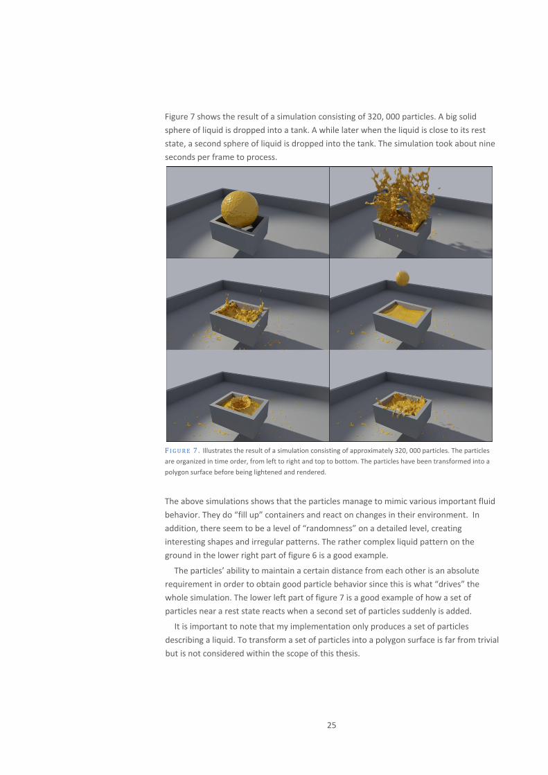
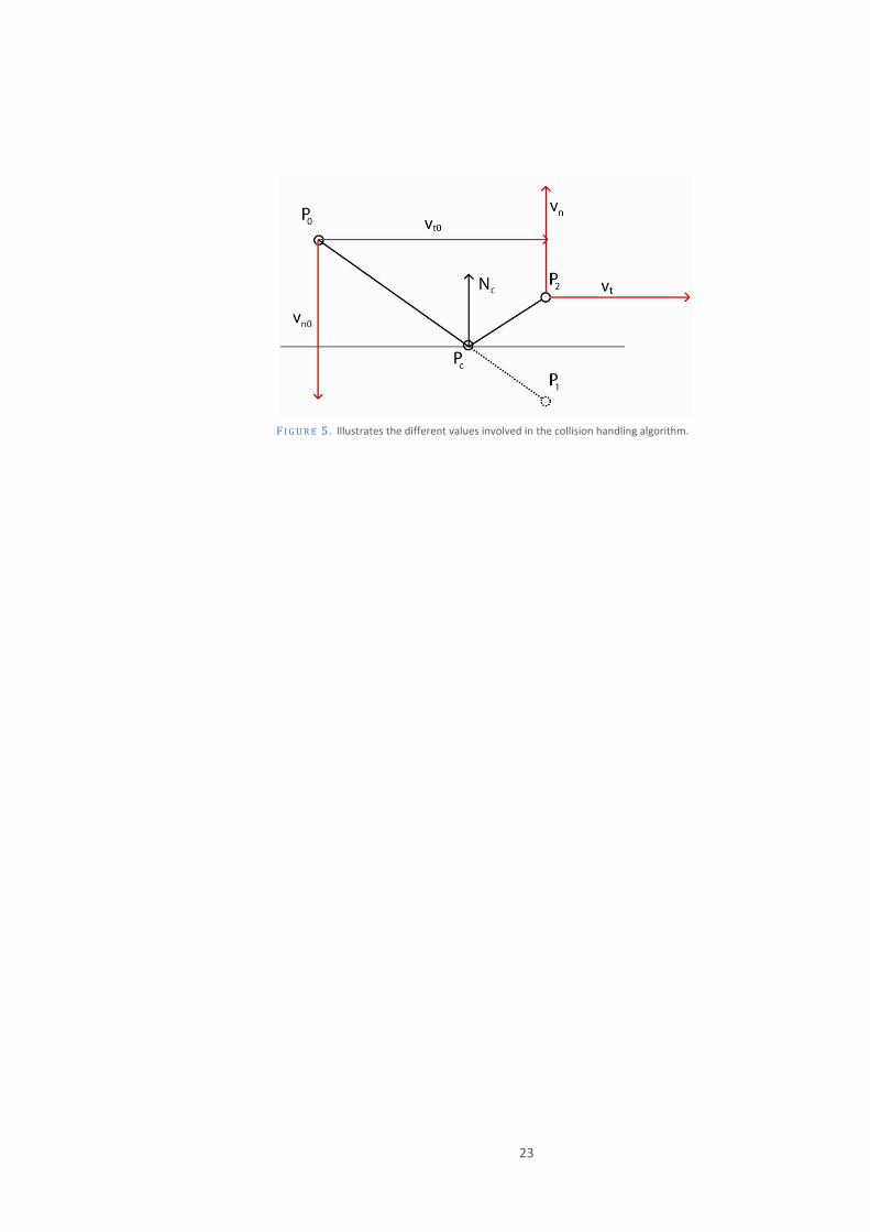
Figure 7 shows the result of a simulation consisting of 320, 000 particles. A big solid
sphere of liquid is dropped into a tank. A while later when the liquid is close to its rest
state, a second sphere of liquid is dropped into the tank. The simulation took about nine
seconds per frame to process.
F IGURE 7 . Illustrates the result of a simulation consisting of approximately 320, 000 particles. The particles
are organized in time order, from left to right and top to bottom. The particles have been transformed into a
polygon surface before being lightened and rendered.
The above simulations shows that the particles manage to mimic various important fluid
behavior. They do “fill up” containers and react on changes in their environment. In
addition, there seem to be a level of “randomness” on a detailed level, creating
interesting shapes and irregular patterns. The rather complex liquid pattern on the
ground in the lower right part of figure 6 is a good example.
The particles’ ability to maintain a certain distance from each other is an absolute
requirement in order to obtain good particle behavior since this is what “drives” the
whole simulation. The lower left part of figure 7 is a good example of how a set of
particles near a rest state reacts when a second set of particles suddenly is added.
It is important to note that my implementation only produces a set of particles
describing a liquid. To transform a set of particles into a polygon surface is far from trivial
but is not considered within the scope of this thesis.
25
4.2 PERFORMANCE
The computational time strongly depends on several parameters: The amount of
particles, the radius of the smoothing kernel and the spatial distribution of the particles.
A CPU version of the algorithm was implemented in order to easily investigate the
performance gained by utilizing the GPU.
A benchmark test was setup to compare execution times between the two
implementations. Particles were initialized within the bounds of a sphere at an initial
mean density equal to the rest density. No gravity was applied and no collision objects
were included in the setup. Each liquid was simulated for 4 seconds (100 frames, 25
frames/second), the time value presented in figure 8 are the mean execution time per
frame. As the figure shows, the GPU accelerated algorithm is approximately 40 times
faster than the one running solely on the CPU.
F IGURE 8 . Illustrates the difference in terms of execution time when processing the simulation on the GPU
versus the CPU. The time values presented are the mean execution time per frame, based on a 100 frame long
simulation.
0,03 0,1 0,18 0,35 0,491,32
3,4
6,36
12,31
0,
5,
10,
15,
20,
25k 100k 200k 400k 600k
20,18
GPU
CPU
Number of particles
Execution tim
e (secon
ds/frame)
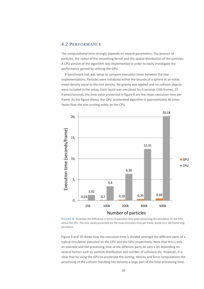
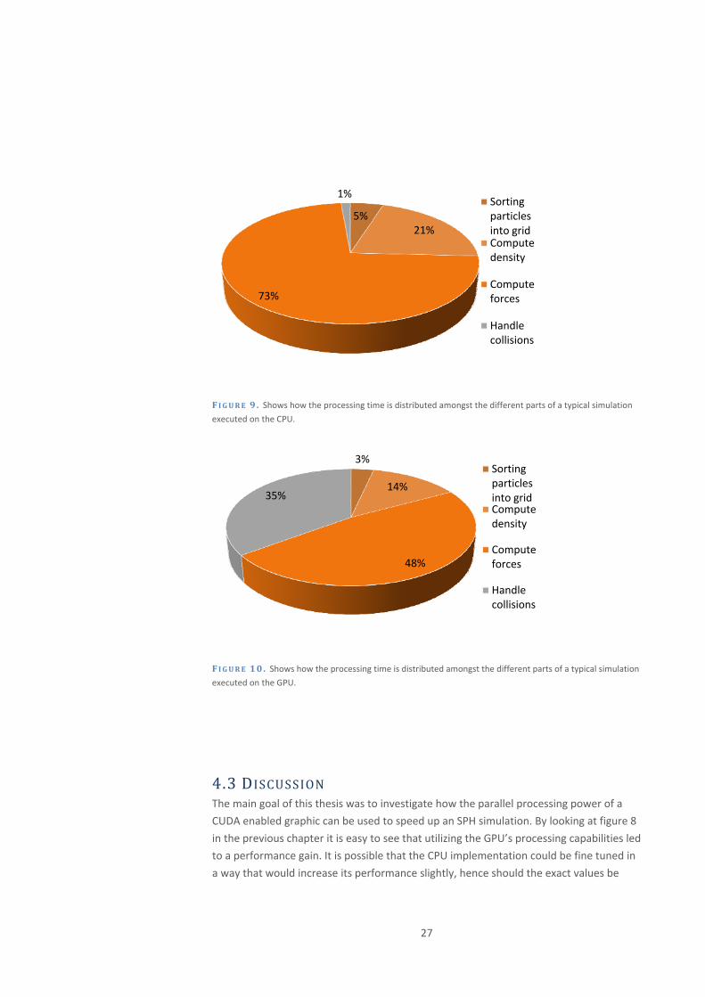
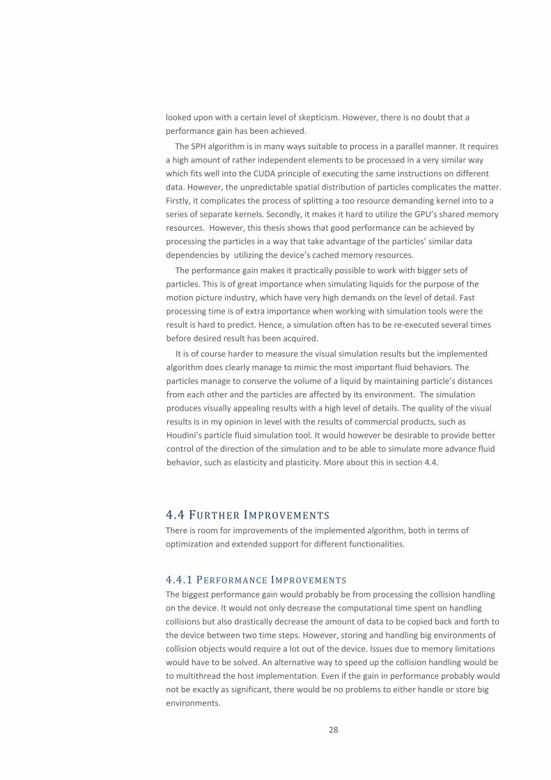
Figure 9 and 10 shows how the execution time is divided amongst the different parts of a
typical simulation executed on the CPU and the GPU respectively. Note that this is only
an example and the processing time of the different parts do vary a lot depending on
several factors such as, particle distribution and number of collisions etc. However, it is
clear that by using the GPU to accelerate the sorting, density and force computations the
processing of the collision handling has become a large part of the total processing time.
26
5%21%
73%
1%Sorting particles into gridCompute density
Compute forces
Handle collisions
F IGURE 9 . Shows how the processing time is distributed amongst the different parts of a typical simulation
executed on the CPU.
3%
14%
48%
35%
Sorting particles into gridCompute density
Compute forces
Handle collisions
F IGURE 10. Shows how the processing time is distributed amongst the different parts of a typical simulation
executed on the GPU.
4.3 DISCUSSION The main goal of this thesis was to investigate how the parallel processing power of a
CUDA enabled graphic can be used to speed up an SPH simulation. By looking at figure 8
in the previous chapter it is easy to see that utilizing the GPU’s processing capabilities led
to a performance gain. It is possible that the CPU implementation could be fine tuned in
a way that would increase its performance slightly, hence should the exact values be
27
looked upon with a certain level of skepticism. However, there is no doubt that a
performance gain has been achieved.
The SPH algorithm is in many ways suitable to process in a parallel manner. It requires
a high amount of rather independent elements to be processed in a very similar way
which fits well into the CUDA principle of executing the same instructions on different
data. However, the unpredictable spatial distribution of particles complicates the matter.
Firstly, it complicates the process of splitting a too resource demanding kernel into to a
series of separate kernels. Secondly, it makes it hard to utilize the GPU’s shared memory
resources. However, this thesis shows that good performance can be achieved by
processing the particles in a way that take advantage of the particles’ similar data
dependencies by utilizing the device’s cached memory resources.
The performance gain makes it practically possible to work with bigger sets of
particles. This is of great importance when simulating liquids for the purpose of the
motion picture industry, which have very high demands on the level of detail. Fast
processing time is of extra importance when working with simulation tools were the
result is hard to predict. Hence, a simulation often has to be re‐executed several times
before desired result has been acquired.
It is of course harder to measure the visual simulation results but the implemented
algorithm does clearly manage to mimic the most important fluid behaviors. The
particles manage to conserve the volume of a liquid by maintaining particle’s distances
from each other and the particles are affected by its environment. The simulation
produces visually appealing results with a high level of details. The quality of the visual
results is in my opinion in level with the results of commercial products, such as
Houdini’s particle fluid simulation tool. It would however be desirable to provide better
control of the direction of the simulation and to be able to simulate more advance fluid
behavior, such as elasticity and plasticity. More about this in section 4.4.
4.4 FURTHER IMPROVEMENTS There is room for improvements of the implemented algorithm, both in terms of
optimization and extended support for different functionalities.
4.4.1 PERFORMANCE IMPROVEMENTS The biggest performance gain would probably be from processing the collision handling
on the device. It would not only decrease the computational time spent on handling
collisions but also drastically decrease the amount of data to be copied back and forth to
the device between two time steps. However, storing and handling big environments of
collision objects would require a lot out of the device. Issues due to memory limitations
would have to be solved. An alternative way to speed up the collision handling would be
to multithread the host implementation. Even if the gain in performance probably would
not be exactly as significant, there would be no problems to either handle or store big
environments.
28

There is also room for improvement due to increased occupancy of the streaming
multiprocessors. As discussed in section 3.1.2.2 the occupancy of the current
implementation is 50%. If the register usage can be further reduced (without moving
data from the registers to the global memory) it is likely to experience a performance
gain. The importance of such a change is hard to predict since it depends on how big the
current delays caused by memory access time are.
4.4.2 FUNCTIONALITY The current implementation supports the necessary parameters to set up and simulate
the basic behavior of a liquid. However, to make an SPH simulation tool real useful in the
motion picture industry it is important to provide ways to control the outcome of a
simulation. It is important to support simulation of a wide spectrum of different types of
liquids but it is also useful to have tools to control the outcome in more explicit ways.
4.4.2.1 ELASTICITY AND PLASTICITY
A perfectly elastic fluid will remember its original rest shape and will strive to regain it
while a perfectly plastic substance always will consider the current state as its rest state.
Elastic behaviors can me simulated by adding springs between pairs of neighboring
particles and plastic behavior can be modeled by changing these springs (Clavet,
Beaudoin, & Poulin, 2005).
4.4.2.2 STICKINESS
Stickiness between particles and collision objects can be simulated by simply adding an
impulsive force, in the direction of the surface normal, to particles within a certain range
from a collision object’s surface.
4.4.2.3 SINKS
Provide the user with the possibility to remove certain particles from the simulation.
Sinks can be used to remove particles that are too far away, or for other reasons are not
important for the outcome of the simulation.
4.4.2.4 FORCE FIELDS
Force fields allow the user to add external forces to a particle set. The amount and
direction of the force to be added can be explicitly defined through a force field.
4.4.3.5 FRICTION FIELD
The current implementation only supports the use of a constant friction coefficient. A better solution would be to read the friction coefficient from a scalar field
29
coupled to each collision object. That way it would be possible to define different friction coefficients for different objects and even on different parts of an object.
4.4.3.6 SUPPORT FOR UNLIMITED NUMBER OF PARTICLES
As discussed in section 3.1.2.4, the current implementation can only handle a limited amount of particles determined by the memory available on the device. A solution to this issue would be to split the workload into multiple kernels and execute them after another.
30

CHAPTER 5
REFERENCES
Amad, T., Imura, M., Yasumoto, Y., Yamabe, Y., & Chihara, K. (2004). Particle‐based fluid
simulaton on gpu. ACM Workshop on General‐Purpose Computing on Graphics
Processors.
Bærentzen, J. A., & Aanæs, H. (2002). Computing discrete signed distance fields from
triangle meshes. Lyngby: Informatics and Mathematical Modelling, Technical University
of Denmark, DTU.
Che, S., Boyer, M., Meng, J., Tarjan, D., Sheaffer, J., & Skadron, K. (68:1370‐1380). A
performance study of general‐purpose applications on graphics processors using CUDA.
Journal of Parallel and Distributed Computing , 2008.
Clavet, S., Beaudoin, P., & Poulin, P. (2005). Particle‐based Viscoelastic Fluid Simulation.
Eurographics/ACM SIGGRAPH Symposium on Computer Animation, (ss. 219‐228).
Courant, R., Friedrichs, K., & Lewy, H. (1928). Über die partiellen Differenzengleichungen
der mathematischen Physik. Mathematische Annalen , 32‐74.
Desbrun, M., & Cani, M. P. (1996). Smoothed particles: A new paradigm for animating
highly deformable bodies. In Proceedings of EG Workshop on Computer Animation and
Simulation, (ss. 61‐76).
Doyub, K., & Hyeong‐Seok, K. (2007). Eulerian Motion Blur. ACM SIGGRAPH /
Eurographics Symposium on Computer Animation, (ss. 120‐131).
Evans, C., & Kochanek, C. (1989). The tidal disruption of a star by a massive black hole.
Astrophysical Journal, Part 2 ‐ Letters (ISSN 0004‐637X) , 346:L13‐L16.
Fridlund, A. (2009). Voxel Processing for Visual Effects. Norrköping: Linköpings
Universitet.
Gingold, R., & Monaghan, J. (1977). Smoothed particle hydrodynamics: theory and
application to non‐spherical stars. Notices of the Royal Astronomical Society , 181:375‐
389.
Harada, T., Kawaguchi, Y., & Koichiro, K. (2007). Smoothed Particle Hydrodynamics on
GPUs. Computer Graphics International.
Kessenish, J., & Baldwin, R. (u.d.). OpenGL Shading Language. Hämtat från OpenGL:
http://www.opengl.org/documentation/glsl/ den 1 Mars 2009
Kolb, A., & Cuntz, N. (2005). Dynamic Particle Coupling for GPU‐based Fluid Simulation.
Proc. Of 18th Symposium on Simulation Technique, (ss. 722‐727).
Lucy, L. (1977). A Numerical Approach to the Testing of the Fission Hypothesis.
Astronomical Journal , 82(12)1013‐1024, 1013‐1024.
Microsoft. (n.d.). DirectX 10. Retrieved Mars 1, 2009, from
http://www.microsoft.com/games/en‐US/aboutgfw/Pages/directx10‐a.aspx
31
32
Monaghan, J., & Humble, R. (1991). Arbitrary Incompressible Flow with SPH.
Monaghan, J., & Kos, A. (1999). Solitary waves on a Cretan Beach. J. Waterway, Port,
Coastal, and Ocean Engrg, ASCE , 125,3.
Morris, J. (2000). Simulating surface tension with smoothed particle hydrodynamics.
International Journal for Numerical Methods in Fluids , 33(3):333‐353.
Müller, M., Keiser, R., Nealen, A., Pauly, M., Gross, M., & Alexa, M. (2003). Particle‐based
fluid simulation for interactive applications. In Proceedings of the 2003 ACM SIGGRAPH/
Eurographics‐ Symposium on Computer Animation, (ss. 154‐159).
NVIDA Corporation. (n.d.). CUDA Zone. Retrieved June 1, 2009, from NVIDA CUDA
Programming Guide 2.0:
http://developer.download.nvidia.com/compute/cuda/2_0/docs/NVIDIA_CUDA_Progra
mming_Guide_2.0.pdf
Takeda, H., Miyama, S., & Sekiya, M. (1994). Numerical Simulation of Viscous Flow by
Smoothed Particle Hydrodynamics. Progress of Theoretical Physics , 92:939‐960.