a somewhat gentle introduction to differential graded
TRANSCRIPT

A somewhat gentle introduction to differentialgraded commutative algebra
Kristen A. Beck and Sean Sather-Wagstaff
Abstract Differential graded (DG) commutative algebra provides powerful tech-niques for proving theorems about modules over commutative rings. These notesare a somewhat colloquial introduction to these techniques. In order to providesome motivation for commutative algebraists who are wondering about the benefitsof learning and using these techniques, we present them in the context of a recentresult of Nasseh and Sather-Wagstaff. These notes were used for the course “Differ-ential Graded Commutative Algebra” that was part of the Workshop on ConnectionsBetween Algebra and Geometry at the University of Regina, May 29–June 1, 2012.
Dedicated with much respect to Tony Geramita
1 Introduction
Convention 1.1 The term “ring” is short for “commutative noetherian ring withidentity”, and “module” is short for “unital module”. Let R be a ring.
These are notes for the course “Differential Graded Commutative Algebra” thatwas part of the Workshop on Connections Between Algebra and Geometry heldat the University of Regina, May 29–June 1, 2012. They represent our attempt toprovide a small amount of (1) motivation for commutative algebraists who are won-dering about the benefits of learning and using Differential Graded (DG) techniques,and (2) actual DG techniques.
Kristen A. BeckDepartment of Mathematics, The University of Arizona, 617 N. Santa Rita Ave., P.O. Box 210089,Tucson, AZ 85721, USA, e-mail: [email protected]
Sean Sather-WagstaffSean Sather-Wagstaff, Department of Mathematics, NDSU Dept # 2750, PO Box 6050, Fargo, ND58108-6050 USA e-mail: [email protected]
1
2 Kristen A. Beck and Sean Sather-Wagstaff
DG Algebra
DG commutative algebra provides a useful framework for proving theorems aboutrings and modules, the statements of which have no reference to the DG universe.For instance, a standard theorem says the following:
Theorem 1.2 ([20, Corollary 1]) Let (R,m) → (S,n) be a flat local ring homo-morphism, that is, a ring homomorphism making S into a flat R-module such thatmS ⊆ n. Then S is Gorenstein if and only if R and S/mS are Gorenstein. Moreover,there is an equality of Bass series IS(t) = IR(t)IS/mS(t).
(See Definition 9.2 for the term “Bass series”.) Of course, the flat hypothesis isvery important here. On the other hand, the use of DG algebras allows for a slight(or vast, depending on your perspective) improvement of this:
Theorem 1.3 ([9, Theorem A]) Let (R,m)→ (S,n) be a local ring homomorphismof finite flat dimension, that is, a local ring homomorphism such that S has abounded resolution by flat R-module. Then there is a formal Laurent series Iϕ(t)with non-negative integer coefficients such that IS(t) = IR(t)Iϕ(t). In particular, if Sis Gorenstein, then so is R.
In this result, the series Iϕ(t) is the Bass series of ϕ . It is the Bass series of the“homotopy closed fibre” of ϕ (instead of the usual closed fibre S/mS of ϕ that isused in Theorem 1.2) which is the commutative DG algebra S⊗L
R R/m. In particular,when S is flat over R, this is the usual closed fibre S/mS∼= S⊗R R/m, so one recoversTheorem 1.2 as a corollary of Theorem 1.3.
Furthermore, DG algebra comes equipped with constructions that can be used toreplace your given ring with one that is nicer in some sense. To see how this works,consider the following strategy for using completions.
To prove a theorem about a given local ring R, first show that the assumptionsascend to the completion R, prove the result for the complete ring R, and showhow the conclusion for R implies the desired conclusion for R. This technique isuseful since frequently R is nicer then R. For instance, R is a homomorphic imageof a power series ring over a field or a complete discrete valuation ring, so it isuniversally catenary (whatever that means) and it has a dualizing complex (whateverthat is), while the original ring R may not have either of these properties.
When R is Cohen-Macaulay and local, a similar strategy sometimes allows one tomod out by a maximal R-regular sequence x to assume that R is artinian. The regularsequence assumption is like the flat condition for R in that it (sometimes) allows forthe transfer of hypotheses and conclusions between R and the quotient R := R/(x).The artinian hypothesis is particularly nice, for instance, when R contains a fieldbecause then R is a finite dimensional algebra over a field.
The DG universe contains a construction R that is similar R, with an advantageand a disadvantage. The advantage is that it is more flexible than R because it doesnot require the ring to be Cohen-Macaulay, and it produces a finite dimensional al-gebra over a field regardless of whether or not R contains a field. The disadvantage

DG commutative algebra 3
is that R is a DG algebra instead of just an algebra, so it is graded commutative (al-most, but not quite, commutative) and there is a bit more data to track when workingwith R. However, the advantages outweigh the disadvantages in that R allows us toprove results for arbitrary local rings that can only be proved (as we understandthings today) in special cases using R. One such result is the following:
Theorem 1.4 ([32, Theorem A]) A local ring has only finitely many semidualizingmodules up to isomorphism.
Even if you don’t know what a semidualizing module is, you can see the point.Without DG techniques, we only know how to prove this result for Cohen-Macaulayrings that contain a field; see Theorem 2.13. With DG techniques, you get the un-qualified result, which answers a question of Vasconcelos [41].
What These Notes Are
Essentially, these notes contain a sketch of the proof of Theorem 1.4; see 5.32,7.38, and 8.17 below. Along the way, we provide a big-picture view of some of thetools and techniques in DG algebra (and other areas) needed to get a basic under-standing of this proof. Also, since our motivation comes from the study of semid-ualizing modules, we provide a bit of motivation for the study of those gadgets inAppendix 9. In particular, we do not assume that the reader is familiar with thesemidualizing world.
Since these notes are based on a course, they contain many exercises; sketchesof solutions are contained in Appendix 10. They also contain a number of exam-ples and facts that are presented without proof. A diligent reader may also wish toconsider many of these as exercises.
What These Notes Are Not
These notes do not contain a great number of details about the tools and techniquesin DG algebra. There are already excellent sources available for this, particularly,the seminal works [4, 6, 10]. The interested reader is encouraged to dig into thesesources for proofs and constructions not given here. Our goal is to give some idea ofwhat the tools look like and how they get used to solve problems. (To help readersin their digging, we provide many references for properties that we use.)

4 Kristen A. Beck and Sean Sather-Wagstaff
Notation
When it is convenient, we use notation from [11, 31]. Here we specify our conven-tions for some notions that have several notations:
pdR(M): projective dimension of an R-module MidR(M): injective dimension of an R-module MlenR(M): length of an R-module MSn: the symmetric group on {1, . . . ,n}.sgn(ι): the signum of an element ι ∈ Sn.
Acknowledgements
We are grateful to the Department of Mathematics and Statistics at the Universityof Regina for its hospitality during the Workshop on Connections Between Algebraand Geometry. We are also grateful to the organizers and participants for providingsuch a stimulating environment, and to Saeed Nasseh for carefully reading partsof this manuscript. We are also thankful to the referee for valuable comments andcorrections. Sean Sather-Wagstaff was supported in part by a grant from the NSA.
2 Semidualizing Modules
This section contains background material on semidualizing modules. It also con-tains a special case of Theorem 1.4; see Theorem 2.13. Further survey material canbe found in [35, 38] and Appendix 9.
Definition 2.1 A finitely generated R-module C is semidualizing if the natural ho-mothety map χR
C : R→ HomR(C,C) given by r 7→ [c 7→ rc] is an isomorphism andExtiR(C,C) = 0 for all i > 1. A dualizing R-module is a semidualizing R-modulesuch that idR(C) < ∞. The set of isomorphism classes of semidualizing R-modulesis denoted S0(R).
Remark 2.2 The symbol S is an S, as in \mathfrak{S}.
Example 2.3 The free R-module R1 is semidualizing.
Fact 2.4 The ring R has a dualizing module if and only if it is Cohen-Macaulay anda homomorphic image of a Gorenstein ring; when these conditions are satisfied, adualizing R-module is the same as a “canonical” R-module. See Foxby [19, Theorem4.1], Reiten [34, (3) Theorem], and Sharp [40, 2.1 Theorem (i)].
Remark 2.5 To the best of our knowledge, semidualizing modules were first intro-duced by Foxby [19]. They have been rediscovered independently by several au-thors who seem to all use different terminology for them. A few examples of this,presented chronologically, are:

DG commutative algebra 5
Author(s) Terminology ContextFoxby [19] “PG-module of rank 1” commutative algebraVasconcelos [41] “spherical module” commutative algebraGolod [23] “suitable module” 1 commutative algebraWakamatsu [43] “generalized tilting module” representation theoryChristensen [14] “semidualizing module” commutative algebraMantese and Reiten [30] “Wakamatsu tilting module” representation theory
The following facts are quite useful in practice.
Fact 2.6 Assume that (R,m) is local, and let C be a semidualizing R-module. If R isGorenstein, then C ∼= R. The converse holds if C is a dualizing R-module. See [14,(8.6) Corollary].
If pdR(C)< ∞, then C ∼= R by [38, Fact 1.14]. Here is a sketch of the proof. Theisomorphism HomR(C,C) ∼= R implies that SuppR(C) = Spec(R) and AssR(C) =AssR(R). In particular, an element x ∈ m is C-regular if and only if it is R-regular.If x is R-regular, it follows that C/xC is semidualizing over R/xR. By inductionon depth(R), we conclude that depthR(C) = depth(R). The Auslander-Buchsbaumformula implies that C is projective, so it is free since R is local. Finally, the isomor-phism HomR(C,C)∼= R implies that C is free of rank 1, that is, C ∼= R.
Fact 2.7 Let ϕ : R→ S be a ring homomorphism of finite flat dimension. (For ex-ample, this is so if ϕ is flat or surjective with kernel generated by an R-regular se-quence.) If C is a semidualizing R-module, then S⊗RC is a semidualizing S-module.The converse holds when ϕ is faithfully flat or local. The functor S⊗R− induces awell-defined function S0(R)→S0(S) which is injective when ϕ is local. See [21,Theorems 4.5 and 4.9].
Exercise 2.8 Verify the conclusions of Fact 2.7 when ϕ is flat. That is, let ϕ : R→ Sbe a flat ring homomorphism. Prove that if C is a semidualizing R-module, then thebase-changed module S⊗R C is a semidualizing S-module. Prove that the converseholds when ϕ is faithfully flat, e.g., when ϕ is local.
The next lemma is for use in Theorem 2.13, which is a special case of Theo-rem 1.4. See Remark 2.10 and Question 2.11 for further perspective.
Lemma 2.9 Assume that R is local and artinian. Then there is an integer ρ depend-ing only on R such that lenR(C)6 ρ for every semidualizing R-module C.
Proof. Let k denote the residue field of R. We show that the integer ρ = lenR(R)µ0R
satisfies the conclusion where µ0R = rankk(HomR(k,R)). (This is the 0th Bass
number of R; see Definition 9.2.) Let C be a semidualizing R-module. Set β =rankk(k⊗R C) and µ = rankk(HomR(k,C)). Since R is artinian and C is finitely gen-erated, it follows that µ > 1. Also, the fact that R is local implies that there is anR-module epimorphism Rβ →C, so we have lenR(C)6 lenR(R)β . Thus, it remainsto show that β 6 µ0
R.The next sequence of isomorphisms uses adjointness and tensor cancellation:

6 Kristen A. Beck and Sean Sather-Wagstaff
kµ0R ∼= HomR(k,R)∼= HomR(k,HomR(C,C))∼= HomR(C⊗R k,C)∼= HomR(k⊗k (C⊗R k),C)∼= Homk(C⊗R k,HomR(k,C))
∼= Homk(kβ ,kµ)
∼= kβ µ .
Since µ > 1, it follows that β 6 β µ = µ0R, as desired. ut
Remark 2.10 Assume that R is local and Cohen-Macaulay. If D is dualizing for R,then there is an equality eR(D) = e(R) of Hilbert-Samuel multiplicites with respectto the maximal ideal of R. See, e.g., [11, Proposition 3.2.12.e.i and Corollary 4.7.8].It is unknown whether the same equality holds for an arbitrary semidualizing R-module. Using the “additivity formula” for multiplicities, this boils down to thefollowing. Some progress is contained in [17].
Question 2.11 Assume that R is local and artinian. For every semidualizing R-module C, must one have lenR(C) = len(R)?
While we are in the mood for questions, here is a big one. In every explicitcalculation of S0(R), the answer is “yes”; see [36, 39].
Question 2.12 Assume that R is local. Must |S0(R)| be 2n for some n ∈ N?
Next, we sketch the proof of Theorem 1.4 when R is Cohen-Macaulay and con-tains a field. This sketch serves to guide the proof of the result in general.
Theorem 2.13 ([15, Theorem 1]) Assume that (R,m,k) is Cohen-Macaulay localand contains a field. Then |S0(R)|< ∞.
Proof. Case 1: R is artinian, and k is algebraically closed. In this case, Cohen’sstructure theorem implies that R is a finite dimensional k-algebra. Since k is alge-braically closed, a result of Happel [25, proof of first proposition in section 3] saysthat for each n ∈ N the following set is finite.
Tn = {isomorphism classes of R-modules N | Ext1R(N,N) = 0 and lenR(N) = n}
Lemma 2.9 implies that there is a ρ ∈ N such that S0(R) is contained in the finiteset⋃ρ
n=1 Tn, so S0(R) is finite.Case 2: k is algebraically closed. Let x = x1, . . . ,xn ∈ m be a maximal R-regular
sequence. Since R is Cohen-Macaulay, the quotient R′ = R/(x) is artinian. Also, R′
has the same residue field as R, so Case 1 implies that S0(R′) is finite. Since R islocal, Fact 2.7 provides an injection S0(R) ↪→S0(R′), so S0(R) is finite as well.
Case 3: the general case. A result of Grothendieck [24, Theorem 19.8.2(ii)] pro-vides a flat local ring homomorphism R→ R such that R/mR is algebraically closed.

DG commutative algebra 7
In particular, since R and R/mR are Cohen-Macaulay, it follows that R is Cohen-Macaulay. The fact that R contains a field implies that R also contains a field. Hence,Case 2 shows that S0(R) is finite. Since R is local, Fact 2.7 provides an injectivefunction S0(R) ↪→S0(R′), so S0(R) is finite as well. ut
Remark 2.14 Happel’s result uses some deep ideas from algebraic geometry andrepresentation theory. The essential point comes from a theorem of Voigt [42] (seealso Gabriel [22, 1.2 Corollary]). We’ll need a souped-up version of this result forthe full proof of Theorem 1.4. This is the point of Section 8.
Remark 2.15 The proof of Theorem 2.13 uses the extra assumptions (extra com-pared to Theorem 1.4) in crucial places. The Cohen-Macaulay assumption is usedin the reduction to the artinian case. And the fact that R contains a field is used inorder to invoke Happel’s result. In order to remove these assumptions for the proofof Theorem 1.4, we find an algebra U that is finite dimensional over an algebraicallyclosed field such that there is an injective function S0(R) ↪→S(U). The trick is thatU is a DG algebra, and S(U) is a set of equivalence classes of semidualizing DGU-modules. So, we need to understand the following:
(a) What are DG algebras, and how is U constructed?(b) What are semidualizing DG modules, and how is the map S0(R) ↪→S(U) con-
structed?(c) Why is S(U) finite?
This is the point of the rest of the notes. See Sections 5, 7, and 8.
3 Hom Complexes
This section has several purposes. First, we set some notation and terminology. Sec-ond, we make sure that the reader is familiar with some notions that we need laterin the notes. One of the main points of this section is Fact 3.18.
Complexes
The following gadgets form the foundation for homological algebra, and we shalluse them extensively.
Definition 3.1 An R-complex2 is a sequence of R-module homomorphisms
X = · · ·∂ X
i+1−−→ Xi∂ X
i−→ Xi−1∂ X
i−1−−→ ·· ·
2 Readers more comfortable with notations like X• or X∗ for complexes should feel free to decoratetheir complexes as they see fit.
8 Kristen A. Beck and Sean Sather-Wagstaff
such that ∂ Xi ∂ X
i+1 = 0 for all i. For each x ∈ Xi, the degree of x is |x| := i. The ithhomology module of X is Hi(X) := Ker(∂ X
i )/ Im(∂ Xi+1). A cycle in Xi is an element
of Ker(∂ Xi ).
We use the following notation for augmented resolutions in several places below.
Example 3.2 Let M be an R-module. We consider M as an R-complex “concen-trated in degree 0”:
M = 0→M→ 0.
Given an augmented projective resolution
P+ = · · ·∂ P
2−→ P1∂ P
1−→ P0τ−→M→ 0
the truncated resolution
P = · · ·∂ P
2−→ P1∂ P
1−→ P0→ 0
is an R-complex such that H0(P)∼= M and Hi(P) = 0 for all i 6= 0. Similarly, givenan augmented injective resolution
+I = 0→M ε−→ I0∂ I
0−→ I−1∂ I−1−−→ ·· ·
the truncated resolution
I = 0→ I0∂ I
0−→ I−1∂ I−1−−→ ·· ·
is an R-complex such that H0(I)∼= M and Hi(I) = 0 for all i 6= 0.
The Hom Complex
The next constructions are used extensively in these notes. For instance, the chainmaps are the morphisms in the category of R-complexes.
Definition 3.3 Let X and Y be R-complexes. The Hom complex HomR(X ,Y ) is de-fined as follows. For each integer n, set HomR(X ,Y )n := ∏p∈ZHomR(Xp,Yp+n) and
∂HomR(X ,Y )n ({ fp}) := {∂Y
p+n fp− (−1)n fp−1∂ Xp }. A chain map X → Y is a cycle in
HomR(X ,Y )0, i.e., an element of Ker(∂ HomR(X ,Y )0 ). An element in HomR(X ,Y )0 is
null-homotopic if it is in Im(∂HomR(X ,Y )1 ). An isomorphism X
∼=−→ Y is a chain mapX → Y with a two-sided inverse. We sometimes write f in place of { fp}.
Exercise 3.4 Let X and Y be R-complexes.
(a) Prove that HomR(X ,Y ) is an R-complex.

DG commutative algebra 9
(b) Prove that a chain map X → Y is a sequence of R-module homomorphisms{ fp : Xp→ Yp} making the following diagram commute:
· · ·∂ X
i+1 // Xi∂ X
i //
fi��
Xi−1∂ X
i−1 //
fi−1��
· · ·
· · ·∂Y
i+1 // Yi∂Y
i // Yi−1∂Y
i−1 // · · · .
(c) Prove that if { fp} ∈ HomR(X ,Y )0 is null-homotopic, then it is a chain map.(d) Prove that a sequence { fp} ∈ HomR(X ,Y )0 is null-homotopic if and only if
there is a sequence {sp : Xp → Yp+1} of R-module homomorphisms such thatfp = ∂Y
p+1sp + sp−1∂ Xp for all p ∈ Z.
The following exercises contain useful properties of these constructions.
Exercise 3.5 (“Hom cancellation”) Let X be an R-complex. Prove that the mapτ : HomR(R,X)→ X given by τn({ fp}) = fn(1) is an isomorphism of R-complexes.
Exercise 3.6 Let X be an R-complex, and let M be an R-module.
(a) Prove that HomR(M,X) is isomorphic to the following complex:
· · ·(∂ X
n+1)∗−−−−→ (Xn)∗(∂ X
n )∗−−−→ (Xn−1)∗(∂ X
n−1)∗−−−−→ ·· ·
where (−)∗ = HomR(M,−) and (∂ Xn )∗( f ) = ∂ X
n f .(b) Prove that HomR(X ,M) is isomorphic to the following complex:
· · · (∂ Xn )∗−−−→ X∗n
(∂ Xn+1)
∗
−−−−→ X∗n+1(∂ X
n+2)∗
−−−−→ ·· · .
where (−)∗ = HomR(−,M) and (∂ Xn )∗( f ) = f ∂ X
n . [Hint: Mind the signs.]
Exercise 3.7 Let f : X → Y be a chain map.
(a) Prove that for each i ∈ Z, the chain map f induces a well-defined R-modulehomomorphism Hi( f ) : Hi(X)→ Hi(Y ) given by Hi( f )(x) := fi(x).
(b) Prove that if f is null-homotopic, then Hi( f ) = 0 for all i ∈ Z.
The following concept is central for homological algebra; see, e.g., Remark 3.11.
Definition 3.8 A chain map f : X → Y is a quasiisomorphism if for all i ∈ Z theinduced map Hi( f ) : Hi(X)→ Hi(Y ) is an isomorphism. We use the symbol ' toidentify quasiisomorphisms.
Exercise 3.9 Prove that each isomorphism of R-complexes is a quasiisomorphism.
Exercise 3.10 Let M be an R-module with augmented projective resolution P+ andaugmented injective resolution +I; see the notation from Example 3.2. Prove that τ
and ε induce quasiisomorphisms P '−→M '−→ I.

10 Kristen A. Beck and Sean Sather-Wagstaff
Remark 3.11 Let M and N be R-modules. The fact that ExtiR(M,N) can be com-puted using a projective resolution P of M or an injective resolution I of N is calledthe “balance” property for Ext. It can be proved by showing that there are quasiiso-morphisms HomR(P,N)
'−→ HomR(P, I)'←− HomR(M, I). See Fact 3.15.
Hom and Chain Maps (Functoriality)
Given that the chain maps are the morphisms in the category of R-complexes,the next construction and the subsequent exercise indicate that HomR(Z,−) andHomR(−,Z) are functors.
Definition 3.12 Given a chain map f : X → Y and an R-complex Z, we defineHomR(Z, f ) : HomR(Z,X)→ HomR(Z,Y ) as follows: each {gp} ∈ HomR(Z,X)n ismapped to { fp+ngp}∈HomR(Z,Y )n. Similarly, define HomR( f ,Z) : HomR(Y,Z)→HomR(X ,Z) by the formula {gp} 7→ {gp fp}.
Remark 3.13 We do not use a sign-change in this definition because | f |= 0.
Exercise 3.14 Given a chain map f : X → Y and an R-complex Z, Prove thatHomR(Z, f ) and HomR( f ,Z) are chain maps.
Fact 3.15 Let f : X '−→ Y be a quasiisomorphism, and let Z be an R-complex. Ingeneral, the chain map HomR(Z, f ) : HomR(Z,X)→ HomR(Z,Y ) is not a quasiiso-morphism. However, if Z is a complex of projective R-modules such that Zi = 0 fori� 0, then Z⊗R f is a quasiisomorphism. Similarly, HomR( f ,Z) : HomR(Y,Z)→HomR(X ,Z) is not a quasiisomorphism. However, if Z is a complex of injectiveR-modules such that Zi = 0 for i� 0, then HomR( f ,Z) is a quasiisomorphism.
Homotheties and Semidualizing Modules
We next explain how the Hom complex relates to the semidualizing modules fromSection 2.
Exercise 3.16 Let X be an R-complex, and let r ∈R. For each p∈Z, let µX ,rp : Xp→
Xp be given by x 7→ rx. (Such a map is a “homothety”. When it is convenient, wedenote this map as X r−→ X .)
Prove that µX ,r := {µX ,rp } ∈HomR(X ,X)0 is a chain map. Prove that for all i ∈ Z
the induced map Hi(µX ,r) : Hi(X)→ Hi(Y ) is multiplication by r.
Exercise 3.17 Let X be an R-complex. We use the notation from Exercise 3.16.Define χX
0 : R→HomR(X ,X) by the formula χX0 (r) := µX ,r ∈HomR(X ,X)0. Prove
that this determines a chain map χX : R→ HomR(X ,X). The chain map χX is the“homothety morphism” for X .
DG commutative algebra 11
Fact 3.18 Let M be a finitely generated R-module. We use the notation from Exer-cise 3.17. The following conditions are equivalent:
(i) M is a semidualizing R-module.(ii) For each projective resolution P of M, the chain map χP : R→ HomR(P,P) is
a quasiisomorphism.(iii) For some projective resolution P of M, the chain map χP : R→HomR(P,P) is
a quasiisomorphism.(iv) For each injective resolution I of M, the chain map χ I : R→ HomR(I, I) is a
quasiisomorphism.(v) For some injective resolution I of M, the chain map χ I : R→ HomR(I, I) is a
quasiisomorphism.
In some sense, the point is that the homologies of the complexes HomR(P,P) andHomR(I, I) are exactly the modules ExtiR(M,M) by Fact 3.15.
4 Tensor Products and the Koszul Complex
Tensor products for complexes are as fundamental for complexes as they are formodules. In this section, we use them to construct the Koszul complex; see Defini-tion 4.10. In Section 7, we use them for base change; see, e.g., Exercise 7.10.
Tensor Product of Complexes
As with the Hom complex, the sign convention in the next construction guaranteesthat it is an R-complex; see Exercise 4.2 and Remark 4.3. Note that Remark 4.4describes a notational simplification.
Definition 4.1 Fix R-complexes X and Y . The tensor product complex X ⊗R Y isdefined as follows. For each integer n, set (X ⊗R Y )n :=
⊕p∈ZXp ⊗R Yn−p and
let ∂X⊗RYn be given on generators by the formula ∂
X⊗RYn (. . . ,0,xp⊗ yn−p,0, . . .) :=
(. . . ,0,∂ Xp (xp)⊗ yn−p,(−1)pxp⊗∂Y
n−p(yn−p),0, . . .).
Exercise 4.2 Let X , Y , and Z be R-complexes.
(a) Prove that X⊗R Y is an R-complex.(b) Prove that there is a “tensor cancellation” isomorphism R⊗R X ∼= X .(c) Prove that there is a “commutativity” isomorphism X ⊗R Y ∼= Y ⊗R X . (Hint:
Mind the signs. This isomorphism is given by x⊗ y 7→ (−1)|x||y|y⊗ x.)(d) Verify the “associativity” isomorphism X⊗R (Y ⊗R Z)∼= (X⊗R Y )⊗R Z.
Remark 4.3 There is a rule of thumb for sign conventions like the one in the hintfor Exercise 4.2: whenever two factors u and v are commuted in an expression,

12 Kristen A. Beck and Sean Sather-Wagstaff
you multiply by (−1)|u||v|. This can already be seen in ∂ HomR(X ,Y ) and ∂ X⊗RY . Thisgraded commutativity is one of the keys to DG algebra. See Section 5.
Remark 4.4 After working with the tensor product of complexes for a few mo-ments, one realizes that the sequence notation (. . . ,0,xp⊗ yn−p,0, . . .) is unneces-sarily cumbersome. We use the sequence notation in a few of the solutions in Ap-pendix 10, but not for many of them. Similarly, from now on, instead of writing(. . . ,0,xp⊗ yn−p,0, . . .), we write the simpler xp⊗ yn−p. As we note in 10.11, oneneeds to be somewhat careful with this notation, as elements u⊗ v and x⊗ y onlylive in the same summand when |u|= |x| and |v|= |y|.
Fact 4.5 Given R-complexes X1, . . . ,Xn an induction argument using the asso-ciativity isomorphism from Exercise 4.2 shows that the n-fold tensor productX1⊗R · · ·⊗R Xn is well-defined (up to isomorphism).
Tensor Products and Chain Maps (Functoriality)
As for Hom, the next items indicate that Z⊗R− and −⊗R Z are functors.
Definition 4.6 Consider a chain map f : X → Y and an R-complex Z. We defineZ⊗R f : Z⊗R X → Z⊗R Y by the formula z⊗ y 7→ z⊗ f (y). Similarly, define themap f ⊗R Z : X⊗R Z→ Y ⊗R Z by the formula x⊗ z 7→ f (x)⊗ z.
Remark 4.7 We do not use a sign-change in this definition because | f |= 0.
Exercise 4.8 Consider a chain map f : X →Y and an R-complex Z. Then the mapsZ⊗R f : Z⊗R X → Z⊗R Y and f ⊗R Z : X⊗R Z→ Y ⊗R Z are chain maps.
Fact 4.9 Let f : X '−→Y be a quasiisomorphism, and let Z be an R-complex. In gen-eral, the chain map Z⊗R f : Z⊗R X → Z⊗R Y is not a quasiisomorphism. However,if Z is a complex of projective R-modules such that Zi = 0 for i� 0, then Z⊗R f isa quasiisomorphism.
The Koszul Complex
Here begins our discussion of the prototypical DG algebra.
Definition 4.10 Let x = x1, . . . ,xn ∈ R. For i = 1, . . . ,n set
KR(xi) = 0→ Rxi−→ R→ 0.
Using Remark 4.5, we set
KR(x) = KR(x1, . . . ,xn) = KR(x1)⊗R · · ·⊗R KR(xn).

DG commutative algebra 13
Exercise 4.11 Let x,y,z ∈ R. Write out explicit formulas, using matrices for thedifferentials, for KR(x,y) and KR(x,y,z).
Exercise 4.12 Let x = x1, . . . ,xn ∈ R. Prove that KR(x)i ∼= R(ni) for all i ∈ Z. (Here
we use the convention(n
i
)= 0 for all i < 0 and i > n.)
Exercise 4.13 Let x = x1, . . . ,xn ∈ R. Let σ ∈ Sn, and set x′ = xσ(1), . . . ,xσ(n). Provethat KR(x)∼= KR(x′).
Given a generating sequence x for the maximal ideal of a local ring R, one con-cludes from the next lemma that each homology module Hi(KR(x)) has finite length.This is crucial for the proof of Theorem 1.4.
Lemma 4.14 If x = x1, . . . ,xn ∈ R and a= (x)R, then aHi(KR(x)) = 0 for all i ∈Z.
Proof (Sketch of proof). It suffices to show that for j = 1, . . . ,n and for all i ∈ Zwe have x j Hi(KR(x)) = 0. By symmetry (Exercise 4.13) it suffices to show thatx1 Hi(KR(x)) = 0 for all i ∈ Z for j = 1, . . . ,n. The following diagram shows thatthe chain map KR(x1)
x1−→ KR(x1) is null-homotopic.
0 // Rx1 //
x1
����
R //x1
��1��
0
��0 // R x1
// R // 0
It is routine to show that this implies that the induced map KR(x) x1−→ KR(x) is null-homotopic. The desired conclusion now follows from Exercise 3.7. ut
The next construction allows us to push our complexes around.
Definition 4.15 Let X be an R-complex, and let n∈Z. The nth suspension (or shift)of X is the complex ΣnX such that (ΣnX)i := Xi−n and ∂ ΣnX
i = (−1)n∂ Xi−n. We set
ΣX := Σ1X .
The next fact is in general quite useful, though we do not exploit it here.
Fact 4.16 Let x = x1, . . . ,xn ∈ R. The Koszul complex KR(x)i is “self-dual”, thatis, that there is an isomorphism of R-complexes HomR(KR(x),R)∼=ΣnKR(x). (Thisfact is not trivial.)
Exercise 4.17 Verify the isomorphism from Fact 4.16 for n = 1,2,3.
The following result gives the first indication of the utility of the Koszul complex.We use it explicitly in the proof of Theorem 1.4.
Lemma 4.18 Let x= x1, . . . ,xn ∈ R. If x is R-regular, then KR(x) is a free resolutionof R/(x) over R.
14 Kristen A. Beck and Sean Sather-Wagstaff
Proof. Argue by induction on n.Base case: n = 1. Assume that x1 is R-regular. Since KR(x1) has the form 0→
Rx1−→R→ 0, the fact that x1 is R-regular implies that Hi(KR(x1)) = 0 for all i 6= 0. As
each module in KR(x1) is free, it follows that KR(x1) is a free resolution of R/(x1).Inductive step: Assume that n > 2 and that the result holds for regular sequences
of length n− 1. Assume that x is R-regular (of length n). Thus, the sequence x′ =x1, . . . ,xn−1 is R-regular, and xn is R/(x′)-regular. The first condition implies thatK′ := KR(x′) is a free resolution of R/(x′) over R. By definition, we have K :=KR(x) = K′⊗R KR(xn). Further, by definition of K′⊗R KR(xn), we have
K ∼= · · ·
(∂ K′
i+1 (−1)ixn
0 ∂ K′i
)−−−−−−−−−→
K′i⊕K′i−1
(∂ K′
i (−1)i−1xn
0 ∂ K′i−1
)−−−−−−−−−−→
K′i−1⊕K′i−2
(∂ K′
i−1 (−1)i−2xn
0 ∂ K′i−2
)−−−−−−−−−−−→ ·· · .
(Note that the term K′i⊕
K′i−1 is shorthand for (K′i ⊗R R1)⊕(K′i−1⊗R Re).) Using
this, there is a short exact sequence of R-complexes and chain maps3
0 // K′ // K // K′′ // 0
...
∂ K′i+1��
...
∂ Ki+1
��
...
∂ K′i��
0 // K′i //
∂ K′i��
Ki //
∂ Ki��
K′i−1//
∂ K′i−1��
0
0 // K′i−1//
∂ K′i−1 ��
Ki−1 //
∂ Ki−1 ��
K′i−2//
∂ K′i−2 ��
0
......
...
where K′′ is obtained by shifting K′.4 Furthermore, it can be shown that the longexact sequence in homology has the form
· · ·Hi(K′)(−1)ixn−−−−→ Hi(K′)→ Hi(K)→ Hi(K′)
(−1)i−1xn−−−−−→ Hi(K′)→ ··· .
Since K′ is a free resolution of R/(x′) over R, we have Hi(K′) = 0 for all i 6= 0, andH0(K′) ∼= R/(x′). As xn is R/(x′)-regular, an analysis of the long exact sequenceshows that Hi(K) = 0 for all i 6= 0, and H0(K) ∼= R/(x). It follows that K is a freeresolution of R/(x), as desired. ut
3 Readers who know the mapping cone description of K should not be surprised by this argument.4 Note that K′′ is technically not equal to the complex ΣK′ from Definition 4.15, since there is nosign on the differential. On the other hand the complexes K′′ and ΣK′ are isomorphic.

DG commutative algebra 15
Alternate Description of the Koszul Complex
The following description of KR(x) says that KR(x) is given by the “exterior alge-bra” on Rn; see Fact 4.22.
Definition 4.19 Let x = x1, . . . ,xn ∈ R. Fix a basis e1, . . . ,en ∈ Rn. For i > 1, set∧i Rn := R(ni) with basis given by the set of formal symbols e j1 ∧ ·· ·∧ e ji such that
1 6 j1 < · · · < ji 6 n. This extends to all i ∈ Z as follows:∧1 Rn = Rn with basis
e1, . . . ,en and∧0 Rn = R1 with basis 1; for i < 0, set
∧i Rn = R(ni) = 0.
Define KR(x) as follows. For all i∈Z set KR(x)i =∧i Rn, and let ∂
KR(x)i be given
on basis vectors by the formula
∂KR(x)i (e j1 ∧·· ·∧ e ji) =
i
∑p=1
(−1)p−1x jpe j1 ∧·· ·∧ e jp ∧·· ·∧ e ji
where the notation e jp indicates that e jp has been removed from the list. In the case
i = 1, the formula reads as ∂KR(x)1 (e j) = x j.
Remark 4.20 Our definition of∧i Rn is ad hoc. A better way to think about it (in
some respects) is in terms of a universal mapping property for alternating multilinearmaps. A basis-free construction can be given in terms of a certain quotient of thei-fold tensor product Rn⊗R · · ·⊗R Rn.
Exercise 4.21 Let x = x1, . . . ,xn ∈ R. Write out explicit formulas, using matricesfor the differentials, for KR(x) in the cases n = 1,2,3.
Fact 4.22 Let x = x1, . . . ,xn ∈ R. There is an isomorphism of R-complexes KR(x)∼=KR(x). (This fact is not trivial. For perspective on this, compare the solutions to Ex-ercises 4.11 and 4.21 in 10.13 and 10.17.) In light of this fact, we do not distinguishbetween KR(x) and KR(x) for the remainder of these notes.
Remark 4.23 A third description of KR(x) involves the mapping cone. Even thoughit is extremely useful, we do not discuss it in detail here.
Algebra Structure on the Koszul Complex
In our estimation, the Koszul complex is one of the most important constructions incommutative algebra. When the sequence x is R-regular, it is an R-free resolutionof R/(x), by Lemma 4.18. In general, it detects depth and has all scads of othermagical properties. For us, one its most important features is its algebra structure,which we describe next.
Definition 4.24 Let n ∈ N and let e1, . . . ,en ∈ Rn be a basis. In∧2 Rn, define

16 Kristen A. Beck and Sean Sather-Wagstaff
e j2 ∧ e j1 :=
{−e j1 ∧ e j2 whenever 1 6 j1 < j2 6 n0 whenever 1 6 j1 = j2 6 n.
Extending this bilinearly, we define α ∧ β for all α,β ∈∧1 Rn = Rn: write α =
∑p αpep and β = ∑q βqeq, and define
α ∧β =
(∑p
αpep
)∧
(∑q
βqeq
)= ∑
p,qαpβqep∧ eq = ∑
p<q(αpβq−αqβp)ep∧ eq.
This extends to a multiplication∧1 Rn×
∧t Rn →∧1+t Rn using the following for-
mula, assuming that 1 6 i 6 n and 1 6 j1 < · · ·< jt 6 n:
ei∧ (e j1 ∧·· ·∧ e jt ) :=
0 if i = jp for some pei∧ e j1 ∧·· ·∧ e jt if i < j1(−1)pe j1 ∧·· ·∧ e jp ∧ ei∧·· ·∧ e jt if jp < i < jp+1
(−1)te j1 ∧·· ·∧ e jt ∧ ei if jt < i.
This extends (by induction on s) to a multiplication∧s Rn×
∧t Rn→∧s+t Rn using
the following formula when i1 < .. . < is and 1 6 j1 < · · ·< jt 6 n:
(ei1 ∧·· ·∧ eis)∧ (e j1 ∧·· ·∧ e jt ) := ei1 ∧ [(ei2 ∧·· ·∧ eis)∧ (e j1 ∧·· ·∧ e jt )].
This multiplication is denoted as (α,β ) 7→ α ∧β . When s = 0, since∧0 Rn = R, the
usual scalar multiplication R×∧t Rn →
∧t Rn describes the rule for multiplication∧0 Rn×∧t Rn →
∧t Rn, and similarly when t = 0. This further extends to a well-defined multiplication on
∧Rn :=
⊕i∧i Rn.
Remark 4.25 According to Definition 4.24, for 0 ∈∧s Rn and β ∈
∧t Rn, we have0∧β = 0 = β ∧0.
Example 4.26 We compute a few products in∧
R4:
(e1∧ e2)∧ (e3∧ e4) = e1∧ e2∧ e3∧ e4
(e1∧ e2)∧ (e2∧ e3) = 0(e1∧ e3)∧ (e2∧ e4) = e1∧ [e3∧ (e2∧ e4)]
= e1∧ [−e2∧ e3∧ e4]
=−e1∧ e2∧ e3∧ e4.
Exercise 4.27 Write out multiplication tables (for basis vectors only) for∧
Rn withn = 1,2,3.
Definition 4.24 suggests the next notation, which facilitates many computations.The subsequent exercises exemplify this, culminating in the important Exercise 4.33

DG commutative algebra 17
Definition 4.28 Let n ∈N, let j1, . . . , jt ∈ {1, . . . ,n}, and let e1, . . . ,en ∈ Rn be a ba-sis. Since multiplication of basis vectors in
∧Rn is defined inductively, the following
element (also defined inductively) is well-defined.
e j1 ∧·· ·∧ e jt :=
{0 if jp = jq for some p 6= qe j1 ∧ (e j2 ∧·· ·∧ e jt ) if jp 6= jq for all p 6= q
Exercise 4.29 Let n∈N, and let e1, . . . ,en ∈Rn be a basis. Let j1, . . . , jt ∈{1, . . . ,n}such that jp 6= jq for all p 6= q, and let ι ∈ Sn such that ι fixes all elements of{1, . . . ,n}r{ j1, . . . , jt}. Prove that
eι( j1)∧·· ·∧ eι( jt ) = sgn(ι)e j1 ∧·· ·∧ e jt
Exercise 4.30 Let n ∈ N, and let e1, . . . ,en ∈ Rn be a basis. Prove that for alli1, . . . , is, j1, . . . , jt ∈ {1, . . . ,n} we have
(ei1 ∧·· ·∧ eis)∧ (e j1 ∧·· ·∧ e jt ) = ei1 ∧·· ·∧ eis ∧ e j1 ∧·· ·∧ e jt
and that this is 0 if there is a repetition in the list i1, . . . , is, j1, . . . , jt . (The points hereare the order on the subscripts matter in Definition 4.24 and do not matter in Defini-tion 4.28, so one needs to make sure that the signs that occur from Definition 4.24agree with those from Definition 4.28.)
Exercise 4.31 Let n ∈ N and let e1, . . . ,en ∈ Rn be a basis. Prove that the multipli-cation from Definition 4.24 makes
∧Rn into a graded commutative R-algebra:
(a) multiplication in∧
Rn is associative, distributive, and unital;(b) for elements α ∈
∧s Rn and β ∈∧t Rn, we have α ∧β = (−1)stβ ∧α;
(c) for α ∈∧s Rn, if s is odd, then α ∧α = 0; and
(d) the composition R∼=−→∧0 Rn ⊆−→
∧Rn is a ring homomorphism, the image of
which is contained in the center of∧
Rn.
Hint: The distributive law holds essentially by definition. For the other propertiesin (a) and (b), prove the desired formula for basis vectors, then verify it for generalelements using distributivity.
Exercise 4.32 Let n∈N and let e1, . . . ,en ∈Rn be a basis. Let x= x1, . . . ,xn ∈R, andlet j1, . . . , jt ∈ {1, . . . ,n}. Prove that the element e j1 ∧ ·· ·∧ e jt from Definition 4.28satisfies the following formula:
∂KR(x)i (e j1 ∧·· ·∧ e jt ) =
t
∑s=1
(−1)s+1x jse j1 ∧·· ·∧ e js ∧·· ·∧ e jt .
(Note that, if j1 < · · ·< jt , then this is the definition of ∂KR(x)i (e j1 ∧·· ·∧e jt ). How-
ever, we are not assuming that j1 < · · ·< jt .)

18 Kristen A. Beck and Sean Sather-Wagstaff
Exercise 4.33 Let n ∈ N and let e1, . . . ,en ∈ Rn be a basis. Let x = x1, . . . ,xn ∈ R.Prove that the multiplication from Definition 4.24 satisfies the “Leibniz rule”: forelements α ∈
∧s Rn and β ∈∧t Rn, we have
∂KR(x)s+t (α ∧β ) = ∂
KR(x)s (α)∧β +(−1)s
α ∧∂KR(x)t (β ).
Hint: Prove the formula for basis vectors and verify it for general elements usingdistributivity and linearity.
5 DG Algebras and DG Modules I
This section introduces the main tools for the proof of Theorem 1.4. This proof isoutlined in 5.32. From the point of view of this proof, the first important exam-ple of a DG algebra is the Koszul complex; see Example 5.3. However, the proofshowcases another important example, namely, the DG algebra resolution of Defi-nition 5.29.
DG Algebras
The first change of perspective required for the proof of Theorem 1.4 is the changefrom rings to DG algebras.
Definition 5.1 A commutative differential graded algebra over R (DG R-algebrafor short) is an R-complex A equipped with a binary operation A×A→ A, writtenas (a,b) 7→ ab and called the product on A, satisfying the following properties:5
- associative: for all a,b,c ∈ A we have (ab)c = a(bc);- distributive: for all a,b,c ∈ A such that |a|= |b| we have (a+b)c = ac+bc and
c(a+b) = ca+ cb;- unital: there is an element 1A ∈ A0 such that for all a ∈ A we have 1Aa = a;- graded commutative: for all a,b ∈ A we have ba = (−1)|a||b|ab ∈ A|a|+|b|, and
a2 = 0 when |a| is odd;- positively graded: Ai = 0 for i < 0; and- Leibniz Rule: for all a,b ∈ A we have
∂A|a|+|b|(ab) = ∂
A|a|(a)b+(−1)|a|a∂
A|b|(b).
5 We assume that readers at this level are familiar with associative laws and the like. However,given that the DG universe is riddled with sign conventions, we explicitly state these laws for thesake of clarity.

DG commutative algebra 19
Given a DG R-algebra A, the underlying algebra is the graded commutative R-algebra A\ =
⊕∞i=0 Ai. When R is a field and rankR(
⊕i>0 Ai) < ∞, we say that A
is finite-dimensional over R.
It should be helpful for the reader to keep the next two examples in mind for theremainder of these notes.
Example 5.2 The ring R, considered as a complex concentrated in degree 0, is aDG R-algebra such that R\ = R.
Example 5.3 Given a sequence x = x1, · · · ,xn ∈ R, the Koszul complex K = KR(x)is a DG R-algebra such that K\ =
∧Rn; see Exercises 4.31 and 4.33. In particular, if
n = 1, then K\ ∼= R[X ]/(X2) where |X |= 1.
The following exercise is a routine interpretation of the Leibniz Rule. It is alsoan important foreshadowing of the final part of the proof of Theorem 1.4 which isgiven in Section 8. See also Exercise 5.15.
Exercise 5.4 Prove that if A is a DG R-algebra, then there is a well-defined chainmap µA : A⊗R A→ A given by µA(a⊗b) = ab, and that A0 is an R-algebra. (Inter-ested readers may wish to formulate and prove the converse to this statement also.)
The next notion will allow us to transfer information from one DG algebra toanother as in the arguments for R→ R and R→ R described in Section 1.
Definition 5.5 A morphism of DG R-algebras is a chain map f : A→ B betweenDG R-algebras respecting products and multiplicative identities: f (aa′) = f (a) f (a′)and f (1A) = 1B. A morphism of DG R-algebras that is also a quasiisomorphism isa quasiisomorphism of DG R-algebras.
Part (a) of the next exercise contains the first morphism of DG algebras that weuse in the proof of Theorem 1.4.
Exercise 5.6 Let A be a DG R-algebra.
(a) Prove that the map R→ A given by r 7→ r ·1A is a morphism of DG R-algebras.As a special case, given a sequence x = x1, · · · ,xn ∈ R, the natural map R→K = KR(x) given by r 7→ r ·1K is a morphism of DG R-algebras.
(b) Prove that the natural inclusion map A0→ A is a morphism of DG R-algebras.(c) Prove that the natural map K→ R/(x) is a morphism of DG R-algebras that is
a quasiisomorphism if x is R-regular; see Exercise 3.10 and Lemma 4.18.
Part (b) of the next exercise is needed for the subsequent definition.
Exercise 5.7 Let A be a DG R-algebra.
(a) Prove that the condition A−1 = 0 implies that A0 surjects onto H0(A) and thatH0(A) is an A0-algebra.
(b) Prove that Ai is an A0-module, and Hi(A) is an H0(A)-module for each i.

20 Kristen A. Beck and Sean Sather-Wagstaff
Remark 5.8 Let A be a DG R-algebra. Then the subset Z(A) :=⊕
∞i=0 Ker(∂ A
i ) is agraded R-algebra. Also, the submodule B(A) :=
⊕∞i=0 Im(∂ A
i+1) is a graded ideal ofZ(A), so the quotient H(A) = B(A)/Z(A) =
⊕∞i=0 Hi(A) is a graded R-algebra.
Definition 5.9 Let A be a DG R-algebra. We say that A is noetherian if H0(A) isnoetherian and Hi(A) is finitely generated over H0(A) for all i > 0.
Exercise 5.10 Given a sequence x = x1, · · · ,xn ∈ R, prove that the Koszul complexKR(x) is a noetherian DG R-algebra. Moreover, prove that any DG R-algebra A suchthat each Ai is finitely generated over R is noetherian.
DG Modules
In the passage from rings to DG algebras, modules and complexes change to DGmodules, which we describe next.
Definition 5.11 Let A be a DG R-algebra, and let i be an integer. A differentialgraded module over A (DG A-module for short) is an R-complex M equipped witha binary operation A×M→M, written as (a,m) 7→ am and called the scalar multi-plication of A on M, satisfying the following properties:
- associative: for all a,b ∈ A and m ∈M we have (ab)m = a(bm);- distributive: for all a,b ∈ A and m,n ∈ M such that |a| = |b| and |m| = |n|, we
have (a+b)m = am+bm and a(m+n) = am+an;- unital: for all m ∈M we have 1Am = m;- graded: for all a ∈ A and m ∈M we have am ∈M|a|+|m|;- Leibniz Rule: for all a ∈ A and m ∈M we have
∂A|a|+|m|(am) = ∂
A|a|(a)m+(−1)|a|a∂
M|m|(m).
The underlying A\-module associated to M is the A\-module M\ =⊕
∞j=−∞ M j.
The ith suspension of a DG A-module M is the DG A-module ΣiM defined by(ΣiM)n := Mn−i and ∂ ΣiM
n := (−1)i∂ Mn−i. The scalar multiplication on ΣiM is de-
fined by the formula a∗m := (−1)i|a|am. The notation ΣM is short for Σ1M.
The next exercise contains examples that should be helpful to keep in mind.
Exercise 5.12
(a) Prove that DG R-module is just an R-complex.(b) Given a DG R-algebra A, prove that the complex A is a DG A-module where the
scalar multiplication is just the internal multiplication on A.(c) Given a morphism A→ B of DG R-algebras, prove that every DG B-module is a
DG A-module by restriction of scalars. As a special case, given a sequence x =x1, · · · ,xn ∈ R, every R/(x)-complex is a DG KR(x)-module; see Exercise 5.6.

DG commutative algebra 21
The operation X 7→ A⊗R X described next is “base change”, which is crucial forour passage between DG algebras in the proof of Theorem 1.4.
Exercise 5.13 Let x = x1, · · · ,xn ∈ R, and set K = KR(x). Given an R-module M,prove that the complex K⊗R M is a DG K-module via the multiplication a(b⊗m) :=(ab)⊗m. More generally, given an R-complex X and a DG R-algebra A, prove thatthe complex A⊗R X is a DG A-module via the multiplication a(b⊗ x) := (ab)⊗ x.
Exercise 5.14 Let A be a DG R-algebra, let M be a DG A-module, and let i ∈ Z.Prove that ΣiM is a DG A-module.
The next exercise further foreshadows important aspects of Section 8.
Exercise 5.15 Let A be a DG R-algebra, and let M be a DG A-module. Prove thatthere is a well-defined chain map µM : A⊗R M→M given by µM(a⊗m) = am.
We consider the following example throughout these notes. It is simple butdemonstrates our constructions. And even it has some non-trivial surprises.
Example 5.16 We consider the trivial Koszul complex U = KR(0):
U = 0→ Re 0−→ R1→ 0.
The notation indicates that we are using the basis e ∈U1 and 1 = 1U ∈U0.Exercise 5.13 shows that R is a DG U-module. Another example is the following,
again with specified basis in each degree:
G = · · · 1−→ Re30−→ R12
1−→ Re10−→ R10→ 0.
The notation for the bases is chosen to help remember the DG U-module structure:
1 ·12n = 12n 1 · e2n+1 = e2n+1
e ·12n = e2n+1 e · e2n+1 = 0.
One checks directly that G satisfies the axioms to be a DG U-module. It is worthnoting that H0(G)∼= R and Hi(G) = 0 for all i 6= 0.6
We continue with Example 5.16, but working over a field F instead of R.
Example 5.17 We consider the trivial Koszul complex U = KF(0):
U = 0→ Fe 0−→ F1→ 0.
Consider the graded vector space W =⊕
i∈ZWi, where W0 = Fη0 ∼= F with basisη0 and Wi = 0 for i 6= 0:
W = 0⊕
Fν0⊕
0.
6 For perspective, G is modeled on the free resolution · · · e−→ R[e]/(e2)e−→ R[e]/(e2)→ 0 of R over
the ring R[e]/(e2).

22 Kristen A. Beck and Sean Sather-Wagstaff
We are interested in identifying all the possible DG U-module structures on W , thatis, all possible differentials
0→ Fν0→ 0
and rules for scalar multiplication making this into a DG U-module. See Section 8for more about this.
The given vector space W has exactly one DG U-module structure. To see this,first note that we have no choice for the differential since it maps Wi →Wi−1 andat least one of these modules is 0; hence ∂i = 0 for all i. Also, we have no choicefor the scalar multiplication: multiplication by 1 = 1U must be the identity, andmultiplication by e maps Wi →Wi+1 and at least one of these modules is 0. (Thisexample is trivial, but it will be helpful later.)
Similarly, we consider the graded vector space
W ′ = 0⊕
Fη1⊕
Fη0⊕
0.
This vector space allows for one possibly non-trivial differential
∂′1 ∈ HomF(Fη1,Fη0)∼= F.
So, in order to make W ′ into an R-complex, we need to choose an element x1 ∈ F :
(W ′,x1) = 0→ Fη1x1−→ Fη0→ 0.
To be explicit, this means that ∂ ′1(η1) = x1η0, and hence ∂ ′1(rη1) = x1rη0 for allr ∈ F . Since W ′ is concentrated in degrees 0 and 1, this is an R-complex.
For the scalar multiplication of U on the complex (W ′,x1), again multiplicationby 1 must be the identity, but multiplication by e has one nontrivial option
µ′0 ∈ HomF(Fη0,Fη1)∼= F
which we identify with an element x0 ∈ F . To be explicit, this means that eη0 =x0η1, and hence erη0 = x0rη1 for all r ∈ F .
For the Leibniz Rule to be satisfied, we must have
∂′i+1(e ·ηi) = ∂
U1 (e) ·ηi +(−1)|e|e ·∂ ′i (ηi)
for i = 0,1. We begin with i = 0:
∂′1(e ·η0) = ∂
U1 (e) ·η0 +(−1)|e|e ·∂ ′0(η0)
∂′1(x0η1) = 0 ·η0− e ·0
x0∂′1(η1) = 0
x0x1η0 = 0
so we have x0x1 = 0, that is, either x0 = 0 or x1 = 0. For i = 1, we have
DG commutative algebra 23
∂′2(e ·η1) = ∂
U1 (e) ·η1 +(−1)|e|e ·∂ ′1(η1)
0 = 0 ·η1− e · (x1η0)
0 =−x1e ·η0
0 =−x1x0η1
so we again conclude that x0 = 0 or x1 = 0. One can check the axioms from Defini-tion 5.11 to see that either of these choices gives rise to a DG U-module structureon W ′. In other words, the DG U-module structures on W ′ are parameterized by thefollowing algebraic subset of F2 = A2
F
{(x0,x1) ∈ A2F | x0x1 = 0}=V (x0)∪V (x1)
which is the union of the two coordinate axes in A2F . This is one of the fundamental
points of Section 8, that DG module structures on a fixed finite-dimensional gradedvector space are parametrized by algebraic varieties.
Homologically finite DG modules, defined next, take the place of finitely gener-ated modules in our passage to the DG universe.
Definition 5.18 Let A be a DG R-algebra. A DG A-module M is bounded below ifMn = 0 for all n� 0; and it is homologically finite if each H0(A)-module Hn(M) isfinitely generated and Hn(M) = 0 for |n| � 0.
Example 5.19 In Exercise 5.13, the DG K-module R/(x) is bounded below andhomologically finite. In Example 5.16, the DG U-modules R and G are boundedbelow and homologically finite. In Example 5.17, the DG U-module structures onW and W ′ are bounded below and homologically finite.
Morphisms of DG Modules
In the passage from modules and complexes to DG modules, homomorphisms andchain maps are replaced with morphisms.
Definition 5.20 A morphism of DG A-modules is a chain map f : M→ N betweenDG A-modules that respects scalar multiplication: f (am) = a f (m). Isomorphismsin the category of DG A-modules are identified by the symbol ∼=. A quasiiso-morphism of DG A-modules is a morphism M → N such that each induced mapHi(M)→ Hi(N) is an isomorphism, i.e., a morphism of DG A-modules that is aquasiisomorphism of R-complexes; these are identified by the symbol '.
Remark 5.21 A morphism of DG R-modules is simply a chain map, and a quasi-isomorphism of DG R-modules is simply a quasiisomorphism in the sense of Defini-tion 3.8. Given a DG R-algebra A, a morphism of DG A-modules is an isomorphismif and only if it is injective and surjective.
24 Kristen A. Beck and Sean Sather-Wagstaff
The next exercise indicates that base change is a functor.
Exercise 5.22 Let x = x1, · · · ,xn ∈ R, and set K = KR(x). (See Exercise 5.13.)
(a) Given an R-linear map f : M→N, prove that the chain map K⊗R f : K⊗R M→K⊗R N is a morphism of DG K-modules. More generally, given a chain mapof R-complexes g : X → Y and a DG R-algebra A, prove that the chain mapA⊗R g : A⊗R X → A⊗R Y is a morphism of DG A-modules.
(b) Give an example showing that if g is a quasiisomorphism, then A⊗R g need notbe a quasiisomorphism. (Note that if Ai is is R-projective for each i (e.g., if A =K), then g being a quasiisomorphism implies that A⊗R g is a quasiisomorphismby Fact 4.9.)
(c) Prove that the natural map K→ R/(x) is a morphism of DG K-modules. Moregenerally, prove that every morphism A→ B of DG R-algebras is a morphismof DG A-modules, where B is a DG A-module via restriction of scalars.
Next, we use our running example to provide some morphisms of DG modules.
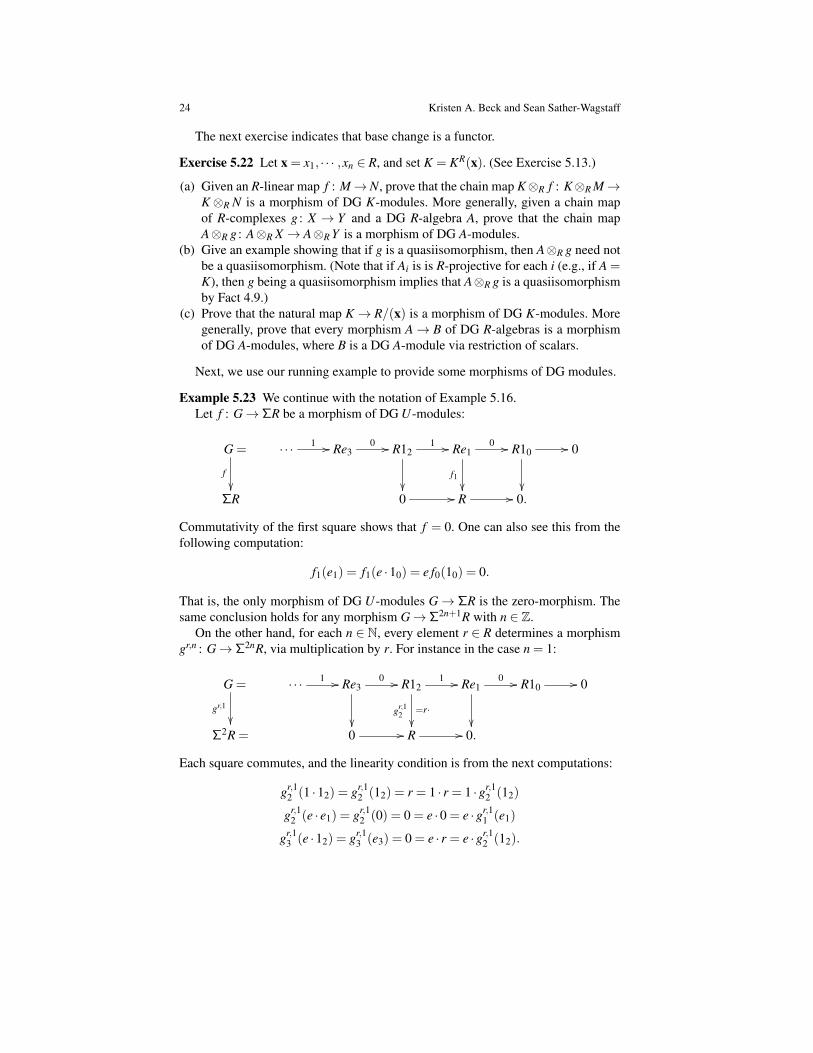
Example 5.23 We continue with the notation of Example 5.16.Let f : G→ ΣR be a morphism of DG U-modules:
G =
f��
· · · 1 // Re30 // R12
1 //
��
Re10 //
f1��
R10 //
��
0
ΣR 0 // R // 0.
Commutativity of the first square shows that f = 0. One can also see this from thefollowing computation:
f1(e1) = f1(e ·10) = e f0(10) = 0.
That is, the only morphism of DG U-modules G→ ΣR is the zero-morphism. Thesame conclusion holds for any morphism G→ Σ2n+1R with n ∈ Z.
On the other hand, for each n ∈ N, every element r ∈ R determines a morphismgr,n : G→ Σ2nR, via multiplication by r. For instance in the case n = 1:
G =
gr,1
��
· · · 1 // Re30 //
��
R121 //
gr,12 =r·��
Re10 //
��
R10 // 0
Σ2R = 0 // R // 0.
Each square commutes, and the linearity condition is from the next computations:
gr,12 (1 ·12) = gr,1
2 (12) = r = 1 · r = 1 ·gr,12 (12)
gr,12 (e · e1) = gr,1
2 (0) = 0 = e ·0 = e ·gr,11 (e1)
gr,13 (e ·12) = gr,1
3 (e3) = 0 = e · r = e ·gr,12 (12).

DG commutative algebra 25
Further, the isomorphism HomR(R,R)∼= R shows that each morphism G→Σ2nR is
of the form gr,n. Also, one checks readily that the map Ggu,0−−→ R is a quasiisomor-
phism for each unit u of R.
Truncations of DG Modules
The next operation allows us to swap a given DG module with a “shorter” one; seeExercise 5.27(b).
Definition 5.24 Let A be a DG R-algebra, and let M be a DG A-module. The supre-mum of M is
sup(M) := sup{i ∈ Z | Hi(M) 6= 0}.
Given an integer n, the nth soft left truncation of M is the complex
τ(M)(6n) := 0→Mn/ Im(∂ Mn+1)→Mn−1→Mn−2→ ···
with differential induced by ∂ M .
Example 5.25 We continue with the notation of Example 5.16. For each n > 1, seti = bn/2c and prove that
τ(G)(6n) = 0→ R12i1−→ Re2i−1
0−→ ·· · 1−→ Re30−→ R12
1−→ Re10−→ R10→ 0.
Remark 5.26 Let P be a projective resolution of an R-module M, with P+ denot-ing the augmented resolution as in Example 3.2. Then one has τ(P)(60)
∼= M. Inparticular, P is a projective resolution of τ(P)(60).
Exercise 5.27 Let A be a DG R-algebra, let M be a DG A-module, and let n ∈ Z.
(a) Prove that the truncation τ(M)(6n) is a DG A-module with the induced scalarmultiplication, and the natural chain map M→ τ(M)(6n) is a morphism of DGA-modules.
(b) Prove that the morphism from part (a) is a quasiisomorphism if and only ifn > sup(M).
DG Algebra Resolutions
The following fact provides the final construction needed to give an initial sketch ofthe proof of Theorem 1.4.
Fact 5.28 Let Q→ R be a ring epimorphism. Then there is a quasiisomorphismA '−→ R of DG Q-algebras such that each Ai is finitely generated and projective overR and Ai = 0 for i > pdQ(R). See, e.g., [4, Proposition 2.2.8].

26 Kristen A. Beck and Sean Sather-Wagstaff
Definition 5.29 In Fact 5.28, the quasiisomorphism A '−→ R is a DG algebra reso-lution of R over Q.
Remark 5.30 When y ∈Q is a Q-regular sequence, the Koszul complex KQ(y) is aDG algebra resolution of Q/(y) over Q by Lemma 4.18 and Example 5.3. Section 6contains other classical examples.
Example 5.31 Let Q be a ring, and consider an ideal I ( Q. Assume that the quo-tient R := Q/I has pdQ(R)6 1. Then every projective resolution of R over Q of theform A = (0→ A1→ Q→ 0) has the structure of a DG algebra resolution.
We conclude this section with the beginning of the proof of Theorem 1.4. Therest of the proof is contained in 7.38 and 8.17.
5.32 (First part of the Proof of Theorem 1.4) There is a flat local ring homomor-phism R→ R′ such that R′ is complete with algebraically closed residue field, asin the proof of Theorem 2.13. Since there is a 1-1 function S0(R) ↪→ S0(R′) byFact 2.7, we can replace R with R′ and assume without loss of generality that R iscomplete with algebraically closed residue field.
Since R is complete and local, Cohen’s structure theorem provides a ring epi-morphism τ : (Q,n,k)→ (R,m,k) where Q is a complete regular local ring suchthat m and n have the same minimal number of generators. Let y = y1, . . . ,yn ∈ n bea minimal generating sequence for n, and set x = x1, . . . ,xn ∈ m where xi := τ(yi).It follows that we have KR(x)∼= KQ(y)⊗Q R. Since Q is regular and y is a minimalgenerating sequence for n, the Koszul complex KQ(y) is a minimal Q-free resolutionof k by Lemma 4.18.
Fact 5.28 provides a DG algebra resolution A '−→ R of R over Q. Note thatpdQ(R)< ∞ since Q is regular. We consider the following diagram of morphisms ofDG Q-algebras:
R→ KR(x)∼= KQ(y)⊗Q R '←− KQ(y)⊗Q A '−→ k⊗Q A =: U. (5.32.1)
The first map is from Exercise 5.6. The isomorphism is from the previous paragraph.The first quasiisomorphism comes from an application of KQ(y)⊗Q− to the quasi-isomorphism R '←− A, using Fact 4.9. The second quasiisomorphism comes from anapplication of −⊗Q A to the quasiisomorphism KQ(y) '−→ k. Note that k⊗Q A is afinite dimensional DG k-algebra because of the assumptions on A.
We show in 7.38 below how this provides a diagram
S0(R) ↪→S(R) ≡−→S(KR(x)) ≡←−S(KQ(y)⊗Q A) ≡−→S(U) (5.32.2)
where ≡ identifies bijections of sets. We then show in 8.17 that S(U) is finite, andit follows that S0(R) is finite, as desired.
DG commutative algebra 27
6 Examples of Algebra Resolutions
Remark 5.30 and Example 5.31 provide constructions of DG algebra resolutions, inparticular, for rings of projective dimension at most 1. The point of this section isto extend this to rings of projective dimension 2 and rings of projective dimension 3determined by Gorenstein ideals.
Definition 6.1 Let I be an ideal of a local ring (R,m). The grade of I in R, denotedgradeR(I), is defined to be the length of the longest regular sequence of R containedin I. Equivalently, we have
gradeR(I) := min{
i | ExtiR(R/I,R) 6= 0}
and it follows that gradeR(I) 6 pdR(R/I). We say that I is perfect if gradeR(I) =pdR(R/I) < ∞. In this case, ExtiR(R/I,R) is non-vanishing precisely when i =pdR(R/I). If, in addition, this single non-vanishing cohomology module is isomor-phic to R/I, then I is said to be Gorenstein.
Notation 6.2 Let A be a matrix7 over R and J,K ⊂ N. The submatrix of A obtainedby deleting columns indexed by J and rows indexed by K is denoted AJ
K . We ab-breviate A /0
{i} as Ai, and so on. Let In(A) be the ideal of R generated by the “n× nminors” of A, that is, the determinants of the n×n matrices of the form AJ
K .
Resolutions of length two
The following result, known as the Hilbert-Burch Theorem, provides a characteriza-tion of perfect ideals of grade two. It was first proven by Hilbert in 1890 in the casethat R is a polynomial ring [27]; the more general statement was proven by Burchin 1968 [13, Theorem 5].
Theorem 6.3 ([13, 27]) Let I be an ideal of the local ring (R,m).
(a) If pdR(R/I) = 2, then
(1) there is a non-zerodivisor a ∈ R such that R/I has a projective resolution of
the form 0→ Rn A−→ Rn+1 B−→ R→ 0 where B is the 1× (n+ 1) matrix withith column given by (−1)i−1adet(Ai),
(2) one has I = aIn(A), and(3) the ideal In(A) is perfect of grade 2.
(b) Conversely, if A is an (n+1)×n matrix over R such that grade(In(A))> 2, then
R/In(A) has a projective resolution of the form 0→ Rn A−→ Rn+1 B−→ R→ 0 whereB is the 1× (n+1) matrix with ith column given by (−1)i−1 det(Ai).
7 While much of the work in this section can be done basis-free, the formulations are somewhatmore transparent when bases are specified and matrices are used to represent homomorphisms.
28 Kristen A. Beck and Sean Sather-Wagstaff
Exercise 6.4 Use Theorem 6.3 to build a grade two perfect ideal I in R = k[[x,y]].
Herzog [26] showed that Hilbert-Burch resolutions can be endowed with DGalgebra structures.
Theorem 6.5 ([26]) Given an (n+1)×n matrix A over R, let B be the 1× (n+1)matrix with ith column given by (−1)i−1adet(Ai) for some non-zerodivisor a ∈ R.Then the R-complex
0→n⊕
`=1
R f`A−→
n+1⊕`=1
Re`B−→ R1→ 0
has the structure of a DG R-algebra with the following multiplication relations:
(1) e2i = 0 = f j fk and ei f j = 0 = f jei for all i, j,k, and
(2) eie j =−e jei = an
∑k=1
(−1)i+ j+k det(Aki, j) fk for all 1 6 i < j 6 n+1. 8
Exercise 6.6 Verify the Leibniz rule for the product defined in Theorem 6.5.
Exercise 6.7 Using the ideal I from Exercise 6.4, build a (minimal) free resolutionfor R/I, then specify the relations giving this resolution a DG R-algebra structure.
Resolutions of length three
We turn our attention to resolutions of length three, first recalling needed machinery.
Definition 6.8 A square matrix A over R is alternating if it is skew-symmetric andhas all 0’s on its diagonal. Let A be an n× n alternating matrix over R. If n iseven, then there is an element Pf(A) ∈ R such that Pf(A)2 = det(A). If n is oddthen det(A) = 0, so we set Pf(A) = 0. The element Pf(A) is called the Pfaffian of A.(See, e.g., [11, Section 3.4] for more details.) We denote by Pfn−1(A) the ideal of Rgenerated by the submaximal Pfaffians of A, that is,
Pfn−1(A) :=(Pf(Ai
i) | 1 6 i 6 n)
R.
Example 6.9 Let x,y,z ∈ R. For the matrix A =[
0 x−x 0
], we have det(A) = x2, so
Pf(A) = x, and Pf1(A) = 0.
For the matrix B =
[0 x y−x 0 z−y −z 0
]we have det(B) = 0 = Pf(B) and
Pf2(B) = (Pf([
0 x−x 0
]),Pf(
[0 y−y 0
]),Pf(
[ 0 z−z 0
]))R = (x,y,z)R.
8 Note that the sign in this expression differs from the one found in [4, Example 2.1.2].
DG commutative algebra 29
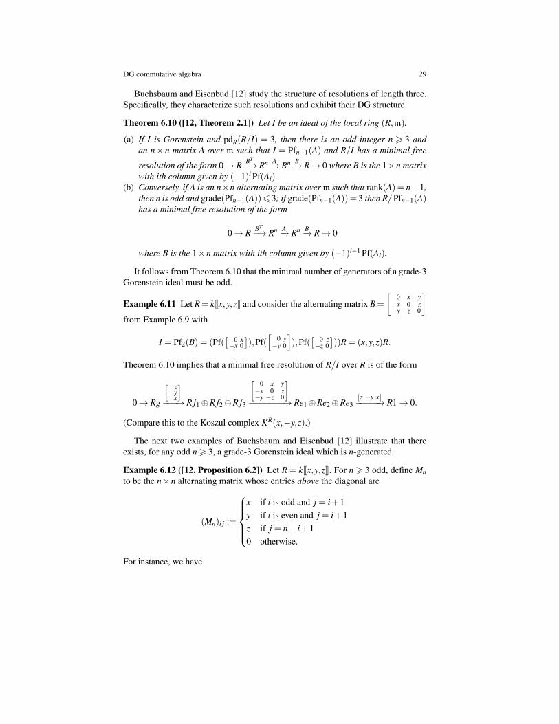
Buchsbaum and Eisenbud [12] study the structure of resolutions of length three.Specifically, they characterize such resolutions and exhibit their DG structure.
Theorem 6.10 ([12, Theorem 2.1]) Let I be an ideal of the local ring (R,m).
(a) If I is Gorenstein and pdR(R/I) = 3, then there is an odd integer n > 3 andan n× n matrix A over m such that I = Pfn−1(A) and R/I has a minimal free
resolution of the form 0→ R BT−→ Rn A−→ Rn B−→ R→ 0 where B is the 1×n matrix
with ith column given by (−1)i Pf(Ai).(b) Conversely, if A is an n×n alternating matrix over m such that rank(A) = n−1,
then n is odd and grade(Pfn−1(A))6 3; if grade(Pfn−1(A))= 3 then R/Pfn−1(A)has a minimal free resolution of the form
0→ R BT−→ Rn A−→ Rn B−→ R→ 0
where B is the 1×n matrix with ith column given by (−1)i−1 Pf(Ai).
It follows from Theorem 6.10 that the minimal number of generators of a grade-3Gorenstein ideal must be odd.
Example 6.11 Let R= k[[x,y,z]] and consider the alternating matrix B=
[0 x y−x 0 z−y −z 0
]from Example 6.9 with
I = Pf2(B) = (Pf([
0 x−x 0
]),Pf(
[0 y−y 0
]),Pf(
[ 0 z−z 0
]))R = (x,y,z)R.
Theorem 6.10 implies that a minimal free resolution of R/I over R is of the form
0→ Rg
[ z−y
x
]−−−→ R f1⊕R f2⊕R f3
[0 x y−x 0 z−y −z 0
]−−−−−−−→ Re1⊕Re2⊕Re3
[z −y x ]−−−−−→ R1→ 0.
(Compare this to the Koszul complex KR(x,−y,z).)
The next two examples of Buchsbaum and Eisenbud [12] illustrate that thereexists, for any odd n > 3, a grade-3 Gorenstein ideal which is n-generated.
Example 6.12 ([12, Proposition 6.2]) Let R = k[[x,y,z]]. For n > 3 odd, define Mnto be the n×n alternating matrix whose entries above the diagonal are
(Mn)i j :=
x if i is odd and j = i+1y if i is even and j = i+1z if j = n− i+10 otherwise.
For instance, we have
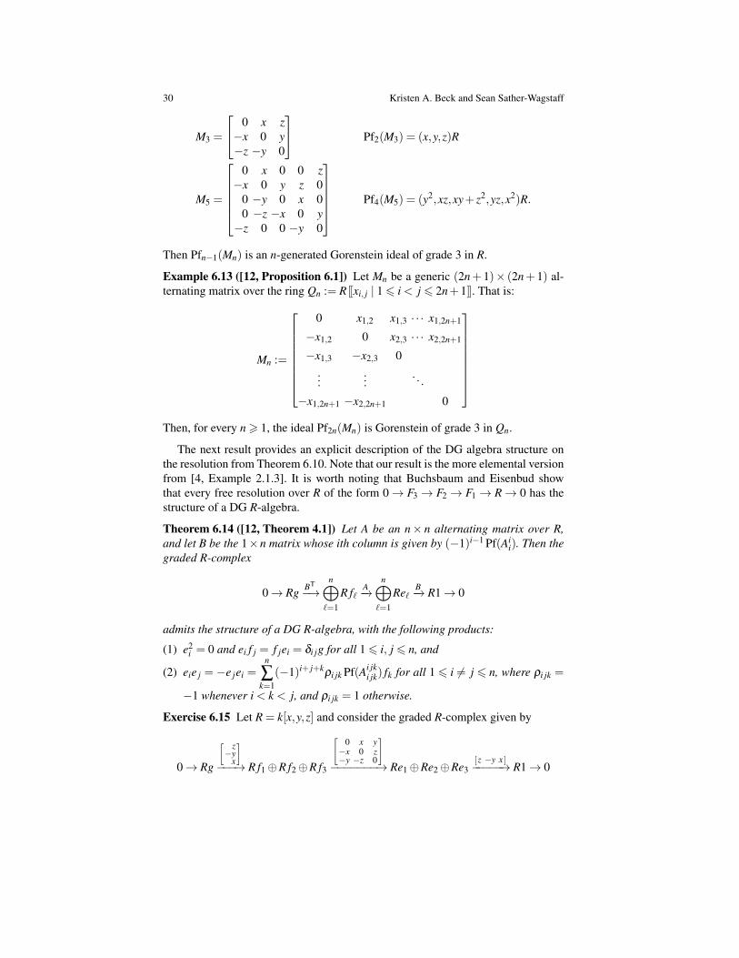
30 Kristen A. Beck and Sean Sather-Wagstaff
M3 =
0 x z−x 0 y−z −y 0
Pf2(M3) = (x,y,z)R
M5 =
0 x 0 0 z−x 0 y z 0
0 −y 0 x 00 −z −x 0 y−z 0 0 −y 0
Pf4(M5) = (y2,xz,xy+ z2,yz,x2)R.
Then Pfn−1(Mn) is an n-generated Gorenstein ideal of grade 3 in R.
Example 6.13 ([12, Proposition 6.1]) Let Mn be a generic (2n+ 1)× (2n+ 1) al-ternating matrix over the ring Qn := R [[xi, j | 1 6 i < j 6 2n+1]]. That is:
Mn :=
0 x1,2 x1,3 · · · x1,2n+1
−x1,2 0 x2,3 · · · x2,2n+1
−x1,3 −x2,3 0...
.... . .
−x1,2n+1 −x2,2n+1 0
Then, for every n > 1, the ideal Pf2n(Mn) is Gorenstein of grade 3 in Qn.
The next result provides an explicit description of the DG algebra structure onthe resolution from Theorem 6.10. Note that our result is the more elemental versionfrom [4, Example 2.1.3]. It is worth noting that Buchsbaum and Eisenbud showthat every free resolution over R of the form 0→ F3 → F2 → F1 → R→ 0 has thestructure of a DG R-algebra.
Theorem 6.14 ([12, Theorem 4.1]) Let A be an n× n alternating matrix over R,and let B be the 1×n matrix whose ith column is given by (−1)i−1 Pf(Ai
i). Then thegraded R-complex
0→ Rg BT
−→n⊕
`=1
R f`A−→
n⊕`=1
Re`B−→ R1→ 0
admits the structure of a DG R-algebra, with the following products:
(1) e2i = 0 and ei f j = f jei = δi jg for all 1 6 i, j 6 n, and
(2) eie j = −e jei =n
∑k=1
(−1)i+ j+kρi jk Pf(Ai jk
i jk) fk for all 1 6 i 6= j 6 n, where ρi jk =
−1 whenever i < k < j, and ρi jk = 1 otherwise.
Exercise 6.15 Let R = k[x,y,z] and consider the graded R-complex given by
0→ Rg
[ z−y
x
]−−−→ R f1⊕R f2⊕R f3
[0 x y−x 0 z−y −z 0
]−−−−−−−→ Re1⊕Re2⊕Re3
[z −y x ]−−−−−→ R1→ 0

DG commutative algebra 31
Using Theorem 6.14, write the product relations that give this complex the structureof a DG R-algebra.
Longer resolutions
In general, resolutions of length greater than 3 are not guaranteed to possess a DGalgebra structure, as the next example of Avramov shows.
Example 6.16 ([4, Theorem 2.3.1]) Consider the local ring R = k[[w,x,y,z]]. Thenthe minimal free resolutions over R of the quotients R/(w2,wx,xy,yz,z2)R andR/(w2,wx,xy,yz,z2,wy6,x7,x6z,y7)R do not admit DG R-algebra structures.
On the other hand, resolutions of ideals I with pdR(R/I)> 4 that are sufficientlynice do admit DG algebra structures. For instance, Kustin and Miller prove the fol-lowing in [28, Theorem] and [29, 4.3 Theorem].
Example 6.17 ([28, 29]) Let I be a Gorenstein ideal of a local ring R. If pdR(R/I) =4, then the minimal R-free resolution of R/I has the structure of a DG R-algebra.
7 DG Algebras and DG Modules II
In this section, we describe the notions needed to define semidualizing DG modulesand to explain some of their base-change properties. This includes a discussion oftwo types of Ext for DG modules. The section concludes with another piece of theproof of Theorem 1.4; see 8.17.
Convention 7.1 Throughout this section, A is a DG R-algebra, and L, M, and N areDG A-modules.
Hom for DG Modules
The semidualizing property for R-modules is defined in part by a Hom condition, sowe begin our treatment of the DG-version with Hom.
Definition 7.2 Given an integer i, a DG A-module homomorphism of degree n is anelement f ∈ HomR(M,N)n such that fi+ j(am) = (−1)nia f j(m) for all a ∈ Ai andm ∈ M j. The graded submodule of HomR(M,N) consisting of all DG A-modulehomomorphisms M→ N is denoted HomA(M,N).
Part (b) of the next exercise gives another hint of the semidualizing property forDG modules.
32 Kristen A. Beck and Sean Sather-Wagstaff
Exercise 7.3
(a) Prove that HomA(M,N) is a DG A-module via the action
(a f ) j(m) := a( f j(m)) = (−1)|a|| f | f j+|a|(am)
and using the differential from HomR(M,N).(b) Prove that for each a ∈ A the multiplication map µM,a : M→M given by m 7→
am is a homomorphism of degree |a|.(c) Prove that f ∈HomA(M,N)0 is a morphism if and only if it is a cycle, that is, if
and only if ∂HomA(M,N)0 ( f ) = 0.
Example 7.4 We continue with the notation of Example 5.16. From computationslike those in Example 5.23, it follows that HomU (G,R) has the form
HomU (G,R) = 0→ R→ 0→ R→ 0→ ···
where the copies of R are in even non-positive degrees. Multiplication by e is 0 onHomU (G,R), by degree considerations, and multiplication by 1 is the identity.
Next, we give an indication of the functoriality of HomA(N,−) and HomA(−,N).
Definition 7.5 Given a morphism f : L → M of DG A-modules, we define themap HomA(N, f ) : HomA(N,L)→ HomA(N,M) as follows: each sequence {gp} ∈HomA(N,L)n is mapped to { fp+ngp} ∈ HomA(N,M)n. Similarly, define the mapHomA( f ,N) : HomA(M,N)→ HomA(L,N) by the formula {gp} 7→ {gp fp}.
Remark 7.6 We do not use a sign-change in this definition because | f |= 0.
Exercise 7.7 Given a morphism f : L→M of DG A-modules, prove that the mapsHomA(N, f ) and HomA( f ,N) are well-defined morphisms of DG A-modules.
Tensor Product for DG Modules
As with modules and complexes, we use the tensor product to base change DGmodules along a morphism of DG algebras.
Definition 7.8 The tensor product M⊗A N is the quotient (M⊗R N)/U where U isgenerated over R by the elements of the form (am)⊗ n− (−1)|a||m|m⊗ (an). Givenan element m⊗ n ∈M⊗R N, we denote the image in M⊗A N as m⊗ n.
Exercise 7.9 Prove that the tensor product M⊗A N is a DG A-module via the scalarmultiplication
a(m⊗ n) := (am)⊗ n = (−1)|a||m|m⊗ (an).
The next exercises describe base change and some canonical isomorphisms forDG modules.

DG commutative algebra 33
Exercise 7.10 Let A→ B be a morphism of DG R-algebras. Prove that B⊗A M hasthe structure of a DG B-module by the action b(b′⊗m) := (bb′)⊗m. Prove that thisstructure is compatible with the DG A-module structure on B⊗A M via restrictionof scalars.
Exercise 7.11 Verify the following isomorphisms of DG A-modules:
HomA(A,L)∼= L Hom cancellationA⊗A L∼= L tensor cancellation
L⊗A M ∼= M⊗A L tensor commutativity
In particular, there are DG A-module isomorphisms HomA(A,A)∼= A∼= A⊗A A.
Fact 7.12 There is a natural “Hom tensor adjointness” DG A-module isomorphismHomA(L⊗A M,N)∼= HomA(M,HomA(L,N)).
Next, we give an indication of the functoriality of N⊗A− and −⊗A N.
Definition 7.13 Given a morphism f : L → M of DG A-modules, we define themap N⊗A f : N⊗A L→ N⊗A M by the formula z⊗ y 7→ z⊗ f (y). Define the mapf ⊗A N : L⊗A N→M⊗A N by the formula x⊗ z 7→ f (x)⊗ z.
Remark 7.14 We do not use a sign-change in this definition because | f |= 0.
Exercise 7.15 Given a morphism f : L→M of DG A-modules, prove that the mapsN⊗A f and f ⊗R N are well-defined morphisms of DG A-modules.
Semifree Resolutions
Given the fact that the semidualizing property includes an Ext-condition, it shouldcome as no surprise that we need a version of free resolutions in the DG setting.
Definition 7.16 A subset E of L is called a semibasis if it is a basis of the underlyingA\-module L\. If L is bounded below, then L is called semi-free if it has a semibasis.9
A semi-free resolution of a DG A-module M is a quasiisomorphism F '−→M of DGA-modules such that F is semi-free.
The next exercises and example give some semi-free examples to keep in mind.
Exercise 7.17 Prove that a semi-free DG R-module is simply a bounded belowcomplex of free R-modules. Prove that each free resolution F of an R-module Mgives rise to a semi-free resolution F '−→M; see Exercise 3.10.
9 As is noted in [6], when L is not bounded below, the definition of “semi-free” is more technical.However, our results do not require this level of generality, so we focus only on this case.

34 Kristen A. Beck and Sean Sather-Wagstaff
Exercise 7.18 Prove that M is exact (as an R-complex) if and only if 0 '−→ M is asemi-free resolution. Prove that the DG A-module ΣnA is semi-free for each n ∈ Z,as is
⊕n>n0
ΣnAβn for all n0 ∈ Z and βn ∈ N.
Exercise 7.19 Let x = x1, · · · ,xn ∈ R, and set K = KR(x).
(a) Given a bounded below complex F of free R-modules, prove that the complexK⊗R F is a semi-free DG K-module.
(b) If F '−→M is a free resolution of an R-module M, prove that K⊗R F '−→K⊗R M isa semi-free resolution of the DG K-module K⊗R M. More generally, if F '−→Mis a semi-free resolution of a DG R-module M, prove that K⊗R F '−→ K⊗R M isa semi-free resolution of the DG K-module K⊗R M. See Fact 4.9.
Example 7.20 In the notation of Example 5.16, the natural map g1,0 : G→ R is asemi-free resolution of R over U ; see Example 5.23. The following display indicateswhy G is semi-free over U , that is, why G\ is free over U \:
U = 0→ Re 0−→ R1→ 0
U \ = Re⊕
R1
G = · · · 1−→ Re30−→ R12
1−→ Re10−→ R10→ 0
G\ = · · ·(Re3⊕
R12)⊕
(Re1⊕
R10).
The next item compares to Remark 5.26.
Remark 7.21 If L is semi-free, then the natural map L→ τ(L)(6n) is a semi-freeresolution for each n > sup(L).
The next facts contain important existence results for semi-free resolutions. No-tice that the second paragraph applies when A is a Koszul complex over R or is finitedimensional over a field, by Exercise 5.10.
Fact 7.22 The DG A-module M has a semi-free resolution if and only if Hi(M) = 0for i� 0, by [6, Theorem 2.7.4.2].
Assume that A is noetherian, and let j be an integer. Assume that each moduleHi(M) is finitely generated over H0(A) and that Hi(M) = 0 for i < j. Then M has asemi-free resolution F '−→M such that F\ ∼=
⊕∞i= j Σ
i(A\)βi for some integers βi, andso Fi = 0 for all i < j; see [1, Proposition 1]. In particular, homologically finite DGA-modules admit “degree-wise finite, bounded below” semi-free resolutions.
Fact 7.23 Assume that L and M are semi-free. If there is a quasiisomorphism L '−→M, then there is also a quasiisomorphism M '−→ L by [4, Proposition 1.3.1].
The previous fact explains why the next relations are symmetric. The fact thatthey are reflexive and transitive are straightforward to verify.
DG commutative algebra 35
Definition 7.24 Two semi-free DG A-modules L and M are quasiisomorphic ifthere is a quasiisomorphism L '−→ M; this equivalence relation is denoted by thesymbol'. Two semi-free DG A-modules L and M are shift-quasiisomorphic if thereis an integer m such that L' ΣmM; this equivalence relation is denoted by ∼.
Semidualizing DG Modules
For Theorem 1.4, we use a version of Christensen and Sather-Wagstaff’s notion ofsemidualizing DG modules from [16], defined next.
Definition 7.25 The homothety morphism χAM : A→ HomA(M,M) is given by the
formula (χAM)|a|(a) := µM,a, i.e., (χA
M)|a|(a)|m|(m) = am.Assume that A is noetherian. Then M is a semidualizing DG A-module if M is
homologically finite and semi-free such that χAM : A→ HomA(M,M) is a quasiiso-
morphism. Let S(A) denote the set of shift-quasiisomorphism classes of semidu-alizing DG A-modules, that is, the set of equivalence classes of semidualizing DGA-modules under the relation ∼ from Definition 7.24.
Exercise 7.26 Prove that the homothety morphism χAM : A → HomA(M,M) is a
well-defined morphism of DG A-modules.
The following fact explains part of diagram (5.32.2).
Fact 7.27 Let M be an R-module with projective resolution P. Then Fact 3.18 showsthat M is a semidualizing R-module if and only if P is a semidualizing DG R-module. It follows that we have an injection S0(R) ↪→S(R).
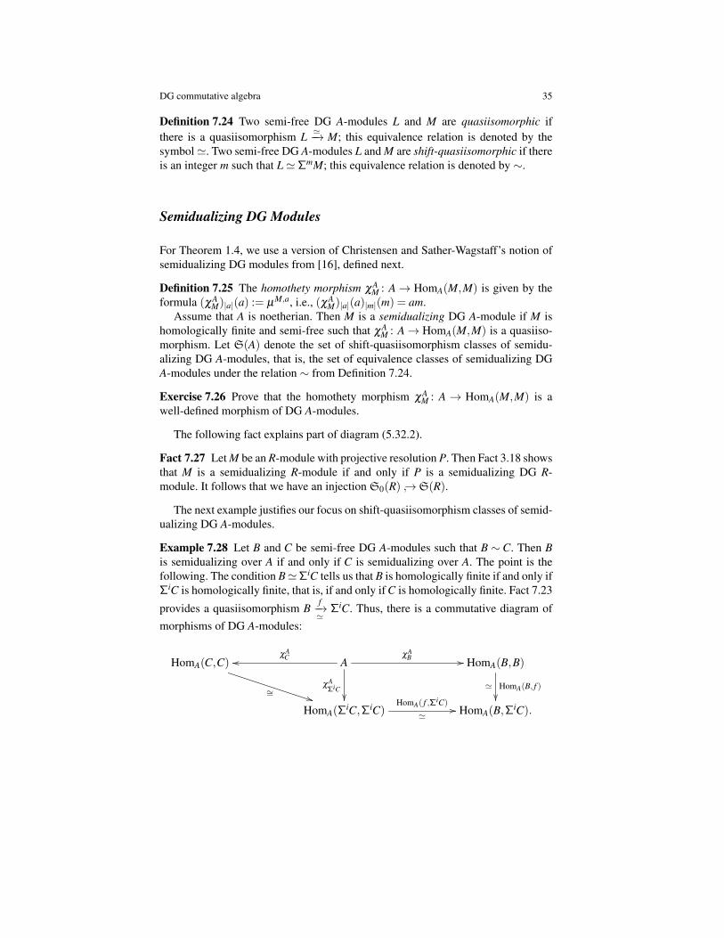
The next example justifies our focus on shift-quasiisomorphism classes of semid-ualizing DG A-modules.
Example 7.28 Let B and C be semi-free DG A-modules such that B ∼ C. Then Bis semidualizing over A if and only if C is semidualizing over A. The point is thefollowing. The condition B'ΣiC tells us that B is homologically finite if and only ifΣiC is homologically finite, that is, if and only if C is homologically finite. Fact 7.23
provides a quasiisomorphism Bf−→'
ΣiC. Thus, there is a commutative diagram ofmorphisms of DG A-modules:
HomA(C,C)
∼= **
AχA
Coo χAB //
χAΣiC��
HomA(B,B)
HomA(B, f )'��
HomA(ΣiC,ΣiC)
HomA( f ,ΣiC)
'// HomA(B,ΣiC).

36 Kristen A. Beck and Sean Sather-Wagstaff
The unspecified isomorphism follows from a bookkeeping exercise.10 The mor-phisms HomA( f ,C) and HomA(B, f ) are quasiisomorphisms by [4, Propositions1.3.2 and 1.3.3] because B and ΣiC are semi-free and f is a quasiisomorphism.It follows that χA
B is a quasiisomorphism if and only if χAΣiC is a quasiisomorphism
if and only if χAC is a quasiisomorphism.
The following facts explain other parts of (5.32.2).
Fact 7.29 Assume that (R,m) is local. Fix a list of elements x ∈ m and set K =KR(x). Base change K⊗R− induces an injective map S(R) ↪→S(K) by [16, A.3.Lemma]; if R is complete, then this map is bijective by [33, Corollary 3.10].
Fact 7.30 Let ϕ : A '−→B be a quasiisomorphism of noetherian DG R-algebras. Basechange B⊗A− induces a bijection from S(A) to S(B) by [32, Lemma 2.22(c)].
Ext for DG Modules
One subtlety in the proof of Fact 7.29 is found in the behavior of Ext for DG mod-ules, which we describe next.
Definition 7.31 Given a semi-free resolution F '−→ M, for each integer i we setExtiA(M,N) := H−i(HomA(F,N)).11
The next two items are included in our continued spirit of providing perspective.
Exercise 7.32 Given R-modules M and N, prove that the module ExtiR(M,N) de-fined in 7.31 is the usual ExtiR(M,N); see Exercise 7.17.
Example 7.33 In the notation of Example 5.16, Examples 7.4 and 7.20 imply
ExtiU (R,R) = H−i(HomU (G,R)) =
{R if i > 0 is even0 otherwise.
Contrast this with the equality ExtiU\(R,R) = R for all i > 0. This shows that U isfundamentally different from U \ ∼= R[X ]/(X2), even though U is obtained using atrivial differential on R[X ]/(X2) with the natural grading.
The next result compares with the fact that ExtiR(M,N) is independent of thechoice of free resolution when M and N are modules.
Fact 7.34 For each index i, the module ExtiA(M,N) is independent of the choice ofsemi-free resolution of M by [4, Proposition 1.3.3].
10 The interested reader may wish to show how this isomorphism is defined and to check thecommutativity of the diagram. If this applies to you, make sure to mind the signs.11 One can also define TorR
i (M,N) := Hi(F⊗A N), but we do not need this here.

DG commutative algebra 37
Remark 7.35 An important fact about Ext1R(M,N) for R-modules M and N is thefollowing: the elements of Ext1R(M,N) are in bijection with the equivalence classesof short exact sequences (i.e., “extensions”) of the form 0→ N→ X →M→ 0. ForDG modules over a DG R-algebra A, things are a bit more subtle.
Given DG A-modules M and N, one defines the notion of a short exact sequenceof the form 0→ N → X →M→ 0 in the naive way: the arrows are morphisms ofDG A-modules such that for each i ∈ Z the sequence 0→ Ni → Xi → Mi → 0 isexact. One defines an equivalence relation on the set of short exact sequences of this
form (i.e., “extensions”) in the natural way: two extensions 0→ Nf−→ X
g−→M→ 0
and 0→ Nf ′−→ X ′
g′−→M→ 0 are equivalent if there is a commutative diagram
0 // Nf //
=
��
Xg //
h��
M //
=
��
0
0 // Nf ′ // X ′
g′ // M // 0
of morphisms of DG A-modules. Let YExt1A(M,N) denote the set of equivalenceclasses of such extensions. (The “Y” is for “Yoneda”.) As with R-modules, one candefine an abelian group structure on YExt1A(M,N). However, in general one hasYExt1A(M,N)� Ext1A(M,N), even when A = R, as the next example shows.
Example 7.36 Let R = k[[X ]], and consider the following exact sequence of DGR-modules, i.e., exact sequence of R-complexes:
0 // R // R // k // 0
0
��
0
��
0
��0 // R X //
1 ��
R //
1 ��
k //
1 ��
0
0 // R X //
��
R //
��
k //
��
0
0 0 0.
This sequence does not split over R (it is not even degree-wise split) so it givesa non-trivial class in YExt1R(k,R), and we conclude that YExt1R(k,R) 6= 0. On theother hand, k is homologically trivial, so we have Ext1R(k,R) = 0 since 0 '−→ k is asemi-free resolution.
For our proof of Theorem 1.4, the following connection between Ext and YExtis quite important; see [32, Corollary 3.8 and Proposition 3.12].
Fact 7.37 If L is semi-free, then we have YExt1A(L,M)∼=Ext1A(L,M); if furthermoreExt1R(L,L) = 0, then for each n > sup(L), one has

38 Kristen A. Beck and Sean Sather-Wagstaff
YExt1A(L,L) = 0 = YExt1A(τ(L)(6n),τ(L)(6n)).
We conclude this section with the second part of the proof of Theorem 1.4. Therest of the proof is contained in 8.17.
7.38 (Second part of the proof of Theorem 1.4) We continue with the notation es-tablished in 5.32. The properties of diagram (5.32.2) follow from diagram (5.32.1)because of Facts 7.29 and 7.30. Thus, it remains to show that S(k⊗Q A) is finite.This is shown in 8.17.
8 A Version of Happel’s Result for DG Modules
This section contains the final steps of the proof of Theorem 1.4; see 8.17. Theidea, from [2, 22, 25, 42] is a bold one: use algebraic geometry to study all possiblemodule structures on a fixed set. A simple case of this is in Example 5.17. We beginwith some notation for use throughout this section.
Notation 8.1 Let F be an algebraically closed field, and let
U := (0→Uq∂U
q−→Uq−1∂U
q−1−−→ ·· ·∂U
1−→U0→ 0)
be a finite-dimensional DG F-algebra. Let dimF(Ui) = ni for i = 0, . . . ,q. Let
W :=s⊕
i=0
Wi
be a graded F-vector space with ri := dimF(Wi) for i = 0, . . . ,s.A DG U-module structure on W consists of two pieces of data. First, we need
a differential ∂ . Second, once the differential ∂ has been chosen, we need a scalarmultiplication µ . Let ModU (W ) denote the set of all ordered pairs (∂ ,µ) making Winto a DG U-module. Let EndF(W )0 denote the set of F-linear endomorphisms ofW that are homogeneous of degree 0. Let GL(W )0 denote the set of F-linear auto-morphisms of W that are homogeneous of degree 0, that is, the invertible elementsof EndF(W )0.
We next describe a geometric structure on ModU (W ), as in Example 5.17.
Discussion 8.2 We work in the setting of Notation 8.1.A differential ∂ on W is an element of the graded vector space HomF(W,W )−1 =⊕s
i=0 HomF(Wi,Wi−1) such that ∂∂ = 0. The vector space HomF(Wi,Wi−1) has di-mension riri−1, so the map ∂ corresponds to an element of the affine space Ad
Fwhere d := ∑i riri−1. The vanishing condition ∂∂ = 0 is equivalent to the entries ofthe matrices representing ∂ satisfying certain fixed homogeneous quadratic polyno-mial equations over F . Hence, the set of all differentials on W is a Zariski-closedsubset of Ad
F .
DG commutative algebra 39
Once the differential ∂ has been chosen, a scalar multiplication µ is in particulara cycle in HomF(U⊗F W,W )0 =
⊕i, j HomF(Ui⊗F Wj,Wi+ j). For all i, j, the vector
space HomF(Ui⊗F Wj,Wi+ j) has dimension nir jri+ j, so the map µ corresponds toan element of the affine space Ad′
F where d′ := ∑i, j nir jri+ j. The condition that µ bean associative, unital cycle is equivalent to the entries of the matrices representing∂ and µ satisfying certain fixed polynomials over F . Thus, the set ModU (W ) is aZariski-closed subset of Ad
F ×Ad′F∼= Ad+d′
F .
Example 8.3 We continue with the notation of Example 5.17. In this example, wehave ModU (W ) = {1} (representing the non-trivial scalar multiplication by 1) andModU (W ′)= {(x1,x0)∈F2 | x1x0 = 0}. Re-writing Fn asAn
F , we see that ModU (W )is a single point in A1
F and ModU (W ′) is the union of the two coordinate axesV (x1x0) =V (x0)∪V (x1).
Exercise 8.4 Continue with the notation of Example 5.17. Write out the coordinatesand equations describing ModU (W ′′) and ModU (W ′′′) where
W ′′ = 0⊕
Fw2⊕
Fw1⊕
Fw0⊕
0
W ′′′ = 0⊕
Fz2⊕
(Fz1,1⊕
Fz1,2)⊕
Fz0⊕
0.
For scalar multiplication, note that since multiplication by 1 is already determinedby the F-vector space structure, we only need to worry about multiplication by ewhich maps W ′′i →W ′′i+1 and W ′′′i →W ′′′i+1 for i = 0,1,2.
We next describe a geometric structure on the set GL(W )0.
Discussion 8.5 We work in the setting of Notation 8.1.A map α ∈ GL(W )0 is an element of the graded vector space HomF(W,W )0 =⊕s
i=0 HomF(Wi,Wi) with a multiplicative inverse. The vector space HomF(Wi,Wi)has dimension r2
i , so the map α corresponds to an element of the affine spaceAe
F where e := ∑i r2i . The invertibility of α is equivalent to the invertibility of
each “block” αi ∈ HomF(Wi,Wi), which is an open condition defined by the non-vanishing of the determinant polynomial. Thus, the set GL(W )0 is a Zariski-opensubset of Ae
F , so it is smooth over F .Alternately, one can view GL(W )0 as the product GL(W0)×·· ·×GL(Ws). Since
each GL(Wi) is an algebraic group smooth over F , it follows that GL(W )0 is also analgebraic group that is smooth over F .
Example 8.6 We continue with the notation of Example 5.17. It is straightforwardto show that
EndF(W )0 = HomF(Fν0,Fν0)∼= F = A1F
GLF(W )0 = AutF(Fν0)∼= F× =Ux ⊂ A1F
EndF(W ′)0 = HomF(Fη1,Fη1)⊕
HomF(Fη0,Fη0)∼= F×F = A2F
GLF(W ′)0 = AutF(Fη1)⊕
AutF(Fη0)∼= F××F× =Ux1x0 ⊂ A2F .

40 Kristen A. Beck and Sean Sather-Wagstaff
Here Ux is the subset A1F rV (x), and Ux1x0 = A2
F rV (x1x0).
Exercise 8.7 With the notation of Example 5.17. Give coordinates and equationsdescribing GLU (W ′′)0 and GLU (W ′′′)0 where W ′′ and W ′′′ are from Exercise 8.4.
Next, we describe an action of GL(W )0 on ModU (W ).
Discussion 8.8 We work in the setting of Notation 8.1.Let α ∈ GL(W )0. For every (∂ ,µ) ∈ModU (W ), we define α · (∂ ,µ) := (∂ , µ),
where ∂i := αi−1 ◦∂i ◦α−1i and µi+ j := αi+ j ◦µi+ j ◦ (U ⊗F α
−1j ). For the multipli-
cation, this defines a new multiplication
ui ·α w j := αi+ j(ui ·α−1j (w j))
where · is multiplication given by µ , as in Discussion 8.2: ui ·w j := µi+ j(ui⊗w j).Note that this leaves multiplication by 1A unaffected:
1A ·α w j = α j(1A ·α−1j (w j)) = α j(α
−1j (w j)) = w j.
It is routine to show that the ordered pair (∂ , µ) describes a DG U-module structurefor W , that is, we have α · (∂ ,µ) := (∂ , µ) ∈ ModU (W ). From the definition ofα · (∂ ,µ), it follows readily that this describes a GL(W )0-action on ModU (W ).
Example 8.9 Continue with the notation of Example 5.17.In this case, the only DG U-module structure on W is the trivial one (∂ ,µ) =
(0,0), so we have α · (∂ ,µ) = (∂ ,µ) for all α ∈ GL(W )0.The action of GL(W ′)0 on ModU (W ′) is a bit more interesting. Let x0,x1 ∈ F
such that x0x1 = 0, as in Example 5.17. Identify GLF(W ′)0 with F××F×, as inExample 8.3, and let α ∈GLF(W ′)0 be given by the ordered pair (y1,y0)∈F××F×.The differential ∂ is defined so that the following diagram commutes.
∂ : 0 // Fη1x1 //
y1
��
Fη0 //
y0
��
0
∂ : 0 // Fη1x1 // Fη0 // 0
so we have ∂1(η1) = y0x1y−11 η0, i.e., x1 = y0x1y−1
1 .Since multiplication by 1 is already determined, and we have e ·α η1 = 0 because
of degree considerations, we only need to understand e ·α η0. From Discussion 8.8,this is given by
e ·α η0 = α1(e ·α−10 (η0)) = α1(e · y−1
0 η0) = y−10 α1(e ·η0)
= y−10 α1(x0η1) = y−1
0 y1x0η1.

DG commutative algebra 41
Exercise 8.10 Continue with the notation of Example 5.17. Using the solutions toExercises 8.4 and 8.7 describe the actions of GL(W ′′)0 and GL(W ′′′)0 on ModU (W ′′)and ModU (W ′′′), respectively, as in the previous example.
Next, we describe some properties of the action from Discussion 8.8 that indicatea deeper connection between the algebra and geometry.
Discussion 8.11 We work in the setting of Notation 8.1.Let α ∈ GL(W )0. For every (∂ ,µ) ∈ModU (W ), let α · (∂ ,µ) := (∂ , µ) be as in
Discussion 8.8. It is straightforward to show that a map α gives a DG U-moduleisomorphism (W,∂ ,µ)
∼=−→ (W, ∂ , µ). Conversely, given another element (∂ ′,µ ′) ∈ModU (W ), if there is a DG U-module isomorphism β : (W,∂ ,µ)
∼=−→ (W,∂ ′,µ ′),then β ∈ GL(W )0 and (∂ ′,µ ′) = β · (∂ ,µ). In other words, the orbits in ModU (W )under the action of GL(W )0 are the isomorphism classes of DG U-module structureson W . Given an element M = (∂ ,µ) ∈ModU (W ), the orbit GL(W )0 ·M is locallyclosed in ModU (W ); see [18, Chapter II, §5.3].
Note that the maps defining the action of GL(W )0 on ModU (W ) are regular, thatis, determined by polynomial functions. This is because the inversion map α 7→α−1 on GL(W )0 is regular, as is the multiplication of matrices corresponding to thecompositions defining ∂ and µ .
Next, we consider even more geometry by identifying tangent spaces to two ofour objects of study.
Notation 8.12 We work in the setting of Notation 8.1. Let F [ε] := Fε⊕
F be thealgebra of dual numbers, where ε2 = 0 and |ε| = 0. For our convenience, we writeelements of F [ε] as column vectors: aε + b = [a
b ]. We identify U [ε] := F [ε]⊗F Uwith Uε
⊕U ∼= U
⊕U , and W [ε] := F [ε]⊗F W with Wε
⊕W ∼= W
⊕W . Using
this protocol, we have ∂U [ε]i =
[∂U
i 00 ∂U
i
].
Let ModU [ε](W [ε]) denote the set of all ordered pairs (∂ ,µ) making W [ε] into aDG U [ε]-module. Let EndF [ε](W [ε])0 denote the set of F [ε]-linear endomorphismsof W [ε] that are homogeneous of degree 0. Let GL(W [ε])0 denote the set of F [ε]-linear automorphisms of W [ε] that are homogeneous of degree 0, that is, the invert-ible elements of EndF [ε](W [ε])0.
Given an element M = (∂ ,µ) ∈ ModU (W ), the tangent space TModU (W )M is the
set of all ordered pairs (∂ ,µ) ∈ModU [ε](W [ε]) that give rise to M modulo ε . Thetangent space TGL(W )0
idWis the set of all elements of GL(W [ε])0 that give rise to idW
modulo ε .
Remark 8.13 Alternate descriptions of the tangent spaces from Notation 8.12 arecontained in [32, Lemmas 4.8 and 4.10]. Because of smoothness conditions, themap GL(W )0
·M−→ModU (W ) induces a linear transformation TGL(W )0idW
→ TModU (W )M
whose image is TGL(W )0·MM ; see [32, 4.11. Proof of Theorem B].

42 Kristen A. Beck and Sean Sather-Wagstaff
The next two results show some profound connections between the algebra andthe geometry of the objects under consideration. The ideas behind these results aredue to Voigt [42] and Gabriel [22, 1.2 Corollary].
Theorem 8.14 ([32, 4.11. Proof of Theorem B]) We work in the setting of Nota-tion 8.1. Given an element M = (∂ ,µ) ∈ ModU (W ), there is an isomorphism ofabelian groups
TModU (W )M /TGL(W )0·M
M∼= YExt1U (M,M).
Proof (Sketch of proof). Using Notation 8.12, let N = (∂ ,µ) be an element of
TModU (W )M . Since N is a DG U [ε]-module, restriction of scalars along the natural
inclusion U →U [ε] makes N a DG U-module.Define ρ : M→N and π : N→M by the formulas ρ(w) := [w
0 ] and π([
w′w
]):=w.
With [32, Lemmas 4.8 and 4.10], one shows that ρ and π are chain maps and that ρ
and π are U-linear. In other words, we have an exact sequence
0→Mρ→ N π→M→ 0
of DG U-module morphisms. So, we obtain a map τ : TModU (W )M → YExt1U (M,M)
where τ(N) is the equivalence class of the displayed sequence in YExt1U (M,M). Oneshows that τ is a surjective abelian group homomorphism with Ker(τ) = TGL(W )0·M
M ,and the result follows from the First Isomorphism Theorem.
To show that τ is surjective, fix an arbitrary element ζ ∈ YExt1U (M,M), repre-
sented by the sequence 0→Mf−→ Z
g−→M→ 0. In particular, this is an exact sequenceof F-complexes, so it is degree-wise split. This implies that we have a commutativediagram of graded vector spaces:
0 // Mf //
=
��
Z
ϑ
��
g // M //
=
��
0
0 // Mρ // W [ε]
π // M // 0
where ρ(w) = [w0 ], π
([w′w
])= w, and ϑ is an isomorphism of graded F-vector
spaces. The map ϑ allows us to endow W [ε] with a DG U [ε]-module structure (∂ ,µ)
that gives rise to M modulo ε . So we have N := (∂ ,µ) ∈ TModU (W )M . Furthermore,
we have τ(N) = ζ , so τ is surjective.See [32, 4.11. Proof of Theorem B] for more details. ut
Corollary 8.15 ([32, Corollary 4.12]) We work in the setting of Notation 8.1. LetC be a semidualizing DG U-module, and let s > sup(C). Set M = τ(C)(6s) andW = M\. Then the orbit GL(W )0 ·M is open in ModU (W ).
Proof. Fact 7.37 implies that YExt1U (M,M) = 0, so TModU (W )M = TGL(W )0·M
M by The-orem 8.14. As the orbit GL(W )0 ·M is smooth and locally closed, this implies thatGL(W )0 ·M is open in ModU (W ). See [32, Corollary 4.12] for more details. ut

DG commutative algebra 43
We are now in a position to state and prove our version of Happel’s result [25,proof of first proposition in section 3] that was used in the proof of Theorem 2.13.
Lemma 8.16 ([32, Lemma 5.1]) We work in the setting of Notation 8.1. The setSW (U) of quasiisomorphism classes of semi-free semidualizing DG U-modules Csuch that s > sup(C), Ci = 0 for all i < 0, and (τ(C)(6s))
\ ∼=W is finite.
Proof. Fix a representative C for each quasiisomorphism class in SW (U), and write[C] ∈SW (U) and MC = τ(C)(6s).
Let [C], [C′] ∈SW (U). If GL(W )0 ·MC = GL(W )0 ·MC′ , then [C] = [C′]: indeed,Discussion 8.8 explains the second step in the next display
C 'MC ∼= MC′ 'C′
and the remaining steps follow from the assumptions s > sup(C) and s > sup(C′),by Exercise 5.27.
Now, each orbit GL(W )0 ·MC is open in ModU (W ) by Corollary 8.15. SinceModU (W ) is a subset of an affine space over F , it is quasi-compact, so it can onlyhave finitely many open orbits. By the previous paragraph, this implies that thereare only finitely many distinct elements [C] ∈SW (U). ut
We conclude this section with the third and final part of the proof of Theorem 1.4.
8.17 (Final part of the proof of Theorem 1.4) We need to prove that S(U) is fi-nite where U = k⊗Q A. Set s = dim(R)− depth(R) + n. One uses various ac-counting principles to prove that every semidualizing DG U-module is equivalentto a semidualizing DG U-module C′ such that Hi(C′) = 0 for all i < 0 and for alli > s. Let L '−→ C′ be a minimal semi-free resolution of C′ over U . The conditionssup(L) = sup(C′)6 s imply that L (and hence C′) is quasiisomorphic to the trunca-tion L := τ(L)6s. We set W := L\ and work in the setting of Notation 8.1.
One then uses further accounting principles to prove that there is an integer λ > 0,depending only on R and U , such that ∑
si=0 ri 6 λ . Compare this with Lemma 2.9.
(Recall that ri and other quantities are fixed in Notation 8.1.) Then, because thereare only finitely many (r0, . . . ,rs) ∈ Ns+1 with ∑
si=0 ri 6 λ , there are only finitely
many W that occur from this construction, say W (1), . . . ,W (b). Lemma 8.16 impliesthat S(U) =SW (1)(U)∪·· ·∪SW (b)(U)∪{[U ]} is finite. ut
9 Applications of Semidualizing Modules
This section contains three applications of semidualizing modules, to indicate whyTheorem 1.4 might be interesting.
Assumption 9.1 Throughout this section, (R,m,k) is local.
44 Kristen A. Beck and Sean Sather-Wagstaff
Application I. Asymptotic Behavior of Bass Numbers
Our first application shows that the existence of non-trivial semidualizing modulesforces the sequence of Bass numbers of a local ring to be unbounded. This partiallyanswers a question of Huneke.
Definition 9.2 The ith Bass number of R is µ iR := rankk(ExtiR(k,R)). The Bass se-
ries of R is the formal power series IR(t) = ∑∞i=1 µ i
Rt i.
Remark 9.3 The Bass numbers of R contain important structural information aboutthe minimal injective resolution J of R. They also keep track of the depth and injec-tive dimension of R:
depth(R) = min{i > 0 | µ iR 6= 0}
idR(R) = sup{i > 0 | µ iR 6= 0}.
In particular, R is Gorenstein if and only if the sequence {µ iR} is eventually 0. If
R has a dualizing module D, then the Bass numbers of R are related to the Bettinumbers of D by the formula
µi+depth(R)R = β
Ri (D) := rankk(ExtiR(D,k)).
Viewed in the context of the characterization of Gorenstein rings in Remark 9.3,the next question is natural, even if it is a bit bold.12
Question 9.4 (Huneke) If the sequence {µ iR} is bounded, must R be Gorenstein?
Equivalently, if R is not Gorenstein, must the sequence {µ iR} be unbounded?
The connection between semidualizing modules and Huneke’s question is foundin the following result. It shows that Huneke’s question reduces to the case where Rhas only trivial semidualizing modules. It is worth noting that the same conclusionholds when R is not assumed to be Cohen-Macaulay and C is a semidualizing DGmodule that is neither free nor dualizing. However, since we have not talked aboutdualizing DG modules, we only state the module case.
Theorem 9.5 ([38, Theorem B]) If R is Cohen-Macaulay and has a semidualizingmodule C that is neither free nor dualizing, then the sequence {µ i
R} is unbounded.
Proof (Sketch of proof). Pass to the completion of R to assume that R is complete.This does not change the sequence {µ i
R} nor the assumptions on C. As R is complete,it has a dualizing module D, and one has µ i
R = rankk(Exti−dR (D,k)) for all i, where
d = depth(R). Thus, it suffices to show that the sequence {rankk(ExtiR(D,k))} is un-bounded. With C′ =HomR(C,D), one has rankk(ExtiR(C,k)), rankk(ExtiR(C
′,k))> 1for all i > 0. Hence, the computation
12 As best we know, Huneke has not posed this question in print.

DG commutative algebra 45
rankk(ExtiR(D,k)) =i
∑p=0
rankk(ExtpR(C,k)) rankk(Extp−i
R (C′,k))>i
∑p=0
1 = p+1
gives the desired unboundedness. ut
Application II. Structure of Quasi-deformations
Our second application shows how semidualizing modules can be used to improvegiven structures. Specifically, one can use a particular semidualizing module to im-prove the closed fibre of a given quasi-deformation.
Definition 9.6 ([8, (1.1) and (1.2)]) A quasi-deformation of R is a diagram of localring homomorphisms R
ϕ−→ R′ τ←−Q such that ϕ is flat and τ is surjective with kernelgenerated by a Q-regular sequence. A finitely generated R-module M has finite CI-dimension if there is a quasideformation R→ R′← Q such that pdQ(R
′⊗R M)< ∞.
Remark 9.7 A straightforward localization and completion argument shows thatif M is an R-module of finite CI-dimension, then there is a quasideformation R→R′ ← Q such that pdQ(R
′⊗R M) is finite, Q is complete, and R′/mR′ is artinian,hence Cohen-Macaulay.
The next result is a souped-up version of the previous remark. In contrast tothe application of semidualizing modules in Theorem 9.5, this one does not referto any semidualizing modules in the statement. Instead, in its proof, one uses asemidualizing module to improve the quasideformation given by definition to onesatisfying the desired conclusions.
Theorem 9.8 ([37, Theorem F]) If M is an R-module of finite CI-dimension, thenthere is a quasideformation R→ R′←Q such that pdQ(R
′⊗R M)< ∞ and such thatR′/mR′ is artinian and Gorenstein.
Proof (Sketch of proof). By Remark 9.7, there is a quasideformation Rϕ−→ R′← Q
such that pdQ(R′⊗R M) is finite, Q is complete, and R′/mR′ is artinian. We work to
improve this quasi-deformation.A relative version of Cohen’s Structure Theorem due to Avramov, Foxby, and
Herzog [7, (1.1) Theorem] provides “Cohen factorization” of ϕ , that is a commuta-tive diagram of local ring homomorphisms
R′′ϕ ′
!!R
ϕ==
ϕ // R′
such that ϕ is flat, R′′/mR′′ is regular, and ϕ ′ is surjective. Since ϕ is flat andR′/mR′ is Cohen-Macaulay, it follows that R′ is perfect over R′′. From this, we con-clude that ExtiR′′(R
′,R′′) = 0 for all i 6= c where c = depth(R′′)−depth(R′), and that

46 Kristen A. Beck and Sean Sather-Wagstaff
Dϕ := ExtcR′′(R′,R′′) is a semidualizing R′-module. (This is the “relative dualizing
module” of Avramov and Foxby [5].) This implies that Ext2R′(Dϕ ,Dϕ) = 0, so there
is a semidualizing Q-module B such that Dϕ ∼= R′⊗Q B. (This essentially followsfrom a lifting theorem of Auslander, Ding, and Solberg [3, Proposition 1.7], sinceQ is complete.)
The desired quasi-deformation is in the bottom row of the following diagram
R′
��
Qoo
��R //
ϕ
<<
R′nDϕ QnBoo
where QnB and R′nDϕ are “trivial extensions”, i.e., Nagata’s “idealizations”. ut
Application III. Bass Series of Local Ring Homomorphisms
Our third application of semidualizing modules is a version of Theorem 1.3 from [5]where ϕ is only assumed to have finite G-dimension, defined in the next few items.
Definition 9.9 A finitely generated R-module G is totally reflexive if one has G ∼=HomR(HomR(G,R),R) and ExtiR(G,R) = 0 = ExtiR(HomR(G,R),R) for all i > 1. Afinitely generated R-module M has finite G-dimension if there is an exact sequence0→ Gn→ ·· · → G0→M→ 0 such that each Gi is totally reflexive.
Remark 9.10 If M is an R-module of finite G-dimension, then ExtiR(M,R) = 0 fori� 0 and Extdepth(R)−depthR(M)
R (M,R) 6= 0.
Definition 9.11 Let Rϕ−→ S be a local ring homomorphism, and let S
ψ−→ S be the
natural map where S is the completion of S. Fix a Cohen factorization Rϕ−→ R′
ϕ ′−→S of the “semi-completion of ϕ”, i.e., the composition R
ψϕ−−→ S (see the proof ofTheorem 9.8). We say that ϕ has finite G-dimension if S has finite G-dimensionover R′. Moreover, the map ϕ is quasi-Gorenstein if it has finite G-dimension andExtiR(R
′, S) = 0 for all i 6= depth(R′)−depth(S).
The next result is the aforementioned improvement of Theorem 1.3. As withTheorem 9.8, note that the statement does not involve semidualizing modules.
Theorem 9.12 ([5, (7.1) Theorem]) Let (R,m)→ (S,n) be a local ring homomor-phism of finite G-dimension. Then there is a formal Laurent series Iϕ(t) with non-negative integer coefficients such that IS(t) = IR(t)Iϕ(t). In particular, if S is Goren-stein, then so is R.
Proof (Sketch of proof when ϕ is quasi-Gorenstein). Fix a Cohen factorization Rϕ−→
R′ϕ ′−→ S of the semi-completion of ϕ , and set d = depth(R′)− depth(S). Since ϕ
DG commutative algebra 47
is quasi-Gorenstein, the S-module D′ = ExtdR(R′, S) is semidualizing. (Again, this is
Avramov and Foxby’s relative dualizing module [5].) If l denotes the residue fieldof S, then the series Iϕ := ∑i rankl(Exti+d′
S(D′, l))t i satisfies the desired conditions
where d′ = depth(R)−depth(S). ut
10 Sketches of Solutions to Exercises
10.1 (Sketch of Solution to Exercise 2.8) As S is R-flat, there is an isomorphism
ExtiS(S⊗R C,S⊗R C)∼= S⊗R ExtiR(C,C)
for each i. It follows that (1) if ExtiR(C,C)= 0, then ExtiS(S⊗RC,S⊗RC)= 0, and (2)if ϕ is faithfully flat and ExtiS(S⊗R C,S⊗R C) = 0, then ExtiR(C,C) = 0. Similarly,there is a commutative diagram
SS⊗RχR
C //
χSS⊗RC��
S⊗R HomR(C,C)
∼=uuHomS(S⊗R C,S⊗R C)
so (1) if χRC is an isomorphism, then so is χS
S⊗RC, and (2) if ϕ is faithfully flat andχS
S⊗RC is an isomorphism, then so is χRC . ut
10.2 (Sketch of Solution to Exercise 3.4)(a) It is routine to show that ∂
HomR(X ,Y )n is R-linear and maps HomR(X ,Y )n to
HomR(X ,Y )n−1. To show that HomR(X ,Y ) is an R-complex, we compute:
∂HomR(X ,Y )n−1 (∂
HomR(X ,Y )n ({ fp}))
= ∂HomR(X ,Y )n−1 ({∂Y
p+n fp− (−1)n fp−1∂Xp })
= {∂Yp+n−1[∂
Yp+n fp− (−1)n fp−1∂
Xp ]− (−1)n−1[∂Y
p+n−1 fp−1− (−1)n fp−2∂Xp−1]∂
Xp }
= {∂Yp+n−1∂
Yp+n︸ ︷︷ ︸
=0
fp−(−1)n∂
Yp+n fp−1∂
Xp − (−1)n−1
∂Yp+n−1 fp−1∂
Xp︸ ︷︷ ︸
=0
+ fp−2 ∂Xp−1∂
Xp︸ ︷︷ ︸
=0
}
= 0.
(b) For f = { fp} ∈ HomR(X ,Y )0, we have
∂HomR(X ,Y )0 ({ fp}) = {∂Y
p fp− fp−1∂Xp }.

48 Kristen A. Beck and Sean Sather-Wagstaff
Hence, f is a chain map if and only if ∂Yp fp− fp−1∂ X
p = 0 for all p, which is equiv-alent to the commutativity of the given diagram.
(c) This follows by the fact ∂HomR(X ,Y )0 ◦∂
HomR(X ,Y )1 = 0, from part (a).
(d) Since ∂HomR(X ,Y )1 ({sp}) = {∂Y
p+1sp+sp−1∂ Xp }, this follows by definition. ut
10.3 (Sketch of Solution to Exercise 3.5) Let τ : HomR(R,X) → X be given byτn({ fp}) = fn(1). We consider R as a complex concentrated in degree 0, so forall p 6= 0 we have Rp = 0, and for all n we have ∂ R
n = 0. It follows that, for all n andall f = { fp} ∈ HomR(R,X)n and all p 6= 0, we have fp = 0. Thus, for each n the
natural maps HomR(R,X)n∼=−→HomR(R,Xn)
∼=−→ Xn are R-module isomorphisms, thecomposition of which is τn. To show that τ is a chain map, we compute:
τn−1(∂HomR(R,X)n ({ fp})) = τn−1(∂
HomR(R,X)n (. . . ,0, f0,0, . . .))
= τn−1(. . . ,0,∂ Xn f0,−(−1)n f0∂
R1 ,0, . . .)
= τn−1(. . . ,0,∂ Xn f0,0,0, . . .)
= ∂Xn ( f0(1))
= ∂Xn (τn({ fp})).
(Note that these steps are optimal for presentation, in some sense, but they do notexactly represent the thought process we used to find the solution. Instead, wecomputed and simplified τn−1(∂
HomR(R,X)n ({ fp})) and ∂ X
n (τn({ fp})) separately andchecked that the resulting expression was the same for both. Similar comments ap-ply to many solutions.) ut
10.4 (Sketch of Solution to Exercise 3.6) Let X be an R-complex, and let M be anR-module.
(a) Write X∗ for the complex
X∗ = · · ·(∂ X
n+1)∗−−−−→ (Xn)∗(∂ X
n )∗−−−→ (Xn−1)∗(∂ X
n−1)∗−−−−→ ·· · .
We consider M as a complex concentrated in degree 0, so for all p 6= 0 we haveMp = 0, and for all n we have ∂ M
n = 0. It follows that, for all n and all f = { fp} ∈HomR(M,X)n and all p 6= 0, we have fp = 0. Thus, for each n the natural map
τn : HomR(M,X)n∼=−→ HomR(M,Xn) = (X∗)n is an R-module isomorphism. Thus, it
remains to show that the map τ : HomR(M,X)→ X∗ given by f = { fp} 7→ f0 is achain map. We compute:
τn−1(∂HomR(M,X)n ({ fp})) = τn−1(∂
HomR(M,X)n (. . . ,0, f0,0, . . .))
= τn−1(. . . ,0,∂ Xn f0,−(−1)n f0∂
M1 ,0, . . .)
= τn−1(. . . ,0,∂ Xn f0,0,0, . . .)
= ∂Xn f0.
DG commutative algebra 49
This yields
τn−1(∂HomR(M,X)n ({ fp})) = ∂
Xn f0 = (∂ X
n )∗( f0) = ∂X∗n ( f0) = ∂
X∗n (τn({ fp}))
as desired(b) Write X∗ and X† for the complexes
X∗ = · · · (−1)n(∂ Xn )∗−−−−−−→ X∗n
(−1)n+1(∂ Xn+1)
∗
−−−−−−−−−→ X∗n+1(−1)n+2(∂ X
n+2)∗
−−−−−−−−−→ ·· ·
X† = · · · (∂ Xn )∗−−−→ X∗n
(∂ Xn+1)
∗
−−−−→ X∗n+1(∂ X
n+2)∗
−−−−→ ·· · .
Note that the displayed pieces for X∗ are in degree −n, 1−n, and similarly for X†.We prove that HomR(X ,M)∼= X∗ ∼= X†.
As in part (a), for all p 6= 0 we have Mp = 0, and for all n we have ∂ Mn = 0. It
follows that, for all n and all f = { fp} ∈ HomR(X ,M)n and all p 6= −n, we have
fp = 0. Thus, for each n the map τn : HomR(X ,M)n∼=−→ HomR(X−n,M) = (X∗)n
given by { fp} 7→ f−n is an R-module isomorphism. Thus, for the isomorphismHomR(M,X) ∼= X∗, it remains to show that τ : HomR(X ,M)→ X∗ is a chain map.We compute:
τn−1(∂HomR(X ,M)n ({ fp})) = τn−1(∂
HomR(X ,M)n (. . . ,0, f−n,0, . . .))
= τn−1(. . . ,0,∂ M0 f−n,−(−1)n f−n∂
X1−n,0, . . .)
= τn−1(. . . ,0,(−1)n−1 f−n∂X1−n,0,0, . . .)
= (−1)n−1 f−n∂X1−n
= (−1)1−n(∂ X1−n)
∗( f−n)
= ∂X∗n ( f−n)
= ∂X∗n (τn({ fp})).
For the isomorphism X∗ ∼= X†, we first observe that X† is an R-complex. Next, notethe following: given an R-complex Y , the following diagram describes an isomor-phism of R-complexes.
Y4n+2(−1)−4n−1∂Y
4n+2 //
(−1)4n+2
��
Y4n+1(−1)−4n∂Y
4n+1 //
(−1)4n+1
��
Y4n(−1)−4n+1∂Y
4n //
(−1)4n+1
��
Y4n−1(−1)−4n+2∂Y
4n−1 //
(−1)4n
��
Y4n−2
(−1)4n−2
��Y4n+2
∂Y4n+2
// Y4n+1∂Y
4n+1
// Y4n∂Y
4n
// Y4n−1∂Y
4n−1
// Y4n−2
Now, apply this observation to X†. ut
10.5 (Sketch of Solution to Exercise 3.7) (a) Let f : X → Y be a chain map. Bydefinition, we have fi∂
Xi+1 = ∂Y
i+1 fi+1. It follows readily that fi(Im(∂ Xi+1))⊆ Im(∂Y
i+1)

50 Kristen A. Beck and Sean Sather-Wagstaff
and fi(Ker(∂ Xi )) ⊆ Ker(∂Y
i ). From this, it is straightforward to show that the mapKer(∂ X
i )/ Im(∂ Xi+1)→ Ker(∂Y
i )/ Im(∂Yi+1) given by x 7→ fi(x) is a well-defined R-
module homomorphism, as desired.(b) Assume now that f is null-homotopic. By definition, there is an element s =
{sp} ∈ HomR(X ,Y )1 such that { fp} = ∂HomR(X ,Y )1 ({sp}) = {∂Y
p+1sp + sp−1∂ Xp }. It
follows that for each i and each x ∈ Hi(X), one has
Hi( f )(x) = fi(x) = ∂Yi+1(si(x))︸ ︷︷ ︸∈Im(∂Y
i+1)
+si−1(∂Xi (x)︸ ︷︷ ︸=0
) = 0
in Hi(Y ). ut
10.6 (Sketch of Solution to Exercise 3.9) Let f : X∼=−→ Y be an isomorphism be-
tween the R-complexes X and Y . Then for each i the map fi induces isomorphismsKer(∂ X
i )∼=−→ Ker(∂Y
i ) and Im(∂ Xi+1)
∼=−→ Im(∂Yi+1). It follows that fi induces an iso-
morphism Ker(∂ Xi )/ Im(∂ X
i+1)∼=−→ Ker(∂Y
i )/ Im(∂Yi+1), as desired. ut
10.7 (Sketch of Solution to Exercise 3.10) Let M be an R-module with augmentedprojective resolution P+.
P+ = · · ·∂ P
2−→ P1∂ P
1−→ P0τ−→M→ 0.
It is straightforward to check that the following diagram commutes
P
t��
· · ·∂ P
2 // P1∂ P
1 //
��
P0 //
τ
��
0
��M 0 // M // 0.
The exactness of P+ and the definition of P implies that Hi(P) = 0 = Hi(M)for i 6= 0. Thus, to show that t is a quasiisomorphism, it suffices to show thatH0(t) : H0(P)→ H0(M) is an isomorphism. Notice that this can be identified withthe map τ ′ : Coker(∂ P
1 )→ M induced by τ . Since τ is surjective, it is straightfor-ward to show that τ ′ is surjective. Using the fact that Ker(τ) = Im(∂ P
1 ), one showsreadily that τ ′ is injective, as desired.
The case of an injective resolution result is handled similarly. ut
10.8 (Sketch of Solution to Exercise 3.14) Fix a chain map f : X → Y and an R-complex Z. Consider a sequence {gp} ∈ HomR(Y,Z)n. Note that the sequenceHomR( f ,Z)n({gp}) = {gp fp} is in HomR(X ,Z)n, so the map HomR( f ,Z) is well-defined and of degree 0. Also, it is straightforward to show that HomR( f ,Z) is R-linear. To verify that HomR( f ,Z) is a chain map, we compute:

DG commutative algebra 51
∂HomR(X ,Z)n (HomR( f ,Z)n({gp})) = ∂
HomR(X ,Z)n ({gp fp})
= {∂ Zp+ngp fp− (−1)ngp−1 fp−1∂
Xp }
= {∂ Zp+ngp fp− (−1)ngp−1∂
Yp fp}
= HomR( f ,Z)n({∂ Zp+ngp− (−1)ngp−1∂
Yp })
= HomR( f ,Z)n(∂HomR(Y,Z)n ({gp})).
Note that the third equality follows from the fact that f is a chain map.The computation for HomR(Z, f ) : HomR(Z,X)→ HomR(Z,Y ) is similar. ut
10.9 (Sketch of Solution to Exercise 3.16) It is straightforward to show that µX ,r
is R-linear. (Note that this uses the fact that R is commutative.) To show that µX ,r isa chain map, we compute:
∂Xi (µX ,r
i (x)) = ∂Xi (rx) = r∂
Xi (x) = µ
X ,ri−1(∂
Xi (x)).
For the induced map Hi(µX ,r), we have Hi(µ
X ,r)(x) = rx = rx, as desired. ut
10.10 (Sketch of Solution to Exercise 3.17) Exercise 3.16 shows that, for all r∈R,the sequence χX
0 (r) = µX ,r is a chain map. That is, χX0 (r) is a cycle in HomR(X ,X)0.
It follows that the next diagram commutes
0 //
��
R //
χX0��
0
��HomR(X ,X)1
∂HomR(X ,X)1 // HomR(X ,X)0
∂HomR(X ,X)0 // HomR(X ,X)−1
so χX is a chain map. ut
10.11 (Sketch of Solution to Exercise 4.2) Let X , Y , and Z be R-complexes.(a) It is routine to show that ∂
X⊗RYn is R-linear and maps from (X ⊗R Y )n to
(X⊗R Y )n−1. To show that X⊗R Y is an R-complex, we compute:
∂X⊗RYn−1 (∂ X⊗RY
n (. . . ,0,xp⊗ yn−p,0, . . .))
= ∂X⊗RYn−1 (. . . ,0,∂ X
p (xp)⊗ yn−p,(−1)pxp⊗∂Yn−p(yn−p),0, . . .)
= ∂X⊗RYn−1 (. . . ,0,∂ X
p (xp)⊗ yn−p,0,0, . . .)
+∂X⊗RYn−1 (. . . ,0,0,(−1)pxp⊗∂
Yn−p(yn−p),0, . . .)
= (. . . ,0,∂ Xp−1(∂
Xp (xp))︸ ︷︷ ︸
=0
⊗yn−p,(−1)p−1∂
Xp (xp)⊗∂
Yn−p(yn−p),0, . . .)
+(. . . ,0,(−1)p∂
Xp (xp)⊗∂
Yn−p(yn−p),(−1)pxp⊗∂
Yn−p−1(∂
Yn−p(yn−p))︸ ︷︷ ︸=0
,0, . . .).
The only possibly non-trivial entry in this sum is
52 Kristen A. Beck and Sean Sather-Wagstaff
(−1)p−1∂
Xp (xp)⊗∂
Yn−p(yn−p)+(−1)p
∂Xp (xp)⊗∂
Yn−p(yn−p)
= (−1)p−1[∂ Xp (xp)⊗∂
Yn−p(yn−p)−∂
Xp (xp)⊗∂
Yn−p(yn−p)] = 0
so we have ∂X⊗RYn−1 ∂
X⊗RYn = 0.
(b) The isomorphism X∼=−→ R⊗R X is given by x 7→ (. . . ,0,1⊗ x,0, . . .). Check
that this is an isomorphism as in 10.3, using that R is concentrated in degree 0.(c) As the hint suggests, the isomorphism g : X ⊗R Y
∼=−→ Y ⊗R X requires a sign-change: we define
gn(. . . ,0,xp⊗ yn−p,0, . . .) := (. . . ,0,(−1)p(n−p)yn−p⊗ xp,0, . . .).
It is routine to show that g = {gn} is R-linear and maps (X⊗R Y )n to (Y ⊗R X)n. Thefollowing computation shows that g is a chain map:
gn−1(∂X⊗RYn (. . . ,0,xp⊗ yn−p,0, . . .))
= gn−1(. . . ,0,∂ Xp (xp)⊗ yn−p,(−1)pxp⊗∂
Yn−p(yn−p),0, . . .)
= gn−1(. . . ,0,∂ Xp (xp)⊗ yn−p,0, . . .)
+gn−1(. . . ,0,(−1)pxp⊗∂Yn−p(yn−p),0, . . .)
= (. . . ,0,(−1)(p−1)(n−p)yn−p⊗∂Xp (xp),0, . . .)
+(. . . ,0,(−1)p+p(n−p−1)∂
Yn−p(yn−p)⊗ xp,0, . . .)
= (. . . ,0,(−1)(p+1)(n−p)yn−p⊗∂Xp (xp),0, . . .)
+(. . . ,0,(−1)p(n−p)∂
Yn−p(yn−p)⊗ xp,0, . . .)
= (. . . ,0,(−1)p(n−p)∂
Yn−p(yn−p)⊗ xp,(−1)(p+1)(n−p)yn−p⊗∂
Xp (xp),0, . . .)
= (. . . ,0,(−1)p(n−p)∂
Yn−p(yn−p)⊗ xp,(−1)p(n−p)+(n−p)yn−p⊗∂
Xp (xp),0, . . .)
= ∂Y⊗RXn (. . . ,0,(−1)p(n−p)yn−p⊗ xp,0, . . .)
= ∂Y⊗RXn (gn(. . . ,0,xp⊗ yn−p,0, . . .))
Similarly, one shows that the map h : Y ⊗R X∼=−→ X⊗R Y defined as
hn(. . . ,0,yp⊗ xn−p,0, . . .) := (. . . ,0,(−1)p(n−p)xn−p⊗ yp,0, . . .)
is a chain map. Moreover, one has
gn(hn(. . . ,0,yp⊗ xn−p,0, . . .)) = gn(. . . ,0,(−1)p(n−p)xn−p⊗ yp,0, . . .)
= (. . . ,0,(−1)p(n−p)(−1)(n−p)pyp⊗ xn−p,0, . . .)
= (. . . ,0,((−1)p(n−p))2yp⊗ xn−p,0, . . .)= (. . . ,0,yp⊗ xn−p,0, . . .)
DG commutative algebra 53
so hg is the identity on Y ⊗R X . Similarly, gh is the identity on X ⊗R Y . It followsthat h is a two-sided inverse for g, so g is an isomorphism.
(d) For the isomorphism X ⊗R (Y ⊗R Z)→ (X ⊗R Y )⊗R Z, we change notation.The point is that elements of X⊗R (Y ⊗R Z) are sequences where each entry is itselfa sequence. For instance, a generator in X⊗R (Y ⊗R Z)n is of the form(
. . . ,(. . . ,0,0, . . .),(. . . ,0,xp⊗ (yq⊗ zn−p−q),0, . . .),(. . . ,0,0, . . .), . . .)
which we simply write as xp ⊗ (yq ⊗ zn−p−q). One has to be careful here not tocombine elements illegally: the elements xa⊗ (yb⊗ zn−a−b) and xp⊗ (yq⊗ zn−p−q)are only in the same summand of X⊗R (Y ⊗R Z)n if a = p and b = q.
Using this protocol, define f : X⊗R (Y ⊗R Z)→ (X⊗R Y )⊗R Z as
fp+q+r(xp⊗ (yq⊗ zr)) = (xp⊗ yq)⊗ zr.
(This has no sign-change since no factors are commuted.) As in the previous case,showing that f is an isomorphism reduces to showing that it is a chain map:
∂(X⊗RY )⊗RZp+q+r ( fp+q+r(xp⊗ (yq⊗ zr)))
= ∂(X⊗RY )⊗RZp+q+r ((xp⊗ yq)⊗ zr)
= ∂X⊗RYp+q (xp⊗ yq)⊗ zr +(−1)p+q(xp⊗ yq)⊗∂
Zr (zr)
= (∂ Xp (xp)⊗ yq)⊗ zr +(−1)p(xp⊗∂
Yq (yq))⊗ zr +(−1)p+q(xp⊗ yq)⊗∂
Zr (zr)
= fp+q+r−1(∂Xp (xp)⊗ (yq⊗ zr))+(−1)pxp⊗ (∂Y
q (yq)⊗ zr)
+(−1)p+qxp⊗ (yq⊗∂Zr (zr))
= fp+q+r−1(∂X⊗R(Y⊗RZ)p+q+r (xp⊗ (yq⊗ zr))).
The last equality in the sequence follows like the first two. ut
10.12 (Sketch of Solution to Exercise 4.8) Fix a chain map f : X → Y and an R-complex Z. For each element zp⊗ xq ∈ (Z⊗R X)n, the output (Z⊗R f )n(zp⊗ xq) =zp⊗ fq(xq) is in (X ⊗R Z)n, so the map Z⊗R f : Z⊗R X → Z⊗R Y is well-definedand of degree 0. Also, it is straightforward to show that Z⊗R f is R-linear. To showthat Z⊗R f is a chain map, we compute:
∂Z⊗RYp+q ((Z⊗R f )p+q(zp⊗ xq)) = ∂
Z⊗RYp+q (zp⊗ fq(xq))
= ∂Zp (zp)⊗ fq(xq)+(−1)pzp⊗∂
Yq ( fq(xq))
= ∂Zp (zp)⊗ fq(xq)+(−1)pzp⊗ fq−1(∂
Xq (xq))
= (Z⊗R f )p+q−1(∂Zp (zp)⊗ xq +(−1)pzp⊗∂
Xq (xq))
= (Z⊗R f )p+q−1(∂Z⊗RYp+q (zp⊗ xq)).
The proof for f ⊗R Z is similar. ut

54 Kristen A. Beck and Sean Sather-Wagstaff
10.13 (Sketch of Solution to Exercise 4.11) We briefly describe our linear algebraprotocols before sketching this solution. For each n ∈ N, the module Rn consistsof the column vectors of size n with entries from R. Under this convention, the R-module homomorphisms Rm f−→ Rn are in bijection with the n×m matrices withentries from R. Moreover, the matrix representing f has columns f (e1), . . . , f (em)where e1, . . . ,em is the standard basis for Rm.
More generally, given free R-modules V and W with ordered bases v1, . . . ,vm
and w1, . . . ,wn respectively, the R-module homomorphisms Vf−→W are in bijection
with the n×m matrices with entries from R. Moreover, the jth column of the matrix
representing f with these bases is
a1, ja2, j
...an, j
where f (v j) = ∑ni=1 ai, jwi.
Note that these protocols allow for function composition to be represented bymatrix multiplication in the same order: if f and g are represented by matrices Aand B, respectively, then g f is represented by BA, using the same ordered bases.
Now for the sketch of the solution. By definition, we have
KR(x) = 0→ Re x−→ R1→ 0
KR(y) = 0→ R fy−→ R1→ 0
KR(z) = 0→ Rg z−→ R1→ 0.
The notation indicates that, in each case, the basis vector in degree 0 is 1 and thebasis vectors in degree 1 are e, f , and g, respectively.
We have KR(x,y) = KR(x)⊗R KR(y), by definition. It follows that KR(x,y)n =⊕i+ j=n KR(x)i⊗KR(y) j. Since KR(x)i = 0 = KR(y)i for all i 6= 0,1, it follows read-
ily that KR(x,y)n = 0 for all n 6= 0,1,2. In degree 0, we have
KR(x,y)0 = KR(x)0⊗R KR(y)0 = R1⊗R R1∼= R
with basis vector 1⊗1. Similarly, we have
KR(x,y)1 = (Re⊗R R1)⊕
(R1⊗R R f )∼= R2
with ordered basis e⊗1, 1⊗ f . In degree 2, we have
KR(x,y)2 = Re⊗R R f ∼= R
with basis vector e⊗ f . In particular, KR(x,y) has the following shape:
KR(x,y) = 0→ Rd2−→ R2 d1−→ R→ 0.
Using the linear algebra protocols described above, we identify an element re⊗1+s1⊗ f ∈ KR(x,y)1 ∼= R2 with the column vector ( r
s ). It follows that d2 is a 2× 1matrix, and d1 is a 1× 2 matrix, which we identify from the images of the corre-sponding basis vectors. First, for d2:

DG commutative algebra 55
d2(e⊗ f ) = ∂KR(x)1 (e)⊗ f +(−1)|e|e⊗∂
KR(y)1 ( f ) = x1⊗ f − ye⊗1.
This corresponds to the column vector (−yx ), and it follows that d2 is represented by
the matrix (−yx ). For d1, we have two basis vectors to consider, in order:
d1(e⊗1) = ∂KR(x)1 (e)⊗1+(−1)|e|e⊗∂
KR(y)1 (1) = x1⊗1
d1(1⊗ f ) = ∂KR(x)1 (1)⊗ f +(−1)|1|1⊗∂
KR(y)1 ( f ) = y1⊗1.
It follows that the map d1 is represented by the row matrix (x y), so in summary:
KR(x,y) = 0→ R(−y
x )−−−→ R2 (x y)−−→ R→ 0.
The condition d1d2 = 0 follows from the fact that xy = yx, that is, from the commu-tativity of R. Sometimes, relations of this form are called “Koszul relations”.
We repeat the process for KR(x,y,z) = KR(x,y)⊗R KR(z), showing
KR(x,y,z) = 0→ R
( z−yx
)−−−−→ R3
(−y −z 0x 0 −z0 x y
)−−−−−−−−→ R3 (x y z)−−−→ R→ 0.
For all n, we have KR(x,y,z)n =⊕
i+ j=n KR(x,y)i ⊗KR(z) j. As KR(x,y)i = 0 =
KR(z) j for all i 6= 0,1,2 and all j 6= 0,1, we have KR(x,y,z)n = 0 for n 6= 0,1,2,3.In degree 0,
KR(x,y,z)0 = KR(x,y)0⊗R KR(z)0 = R(1⊗1)⊗R R1∼= R
with basis vector 1⊗ 1⊗ 1. The other modules and bases are computed similarly.We summarize in the following table:
i KR(x,y,z)i ordered basis3 R1 e⊗ f ⊗g2 R3 e⊗ f ⊗1, e⊗1⊗g, 1⊗ f ⊗g1 R3 e⊗1⊗1, 1⊗ f ⊗1, 1⊗1⊗g0 R1 1⊗1⊗1
In particular, KR(x,y,z) has the following shape:
KR(x,y,z) = 0→ Rd3−→ R3 d2−→ R3 d1−→ R→ 0.
It follows that d3 is a 3× 1 matrix, d2 is a 3× 3 matrix, and d1 is a 1× 3 matrix,which we identify from the images of the corresponding basis vectors. First, for d3:
d3(e⊗ f ⊗g) = ∂KR(x,y)1 (e⊗ f )⊗g+(−1)|e⊗ f |e⊗ f ⊗∂
KR(z)1 (g)
= x1⊗ f ⊗g− ye⊗1⊗g+ ze⊗ f ⊗1.

56 Kristen A. Beck and Sean Sather-Wagstaff
This corresponds to the column vector( z−yx
), and it follows that d2 is represented
by the matrix( z−yx
). Next, for d2:
d2(e⊗ f ⊗1) = ∂KR(x,y)1 (e⊗ f )⊗1+(−1)|e⊗ f |e⊗ f ⊗∂
KR(z)1 (1)
= x1⊗ f ⊗1− ye⊗1⊗1
d2(e⊗1⊗g) = ∂KR(x,y)1 (e⊗1)⊗g+(−1)|e⊗1|e⊗1⊗∂
KR(z)1 (g)
= x1⊗1⊗g− ze⊗1⊗1
d2(1⊗ f ⊗g) = ∂KR(x,y)1 (1⊗ f )⊗g+(−1)|1⊗ f |1⊗ f ⊗∂
KR(z)1 (g)
= y1⊗1⊗g− z1⊗ f ⊗1.
It follows that d2 is represented by the following matrix d2 =
(−y −z 0x 0 −z0 x y
). For d1,
we have three basis vectors to consider, in order:
d1(e⊗1⊗1) = ∂KR(x,y)1 (e⊗1)⊗1+(−1)|e⊗1|e⊗1⊗∂
KR(z)1 (1)
= x1⊗1⊗1
d1(1⊗ f ⊗1) = ∂KR(x,y)1 (1⊗ f )⊗1+(−1)|1⊗ f |1⊗ f ⊗∂
KR(z)1 (1)
= y1⊗1⊗1
d1(1⊗1⊗g) = ∂KR(x,y)1 (1⊗1)⊗g+(−1)|1⊗1|1⊗1⊗∂
KR(z)1 (g)
= z1⊗1⊗1
It follows that the map d1 is represented by the row matrix (x y z), as desired. ut
10.14 (Sketch of Solution to Exercise 4.12) This is essentially a manifestation ofPascal’s Triangle. We proceed by induction on n, where x= x1, . . . ,xn. The base casen = 1 follows from directly from Definition 4.10. Assume now that the result holdsfor sequences of length t > 1. We prove the it holds for sequences x1, . . . ,xt ,xt+1.By definition, we have
KR(x1, . . . ,xt+1) = KR(x1, . . . ,xt)⊗R KR(xt+1)
Since KR(xt+1)i = 0 for all i 6= 0,1, it follows that
KR(x1, . . . ,xt+1)m = KR(x1, . . . ,xt)⊗R KR(xt+1)
= (KR(x1, . . . ,xt)m⊗R KR(xt+1)0)⊕
(KR(x1, . . . ,xt)m−1⊗R KR(xt+1)1)
∼= (R(tm)⊗R R)
⊕(R(
tm−1)⊗R R)
∼= R(tm)+(
tm−1)
= R(t+1m )

DG commutative algebra 57
which is the desired conclusion. ut
10.15 (Sketch of Solution to Exercise 4.13) This follows from the commutativityof tensor product
KR(x) = KR(x1)⊗R · · ·⊗R KR(xn)∼= KR(xσ(1))⊗R · · ·⊗R KR(xσ(n)) = KR(x′)
which is the desired conclusion. ut
10.16 (Sketch of Solution to Exercise 4.17) Set (−)∗ = HomR(−,R). We use thefollowing linear algebra facts freely. First, there is an isomorphism (Rn)∗ ∼= Rn.Second, given an R-module homomorphism Rm → Rn represented by a matrix A,the dual map (Rn)∗→ (Rm)∗ is represented by the transpose AT.
Let x,y,z ∈ R. First, we verify that HomR(KR(x),R) ∼= ΣKR(x), by the abovelinear algebra facts with Exercise 3.6. The complex KR(x) has the form
KR(x) = 0→ R x−→ R→ 0
concentrated in degrees 0 and 1. Thus, the shifted complex ΣKR(x) is of the form
ΣKR(x) = 0→ R −x−→ R→ 0
concentrated in degrees 0 and −1. By Exercise 3.6, the dual HomR(KR(x),R) isconcentrated in degrees 0 and −1, and has the form
HomR(KR(x),R) = 0→ R x−→ R→ 0.
The following diagram shows that these complexes are isomorphic.
ΣKR(x)
∼=��
0 // R−x //
−1
��
R //
1��
0
HomR(KR(x),R) 0 // R x // R // 0
Next, we verify the isomorphism HomR(KR(x,y),R) ∼= Σ2KR(x,y). By Exer-cise 4.11, the complex KR(x,y) is of the form
KR(x,y) = 0→ R(−y
x )−−−→ R2 (x y)−−→ R→ 0
concentrated in degrees 0,1,2. Thus, the shifted complex ΣKR(x) is of the form
ΣKR(x,y) = 0→ R(−y
x )−−−→ R2 (x y)−−→ R→ 0
concentrated in degrees 0,−1,−2. By Exercise 3.6, the dual HomR(KR(x,y),R) hasthe form and is concentrated in degrees 0 and −1

58 Kristen A. Beck and Sean Sather-Wagstaff
HomR(KR(x,y),R) = 0→ R(x
y)−−→ R2 (−y x)−−−→ R→ 0.
The following diagram shows that these complexes are isomorphic.
ΣKR(x,y)
∼=��
0 // R(−y
x )//
1��
R2 (x y) //
(0 1−1 0
)��
R //
1��
0
HomR(KR(x,y),R) 0 // R(x
y)// R2 (−y x) // R // 0
Note that we found this isomorphism, as follows. Use the identity in degree 1. Con-sider the matrix
(a bc d
)in degree 1, and solve the linear equations needed to make
the right-most square commute. Then check that the identity in degree 2 makes theleft-most square commute.
Lastly, we verify the isomorphism HomR(KR(x,y,z),R)∼= Σ3KR(x,y,z). By Ex-ercise 4.11, the complex KR(x,y,x) is of the form
KR(x,y,z) = 0→ R
( z−yx
)−−−−→ R3
(−y −z 0x 0 −z0 x y
)−−−−−−−−→ R3 (x y z)−−−→ R→ 0
concentrated in degrees 0,1,2,3. The shifted complex Σ3KR(x,y,z) is of the form
Σ3KR(x,y,z) = 0→ R
(−zy−x
)−−−−→ R3
(y z 0−x 0 z0 −x −y
)−−−−−−−−→ R3 (−x −y −z)−−−−−−→ R→ 0
concentrated in degrees 0,−1,−2,−3. By Exercise 3.6, the dual HomR(KR(x),R)has the form and is concentrated in degrees 0,−1,−2,−3
HomR(KR(x),R) = 0→ R
(xyz
)−−−→ R3
(−y x 0−z 0 x0 −z y
)−−−−−−−→ R3 (z −y x)−−−−→ R→ 0.
The following diagram
Σ3KR(x,y,z)
∼=��
0 // R
(−zy−x
)//
1��
R3
(y z 0−x 0 z0 −x −y
)//( 0 0 −1
0 1 0−1 0 0
)��
R3 (−x −y −z) //( 0 0 −10 1 0−1 0 0
)��
R //
1��
0
HomR(KR(x,y,z),R) 0 // R (xyz
) // R3 (−y x 0−z 0 x0 −z y
) // R3(z −y x)
// R // 0
shows that these complexes are isomorphic. ut

DG commutative algebra 59
10.17 (Sketch of Solution to Exercise 4.21) Let x = x1, . . . ,xn ∈ R.By definition of KR(x), the first differential is given by d1(ei) = xi for i= 1, . . . ,n,
represented in matrix form by Rn (x1 ··· xn)−−−−−→ R. In particular, we have
KR(x1) = 0→ Rx1−→ R→ 0.
For KR(x1,x2) this says that we only have to compute d2:
d2(e1∧ e2) = x1e2− x2e1
so we have
KR(x1,x2) = 0→ R
(−x2x1
)−−−−→ R2 (x1 x2)−−−−→ R→ 0.
In comparison with Exercise 4.11, this says that
KR(x,y) = 0→ R(−y
x )−−−→ R2 (x y)−−→ R→ 0.
For KR(x,y,z), we specify an ordering on the basis for KR(x,y,z)2
e1∧ e2,e1∧ e3,e2∧ e3
and we compute:
d2(e1∧ e2) = x1e2− x2e1
d2(e1∧ e3) = x1e3− x3e1
d2(e2∧ e3) = x2e3− x3e2
d3(e1∧ e2∧ e3) = x1e2∧ e3− x2e1∧ e3 + x3e1∧ e2.
In summary, we have the following:
KR(x1,x2,x3) = 0→ R
( x3−x2x1
)−−−−→ R3
(−x2 −x3 0x1 0 −x30 x1 x2
)−−−−−−−−−−→ R3 (x1 x2 x3)−−−−−→ R→ 0.
Again, this compares directly with Exercise 4.11. ut
10.18 (Sketch of Solution to Exercise 4.27) In the following multiplication tables,given an element x from the left column and an element y from the top row, thecorresponding element in the table is the product xy.
∧R1 1 e
1 1 ee e 0
∧R2 1 e1 e2 e1∧ e2
1 1 e1 e2 e1∧ e2e1 e1 0 e1∧ e2 0e2 e2 −e1∧ e2 0 0
e1∧ e2 e1∧ e2 0 0 0

60 Kristen A. Beck and Sean Sather-Wagstaff∧R3 1 e1 e2 e3
1 1 e1 e2 e3e1 e1 0 e1∧ e2 e1∧ e3e2 e2 −e1∧ e2 0 e2∧ e3e3 e3 −e1∧ e3 −e2∧ e3 0
e1∧ e2 e1∧ e2 0 0 e1∧ e2∧ e3e1∧ e3 e1∧ e3 0 −e1∧ e2∧ e3 0e2∧ e3 e2∧ e3 e1∧ e2∧ e3 0 0
e1∧ e2∧ e3 e1∧ e2∧ e3 0 0 0
∧R3 e1∧ e2 e1∧ e3 e2∧ e3 e1∧ e2∧ e3
1 e1∧ e2 e1∧ e3 e2∧ e3 e1∧ e2∧ e3e1 0 0 e1∧ e2∧ e3 0e2 0 −e1∧ e2∧ e3 0 0e3 e1∧ e2∧ e3 0 0 0
e1∧ e2 0 0 0 0e1∧ e3 0 0 0 0e2∧ e3 0 0 0 0
e1∧ e2∧ e3 0 0 0 0
10.19 (Sketch of Solution to Exercise 4.29) We proceed by induction on t.Base case: t = 2. The result is trivial if ι is the identity, so assume for the rest of
this paragraph that ι is not the identity permutation. Because of our assumptions onι , in this case it has the cycle-notation form ι = ( j1 j2). If j1 < j2, then by definitionwe have
eι( j1)∧ eι( j2) = e j2 ∧ e j1 =−e j1 ∧ e j2 = sgn(ι)e j1 ∧ e j2 .
The same logic applies when ji > j2.Induction step: Assume that t > 3 and that the result holds for elements of the
form ei1 ∧·· ·∧ eis such that 2 6 s < t. We proceed by cases.Case 1: ι( j1) = j1. In this case, ι describes a permutation of { j2, . . . , jt} with the
same signum as ι ; thus, our induction hypothesis explains the third equality in thefollowing display
eι( j1)∧ eι( j2)∧·· ·∧ eι( jt ) = eι( j1)∧ (eι( j2)∧·· ·∧ eι( jt ))
= e j1 ∧ (eι( j2)∧·· ·∧ eι( jt ))
= e j1 ∧ (sgn(ι)e j2 ∧·· ·∧ e jt )
= sgn(ι)e j1 ∧ (e j2 ∧·· ·∧ e jt )
= sgn(ι)e j1 ∧ e j2 ∧·· ·∧ e jt
and the other equalities are by definition and the condition ι( j1) = j1.Case 2: ι has the cycle-notation form ι = ( j1 j2) and j2 = min{ j2, j3, . . . , jt}. In
this case, we are trying to show that
e j2 ∧ e j1 ∧ e j3 ∧·· ·∧ e jt =−e j1 ∧ e j2 ∧ e j3 ∧·· ·∧ e jt . (10.19.1)

DG commutative algebra 61
Let α be the permutation of { j3, . . . , jt} such that α( j3)< · · ·< α( jt). Our assump-tion on j2 implies that j2 < α( j3)< · · ·< α( jt).
Case 2a: j1 < j2 < α( j3) < · · · < α( jt). Our induction hypothesis explains thesecond equality in the following sequence
e j2 ∧ e j1 ∧ e j3 ∧·· ·∧ e jt = e j2 ∧ (e j1 ∧ (e j3 ∧·· ·∧ e jt ))
= e j2 ∧ (e j1 ∧ (sgn(α)eα( j3)∧·· ·∧ eα( jt )))
= sgn(α)e j2 ∧ (e j1 ∧ (eα( j3)∧·· ·∧ eα( jt )))
= sgn(α)e j2 ∧ (e j1 ∧ eα( j3)∧·· ·∧ eα( jt ))
=−sgn(α)e j1 ∧ e j2 ∧ eα( j3)∧·· ·∧ eα( jt )
and the remaining equalities are by definition, where the fourth and fifth ones useour Case 2a assumption. Similar logic explains the next sequence:
−e j1 ∧ e j2 ∧ e j3 ∧·· ·∧ e jt =−e j1 ∧ (e j2 ∧ (e j3 ∧·· ·∧ e jt ))
=−e j1 ∧ (e j2 ∧ (sgn(α)eα( j3)∧·· ·∧ eα( jt )))
=−sgn(α)e j1 ∧ (e j2 ∧ (eα( j3)∧·· ·∧ eα( jt )))
=−sgn(α)e j1 ∧ e j2 ∧ eα( j3)∧·· ·∧ eα( jt ).
This explains equation (10.19.1) in Case 2a.Case 2b: j2 < j1 < α( j3) < · · · < α( jt). Our induction hypothesis explains the
second equality in the following sequence
e j2 ∧ e j1 ∧ e j3 ∧·· ·∧ e jt = e j2 ∧ (e j1 ∧ (e j3 ∧·· ·∧ e jt ))
= e j2 ∧ (e j1 ∧ (sgn(α)eα( j3)∧·· ·∧ eα( jt )))
= sgn(α)e j2 ∧ (e j1 ∧ (eα( j3)∧·· ·∧ eα( jt )))
= sgn(α)e j2 ∧ e j1 ∧ eα( j3)∧·· ·∧ eα( jt )
and the remaining equalities are by definition, where the fourth one uses our Case 2bassumption. Similar logic explains the next sequence:
−e j1 ∧ e j2 ∧ e j3 ∧·· ·∧ e jt =−e j1 ∧ (e j2 ∧ (e j3 ∧·· ·∧ e jt ))
=−e j1 ∧ (e j2 ∧ (sgn(α)eα( j3)∧·· ·∧ eα( jt )))
=−sgn(α)e j1 ∧ (e j2 ∧ (eα( j3)∧·· ·∧ eα( jt )))
=−sgn(α)e j1 ∧ (e j2 ∧ eα( j3)∧·· ·∧ eα( jt ))
= sgn(α)e j2 ∧ e j1 ∧ eα( j3)∧·· ·∧ eα( jt ).
This explains equation (10.19.1) in Case 2b.Case 2c: j2 < α( j3)< · · ·< α( jp)< j1 < α( jp+1)< · · ·< α( jt). Similar logic
as in the previous cases explain the following sequences

62 Kristen A. Beck and Sean Sather-Wagstaff
e j2 ∧ e j1 ∧ e j3 ∧·· ·∧ e jt
= e j2 ∧ (e j1 ∧ (e j3 ∧·· ·∧ e jt ))
= e j2 ∧ (e j1 ∧ (sgn(α)eα( j3)∧·· ·∧ eα( jt )))
= sgn(α)e j2 ∧ (e j1 ∧ (eα( j3)∧·· ·∧ eα( jt )))
= sgn(α)e j2 ∧ ((−1)p−2eα( j3)∧·· ·∧ eα( jp)∧ e j1 ∧ eα( jp+1)∧·· ·eα( jt ))
= (−1)p−2 sgn(α)e j2 ∧ eα( j3)∧·· ·∧ eα( jp)∧ e j1 ∧ eα( jp+1)∧·· ·eα( jt )
−e j1 ∧ e j2 ∧ e j3 ∧·· ·∧ e jt
=−e j1 ∧ (e j2 ∧ (e j3 ∧·· ·∧ e jt ))
=−e j1 ∧ (e j2 ∧ (sgn(α)eα( j3)∧·· ·∧ eα( jt )))
=−sgn(α)e j1 ∧ (e j2 ∧ (eα( j3)∧·· ·∧ eα( jt )))
=−sgn(α)e j1 ∧ (e j2 ∧ eα( j3)∧·· ·∧ eα( jt ))
=−(−1)p−1 sgn(α)e j2 ∧ eα( j3)∧·· ·∧ eα( jp)∧ e j1 ∧ eα( jp+1)∧·· ·eα( jt )
= (−1)p−2 sgn(α)e j2 ∧ eα( j3)∧·· ·∧ eα( jp)∧ e j1 ∧ eα( jp+1)∧·· ·eα( jt )
This explains equation (10.19.1) in Case 2c.Case 2d: j2 < α( j3)< · · ·< α( jt)< j1. This case is handled as in Case 2c.Case 3: ι has the cycle-notation form ι = ( j1 jz) where jz = min{ j2, j3, . . . , jt}.
In this case, we are trying to prove the following:
e jz ∧ e j2 ∧·· ·∧ e jz−1 ∧ e j1 ∧ e jz+1 ∧·· ·∧ e jt
=−e j1 ∧ e j2 ∧·· ·∧ e jz−1 ∧ e jz ∧ e jz+1 ∧·· ·∧ e jt .
This follows from the next sequence, where the first and third equalities are by ourinduction hypothesis
e jz ∧ e j2 ∧·· ·∧ e jz−1 ∧ e j1 ∧ e jz+1 ∧·· ·∧ e jt
= (−1)z−2e jz ∧ e j1 ∧ e j2 ∧·· ·∧ e jz−1 ∧ e jz+1 ∧·· ·∧ e jt
=−(−1)z−2e j1 ∧ e jz ∧ e j2 ∧·· ·∧ e jz−1 ∧ e jz+1 ∧·· ·∧ e jt
=−e j1 ∧ e j2 ∧·· ·∧ e jz−1 ∧ e jz ∧ e jz+1 ∧·· ·∧ e jt
and the second equality is from Case 2.Case 4: ι has the cycle-notation form ι = ( j1 jq) for some q > 2. Set jz =
min{ j2, j3, . . . , jt}.Case 4a: j1 < jz. In this case, we have j1 = min{ j2, . . . , jq−1, j1, jq+1, . . . , jt}, so
Case 3 implies that
e jq ∧ e j2 ∧·· ·∧ e jq−1 ∧ e j1 ∧ e jq+1 ∧·· ·∧ e jt
=−e j1 ∧ e j2 ∧·· ·∧ e jq−1 ∧ e jq ∧ e jq+1 ∧·· ·∧ e jt .
which is the desired equality in this case.

DG commutative algebra 63
Case 4b: jz < j1. In this case, we have
min{ j2, j3, . . . , jt}= jz = min{ j2, . . . , jq−1, j1, jq+1, . . . , jt}
so Case 3 explains the first and third equalities in the next sequence
e jq ∧ e j2 ∧·· ·∧ e jz−1 ∧ e jz ∧ e jz+1 ∧·· ·∧ e jq−1 ∧ e j1 ∧ e jq+1 ∧·· ·∧ e jt
=−e jz ∧ e j2 ∧·· ·∧ e jz−1 ∧ e jq ∧ e jz+1 ∧·· ·∧ e jq−1 ∧ e j1 ∧ e jq+1 ∧·· ·∧ e jt
= e jz ∧ e j2 ∧·· ·∧ e jz−1 ∧ e j1 ∧ e jz+1 ∧·· ·∧ e jq−1 ∧ e jq ∧ e jq+1 ∧·· ·∧ e jt
=−e j1 ∧ e j2 ∧·· ·∧ e jz−1 ∧ e jz ∧ e jz+1 ∧·· ·∧ e jq−1 ∧ e jq ∧ e jq+1 ∧·· ·∧ e jt
and Case 1 explains the second equality.13 This is the desired conclusion here.Case 5: the general case. Cases 1–4 show that the desired result holds for any
transposition that fixes C := {1, . . . ,n}r { j1, . . . , jt}. In general, since ι fixes C, itis a product ι = τ1 · · ·τm of transpositions that fix C. (For instance, this can be seenby decomposing ι , considered as an element of St .) Since the result holds for eachτi, induction on m shows that the desired result holds for ι . The main point is thefollowing: if the result holds for permutations δ and σ that fix C, then
eδσ( j1)∧·· ·∧ eδσ( jt ) = sgn(δ )eσ( j1)∧·· ·∧ eσ( jt )
= sgn(δ )sgn(σ)e j1 ∧·· ·∧ e jt
= sgn(δσ)e j1 ∧·· ·∧ e jt
so the result holds for δσ . ut
10.20 (Sketch of Solution to Exercise 4.30) Eventually, we will argue by induc-tion on s. To remove technical issues from the induction argument, we deal withsome degenerate cases first. If ip = iq for some p < q, then by definition, we have
(ei1 ∧·· ·∧ eip ∧·· ·∧ eiq ∧·· ·∧ eis)∧ (e j1 ∧·· ·∧ e jt )
= 0∧ (e j1 ∧·· ·∧ e jt )
= 0= ei1 ∧·· ·∧ eip ∧·· ·∧ eiq ∧·· ·∧ eis ∧ e j1 ∧·· ·∧ e jt .
If jp = jq for some p < q, then the same logic applies.For the rest of the proof, we assume that ip 6= iq and jp 6= jq for all p < q. We
argue by induction on s.Base case: s = 1. There are two cases to consider. If i = jq for some q, then
Definitions 4.24 and 4.28 imply that
ei1 ∧ (e j1 ∧·· ·∧ e jt ) = 0 = ei1 ∧ eis ∧ e j1 ∧·· ·∧ e jt .
13 This visual argument assumes that z < q. The case q < z is handled similarly, and the case z = qfollows from Case 3.

64 Kristen A. Beck and Sean Sather-Wagstaff
If i 6= jq for all q, then Definition 4.28 gives the desired equality directly
ei1 ∧ (e j1 ∧·· ·∧ e jt ) = ei1 ∧ eis ∧ e j1 ∧·· ·∧ e jt .
Induction step: assume that s > 2 and that
(ek1 ∧ ek2 ∧·· ·∧ eks−1)∧ (e j1 ∧·· ·∧ e jt ) = ek1 ∧ ek2 ∧·· ·∧ eks−1 ∧ e j1 ∧·· ·∧ e jt
for all sequences k1, . . . ,ks−1 of distinct elements in {1, . . . ,n}. Let α be the permu-tation of {i1, . . . , is} such that α(i1) < · · · < α(is), and let β be the permutation of{ j1, . . . , jt} such that β ( j1)< · · ·< β ( jt). Exercise 4.29 explains the first step in thenext sequence, and the second equality is from Definition 4.24:
(ei1 ∧·· ·∧ eis)∧ (e j1 ∧·· ·∧ e jt )
= sgn(α)sgn(β )(eα(i1)∧·· ·∧ eα(is))∧ (eβ ( j1)∧·· ·∧ eβ ( jt ))
= sgn(α)sgn(β )eα(i1)∧ [(eα(i2)∧·· ·∧ eα(is))∧ (eβ ( j1)∧·· ·∧ eβ ( jt ))]
= sgn(α)sgn(β )eα(i1)∧ (eα(i2)∧·· ·∧ eα(is)∧ eβ ( j1)∧·· ·∧ eβ ( jt )).
The third equality follows from our induction hypothesis. If ip = jq for some p andq, then α(ip′) = β ( jq′) for some p′ and q′, so the first paragraph of this proof (or thebase case, depending on the situation) implies that
(ei1 ∧·· ·∧ eis)∧ (e j1 ∧·· ·∧ e jt )
= sgn(α)sgn(β )eα(i1)∧ (eα(i2)∧·· ·∧ eα(is)∧ eβ ( j1)∧·· ·∧ eβ ( jt ))
= 0= ei1 ∧·· ·∧ eis ∧ e j1 ∧·· ·∧ e jt .
Thus, we assume that ip 6= jq for all p and q. In particular, the permutationsα and β combine to give a permutation γ of {i1, . . . , is, j1, . . . , jt} given by therules γ(ip) = α(ip) and γ( jq) = β ( jq) for all p and q. Furthermore, one hassgn(γ) = sgn(α)sgn(β ). (To see this, write α as a product α = τ1 · · ·τu of trans-positions on {i1, . . . , is}, write β as a product β = π1 · · ·πu of transpositions on{ j1, . . . , jt}, and observe that γ = τ1 · · ·τuπ1 · · ·πu is a product of transpositions on{i1, . . . , is, j1, . . . , jt}.) This explains the second equality in the next sequence:
(ei1 ∧·· ·∧ eis)∧ (e j1 ∧·· ·∧ e jt )
= sgn(α)sgn(β )eα(i1)∧ (eα(i2)∧·· ·∧ eα(is)∧ eβ ( j1)∧·· ·∧ eβ ( jt ))
= sgn(γ)eγ(i1)∧ (eγ(i2)∧·· ·∧ eγ(is)∧ eγ( j1)∧·· ·γeβ ( jt ))
= sgn(γ)eγ(i1)∧ eγ(i2)∧·· ·∧ eγ(is)∧ eγ( j1)∧·· ·γeβ ( jt )
= ei1 ∧·· ·∧ eis ∧ e j1 ∧·· ·∧ e jt .
The third equality is by our base case. The fourth equality is by Exercise 4.29. ut

DG commutative algebra 65
10.21 (Sketch of Solution to Exercise 4.31) (a) Multiplication in∧
Rn is distribu-tive and unital, by definition. We check associativity first on basis elements, usingExercise 4.30:
[(ei1 ∧·· ·∧ eis)∧ (e j1 ∧·· ·∧ e jt )]∧ (ek1 ∧·· ·∧ eku)
= (ei1 ∧·· ·∧ eis ∧ e j1 ∧·· ·∧ e jt )∧ (ek1 ∧·· ·∧ eku)
= ei1 ∧·· ·∧ eis ∧ e j1 ∧·· ·∧ e jt ∧ ek1 ∧·· ·∧ eku
= ei1 ∧·· ·∧ eis ∧ (e j1 ∧·· ·∧ e jt ∧ ek1 ∧·· ·∧ eku)
= ei1 ∧·· ·∧ eis ∧ [(e j1 ∧·· ·∧ e jt )∧ (ek1 ∧·· ·∧ eku)].
The general associativity holds by distributivity: if α1, . . . ,αa,β1, . . . ,βb,γ1, . . . ,γcare basis elements in
∧Rn, then we have[
(∑i ziαi)∧(∑ j y jβ j
)]∧ (∑k zkγk) = ∑i, j,k ziy jzk[(αi∧β j)∧ γk]
= ∑i, j,k ziy jzk[αi∧ (β j ∧ γk)]
= (∑i ziαi)∧[(
∑ j y jβ j)∧ (∑k zkγk)
].
(b) As in part (a), it suffices to consider basis vectors α = ei1 ∧ ·· · ∧ eis ∈∧s Rn
and β = e j1 ∧ ·· · ∧ e jt ∈∧t Rn, and prove that α ∧β = (−1)stβ ∧α . Note that we
are assuming that i1 < · · · < is and j1 < · · · < jt . If ip = jq for some p and q, thenExercise 4.30 implies that
α ∧β = 0 = (−1)stβ ∧α
as desired. Thus, we assume that ip 6= jq for all p and q, that is, there are no repeti-tions in the list i1, . . . , is, j1, . . . , jt .
We proceed by induction on s.Base case: s = 1. In this case, the first and third equalities in the next sequence
are from Exercise 4.30, using the condition s = 1:
α ∧β = ei1 ∧ e j1 ∧·· ·∧ e jt
= (−1)te j1 ∧·· ·∧ e jt ∧ ei1
= (−1)stβ ∧α.
The second equality is from Exercise 4.29.Induction step: assume that s > 2 and that
(ei2 ∧·· ·∧ eis)∧ (e j1 ∧·· ·∧ e jt ) = (−1)(s−1)t(e j1 ∧·· ·∧ e jt )∧ (ei2 ∧·· ·∧ eis).
The first, third, and fifth equalities in the next sequence are by associativity:

66 Kristen A. Beck and Sean Sather-Wagstaff
α ∧β = ei1 ∧ [(ei2 ∧·· ·∧ eis)∧ (e j1 ∧·· ·∧ e jt )]
= ei1 ∧ [(−1)(s−1)t(e j1 ∧·· ·∧ e jt )∧ (ei2 ∧·· ·∧ eis)]
= (−1)(s−1)t [ei1 ∧ (e j1 ∧·· ·∧ e jt )]∧ (ei2 ∧·· ·∧ eis)
= (−1)(s−1)t(−1)t [(e j1 ∧·· ·∧ e jt )∧ ei1 ]∧ (ei2 ∧·· ·∧ eis)
= (−1)st(e j1 ∧·· ·∧ e jt )∧ [ei1 ∧ (ei2 ∧·· ·∧ eis)]
= (−1)stβ ∧α.
The second equality is by our induction hypothesis, the fourth equality is from ourbase case, and the fifth equality is by Exercise 4.30.
(c) Let α ∈∧s Rn such that s is odd. If α is a basis vector, then α ∧α = 0 by
Exercise 4.30. In general, we have α = ∑i zivi where the vi are basis vectors in∧s Rn, and we compute:
α ∧α = (∑i zivi)∧ (∑i zivi)
= ∑i, j ziz jvi∧ v j
= ∑i= j ziz jvi∧ v j +∑i6= j ziz jvi∧ v j
= ∑i z2i vi∧ vi︸ ︷︷ ︸
=0
+∑i< j ziz j(vi∧ v j + v j ∧ vi)
= ∑i< j ziz j(vi∧ v j +(−1)s2vi∧ v j)
= ∑i< j ziz j(vi∧ v j− vi∧ v j)
= 0.
The vanishing vi ∧ vi = 0 follows from the fact that vi is a basis vector, so the fifthequality follows from part (b). The sixth equality follows from the fact that s is odd,and the other equalities are routine.
(d) The map R→∧
Rn is a ring homomorphism since our rule for multiplication∧0 Rn×∧0 Rn →
∧0 Rn is defined as the usual scalar multiplication R×∧0 Rn →∧0 Rn. To see that the image is in the center, let r ∈ R =
∧0 Rn and let zi ∈∧i Rn for
i = 0, . . . ,n. Using part (b), we have
r∧ (∑i zi) = ∑i(r∧ zi) = ∑i(zi∧ r) = (∑i zi)∧ r
so r in the center of∧
Rn. ut
10.22 (Sketch of Solution to Exercise 4.32) We argue by cases.Case 1: jp = jq for some p < q. In this case, we have
∂KR(x)i (e j1 ∧·· ·∧ e jt ) = ∂
KR(x)i (0) = 0
so we need to prove that ∑ts=1(−1)s+1x js e j1 ∧ ·· · ∧ e js ∧ ·· · ∧ e jt = 0. In this sum,
if s /∈ {p,q}, then we have e j1 ∧ ·· · ∧ e js ∧ ·· · ∧ e jt = 0 since the repetition jp = jqoccurs in this element. This explains the first equality in the next sequence:

DG commutative algebra 67
∑ts=1(−1)s+1x jse j1 ∧·· ·∧ e js ∧·· ·∧ e jt
= (−1)p+1x jp e j1 ∧·· ·∧ e jp ∧·· ·∧ e jt +(−1)q+1x jpe j1 ∧·· ·∧ e jq ∧·· ·∧ e jt
= (−1)p+1x jpe j1 ∧·· ·∧ e jp−1 ∧ e jp+1 ∧·· ·∧ e jq−1 ∧ e jq ∧ e jq+1 ∧·· ·∧ e jt
+(−1)q+1x jpe j1 ∧·· ·∧ e jp−1 ∧ e jp ∧ e jp+1 ∧·· ·∧ e jq−1︸ ︷︷ ︸q− p−1 factors
∧e jq+1 ∧·· ·∧ e jt
= (−1)p+1x jpe j1 ∧·· ·∧ e jp−1 ∧ e jp+1 ∧·· ·∧ e jq−1 ∧ e jq ∧ e jq+1 ∧·· ·∧ e jt
+(−1)q+1+q−p−1x jpe j1 ∧·· ·∧ e jp−1 ∧ e jp+1 ∧·· ·∧ e jq−1 ∧ e jp ∧ e jq+1 ∧·· ·∧ e jt
= (−1)p+1x jpe j1 ∧·· ·∧ e jp−1 ∧ e jp+1 ∧·· ·∧ e jq−1 ∧ e jq ∧ e jq+1 ∧·· ·∧ e jt
+(−1)px jpe j1 ∧·· ·∧ e jp−1 ∧ e jp+1 ∧·· ·∧ e jq−1 ∧ e jp ∧ e jq+1 ∧·· ·∧ e jt
= 0.
The second equality is just a rewriting of the terms, and the third equality is fromExercise 4.29. The fourth and fifth equalities are routine simplification.
Case 2: jp 6= jq for all p 6= q.Claim. Given a permutation ι of j1, . . . , jt , setting
ι( j1, . . . , jt) := ∑ts=1(−1)s+1xι( js)eι( j1)∧·· ·∧ eι( js)∧·· ·∧ eι( jt )
we have the following where id is the identity permutation.
ι( j1, . . . , jt) = sgn(ι)id( j1, . . . , jt) (10.22.1)
To prove this, write ι as a product ι = τ1 · · ·τu of adjacent transpositions, that is,τi = ( jpi jpi+1) for some pi < t. We argue by induction on u.
Base case: u = 1. In this case, ι = τ1 is a transposition ι = ( jp jp+1) for somep < t. In this case, we are proving the equality ι( j1, . . . , jt) = −id( j1, . . . , jt). Wewrite out the terms of ι( j1, . . . , jt), starting with the case s < p:
(−1)s+1xι( js)eι( j1)∧·· ·∧ eι( js)∧·· ·∧ eι( jp−1)∧ eι( jp)∧ eι( jp+1)∧ eι( jp+2)∧·· ·∧ eι( jt )
= (−1)s+1x jse j1 ∧·· ·∧ e js ∧·· ·∧ e jp−1 ∧ e jp+1 ∧ e jp ∧ e jp+2 ∧·· ·∧ e jt
=−(−1)s+1x jse j1 ∧·· ·∧ e js ∧·· ·∧ e jp−1 ∧ e jp ∧ e jp+1 ∧ e jp+2 ∧·· ·∧ e jt .
This is the sth term of−id( j1, . . . , jt) in this case. Similar reasoning yields the sameconclusion when s > p+1. In the case s = p, the pth term of ι( j1, . . . , jt) is
(−1)p+1xι( jp)eι( j1)∧·· ·∧ eι( jp−1)∧ eι( jp)∧ eι( jp+1)∧ eι( jp+2)∧·· ·∧ eι( jt )
= (−1)p+1x jp+1e j1 ∧·· ·∧ e jp−1 ∧ e jp+1 ∧ e jp ∧ e jp+2 ∧·· ·∧ e jt
= (−1)p+1x jp+1e j1 ∧·· ·∧ e jp−1 ∧ e jp ∧ e jp+1 ∧ e jp+2 ∧·· ·∧ e jt
=−(−1)p+2x jp+1e j1 ∧·· ·∧ e jp−1 ∧ e jp ∧ e jp+1 ∧ e jp+2 ∧·· ·∧ e jt .

68 Kristen A. Beck and Sean Sather-Wagstaff
This is exactly the p+1st term of −id( j1, . . . , jt). Similar reasoning shows that thep+1st term of ι( j1, . . . , jt) is exactly the pth term of −id( j1, . . . , jt). It follows thatequation (10.22.1) holds in the base case.
Induction step: Assume that u > 2 and that the result holds for the permutationι ′ := τ2 · · ·τu. Note that this implies that ι = τ1ι ′, so we have sgn(ι) = −sgn(ι ′).This explains the first and last equalities in the next sequence:
ι( j1, . . . , jt) = τ1ι ′( j1, . . . , jt)
= τ1(ι′( j1), . . . , ι ′( jt))
=−id(ι ′( j1), . . . , ι ′( jt))
=−ι ′( j1, . . . , jt)
=−sgn(ι ′)id( j1, . . . , jt)
= sgn(ι)id( j1, . . . , jt).
The second and fourth equalities follow easily from the definition of ∗. The thirdequality is from our base case, and the fifth equality is from our induction hypothe-sis. This concludes the proof of the claim.
Now we complete the proof of the exercise. Let ι be a permutation of j1, . . . , jtsuch that ι( j1) < · · · < ι( jt). Exercise 4.29 explains the first equality in the nextsequence, and the second, third, and fifth equalities are by definition:
∂KR(x)i (e j1 ∧·· ·∧ e jt ) = sgn(ι)∂ KR(x)
i (eι( j1)∧·· ·∧ eι( jt ))
= sgn(ι)∑ts=1(−1)s+1xι( js)eι( j1)∧·· ·∧ eι( js)∧·· ·∧ eι( jt )
= sgn(ι )ι( j1, . . . , jt)
= id( j1, . . . , jt)
= ∑ts=1(−1)s+1x js e j1 ∧·· ·∧ e js ∧·· ·∧ e jt
The fourth equality is by the claim we proved above. ut
10.23 (Sketch of Solution to Exercise 4.33) It suffices to verify the formula for ba-sis vectors α = e j1 ∧·· ·∧ e js ∈
∧s Rn and β = e js+1 ∧·· ·∧ e js+t ∈∧t Rn.
∂KR(x)s+t (α ∧β ) = ∂
KR(x)s+t (e j1 ∧·· ·∧ e js+t )
= ∑s+tu=1(−1)u+1xiue j1 ∧·· ·∧ e ju ∧·· ·∧ e js+t
= ∑su=1(−1)u+1xiue j1 ∧·· ·∧ e ju ∧·· ·∧ e js ∧ e js+1 ∧·· ·∧ e js+t
+∑s+tu=s+1(−1)u+1xiue j1 ∧·· ·∧ e js ∧ e js+1 ∧·· ·∧ e ju ∧·· ·∧ e js+t
= ∑su=1(−1)u+1xiue j1 ∧·· ·∧ e ju ∧·· ·∧ e js ∧ e js+1 ∧·· ·∧ e js+t
+∑tu=1(−1)u−s+1xis+ue j1 ∧·· ·∧ e js ∧ e js+1 ∧·· ·∧ e js+u ∧·· ·∧ e js+t

DG commutative algebra 69
The first and second equalities are by definition, and the third equality is obtainedby splitting the sum. The fourth equality is by reindexing. Thus, the first equality inthe next sequence is by distributivity.
∂KR(x)s+t (α ∧β )
=[∑
su=1(−1)u+1xiue j1 ∧·· ·∧ e ju ∧·· ·∧ e js
]∧ (e js+1 ∧·· ·∧ e js+t )
+(−1)s(e j1∧·· ·∧ e js)∧[∑
tu=1(−1)u+1xis+ue js+1∧·· ·∧ e js+u ∧·· ·∧ e js+t
]= ∂
KR(x)s (e j1 ∧·· ·∧ e js)∧ (e js+1 ∧·· ·∧ e js+t )
+(−1)s(e j1 ∧·· ·∧ e js)∧∂KR(x)t (e js+1 ∧·· ·∧ e js+t )
= ∂KR(x)s (α)∧β +(−1)s
α ∧∂KR(x)t (β ).
The second equality is by Exercise 4.32, and the last equality is by definition. ut
10.24 (Sketch of Solution to Exercise 5.4) The fact that multiplication in A is dis-tributive implies that the map µA : A⊗R A→ A given by µA(a⊗ b) = ab is well-defined and R-linear. To see that it is a chain map, we compute:
∂A|a|+|b|(µ
A|a|+|b|(a⊗b)) = ∂
A|a|+|b|(ab)
= ∂A|a|(a)b+(−1)|a|a∂
A|b|(b)
= µA|a|+|b|−1(∂
A|a|(a)⊗b+(−1)|a|a⊗∂
A|b|(b))
= µA|a|+|b|−1(∂
A⊗RA|a|+|b|(a⊗b)).
Since the multiplication on A maps A0×A0→ A0+0 = A0, we conclude that A0 isclosed under multiplication. Also, the fact that A0 is an R-module implies that it isclosed under addition and subtraction. Thus, the fact that A0 is a commutative ringcan be shown by restricting the axioms of A to A0. To show that A0 is an R-algebra,we define a map R→A0 by r 7→ r1A. Since A0 is a ring and an R-module, it is routineto show that this is a ring homomorphism, so A0 is an R-algebra. ut
10.25 (Sketch of Solution to Exercise 5.6) (a) It is straightforward to show that themap R→ A given by r 7→ r ·1A respects multiplication. The fact that it is a morphismof DG R-algebras follows from the commutativity of the next diagram
R = · · · // 0 //
��
0 //
��
R //
��
0
��A = · · · // A2 // A1 // A0 // 0
which is easily checked.(b) Argue as in part (a).
70 Kristen A. Beck and Sean Sather-Wagstaff
(c) With Exercise 3.10 and Lemma 4.18, the essential point is the commutativityof the following diagram
K = · · · // R(n2) //
��
Rn (x1 ... xn) //
��
R //
��
0
��R/(x) = · · · // 0 // 0 // R/(x) // 0
which is easily checked. ut
10.26 (Sketch of Solution to Exercise 5.7) (a) The condition A−1 = 0 implies thatH0(A)∼= A0/ Im(∂ A
1 ), which is a homomorphic image of A0. To show that H0(A) isan A0-algebra, it suffices to show that Im(∂ A
1 ) is an ideal of A0. To this end, the factthat ∂ A
1 is R-linear implies that Im(∂ A1 ) is non-empty and closed under subtraction.
To show that it is closed under multiplication by elements of A0, let a0 ∈ A0 and∂ A
1 (a1) ∈ Im(∂ A1 ), and use the Leibniz Rule
∂A1 (a0a1) = ∂
A0 (a0)a1 +(−1)0a0∂
A1 (a1) = a0∂
A1 (a1)
to see that a0∂ A1 (a1) ∈ Im(∂ A
1 ).(b) To see that Ai is an A0-module, first observe that multiplication in A maps
A0×Ai to Ai. Thus, Ai is closed under scalar multiplication by A0. Since Ai is an R-module, it is non-empty and closed under addition and subtraction. The remainingA0-module axioms follow from the DG algebra axioms on A.
To show that Hi(A) is an H0(A)-module, the essential point is to show that thescalar multiplication a0 ai := a0ai is well-defined. (Then the axioms follow directlyfrom the fact that Ai is an A0-module.) The well-definedness boils down to showingthat the products Im(∂ A
1 )Ker(∂ Ai ) and Ker(∂ A
0 ) Im(∂ Ai+1) are contained in Im(∂ A
i+1).For the first of these, let ∂ A
1 (a1) ∈ Im(∂ A1 ) and zi ∈ Ker(∂ A
i ):
∂Ai+1(a1zi) = ∂
A1 (a1)zi +(−1)1a1 ∂
Ai (zi)︸ ︷︷ ︸=0
= ∂A1 (a1)zi.
It follows that ∂ A1 (a1)zi = ∂ A
i+1(a1zi) ∈ Im(∂ Ai+1), as desired. The containment
Ker(∂ A0 ) Im(∂ A
i+1)⊆ Im(∂ Ai+1) is verified similarly. ut
10.27 (Sketch of Solution to Exercise 5.10) Assume that A is a DG R-algebra suchthat each Ai is finitely generated. Since R is noetherian, each Ai is noetherian overR. Hence, each submodule Ker(∂ A
i ) ⊆ Ai is finitely generated over R, so each quo-tient Hi(A) = Ker(∂ A
i )/ Im(∂ Ai+1) is finitely generated over R. In particular, H0(A)
is finitely generated over R, so it is noetherian by the Hilbert Basis Theorem. SinceHi(A) is finitely generated over R and it is a module over the R-algebra H0(A), it isstraightforward to show that Hi(A) is finitely generated over H0(A). ut
10.28 (Sketch of Solution to Exercise 5.12) (a) By definition, every DG R-moduleis, in particular, an R-complex. Conversely, let X be an R-complex. We verify the

DG commutative algebra 71
DG R-module axioms. The associative, distributive, and unital axioms are automaticsince X is an R-complex.
For the graded axiom, let r ∈ Ri and x ∈ X j. If i 6= 0, then r ∈ Ri = 0 implies thatrx = 0 ∈ Xi+ j. If i = 0, then r ∈ Ri = R implies that rx ∈ X j = X0+ j.
For the Leibniz Rule, let r ∈ Ri and x ∈ X j. If i 6= 0, then r ∈ Ri = 0 implies
∂Xi+ j(rx) = ∂
Xi+ j(0) = 0 = ∂
Xi+ j(0)x+(−1)i0∂
Xi+ j(x) = ∂
Xi (r)x+(−1)ir∂
Xj (x)
as desired. If i = 0, then r ∈ Ri = R, so the R-linearity of ∂ Xj = ∂ X
0+ j implies that
∂Xi+ j(rx) = r∂
X0+ j(x) = 0x+(−1)0r∂
Xj (x) = ∂
Xi (r)x+(−1)ir∂
Xj (x)
as desired.(b) Directly compare the axioms in Definitions 5.1 and 5.11.(c) Let f : A→ B a morphism of DG R-algebras, and let Y be a DG B-module.
Define the DG A-module structure on Y by the formula aiy j := fi(ai)y j.We verify associativity:
(aia j)yk = fi+ j(aia j)yk = [ fi(ai) f j(a j)]yk = fi(ai)[ f j(a j)yk] = ai(a jyk).
Distributivity, gradedness, and the Leibniz Rule follow similarly, as does unitality(using the condition f0(1A) = 1B). ut
10.29 (Sketch of Solution to Exercise 5.13) Fix an R-complex X and a DG R-algebra A. First, we show that the scalar multiplication a(b⊗ x) := (ab)⊗ x is well-defined. Let ai ∈ Ai be a fixed element. Since the map A j→ Ai+ j given by a j 7→ aia jis well-defined and R-linear, so is the induced map A j⊗R Xk→ Ai+ j⊗R Xk which isgiven on generators by the formula a j⊗ xk 7→ (aia j)⊗ xk. Assembling these mapstogether for all j,k provides a well-defined R-linear map
(A⊗R X)n =⊕
j+k=n
A j⊗R Xk→⊕
j+k=n
Ai+ j⊗R Xk = (A⊗R X)i+n
given on generators by the formula a j⊗ xk 7→ (aia j)⊗ xk. In other words, the givenmultiplication is well-defined and satisfies the graded axiom. Verification of asso-ciativity and distributivity is routine. We verify the Leibniz Rule on generators:
∂A⊗RXi+ j+k (ai(a j⊗ xk))
= ∂A⊗RXi+ j+k ((aia j)⊗ xk)
= ∂Ai+ j(aia j)⊗ xk +(−1)i+ j(aia j)⊗∂
Xk (xk)
= [∂ Ai (ai)a j]⊗ xk +(−1)i[ai∂
Aj (a j)]⊗ xk +(−1)i+ j(aia j)⊗∂
Xk (xk)
= ∂Ai (ai)(a j⊗ xk)+(−1)iai[∂
Aj (a j)⊗ xk +(−1) ja j⊗∂
Xk (xk)]
= ∂Ai (ai)(a j⊗ xk)+(−1)iai∂
A⊗RXj+k (a j⊗ xk). ut

72 Kristen A. Beck and Sean Sather-Wagstaff
10.30 (Sketch of Solution to Exercise 5.14) Since scalar multiplication of A on Mis well-defined, so is the scalar multiplication of A on ΣiM. To prove that ΣiM is aDG A-module, we check the axioms, in order, beginning with associativity:
a∗ (b∗m) = (−1)i|a|a((−1)i|b|bm) = (−1)i(|a|+|b|)a(bm)
= (−1)i|ab|(ab)m = (ab)∗m.
Distributivity is verified similarly. For the unital axiom, recall that |1A| = 0, so wehave 1A ∗m = (−1)i·01Am = m.
The graded axiom requires a bit of bookkeeping. Let a ∈ Ap and m ∈ (ΣiM)q =Mq−i. Then we have a∗m = (−1)ipam ∈Mp+q−i = (ΣiM)p+q, as desired.
For the Leibniz Rule, we let a ∈ Ap and m ∈ (ΣiM)q = Mq−i, and we compute:
∂ΣiMp+q (a∗m) = (−1)i
∂Mp+q−i((−1)ipam)
= (−1)ip+i[∂ Ap (a)m+(−1)pa∂
Mq−i(m)]
= (−1)ip−i[∂ Ap (a)m+(−1)p+ia∂
ΣiMq (m)]
= (−1)i(p−1)∂
Ap (a)m+(−1)p+ipa∂
ΣiMq (m)
= ∂Ap (a)∗m+(−1)pa∗∂
ΣiMq (m). ut
10.31 (Sketch of Solution to Exercise 5.15) As for Exercise 5.4; cf. 10.24. ut
10.32 (Sketch of Solution to Exercise 5.22) Fix a DG R-algebra A and a chainmap of R-complexes g : X → Y .
(a) To prove that the chain map A⊗R g : A⊗R X → A⊗R Y is a morphism of DGA-modules, we check the desired formula on generators:
(A⊗R g)i+ j+k(ai(a j⊗ xk)) = (A⊗R g)i+ j+k((aia j)⊗ xk))
= (aia j)⊗gk(xk)
= ai(a j⊗gk(xk))
= ai(A⊗R g) j+k(a j⊗ xk).
(b) Let k be a field, and consider the power series ring R = k[[X ]]. The residuefield k is an R-algebra, hence it is a DG R-algebra. The Koszul complex K = KR(X)is a free resolution of k over R, so the natural map K→ k is a quasiisomorphism. Onthe other hand, the induced map k⊗R K→ k⊗R k is not a quasiisomorphism sinceH1(k⊗R K)∼= k 6= 0 = Hi(k⊗R k).
(c) Fix a morphism f : A→ B of DG R-algebras. This explains the first equalityin the next display
f (ab) = f (a) f (b) = a f (b).
The second equality is from the definition of the DG A-module structure on B. ut
10.33 (Sketch of Solution to Exercise 5.27) We use the following items.
DG commutative algebra 73
Definition 10.34 Let X be an R-complex. An R-subcomplex of X is an R-complexY such that each Yi is a submodule of Xi and for all y ∈ Yi we have ∂Y
i (y) = ∂ Xi (y).
A DG submodule of the DG A-module M is an R-subcomplex N such that the scalarmultiplication of A on N uses the same rule as the scalar multiplication on M.
Lemma 10.35 Let X be an R-complex, and let Y be an R-subcomplex of X.
(a) The quotient complex X/Y with differential induced by ∂ X is an R-complex.(b) The natural sequence 0→ Y ε−→ X π−→ X/Y → 0 of chain maps is exact.(c) The natural map X → X/Y is a quasiisomorphism if and only if Y is exact.
Proof. (a) To show that the differential ∂ X/Y given as ∂X/Yi (x) := ∂ X
i (x) is well-defined, it suffices to show that ∂ X
i (Yi) ⊆ Yi−1. But this condition is automatic bydefinition: for all y ∈ Yi we have ∂ X
i (y) = ∂Yi (y) ∈ Yi−1. The remaining R-complex
axioms are straightforward consequences of the axioms for X .(b) It suffices to show that the following diagram commutes
0 // Yiεi //
∂Yi��
Xiπi //
∂ Xi��
Xi/Yi //
∂X/Yi��
0
0 // Yi−1εi−1 // Xi−1
πi−1 // Xi−1/Yi−1 // 0
where εi is the inclusion and πi is the natural surjection. The commutativity of thisdiagram is routine, using the assumption on ∂Y and the definition of ∂ X/Y .
(c) Use the long exact sequence coming from part (b). ut
Lemma 10.36 Let N be a DG submodule of the DG A-module M.
(a) The quotient complex M/N with scalar multiplication induced by the scalarmultiplication on M is a DG A-module.
(b) The natural maps N ε−→M π−→M/N are morphisms of DG A-modules.
Proof. (a) Lemma 10.35(a) implies that M/N is an R-complex. Next, we show thatthe scalar multiplication am := am is well-defined. For this, it suffices to show thatan ∈ N for all a ∈ A and all n ∈ N. But this condition is automatic by definition,since N is closed under scalar multiplication. Now that the scalar multiplication onM/N is well-defined, the DG A-module axioms on M/N follow readily from theaxioms on M.
(b) As N is a DG submodule of M, the inclusion ε respects scalar multiplication;and π respects scalar multiplication as follows: π(am) = am = am = aπ(m). ut

74 Kristen A. Beck and Sean Sather-Wagstaff
Now, we continue with the proof of the exercise. Consider the complex
N = · · ·∂ M
n+2−−→Mn+1∂ M
n+1−−→ Im(∂ Mn+1)→ 0.
(a) Using Lemmas 10.35 and 10.36, it suffices to show that N is a DG submoduleof M. By inspection, the differential on N maps Ni→ Ni−1 for all i. Since the differ-ential and scalar multiplication on N are induced from those on M, it suffices to showthat N is closed under scalar multiplication. (The other axioms are inherited fromM.) For this, let a ∈ Ap and x ∈ Nq. If p < 0, then a = 0 and we have ax = 0 ∈ Np+q.Similar reasoning applies if q < n. Assume now that p > 0 and q > n. If p > 1 orq > n, then ax ∈Mp+q = Np+q, by definition. So, we are reduced to the case wherep = 0 and q = n. In this case, there is an element m ∈Mn+1 such that x = ∂ M
n+1(m).Thus, the Leibniz Rule on M implies that
ax = 0+ax = ∂A0 (a)m+a∂
Mn+1(m) = ∂
Mn+1(am) ∈ Im(∂ M
n+1) = Nn
as desired.(b) Using Lemmas 10.35 and 10.36, it suffices to show that N is exact if and only
if n > supM. For this, note that
Hi(N)∼=
{Hi(M) for i > n0 for i 6 n.
It follows that the complex N is exact if and only if Hi(M) = 0 for all i > n, that is,if and only if n > sup(M). ut
10.37 (Sketch of Solution to Exercise 6.4) Note that I = (x2,xy,y2) has grade twoas an ideal of R since x2,y2 is an R-regular sequence. Also, I = I2(A), where
A =
x 0y x0 y
Thus, I is perfect by Theorem 6.3. ut
10.38 (Sketch of Solution to Exercise 6.6) Let A = (ai, j), which is (n+1)×n. LetF denote the R-complex in question, and denote the differential of F by ∂ . First, wecheck the easy products. The fact that F3 = 0 explains the next sequence.
∂2( f j) fk +(−1)2 f j∂2( fk) = 0 = ∂4( f j fk)
Next, we argue by definition and cancellation.
∂1(ei)ei +(−1)1ei∂1(ei) = (−1)i−1adet(Ai)ei− ei[(−1)i−1adet(Ai)] = 0 = ∂2(eiei)
The remaining products require some work.

DG commutative algebra 75
Let 1 6 i < j 6 n+ 1, and consider the n× n matrices A j and Ai. Expandingdet(A j) along the ith row, we have
det(A j) =n
∑k=1
(−1)i+kai,k det(Aki, j). (10.38.1)
This uses the equality (A j)ki = Ak
i, j which is a consequence of the assumption i < j.On the other hand, we have (Ai)
kj−1 = Ak
i, j since the ( j− 1)st row of Ai is equal tothe jth row of A; so when we expand det(Ai) along its ( j−1)st row, we have
det(Ai) =n
∑k=1
(−1) j−1+ka j,k det((Ai)kj−1) =
n
∑k=1
(−1) j−1+ka j,k det(Aki, j). (10.38.2)
Next, for ` 6= i, j we let A(`) denote the matrix obtained by replacing the ith row ofA with the `th row. It follows that we have (A(`) j)
ki = A(`)k
i, j = Aki, j. Notice that the
matrix A(`) j has two equal rows, so we have det(A(`) j) = 0. Expanding det(A(`) j)along the ith row, we obtain the next equalities:
0 =n
∑k=1
(−1)i+ka`,k det((A(`) j)ki ) =
n
∑k=1
(−1)i+ka`,k det(Aki, j). (10.38.3)
Now we verify the Leibniz rule for the product eie j, still assuming 1 6 i < j 6 n+1.
∂2(eie j) = an
∑k=1
(−1)i+ j+k det(Aki, j)∂2( fk)
= an
∑k=1
(−1)i+ j+k det(Aki, j)
n+1
∑`=1
a`,ke`
= an+1
∑`=1
[n
∑k=1
(−1)i+ j+ka`,k det(Aki, j)
]e`
= a
[n
∑k=1
(−1)i+ j+kai,k det(Aki, j)
]ei +a
[n
∑k=1
(−1)i+ j+ka j,k det(Aki, j)
]e j
+a ∑6=i, j
[n
∑k=1
(−1)i+ j+ka`,k det(Aki, j)
]e`
= (−1) ja
[n
∑k=1
(−1)i+kai,k det(Aki, j)
]ei
+(−1)i+1a
[n
∑k=1
(−1) j−1+ka j,k det(Aki, j)
]e j
+a ∑6=i, j
[n
∑k=1
(−1)i+ j+ka`,k det(Aki, j)
]e`

76 Kristen A. Beck and Sean Sather-Wagstaff
The above equalities are by definition and simplification. In the next sequence, thesecond equality follows from (10.38.1)–(10.38.3), and the others are by definitionand simplification.
∂2(eie j) = an
∑k=1
(−1)i+ j+k det(Aki, j)∂2( fk)
= (−1) jadet(A j)ei +(−1)i+1adet(Ai)e j +(−1) ja ∑6=i, j
0e`
=−∂1(e j)ei +∂1(ei)e j +0
= ∂1(ei)e j +(−1)|ei|ei∂1(e j)
Next, we show how the Leibniz rule for e jei follows from that of eie j:
∂2(e jei) = ∂2(−eie j) =−∂2(eie j) =−[∂1(ei)e j− ei∂1(e j)]
= ei∂1(e j)−∂1(ei)e j = ∂1(e j)ei− e j∂1(ei).
Next, we verify the Leibniz rule for products of the form ei f j for any i and j. Tobegin, note that we have
(Ai)jk =
{A j
k,i if k < iA j
i,k+1 if k > i
and the k, j-entry of Ai is
a′k, j :=
{ak, j if k < iak+1, j if k > i.
Using this, we expand det(Ai) along the jth column:
det(Ai) =n
∑k=1
(−1) j+k det((Ai)jk)a′k, j
=i−1
∑k=1
(−1) j+k det(A jk,i)ak, j +
n
∑k=i
(−1) j+k det(A ji,k+1)ak+1, j
=i−1
∑k=1
(−1) j+k det(A jk,i)ak, j +
n+1
∑k=i+1
(−1) j+k−1 det(A ji,k)ak, j
=i−1
∑k=1
(−1) j+k det(A jk,i)ak, j−
n+1
∑k=i+1
(−1) j+k det(A ji,k)ak, j. (10.38.4)
Similarly, for any ` 6= j, let A[`] denote the matrix obtained by replacing the `thcolumn of A with its jth column. Thus, we have det(A[`]i) = 0. Expanding det(A[`]i)

DG commutative algebra 77
along the `th column as above implies that
i−1
∑k=1
(−1)`+k det(A`k,i)ak, j−
n+1
∑k=i+1
(−1)`+k det(A`i,k)ak, j = 0. (10.38.5)
By definition, we have ei f j = 0. Thus, the Leibniz rule in this case follows from thenext computation where the final equality is a consequence of (10.38.4)–(10.38.5):
∂1(ei) f j− ei∂2( f j) = (−1)i+1adet(Ai) f j− ei
n+1
∑k=1
ak, jek
= (−1)i+1adet(Ai) f j−n+1
∑k=1
ak, jeiek
= (−1)i+1adet(Ai) f j +i−1
∑k=1
ak, jekei−n+1
∑k=i+1
ak, jeiek
= (−1)i+1adet(Ai) f j +i−1
∑k=1
ak, jan
∑`=1
(−1)k+i+` det(A`k,i) f`
−n+1
∑k=i+1
ak, jan
∑`=1
(−1)i+k+` det(A`i,k) f`
= (−1)i+1adet(Ai) f j +a(−1)in
∑`=1
[i−1
∑k=1
ak, j(−1)k+` det(A`k,i)
−n+1
∑k=i+1
ak, j(−1)k+` det(A`i,k)
]f`
= 0.
The final case now follows from the previous one:
∂2( f j)ei + f j∂1(ei) =−ei∂2( f j)+∂1(ei) f j = ∂1(ei) f j− ei∂2( f j) = 0.
This completes the proof. ut
10.39 (Sketch of Solution to Exercise 6.7) The deleted minimal R-free resolutionof R/(x2,xy,y2) is the following:
0→ R f1⊕R f2
[x 0y x0 y
]−−−→ Re1⊕Re2⊕Re3
[−y2 xy −x2 ]−−−−−−−→ R1→ 0.
According to Theorem 6.5, the above complex has a DG R-algebra structure with

78 Kristen A. Beck and Sean Sather-Wagstaff
e1e2 =−e2e1 = y f1
e1e3 =−e3e1 =−x f1 + y f2
e2e3 =−e3e2 =−x f2
and e2i = 0 for all 1 6 i 6 3. ut
10.40 (Sketch of Solution to Exercise 6.15) First, note that since A is a 3× 3 ma-trix, Pf(Ai jk
i jk) = 1 for all choices of i, j,k. Following the conditions specified byTheorem 6.14, one has the relations e2
i = 0 for all 1 6 i 6 3 and
e1e2 =−e2e1 = f1− f2 + f3
e1e3 =−e3e1 =− f1− f2− f3
e2e3 =−e3e2 = f1− f2 + f3
and ei f j = f jei = δi jg for all 1 6 i, j 6 3. ut
10.41 (Sketch of Solution to Exercise 7.3)(a) To start, we let f = { f j} ∈ HomA(M,N)q and prove that ∂
HomR(M,N)q ( f ) is
in HomA(M,N)q−1, that is, that ∂HomR(M,N)q ( f ) is A-linear. For this, let a ∈ Ap and
m ∈Mt , and compute:
∂HomR(M,N)q ( f )p+t(am) = ∂
Np+t+q( fp+t(am))− (−1)q fp+t−1(∂
Mp+t(am))
= (−1)pq∂
Np+t+q(a ft(m))
− (−1)q fp+t−1(∂
Ap (a)m+(−1)pa∂
Mt (m)
)= (−1)pq (
∂Ap (a) ft(m)+(−1)pa∂
Nt+q( ft(m))
)− (−1)q fp+t−1
(∂
Ap (a)m
)− (−1)q+p fp+t−1
(a∂
Mt (m)
)= (−1)pq
∂Ap (a) ft(m)+(−1)pq+pa∂
Nt+q( ft(m))
− (−1)q+(p−1)q∂
Ap (a) ft (m)− (−1)q+p+pqa ft−1
(∂
Mt (m)
)= (−1)pq+pa∂
Nt+q( ft(m))− (−1)q+p+pqa ft−1
(∂
Mt (m)
)= (−1)p(q−1)a
(∂
Nt+q( ft(m))− (−1)q ft−1(∂
Mt (m))
)= (−1)p(q−1)a∂
HomR(M,N)q ( f )p+t(m)
The first and last equalities are from the definition of ∂HomR(M,N)q ( f ). The second
equality is from the A-linearity of f and the Leibniz Rule on M. The third equalityis from the Leibniz Rule on N and the A-linearity of f . The fourth equality is fromthe A-linearity of f . The fifth equality is by cancellation since q+(p− 1)q = pq.And the sixth equality is distributivity.
This shows that ∂ HomA(M,N) is well-defined. Since HomR(M,N) is an R-complex,it follows readily that HomA(M,N) is also an R-complex.
With the same a and f as above, we next show that the sequence a f := {(a f ) j}defined by the formula (a f )t(m) := a( ft(m)) is in HomA(M,N)p+q. First, this rule

DG commutative algebra 79
maps Mt → Nt+p+q since m ∈ Mt implies that ft(m) ∈ Nt+q, which implies thata( ft(m)) ∈ Nt+q+p. Next, we show that a f ∈ HomR(M,N)p+q:
(a f )t(rm) = a( ft(rm)) = a(r ft(m)) = (ar) ft(m)
= (ra) ft(m) = r(a ft(m)) = r(a f )t(m).
Next, we show that a f is A-linear. For this, let b ∈ As:
(a f )s+t(bm) = a( fs+t(bm)) = (−1)qsa(b fs+t(m))
= (−1)qs+psb(a fs+t(m)) = (−1)(q+p)sb((a f )s+t(m)).
The first and fourth equalities are by definition of a f . The second equality followsbecause f is A-linear. The third equality is from the graded commutativity and as-sociativity of A. Since |b|= s and |a f |= q+ p, this shows that a f is A-linear.
Next, we verify the DG A-module axioms for HomA(M,N). The graded axiomhas already been verified. For associativity, continue with the notation from above.We need to show that a(b f ) = (ab) f , so we compute:
(a(b f ))t(m) = a((b f )t(m)) = a(b( ft(m))) = (ab) ft(m) = ((ab) f )t(m).
The third equality is by associativity, and the other equalities are by definition. Dis-tributivity and unitality are verified similarly. Thus, it remains to verify the LeibnizRule. For this, we need to show that
∂HomA(M,N)p+q (a f ) = ∂
Ap (a) f +(−1)pa∂
HomA(M,N)q ( f ).
For this, we evaluate at m:
∂HomA(M,N)p+q (a f )t(m)
= ∂Np+q((a f )t(m))− (−1)p+q(a f )t−1(∂
Mt (m))
= ∂Nt+p+q(a( ft(m)))− (−1)p+qa( ft−1(∂
Mt (m)))
= ∂Ap (a) ft(m)+(−1)pa∂
Nt+q( ft(m)))− (−1)p+qa( ft−1(∂
Mt (m)))
= ∂Ap (a) ft(m)+(−1)pa[∂ N
t+q( ft(m)))− (−1)q( ft−1(∂Mt (m)))]
= ∂Ap (a) ft(m)+(−1)pa[∂ HomA(M,N)
q ( f )t(m))]
= (∂ Ap (a) f )t(m)+(−1)p(a∂
HomA(M,N)q ( f ))t(m))]
=(
∂Ap (a) f +(−1)pa∂
HomA(M,N)q ( f )
)t(m)
The third equality is by the Leibniz Rule on N. The fourth step is by distributivity.The remaining equalities are by definition.
(b) Let a∈Ap. From the graded axiom for M, we know that the operation m 7→ ammaps Mt →Mp+t . The fact that this is R-linear follows from associativity:

80 Kristen A. Beck and Sean Sather-Wagstaff
a(rm) = (ar)m = (ra)m = r(am).
To show that it is A-linear, let b ∈ As, and compute:
µM,as+t (bm) = a(bm) = (−1)psb(am) = (−1)psbµ
M,at (m).
(c) Argue as in the proof of Exercise 3.4 in 10.2. ut
10.42 (Sketch of Solution to Exercise 7.7) We prove that HomA(N, f ) is a mor-phism of DG A-modules; the argument for HomA( f ,N) is similar. To this end,first note that since f is a chain map of R-complexes, Exercise 3.14 shows thatthe induced map HomR(N, f ) : HomR(N,L)→ HomR(N,M) is a chain map of R-complexes. Also, note that HomR(N, f ) and HomA(N, f ) are given by the samecomposition-with- f rule.
We need to show that HomA( f ,N) is well-defined. For this, let g = {g j} ∈HomA(N,L)q. We need to show that HomA( f ,N)(g) ∈ HomA(N,M)q, that is, thatHomA( f ,N)(g) is A-linear. For this, let a ∈ Ap and n ∈ Nt . We need to show thatHomA( f ,N)(g)p+t(an) = aHomA( f ,N)(g)t(n). We compute:
HomA( f ,N)(g)p+t(an) = fp+q+t(gp+t(an))
= (−1)pq fp+q+t(agt(n))
= (−1)pqa[ fq+t(gt(n))]
= (−1)pqa[HomA( f ,N)(g)t(n)]
= (−1)pq[aHomA( f ,N)(g)]t(n).
The second equality is by the A-linearity of g. The third equality is by the A-linearityof f . The remaining steps are by definition. since |HomA( f ,N)(g)| = |g| = q and|a|= p, this is the desired equality.
Next, we need to show that HomA(N, f ) respects multiplication on A. For this,we use the same letters as in the previous paragraph. We need to show that
HomA(N, f )(ag) = a[HomA(N, f )(g)]
so we compute:
HomA(N, f )(ag)t(n) = ft+p+q((ag)t(n))
= ft+p+q(a(gt(n)))
= a( ft+q(gt(n)))
= a(HomA(N, f )(g)t(n))
= a[HomA(N, f )(g)]t(n).
The third equality is by the A-linearity of f , and the others are by definition. ut
10.43 (Sketch of Solution to Exercise 7.9) We begin by showing that M⊗A N isan R-complex, using Lemma 10.35(a). Thus, we need to show that U is a subcom-

DG commutative algebra 81
plex of M⊗R N. For this, it suffices to show that the differential ∂ M⊗RN maps eachgenerator of U into U . To this end, let a ∈ Ap, m ∈Mq and n ∈ Ns, and compute:
∂M⊗RNp+q+s((am)⊗ n− (−1)pqm⊗ (an))
= ∂Mp+q(am)⊗n+(−1)p+q(am)⊗∂
Ns (n)
− (−1)pq∂
Mq (m)⊗ (an)− (−1)pq+qm⊗∂
Np+s(an)
= [∂ Ap (a)m]⊗n+(−1)p[a∂
Mq (m)]⊗n
+(−1)p+q(am)⊗∂Ns (n)− (−1)pq
∂Mq (m)⊗ (an)
− (−1)pq+qm⊗ [∂ Ap (a)n]− (−1)pq+q+pm⊗ [a∂
Ns (n)]
= [∂ Ap (a)m]⊗n− (−1)pq+qm⊗ [∂ A
p (a)n]
+ (−1)p[a∂Mq (m)]⊗n− (−1)pq
∂Mq (m)⊗ (an)
+(−1)p+q(am)⊗∂Ns (n)− (−1)pq+q+pm⊗ [a∂
Ns (n)]
= [∂ Ap (a)m]⊗n− (−1)(p−1)qm⊗ [∂ A
p (a)n]
+ (−1)p[[a∂
Mq (m)]⊗n− (−1)p(q−1)
∂Mq (m)⊗ (an)
]+(−1)p+q [(am)⊗∂
Ns (n)− (−1)pqm⊗ [a∂
Ns (n)]
].
Since each of these terms is a multiple of a generator of U , we conclude that∂
M⊗RNp+q+s((am)⊗ n− (−1)pqm⊗ (an)) ∈U , as desired.
As in the solution to Exercise 5.13 contained in 10.29, the R-complex M⊗R Nhas a well-defined DG A-module structure defined on generators by the formulab(m⊗ n) := (bm)⊗ n. To show that the same formula is well-defined on M⊗A N,we need to show that multiplication by b ∈ At maps each generator of U into U :
b((am)⊗ n− (−1)pqm⊗ (an)) = (b(am))⊗n− (−1)pq(bm)⊗ (an)
= (−1)pt(a(bm))⊗n− (−1)pq(bm)⊗ (an)
= (−1)pt[(a(bm))⊗n− (−1)p(q+t)(bm)⊗ (an)
].
Since |bm|= q+ t and |a|= p, this is in U , as desired.Now that we know that the differential and the scalar multiplication of A on
M⊗A N are well-defined, the other DG A-module axioms are inherited from M⊗R N.Finally, the formula (am)⊗ n = (−1)|a||m|m⊗ (an) in M⊗A N follows from thecondition (am)⊗ n− (−1)|a||m|m⊗ (an) ∈U . ut
10.44 (Sketch of Solution to Exercise 7.10) Let f : A→ B be a morphism of DGR-algebras. The DG R-algebra B is a DG A-module via the scalar multiplicationaib := fi(ai)b, by Exercise 5.12(c). So, we know from Exercise 7.9 that B⊗A M hasa well-defined DG A-module structure. It remains to show that it has a well-definedDG A-module structure by the action b(b′⊗m) := (bb′)⊗m. Notice that, once thisis shown, the compatibility with the DG A-module structure is automatic:

82 Kristen A. Beck and Sean Sather-Wagstaff
ai(b⊗m) = (aib)⊗m = ( fi(ai)b)⊗m = fi(ai)(b⊗m).
Let U be the R-submodule of B⊗R M generated by all elements of the followingform: (ab)⊗m− (−1)|a||b|b⊗ (am).
We show that the DG B-module structure on B⊗A M is well-defined. For this,note that B⊗R M has a well-defined DG B-module structure via the composition R→A→ B, by Exercise 5.13. Thus, it suffices to let c ∈ Bp and show that multiplicationby c maps generators of U into U :
c((ab)⊗m− (−1)|a||b|b⊗ (am))
= (c(ab))⊗m− (−1)|a||b|(cb)⊗ (am)
= (−1)|c||a|(a(cb))⊗m− (−1)|a||b|(cb)⊗ (am)
= (−1)|c||a|[(a(cb))⊗m− (−1)|a|(|b|+|c|)(cb)⊗ (am)
]= (−1)|c||a|
[(a(cb))⊗m− (−1)|a|(|cb|)(cb)⊗ (am)
]∈U.
For the DG B-module axioms, the only one with any substance is the Leibniz Rule:
∂B⊗AM|c|+|b|+|m|(c(b⊗m))
= ∂B⊗AM|c|+|b|+|m|((cb)⊗m)
= ∂B|c|+|b|(cb)⊗m+(−1)|c|+|b|(cb)⊗∂
M|m|m)
= (∂ B|c|(c)b)⊗m+(−1)|c|(c∂
B|b|(b))⊗m+(−1)|c|+|b|(cb)⊗∂
M|m|m)
= ∂B|c|(c)(b⊗m)+(−1)|c|c
[(∂ B|b|(b))⊗m+(−1)|b|(b)⊗∂
M|m|m)
]= ∂
B|c|(c)(b⊗m)+(−1)|c|c∂
B⊗AM|c|+|b|+|m|(b⊗m).
The third equality follows from the Leibniz Rule for B, and the fourth equality is bydistributivity. The remaining equalities are by definition. ut
10.45 (Sketch of Solution to Exercise 7.11)Hom cancellation. For each f = { fp} ∈HomA(A,L)i we have f0 : A0→ Li, hence
f0(1A)∈ Li. Define αi : HomA(A,L)i→ Li by the formula αi( f ) := f0(1A). We showthat α : HomA(A,L)→ L is a morphism of DG A-modules and that it is bijective,by Remark 5.21. To show that it is a chain map over R, we compute:
αi−1(∂HomA(A,L)i ( f )) = αi−1({∂Y
p+i fp− (−1)i fp−1∂Xp })
= ∂Li ( f0(1A))− (−1)i f−1∂
A0 (1A)
= ∂Li ( f0(1A))
= ∂Li (αi( f )).
To show that α is A-linear, let a ∈ A j and compute:

DG commutative algebra 83
αi+ j(a f ) = (a f )0(1A) = a f0(1A) = aαi( f ).
To see that α is injective, suppose that 0 = αi( f ) = f0(1A). It follows that for alla ∈ A j we have
f j(a) = f j(a1A) = a f0(1A) = a ·0 = 0.
We conclude that α is injective. To show that α is surjective, let x ∈ Li. As in theproof of Exercise 7.3(b) in 10.41, the map νx : A→ L given by a 7→ ax is a homo-morphism of degree i. Moreover, we have
αi(νx) = ν
x0(1A) = 1Ax = x
so α is surjective, as desired.Notice that the special case L = A explains the isomorphism HomA(A,A)∼= A.Tensor cancellation. Define η : A⊗R L→ L by the formula ηi+ j(ai⊗x j) := aix j.
This is a well-defined chain map by Exercise 5.15. Let U be the R-submodule ofA⊗R L generated by the elements of the form (aib j)⊗ xk− (−1)i jb j⊗ (aixk). Foreach such generator, we have
ηi+ j+k((aib j)⊗ xk− (−1)i jb j⊗ (aixk)) = (aib j)xk− (−1)i jb j(aixk) = 0
since b jai = (−1)i jaib j. It follows that η induces a well-defined map ν : A⊗A L→ Lgiven by νi+ j(ai⊗ x j) := aix j. Since η is a chain map, it follows readily that ν isalso a chain map. Moreover, it is A-linear because
νi+ j+k(ai(b j⊗ xk))=νi+ j+k((aib j)⊗ xk) = (aib j)xk = ai(b jxk) = aiν j+k(b j⊗ xk).
To show that ν is an isomorphism, we construct a two-sided inverse. Let β : L→A⊗A L be given by βi(xi) = 1⊗ xi. As in previous exercises, this is a well-definedmorphism of DG A-modules. To see that it is a two-sided inverse for ν , we compute:
βi+ j(νi+ j(ai⊗ x j)) = 1⊗ (aix j) = ai⊗ x j.
This shows that βν is the identity on A⊗A L. The fact that νβ is the identity on L iseven easier.
Again, the special case L = A explains the isomorphism A⊗A A∼= A.Tensor commutativity. By Exercise 4.2(c), the map L⊗R M
γ−→M⊗R L given byxi⊗y j 7→ (−1)i jy j⊗xi is a well-defined isomorphism of R-complexes. Let V be thesubmodule of L⊗R M generated over R by the elements of the form (aix j)⊗ yk−(−1)i jx j⊗ (aiyk). Let W be the R-submodule of M⊗R L generated by the elementsof the form (aiy j)⊗ xk− (−1)i jy j⊗ (aixk).
For each element (aix j)⊗ yk− (−1)i jx j⊗ (aiyk) ∈U , we have

84 Kristen A. Beck and Sean Sather-Wagstaff
γi+ j+k((aix j)⊗ yk− (−1)i jx j⊗ (aiyk))
= (−1)(i+ j)kyk⊗ (aix j)− (−1)i j+(i+k) j(aiyk)⊗ x j
= (−1)(i+ j)kyk⊗ (aix j)− (−1) jk(aiyk)⊗ x j
=−(−1) jk[(aiyk)⊗ x j− (−1)ikyk⊗ (aix j)] ∈W.
It follows that γ factors through the natural epimorphisms L⊗R M→ L⊗A M andM ⊗R L → M ⊗A L, that is, the map γ : L⊗A M → M ⊗A L given by xi ⊗ y j 7→(−1)i jy j⊗ xi is well-defined. To show that γ is A-linear, we compute:
γ i+ j+k(ai(x j⊗ yk)) = γ i+ j+k((aix j)⊗ yk)
= (−1)(i+ j)kyk⊗ (aix j)
= (−1)(i+ j)k+ik(aiyk)⊗ x j
= (−1) jkai(yk⊗ x j)
= aiγ j+k(x j⊗ yk).
Similarly, the map δ : M⊗A L→ L⊗A M given by y j⊗ xi 7→ (−1)i jxi⊗ y j is well-defined and A-linear. It is straightforward to show that the compositions γδ and δγ
are the respective identities, so that γ is the desired isomorphism. ut
10.46 (Sketch of Solution to Exercise 7.15) For the map N⊗A f , let U be the R-submodule of N ⊗R L generated by the elements (aix j)⊗ yk − (−1)i jx j ⊗ (aiyk),and let V be the R-submodule of N ⊗R M generated by the elements of the form(aix j)⊗ yk− (−1)i jx j⊗ (aiyk). To show that N⊗A f is well-defined, it suffices toshow that the map N⊗R f : N⊗R L→ N⊗R M sends each generator of U into V :
(N⊗R f )i+ j+k((aix j)⊗ yk− (−1)i jx j⊗ (aiyk))
= (aix j)⊗ fk(yk)− (−1)i jx j⊗ fi+k(aiyk)
= (aix j)⊗ fk(yk)− (−1)i jx j⊗ (ai fk(yk)) ∈V.
To show that N⊗A f is A-linear, we compute similarly:
(N⊗A f )i+ j+k(ai(x j⊗ yk)) = (N⊗A f )i+ j+k((aix j)⊗ yk))
= (aix j)⊗ fk(yk)
= ai(x j⊗ fk(yk))
= ai(N⊗A f ) j+k(x j⊗ yk)
The map f ⊗R N is treated similarly. ut
10.47 (Sketch of Solution to Exercise 7.17) We are working over R as a DG R-algebra, which has R\ = R. Since R is local, we know that a direct sum
⊕i Mi of
R-modules is free if and only if each Mi is free. (In general, the Mi are projective;since R is local, we know that projective implies free.) If L is a semi-free DG R-
DG commutative algebra 85
module, then it is bounded below by definition, and the module⊕
i Li is free over R,so each Li is free, as desired. The converse is handled similarly.
If F is a free resolution of M, then the previous paragraph implies that F is semi-free. Exercise 3.10 implies that there is a quasiisomorphism F '−→M over R, so thisis a semi-free resolution by definition. ut
10.48 (Sketch of Solution to Exercise 7.18) It is straightforward to show that M isexact (as an R-complex) if and only if the natural map 0→M is a quasiisomorphism,since the induced map on homology is the natural map 0→ Hi(M). Exercise 7.17implies that 0 is semi-free, so the map 0→M is a quasiisomorphism if and only ifit is a semi-free resolution.
Since A is bounded below, so are ΣnA and⊕
n>n0ΣnAβn . To show that ΣnA is
semi-free, we need to show that 1A ∈ (ΣnA)n is a semibasis. The only subtlety hereis in the signs. If n is odd, then we have
(∑i ai)∗1A = ∑i(−1)iai
(∑i(−1)iai)∗1A = ∑i ai.
The first of these shows that 1A is linearly independent: if (∑i ai) ∗ 1A = 0, then∑i(−1)iai = 0 so ai = 0 for all i, which implies that ∑i ai = 0. The second of theseshows that 1A spans A\ over A\: for all ∑i ai ∈ A\, we have ∑i ai = (∑i(−1)iai)∗1A ∈A\ ·1A. If n is even, then the relevant formula is (∑i ai)∗1A = ∑i ai.
To show that ΣnAβn is semi-free, use the previous paragraph to show that thesequence of standard basis vectors (1A,0, . . . ,0),(0,1A, . . .), . . . ,(0,0, . . . ,1A) forma semibasis. To show that
⊕n>n0
ΣnAβn is semi-free, let En be a semibasis for eachΣnAβn and show that ∪nEn is a semibasis for
⊕n>n0
ΣnAβn . ut
10.49 (Sketch of Solution to Exercise 7.19)(a) Exercise 7.10 shows that K⊗R F is a DG K-module, so we only need to show
that it is semi-free. For each i ∈ Z, let Ei be a basis of the free R-module Fi, andset E ′i = {1K ⊗ e ∈ K⊗R F | e ∈ Ei}. We claim that E ′ := ∪iE ′i is a semibasis forK⊗R F . To show that E ′ spans (K⊗R F)\, it suffices to show that for each x ∈ Kiand each y ∈ Fj the generator x⊗ y ∈ (K⊗R F)i+ j is in the K-span of E ′. For this,write y = ∑e∈E j ree, and compute:
x⊗ y = x⊗ (∑e∈E j ree) = ∑e∈E j rex(1K⊗ e) ∈ K ·E ′.
To show that E ′ is linearly independent takes a bit of bookkeeping. Suppose that
0 =m
∑i=1
xi(1K⊗ ei) (10.49.1)
in K⊗A F for some xi ∈ K\ and distinct elements e1, . . . ,em ∈ E. Since (K⊗R F)\
is a graded K\-module, we may assume without loss of generality that each xi ishomogeneous and that the degree |xi ⊗ ei| = |xi|+ |ei| = n is the same for all i.Moreover, (K⊗R F)\ is a bi-graded K\-module (with gradings coming from K and

86 Kristen A. Beck and Sean Sather-Wagstaff
F) so we may assume without loss of generality that the degree |xi|= p is the samefor all i and that the degree |ei| = q is the same for all i. Thus, equation (10.49.1)becomes 0 = ∑
mi=1 xi⊗ei. This sum occurs in the following submodule of Kp⊗R Fq:
m⊕i=1
Kp⊗R Rei ∼=m⊕
i=1
Kp.
Under this isomorphism, the element 0 = ∑mi=1 xi⊗ ei corresponds to the vector 0 =
(x1, . . . ,xm) which implies that xi = 0 for i = 1, . . . ,m. It follows that E ′ is linearlyindependent, as desired.
(b) Let F '−→M be a semi-free resolution of a DG R-module M. Part (a) impliesthat K⊗R F is semi-free over K. Since K is a bounded below complex of projectiveR-modules, Fact 4.9 implies that the induced map K⊗R F '−→ K⊗R M is a quasiiso-moprhism, so it is a semi-free resolution by definition. ut
10.50 (Sketch of Solution to Exercise 7.26) To show that χAM : A→ HomA(M,M)
has the desired properties, we first note that Exercise 7.3(b) shows that it maps Ai toHomA(M,M)i for all i. Next, we check that χA
M is a chain map:
∂HomR(M,M)i ((χA
M)i(ai)) = {∂ Mi+pµ
M,aip − (−1)i
µM,aip−1 ∂
Mp }
(χAM)i−1(∂
Ai (ai)) = {µ
M,∂ Ai (ai)
p }.
To see that these are equal, we evaluate at mp ∈Mp:
∂Mi+p(µ
M,aip (mp))− (−1)i
µM,aip−1 (∂
Mp (mp))
= ∂Mi+p(aimp)− (−1)iai∂
Mp (mp)
= ∂Ai (ai)mp +(−1)iai∂
Mp (mp)− (−1)iai∂
Mp (mp)
= ∂Ai (ai)mp
= µM,∂ A
i (ai)p (mp)
To complete the proof, we check that χAM is a A-linear. For this, we need to show
that (χAM)i+ j(aib j) = ai(χ
AM) j(b j). To show this, we evaluate at mp ∈Mp:
(χAM)i+ j(aib j)p(mp) = aib jmp = ai(χ
AM) j(b j)p(mp)
as desired. ut
10.51 (Sketch of Solution to Exercise 7.32) Let M and N be R-modules. Exer-cise 7.17 implies that each free resolution F of M gives rise to a semi-free resolutionF '−→M. Thus, the module ExtiR(M,N) defined in 7.31 is H−i(HomR(F,M)), whichis the usual ExtiR(M,N). ut
10.52 (Sketch of Solution to Exercise 8.4) We begin with the graded vector spaceW ′′ = 0
⊕Fw2
⊕Fw1
⊕Fw0
⊕0. The differential ∂ ′′ consists of two matrices of

DG commutative algebra 87
size 1×1:0→ Fw2
x2−→ Fw1x1−→ Fw0→ 0.
The condition ∂ ′′i−1∂ ′′i = 0 is only non-trivial for i = 2, in which case it boils downto the following:
0 = ∂′′1 (∂
′′2 (w2)) = ∂
′′1 (x2w1) = x1x2w0.
We conclude that (W ′′,∂ ′′) is an R-complex if and only if
x1x2 = 0. (10.52.1)
The scalar multiplication of U on W ′′ is completely described by specifying ew0 andew1, and this requires two more elements y0,y1 ∈ F so that we have ew0 = y0w1 andew1 = y1w2. The associative law (which was not a concern for W and W ′) says thatwe must have
0 = 0w0 = e2w0 = e(ew0) = e(y0w1) = y0y1w2
so we conclude thaty0y1 = 0. (10.52.2)
Note that once this is satisfied, the general associative law follows. This leaves theLeibniz Rule for the products ew0, ew1, and ew2. We begin with ew0:
∂′′1 (ew0) = ∂
′′U1 (e)w0 +(−1)|e|e∂
′′0 (w0)
∂′′1 (y0w1) = 0w0 +(−1)|e|e0x1y0w0 = 0
which implies thatx1y0 = 0. (10.52.3)
A similar computation for ew2 shows that
x2y1 = 0. (10.52.4)
A last computation for ew1 yields x2y1 + x1y0 = 0, which is redundant because ofequations (10.52.3)–(10.52.4). Thus, ModU (W ′′) consists of all ordered quadruplets(x1,x2,y0,y1)∈A4
F satisfying the equations (10.52.1)–(10.52.4). It is possibly worthnoting that the ideal defined by equations (10.52.1)–(10.52.4) has a simple primarydecomposition:
(x1x2,y0y1,x1y0,x2y1) = (x1y1)∩ (x2,y0).
Next, we repeat this process for W ′′′ = 0⊕
Fz2⊕(Fz1,1
⊕Fz1,2)
⊕Fz0
⊕0.
The differential ∂ ′′′ in this case has the following form:
0→ Fz2
(a2,1a2,2
)−−−−→ Fz1,1
⊕Fz1,2
(a1,1 a1,2)−−−−−→ Fz0→ 0

88 Kristen A. Beck and Sean Sather-Wagstaff
meaning that ∂ ′′′2 (z2) = a2,1z1,1 + a2,2z1,2 and ∂ ′′′1 (z1,i) = a1,iz0 for i = 1,2. Scalarmultiplication also requires more letters:
ez0 = b0,1z1,1 +b0,2z1,2
ez1,1 = b1,1z2
ez1,2 = b1,2z2.
The condition ∂ ′′′i−1∂ ′′′i = 0 is equivalent to the following equation:
a1,1a2,1 +a1,2a2,2 = 0. (10.52.5)
The associative law is equivalent to the next equation:
b0,1b1,1 +b0,2b1,2 = 0. (10.52.6)
For the Leibniz Rule, we need to consider the products ez0, ez1, j and ez2, so thisaxiom is equivalent to the following equations:
a1,1b0,1 +a1,2b0,2 = 0 (10.52.7)a2,ib1, j +a1, jb0,i = 0 for all i = 1,2 and j = 1,2 (10.52.8)
a2,1b1,1 +a2,2b1,2 = 0. (10.52.9)
So, ModU (W ′′) consists of all (a1,1,a1,2,a2,1,a2,2,b0,1,b0,2,b1,1,b1,2) ∈ A8F satisfy-
ing the equations (10.52.5)–(10.52.9). ut
10.53 (Sketch of Solution to Exercise 8.7) We recall that
W ′′ = 0⊕
Fw2⊕
Fw1⊕
Fw0⊕
0
W ′′′ = 0⊕
Fz2⊕
(Fz1,1⊕
Fz1,2)⊕
Fz0⊕
0.
It follows that
EndF(W ′′)0 =2⊕
i=0
HomF(Fwi,Fwi)∼= F3 = A3F
GLF(W ′′)0 =2⊕
i=0
AutF(Fwi)∼= (F×)3 =Uu2u1u0 ⊂ A3F
EndF(W ′′′)0 ∼= HomF(F,F)⊕
HomF(F2,F2)⊕
HomF(F,F)
∼= F×F4×F = A6F
GLF(W ′′′)0 = AutF(F)⊕
AutF(F2)⊕
AutF(F)
∼= F××GL2(F)×F× =Uc2(c11c22−c12c21)c0 ⊂ A6F . ut
10.54 (Sketch of Solution to Exercise 8.10) We continue with the notation of Ex-ample 5.17 and the solutions to Exercises 8.4 and 8.7. Under the isomorphism

DG commutative algebra 89
GLF(W ′′)0 ∼= Uu2u1u0 ⊆ A3F , an ordered triple (u0,u1,u2) ∈Uu2u1u0 corresponds to
the isomorphism
∂ :
α ∼=��
0 // Fw2x2 //
u2
��
Fw1x1 //
u1
��
Fw0 //
u0
��
0
∂ : 0 // Fw2x2 // Fw1
x1 // Fw0 // 0.
Let e ·α w j = y jw j+1 for j = 0,1. Then direct computations as in Example 8.9 showthat xi = ui−1xiu−1
i for i = 1,2 and y j = u j+1y ju−1j for j = 0,1.
Under the isomorphism GLF(W ′′′)0 ∼= Uc2(c11c22−c12c21)c0 ⊂ A6F , an ordered sex-
tuple (c2,c11,c22,c12,c21,c0) ∈Uc2(c11c22−c12c21)c0 corresponds to the isomorphism
∂ :
α ∼=��
0 // Fz2
(a2,1a2,2
)//
c2
��
Fz1,1⊕Fz1,2(a1,1 a1,2) //
(c11 c12c21 c22 )
��
Fz0 //
c0
��
0
∂ : 0 // Fz2 (a2,1a2,2
) // Fz1,1⊕Fz1,2(a1,1 a1,2)
// Fz0 // 0.
Set ∆ = det( c11 c12c21 c22 ) = c11c22− c12c21. Thus, we have the following:(
a2,1a2,2
)=
(c11 c12c21 c22
)(a2,1a2,2
)(c−1
2 ) =
((c11a2,1 + c12a2,2)c−1
2(c21a2,1 + c22a2,2)c−1
2
)(a1,1 a1,2
)= (c0)
(a2,1a2,2
)(c11 c12c21 c22
)−1
=(∆−1c0(a1,1c22−a1,2c21) ∆−1c0(−a1,1c12 +a1,2c11)
).
In other words, we have
a2,i = (ci1a2,1 + ci2a2,2)c−12
a1,1 = ∆−1c0(a1,1c22−a1,2c21)
a1,2 = ∆−1c0(−a1,1c12 +a1,2c11)
for i = 1,2. For the scalar multiplication, we have
e ·α z2 = 0
and using the rule e ·α z∗ = α2(eα−11 (z∗)), we find that
90 Kristen A. Beck and Sean Sather-Wagstaff
e ·α z1,1 = c2∆−1(c22b1,1− c21b1,2)z2
e ·α z1,2 = c2∆−1(−c12b1,1 + c11b1,2)z2
e ·α z0 = c−10 (c11b0,1 + c12b0,2)z1,1 + c−1
0 (c21b0,1 + c22b0,2)z1,2.
In other words, we have
b1,1 = c2∆−1(c22b1,1− c21b1,2)
b1,2 = c2∆−1(−c12b1,1 + c11b1,2)z2
b0,i = c−10 (ci1b0,1 + ci2b0,2)
for i = 1,2. ut
References
1. D. Apassov, Homological dimensions over differential graded rings, Complexes and Differ-ential Graded Modules, Ph.D. thesis, Lund University, 1999, pp. 25–39.
2. M. Artin, J. E. Bertin, M. Demazure, P. Gabriel, A. Grothendieck, M. Raynaud, and J.-P. Serre,Schemas en groupes. Fasc. 1: Exposes 1 a 4, Seminaire de Geometrie Algebrique de l’Institutdes Hautes Etudes Scientifiques, vol. 1963, Institut des Hautes Etudes Scientifiques, Paris,1963/1964. MR 0207702 (34 #7517)
3. M. Auslander, S. Ding, and Ø. Solberg, Liftings and weak liftings of modules, J. Algebra 156(1993), 273–397. MR 94d:16007
4. L. L. Avramov, Infinite free resolutions, Six lectures on commutative algebra (Bellaterra,1996), Progr. Math., vol. 166, Birkhauser, Basel, 1998, pp. 1–118. MR 99m:13022
5. L. L. Avramov and H.-B. Foxby, Ring homomorphisms and finite Gorenstein dimension, Proc.London Math. Soc. (3) 75 (1997), no. 2, 241–270. MR 98d:13014
6. L. L. Avramov, H.-B. Foxby, and S. Halperin, Differential graded homological algebra, inpreparation.
7. L. L. Avramov, H.-B. Foxby, and B. Herzog, Structure of local homomorphisms, J. Algebra164 (1994), 124–145. MR 95f:13029
8. L. L. Avramov, V. N. Gasharov, and I. V. Peeva, Complete intersection dimension, Inst. HautesEtudes Sci. Publ. Math. (1997), no. 86, 67–114 (1998). MR 1608565 (99c:13033)
9. L. L. Avramov, H.-B.Foxby, and J. Lescot, Bass series of local ring homomorphisms of finiteflat dimension, Trans. Amer. Math. Soc. 335 (1993), no. 2, 497–523. MR 93d:13026
10. L. L. Avramov and S. Halperin, Through the looking glass: a dictionary between rational ho-motopy theory and local algebra, Algebra, algebraic topology and their interactions (Stock-holm, 1983), Lecture Notes in Math., vol. 1183, Springer, Berlin, 1986, pp. 1–27. MR 846435(87k:55015)
11. W. Bruns and J. Herzog, Cohen-Macaulay rings, revised ed., Studies in Advanced Mathemat-ics, vol. 39, University Press, Cambridge, 1998. MR 1251956 (95h:13020)
12. D. A. Buchsbaum and D. Eisenbud, Algebra structures for finite free resolutions, and somestructure theorems for ideals of codimension 3, Amer. J. Math. 99 (1977), no. 3, 447–485.MR 0453723 (56 #11983)
13. L. Burch, On ideals of finite homological dimension in local rings, Proc. Cambridge Philos.Soc. 64 (1968), 941–948. MR 0229634 (37 #5208)
14. L. W. Christensen, Semi-dualizing complexes and their Auslander categories, Trans. Amer.Math. Soc. 353 (2001), no. 5, 1839–1883. MR 2002a:13017

DG commutative algebra 91
15. L. W. Christensen and S. Sather-Wagstaff, A Cohen-Macaulay algebra has only finitely manysemidualizing modules, Math. Proc. Cambridge Philos. Soc. 145 (2008), no. 3, 601–603. MR2464778
16. , Descent via Koszul extensions, J. Algebra 322 (2009), no. 9, 3026–3046. MR2567408
17. S. M. Cooper and S. Sather-Wagstaff, Multiplicities of semidualizing modules, Comm. Alge-bra 41 (2013), no. 12, 4549–4558.
18. M. Demazure and P. Gabriel, Introduction to algebraic geometry and algebraic groups, North-Holland Mathematics Studies, vol. 39, North-Holland Publishing Co., Amsterdam, 1980,Translated from the French by J. Bell. MR 563524 (82e:14001)
19. H.-B. Foxby, Gorenstein modules and related modules, Math. Scand. 31 (1972), 267–284(1973). MR 48 #6094
20. H.-B. Foxby and A. Thorup, Minimal injective resolutions under flat base change, Proc. Amer.Math. Soc. 67 (1977), no. 1, 27–31. MR 56 #11984
21. A. Frankild and S. Sather-Wagstaff, Reflexivity and ring homomorphisms of finite flat dimen-sion, Comm. Algebra 35 (2007), no. 2, 461–500. MR 2294611
22. P. Gabriel, Finite representation type is open, Proceedings of the International Conferenceon Representations of Algebras (Carleton Univ., Ottawa, Ont., 1974), Paper No. 10 (Ottawa,Ont.), Carleton Univ., 1974, pp. 23 pp. Carleton Math. Lecture Notes, No. 9. MR 0376769 (51#12944)
23. E. S. Golod, G-dimension and generalized perfect ideals, Trudy Mat. Inst. Steklov. 165 (1984),62–66, Algebraic geometry and its applications. MR 85m:13011
24. A. Grothendieck, Elements de geometrie algebrique. IV. Etude locale des schemas et desmorphismes de schemas. I, Inst. Hautes Etudes Sci. Publ. Math. (1964), no. 20, 259. MR0173675 (30 #3885)
25. D. Happel, Selforthogonal modules, Abelian groups and modules (Padova, 1994), Math.Appl., vol. 343, Kluwer Acad. Publ., Dordrecht, 1995, pp. 257–276. MR 1378204 (97d:16016)
26. J. Herzog, Komplexe, auflosungen, und dualitat in der lokalen algebra, Habilitationsschrift,Regensburg, 1973.
27. D. Hilbert, uber die Theorie der algebraischen Formen, Math. Ann. 36 (1890), 473–534. MR1510634
28. A. R. Kustin, Gorenstein algebras of codimension four and characteristic two, Comm. Alge-bra 15 (1987), no. 11, 2417–2429. MR 912779 (88j:13020)
29. A. R. Kustin and M. Miller, Algebra structures on minimal resolutions of Gorenstein rings ofembedding codimension four, Math. Z. 173 (1980), no. 2, 171–184. MR 583384 (81j:13013)
30. F. Mantese and I. Reiten, Wakamatsu tilting modules, J. Algebra 278 (2004), no. 2, 532–552.MR 2071651 (2005d:16023)
31. H. Matsumura, Commutative ring theory, second ed., Studies in Advanced Mathematics,vol. 8, University Press, Cambridge, 1989. MR 90i:13001
32. S. Nasseh and S. Sather-Wagstaff, A local ring has only finitely many semidualizing complexesup to shift-isomorphism, preprint (2012) arXiv:1201.0037.
33. , Liftings and quasi-liftings of DG modules, J. Algebra 373 (2013), 162–182. MR2995021
34. I. Reiten, The converse to a theorem of Sharp on Gorenstein modules, Proc. Amer. Math. Soc.32 (1972), 417–420. MR 0296067 (45 #5128)
35. S. Sather-Wagstaff, Semidualizing modules, in preparation.36. , Semidualizing modules and the divisor class group, Illinois J. Math. 51 (2007), no. 1,
255–285. MR 234619737. , Complete intersection dimensions and Foxby classes, J. Pure Appl. Algebra 212
(2008), no. 12, 2594–2611. MR 2452313 (2009h:13015)38. , Bass numbers and semidualizing complexes, Commutative algebra and its applica-
tions, Walter de Gruyter, Berlin, 2009, pp. 349–381. MR 264031539. S. Sather-Wagstaff, Lower bounds for the number of semidualizing complexes over a local
ring, Math. Scand. 110 (2012), no. 1, 5–17. MR 2900066

92 Kristen A. Beck and Sean Sather-Wagstaff
40. R. Y. Sharp, Finitely generated modules of finite injective dimension over certain Cohen-Macaulay rings, Proc. London Math. Soc. (3) 25 (1972), 303–328. MR 0306188 (46 #5315)
41. W. V. Vasconcelos, Divisor theory in module categories, North-Holland Publishing Co., Am-sterdam, 1974, North-Holland Mathematics Studies, No. 14, Notas de Matematica No. 53.[Notes on Mathematics, No. 53]. MR 0498530 (58 #16637)
42. D. Voigt, Induzierte Darstellungen in der Theorie der endlichen, algebraischen Gruppen,Lecture Notes in Mathematics, Vol. 592, Springer-Verlag, Berlin, 1977, Mit einer englischenEinfuhrung. MR 0486168 (58 #5949)
43. T. Wakamatsu, On modules with trivial self-extensions, J. Algebra 114 (1988), no. 1, 106–114.MR 931903 (89b:16020)