a spatial dynamic panel approach to modelling the …...consider temporal, spatial, and space-time...

DEMOGRAPHIC RESEARCH

VOLUME 41, ARTICLE 31, PAGES 913-948PUBLISHED 9 OCTOBER 2019https://www.demographic-research.org/Volumes/Vol41/31/DOI: 10.4054/DemRes.2019.41.31

Research Article

A spatial dynamic panel approach to modellingthe space-time dynamics of interprovincialmigration flows in China

Yingxia Pu

Xinyi Zhao

Guangqing Chi

Jin Zhao

Fanhua Kong

© 2019 Yingxia Pu et al.

This open-access work is published under the terms of the Creative CommonsAttribution 3.0 Germany (CC BY 3.0 DE), which permits use, reproduction,and distribution in any medium, provided the original author(s) and sourceare given credit.See https://creativecommons.org/licenses/by/3.0/de/legalcode.

https://creativecommons.org/licenses/by/3.0/de/legalcode

Contents

1 Introduction 914

2 Literature review 916

3 Methods 9193.1 General dynamic panel data model 9193.2 Spatial dynamic panel data model 9213.3 Interpreting the space-time effects of migration processes 923

4 Results 9254.1 Model parameter estimates 9274.2 Analysis of space-time effects 9304.2.1 Population size 9334.2.2 GDP 9344.2.3 Age structure 9354.2.4 Real wages 936

5 Conclusions 937

6 Acknowledgements 938

References 939

Appendix 948

Demographic Research: Volume 41, Article 31Research Article

http://www.demographic-research.org 913

A spatial dynamic panel approach to modelling the space-timedynamics of interprovincial migration flows in China

Yingxia Pu1

Xinyi Zhao2

Guangqing Chi3

Jin Zhao4

Fanhua Kong5

Abstract

BACKGROUNDMigration plays an increasingly crucial role in regional growth and development.However, most empirical studies fail to simultaneously capture the spatial and temporalaspects of migration flows, and thus fail to reveal how space-time dynamics shape path-dependent migration processes.

OBJECTIVEThis study attempts to incorporate space-time dimensions into a traditional gravitymodel and to measure the impact of regional socioeconomic changes on migrationflows. Doing so allows us to better understand the space-time dynamics of complexmigration processes.

METHODSWe construct a spatial dynamic panel data model for dyadic migration flows anddecompose origin, destination, and spillover effects into their contemporaneous, short-,and long-term components. We then apply this approach to panel data of interprovincialmigration flows in China from 1985 to 2015.

1 School of Geography and Ocean Science, Nanjing University, Nanjing, China.Email: [email protected] School of Geography and Ocean Science, Nanjing University, Nanjing, China.3 Department of Agricultural Economics, Sociology, and Education, Population Research Institute, and SocialScience Research Institute, Pennsylvania State University, University Park, PA, USA.4 Department of Mathematics, Nanjing University, Nanjing, China.5 International Institute for Earth System Science, Nanjing University, Nanjing, China.

mailto:[email protected]

http://www.demographic-research.org/

Pu et al.: Modelling the space-time dynamics of interprovincial migration flows in China

914 http://www.demographic-research.org

RESULTSThe empirical results indicate that space-time interactions are crucial to the formationand evolution of migration flows. Population size and age structure play an importantrole in the Chinese interprovincial migration process, particularly dominated bysignificant and positive spillover effects in the contemporaneous period. Therelationship between development and migration tends to take an inverted U-shapedcurve, a fact not revealed in nonspatial models.

CONCLUSIONSThis fine-grained decomposition of origin, destination, and spillover effects overcontemporaneous, short-, and long-term periods can help understand the spatial andtemporal mechanisms of migration and its driving factors.

CONTRIBUTIONWe propose a spatial dynamic panel data model for migration flows and estimate space-time effects of regional explanatory variables. This method could be applied to modelother flow data such as trade and transportation flows.

1. Introduction

In recent times, migration has played an increasingly prominent role in shaping regionalpopulation growth, socioeconomic transition, and regional resilience (Bijak 2011;White 2016; Biagi et al. 2018). Regional economic, social, and cultural factors affectthe relative propulsion and attractiveness of origins and destinations, as well as thehighly selective and asymmetric migration processes (Lee 1966; Williamson 1988;Rogers 1990; Stillwell 2008; Shen 2016, 2017). Thus, measuring the impact of regionalorigin- and destination-specific characteristics on migration flows can not only help toidentify important determinants and dynamic mechanisms of migration, but also tounderstand the vulnerability and resilience of this complex network (Griffith and Chun2015; Crown, Jaquet, and Faggian 2018).

More importantly, migration is a path-dependent process: Inter-personal relations,through network and herd effects, facilitate current and subsequent migration. Whenprevious migrants provide information about shelter and work assistance or generallyreduce the difficulty and stress of relocation to a foreign environment, pioneermigration leads to network externalities in migration (Petersen 1958; Lee 1966; Churchand King 1993; Baláž and Williams 2007). In the face of uncertainty or imperfectinformation about destinations, potential migrants are more likely to follow others, thusexhibiting stronger herd behaviours (Epstein 2008). It is these endogenous feedbackmechanisms operating on the network that give migration processes their own


Demographic Research: Volume 41, Article 31


momentum (De Haas 2010a). However, modelling the dynamics of migratoryphenomena over space and time has not been investigated extensively (Mitze 2012,2016; Mavroudi and Nagel 2016; Bernard 2017; Beenstock and Felsenstein 2019).

Most empirical migration studies have adopted the traditional gravity models toexamine the push and pull forces of origins and destinations, but such studies fail toreveal the intrinsic mechanisms of migration systems (Griffith and Jones 1980; Chun2008; LeSage and Pace 2008, 2009; Griffith 2009; Chun and Griffith 2011).Fortunately, recent developments in spatial econometric interaction models have laid asolid foundation for modelling origin-destination (OD) flows through various networkstructures (Patuelli and Arbia 2016). This provides an opportunity to capture the spatialdependence of migration flows and to investigate the spillover effects implicit inmigration processes (LeSage and Pace 2008, 2009; LeSage and Fischer 2016).However, the network and other types of spatial effect are always interpreted asoutcomes of a long-run equilibrium: Time plays no explicit role in such cross-sectionalmodels (LeSage and Thomas-Agnan 2015).

In this paper, we present a spatial dynamic panel data model to study migrationflows that introduces an individual time lag (capturing temporal dependence), variousspatial lags (accounting for spatial dependence), and cross-product terms, therebyintegrating space-time dependence and traditional gravity models. This allows us toexplore the path-dependent migration process: how a change in a single region’scharacteristics will produce contemporaneous and future responses to that region’sinflows and outflows as well as to those of other regions.

We then apply our proposed model with its derived space-time effects to analysethe dynamic mechanisms behind interprovincial migration flows in China from 1985 to2015. Since the start of the reform and opening-up policy in late 1978, internalmigration has been on the rise, contributing enormously to China’s ‘economic miracle’and rapid urbanization (United Nations 2012; Liang and Song 2016). According to the1990 census and the 2015 1% population sample survey, the number of interprovincialmigrations soared from 11.06 million between 1985 and 1990 to 53.28 million from2010 to 2015, roughly a fivefold increase during the three decades (NBSC 1993, 2016).

The determinants driving large-scale interprovincial migration in China havereceived much attention (Cai and Wang 2003; Li 2004; Fan 2005; Shen 2016, 2017).Institutional factors (i.e., the relaxation and reform of the household registration orhukou system) had a large impact on the initial increase in migration in the 1980s, whilethe subsequent increase since 1990 has been largely driven by China’s rapid andunbalanced economic development (Shen 2015). In addition, the global phenomenon ofsocial networks plays an important role in people’s decision to undertake migration andin the choice of specific destinations (Fan 2005).




To conduct a detailed space-time analysis of interprovincial migration flows inChina, we choose four explanatory variables to characterize regional socioeconomicconditions at the origin and destination locations - population size, gross domesticproduct (GDP), age structure, and real wage level -, and use railway travel timebetween different provinces to measure improved transportation infrastructure. We alsoconsider temporal, spatial, and space-time dependencies among migration flows tocharacterize the potential existence of a path-dependent process. Moreover, we comparethe results from the spatial dynamic panel data model with those of a nonspatial modelto learn more about how space-time dynamics influence the evolution of a migrationsystem, and identify the most significant factors dominating interprovincial migration inChina from 1985 to 2015. The empirical results may have important implications forunderstanding the evolution of regional migration systems and for pursuing sustainableregional development planning.

This paper proceeds as follows. Section 2 reviews recent developments inmigration theories and migration modelling methods. Section 3 introduces our generaldynamic panel data model and spatial dynamic panel data model for migration flowsand derives the space-time effects for our spatial model. In section 4 we conduct anempirical space-time analysis to uncover the mutual dynamics of China’s increasinginterprovincial migration flows from 1985 to 2015. Section 5 concludes the manuscriptand proposes directions for future research.

2. Literature review

Migration is a path-dependent process across space and over time (Petersen 1958). Notonly do pioneer migrants (or migration stocks) help break the ice and clear the way forlater migrants, but neighbouring migration flows also influence potential migrants’decision-making. The forces behind this semi-automatic migration process can befurther ascribed to two types of effects (Bauer, Epstein, and Gang 2007; Epstein 2008:568): network effects, or “I will go where my people are, since they will help me,” andherd effects, or “I will go where I have observed others go, because those who wentbefore me cannot be wrong, even though I would have chosen to go elsewhere.”

The existence of positive network externalities explains migration clusters, whenprevious migrants provide information and help for followers (Bauer, Epstein, andGang 2007; Epstein 2008). Over time, increase in migration stocks may aggravatecompetition for jobs, leading to negative externalities. However, even if network effectsare not present, potential migrants may follow the herd and move to the places recentmigrants have been observed to choose, thus producing mass migration. Herd effects




may be more pronounced when people believe that others will follow prior migrants.That said, herd and network effects can interact with each other in migration processes.

A popular approach to testing the hypothesis that past migration may influencepresent migration patterns is to introduce migration stock as an explanatory variable intraditional gravity models (Greenwood 1969, 1970; Kau and Sirmans 1979; Fan 2005).The positive coefficient of migration stock supports the idea that information from pastmigrants (friends and relatives) stimulates current migration, and the failure to includethis variable could result in other variables being overestimated or obscured(Greenwood 1969, 1970). Further research indicates that recent migrants exert adominant influence on future migrants, and migration stock may exert a negativeinfluence on current migration in the adjustment process towards equilibrium (Laber1972; Kau and Sirmans 1979). While gravity models have been widely employed inmigration modelling since the 1940s (Zipf 1946; Sen and Smith 1995; Stillwell 2008),they mainly focus on the push and pull forces of origins and destinations over a givenperiod. The dynamic relationship implied in migration processes needs to be modelledexplicitly.

With the growing availability of space-time migration flow data, panel dataanalysis provides an opportunity to investigate the evolution mechanisms of observedmigration patterns (Odland and Shumway 1993; Rainer and Siedler 2009; Etzo 2011;Bellos and Subasat 2012; Chort and de la Rupelle 2016; Mátyás 1997, 2017). Thetemporal dependence structures among migration flows at different time periods can beaccommodated as a time-lagged dependent variable in dynamic panel gravity models.For example, Davidescu et al. (2017) identify the main determinants of Romanians’migration and confirm that previous migration has a positive impact on later flows.Moreover, panel data analysis can improve the precision of model estimates with largersample sizes as well as with the expression of time effects (Elhorst 2010, 2012, 2014).However, the feedback effects among migration flows are largely ignored because ofthe independence assumption of interrelated spatial units implicit in panel data models.

The clustered patterns of migration flows can be measured in terms of spatial ornetwork autocorrelation in spatial statistics and spatial econometrics (Plane andRogerson 1986; Fotheringham 1991; Rogers et al. 2002; Cushing and Poot 2003;Anselin, Le Gallo, and Jayet 2008; Zimmer 2008; Chun 2008; LeSage and Pace 2008,2009; Chun and Griffith 2011; Griffith and Fischer 2013, 2017; Lamonica and Zagaglia2013; Bavaud, Kordi, and Kaiser 2018). If the number of outflows generated by origins(or inflows received by destinations) is enhanced by neighbouring origins (orneighbouring destinations), positive spatial autocorrelation among migration flowsoccurs (Griffith and Jones 1980; Black 1992). LeSage and Pace (2008) further definethree types of spatial dependence to distinguish different migratory phenomena: Anymigration flow is influenced by (1) flows from neighbouring origins to the same




destination, or origin-based dependence; (2) flows from the same origin to neighbouringdestinations, or destination-based dependence; and (3) flows from neighbouring originsto neighbouring destinations, or origin-to-destination-based dependence. The herd andnetwork effects provide a rationale for the observed spatial dependence among originsand/or destinations (Bauer, Epstein, and Gang 2007; Epstein 2008).

Today, there are two approaches to accommodating spatial dependence structuresin migration modelling. The first is eigenvector spatial filtering, which filtersorigin/destination dependence by abstracting eigenvectors from a spatial weight matrixas additional covariates within Poisson-type regression models (Chun 2008; Griffithand Chun 2015). The second is spatial econometric interaction modelling, whichexplicitly expresses spatial dependence in spatial econometric interaction models(LeSage and Pace 2008, 2009; LeSage and Fischer 2016). In this study we focus on thesecond approach because of its ability to quantify spatial dependence and associatedspillover effects among migration flows.

The incorporation of space and time dimensions into migration studies ispromising. Mitze (2012) discusses several methods for spatially updating dynamicpanel models, including spatial lag and spatial Durbin model specifications, anddemonstrates the potential role of spatial autocorrelation in the analysis of Germaninternal migration flows since re-unification. Subsequently, Mitze (2016) applies aspatial dynamic panel data model to link outflows with regional labour market signalsand highlights the importance of mutual dynamic features in German internal migrationbetween 1993 and 2009. Although the extension of spatial dynamic panel models to thecase of dyadic flow data is straightforward, the interpretation of effects estimates ofexplanatory variables is not explicit, due to the existence of numerous responsestriggered by changes in regional characteristics in an interwoven network of migration.

To better understand the feedback mechanisms behind migration processes, weshould analyse and interpret models’ parameter estimates correctly and roundly.Recently, scholars have expressed some caveats regarding employing parameterestimates to reflect the responses of the dependent variable to changes in explanatoryvariables over space and time (Debarsy, Ertur, and LeSage 2012; Elhorst 2012, 2014;LeSage and Thomas-Agnan 2015; LeSage and Fischer 2016). As such, the coefficientestimates for dynamic space-time panel models cannot be directly interpreted as partialderivatives that relate the responses of the dependent variable completely to changes inthe explanatory variable (Debarsy, Ertur, and LeSage 2012). Instead, these modelsadopt direct and indirect effects, which are the own- and cross-partial derivativesassociated with explanatory variables, as well as contemporaneous, short-, and long-term effects. To interpret spatial econometric dyadic flow models, LeSage and Thomas-Agnan (2015) derive origin, destination, intraregional, and spillover effects (or networkeffects) arising from changes in regional characteristics. Considering the expression of




space-time relationships in general panel data models and various types of effectestimates from spatial econometric interaction models, we need to make more effort toexplore the mutual space-time effects of migration flows in the space-time dimension.

To address these challenges in modelling and interpreting migration processes, thisstudy accomplishes the following: (1) We present a spatial dynamic panel data model ofmigration flows to uncover the space-time dynamics underlying path-dependentmigration processes. Temporal, spatial, and space-time dependencies among migrationflows can be accommodated in our proposed model. (2) We derive the expression oforigin, destination, and spillover effects of explanatory variables as well as theircorresponding decomposition of contemporaneous, short-, and long-term effects. Theseeffects can be used to quantify the magnitude of herds and network effects implicit inmigration processes, thus bridging the gap between migration theories and appliedmethodologies. (3) We apply our model and its associated effect estimates to explainthe space-time dynamics in China’s interprovincial migration from 1985 to 2015, whichcan be extended to similar OD flow studies as well as to other countries.

3. Methods

3.1 General dynamic panel data model

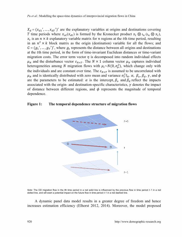
Traditional gravity or spatial interaction models focus on the impacts of origin- anddestination-specific characteristics and the distance-decay effect on observed flows(Sen and Smith 1995; Mátyás 1997). Given this starting point, this study considerstemporal dependence between adjacent time periods. For simplicity, we assume thatmigration flows in a given time period are dependent only on the immediate past periodvalues, regardless of subsequent periods, as shown in Figure 1.

Introducing a first-order time lag of the dependent variable into the traditionalgravity model allows us to determine a dynamic panel data model for migration flowsas shown in Equation (1) (Parent and LeSage 2010, 2012):

= + × + + + + ,= + × , (1)

where = ( , … , ) consists of time periods of migration flows and = ( , … , ) is an ´ 1 ( = ) column vector of regional gross flows

constructed by stacking the columns of the × flow matrix for n regions at the thtime period; = ( , … , ) represents the first-order time lag of in the samemanner; × is an × 1 column vector of ones; = ( , … , ) and




= ( , … , ) are the explanatory variables at origins and destinations covering time periods where ( ) is formed by the Kronecker product ⊗ ( ⊗ ), is an × explanatory variable matrix for regions at the th time period, resulting

in an × block matrix as the origin (destination) variable for all the flows; and = ( , … , ) , where represents the distance between all origins and destinations

at the th time period, in the form of time-invariant Euclidean distances or time-variantmigration costs. The error term vector is decomposed into random individual effects

and the disturbance vector × . The × 1 column vector captures individualheterogeneities among migration flows with ~ (0, ), which change only withthe individuals and are constant over time. The × is assumed to be uncorrelated with

and is identically distributed with zero mean and variance . , , , , andare the parameters to be estimated: is the intercept, and reflect the impactsassociated with the origin- and destination-specific characteristics, denotes the impactof distance between different regions, and represents the magnitude of temporaldependence.

Figure 1: The temporal dependence structure of migration flows

Note: The OD migration flow in the tth time period in a red solid line is influenced by the previous flow in time period t-1 in a reddotted line, and will exert a potential impact on the future flow in time period t+1 in a red dashed line.

A dynamic panel data model results in a greater degree of freedom and henceincreases estimation efficiency (Elhorst 2012, 2014). Moreover, the model proposed




here accounts for more complicated temporal dependence and individual effects thanthe conventional gravity model can capture.

3.2 Spatial dynamic panel data model

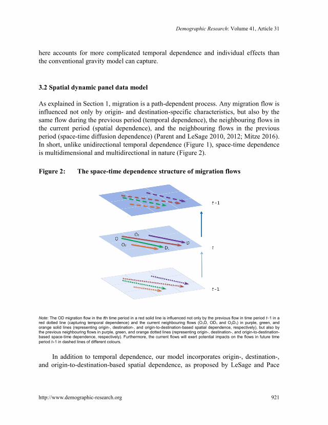
As explained in Section 1, migration is a path-dependent process. Any migration flow isinfluenced not only by origin- and destination-specific characteristics, but also by thesame flow during the previous period (temporal dependence), the neighbouring flows inthe current period (spatial dependence), and the neighbouring flows in the previousperiod (space-time diffusion dependence) (Parent and LeSage 2010, 2012; Mitze 2016).In short, unlike unidirectional temporal dependence (Figure 1), space-time dependenceis multidimensional and multidirectional in nature (Figure 2).

Figure 2: The space-time dependence structure of migration flows

Note: The OD migration flow in the tth time period in a red solid line is influenced not only by the previous flow in time period t-1 in ared dotted line (capturing temporal dependence) and the current neighbouring flows (O1D, OD1 and O2D1) in purple, green, andorange solid lines (representing origin-, destination-, and origin-to-destination-based spatial dependence, respectively), but also bythe previous neighbouring flows in purple, green, and orange dotted lines (representing origin-, destination-, and origin-to-destination-based space-time dependence, respectively). Furthermore, the current flows will exert potential impacts on the flows in future timeperiod t+1 in dashed lines of different colours.

In addition to temporal dependence, our model incorporates origin-, destination-,and origin-to-destination-based spatial dependence, as proposed by LeSage and Pace




(2008, 2009). Assuming is the × spatial weight matrix with zeros on thediagonal, these three types of spatial dependence are defined by the correspondingnetwork weight matrices , , and : = ⊗ , = ⊗ , and =

⊗ (Chun 2008; LeSage and Pace 2008, 2009; LeSage and Llano 2013; Griffith,Fischer, and LeSage 2017).

Based on the spatial dependence of migration flows, we then define another threetypes of space-time diffusion dependence. If a migration flow in a given time period isinfluenced by flows from neighbouring origins to the same destination in the timeperiod immediately preceding it, this can be understood as origin-based space-timedependence. Similarly, destination- and origin-to-destination-based space-timedependence of migration flows can be accordingly defined.

We now extend the general dynamic panel data model with the above spatialdependence and space-time diffusion dependence to derive a spatial dynamic panel datamodel of migration flows (Equation 2):

= ( ⊗ ) + ( ⊗ ) + ( ⊗ ) + + ( ⊗ )+ ( ⊗ ) + ( ⊗ ) + × + ++ + ,

= + × , (2)

where is the -dimensional identity matrix; the Kronecker products ⊗ , ⊗, and ⊗ represent the space-time weight matrices for all migration flows over

time periods; ( ⊗ ) , ( ⊗ ) , and ( ⊗ ) , accordingly, representorigin-, destination-, and origin-to-destination-based spatial lags of migration flows incorresponding time periods; ( ⊗ ) , ( ⊗ ) , and ( ⊗ )represent origin-, destination-, and origin-to-destination-based space-time lags ofmigration flows. Like the scalar parameter of temporal dependence, ( , , ) and( , , ) measure the strength of the spatial dependence and space-time diffusiondependence, respectively.

This study adopts the Bayesian Markov chain Monte Carlo (MCMC) samplingmethod to estimate the associated parameters, thus avoiding multidimensionalnumerical integration in maximum likelihood (ML) or quasi-maximum likelihood(QML) methods (Chib and Carlin 1999; LeSage and Pace 2009; Elhorst 2010, 2012,2014). Specifically, we use Bayesian updating schemes based on the joint posteriordistribution of the parameters of interest in the manner of sampling from their posteriordistributions (Bhargava and Sargan 1983; Parent and LeSage 2010, 2012; LeSage2014). The joint posterior distribution is derived as follows:




, , , , , , , , , , , , ∝ ( |Υ, , , , , )(Υ) ( ) ( ) ( ) ( ), (3)

where Υ = ( , , , ), = ( , , ), and = ( , , ); ( | ⋅) representsthe likelihood function; and (⋅) represents the prior distribution of each parameter.

The samples drawn from the set of conditional posterior distributions by theMCMC sampling method are used to estimate the associated parameters and theirsignificance. The specific MCMC sampling and updating scheme for the spatialdynamic panel model are presented in the Appendix.

3.3 Interpreting the space-time effects of migration processes

For a spatial dynamic panel data model, a change in regional characteristics not onlyhas a direct influence on the outflows and inflows from and to this region, but also hasan indirect effect on the flows to and from other regions in the migration network overspace and time. Therefore, there is a need to quantify various responses in the networkfrom a local perspective (Golgher and Voss 2016). Following LeSage and Thomas-Agnan (2015), we extend the scalar summary measures of origin, destination,intraregional, and spillover effects to a space-time context and decompose them intocontemporaneous, short-, and long-term components to reveal the changing impactsover time.

A change in a typical region at any time will potentially bring about transitoryimpacts on the flows during the period + to different degrees. Specifically, totaleffects (TE) are the impacts on all flows in the manner of × partial derivativesshown in Equation (4) (Debarsy, Ertur, and LeSage 2012; LeSage and Thomas-Agnan2015):

=

⎝

⎜⎛

⋮⎠

⎟⎞=

⎝

⎜⎜⎛ ( )/ ( )

( )/ ( )⋮

( )/ ( )⎠

⎟⎟⎞=

⎝

⎜⎛ +

+⋮+ ⎠

⎟⎞,

= (−1) ( ) , (4) = − − − , = −( + + + ),

where B represents the space filter and C the space-time diffusion filter, allowingproducing the true elasticities of different factors after introducing space-time




interactions. is an × matrix of zeros with the th column equal to , and isan × matrix of zeros with the th row equal to ( = 1,… , ). Thus, the rows of thematrix ( ( )/ ( )) record the impacts on inflows to region , and its columnsrecord the impacts on outflows from region . That is, each element corresponds to thechange of different flows concerning region in detail.

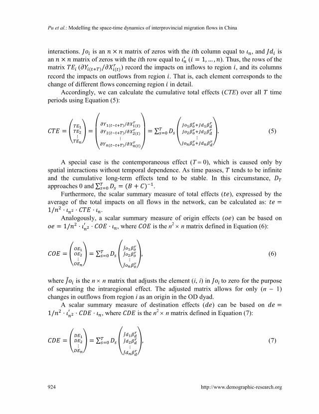
Accordingly, we can calculate the cumulative total effects (CTE) over all timeperiods using Equation (5):

=⋮

=

⎝

⎜⎛ ( ~ )/ ( )

( ~ )/ ( )⋮

( ~ )/ ( )⎠

⎟⎞= ∑

⋮. (5)

A special case is the contemporaneous effect (T = 0), which is caused only byspatial interactions without temporal dependence. As time passes, tends to be infiniteand the cumulative long-term effects tend to be stable. In this circumstance,approaches 0 and ∑ = ( + ) .

Furthermore, the scalar summary measure of total effects ( ), expressed by theaverage of the total impacts on all flows in the network, can be calculated as: =1/ ⋅ ⋅ ⋅ .

Analogously, a scalar summary measure of origin effects ( ) can be based on= 1/ ⋅ ⋅ ⋅ , where is the n2 ´ n matrix defined in Equation (6):

=⋮

= ∑⋮

, (6)

where is the n ´ n matrix that adjusts the element (i, i) in to zero for the purposeof separating the intraregional effect. The adjusted matrix allows for only (n - 1)changes in outflows from region i as an origin in the OD dyad.

A scalar summary measure of destination effects ( ) can be based on =1/ ⋅ ⋅ ⋅ , where is the n2 ´ n matrix defined in Equation (7):

=⋮

= ∑⋮

, (7)




where is the n ´ n matrix that adjusts the element (i, i) in to zero without theintraregional effect. This matrix allows for only (n - 1) changes in inflows to region i asa destination.

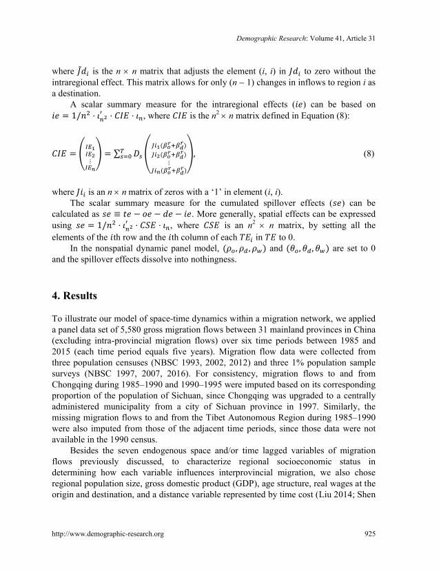
A scalar summary measure for the intraregional effects ( ) can be based on= 1/ ⋅ ⋅ ⋅ , where is the n2 ´ n matrix defined in Equation (8):

=⋮

= ∑( )( )

⋮( )

, (8)

where is an n ´ n matrix of zeros with a ‘1’ in element (i, i).The scalar summary measure for the cumulated spillover effects ( ) can be

calculated as ≡ − − − . More generally, spatial effects can be expressedusing = 1/ ⋅ ⋅ ⋅ , where is an n2 ´ n matrix, by setting all theelements of the th row and the th column of each in to 0.

In the nonspatial dynamic panel model, ( , , ) and ( , , ) are set to 0and the spillover effects dissolve into nothingness.

4. Results

To illustrate our model of space-time dynamics within a migration network, we applieda panel data set of 5,580 gross migration flows between 31 mainland provinces in China(excluding intra-provincial migration flows) over six time periods between 1985 and2015 (each time period equals five years). Migration flow data were collected fromthree population censuses (NBSC 1993, 2002, 2012) and three 1% population samplesurveys (NBSC 1997, 2007, 2016). For consistency, migration flows to and fromChongqing during 1985–1990 and 1990–1995 were imputed based on its correspondingproportion of the population of Sichuan, since Chongqing was upgraded to a centrallyadministered municipality from a city of Sichuan province in 1997. Similarly, themissing migration flows to and from the Tibet Autonomous Region during 1985–1990were also imputed from those of the adjacent time periods, since those data were notavailable in the 1990 census.

Besides the seven endogenous space and/or time lagged variables of migrationflows previously discussed, to characterize regional socioeconomic status indetermining how each variable influences interprovincial migration, we also choseregional population size, gross domestic product (GDP), age structure, real wages at theorigin and destination, and a distance variable represented by time cost (Liu 2014; Shen




2016, 2017). Population size, as a typical gravity variable, has been demonstrated aseffective in driving continued migration flows in China since the late 1970s (Fan 2005).The signs of population size at the origin and destination are expected to be positive,indicating push-pull forces between origins and destinations. GDP at the origin anddestination is used to test the impact of regional economic disparity on stimulatingmigration flows. The expected signs of GDP at the origin and destination are negativeand positive, respectively, suggesting people will move from a relatively poor region toa developed one. Age structure, measured by the proportion of working-age population(ages 15-64), reflects the predominance of labour migration. According to the 2015 1%population survey, labour population accounted for more than 85% of migrants duringthe 2010-2015 period (NBSC 2016). The signs of age structure at the origin anddestination are expected to be positive and negative, respectively, indicating migrantsare moving from labour-supplying regions to labour-demanding ones. Real wages as ameasure of regional economic opportunity are the main motivation for mobility. Weexpect that the signs of real wages at the origin and destination are opposite, meaningthat people will move to a region with higher income from a region with lower income.Compared with the constant railway distance, travel time can reflect improvement intransportation infrastructure. A negative decay effect of time distance is expected.

We use a log transformation of both dependent variable and explanatory variablesto interpret the space-time effects as elasticities. To avoid the endogeneity problem, welagged the dependent variable and explanatory variables by five years (LeSage and Pace2008; Patuelli and Arbia 2016). Thus, the lagged migration flows at the initial period(1985-1990) were taken from the 1987 1% population sample survey (NBSC 1988),while data on regional population size, GDP, the proportion of labour force population,and real wages were collected from the China Statistical Yearbook on the first year oftheir corresponding periods (NBSC 1986, 1991, 1996, 2001, 2006, 2011). Theminimum travel time by railway was collected from the China Railway Timetable at thesame base year as the other exogenous explanatory variables (TBMR 1985, 1990, 1995,2000, 2005, 2010). To check for the problem of potential multicollinearity, we calculatethe variance inflation factor (VIF) for all variables (under 2.50), indicating no seriousmulticollinearity in our model. Table 1 describes these explanatory variables in detail.

We construct the spatial weight matrix based on the first-order contiguity,reflecting whether a common boundary exists between two provinces, denoted by 0or 1. Since Hainan province is an island that once belonged to Guangdong province, wedesignate Guangdong as its neighbour. The spatial weight matrix W is then row-normalized to produce three different network weight matrices , , and . Inpractice, we remove the diagonal elements from , , and to derive the ×matrices , , and ( = × ( − 1)) without considering intraregional flows.Different specifications of the spatial weight matrix have little impact on the subsequent




estimates and inferences, consistent with LeSage and Pace (2014), and hence we focuson the results from the first-order contiguity matrix.

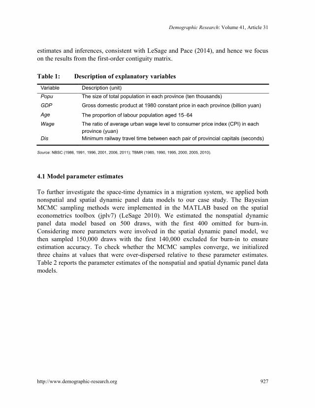
Table 1: Description of explanatory variables

Variable Description (unit)Popu The size of total population in each province (ten thousands)

GDP Gross domestic product at 1980 constant price in each province (billion yuan)

Age The proportion of labour population aged 15-64

Wage The ratio of average urban wage level to consumer price index (CPI) in eachprovince (yuan)

Dis Minimum railway travel time between each pair of provincial capitals (seconds)

Source: NBSC (1986, 1991, 1996, 2001, 2006, 2011); TBMR (1985, 1990, 1995, 2000, 2005, 2010).

4.1 Model parameter estimates

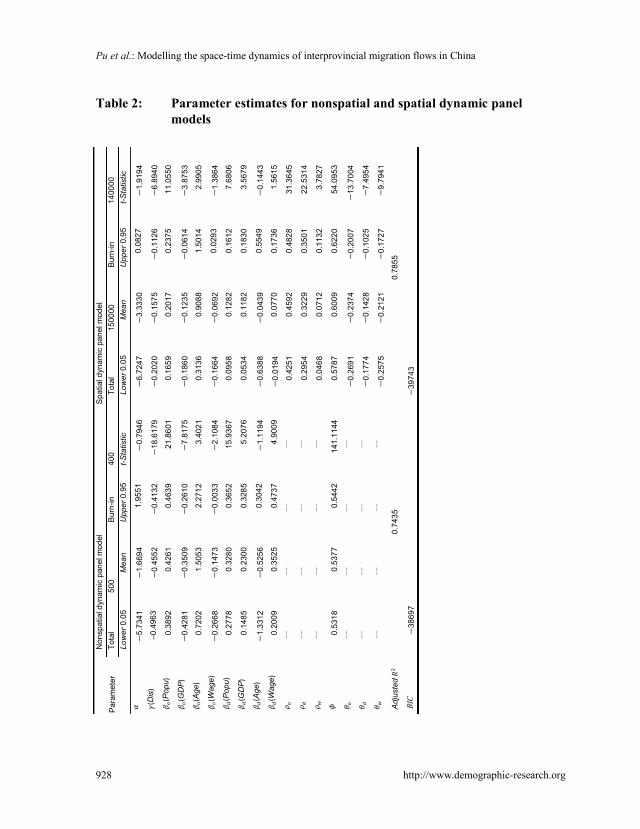
To further investigate the space-time dynamics in a migration system, we applied bothnonspatial and spatial dynamic panel data models to our case study. The BayesianMCMC sampling methods were implemented in the MATLAB based on the spatialeconometrics toolbox (jplv7) (LeSage 2010). We estimated the nonspatial dynamicpanel data model based on 500 draws, with the first 400 omitted for burn-in.Considering more parameters were involved in the spatial dynamic panel model, wethen sampled 150,000 draws with the first 140,000 excluded for burn-in to ensureestimation accuracy. To check whether the MCMC samples converge, we initializedthree chains at values that were over-dispersed relative to these parameter estimates.Table 2 reports the parameter estimates of the nonspatial and spatial dynamic panel datamodels.




Table 2: Parameter estimates for nonspatial and spatial dynamic panelmodels

Par

amet

erN

onsp

atia

l dyn

amic

pan

el m

odel

Spa

tial d

ynam

ic p

anel

mod

elTo

tal

500

Bur

n-in

400

Tota

l15

0000

Bur

n-in

1400

00Lo

wer

0.05

Mea

nU

pper

0.95

t-Sta

tistic

Low

er0.

05M

ean

Upp

er0.

95t-S

tatis

tic

-5.7

341

-1.6

694

1.95

51-0

.794

6-6

.724

7-3

.333

00.

0827

-1.9

194

(Dis)

‒0.4

963

-0.4

552

-0.4

132

-18.

6179

-0.2

020

-0.1

575

-0.1

126

-6.8

940

(Pop

u)0.

3892

0.42

610.

4639

21.8

601

0.16

590.

2017

0.23

7511

.055

0(G

DP)

-0.4

281

-0.3

509

-0.2

610

-7.8

175

-0.1

860

-0.1

235

-0.0

614

-3.8

753

(Age

)0.

7202

1.50

532.

2712

3.40

210.

3136

0.90

881.

5014

2.99

05(W

age)

-0.2

668

-0.1

473

-0.0

033

-2.1

084

-0.1

664

-0.0

692

0.02

93-1

.386

4(P

opu)

0.27

780.

3280

0.36

5215

.936

70.

0958

0.12

820.

1612

7.68

06(G

DP)

0.14

850.

2300

0.32

855.

2076

0.05

340.

1182

0.18

303.

5679

(Age

)-1

.331

2-0

.525

60.

3042

-1.1

194

-0.6

388

-0.0

439

0.55

49-0

.144

3(W

age)

0.20

090.

3525

0.47

374.

9009

-0.0

194

0.07

700.

1736

1.56

15--

----

--0.

4251

0.45

920.

4828

31.3

645

----

----

0.29

540.

3229

0.35

0122

.531

4--

----

--0.

0468

0.07

120.

1132

3.78

27

0.53

180.

5377

0.54

4214

1.11

440.

5787

0.60

090.

6220

54.0

953

----

----

-0.2

691

-0.2

374

-0.2

007

-13.

7004

----

----

-0.1

774

-0.1

428

-0.1

025

-7.4

954

----

----

-0.2

575

-0.2

121

-0.1

727

-9.7

941

Adj

uste

d0.

7435

0.78

55

BIC

-386

97-3

9743




In general, the spatial dynamic panel data model is superior to the nonspatial onein characterizing the Chinese interprovincial migration process during 1985-2015, asseen by its smaller BIC (Bayesian Information Criterion) value. Furthermore, Chineseinterprovincial migration is a path-dependent process, as demonstrated by the fact thattemporal, spatial, and space-time diffusion dependencies are significantly different fromzero. The significant and positive temporal dependence ( ) indicates that past migrantstend to produce future sustained outflows and inflows. In China, migration flows areusually dependent on social linkages, such as relying on family members, friends, orfellow-townspeople for job opportunities (Liu 2014). Even if an entire family moves,their migration process is often unsynchronized. It is the positive network externalitiesthat make subsequent migrants follow the path blazed by the pioneers, giving rise tostrong temporal dependence during migration processes (Epstein 2008). Surprisingly,temporal dependence has been strengthened by including space-time interactions in thespatial dynamic panel data model, rather than the contrary, reflecting networkexternalities’ possible interaction with herd effects.

The significant and positive spatial dependence parameters (ro, rd, and rw) cancorroborate the existence of herd effects during the development of migration flows(Epstein 2008). The origin-, destination-, and origin-to-destination-based spatialdependencies represent three different but complementary migration paths. Specifically,the origin-based path implies that migration flows from the origin to the destinationmay promote outflows from surrounding origins to the same destination. Similarly,migration flows from the origin (or neighbouring origins) to neighbouring destinationsare also enhanced, as implied by the destination-based (or origin-to-destination-based)path. Comparatively, the origin-based path dominates the other two; the largest spatialdependence (ro = 0.4592) is further supported by the fact that origins with strongoutflows are mainly located in China’s central and western regions. Like the time decayeffect, the strength of origin-, destination-, and origin-to-destination-based spatialdependences of less than 1 further corroborates the distance-decay effects over space.

Mutual space-time interactions have negative diffusion effects on migration flows,as reported by the significant and negative parameters ( , , and ). The origin-,destination-, and origin-to-destination-based space-time paths are exerting oppositeroles compared with those three migration paths across space. In other words, if thenumber of migration flows from an origin to a destination at one point in timeincreases, the flows departing from the neighbouring origins to the same destinationduring the next time period will decrease. Similarly, the migration flows from oneorigin (or neighbouring origin regions) to neighbouring destinations in the next periodwill also decrease. Among these space-time paths the flows along the origin-basedspace-time path will decrease sharply due to the coexistence of herd and networkeffects, evidenced by the smallest space-time parameter (qo = -0.2374). This




phenomenon fully reflects the self-adjustment and adaptability of a complex migrationsystem, which involves much more complicated processes than the nonspatial modelsuggests.

Distance, as measured by minimum railway travel time, has significant andnegative effects, as expected. Notably, the distance-decay effect in the spatial dynamicpanel data model is significantly reduced compared with that in the nonspatial model,since spatial dependence can play a role similar to that of distance (LeSage andThomas-Agnan 2015). Although the rapid progress of transportation technology hasgreatly facilitated migration activity, longer distances and higher time costs still restrictpeople’s aspirations to migrate, as does the relative scarcity of information about distantregions (Huff and Jenks 2015).

The coefficient estimates of explanatory variables in the spatial dynamic paneldata model should not be directly interpreted as partial derivative impacts of regionalfactors on migration flows. To better understand the space-time dynamics indetermining interprovincial migration processes in China, we perform a comprehensivequantitative analysis by calculating various space-time effects of explanatory variablesand drawing valid inferences about their statistical significance.

4.2 Analysis of space-time effects

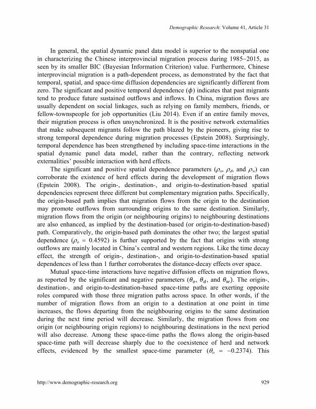
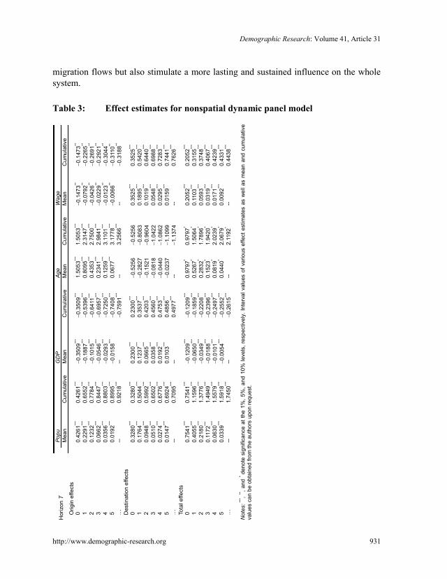
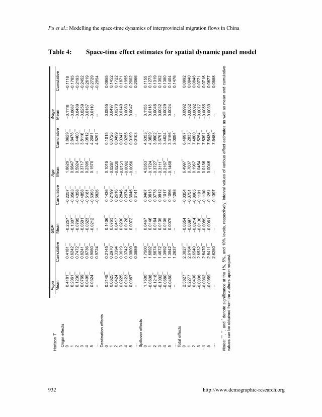
Tables 3 and 4 show various effect estimates of regional population size, GDP, agestructure, and real wages in the nonspatial and spatial dynamic panel data models,respectively. The rows labelled ‘0’ represent the immediate responses of migrationflows to changes in regional characteristics in terms of contemporaneous effects. Thefollowing rows labelled between ‘1’ and ‘5’ capture the disaggregated period-by-periodimpacts on the follow-on migration flows at different time periods. The last rowslabelled ‘…’ reflect the cumulative long-term effects. The columns labelled ‘Mean’record the means of the transitory period-by-period effects and the columns labelled‘Cumulative’ the accumulated effects from the initial period to the current period.

Influenced by the temporal dependence and distance-decaying effects, variousperiod-by-period effects are gradually reduced to zero over time, while thecorresponding cumulative effects tend to approach their long-term effects in the future.This phenomenon conforms to the evolution of a migration system in reality. Theintroduction of space-time interactions in the spatial dynamic panel data model bringsabout profound changes in all kinds of effects. Overall, the role of regional factors issignificantly extended and deepened in the spatial model, reflecting that space-timeinteractions not only promote closer connections between different interprovincial




migration flows but also stimulate a more lasting and sustained influence on the wholesystem.

Table 3: Effect estimates for nonspatial dynamic panel model

Hor

izon

TP

opu

GD

PAg

eW

age

Mea

nC

umul

ativ

eM

ean

Cum

ulat

ive

Mea

nC

umul

ativ

eM

ean

Cum

ulat

ive

Orig

in e

ffect

s0

0.42

61**

*0.

4261

***

-0.3

509**

*-0

.350

9***

1.50

53**

*1.

5053

***

-0.1

473**

-0.1

473**

10.

2291

***

0.65

52**

*-0

.188

7***

-0.5

396**

*0.

8095

***

2.31

47**

*-0

.079

2**-0

.226

5**

20.

1232

***

0.77

84**

*-0

.101

5***

-0.6

411**

*0.

4353

***

2.75

00**

*-0

.042

6**-0

.269

1**

30.

0662

***

0.84

47**

*-0

.054

6***

-0.6

957**

*0.

2341

***

2.98

41**

*-0

.022

9**-0

.292

1**

40.

0356

***

0.88

03**

*-0

.029

3***

-0.7

250**

*0.

1259

***

3.11

01**

*-0

.012

3**-0

.304

4**

50.

0192

***

0.89

95**

*-0

.015

8***

-0.7

408**

*0.

0677

***

3.17

78**

*-0

.006

6**-0

.311

0**

…--

0.92

18**

*--

-0.7

591**

*--

3.25

66**

*--

-0.3

188**

Des

tinat

ion

effe

cts

00.

3280

***

0.32

80**

*0.

2300

***

0.23

00**

*-0

.525

6-0

.525

60.

3525

***

0.35

25**

*

10.

1764

***

0.50

44**

*0.

1237

***

0.35

37**

*-0

.282

7-0

.808

30.

1895

***

0.54

20**

*

20.

0948

***

0.59

92**

*0.

0665

***

0.42

03**

*-0

.152

1-0

.960

40.

1019

***

0.64

40**

*

30.

0510

***

0.65

02**

*0.

0358

***

0.45

60**

*-0

.081

8-1

.042

20.

0548

***

0.69

88**

*

40.

0274

***

0.67

76**

*0.

0192

***

0.47

53**

*-0

.044

0-1

.086

20.

0295

***

0.72

83**

*

50.

0147

***

0.69

24**

*0.

0103

***

0.48

56**

*-0

.023

7-1

.109

90.

0159

***

0.74

41**

*

…--

0.70

95**

*--

0.49

77**

*--

-1.1

374

--0.

7626

***

Tota

l effe

cts

00.

7541

***

0.75

41**

*-0

.120

9***

-0.1

209**

*0.

9797

*0.

9797

*0.

2052

***

0.20

52**

*

10.

4055

***

1.15

96**

*-0

.065

0***

-0.1

859**

*0.

5267

*1.

5064

*0.

1103

***

0.31

55**

*

20.

2180

***

1.37

76**

*-0

.034

9***

-0.2

208**

*0.

2832

*1.

7896

*0.

0593

***

0.37

48**

*

30.

1172

***

1.49

49**

*-0

.018

8***

-0.2

396**

*0.

1523

*1.

9420

*0.

0319

***

0.40

67**

*

40.

0630

***

1.55

79**

*-0

.010

1***

-0.2

497**

*0.

0819

*2.

0239

*0.

0171

***

0.42

39**

*

50.

0339

***

1.59

18**

*-0

.005

4***

-0.2

552**

*0.

0440

*2.

0679

*0.

0092

***

0.43

31**

*

…--

1.74

50**

*--

-0.2

615**

*--

2.11

92*

--0.

4438

***

Not

es:**

* ,**, a

nd*de

note

sig

nific

ance

at t

he 1

%, 5

%, a

nd 1

0% le

vels

, res

pect

ivel

y. In

terv

al v

alue

s of

var

ious

effe

ct e

stim

ates

as

wel

l as

mea

n an

d cu

mul

ativ

eva

lues

can

be

obta

ined

from

the

auth

ors

upon

requ

est.




Table 4: Space-time effect estimates for spatial dynamic panel modelH

oriz

onT

Pop

uG

DP

Age

Wag

eM

ean

Cum

ulat

ive

Mea

nC

umul

ativ

eM

ean

Cum

ulat

ive

Mea

nC

umul

ativ

eO

rigin

effe

cts

00.

4181

***

0.41

81**

*-0

.225

7***

-0.2

257**

*1.

8629

***

1.86

29**

*-0

.111

8-0

.111

81

0.20

61**

*0.

6242

***

-0.1

307**

*-0

.356

3***

0.98

47**

*2.

8476

***

-0.0

667

-0.1

785

20.

1230

***

0.74

72**

*-0

.079

5***

-0.4

358**

*0.

5924

***

3.44

00**

*-0

.040

9-0

.219

33

0.07

69**

*0.

8241

***

-0.0

501**

*-0

.485

8***

0.37

17**

*3.

8116

***

-0.0

259

-0.2

452

40.

0495

***

0.87

36**

*-0

.032

3***

-0.5

181**

*0.

2395

***

4.05

12**

*-0

.016

7-0

.261

95

0.03

24**

*0.

9060

***

-0.0

212**

*-0

.539

3***

0.15

70**

*4.

2081

***

-0.0

110

-0.2

729

…--

0.97

24**

*--

-0.5

826**

*--

4.52

91**

*--

-0.2

954

Des

tinat

ion

effe

cts

00.

2145

***

0.21

45**

*0.

1436

***

0.14

36**

*0.

1015

0.10

150.

0955

0.09

551

0.08

25**

*0.

2970

***

0.07

63**

*0.

2199

***

-0.0

287

0.07

280.

0497

0.14

522

0.04

24**

*0.

3394

***

0.04

17**

*0.

2616

***

-0.0

230

0.04

990.

0270

0.17

223

0.02

25**

*0.

3619

***

0.02

30**

*0.

2846

***

-0.0

151

0.03

470.

0149

0.18

714

0.01

23**

*0.

3742

***

0.01

28**

*0.

2974

***

-0.0

092

0.02

550.

0083

0.19

555

0.00

67**

*0.

3809

***

0.00

72**

*0.

3046

***

-0.0

056

0.01

990.

0047

0.20

02…

--0.

3889

***

--0.

3141

***

--0.

0103

--0.

2066

Spi

llove

reffe

cts

01.

7500

***

1.75

00**

*0.

0467

0.04

674.

5353

**4.

5353

**0.

1155

0.11

551

-0.0

608

1.68

92**

*0.

0146

0.06

13-0

.172

44.

3629

*0.

0118

0.12

732

-0.1

218**

1.56

74**

*0.

0164

0.07

78-0

.372

7*3.

9902

*0.

0046

0.13

193

-0.1

002**

*1.

4672

***

0.01

350.

0912

-0.3

111**

3.67

91*

0.00

320.

1352

4-0

.068

0***

1.39

92**

*0.

0105

0.10

17-0

.216

7***

3.46

24*

0.00

290.

1380

5-0

.045

0***

1.35

42**

*0.

0079

0.10

96-0

.146

8***

3.31

56*

0.00

240.

1404

…--

1.26

37**

*--

0.12

88--

3.00

94*

--0.

1476

Tota

l effe

cts

02.

3827

***

2.38

27**

*-0

.035

4-0

.035

46.

4997

**6.

4997

**0.

0992

0.09

921

0.22

772.

6104

***

-0.0

397

-0.0

751

0.78

377.

2833

**-0

.005

20.

0940

20.

0436

2.65

40**

*-0

.021

4**-0

.096

50.

1967

7.48

00**

-0.0

092

0.08

483

-0.0

008

2.65

32**

*-0

.013

6***

-0.1

101

0.04

547.

5254

**-0

.007

70.

0771

4-0

.006

22.

6470

***

-0.0

089**

*-0

.119

00.

0136

7.53

91**

-0.0

055

0.07

165

-0.0

059**

*2.

6411

***

-0.0

061**

*-0

.125

10.

0046

7.54

36**

-0.0

039

0.06

77…

--2.

6250

***

---0

.139

7--

7.54

88**

--0.

0588

Not

es: *

**,**

, and

*de

note

sig

nific

ance

at t

he 1

%, 5

%, a

nd 1

0% le

vels

, res

pect

ivel

y. In

terv

al v

alue

s of

var

ious

effe

ct e

stim

ates

as

wel

l as

mea

n an

d cu

mul

ativ

eva

lues

can

be

obta

ined

from

the

auth

ors

upon

requ

est.




4.2.1 Population size

Population size is often chosen as the basic explanatory variable to characterize regionalmass in traditional gravity models (Zipf 1946; Stillwell 2008). Migration flows betweenorigins and destinations are positively proportional to their population sizes if othervariables are held constant. Tables 3 and 4 show that, as hypothesized, the origin anddestination effects of population size are significantly positive, exerting strong push andpull forces on interprovincial migration in China from 1985 to 2015. In addition, thecumulative origin and destination effects of population size continue to increase overtime, indicating that changes in regional population have profound impacts onmigration flows. The origin effects of population size are larger than the correspondingdestination effects, reflecting the fact that the pressure from large populations is muchstronger than their agglomeration effects during the migration process. In a typicalregion, a 1% increase in population size produces 0.42% more outflow during the sameperiod. As time passes, transitory responses remain significantly positive, eventuallyleading to 0.97% additional outflow over the long term. On the other hand, a 1%increase in population size in a typical region produces 0.21% more inflow during thesame period and 0.39% additional inflow in the long run, less than half of its long-termorigin effect.

More importantly, changes in regional population size also impact the inflows andoutflows to and from other regions through the migration network over time. It is thesecomplex spillover effects that demonstrate the close link between migration flows. Thespatial dynamic panel data model allows us to measure these invisible effects; themagnitude of such effects is beyond our expectations. Specifically, the cumulativespillover effects at different time periods are greater than 1.0, indicating a more rapidincrease of migration flows arising from the same population growth across thenetwork. On average, if a given population size in a typical region increases by 1%, themigration flows between other provinces will increase by 1.75% over the same period,well beyond the increase of outflows and inflows from and to the given region. Thiskind of spillover effect occurring at the same time (herd effect) may cause large flowseven before networks are created, providing a complementary explanation for theformation of migration flows (Epstein 2008). As time passes, negative feedback effectsin the following periods gradually weaken the cumulative network effects andeventually lead to a long-term effect of 1.2637, over two-thirds of its contemporaneouseffect. These negative network externalities are also consistent with the reality that thenumber of immigrants may gradually reduce as the increase in new arrivals results inmore competition for jobs. Declining network effects may help prevent the migrationsystem from becoming out of control.

Total effects, represented by the sum of origin, destination, and spillover effects,reflect broader societal responses to changes in regional population size. The estimates




in Table 4 show that population size has the second largest impact on Chineseinterprovincial migration flows. On average, a 1% increase in regional population in atypical region increases migration flows by 2.38% during the same period and by2.63% over the long term. Although the spillover effects of population may decreaseover time, they are still greater than its origin and destination effects. In other words, wecannot ignore the role of spillover effects in addition to traditional push and pull forceson the formation and development of migration flows.

4.2.2 GDP

Unbalanced regional economic development in China has led to continuing internalmigration flows since the late 1970s (Cai and Wang 2003; Zhu 2003; Fan 2005).Tables 3 and 4 show that regional GDP plays a significant role in causing people tomove between different areas, consistent with the neoclassical migration theory(Sjaastad 1962). The negative origin effects’ inhibiting role is strong during the initialperiod. On average, a 1% increase in regional GDP produces 0.23% less outflow in thesame period (T = 0). As time passes the period-by-period effects decrease but remainsignificant. Over the long run the origin effect of GDP reaches -0.5826, an absolutevalue much larger than that of GDP during the contemporaneous period. In other words,regional economic development tends to reduce migration outflows over time.

As expected, the development of a regional economy attracts more immigrants, asevidenced by the significant and positive destination effects of GDP. On average, a 1%increase in GDP in a typical region attracts 0.14% more inflows during the same periodand 0.08% more inflows during the following period (T = 1). Although the period-by-period effects appear to decay over time, the cumulative effect still reaches 0.3141 overthe long term, twice that of the contemporaneous effect. If we do not consider thespace-time interactions among migration flows (Table 3), most of the destination effectsof GDP tend to be overestimated, thus ignoring the self-adjustment of migrationprocesses.

Regional GDP’s spillover effects are not as significant as its origin and destinationeffects. In other words, the role of regional GDP in generating and attracting migrationflows is mainly limited to the local inflows and outflows associated with the changingregions, exerting less externalities on the other surroundings. However, the positiveperiod-by-period responses of GDP may accumulate to a larger long-term effect.Eventually, a 1% increase in regional GDP in a typical region produces 0.13% moreflows to other provinces throughout the migration system, which is very close to itscontemporaneous destination effect.




Overall, the total effects of regional GDP can help explain the inverted U-shaperelationship between development and migration. After sustained and rapid growth ofinterprovincial migration, China has experienced a declining trend since 2010 (NBSC1993, 1997, 2002, 2007, 2012, 2016). Furthermore, the period-by-period effects ofregional GDP for the contemporaneous time period out to one time horizon (T = 1) arenot significantly different from zero, indicating that development may not necessarilydecrease migration flows. In reality, regional economic development, at least in theinitial time periods, may enhance migration because development enables and inspirespeople to move (Zelinsky 1971, De Haas 2007, 2010b). However, the transitory period-by-period effects of regional GDP are significant from the two time horizons (T = 2) on,reflecting that development does have a lagged decaying effect on migration.

4.2.3 Age structure

The labour force population is the most influential driver of migration flows. Accordingto population censuses and national survey data (NBSC 1993, 1997, 2002, 2007, 2012,2016), migrant workers dominate in the total migration population. From Table 4 wesee that the origin effects of the proportion of working age population are the largest ofall the explanatory variables, consistent with the nonspatial model estimates. Theimpact of a 1% increase in working age population at origin would result in a 1.86%increase in outflows during the same period and eventually a 4.53% outflow increase,more than four times the origin effects of population size. The enhancement of origineffects in the spatial model is the result of feedback effects arising from changes innetwork flows associated with regions neighbouring each OD dyad. The smallmagnitude of destination effects suggests that an increase in the proportion of locallabour population does not significantly attract more foreigners to move in, indicatingthat its agglomeration effects are rather limited.

The spillover effects arising from the increase in the proportion of the labour-forcepopulation are considerable, making a great difference to the evolution of a migrationsystem. Specifically, a 1% increase in the proportion of labour force in a typical regionleads to a 4.54% contemporaneous increase in other flows throughout the network,surpassing its cumulative origin effect in the long run. In practice this increase would bemainly concentrated in areas neighbouring the region where the proportion of labourforce has increased. More strikingly, such period-by-period spillover effects tend to bemore significant over time. It can be reasonably speculated that a change in the regionallabour force market will have a lasting impact on other regions because of thesignificant space-time interactions. In the long run, the spillover effect for a 1%increase in the proportion of labour force in a typical region will produce 3.01% more




flows to other provinces throughout the migration network, making it a remarkabledriving force.

Overall, interprovincial migration flows in China are extremely sensitive to the agestructure of the population. Specifically, if the proportion of working age population ina typical region increases (or decreases) by 1%, there will be an increase (or decrease)of migration flows by 6.50% during the same period and by 7.55% over the long-term.That is, a slight change in the age structure of a regional population will have a greatinfluence on current and future flows, especially in the contemporaneous period. Thissuggests that herd effects may dominate in migration processes, in line with theemployment-oriented long-distance migration trends (Thomas, Gillespie, and Lomax2019).

4.2.4 Real wages

A large number of migration studies indicate that people migrate to seek better jobopportunities and to increase their quality of life (Chi and Voss 2005; Yue et al. 2010;Chen and Wang 2018). Without the consideration of space-time interactions, real wagesdo play a dominant role in the Chinese interprovincial migration process, as evidencedby various effect estimates shown in Table 3. However, this is not the case in the spatialmodel. We can see from Table 4 that the effect estimates of real wages are no longersignificant, reflecting that real wages are not as important as expected in migrationprocesses. These empirical results confirm that migrants are willing to give up higherwages initially, but prefer to move to more prosperous regions over time (Epstein2008).

In practice, real wages express both the income and consumption of urbanresidents. On the one hand, developed regions with higher wage levels also have higherconsumption standards and more survival pressure, reducing these regions’attractiveness to some potential migrants and affecting their migration decisions. On theother hand, remote and border regions with higher wage levels supported by nationalpolicies, such as the Tibet Autonomous Region, are not major destinations in China,going against the general expectation that regions with higher wages attract moremigrants (Liu and Shen 2014). Overall, an increase in real wages reduces localresidents’ motivation to migrate and encourages more people to move in. A balancebetween wage income and living costs is essential for potential migrants’ decision-making. If the quality of life in an area meets their expectations, most residents tend tostay where they live, reflecting the traditional Chinese attitude towards life: ‘happinesslies in contentment’ (Zhi zu chang le).




5. Conclusions

Migration is arguably playing an increasingly important role in regional growth anddevelopment than ever before. To understand the space-time dynamics of complexmigration processes, this study constructs a spatial dynamic panel data model byincorporating temporal, spatial, and space-time diffusion dependencies into traditionalgravity models. Moreover, we decompose origin, destination, and spillover effects intotheir contemporaneous, short-, and long-term components, thereby providing the toolsto quantify the transitory and cumulative responses of migration flows to changes inregional characteristics. We then apply this model to interprovincial migration flowsbetween 31 mainland provinces in China from 1985 to 2015, choosing population size,GDP, age structure, real wages at origin and destination, and railway travel timebetween provincial capitals as explanatory variables. To evaluate the importance ofspace-time interactions, we use a general (nonspatial) dynamic panel data model as abenchmark specification. Finally, we employ Bayesian MCMC procedures to estimatevarious effects and draw valid inferences regarding the mechanisms of Chineseinterprovincial migration processes.

Our empirical results show that the spatial dynamic panel data model is moresuitable for characterizing the path-dependent migration process. Past migrants tend toproduce sustained outflows and inflows, as evidenced by more strong temporaldependence. Moreover, the origin-, destination-, and origin-to-destination-based pathscomplement one another during the generation and development of migration flows, asconfirmed by the significant and positive spatial dependence. Comparatively, theorigin-based path dominates the other two. However, the origin-, destination-, andorigin-to-destination-based space-time paths provide different channels with which toadjust migration flows, as reflected by significant and negative space-time diffusioninteractions. The origin-based space-time path is likely to be the most effective way toadjust the migration system toward an equilibrium state. Migration flows areperpetuated by the inertia of positive temporal and spatial dependence as well as bynegative space-time diffusion dependence.

The disaggregation of origin, destination, and spillover effects over time furtherallows us to investigate the complex space-time dynamics underlying path-dependentmigration processes. First, the development of migration flows in China is verysensitive to the age structure of regional populations, as a reflection of the workforcecomposition. A slight change in the proportion of the workforce will not only have astrong impact on outflows through transitory and cumulative origin effects, but will alsoinfluence other flows through diffusion effects, especially contemporaneous herdeffects. Second, regional population size also plays a prominent role in migrationprocesses. Specifically, the significant and positive spillover effects are much larger




than the sum of origin and destination effects, indicating that herd and networkexternality effects dominate in the migration system. Third, the inverted U-shaperelationship between development and migration can be partly explained by the totaleffects of regional GDP. Finally, the role of real wages in driving migration flows israther weak, suggesting that migrants are willing to give up higher wages initially butprefer prosperous regions in the long run.

The gravity model remains popular within the field of migration studies (O’Kelly2004). Adding space-time components to this model will not only help promotetheoretical, methodological, and empirical aspects of migration modelling, but alsoadvance its application in other spatial interaction modelling areas such astransportation and international and interregional trade. More importantly, temporal,spatial, and space-time dependencies represent inertia in a system: Monitoring andobserving their presence will help us understand the vulnerability and resilience of aregional system (Griffith and Chun 2015). In a rapidly changing society it is of criticalimportance to be able to predict what will happen to a regional migration system undershock, and how to respond. The space-time framework can be applied to forecast futuremigration flows as well as to explain past and present processes (Baltagi, Fingleton, andPirotte 2019).

The spatial dynamic panel approach proposed in this study is a powerful means tounderstand how migration flows respond to regional socioeconomic changes and howspace and time influence migration processes. However, the various coefficient andeffect estimates are computationally expensive because more parameters are involved inthe spatial model: Practical parallel strategies need to be tested. In addition, we onlyconsidered global spillover effects with a dependent variable lagged in both space andtime: Possible local spillover effects can be investigated in a spatial dynamic Durbinpanel model. Furthermore, we ignored model uncertainty in the selection of explanatoryvariables: The Bayesian model averaging method can be further explored with moreregional social, economic, and environmental factors. Overall, to track the complexevolution of a regional migration system in future research, other types of spatial-temporal models for dyadic flow data should be specified, interpreted, and calibrated.

6. Acknowledgements

The authors thank the editors and four anonymous referees for their insightfulcomments and suggestions. This research was supported in part by the National NaturalScience Foundation of China [#41771417].




References

Anselin, L., Le Gallo, J., and Jayet, H. (2008). Spatial panel econometrics. In: Mátyás,L. and Sevestre, P. (eds.). The econometrics of panel data: Fundamentals andrecent developments in theory and practice. Berlin: Springer: 625‒660.doi:10.1007/978-3-540-75892-1_19.

Baláž, V. and Williams, A.M. (2007). Path-dependency and path-creation perspectiveson migration trajectories: The economic experiences of Vietnamese migrants inSlovakia. International Migration 45(2): 37-66. doi:10.1111/j.1468-2435.2007.00403.x.

Baltagi, B.H., Fingleton, B., and Pirotte, A. (2019). A time-space dynamic panel datamodel with spatial moving average errors. Regional Science and UrbanEconomics 76: 13-31. doi:10.1016/j.regsciurbeco.2018.04.013.

Bauer, T., Epstein, G.S., and Gang, I.N. (2007). The influence of stocks and flows onmigrants’ location choices. Research in Labor Economics 26: 199-229.doi:10.1016/S0147-9121(06)26006-0.

Bavaud, F., Kordi, M., and Kaiser, C. (2018). Flow autocorrelation: A dyadic approach.Annals of Regional Science 61(1): 95-111. doi:10.1007/s00168-018-0860-y.

Beenstock, M. and Felsenstein, D. (2019). The econometric analysis of non-stationaryspatial panel data. Switzerland: Springer. doi:10.1007/978-3-030-03614-0.

Bellos, S. and Subasat, T. (2012). Governance and foreign direct investment: A panelgravity model approach. Bulletin of Economic Research 64(4): 565–574.doi:10.1111/j.1467-8586.2010.00370.x.

Bernard, A. (2017). Cohort measures of internal migration: Understanding long-termtrends. Demography 54(6): 2201-2221. doi:10.1007/s13524-017-0626-7.

Bhargava, A. and Sargan, J.D. (1983). Estimating dynamic random effects models frompanel data covering short time periods. Econometrica 51(6): 1635-1659.doi:10.2307/1912110.

Biagi, B., Faggian, A., Rajbhandari, I., and Venhorst, V.A. (2018). New frontiers ininterregional migration research. Cham: Springer International Publishing.doi:10.1007/978-3-319-75886-2.

Bijak, J. (2011). Forecasting international migration in Europe: A Bayesian view.Berlin: Springer. doi:10.1007/978-90-481-8897-0.

https://doi.org/10.1007/978-3-540-75892-1_19

https://doi.org/10.1111/j.1468-2435.2007.00403.x

https://doi.org/10.1111/j.1468-2435.2007.00403.x

https://doi.org/10.1016/j.regsciurbeco.2018.04.013

https://doi.org/10.1016/S0147-9121(06)26006-0

https://doi.org/10.1007/s00168-018-0860-y

https://doi.org/10.1007/978-3-030-03614-0

https://doi.org/10.1111/j.1467-8586.2010.00370.x

https://doi.org/10.1007/s13524-017-0626-7

https://doi.org/10.2307/1912110

https://doi.org/10.1007/978-3-319-75886-2

https://doi.org/10.1007/978-90-481-8897-0




Black, W. (1992). Network autocorrelation in transportation network and flow systems.Geographical Analysis 24(3): 207-222. doi:10.1111/j.1538-4632.1992.tb00262.x.

Cai, F. and Wang, D. (2003). Migration as marketization: What can we learn fromChina’s 2000 census data? China Review 3(2): 73–93.

Chen, J. and Wang, W. (2018). Economic incentives and settlement intentions of ruralmigrants: Evidence from China. Journal of Urban Affairs 41(3): 372–389.doi:10.1080/07352166.2018.1439339.

Chi, G. and Voss, P.R. (2005). Migration decision-making: A hierarchical regressionapproach. Journal of Regional Analysis and Policy 35(2): 11–22.

Chib, S. and Carlin, B.P. (1999). On MCMC sampling in hierarchical longitudinalmodels. Statistics and Computing 9(1): 17-26. doi:10.1023/A:1008853808677.

Chort, I. and de la Ruppelle, M. (2016). Determinants of Mexico–U.S. outward andreturn migration flows: A state-level panel data analysis. Demography 53(5):1453-1476. doi:10.1007/s13524-016-0503-9.

Chun, Y. (2008). Modeling network autocorrelation within migration flows byeigenvector spatial filtering. Journal of Geographical Systems 10(4): 317-344.doi:10.1007/s10109-008-0068-2.

Chun, Y. and Griffith, D. (2011). Modeling network autocorrelation in space–timemigration flow data: An eigenvector spatial filtering approach. Annals of theAssociation of American Geographers 101(3): 523-536. doi:10.1080/00045608.2011.561070.

Church, J. and King, I. (1993). Bilingualism and network externalities. The CanadianJournal of Economics 26(2): 337-345. doi:10.2307/135911.

Crown, D., Jaquet, T., and Faggian, A. (2018). Interregional migration and implicationsfor regional resilience. In: Biagi, B., Faggian, A., Rajbhandari, I., and Venhorst,V.A. (eds.). New frontiers in interregional migration. Cham: SpringerInternational Publishing: 231-252. doi:10.1007/978-3-319-75886-2_11.

Cushing, B. and Poot, J. (2003). Crossing boundaries and borders: Regional scienceadvances in migration modelling. Papers in Regional Science 83(1): 317-338.doi:10.1007/s10110-003-0188-5.

Davidescu, A.A.M., Strat, V.A., Grosu, R.M., and Zgură, I.D. (2017). Determinants ofRomanians’ migration within the European Union: Static and dynamic panelgravity approaches. Amfiteatru Economic 19(46): 621-639.

https://doi.org/10.1111/j.1538-4632.1992.tb00262.x


https://doi.org/10.1080/07352166.2018.1439339

https://doi.org/10.1023/A:1008853808677

https://doi.org/10.1007/s13524-016-0503-9

https://doi.org/10.1007/s10109-008-0068-2

https://doi.org/10.1080/00045608.2011.561070

https://doi.org/10.1080/00045608.2011.561070

https://doi.org/10.2307/135911

https://doi.org/10.1007/978-3-319-75886-2_11

https://doi.org/10.1007/s10110-003-0188-5




De Haas, H. (2007). Turning the tide? Why development will not stop migration.Development and Change 38(5): 819-841. doi:10.1111/j.1467-7660.2007.00435.x.

De Haas, H. (2010a). The internal dynamics of migration processes: A theoreticalinquiry. Journal of Ethnic and Migration Studies 36(10): 1587-1617.doi:10.1080/1369183X.2010.489361.

De Haas, H. (2010b). Migration and development: A theoretical perspective.International Migration Review 44(1): 227-264. doi:10.1111/j.1747-7379.2009.00804.x.

Debarsy, N., Ertur, C., and LeSage, J. P. (2012). Interpreting dynamic space–time paneldata models. Statistical Methodology 9(1): 158-171. doi:10.1016/j.stamet.2011.02.002.

Elhorst, J.P. (2010). Spatial panel data models. In: Fischer, M.M. and Getis, A. (eds.).Handbook of applied spatial analysis: Software tools, methods and applications.Berlin: Springer: 377-407. doi:10.1007/978-3-642-03647-7_19.

Elhorst, J.P. (2012). Dynamic spatial panels: Models, methods and inferences. Journalof Geographical Systems 14(1): 5-28. doi:10.1007/s10109-011-0158-4.

Elhorst, J.P. (2014). Spatial econometrics: From cross-sectional data to spatial panels.London: Springer. doi:10.1007/978-3-642-40340-8.

Epstein, G.S. (2008). Herd and network effects in migration decision-making. Journalof Ethnic and Migration Studies 34(4): 567-583. doi:10.1080/13691830801961597.

Etzo, I. (2011). The determinants of the recent interregional migration flows in Italy: Apanel data analysis. Journal of Regional Science 51(5): 948–966.doi:10.1111/j.1467-9787.2011.00730.x.

Fan, C.C. (2005). Modeling interprovincial migration in China, 1985–2000. EurasianGeography and Economics 46(3): 165-184. doi:10.2747/1538-7216.46.3.165.

Fotheringham, A.S. (1991). Migration and spatial structure: The development of thecompeting destinations model. In: Stillwell, J. and Congdon, P. (eds.). Migrationmodels: Macro and micro approaches. London: Belhaven Press: 57-72.

Golgher, A.B. and Voss, P.R. (2016). How to interpret the coefficients of spatialmodels: Spillovers, direct and indirect effects? Spatial Demography 4(3):175-205. doi:10.1007/s40980-015-0016-y.

https://doi.org/10.1111/j.1467-7660.2007.00435.x

https://doi.org/10.1111/j.1467-7660.2007.00435.x

https://doi.org/10.1080/1369183X.2010.489361

https://doi.org/10.1111/j.1747-7379.2009.00804.x

https://doi.org/10.1111/j.1747-7379.2009.00804.x

https://doi.org/10.1016/j.stamet.2011.02.002

https://doi.org/10.1016/j.stamet.2011.02.002

https://doi.org/10.1007/978-3-642-03647-7_19

https://doi.org/10.1007/s10109-011-0158-4

https://doi.org/10.1007/978-3-642-40340-8

https://doi.org/10.1080/13691830801961597

https://doi.org/10.1080/13691830801961597

https://doi.org/10.1111/j.1467-9787.2011.00730.x

https://doi.org/10.2747/1538-7216.46.3.165

https://doi.org/10.1007/s40980-015-0016-y




Greenwood, M.J. (1969). An analysis of the determinants of geographic labor mobilityin the United States. Review of Economics and Statistics 51(2): 189-194.doi:10.2307/1926728.

Greenwood, M.J. (1970). Lagged response in the decision to migrate. Journal ofRegional Science 10(3): 375-384. doi:10.1111/j.1467-9787.1970.tb00059.x.

Griffith, D.A. (2009). Spatial autocorrelation in spatial interaction: Complexity-to-simplicity in journey-to-work flows. In: Reggiani, A. and Nijkanmp, P. (eds.).Complexity and spatial networks. Berlin: Springer: 221-237. doi:10.1007/978-3-642-01554-0_16.

Griffith, D.A. and Chun, Y. (2015). Spatial autocorrelation in spatial interactionsmodels: Geographic scale and resolution implication for network resilience andvulnerability. Networks and Spatial Economics 15(2): 337-365. doi:10.1007/s11067-014-9256-4.

Griffith, D.A. and Fischer, M.M. (2013). Constrained variants of the gravity model andspatial dependence: Model specification and estimation issues. Journal ofGeographical Systems 15(3): 291-317. doi:10.1007/s10109-013-0182-7.

Griffith, D.A., Fischer, M.M., and LeSage, J.P. (2017). The spatial autocorrelationproblem in spatial interaction modeling: A comparison of two commonsolutions. Letters in Spatial and Resource Sciences 10(1): 75-86. doi:10.1007/s12076-016-0172-8.

Griffith, D.A. and Jones, K. (1980). Explorations into the relationships between spatialstructure and spatial interaction. Environment and Planning A 12(2): 187-201.doi:10.1068/a120187.

Huff, D.L. and Jenks, G.F. (2015). A graphic interpretation of the friction of distance ingravity models. Annals of the Association of American Geographers 58(4):814-824. doi:10.1111/j.1467-8306.1968.tb01670.x.

Kau, J.B. and Sirmans, C.F. (1979). A recursive model of the spatial allocation ofmigrants. Journal of Regional Science 19(1): 47-56. doi:10.1111/j.1467-9787.1979.tb00570.x.

Laber, G. (1972). Lagged response in the decision to migrate: A comment. Journal ofRegional Science 12(2): 307-310. doi:10.1111/j.1467-9787.1972.tb00352.x.

Lamonica, G.R. and Zagaglia, B. (2013). The determinants of internal mobility in Italy,1995-2006: A comparison of Italians and resident foreigners. DemographicResearch 29(16): 407-440. doi:10.4054/DemRes.2013.29.16.

https://doi.org/10.2307/1926728


https://doi.org/10.1007/978-3-642-01554-0_16

https://doi.org/10.1007/978-3-642-01554-0_16

https://doi.org/10.1007/s11067-014-9256-4

https://doi.org/10.1007/s11067-014-9256-4

https://doi.org/10.1007/s10109-013-0182-7

https://doi.org/10.1007/s12076-016-0172-8

https://doi.org/10.1007/s12076-016-0172-8

https://doi.org/10.1068/a120187





https://doi.org/10.4054/DemRes.2013.29.16




Lee, E.S. (1966). A theory of migration. Demography 3(1): 47-57. doi:10.2307/2060063.

LeSage, J.P. (2010). Econometrics Toolbox. San Marcos: Texas State McCoy Collegeof Business. http://spatial-econometrics.com.

LeSage, J.P. (2014). Spatial econometric panel data model specification: A Bayesianapproach. Spatial Statistics 9: 122-145. doi:10.1016/j.spasta.2014.02.002.

LeSage, J.P. and Fischer, M.M. (2016). Spatial regression-based model specificationsfor exogenous and endogenous spatial interaction. In: Patuelli, R. and Arbia, G.(eds.). Spatial econometric interaction modelling. Cham: Springer InternationalPublishing: 15-36. doi:10.1007/978-3-319-30196-9_2

LeSage, J.P. and Llano, C. (2013). A spatial interaction model with spatial structureorigin and destination effects. Journal of Regional Science 15(3): 265-289.doi:10.1007/s10109-013-0181-8.

LeSage, J.P. and Pace, R.K. (2008). Spatial econometric modeling of origin-destinationflows. Journal of Regional Science 48(5): 941-967. doi:10.1111/j.1467-9787.2008.00573.x.

LeSage, J.P. and Pace, R.K. (2009). Introduction to spatial econometrics. Boca Raton:CRC press. doi:10.1201/9781420064254.

LeSage, J.P. and Pace, R.K. (2014). The biggest myth in spatial econometrics.Econometrics 2(4): 217-249. doi:10.3390/econometrics2040217.

LeSage, J.P. and Thomas-Agnan, C. (2015). Interpreting spatial econometric origin-destination flow models. Journal of Regional Science 55(2): 188-208.doi:10.1111/jors.12114.

Li, S. (2004). Population migration and urbanization in China: A comparative analysisof the 1990 population census and the 1995 national one percent samplepopulation survey. International Migration Review 38(2): 655-685. doi:10.1111/j.1747-7379.2004.tb00212.x.

Liang, Z. and Song, Q. (2016). Migration in China. In: White, M.J. (ed.). Internationalhandbook of migration and population distribution. Dordrecht: Springer Science+ Business Media: 285-309. doi:10.1007/978-94-017-7282-2_14.

Liu, S. (2014). Factors analysis on interprovincial migration in China. The Journal ofQuantitative and Technical Economics 31(4): 83-98 (in Chinese).

https://doi.org/10.2307/2060063

https://doi.org/10.2307/2060063

http://spatial-econometrics.com/

https://doi.org/10.1016/j.spasta.2014.02.002

https://doi.org/10.1007/978-3-319-30196-9_2

https://doi.org/10.1007/s10109-013-0181-8

https://doi.org/10.1111/j.1467-9787.2008.00573.x

https://doi.org/10.1111/j.1467-9787.2008.00573.x

https://doi.org/10.1201/9781420064254

https://doi.org/10.3390/econometrics2040217

https://doi.org/10.1111/jors.12114



https://doi.org/10.1007/978-94-017-7282-2_14




Liu, Y. and Shen, J. (2014). Jobs or amenities? Location choices of interprovincialskilled migrants in China, 2000-2005. Population, Space and Place 20(7):592-605. doi:10.1002/psp.1803.

Mátyás, L. (1997). Proper econometric specification of the gravity model. The WorldEconomy 20(3): 363-368. doi:10.1111/1467-9701.00074.

Mátyás, L. (2017). The econometrics of multi-dimensional panels: Theory andapplications. Cham: Springer International Publishing. doi:10.1007/978-3-319-60783-2.

Mavroudi, E. and Nagel, C. (2016). Global migration: Patterns, processes, and politics.London: Routledge. doi:10.4324/9781315623399.

Mitze, T. (2012). Empirical modelling in regional science: Towards a global time-space-structural analysis. Berlin: Springer. doi:10.1007/978-3-642-22901-5.

Mitze, T. (2016). On the mutual dynamics of interregional gross migration flows inspace and time. In: Patuelli, R. and Arbia, G. (eds.). Spatial econometricinteraction modelling. Berlin: Springer: 415-440. doi:10.1007/978-3-319-30196-9_16.

National Bureau of Statistics of China (NBSC). (1986). China statistics yearbook.Beijing: China Statistics Press.

National Bureau of Statistics of China (NBSC). (1988). Tabulations on the 1987 1%population sampling survey of the People's Republic of China. Beijing: ChinaStatistics Press.


National Bureau of Statistics of China (NBSC). (1993). Tabulation on the 1990population census of the People’s Republic of China. Beijing: China StatisticsPress.


National Bureau of Statistics of China (NBSC). (1997). Tabulation on the 1995 1%population sampling survey of the People’s Republic of China. Beijing: ChinaStatistics Press.


https://doi.org/10.1002/psp.1803

https://doi.org/10.1111/1467-9701.00074

https://doi.org/10.1007/978-3-319-60783-2

https://doi.org/10.1007/978-3-319-60783-2

https://doi.org/10.4324/9781315623399

https://doi.org/10.1007/978-3-642-22901-5

https://doi.org/10.1007/978-3-319-30196-9_16

https://doi.org/10.1007/978-3-319-30196-9_16







National Bureau of Statistics of China (NBSC). (2011). China Statistics Yearbook.Beijing: China Statistics Press.



Odland, J. and Shumway, J.M. (1993). Interdependencies in the timing of migration andmobility events. Papers in Regional Science 72(3): 221-237. doi:10.1007/BF01434274.

O’Kelly, M.E. (2004). Isard’s contributions to spatial interaction modelling. Journal ofGeographical Systems 6(1): 43-54. doi:10.1007/s10109-004-0125-4.

Parent, O. and LeSage, J.P. (2010). A spatial dynamic panel model with random effectsapplied to commuting times. Transportation Research Part B 44(5): 633-645.doi:10.1016/j.trb.2010.01.004.

Parent, O. and LeSage, J.P. (2012) Spatial dynamic panel data models with randomeffects. Regional Science and Urban Economics 42(4): 727-738. doi:10.1016/j.regsciurbeco.2012.04.008.

Patuelli, R. and Arbia, G. (2016). Spatial econometric interaction modelling. Cham:Springer International Publishing. doi:10.1007/978-3-319-30196-9.

Petersen, W. (1958). A general typology of migration. American SociologicalAssociation 23(3): 256-266. doi:10.2307/2089239.

https://doi.org/10.1007/BF01434274

https://doi.org/10.1007/BF01434274

https://doi.org/10.1007/s10109-004-0125-4

https://doi.org/10.1016/j.trb.2010.01.004



https://doi.org/10.1007/978-3-319-30196-9

https://doi.org/10.2307/2089239




Plane, D.A. and Rogerson, P.A. (1986). Dynamic flow modeling with interregionaldependency effects: An application to structural change in the U.S. migrationsystem. Demography 23(1): 91-104. doi:10.2307/2061411.

Rainer, H. and Siedler, T. (2009). The role of social networks in determining migrationand labour market outcomes: Evidence from German Reunification. Economicsof Transition 17(4): 739-767. doi:10.1111/j.1468-0351.2009.00365.x.

Rogers, A. (1990). Requiem for the net migrant. Geographical Analysis 22(4):283-300. doi:10.1111/j.1538-4632.1990.tb00212.x.

Rogers, A., Willekens, F., Little, J., and Raymer, J. (2002). Describing migration spatialstructure. Papers in Regional Science 81(1): 29-48. doi:10.1007/s101100100090.

Sjaastad, L.A. (1962). The costs and returns of human migration. Journal of PoliticalEconomy 70(5): 80-93. doi:10.1086/258726.

Sen, A. and Smith, T.E. (1995). Gravity models of spatial interaction behavior. Berlin:Springer. doi:10.1007/978-3-642-79880-1.

Shen, J. (2015). Explaining interregional migration changes in china, 1985–2000, usinga decomposition approach. Regional Studies 49(7): 1176-1192. doi:10.1080/00343404.2013.812783.

Shen, J. (2016). Error analysis of regional migration modeling. Annals of the AmericanAssociation of Geographers 106(6): 1-15. doi:10.1080/24694452.2016.1197767.

Shen, J. (2017). Modelling interregional migration in China in 2005–2010: The roles ofregional attributes and spatial interaction effects in modelling error. Population,Space and Place 23(3): e2014. doi:10.1002/psp.2014.

Stillwell, J. (2008). Inter-regional migration modelling: A review. In: Poot, J., Waldorf,B., and van Wissen, L. (eds.). Migration and human capital. Cheltenham:Edward Elgar: 29-48.

Thomas, M., Gillespie, B., and Lomax, N. (2019). Variations in migration motives overdistance. Demographic Research 40(38): 1097-1110. doi:10.4054/DemRes.2019.40.38.

Transport Bureau of the Ministry of Railway (TBMR). (1985). China railway timetable1985. Beijing: China Railway Publishing House.

https://doi.org/10.2307/2061411

https://doi.org/10.1111/j.1468-0351.2009.00365.x


https://doi.org/10.1007/s101100100090

https://doi.org/10.1007/s101100100090

https://doi.org/10.1086/258726

https://doi.org/10.1007/978-3-642-79880-1

https://doi.org/10.1080/00343404.2013.812783

https://doi.org/10.1080/00343404.2013.812783

https://doi.org/10.1080/24694452.2016.1197767

https://doi.org/10.1080/24694452.2016.1197767

https://doi.org/10.1002/psp.2014











United Nations (2012). World urbanization prospects. The 2011 revision. Highlight(ESA/P/WP/224). New York: Department of Economic and Social Affairs,Population Division. doi:10.18356/08b807d4-en.

White, M.J. (2016). International handbook of migration and population distribution.Berlin: Springer.

Williamson, J. (1988). Migrant selectivity, urbanization, and industrial revolutions.Population and Development Review 14(2): 287-314. doi:10.2307/1973573.

Yue, Z., Li, S., Feldman, M.W., and Du, H. (2010). Floating choices: A generationalperspective on intentions of rural–urban migrants in China. Environment andPlanning A 42(3): 545-562. doi:10.1068/a42161.

Zelinsky, W. (1971). The hypothesis of the mobility transition. Geographical Review61(2): 219-249. doi:10.2307/213996.

Zhu, Y. (2003). The floating population’s household strategy and the migration’s role inChina’s regional development and integration. International Journal ofPopulation Geography 9(6): 485–502. doi:10.1002/ijpg.308.

Zimmer, M. (2008). Network effects on domestic migration flows across Germany: Aspatial autoregressive perspective with spatially structured origin anddestination effects and heteroskedastic innovations. Paper presented at theseventh workshop on spatial econometrics and statistics, Paris, France, June9-10, 2008.

Zipf, G.K. (1946). The P1P2/D hypothesis: On the intercity movement of persons.American Sociological Review 11(6): 677-686. doi:10.2307/2087063.

https://doi.org/10.18356/08b807d4-en

https://doi.org/10.2307/1973573

https://doi.org/10.1068/a42161

https://doi.org/10.2307/213996

https://doi.org/10.1002/ijpg.308

https://doi.org/10.2307/2087063




Appendix

The intercept term and the parameter = ( , , ), as well as the precisionparameters and , are under the assumption of a nonhierarchical prior of theindependent Normal-Gamma variety. This implies that the posterior distributions ofand can be reducible to Normal distribution while the posterior distributions ofand can be reducible to Gamma distribution. Thus,

~ ( , ), ~ , ,~ , , ~ , . (9)

There is a great deal of prior uncertainty regarding and , and hence we adoptuninformative priors for them to resolve the interference of prior information andincrease the reliability of the estimation results (LeSage and Pace 2009). Specifically,we set = 0, = 0, = 10 , and = 10 ; similarly, , , , and

are all set to 0.001.In this case where the conditional distributions are known, Gibbs sampling is used

to directly draw a large number of samples of , , , and from their posteriordistributions under the Bayesian updating schemes.

To determine the space-time parameters = ( , , ), , and = ( , , ),whose posterior distributions are not reducible to standard distributions, this studyadopts a more generally applicable step labelled the Metropolis-Hastings (M-H)sampler, which relies on a random-walk proposal with normally distributed incrementsas the proposal density (Parent and LeSage 2010, 2012; Debarsy, Ertur, and LeSage2012). Uniform priors for , , are adopted over the interval (−1, 1). During thesampling and updating process the acceptance probabilities of these parametersevaluated at the old and new candidate draws are required to move between 0.40 and0.60, resulting in an effective acceptance rate close to 0.50 after a burn-in period.

By using Bayesian MCMC procedures, the generated sequential samples allow usto proceed with inferences regarding all the parameters.


a spatial dynamic panel approach to modelling the …...consider temporal, spatial, and space-time...

Documents