a stable and convergent scheme for viscoelastic flow in contraction

Journal of Computational Physics 205 (2005) 315–342

www.elsevier.com/locate/jcp

A stable and convergent scheme for viscoelastic flowin contraction channels

D. Trebotich a,*, P. Colella b, G.H. Miller c

a Center for Applied Scientific Computing, Lawrence Livermore National Laboratory, P.O. Box 808, L-560, Livermore, CA 94551, USAb Applied Numerical Algorithms Group, Lawrence Berkeley National Laboratory, 1 Cyclotron Road, Berkeley, CA 94720, USA

c Department of Applied Science, University of California, One Shields Avenue, Davis, CA 95616, USA

Received 24 June 2003; received in revised form 25 October 2004; accepted 3 November 2004

Available online 19 December 2004

Abstract

We present a new algorithm to simulate unsteady viscoelastic flows in abrupt contraction channels. In our approach

we split the viscoelastic terms of the Oldroyd-B constitutive equation using Duhamel�s formula and discretize the result-

ing PDEs using a semi-implicit finite difference method based on a Lax–Wendroff method for hyperbolic terms. In par-

ticular, we leave a small residual elastic term in the viscous limit by design to make the hyperbolic piece well-posed. A

projection method is used to impose the incompressibility constraint. We are able to compute the full range of unsteady

elastic flows in an abrupt contraction channel – from the viscous limit to the elastic limit – in a stable and convergent

manner. We demonstrate the range of our method for unsteady flow of a Maxwell fluid with and without viscosity in

planar contraction channels. We also demonstrate stable and convergent results for benchmark high Weissenberg num-

ber problems at We = 1 and We = 10.

Published by Elsevier Inc.

PACS: 65N06; 76D05

Keywords: Viscoelastic flow; Oldroyd-B fluid; Maxwell fluid; Projection methods; Contraction channels

1. Introduction

In this paper, we present a numerical method for solving the equations describing incompressible visco-elastic fluids such as dilute polymer solutions

0021-9991/$ - see front matter. Published by Elsevier Inc.

doi:10.1016/j.jcp.2004.11.007

* Corresponding author. Tel.: +1 925 423 2873; fax: +1 925 422 6287.

E-mail addresses: [email protected] (D. Trebotich), [email protected] (P. Colella), [email protected] (G.H. Miller).

mailto:[email protected]



Fi

316 D. Trebotich et al. / Journal of Computational Physics 205 (2005) 315–342

qou

otþ qðu � rÞu ¼ �rp þ lsDuþr � s; ð1Þ

r � u ¼ 0: ð2Þ
Here, ls is the solvent viscosity, and the non-Newtonian contribution of the stress is given by the Oldroyd-B
model

sþ k sr ¼ 2lpD; ð3Þ

where sris the upper-convected Maxwell (UCM) derivative (see Eq. (24) below) and D is the rate of defor-

mation. If ls vanishes, then this system is often referred to as the Maxwell model. We choose the Oldroyd-B

model as it is sufficiently well-understood to serve as a test bed for numerical methods.

Our approach is based on the method of Bell, Colella and Glaz (BCG) [4], a second-order accurate

version of Chorin�s projection method [6]. We use a continuous splitting of the relaxation terms so that,

in the limit of vanishing k, we recover a BCG-type algorithm for a Newtonian fluid with an augmented vis-

cosity. In particular, the time step is controlled only by the advective CFL number in that limit. In the elas-

tic limit k ! 1, lp/k finite, we obtain a method whose time step is controlled only by the CFL condition for

the elastic shear waves. Kupferman employed a BCG-type projection method with staggered centering tostudy stability of viscoelastic fluids in Taylor–Couette flow [15]. Our method differs from the one presented

there in that (1) in general, we consider high Weissenberg number flows in the presence of geometric sin-

gularities; (2) our method uses a much less restrictive time step in the viscous limit; and (3) we use fixed

cell centering which is more amenable to the approaches taken in [2] for adaptive mesh refinement and

[11] for embedded boundaries.

Numerical simulation of viscoelastic flow in contraction channels (Fig. 1) is a problem that has been

given much attention over the past 30 years because of its importance to polymer processing [8,7]. Much

has been published on the inability to compute strongly-elastic, ‘‘high Weissenberg number’’ flows – onesfor which the ratio of the elastic relaxation time scale to the advective time scale is large – particularly in

the presence of geometric singularities such as re-entrant corners. These limits have been observed

primarily in the context of numerical simulations of steady flows. Keunings [14] used a finite-element

method to compute steady 2D flows of Maxwell fluids through 4:1 planar sudden contractions. The ob-

served critical values of We were less than one (0.112–0.873, depending on the mesh). Lipscomb et al. [18]

repeated the Keunings calculations with the single change – the relaxation time was set to zero in the re-

entrant corner element to control the stress singularity – increasing the critical We from 0.1 to 0.6 with

no noticeable difference in flow outside of the corner element. Many attempts followed, of which adetailed literature review and definition of the benchmark for viscoelastic flow are given by Phillips

z

x

Salient corner

Inflow

Re-entrant corner

Outflow

g. 1. 2D illustration of viscoelastic flow in a planar contraction channel with axial direction z and transverse direction x.

D. Trebotich et al. / Journal of Computational Physics 205 (2005) 315–342 317

and Williams [20,21] who used a semi-Lagrangian finite volume method to observe steady-state solutions

for both creeping and inertial flows in planar contractions, obtaining results up to We = 2.5. They also

clarified definitions of Weissenberg and Deborah (De) numbers, useful for comparing high We flow to

previous studies in high De as in [19]. Alves et al. [3] present similar results for benchmark solutions

of Oldroyd-B inertialess flows up to De = 3. Xue et al. [28] presented a finite volume method for both2D and 3D problems and observed a critical value of We = 4.4. Recently, Aboubacar et al. [1] employed

a hybrid finite volume/finite element scheme for Oldroyd-B creeping flows in rounded and abrupt

contractions, and observed a critical value of We = 4.6.

The high Weissenberg number problem is actually a frustratingly low Weissenberg number problem

for steady flows beyond which stable and convergent calculations have not been achievable. There ap-

pears to be no analytic expression for the limiting value of the Weissenberg number, and considerable

indication that the critical value depends on the mesh resolution. One of the principal conclusions of

this paper is that the difficulties that have been observed in the prior work may be an artifact of usingsteady-state or implicit methods, rather than an appropriately-designed unsteady flow method that can

resolve the hyperbolic wave behavior of the problem. This is consistent with the point of view taken in

[27,13], in which the elastic Mach number – the ratio of the fluid velocity to the elastic wave velocity –

is identified as the critical parameter in understanding viscoelastic flows. In particular, we find that our

method is stable and accurate for any value of the Weissenberg number, provided that the elastic Mach

number is less than one. This restriction on the elastic Mach number may be a consequence of the use

of a Lax–Wendroff discretization for the hyperbolic terms, rather than a well-designed upwind method

suitable for use in situations when discontinuities might spontaneously appear. We will explore thispossibility in future work.

A preliminary version of our results appears in [25].

2. Analysis of PDEs

If we define the Cauchy stress by splitting the extra stress into solvent and polymer parts

T ¼ �pIþ 2lsDþ s; ð4Þ
then we can write the equations of motion as
qou

otþ qðu � rÞuþrp ¼ lsDuþr � s; ð5Þ

r � u ¼ 0; ð6Þ

os

otþ ðu � rÞs�ru � s� s � ruT ¼ 1

k½lpðruþruTÞ � s�; ð7Þ

with u = (u,v,w) the solution velocity, s the polymer stress, k the relaxation time, ls the dynamic viscosity of

the solvent, lp the dynamic viscosity of the polymer, and q the density of the aqueous solution (approxi-

mately that of water). We define two useful dimensionless measures relating elasticity to the fluid. The

Weissenberg number [5,12,14] is the ratio of the polymer relaxation time to the advective time scale

We ¼ kUL

; ð8Þ

where U is the characteristic velocity of the flow, usually the average fluid velocity in the contracted

channel, and L is the characteristic length scale of the flow, usually half the width of the contracted


channel. The elastic Mach number [27,13] is the ratio of the advective wavespeed to the elastic

wavespeed

Ma ¼ Uffiffiffiffiffiffiffiffiffiffiffiffiffilp=qk

q : ð9Þ

We also define the Reynolds number which relates viscous forces to inertial forces, Re ¼ qULl , where

l = ls + lp.Continuum mechanics and applied mathematics conventions differ for the compact notation used in (7).

Here we use the convention that ($u)ab = (ou/ox)ab = oua/oxb, whence (7) is equivalent to

osab

otþ uc

osab

oxc� oua

oxcscb � sac

oub

oxc¼ 1

klp

oua

oxbþ oub

oxa

� �� sab

� �: ð10Þ

The momentum equation (5) is an advection-diffusion type with a source term and is well understood inthe context of our numerical approach. The stress equation (7) at first glance is of similar type; however, we

note two important limits that affect the equation type: (i) the viscous limit where k = 0, and (ii) the elastic

limit where k ! 1, lp/k finite. Therefore, we would like to manipulate (7) into a form which exploits its

hyperbolicity for coupling to (5) in the context of a BCG-type approach, while at the same time capturing

the viscous and elastic limits in a seamless and stable manner.

Boundary conditions are needed to completely specify the problem. Velocity boundary conditions are as

follows: (1) no-slip, no-flow solid walls, u = 0; (2) prescribed inflow (plug or Poiseuille); and (3) no gradients

in normal direction at outflow, ouon ¼ 0.

2.1. Linearized equations

We begin the system analysis by linearizing the equations in order to cast them in a hyperbolic form.

First, we consider the homogeneous part of (5) expanded in 1D (direction 1 or x̂)

ouiot

þ u1 �ouiox1

� 1

qos1iox1

¼ 0: ð11Þ

Similarly, with the stress equation (7), we expand the homogeneous part in 1D to obtain

os1jot

þ u1os1jox1

� ou1ox1

s1j � s11oujox1

�lp

kou1ox1

d1j �lp

koujox1

¼ 0: ð12Þ

The linearized system of equations is then

oU

otþ A

oU

ox1¼ 0; ð13Þ

where

U ¼

u1u2u3s11s12s13

0BBBBBBBB@

1CCCCCCCCA

ð14Þ

and


A ¼

u1 0 0 � 1q 0 0

0 u1 0 0 � 1q 0

0 0 u1 0 0 � 1q

�2s11 � 2lpk 0 0 u1 0 0

�s12 �s11 �lpk 0 0 u1 0

�s13 0 �s11 �lpk 0 0 u1

0BBBBBBBBB@

1CCCCCCCCCA: ð15Þ

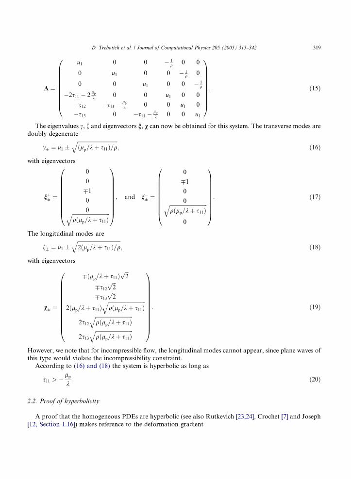
The eigenvalues c, f and eigenvectors n, v can now be obtained for this system. The transverse modes are

doubly degenerate

c� ¼ u1 �ffiffiffiffiffiffiffiffiffiffiffiffiffiffiffiffiffiffiffiffiffiffiffiffiffiffiffiffiffiffiðlp=kþ s11Þ=q

q; ð16Þ

with eigenvectors

nþ� ¼

0

0

�1

0

0ffiffiffiffiffiffiffiffiffiffiffiffiffiffiffiffiffiffiffiffiffiffiffiffiffiffiffiffiqðlp=kþ s11Þ

q

0BBBBBBBBB@

1CCCCCCCCCA; and n�� ¼

0

�1

0

0ffiffiffiffiffiffiffiffiffiffiffiffiffiffiffiffiffiffiffiffiffiffiffiffiffiffiffiffiqðlp=kþ s11Þ

q0

0BBBBBBBBB@

1CCCCCCCCCA: ð17Þ

The longitudinal modes are

f� ¼ u1 �ffiffiffiffiffiffiffiffiffiffiffiffiffiffiffiffiffiffiffiffiffiffiffiffiffiffiffiffiffiffiffiffi2ðlp=kþ s11Þ=q

q; ð18Þ

with eigenvectors

v� ¼

�ðlp=kþ s11Þffiffiffi2

p

�s12ffiffiffi2

p

�s13ffiffiffi2

p

2ðlp=kþ s11Þffiffiffiffiffiffiffiffiffiffiffiffiffiffiffiffiffiffiffiffiffiffiffiffiffiffiffiffiqðlp=kþ s11Þ

q

2s12ffiffiffiffiffiffiffiffiffiffiffiffiffiffiffiffiffiffiffiffiffiffiffiffiffiffiffiffiqðlp=kþ s11Þ

q

2s13ffiffiffiffiffiffiffiffiffiffiffiffiffiffiffiffiffiffiffiffiffiffiffiffiffiffiffiffiqðlp=kþ s11Þ

q

0BBBBBBBBBBBB@

1CCCCCCCCCCCCA

: ð19Þ

However, we note that for incompressible flow, the longitudinal modes cannot appear, since plane waves of

this type would violate the incompressibility constraint.

According to (16) and (18) the system is hyperbolic as long as

s11 > �lp

k: ð20Þ

2.2. Proof of hyperbolicity

A proof that the homogeneous PDEs are hyperbolic (see also Rutkevich [23,24], Crochet [7] and Joseph

[12, Section 1.16]) makes reference to the deformation gradient


F ¼ ox

oXð21Þ

relating a spatial (Eulerian) coordinate system {x} to a material (Lagrangian) coordinate system {X}. The

Jacobian J = det(F) is the ratio of material specific volume (1/q) to specific volume in the material reference

frame. Since J is strictly positive, the inverse of F exists:

g ¼ F�1 ð22Þ
is the inverse deformation gradient. The symmetric tensor ggT is positive definite.
The velocity gradient may be written in terms of the material derivative ðddtÞ of the deformation gradient:

ouaoxb

¼ dF ac

dtgcb: ð23Þ

Using this result, the upper-convected Maxwell derivative of any tensor H,

Hr� dH

dt� ðruÞH�HðruÞT ð24Þ

may be written

gHrgT ¼ d

dtgHgT� �

: ð25Þ

The stress equation (7) may therefore be written

d

dtðgsgTÞ þ 1

kgsgT ¼ �

lp

kd

dtðggTÞ; ð26Þ

with solution

g sþlp

kI

� gT ¼

lp

k2

Z t

�1ds eðs�tÞ=kggT: ð27Þ

Now, since ggT is positive definite, gðsþ lpk IÞgT is also positive definite, and so too is sþ lp

k I. The diagonal

elements of a positive definite tensor must be positive, so s11 þlpk > 0, and therefore the homogeneous

PDEs (11) and (12) are hyperbolic.

3. Design of new algorithm

Now that we have shown the hyperbolic nature of the stress equation (7) we can exploit this result to

design a new algorithm that makes use of the advantages of a BCG-type projection method while capturing

the viscous and elastic limits of the stress equation. We begin by using the previous linear analysis to cast

the stress equation (7) in a relatively simple form in terms of the inverse deformation gradient g:

d

dtðgsgTÞ ¼ � 1

kðgsgTÞ þ lp

d

dtðggTÞ

� �: ð28Þ

Integrating (28) from tn to tn+1 = tn + Dt, using Duhamel�s formula and the mean value theorem, we obtain

ðgsgTÞnþ1 ¼ ðgsgTÞne�Dtk �

Z Dt

0

e�ðDt�sÞ

klp

kd

dtðggTÞds ð29Þ

¼ ðgsgTÞne�Dtk þ 2lpðgDgTÞ 1� e�Dt=k

�; ð30Þ


with

d

dtðggTÞ ¼ 2gDgT; ð31Þ

where D ¼ 12½ðruÞ þ ðruÞT� and the overbar denotes a mean value in the range from 0 to Dt.

We then recognize the two important limits for our algorithm design. First as the relaxation time

approaches zero, k ! 0, the polymer stress equilibrates instantly with the polymer viscous stress:

s ¼ lpðruþruTÞðk ! 0Þ: ð32Þ

In this equilibrium limit, (30) becomes

ðgsgTÞnþ1 ¼ 2lpgDgTðk ! 0Þ: ð33Þ

Second, as the relaxation time increases without bound, the polymer stress equation becomes

os

otþ u � rs� ðruÞs� sðruÞT ¼

lp

kðruþruTÞðk ! 1Þ: ð34Þ

(Here we require that lp/k approaches a definite nonzero limit.) In this fully decoupled limit the integral

expression (30) becomes

ðgsgTÞnþ1 ¼ ðgsgTÞn �lp

kðggTÞnþ1 � ðggTÞnh i

ðk ! 1Þ: ð35Þ

In order to assure recovery of these limits in a discretization of (28), we introduce a factor C(k) with the

following properties:

limk!0

CðkÞ ¼ OðkÞ; ð36Þ

limk!1

CðkÞ ¼ 1: ð37Þ

For example,

CðkÞ ¼ 1� e�Kk=tadv ; ð38Þ
where K is a positive constant, e.g., K = 1 or K = r, and r < 1 is the CFL number. Also, we note use of
the parameter, tadv, instead of Dt. This advective time scale on a discrete grid is obtained by applying

the advective limit, and, thus, it is defined as the ratio of discrete grid spacing to the maximum fluid

velocity,

tadv ¼ Dx=maxi;j;k

juj; ð39Þ

where Dx corresponds to the grid spacing in the direction of maximum u, at the maximum velocity�s discretecell center (i, j,k). By choosing tadv to be independent of Dt, a stable Dt can be constructed explicitly from

the CFL condition in our discretization. We will also show that this choice of time scale obeys the design

limits of the algorithm (48) and (47).

We may use C(k) to isolate the limiting parts of (30), and rearrange to give

ðgsgTÞnþ1 � ðgsgTÞn

Dt¼ �ðgsgTÞn

1� e�Dt=k �

Dtþ 2lpðgDgTÞ

1� e�Dt=k �

Dt½1� CðkÞ� þ 2

�lp

kðgDgTÞCðkÞk

1� e�Dt=k �

Dt: ð40Þ


This discretization of (30) recovers the desired limits. As k ! 0,


Dt¼ �ðgsgTÞn 1

Dtþ 2lpðgDgTÞ 1

Dt; ð41Þ

and as k ! 1 (with k(1 � e�Dt/k) ! Dt)


Dt¼ 2

lp

kðgDgTÞ ¼

k!1�lp

kðggTÞnþ1 � ðggTÞn

Dt: ð42Þ

Let us associate the part surviving k ! 1 with an explicit hyperbolic scheme having the form

o

otðgsgTÞ � 2a2ðgDgTÞ ¼ � � � ð43Þ

This choice is motivated by the fact that in the fully uncoupled limit (34) may be written as a conservation

law accurately modeled with higher-order advection schemes:

d

dtgðsþ

lp

kIÞgT ¼ 0: ð44Þ

By comparing (43) with (40) we define a wavespeed

a2 ¼ aðkÞa21 þ ½1� aðkÞ�a20; ð45Þ

aðkÞ ¼ kDt

CðkÞ 1� e�Dt=k �

; ð46Þ

a21 ¼ limk!1

a2 ¼lp

k; ð47Þ

while retaining some elastic freedom in recovering the viscous limit

a20 ¼ limk!0

a2 ¼ gs: ð48Þ

We define s as the absolute value of the global minimum of the normal stresses, s = jminb(sbb)j, and g is a

positive control parameter usually equal to 1.

Also, the remainder, or right-hand side, from comparing (43) with (40) contains a proper source term

and gradient viscous terms

� 1

kðgsgTÞ � 2lpðgDgTÞ �

� 2a2ðgDgTÞ: ð49Þ

All together, the stress equation (7) becomes

os

otþ u � rs� ðruÞs� sðruÞT � a2 ðruÞ þ ðruTÞ

�¼ � 1

ksþ

lp

k� a2

h iðruÞ þ ðruÞTh i

: ð50Þ

From here, our approach is to discretize (50) using an unsplit Lax–Wendroff method which is appropri-ate for the hyperbolic left-hand side; and an implicit discretization of the right-hand side to recover the

viscous limit as k ! 0.

4. Discretization method

We discretize the equations of motion (5), (6) and (50) using a high-resolution finite difference method to

evolve velocity, pressure and stress in time. Time is represented in discrete time steps as t = (n + 1)Dt,n = 0, 1, 2, . . . At the beginning of each time step we know cell-centered Cartesian grid representations

of velocity, pressure and stress: uni;j;k, rpni;j;k; sni;j;k.


4.1. Velocity discretization

We summarize the velocity discretization following ideas in [4]. The projection operator is used to ad-

vance the velocity in time while enforcing incompressibility

unþ1 ¼ u� þ Dtqrpn�

12 � ðI�PÞ u� þ Dt

qrpn�

12

� �; ð51Þ

rpnþ12 ¼ q

DtðI�PÞ u� þ Dt

qrpn�

12

� �; ð52Þ

where Q ¼ GL�1D, P ¼ I� Q, L ¼ DG and D and G are numerical divergence and gradient operators,respectively, and pressure formulation is employed.

To predict the intermediate velocity, u*, we first construct edge-centered velocities using a Lax–Wendroff

(LW) discretization of the PDE, omitting the pressure gradient (for now)

~uiþ12;j;k ¼

1

2ðuni;j;k þ uniþ1;j;kÞ þ

Dt2

�ðu � rÞuþ ls

qDuþ 1

qr � s

� �n

iþ12;j;k

: ð53Þ

A projection is then applied to the edge-centered velocities to correct for the omitted pressure term in the

previous step

unþ1

2

iþ12;j;k

¼ ~uiþ12;j;k �rðD�1ðr � ~uÞÞiþ1

2;j;k: ð54Þ

In this predictor step we use inviscid, no-flow boundary conditions, or u � n̂ ¼ 0 at solid walls, ouon̂¼ 0 at out-

flow, prescribed velocity at inflow and extrapolation on transverse components.

We obtain u* using the midpoint rule for temporal integration

u� ¼ un þ Dt �½ðu � rÞu�nþ12 � 1

qrpn�

12 þ ls

qDu� þ 1

qðr � sÞnþ

12

� �; ð55Þ

where the viscous stresses are calculated using the backward Euler method, the half time advective term is

calculated using the edge velocities in (54) and snþ12 is defined below in (62). We note that u* is not diver-

gence-free by O(Dt2) because of a lagged pressure gradient.

The equation used to predict the solution to the viscous problem has the following form:

Lmu� ¼ un þ Dt �ðu � rÞunþ1

2 � 1

qrpn�

12 þ 1

q2k

2kþ Dtðr � ~sÞ

� �; ð56Þ

where

Lm ¼ I� Dtq

ls þðlp � ka2ÞDt

2kþ Dt

� �D; ð57Þ

and ~s is defined below in (60). The boundary conditions for the viscous problem are u � n̂ ¼ 0 at solid walls,ouon̂¼ 0 at outflow and prescribed velocity at inflow, which is implemented using residual correction.

A final projection operator is applied to the predicted velocity, u*, in pressure formulation, enforcing the

incompressibility constraint on the velocity and updating the pressure gradient:

unþ1 ¼ u� þ Dtqrpn�

12 �r D�1 r � u� þ Dt

qrpn�

12

� �� ; ð58Þ


rpnþ12 ¼ q

Dtr D�1 r � u� þ Dt

qrpn�

12

� �� : ð59Þ

Projection boundary conditions are u � n̂ ¼ 0, opon̂¼ 0 at solid walls, ou

on̂¼ 0, p = 0 at outflow and prescribed

velocity with opon̂¼ 0 at inflow. Also, the final projection yields a divergence-free velocity field which may

contain unphysical checkerboard modes due to centered differencing. We use a simple, single-step filter

to eliminate these modes [16,22,9].

4.2. Stress discretization

The stress discretization follows a similar algorithm as in [25]. First, we construct a Lax–Wendroff stress

using only the elastic (hyperbolic) terms:

~siþ12;j;k ¼

1

2ðsni;j;k þ sniþ1;j;kÞ þ

Dt2

�ðu � rÞsþru � ðsþ a2IÞ þ ðsþ a2IÞ � ruT� �n

iþ12;j;k: ð60Þ

We then predict a half time stress for the viscous problem, again, using the backward Euler method for

viscous stresses

snþ1

2

iþ12;j;k

¼ ~siþ12;j;k �

Dt2

1

ksnþ1

2

iþ12;j;k

� 2lp

k� a2

� Dðu�Þ

� �ð61Þ

¼ 2

2kþ Dtk~siþ1

2;j;k þ Dtðlp � ka2ÞDðu�Þ

� : ð62Þ

The stress is updated to the new time as follows:

snþ1 ¼ sn þ Dt �ðu � rÞsþru � sþ a2IÞ þ ðsþ a2IÞ � ruT� �nþ1

2 � Dtkðsnþ1 � 2ðlp � a2kÞDðunþ1ÞÞ ð63Þ

¼ kkþ Dt

sn þ Dt �½ðu � rÞs� þ ðru � ðsþ a2IÞÞ þ ððsþ a2IÞ � ruTÞ� nþ1

2 þ 2lp

k� a2

� Dðunþ1Þ

h i� :

ð64Þ

Stress boundary conditions are implemented numerically using a zeroth-order extrapolation. For the nor-mal components of the stress this condition is justified by the characteristic analysis in Section 2.1 plus the

assumption that a uniform elastic stress distribution will, by itself, generate no waves. The tangential com-

ponents on boundary edges are not used. At inflow, if Poiseuille flow is specified, then we use self-consistent

stress boundary conditions; if plug inflow, then homogeneous Dirichlet stress conditions.

4.3. Stability

We have applied von Neumann stability analysis to the Lax–Wendroff method in general. In 2D we con-sider the scalar advection equation

ouot

þ aouox

þ bouoy

¼ 0 ð65Þ

on a periodic domain with given initial conditions [10]. A sufficient condition for the method to be stable in

the long wavelength limit is

r2xn

4x þ r2

yn4x > ðrxnx þ rynxÞ4; ð66Þ

where rx ¼ aDtDx , ry ¼ bDt

Dy and (nx,ny) are components of the unit normal for the orthonormal basis formed by

the complex exponentials on the given interval. This sufficiency condition yields a CFL number of

jrxj; jry j < 14. In 3D, we obtain a slightly more restrictive CFL of jrxj; jry j; jrzj < 1

9.


For our method a stable time step is obtained from the following advective CFL condition ðr < 19Þ:

maxi;j;k

½jui;j;kj þ ð2ðsxx þ a2Þ=qÞ12�Dt < rDx; ð67Þ

maxi;j;k

½jvi;j;kj þ ð2ðsyy þ a2Þ=qÞ12�Dt < rDy; ð68Þ

maxi;j;k

½jwi;j;kj þ ð2ðszz þ a2Þ=qÞ12�Dt < rDz: ð69Þ

4.4. Viscoelastic limits of algorithm

The viscous limit of our method, k ¼ 0 ) a2 ¼ 0, reveals the stress of a Newtonian fluid with augmented

viscosity due to the polymer:

snþ1

2

iþ12;j;k

¼ 2lpDðu�Þ; ð70Þ

snþ1 ¼ 2lpDðunþ1Þ; ð71Þ

Lm ¼ I�ðls þ lpÞDt

qD: ð72Þ

The elastic limit of the method, k ! 1; lp=k finite ) a2 ! lp=k, demonstrates the hyperbolic nature,

with finite, non-zero wavespeed, which the stress discretization assumes in this limit, with no viscous con-

tribution by the polymer:

snþ1

2

iþ12;j;k

¼ ~siþ12;j;k ð73Þ

¼ 1

2ðsni;j;k þ sniþ1;j;kÞ þ

Dt2

�ðu � rÞsþru � sþlp

kI

� þ sþ

lp

kI

� � ruT

� n

iþ12;j;k; ð74Þ

snþ1 ¼ sn þ Dt �ðu � rÞsþru � sþlp

kI

� þ sþ

lp

kI

� � ruT

� nþ12

; ð75Þ

Lm ¼ I� lsDtq

D: ð76Þ

For Maxwell fluids where ls = 0 we note that no-slip boundary conditions are not imposed because the vis-

cous terms vanish.

5. Results

We apply the method to unsteady flow of Oldroyd-B fluids in abrupt planar contraction channels (Fig.

1). First, we simulate the Oldroyd-B fluid without viscosity (ls = 0) in sudden contraction channels to

demonstrate stable and convergent calculation of the flow of an unsteady Maxwell fluid, which allows

finite elastic wave propagation. We then add some viscosity to the Maxwell fluid and demonstrate stable


and convergent simulations at high We in abrupt contractions for unsteady flow with hybrid viscous and

elastic behavior. Next we present results for the viscous limit of an Oldroyd-B fluid in abrupt contraction

channels. Finally, we show stable and convergent results for benchmark high Weissenberg number prob-

lems at We = 1 and We = 10. We characterize our results with the elastic Mach number and Weissenberg

number where the characteristic velocity, U, is the average velocity in the contraction channel, or theaverage inflow velocity times the contraction ratio. We demonstrate accuracy of the method for each

case. For viscous flows convergence results are obtained away from the inlet of the channel in order

to isolate the re-entrant corner and to omit known singularities at the inlet due to prescribed constant

velocity boundary conditions. The method is valid for both 2D and 3D flows, though only 2D results

are shown here for simplicity in demonstrating the robustness of the algorithm. For 3D results we refer

to our previous work in [25].

5.1. Flow of a Maxwell fluid

The example which best demonstrates the robustness of our method is the unsteady flow of a Maxwell

fluid. Again, the Maxwell fluid is the Oldroyd-B fluid with ls = 0; also, propagation of waves with finite

elastic wave speeds is allowed. We show results for flow of a Maxwell fluid in both 2:1 and 4:1 contractions.

Figs. 2 and 3 are time sequences of velocity that demonstrate convergence forWe = 205.6,Ma = .31 in a 2:1

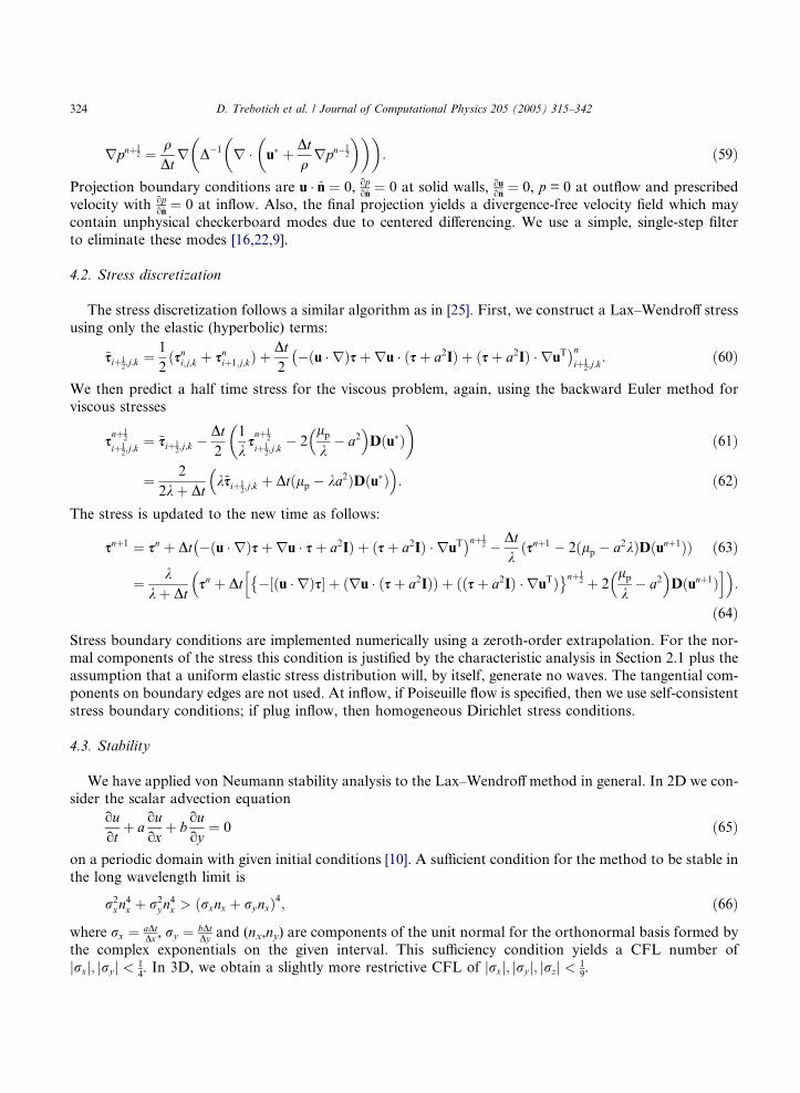
contraction and We = 822.4, Ma = .62 in a 4:1 contraction, respectively. Figs. 4 and 5 show the difference

between pressures for the viscous limit and elastic flow, clearly demonstrating the wave behavior in the

Maxwell fluid. In Tables 1 and 2 we show convergence results for the Maxwell fluid at very long time:Ma = 0.3, We = 205.6 in 2:1 contraction; Ma = 0.6, We = 822.4 in 4:1 contraction. The solution shows sec-

ond-order convergence in L1 and L2 norms and only first-order convergence in L1 norm. We attribute the

slight drop off in convergence in the L1 norm to the geometric singularity and wave interactions. We note

again that the no-slip boundary condition is not imposed because of the vanishing viscous terms in these

flows.

We make several observations from the flow data in the Maxwell fluid case. First, we note that elastic

wave behavior is captured in these results using the same algorithm and same stability condition as the re-

sults generated for the more viscous fluids seen in later sections. Second, these results are valid for very longtime without violating hyperbolicity and while maintaining stability and convergence, even though there is

a build up of stress at corners. Third, results for the Maxwell fluid are not limited byWe, but only subject to

subcritical elastic Mach number with lp/k finite for well-posedness in the elastic limit, or lp/k > qU2. Final-

ly, we have not physically validated the computed behavior, though the solution does clearly converge and

is not a numerical artifact.

5.2. Hybrid flow of a Maxwell fluid with viscosity

We have also applied the method to flows of Maxwell fluids with viscosity in planar contractions to

demonstrate mixed viscous and elastic effects. For regimes where the solvent viscosity is large enough

we do not note much difference in the solution from viscous limit examples. However, for hybrid flows,

where the elastic waves interact with viscous forces we find that there is definite unsteady behavior.

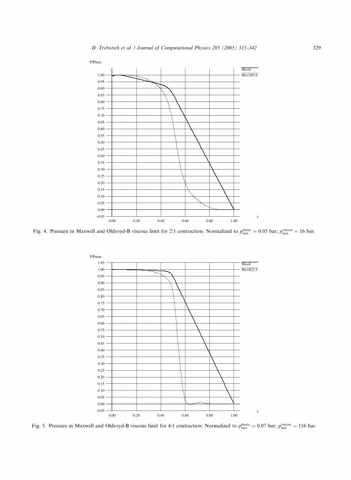
Time sequences of velocity in 2:1 (Ma = 0.06, We = 8) and 4:1 contractions (Ma = 0.12, We = 32) are

shown in Figs. 6 and 7, respectively, demonstrating that the flow is viscous, though not a classic par-

abolic velocity profile due to the effect of elastic shear waves. More experimentation is needed to quan-

tify the extent of this behavior and to determine the critical values of We at which the transition tohybrid, unsteady behavior occurs [17]. In Tables 3 and 4 we show convergence rates at early times.

Fig. 2. Convergence of Maxwell fluid in 2:1 contraction, Ma = 0.3, We = 205.6. (L) 200 time step increments, h = 1/128; (R) 400 time

step increments, h = 1/256.


Fig. 3. Convergence of Maxwell fluid in 4:1 contraction, Ma = 0.6, We = 822.4. (L) 200 time step increments, h = 1/128; (R) 400 time

step increments, h = 1/256.


We=0

We=205.6

P/Pmax

z-0.05

0.00

0.05

0.10

0.15

0.20

0.25

0.30

0.35

0.40

0.45

0.50

0.55

0.60

0.65

0.70

0.75

0.80

0.85

0.90

0.95

1.00

0.00 0.20 0.40 0.60 0.80 1.00

Fig. 4. Pressure in Maxwell and Oldroyd-B viscous limit for 2:1 contraction. Normalized to pelasticmax ¼ 0:03 bar; pviscousmax ¼ 16 bar.

We=0

We=822.4

P/Pmax

z-0.05

0.00

0.05

0.10

0.15

0.20

0.25

0.30

0.35

0.40

0.45

0.50

0.55

0.60

0.65

0.70

0.75

0.80

0.85

0.90

0.95

1.00

1.05

0.00 0.20 0.40 0.60 0.80 1.00

Fig. 5. Pressure in Maxwell and Oldroyd-B viscous limit for 4:1 contraction. Normalized to pelasticmax ¼ 0:07 bar; pviscousmax ¼ 116 bar.



In Tables 5–7 we show convergence rates at late times. The solution does not show second-order con-

vergence, as expected, due to the use of backward Euler for viscous stresses, but it is better than first-

order because the flow is not purely viscous. We attribute the drop off in convergence in the L1 norm

to the presence of the viscous effects interacting with elastic waves near the corner singularity. We also

note the drop off in the L1 norm at the late times, seen in Table 7 and the last frames of Fig. 7 for the4:1 contraction.

5.3. Viscous limit of Oldroyd-B

We demonstrate convergence of velocity in the viscous limit (We = 0) of an Oldroyd-B fluid for both

2:1 and 4:1 contractions in Fig. 8. We note singularities at both inflow (due to constant velocity bound-

ary condition) and re-entrant corners. We show convergence rates for this data in Tables 8 and 9. The

convergence rates are first-order, as expected, due to the use of backward Euler for viscous stresses. Inthe L1 norm the results are Oðh1

2Þ due to the presence of geometric singularities at re-entrant corners. We

also note the restriction on the time step in the viscous limit. The maximum advective velocity for these

flows is approximately 0.05 while the wavespeed which uses a2 is about 1.5, demonstrating the slight

restriction on time step in our method, about a factor of 30. However, by comparison, if the elastic wave-

speed is used to determine the time step in this viscous case as in [15], then the restriction is much greater,

or a factor of 106.

5.4. Benchmark viscoelastic flow

We present stable and convergent results for the benchmark problem of steady viscoelastic flow of an

Oldroyd-B fluid in a 4:1 contraction for We = 1, Re = 1 and Re = 0 and b ” ls/l = 1/9. We emulate the

problem parameters – steady state solution criterion, maximum time step for steady-state convergence,

Table 1

Error and convergence rates for transverse (left) and axial (right) velocity of Maxwell fluid, Ma = 0.3, We = 205.6 in 2:1 contraction

channel at 2328 time steps (h = 1/256)

Norm u w

e1/64 Rate e1/128 e1/64 Rate e1/128

L1 5.24 · 10�3 1.78 1.54 · 10�3 6.66 · 10�1 2.16 1.49 · 10�1

L2 5.28 · 10�3 1.42 1.98 · 10�3 4.90 · 10�1 1.47 1.77 · 10�1

L1 1.47 · 10�2 0.52 1.03 · 10�2 9.65 · 10�1 0.52 6.75 · 10�1

Table 2

Error and convergence rates for transverse (left) and axial (right) velocity of Maxwell fluid, Ma = 0.6, We = 822.4 in 4:1 contraction


Norm u w

e1/64 Rate e1/128 e1/64 Rate e1/128

L1 6.44 · 10�3 2.06 1.54 · 10�3 5.69 · 10�1 2.40 1.08 · 10�1

L2 7.19 · 10�3 1.56 2.44 · 10�3 5.36 · 10�1 1.75 1.59 · 10�1

L1 2.72 · 10�2 0.97 1.39 · 10�2 1.65 0.84 9.19 · 10�1

Fig. 6. Convergence of Maxwell fluid with viscosity in 2:1 contraction,Ma = 0.06,We = 8. (L) 200 time step increments, h = 1/128; (R)

400 time step increments, h = 1/256.


Fig. 7. Convergence of Maxwell fluid with viscosity in 4:1 contraction, Ma = 0.13, We = 32. (L) 200 time step increments, h = 1/128;

(R) 400 time step increments, h = 1/256.


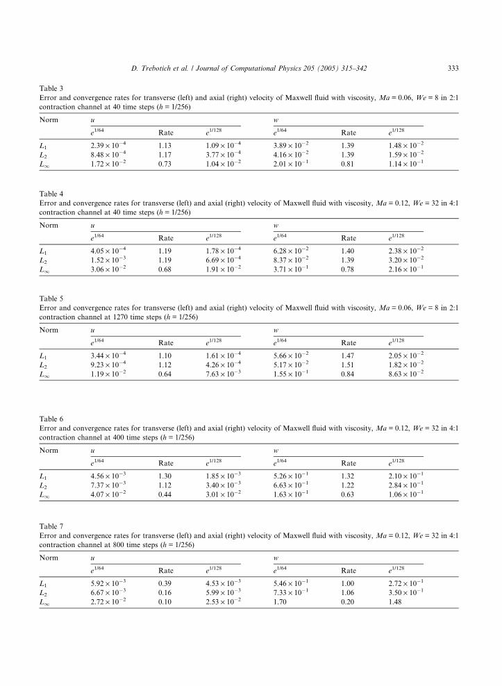
Table 3

Error and convergence rates for transverse (left) and axial (right) velocity of Maxwell fluid with viscosity, Ma = 0.06, We = 8 in 2:1

contraction channel at 40 time steps (h = 1/256)

Norm u w

e1/64 Rate e1/128 e1/64 Rate e1/128

L1 2.39 · 10�4 1.13 1.09 · 10�4 3.89 · 10�2 1.39 1.48 · 10�2

L2 8.48 · 10�4 1.17 3.77 · 10�4 4.16 · 10�2 1.39 1.59 · 10�2

L1 1.72 · 10�2 0.73 1.04 · 10�2 2.01 · 10�1 0.81 1.14 · 10�1

Table 4



Norm u w

e1/64 Rate e1/128 e1/64 Rate e1/128

L1 4.05 · 10�4 1.19 1.78 · 10�4 6.28 · 10�2 1.40 2.38 · 10�2

L2 1.52 · 10�3 1.19 6.69 · 10�4 8.37 · 10�2 1.39 3.20 · 10�2

L1 3.06 · 10�2 0.68 1.91 · 10�2 3.71 · 10�1 0.78 2.16 · 10�1

Table 7



Norm u w

e1/64 Rate e1/128 e1/64 Rate e1/128

L1 5.92 · 10�3 0.39 4.53 · 10�3 5.46 · 10�1 1.00 2.72 · 10�1

L2 6.67 · 10�3 0.16 5.99 · 10�3 7.33 · 10�1 1.06 3.50 · 10�1

L1 2.72 · 10�2 0.10 2.53 · 10�2 1.70 0.20 1.48

Table 6



Norm u w

e1/64 Rate e1/128 e1/64 Rate e1/128

L1 4.56 · 10�3 1.30 1.85 · 10�3 5.26 · 10�1 1.32 2.10 · 10�1

L2 7.37 · 10�3 1.12 3.40 · 10�3 6.63 · 10�1 1.22 2.84 · 10�1

L1 4.07 · 10�2 0.44 3.01 · 10�2 1.63 · 10�1 0.63 1.06 · 10�1

Table 5



Norm u w

e1/64 Rate e1/128 e1/64 Rate e1/128

L1 3.44 · 10�4 1.10 1.61 · 10�4 5.66 · 10�2 1.47 2.05 · 10�2

L2 9.23 · 10�4 1.12 4.26 · 10�4 5.17 · 10�2 1.51 1.82 · 10�2

L1 1.19 · 10�2 0.64 7.63 · 10�3 1.55 · 10�1 0.84 8.63 · 10�2


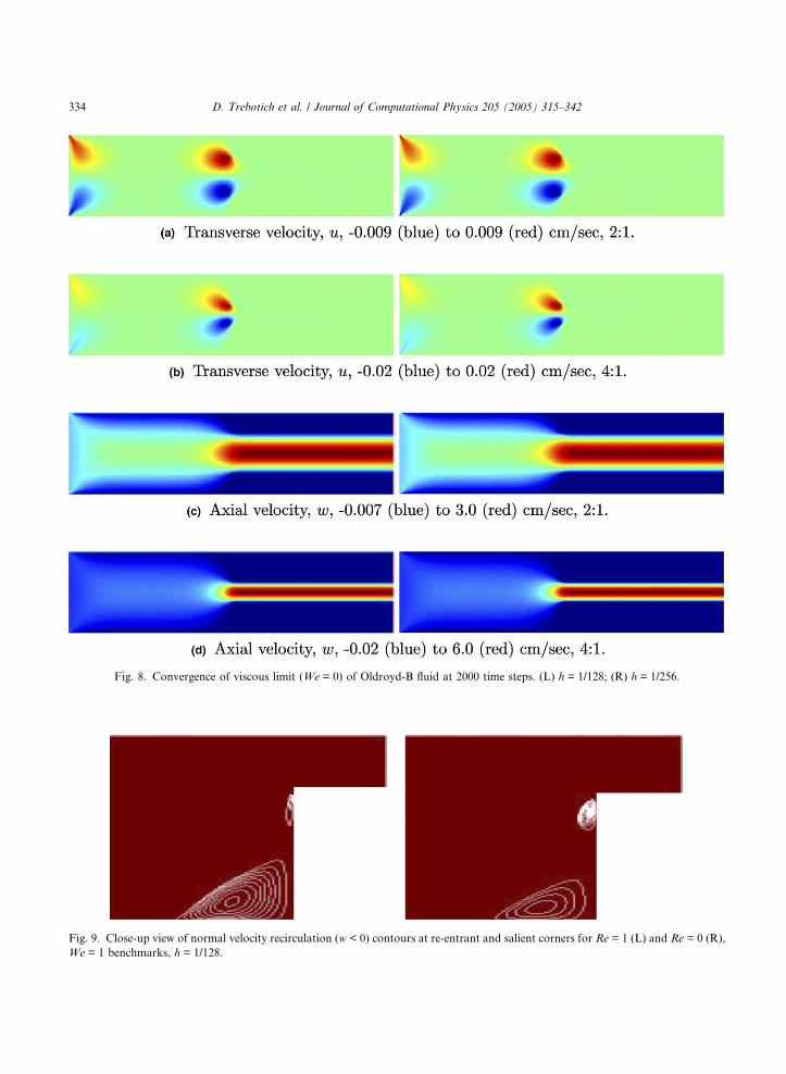
Fig. 8. Convergence of viscous limit (We = 0) of Oldroyd-B fluid at 2000 time steps. (L) h = 1/128; (R) h = 1/256.

Fig. 9. Close-up view of normal velocity recirculation (w < 0) contours at re-entrant and salient corners for Re = 1 (L) and Re = 0 (R),

We = 1 benchmarks, h = 1/128.


Table 9

Error and convergence rates for transverse (left) and axial (right) velocity of viscous limit (We = 0) Oldroyd-B fluid in 4:1 contraction


Norm u w

e1/64 Rate e1/128 e1/64 Rate e1/128

L1 6.36 · 10�5 0.96 3.27 · 10�5 1.06 · 10�2 1.31 4.29 · 10�3

L2 1.89 · 10�4 0.82 1.07 · 10�4 2.15 · 10�2 1.02 1.06 · 10�2

L1 3.32 · 10�3 0.45 2.44 · 10�3 3.08 · 10�1 0.50 2.18 · 10�1

Table 10

Error and convergence rates for transverse (left) and normal (right) velocity for benchmark problem We = 1, Re = 1, Ma = 0.75 in 4:1

contraction channel at steady-state (1290 time steps, h = 1/512, r = 0.25 or Dtmin = 9 · 10�5)

Norm u w

e1/128 Rate e1/256 e1/128 Rate e1/256

L1 7.60 · 10�3 1.22 3.27 · 10�3 6.99 · 10�2 1.53 2.42 · 10�2

L2 1.38 · 10�2 0.81 7.88 · 10�3 7.71 · 10�2 1.44 2.84 · 10�2

L1 1.11 · 10�1 0.29 9.10 · 10�2 4.29 · 10�1 0.39 3.27 · 10�1

Table 11

Error and convergence rates for transverse (left) and normal (right) velocity for benchmark problem We = 1, Re = 0, Ma1 in 4:1

contraction channel at steady-state (244 time steps, h = 1/128, Dt = 8 · 10�5)

Norm u w

e1/32 Rate e1/64 e1/32 Rate e1/64

L1 2.12 · 10�6 1.37 8.18 · 10�7 4.14 · 10�6 1.57 1.39 · 10�6

L2 3.71 · 10�6 1.05 1.79 · 10�6 6.26 · 10�6 1.24 2.65 · 10�6

L1 1.91 · 10�5 0.75 1.13 · 10�5 3.07 · 10�5 0.74 1.84 · 10�5

Table 8

Error and convergence rates for transverse (left) and axial (right) velocity of viscous limit (We = 0) Oldroyd-B fluid in 2:1 contraction


Norm u w

e1/64 Rate e1/128 e1/64 Rate e1/128

L1 5.43 · 10�5 1.04 2.64 · 10�5 6.40 · 10�3 1.18 2.83 · 10�3

L2 1.03 · 10�4 0.90 5.51 · 10�5 9.96 · 10�3 0.99 5.00 · 10�3

L1 1.32 · 10�3 1.23 5.62 · 10�4 1.17 · 10�1 1.28 4.83 · 10�2


h=1/512

h=1/256

h=1/128

h=1/64

tau_zz

-3z x 10

0.00

20.00

40.00

60.00

80.00

100.00

120.00

140.00

160.00

180.00

200.00

220.00

240.00

260.00

460.00 480.00 500.00 520.00 540.00

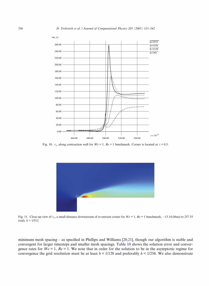
Fig. 10. szz along contraction wall for We = 1, Re = 1 benchmark. Corner is located at z = 0.5.

Fig. 11. Close-up view of szz a small distance downstream of re-entrant corner for We = 1, Re = 1 benchmark, �13.14 (blue) to 257.55

(red), h = 1/512.


minimum mesh spacing – as specified in Phillips and Williams [20,21], though our algorithm is stable and

convergent for larger timesteps and smaller mesh spacings. Table 10 shows the solution error and conver-

gence rates for We = 1, Re = 1. We note that in order for the solution to be in the asymptotic regime for

convergence the grid resolution must be at least h < 1/128 and preferably h < 1/256. We also demonstrate

1/512

1/256

1/128

1/64

tau_xz

-3z x 10-130.00

-120.00

-110.00

-100.00

-90.00

-80.00

-70.00

-60.00

-50.00

-40.00

-30.00

-20.00

-10.00

0.00

460.00 480.00 500.00 520.00 540.00

Fig. 12. sxz along contraction wall for We = 1, Re = 1 benchmark. Corner is located at z = 0.5.

h=1/256

h=1/128

h=1/64

error x 10-3

-3x x 10-450.00

-400.00

-350.00

-300.00

-250.00

-200.00

-150.00

-100.00

-50.00

-0.00

50.00

100.00

150.00

200.00

400.00 450.00 500.00 550.00 600.00

Fig. 13. Cross-section of error in normal velocity at maximum error location in z, a short distance downstream of re-entrant corner for

We = 1, Re = 1 benchmark. Centerline of channel is located at x = 0.5.


h=1/256

h=1/128

h=1/64

error x 10-3

-3x x 10

-160.00

-140.00

-120.00

-100.00

-80.00

-60.00

-40.00

-20.00

0.00

20.00

40.00

60.00

80.00

100.00

400.00 450.00 500.00 550.00 600.00

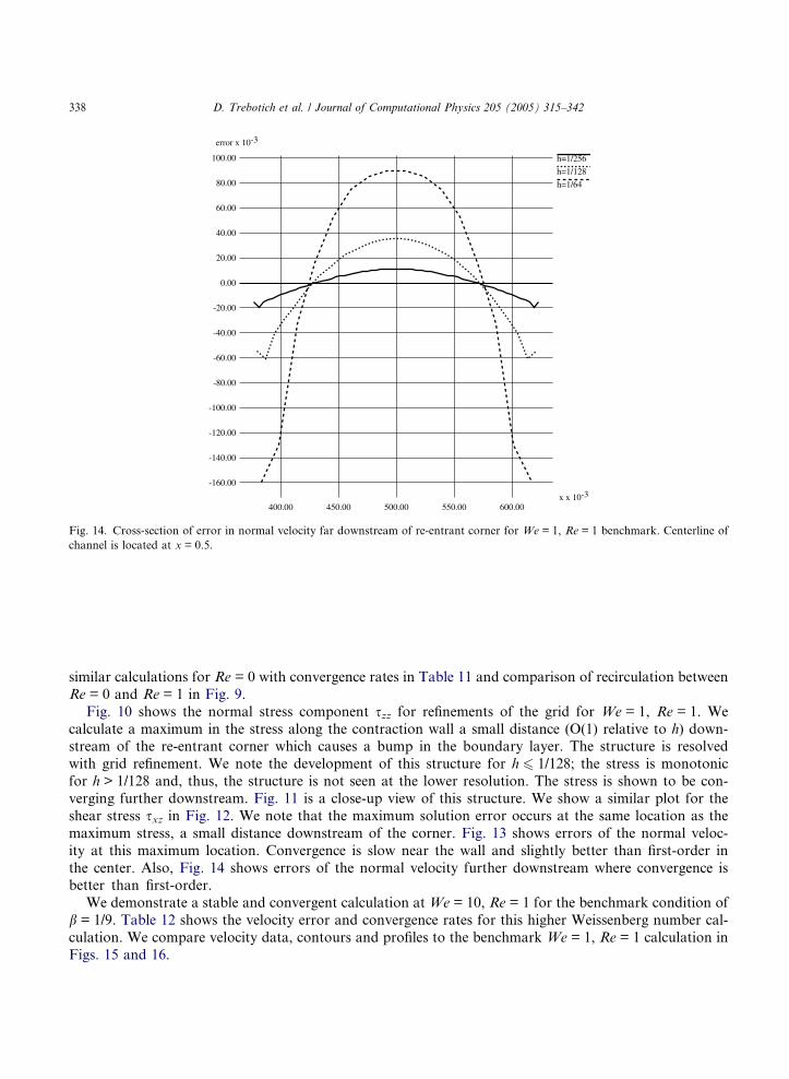
Fig. 14. Cross-section of error in normal velocity far downstream of re-entrant corner for We = 1, Re = 1 benchmark. Centerline of

channel is located at x = 0.5.


similar calculations for Re = 0 with convergence rates in Table 11 and comparison of recirculation between

Re = 0 and Re = 1 in Fig. 9.

Fig. 10 shows the normal stress component szz for refinements of the grid for We = 1, Re = 1. We

calculate a maximum in the stress along the contraction wall a small distance (O(1) relative to h) down-stream of the re-entrant corner which causes a bump in the boundary layer. The structure is resolved

with grid refinement. We note the development of this structure for h 6 1/128; the stress is monotonic

for h > 1/128 and, thus, the structure is not seen at the lower resolution. The stress is shown to be con-

verging further downstream. Fig. 11 is a close-up view of this structure. We show a similar plot for the

shear stress sxz in Fig. 12. We note that the maximum solution error occurs at the same location as the

maximum stress, a small distance downstream of the corner. Fig. 13 shows errors of the normal veloc-

ity at this maximum location. Convergence is slow near the wall and slightly better than first-order in

the center. Also, Fig. 14 shows errors of the normal velocity further downstream where convergence isbetter than first-order.

We demonstrate a stable and convergent calculation at We = 10, Re = 1 for the benchmark condition of

b = 1/9. Table 12 shows the velocity error and convergence rates for this higher Weissenberg number cal-

culation. We compare velocity data, contours and profiles to the benchmark We = 1, Re = 1 calculation in

Figs. 15 and 16.

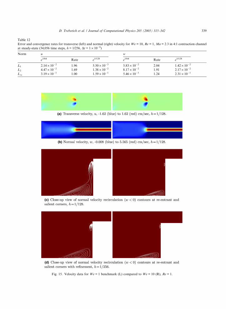
Fig. 15. Velocity data for We = 1 benchmark (L) compared to We = 10 (R), Re = 1.

Table 12

Error and convergence rates for transverse (left) and normal (right) velocity for We = 10, Re = 1, Ma = 2.3 in 4:1 contraction channel

at steady-state (34,056 time steps, h = 1/256, Dt = 1 · 10�6)

Norm u w

e1/64 Rate e1/128 e1/64 Rate e1/128

L1 2.14 · 10�2 1.96 5.50 · 10�3 5.83 · 10�2 2.04 1.42 · 10�2

L2 4.47 · 10�2 1.69 1.38 · 10�2 8.17 · 10�2 1.91 2.17 · 10�2

L1 3.19 · 10�1 1.00 1.59 · 10�1 5.46 · 10�1 1.24 2.31 · 10�1


We=10, z=.25

We=10, z=.75

We=10, z=.5

We=1, z=.25

We=1, z=.75

We=1, z=.5

w

x

0.00

0.50

1.00

1.50

2.00

2.50

3.00

3.50

4.00

4.50

5.00

5.50

0.00 0.20 0.40 0.60 0.80 1.00

Fig. 16. Normal velocity cross-sectional profiles for We = 1 benchmark (L) compared to We = 10 (R), Re = 1, h = 1/128.


6. Conclusions

We demonstrate a stable and convergent numerical method for viscoelastic flow in abrupt contraction

channels. The method is different from prior steady-state or implicit methods in that it is an appropriately

designed unsteady flow method which can capture wave motion in strongly elastic flows for any value of the

Weissenberg number and is only restricted by subcritical elastic Mach number. The method requires a sin-

gle CFL condition for the range of elastic flows, from the viscous limit to the elastic limit. This is achievedthrough a variation of the BCG projection method which obeys the desired viscous and elastic limits of the

equations of motion. In steady-state problems where the elastic Mach number is supercritical hyperbolicity

is maintained by imposing a slightly smaller timestep than that computed by the stability condition. For

Maxwell fluids we demonstrate unsteady results for arbitrarily high We and Ma < 1 where elastic shear

waves propagate in an incompressible fluid and are captured by the method in a stable and convergent

manner. The method has also been shown to be stable and convergent for unsteady high Weissenberg num-

ber flows of Maxwell fluids with viscosity in abrupt contractions. More experimentation is needed to quan-

tify the extent of the behavior (vortex enhancement, for example) in these flows. The method also calculatesthe viscous limit of the Oldroyd-B equation, with a time step restricted only slightly more than that gov-

erned by the advective velocity alone. The method compares very well to known exact solutions and pre-

liminary data from experimental flows in microfluidic devices [25].

Finally, we show a stable and convergent calculation of high Weissenberg number flows for We = 1 and

We = 10. We demonstrate our method for the benchmark problem and show that the algorithm is capable

of resolving non-singular structure in the stress along the contraction wall a short distance (O(1) relative to

h) downstream of the re-entrant corner. We note that in the many previous works on the benchmark prob-

lem, summarized in [20,21,3], the methods employed break down around We = 2 – that is, they fail to


achieve steady-state, and they do not converge numerically. This observed critical Weissenberg number

with Re = 1 corresponds to the critical elastic Mach number,Ma = 1, where waves are no longer suppressed

at supercritical values. We notice this wave behavior gradually with increasing We. For supercritical flows

steady-state solutions are not necessarily attainable, but stable and numerically convergent results are. We

are able to capture this behavior, as demonstrated above with the results for Maxwell flows with and with-out viscosity, and also with higher Weissenberg number flows in the benchmark parameter regime. Our cal-

culation of a higher Weissenberg number, We = 10, Ma = 2.3, is a first for this regime of flows. We do not

observe a limiting value of We in benchmark problems.

In the future we will modify the scheme in several ways. To improve the accuracy of viscous flows to

second-order, we will implement the implicit Runge–Kutta scheme of Twizell, Gumel and Arigu in [26]

for the viscous stresses as it is known to be L0-stable in the presence of boundaries, unlike Crank–Nicolson

[11]. We will also take advantage of the ability to cast the PDEs (5) and (7) in a hybrid conservation form

which exploits hyperbolicity while maintaining the viscous and elastic limits. This means we will naturallyextend the method to make use of the higher-order Godunov method of the BCG formulation, allowing us

to eliminate any subcritical Mach number restriction. Higher-order Godunov methods are more robust

than LW for hyperbolic systems; and the CFL time step is an order of magnitude larger than that of

the LW method used here. Therefore, for certain applications such as particle-laden flow in microfluidic

devices and other complex microscale geometries where sharp gradients (or even waves) exist it would

be advantageous to develop BCG for viscoelasticity. Finally, though biological flows in the planar geom-

etries of microfluidic devices are the application of interest, a more robust test of the algorithm would be to

simulate vortex enhancement seen in experimental flows through axisymmetric contractions. In this wewould also like to extend the scheme to other viscoelastic constitutive equations because the Oldroyd-B

model does not provide a realistic description of polymeric fluids, though it serves well as a test bed for

the numerical method. FENE-type equations, for example, are more physical as they model nonlinear elas-

tic effects in the fluid.

Acknowledgement

This work was performed under the auspices of the US Department of Energy by the University of Cal-

ifornia, Lawrence Livermore National Laboratory under contract No. W-7405-Eng-48. Work at the Law-

rence Berkeley National Laboratory was supported by the US DOE Mathematical, Information, and

Computer Sciences (MICS) Division under contract number DE-AC03-76SF00098. Work at the University

of California, Davis was partially supported by the US DOE MICS Division under contract number DE-

FG02-03ER25579.

References

[1] M. Aboubacar, H. Matallah, M.-F. Webster, Highly elastic solutions for Oldroyd-B and Phan-Thien/Tanner fluids with a finite

volume/element method: planar contraction flows, J. Non-Newtonian Fluid Mech. 103 (2002) 65–103.

[2] A. Almgren, J.B. Bell, P. Colella, L.H. Howell, A conservative adaptive projection method for the variable density incompressible

Navier-Stokes equations, J. Comput. Phys. 142 (1) (1998) 1–46.

[3] M.A. Alves, P.J. Oliveira, F.T. Pinho, Benchmark solutions for the flow of Oldroyd-B and PTT fluids in planar contractions, J.

Non-Newtonian Fluid Mech. 110 (2003) 45–75.

[4] J.B. Bell, P. Colella, H.M. Glaz, A second-order projection method for the incompressible Navier-Stokes equations, J. Comput.

Phys. 85 (1989) 257–283.

[5] R.B. Bird, R.C. Armstrong, O. Hassager, Dynamics of Polymeric Liquids, Wiley, New York, 1977.


[6] A.J. Chorin, Numerical solutions of the Navier-Stokes equations, Math. Comp. 22 (1968) 745–762.

[7] M.J. Crochet, A.R. Davies, K. Walters, Numerical Simulation of Non-Newtonian Flow, Elsevier, Amsterdam, 1984.

[8] M.J. Crochet, G. Pilate, Plane flow of a fluid of second grade through a contraction, J. Non-Newtonian Fluid Mech. 1 (1976) 247–

258.

[9] R. Crockett, P. Colella, R. Fisher, R.I. Klein, C.F. McKee. An unsplit, cell-centered Godunov method for ideal MHD, J. Comput.

Phys. 203(2), (2005), in press.

[10] J. Hoffman, Numerical Methods for Engineers and Scientists, McGraw-Hill, New York, 1992.

[11] H. Johansen, P. Colella, A Cartesian grid embedded boundary method for Poisson�s equation on irregular domains, J. Comput.

Phys. 147 (1998) 60–85.

[12] D.D. Joseph, Fluid Dynamics of Viscoelastic Liquids, Springer-Verlag, New York, 1990.

[13] D.D. Joseph, M. Renardy, J.-C. Saut, Hyperbolicity and change of type in the flow of viscoelastic fluids, Arch. Ration. Mech.

Anal. 87 (1985) 213–251.

[14] R. Keunings, On the high Weissenberg number problem, J. Non-Newtonian Fluid Mech. 20 (1986) 209–226.

[15] R. Kupferman, Simulation of viscoelastic fluids: Couette–Taylor flow, J. Comput. Phys. 147 (1998) 22–59.

[16] M. Lai, A projection method for reacting flow in the zero Mach number limit, PhD thesis, University of California, Berkeley,

1994.

[17] J.V. Lawler, S.J. Muller, R.A. Brown, R.C. Armstrong, Laser Doppler velocimetry measurements of velocity fields and

transitions in viscoelastic fluids, J. Non-Newtonian Fluid Mech. 20 (1986) 51–92.

[18] G.G. Lipscomb, R. Keunings, M.M. Denn, Implications of boundary singularities in complex geometries, J. Non-Newtonian

Fluid Mech. 24 (1987) 85–96.

[19] J.M. Marchal, M.J. Crochet, A new mixed finite element for calculating viscoelastic flow, J. Non-Newtonian Fluid Mech. 26

(1987) 77–114.

[20] T.N. Phillips, A.J. Williams, Viscoelastic flow through a planar contraction using a semi-Lagrangian finite volume method, J.

Non-Newtonian Fluid Mech. 87 (1999) 215–246.

[21] T.N. Phillips, A.J. Williams, Comparison of creeping and inertial flow of an Oldroyd B fluid through planar and axisymmetric

contractions, J. Non-Newtonian Fluid Mech. 108 (2002) 25–47.

[22] W.J. Rider, Filtering nonsolenoidal modes in numerical solutions of incompressible flows, Technical Report LA-UR-3014, Los

Alamos National Laboratory, 1994.

[23] I.M. Rutkevich, The propagation of small perturbations in a viscoelastic fluid, Appl. Math. Mech. 34 (1970) 35–50.

[24] I.M. Rutkevich, On the thermodynamic interpretation of the evolutionary conditions of the equations of the mechanics of finitely

deformable viscoelastic media of Maxwell type, Appl. Math. Mech. 36 (1972) 283–295.

[25] D. Trebotich, P. Colella, G. Miller, D. Liepmann, A numerical model of viscoelastic flow in microchannels, in: Technical

Proceedings of the 2003 Nanotechnology Conference and Trade Show, Vol. 2, pp. 520–523, San Francisco, CA, February 23–27,

2003.

[26] E.H. Twizell, A.B. Gumel, M.A. Arigu, Second-order L0-stable methods for the heat equation with time-dependent boundary

conditions, Adv. Comp. Math. 6 (3) (1996) 333–352.

[27] J.S. Ultman, M.M. Denn, Anomalous heat transfer and a wave phenomenon in dilute polymer solutions, Trans. Soc. Rheol. 14

(1970) 307–317.

[28] S.-C. Xue, N. Phan-Thien, R.I. Tanner, Three dimensional numerical simulations of viscoelastic flows through planar

contractions, J. Non-Newtonian Fluid Mech. 74 (1998) 195–245.

a stable and convergent scheme for viscoelastic flow in contraction

Documents