a state estimation approach for distribution networks ...saca.inesctec.pt/artigos/artigo150.pdf ·...
TRANSCRIPT

Departamento de Engenharia Electrotécnica e de Computadores
A State Estimation Approach for
Distribution Networks Considering
Uncertainties and Switching Doctoral dissertation submitted to
the Faculty of Engineering of the University of Porto, Portugal
Jorge Manuel Correia Pereira
Supervisors: Prof. Vladimiro Miranda, FEUP
Prof. João Paulo Tomé Saraiva, FEUP
July 2001


“I find that the harder I work, the more luck I seem to have.”
Thomas Jefferson (1743-1826)


To Marta and Paulina


A State Estimation Approach for Distribution Networks Considering Uncertainties and Switching vii
AGRADECIMENTOS (ACKNOWLEDGEMENTS) Quero começar por agradecer ao meu orientador, Professor Vladimiro Miranda, a confiança que depositou em mim, o acompanhamento e os incentivos que me proporcionou, e ainda ter sido uma constante fonte de inspiração com ideias decisivas para o bom termo deste trabalho de investigação.
Agradeço igualmente ao meu co-orientador, Professor João Paulo Tomé Saraiva, pela constante atenção e incentivo que me prestou durante a investigação desenvolvida, principalmente na sua grande e muito apreciada ajuda na meticulosa revisão desta dissertação.
Agradeço ainda o apoio dos meus colegas da Unidade Energia do INESC Porto, alguns dos quais já não fazem parte desta Unidade. Em especial agradeço aos coordenadores da Unidade Energia, Professor Manuel Matos e Professor Peças Lopes, pela sua compreensão e todo o apoio prestado para que este trabalho de investigação terminasse da melhor forma e atempadamente.
Agradeço também ao INESC Porto (Instituto de Engenharia de Sistemas e Computadores do Porto) pelas excelentes condições de trabalho que me proporcionou, nomeadamente os meios informáticos de que necessitava para o desenvolvimento dos trabalhos de investigação.
Agradeço ainda à Faculdade de Economia da Universidade do Porto, na qual sou Assistente do Grupo de Matemática e Informática, as condições que me deu em termos de distribuição de serviço docente reduzido, assim como a dispensa de serviço que me facultou, que foram muito importantes para o rápido desenvolvimento da investigação. Em especial agradeço à Professora Sofia Gothen (ex-Coordenadora do Grupo) e Professora Paula Brito (Coordenadora do Grupo) que tudo fizeram para que tivesse um horário adequado. À Professora Paula Brito agradeço ainda a sua ajuda na elaboração do resumo em Francês.
Agradeço ainda à minha família todo o apoio e o incentivo que me deu para realizar este trabalho. Em especial quero agradecer à minha esposa pelo seu apoio e compreensão, tendo em conta o tempo que roubei à minha família. Não posso deixar de pedir desculpa à minha filha pelo tempo que não pude estar com ela. Claro que tenho que agradecer ainda aos meus pais, pois sem o seu esforço e apoio não teria enveredado por este caminho.
Para terminar, desejo ainda expressar os meus agradecimentos a todas as pessoas que contribuíram directa ou indirectamente para a realização deste trabalho.

viii A State Estimation Approach for Distribution Networks Considering Uncertainties and Switching
RESUMO Esta Tese apresenta os resultados de uma investigação destinada a desenvolver um novo algoritmo de Estimação de Estado para sistemas de energia eléctrica. Este novo algoritmo resolverá problemas que surgem quando se pretende estimar o estado de redes de distribuição de energia eléctrica. Por diversas razões, esses problemas não se colocam nos sistemas de produção / transporte.
A metodologia desenvolvida para resolver o problema de Estimação de Estado em redes de distribuição de energia eléctrica incorpora um módulo tradicional de Estimação de Estado, baseado no Método dos Mínimos Quadrados Ponderados. Permite ainda incluir dados modelizados por fuzzy numbers utilizando conceitos da Teoria dos Fuzzy Sets. Por outro lado, permite tratar incertezas relativas à topologia da rede que está a ser explorada, quer devidas ao desconhecimento do estado de aparelhagem de corte, quer devido à possibilidade de, devido à abertura de algum destes aparelhos, ocorrer uma divisão da rede em ilhas ou, noutros casos, uma junção de várias ilhas.
As incertezas na topologia em exploração foram tratadas considerando variáveis contínuas que, no entanto, se encontram restringidas aos valores 0 e 1. Para este efeito, incluem-se restrições no modelo que forçam as variáveis contínuas a assumir este comportamento. Estas restrições introduzem perturbações no modelo que serão suavizadas com recurso a um sistema de inferência que, com base na informação da zona a que as variáveis dizem respeito, atribui um peso a cada variável.
O tratamento integrado destes vários aspectos contribui para alargar o campo de aplicação dos modelos de Estimação de Estado reduzindo a distância entre as necessidades dos sistemas reais e os modelos matemáticos. No final da Tese apresentam-se resultados da aplicação do modelo desenvolvido a uma rede baseada num sistema teste do IEEE.
O trabalho de investigação que conduziu à elaboração desta Tese foi realizado no INESC Porto (Instituto de Engenharia de Sistemas e Computadores do Porto) e diversas ideias encontram-se aplicadas em ambiente industrial num sistema de controlo de redes de distribuição de energia eléctrica desenvolvido em parceria com a EFACEC Sistemas de Electrónica.

A State Estimation Approach for Distribution Networks Considering Uncertainties and Switching ix
ABSTRACT This Thesis presents the results of a research intended to develop a new State Estimation algorithm mainly directed to distribution power systems. This new algorithm solves problems that occur when one tries to estimate the state of the distribution power systems. By various reasons, those problems don't occur so frequently on the production / transmission systems.
The developed approach to solve the State Estimation problem in distribution power networks incorporates a traditional State Estimation module, based in the Weighted Least Squares Method. It still allows on including information modelled by fuzzy numbers using concepts from the Fuzzy Sets Theory. On the other hand, it allows the treatment of uncertainty related with the network topology that is in operation, which can derive from the unknown of the status of some switching devices, as well as the splitting of the network in several islands or, in some other cases, the merging of several islands in a single one.
The uncertainties in the topology in operation were addressed by considering continuous variables that, nevertheless, are constrained to the values 0 and 1. For this purpose, they are included in the model equations that enforce this behaviour on these continuous variables. These equations introduce some perturbations on the algorithm convergence that are softened by using a inference system that, based in the information on the area associated to the variables, assign a weight to each one of them.
The integrated handling of these different aspects contributes to enlarge the application of State Estimation models, reducing the gap between real electrical system requirements and the mathematical models. At the end of the Thesis, they are presented the results of the application of the developed approach to a network based in the IEEE 24 bus Test System.
The research work that lead to this Thesis was developed at INESC Porto (Instituto de Engenharia de Sistemas e Computadores do Porto) and several ideas were already integrated in an industrial environment, on a management system for electrical distribution networks developed together with EFACEC Sistemas de Electrónica.

x A State Estimation Approach for Distribution Networks Considering Uncertainties and Switching
RÉSUMÉ Cette Thèse présente les résultats d’une recherche ayant pour but le développement d’un nouvel algorithme d’Estimation d’État pour des systèmes d’énergie électrique. Ce nouvel algorithme devra résoudre des problèmes qui se présentent quand on veut estimer l’état de réseaux d’énergie électrique. Pour différentes raisons, ces problèmes ne se posent pas dans les systèmes de production/transport.
La méthodologie développée pour résoudre le problème d’Estimation d’État dans les réseaux de distribution d’énergie électrique comprend un module traditionnel d’Estimation d’État basé sur la Méthode des Moindres Carrés Pondérés. Elle permet d’inclure des données modélisées par des nombres flous faisant appel à des notions de la théorie des Ensembles Flous. D’un autre côté, elle permet de traiter l’incertitude concernant la topologie du réseau sur explotation, soit due à la non-connaissance de l’état des dispositifs de coupure, soit due à la possibilité de l’occurrence d’une division du réseau en îles dus à l’ouverture de certains de ces dispositifs, ou, dans certains cas, une jonction de quelques îles.
L’incertitude dans la topologie en explotation a été traitée en considérant des variables continues, qui sont néanmoins restreintes aux valeurs 0 et 1. Pour faire cela, des restrictions sont incluses dans le modèle, forçant les variables continues à avoir un comportement de ce type. Ces restrictions introduisent des perturbations dans le modèle, qui seront lissées par l’utilisation d’un système d’inférence qui attribue un poids à chaque variable basé sur l’information de la région concernée par la variable.
Le traitement intégré de ces différents aspects contribue à l’élargissement du champ d’application des modèles d’Estimation d’État, réduisant ainsi la distance entre les besoins des systèmes réels et les modèles mathématiques. Dans la partie finale de la Thèse, on présente les résultats de l’application du modèle développé sur un réseau basé dans un système test de l’IEEE.
Le travail de recherche qui a conduit à cette Thèse à été effectué à l’INESC Porto (Instituto de Engenharia de Sistemas e Computadores do Porto); plusieurs de ces idées sont appliquées en environnent industriel, dans un système de contrôle de réseaux de distribution d’énergie électrique, développé pour EFACEC Sistemas de Electrónica.
A State Estimation Approach for Distribution Networks Considering Uncertainties and Switching xi
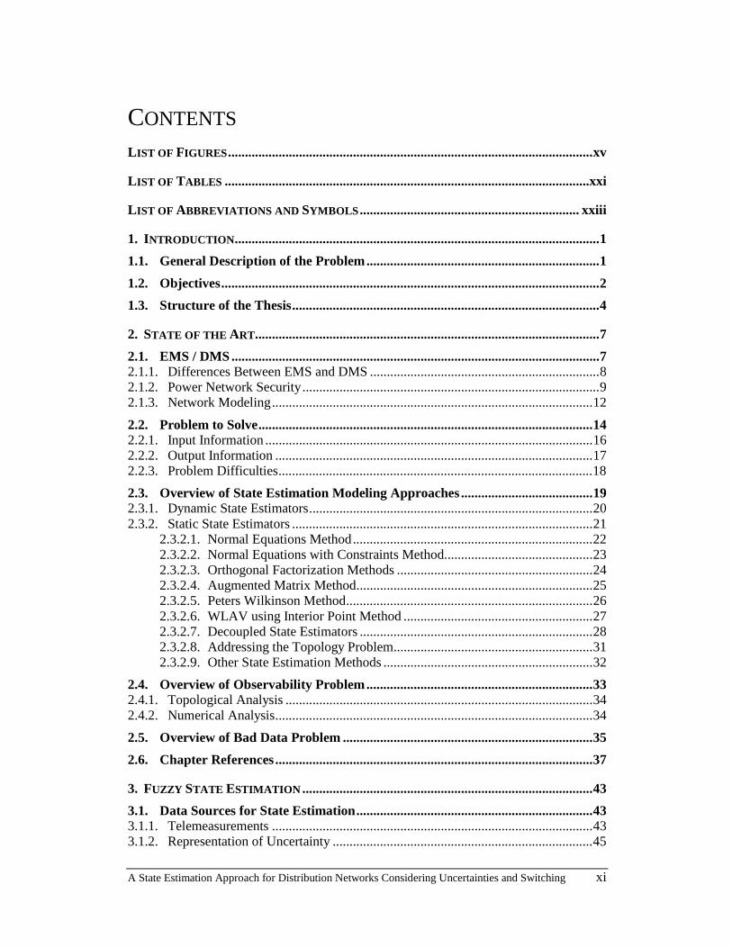
CONTENTS LIST OF FIGURES............................................................................................................xv
LIST OF TABLES ............................................................................................................xxi
LIST OF ABBREVIATIONS AND SYMBOLS................................................................. xxiii
1. INTRODUCTION............................................................................................................1
1.1. General Description of the Problem.....................................................................1
1.2. Objectives................................................................................................................2
1.3. Structure of the Thesis...........................................................................................4
2. STATE OF THE ART......................................................................................................7
2.1. EMS / DMS .............................................................................................................7 2.1.1. Differences Between EMS and DMS ....................................................................8 2.1.2. Power Network Security........................................................................................9 2.1.3. Network Modeling...............................................................................................12
2.2. Problem to Solve...................................................................................................14 2.2.1. Input Information .................................................................................................16 2.2.2. Output Information ..............................................................................................17 2.2.3. Problem Difficulties.............................................................................................18
2.3. Overview of State Estimation Modeling Approaches .......................................19 2.3.1. Dynamic State Estimators....................................................................................20 2.3.2. Static State Estimators .........................................................................................21
2.3.2.1. Normal Equations Method.......................................................................22 2.3.2.2. Normal Equations with Constraints Method............................................23 2.3.2.3. Orthogonal Factorization Methods ..........................................................24 2.3.2.4. Augmented Matrix Method......................................................................25 2.3.2.5. Peters Wilkinson Method.........................................................................26 2.3.2.6. WLAV using Interior Point Method ........................................................27 2.3.2.7. Decoupled State Estimators .....................................................................28 2.3.2.8. Addressing the Topology Problem...........................................................31 2.3.2.9. Other State Estimation Methods ..............................................................32
2.4. Overview of Observability Problem...................................................................33 2.4.1. Topological Analysis ...........................................................................................34 2.4.2. Numerical Analysis..............................................................................................34
2.5. Overview of Bad Data Problem ..........................................................................35
2.6. Chapter References..............................................................................................37
3. FUZZY STATE ESTIMATION ......................................................................................43
3.1. Data Sources for State Estimation......................................................................43 3.1.1. Telemeasurements ...............................................................................................43 3.1.2. Representation of Uncertainty .............................................................................45
Contents
xii A State Estimation Approach for Distribution Networks Considering Uncertainties and Switching
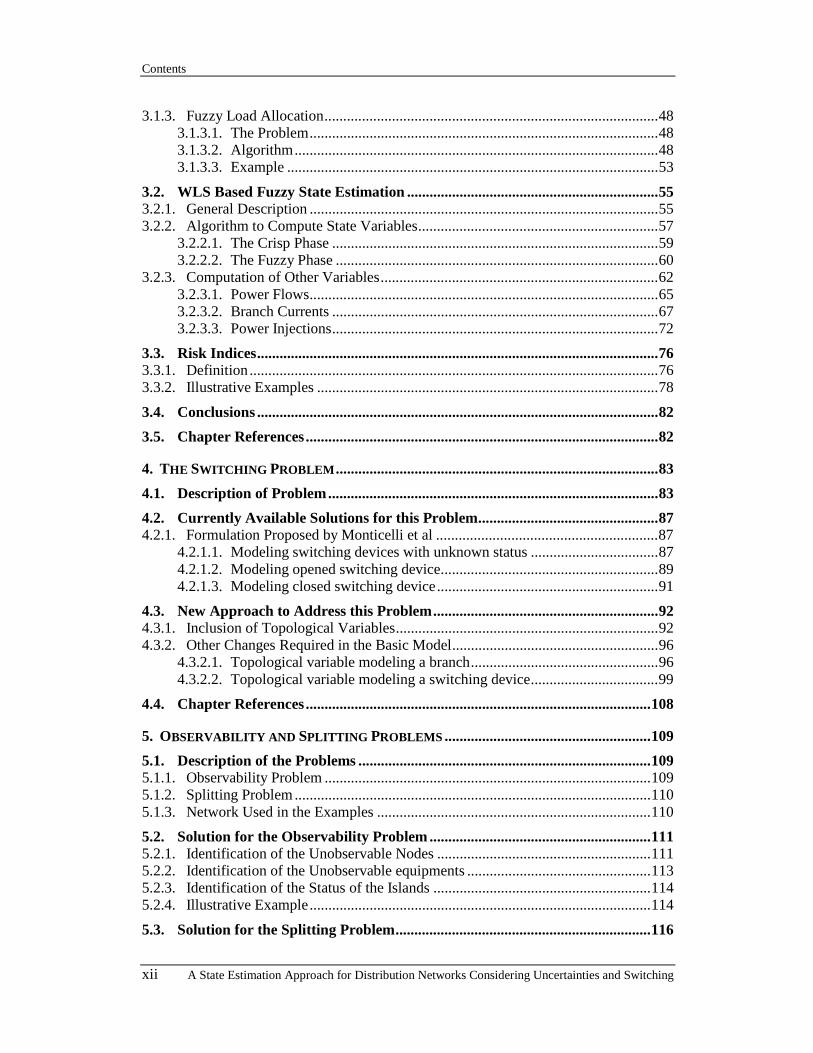
3.1.3. Fuzzy Load Allocation.........................................................................................48 3.1.3.1. The Problem.............................................................................................48 3.1.3.2. Algorithm.................................................................................................48 3.1.3.3. Example ...................................................................................................53
3.2. WLS Based Fuzzy State Estimation ...................................................................55 3.2.1. General Description .............................................................................................55 3.2.2. Algorithm to Compute State Variables................................................................57
3.2.2.1. The Crisp Phase .......................................................................................59 3.2.2.2. The Fuzzy Phase ......................................................................................60
3.2.3. Computation of Other Variables..........................................................................62 3.2.3.1. Power Flows.............................................................................................65 3.2.3.2. Branch Currents .......................................................................................67 3.2.3.3. Power Injections.......................................................................................72
3.3. Risk Indices...........................................................................................................76 3.3.1. Definition .............................................................................................................76 3.3.2. Illustrative Examples ...........................................................................................78
3.4. Conclusions ...........................................................................................................82
3.5. Chapter References..............................................................................................82
4. THE SWITCHING PROBLEM......................................................................................83
4.1. Description of Problem........................................................................................83
4.2. Currently Available Solutions for this Problem................................................87 4.2.1. Formulation Proposed by Monticelli et al ...........................................................87
4.2.1.1. Modeling switching devices with unknown status ..................................87 4.2.1.2. Modeling opened switching device..........................................................89 4.2.1.3. Modeling closed switching device...........................................................91
4.3. New Approach to Address this Problem............................................................92 4.3.1. Inclusion of Topological Variables......................................................................92 4.3.2. Other Changes Required in the Basic Model.......................................................96
4.3.2.1. Topological variable modeling a branch..................................................96 4.3.2.2. Topological variable modeling a switching device..................................99
4.4. Chapter References............................................................................................108
5. OBSERVABILITY AND SPLITTING PROBLEMS .......................................................109
5.1. Description of the Problems ..............................................................................109 5.1.1. Observability Problem .......................................................................................109 5.1.2. Splitting Problem ...............................................................................................110 5.1.3. Network Used in the Examples .........................................................................110
5.2. Solution for the Observability Problem ...........................................................111 5.2.1. Identification of the Unobservable Nodes .........................................................111 5.2.2. Identification of the Unobservable equipments .................................................113 5.2.3. Identification of the Status of the Islands ..........................................................114 5.2.4. Illustrative Example...........................................................................................114
5.3. Solution for the Splitting Problem....................................................................116

Contents
A State Estimation Approach for Distribution Networks Considering Uncertainties and Switching xiii
5.3.1. Formulation........................................................................................................116 5.3.2. Illustrative Example...........................................................................................118
5.4. Illustrative Examples .........................................................................................118 5.4.1. Case 1 - Two Energized Islands.........................................................................118 5.4.2. Case 2 - Two Energized Islands and One Isolated Island..................................120 5.4.3. Case 3 - System Initially Erroneously Splitted ..................................................121
5.5. Chapter References............................................................................................123
6. TUNING THE ALGORITHM WITH A FUZZY INFERENCE SYSTEM.........................125
6.1. Introduction........................................................................................................125
6.2. Fuzzy Inference Systems....................................................................................126
6.3. Use of a FIS to Find Weights.............................................................................130 6.3.1. General Aspects .................................................................................................130 6.3.2. Input Variables...................................................................................................131
6.3.2.1. Connectivity of the branch (RLAr) ........................................................132 6.3.2.2. Physical characteristics of the branch (RLAr/i) .....................................133 6.3.2.3. Voltage deviation level of the area (VoltageDLevel) ............................135 6.3.2.4. Load level of the extreme buses (LoadLevel) ........................................136 6.3.2.5. Significance of the load on the extreme buses (LoadRatio) ..................138
6.3.3. Output Variable and Training Set ......................................................................140 6.3.4. Rules Obtained...................................................................................................142
6.3.4.1. TS fuzzy system .....................................................................................142 6.3.4.2. Mamdani fuzzy system ..........................................................................146
6.4. Conclusions .........................................................................................................149
6.5. Chapter References............................................................................................149
7. APPLICATION OF THE DEVELOPED ALGORITHMS TO AN ILLUSTRATIVE NETWORK ................................................................................................................151
7.1. Illustrative Network...........................................................................................151 7.1.1. Network Used ....................................................................................................151 7.1.2. Available Measurements....................................................................................152 7.1.3. Observability Analysis.......................................................................................154
7.1.3.1. Adding qualitative information..............................................................154 7.1.3.2. Load Allocation procedure.....................................................................156
7.1.4. Topological Issues .............................................................................................158
7.2. Some Results .......................................................................................................161
7.3. Chapter References............................................................................................167
8. CONCLUSIONS..........................................................................................................169
8.1. General Conclusions ..........................................................................................169
8.2. Perspectives of Future Work.............................................................................171

Contents
xiv A State Estimation Approach for Distribution Networks Considering Uncertainties and Switching
A. BASIC CONCEPTS OF FUZZY SETS .........................................................................175
A.1. Some Definitions.................................................................................................175
A.2. Basic Operations on Fuzzy Sets ........................................................................176
A.3. Fuzzy Logic Operators ......................................................................................177 A.3.1. t-Norms and t-Conorms .....................................................................................177 A.3.2. Selection of the Aggregation Operators to Be Used ..........................................181
A.4. Fuzzy Numbers...................................................................................................182 A.4.1. Triangular Fuzzy Number..................................................................................182 A.4.2. Trapezoidal Fuzzy Number................................................................................183 A.4.3. Gaussian Fuzzy Number ....................................................................................184 A.4.4. LR Fuzzy Number..............................................................................................184
A.5. Extension Principle ............................................................................................185
A.6. Arithmetic Operations on Fuzzy Numbers......................................................186 A.6.1. Unary Operations ...............................................................................................186 A.6.2. Binary Operations ..............................................................................................187 A.6.3. Expressions to Perform in a Fast Way the Extended Arithmetic Operations
on Trapezoidal Fuzzy Numbers .........................................................................189
A.7. Ordering of Fuzzy Numbers .............................................................................194
A.8. Appendix References .........................................................................................195
B. DATA OF ILLUSTRATIVE NETWORKS ....................................................................197
B.1. IEEE 24 Bus Test System ..................................................................................197 B.1.1. Network Characteristics.....................................................................................197 B.1.2. Power Flow Results ...........................................................................................199
B.2. Augmented Network Based on the IEEE 24 Test System ..............................201 B.2.1. Network Characteristics.....................................................................................201 B.2.2. Power Flow Results ...........................................................................................204 B.2.3. Measurement Values for the Crisp State Estimation Phase...............................206 B.2.4. Rough Load Allocation......................................................................................209 B.2.5. Fuzzy State Estimation Results..........................................................................211
A State Estimation Approach for Distribution Networks Considering Uncertainties and Switching xv
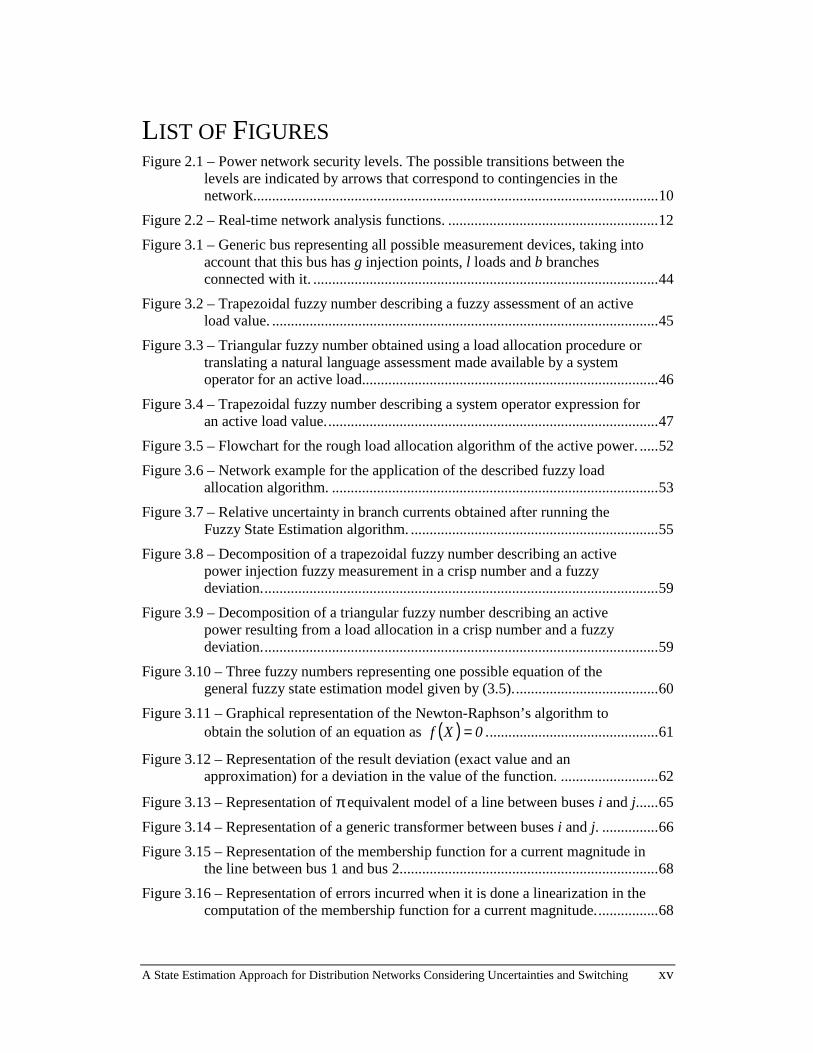
LIST OF FIGURES Figure 2.1 – Power network security levels. The possible transitions between the
levels are indicated by arrows that correspond to contingencies in the network............................................................................................................10
Figure 2.2 – Real-time network analysis functions. ........................................................12
Figure 3.1 – Generic bus representing all possible measurement devices, taking into account that this bus has g injection points, l loads and b branches connected with it. ............................................................................................44
Figure 3.2 – Trapezoidal fuzzy number describing a fuzzy assessment of an active load value. .......................................................................................................45
Figure 3.3 – Triangular fuzzy number obtained using a load allocation procedure or translating a natural language assessment made available by a system operator for an active load...............................................................................46
Figure 3.4 – Trapezoidal fuzzy number describing a system operator expression for an active load value.........................................................................................47
Figure 3.5 – Flowchart for the rough load allocation algorithm of the active power. .....52
Figure 3.6 – Network example for the application of the described fuzzy load allocation algorithm. .......................................................................................53
Figure 3.7 – Relative uncertainty in branch currents obtained after running the Fuzzy State Estimation algorithm. ..................................................................55
Figure 3.8 – Decomposition of a trapezoidal fuzzy number describing an active power injection fuzzy measurement in a crisp number and a fuzzy deviation..........................................................................................................59
Figure 3.9 – Decomposition of a triangular fuzzy number describing an active power resulting from a load allocation in a crisp number and a fuzzy deviation..........................................................................................................59
Figure 3.10 – Three fuzzy numbers representing one possible equation of the general fuzzy state estimation model given by (3.5).......................................60
Figure 3.11 – Graphical representation of the Newton-Raphson’s algorithm to obtain the solution of an equation as ( ) 0Xf = ..............................................61
Figure 3.12 – Representation of the result deviation (exact value and an approximation) for a deviation in the value of the function. ..........................62
Figure 3.13 – Representation of π equivalent model of a line between buses i and j......65
Figure 3.14 – Representation of a generic transformer between buses i and j. ...............66
Figure 3.15 – Representation of the membership function for a current magnitude in the line between bus 1 and bus 2.....................................................................68
Figure 3.16 – Representation of errors incurred when it is done a linearization in the computation of the membership function for a current magnitude.................68

List of Figures
xvi A State Estimation Approach for Distribution Networks Considering Uncertainties and Switching
Figure 3.17 – Representation of the membership functions of the real part and the imaginary part of the current in the line between bus 1 and bus 2..................69
Figure 3.18 – Representation of the membership curve (left side) and membership function (right side) representing the magnitude of the fuzzy complex value related to the current in the line between bus 1 and bus 2.....................70
Figure 3.19 – Representation of two rectangles in the complex plane defined by the real and the imaginary parts of the current in the line between bus 1 and bus 2, corresponding to the membership levels α = 0.0 and α = 1.0..............71
Figure 3.20 – Two possible membership functions for the current magnitude obtained from the real and the imaginary parts in the line between bus 1 and bus 2. ........................................................................................................72
Figure 3.21 – Representation of the membership function representing the corrected current magnitude in the line between bus 1 and bus 2. .................................72
Figure 3.22 – Representation of a power injection by a generator or a connection with another networks on bus i. ......................................................................74
Figure 3.23 – Representation of power consumption by one or more loads on bus i......76
Figure 3.24 – Representation of a generic power injection due to generation, connection to another networks or consumptions at bus i. .............................76
Figure 3.25 – Example of displaying the ORI value using colours for the line between buses i and j. .....................................................................................77
Figure 3.26 – Representation of the membership function for a current magnitude in branches with thermal limits equal to 560A and 500A...................................79
Figure 3.27 – Representation of the membership function for a current magnitude in branches with thermal limits equal to 440A and 600A...................................79
Figure 3.28 – Representation of a membership function for a bus voltage magnitude with admissible values between 0.9 and 1.1 p.u. in one case and between 0.9 and 1.0 p.u. in another case. ......................................................................80
Figure 3.29 – Representation of a membership function for a bus voltage magnitude with admissible values between 1.0 and 1.1 p.u. in one case and between 0.9 and 1.2 p.u. in another case. ......................................................................80
Figure 3.30 – Representation of a membership function example for a bus power injection magnitude with limit of 1100 MVA in one case and 1000 MVA in another case.................................................................................................81
Figure 4.1 – Application example of one heuristic rule with the purpose of finding or changing the network topology...................................................................84
Figure 4.2 – Application example of another heuristic rule having the purpose of finding or changing the network topology. .....................................................85
Figure 4.3 – Network to exemplify the usefulness the concept of extended island in the topology processor. ...................................................................................86
Figure 4.4 – Graph representing the network of Figure 4.3 using a conventional topology processor. .........................................................................................86
List of Figures
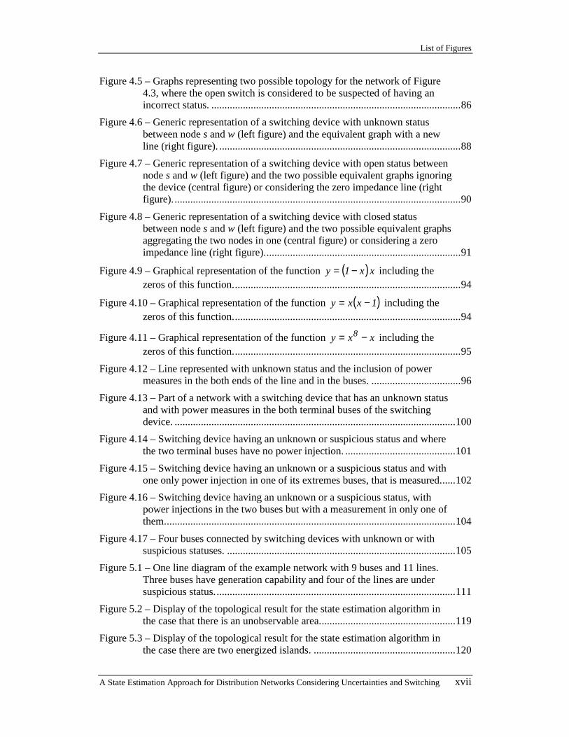
A State Estimation Approach for Distribution Networks Considering Uncertainties and Switching xvii
Figure 4.5 – Graphs representing two possible topology for the network of Figure 4.3, where the open switch is considered to be suspected of having an incorrect status. ...............................................................................................86
Figure 4.6 – Generic representation of a switching device with unknown status between node s and w (left figure) and the equivalent graph with a new line (right figure). ............................................................................................88
Figure 4.7 – Generic representation of a switching device with open status between node s and w (left figure) and the two possible equivalent graphs ignoring the device (central figure) or considering the zero impedance line (right figure)..............................................................................................................90
Figure 4.8 – Generic representation of a switching device with closed status between node s and w (left figure) and the two possible equivalent graphs aggregating the two nodes in one (central figure) or considering a zero impedance line (right figure)...........................................................................91
Figure 4.9 – Graphical representation of the function ( )xx1y −= including the zeros of this function.......................................................................................94
Figure 4.10 – Graphical representation of the function ( )1xxy −= including the zeros of this function.......................................................................................94
Figure 4.11 – Graphical representation of the function xxy 8 −= including the zeros of this function.......................................................................................95
Figure 4.12 – Line represented with unknown status and the inclusion of power measures in the both ends of the line and in the buses. ..................................96
Figure 4.13 – Part of a network with a switching device that has an unknown status and with power measures in the both terminal buses of the switching device. ...........................................................................................................100
Figure 4.14 – Switching device having an unknown or suspicious status and where the two terminal buses have no power injection. ..........................................101
Figure 4.15 – Switching device having an unknown or a suspicious status and with one only power injection in one of its extremes buses, that is measured......102
Figure 4.16 – Switching device having an unknown or a suspicious status, with power injections in the two buses but with a measurement in only one of them...............................................................................................................104
Figure 4.17 – Four buses connected by switching devices with unknown or with suspicious statuses. .......................................................................................105
Figure 5.1 – One line diagram of the example network with 9 buses and 11 lines. Three buses have generation capability and four of the lines are under suspicious status............................................................................................111
Figure 5.2 – Display of the topological result for the state estimation algorithm in the case that there is an unobservable area....................................................119
Figure 5.3 – Display of the topological result for the state estimation algorithm in the case there are two energized islands. ......................................................120

List of Figures
xviii A State Estimation Approach for Distribution Networks Considering Uncertainties and Switching
Figure 5.4 – Display of the topological result for the state estimation algorithm in the case there are two energized islands and one isolated island. .................121
Figure 5.5 – Display of the example network result from the state estimation algorithm and with a single island including the 11 nodes. ..........................122
Figure 6.1 – Generic representation of an intelligent system that for some values for the input variables gives a weight as output..................................................126
Figure 6.2 – Schematic diagram of a FIS with the different blocks. .............................126
Figure 6.3 – Neural visual arrangement of a FIS, that has two input variables with three fuzzy values for each variable. .............................................................127
Figure 6.4 – Graphical representation of a Gaussian membership function with two parameters, m and d . ..................................................................................128
Figure 6.5 – Display of the network used to illustrate the definition of the FIS. ..........131
Figure 6.6 – Graphical representation of the five Gaussian membership functions related with the fuzzy input variable RLAr (Relation between the branch conductance and the average of the two terminal buses conductance). ........133
Figure 6.7 – Graphical representation of the five Gaussian membership functions related with the fuzzy input variable RLAr/i (Relation between the branch conductance and the branch susceptance).....................................................134
Figure 6.8 – Graphical representation of the five Gaussian membership functions related with the fuzzy input variable VoltageDLevel (average of the two differences for the nominal voltage in the terminal buses). ..........................136
Figure 6.9 – Graphical representation of the five Gaussian membership functions related with the fuzzy input variable LoadLevel (average of the active power consumption in the two terminal buses). ...........................................138
Figure 6.10 – Graphical representation of the five Gaussian membership functions related with the fuzzy input variable LoadRatio (relation between the LoadLevel and the total of the active power consumption in all island buses). ...........................................................................................................139
Figure 6.11 – Graphical representation of the seven Gaussian membership functions related with the fuzzy output variable weight for a Mamdani fuzzy system............................................................................................................142
Figure 6.12 – Fuzzy Inference System that for values of the five input variables gives as result a weight to be associated to the topological variable to obtain good results. .......................................................................................142
Figure 6.13 – Example of application of one rule and the membership function for the consequent variable obtained by application of this rule to line 8 of the network in Figure 6.5. .............................................................................147
Figure 6.14 – Membership function after the OR operation in the consequent variables obtained by application of 10 rules to line 8 of the used example. ........................................................................................................148
Figure 7.1 – Augmented network based on the IEEE 24 buses network with a new voltage level at 30 kV. ..................................................................................151

List of Figures
A State Estimation Approach for Distribution Networks Considering Uncertainties and Switching xix
Figure 7.2 – Generic representation of a fuzzy measurement with a triangular membership function.....................................................................................155
Figure 7.3 – Representation of a sub-network with 14 buses where the fuzzy load allocation algorithm was ran. ........................................................................157
Figure 7.4 – Representation of the buses 14 and 16 modelled at the section level. ......159
Figure 7.5 – Representation of the buses 15 and 24 modelled at the section level. ......160
Figure 7.6 – Membership functions for the measurements and for the results of the voltage magnitude in the buses 11 and 14. ...................................................162
Figure 7.7 – Membership functions for the results of the voltage phase in the buses 11 and 14.......................................................................................................163
Figure 7.8 – Membership functions for the measurements and for the results of the active and reactive power injected on bus 50................................................163
Figure 7.9 – Membership functions for the measurements and for the results of the active and reactive power injected on bus 48................................................164
Figure 7.10 – Membership functions for the measurements and for the results of the active and reactive power injected on bus 40................................................164
Figure 7.11 – Membership functions for the measurements and for the results of the active and reactive power flow on the branch connecting buses 18 and 21..165
Figure 7.12 – Membership functions for the measurements and for the results of the active and reactive power flow on the branch connecting buses 29 and 32..165
Figure 7.13 – Membership functions for the results of the active and reactive power load on bus 32. ..............................................................................................165
Figure 7.14 – Membership functions for the results of the current on the branches 26-29 and 49-50. ...........................................................................................166
Figure A.1 – Membership functions for two fuzzy sets, one is convex (left function) and the other is non convex (right function). ................................................176
Figure A.2 – Membership function for a triangular fuzzy number................................183
Figure A.3 – Membership function for a trapezoidal fuzzy number. ............................183
Figure A.4 – Membership function for a Gaussian fuzzy number. ...............................184
Figure A.5 – Left and right removals of à regarding the real number k......................194
Figure B.1 – IEEE 24 bus Test System. ........................................................................197
Figure B.2 – Augmented network based on the IEEE 24 bus network with a new voltage level at 30 kV. ..................................................................................202


A State Estimation Approach for Distribution Networks Considering Uncertainties and Switching xxi
LIST OF TABLES Table 3.1 – Values for the parameters used to run the rough load allocation
algorithm for all the LV substations of ENERGY type. .................................54
Table 3.2 – Values obtained from the rough load allocation algorithm for all the LV substations.......................................................................................................54
Table 6.1 – Values for the parameters m and d of the five Gaussian membership functions related with the fuzzy input variable RLAr...................................133
Table 6.2 – Values for the parameters m and d of the five Gaussian membership functions related with the fuzzy input variable RLAr/i.................................135
Table 6.3 – Values for the parameters m and d of the five Gaussian membership functions related with the fuzzy input variable VoltageDLevel....................136
Table 6.4 – Values for the parameters m and d of the five Gaussian membership functions related with the fuzzy input variable LoadLevel. ..........................138
Table 6.5 – Values for the parameters m and d of the five Gaussian membership functions related with the fuzzy input variable LoadRatio. ..........................140
Table 6.6 – Some points used in the training set for the FIS.........................................141
Table 6.7 – Some rules obtained after the training process by an ANFIS for a TS fuzzy system..................................................................................................143
Table 6.8 – Values for weights obtained for each rule and the respective firing strength, for line 8 of the illustrative example. .............................................144
Table 6.9 – Some rules obtained after the training process by an NEFPROX for a Mamdani fuzzy system. ................................................................................146
Table 7.1 – Values for the measurements obtained from the measurement devices in the buses. They are also indicated the zero values for the buses having zero injection and zero values for possible voltage phase references. ..........153
Table 7.2 – Values for the measurements obtained from the measurement devices installed in the branches of the augmented network. ....................................153
Table 7.3 – Values for the fuzzy measurements of the power injection and voltage magnitude in buses obtained from the operator information or from historical data. ...............................................................................................155
Table 7.4 – Values for the fuzzy measurements of the power flow in branches obtained from the historical data, using a load forecast algorithm. ..............156
Table 7.5 – Values for the parameters used to run a fuzzy load allocation for all the loads on sub-network of Figure 7.3...............................................................157
Table 7.6 – Values for the pseudo-measurements obtained from the load allocation for all the loads on sub-network of Figure 7.3. .............................................158
Table 7.7 – Values for the input variables of the FIS and the weight obtained with this system for the topological variables. ......................................................161
Table A.1 – Some t-norms and the respective function ( ).t . .........................................178

List of Tables
xxii A State Estimation Approach for Distribution Networks Considering Uncertainties and Switching
Table A.2 – Some t-conorms (or s-norms) and the respective function ( ).s . ................179
Table A.3 – Typical dual pairs of t-norms and t-conorms (or s-norms). .......................180
Table B.1 – Characteristics of the buses of the IEEE 24 bus Test System....................198
Table B.2 – Characteristics of the branches of the IEEE 24 bus Test System. .............199
Table B.3 – Power flow results for the buses of the IEEE 24 bus Test System. ...........200
Table B.4 – Power flow results for the branches of the IEEE 24 bus Test System. ......201
Table B.5 – Characteristics of the buses of the augmented network that are different from IEEE 24 bus Test System. ....................................................................203
Table B.6 – Characteristics of the branches of the augmented network that are different from IEEE 24 bus Test System. .....................................................204
Table B.7 – Power flow results for the buses of the augmented network. ....................205
Table B.8 – Power flow results for the branches of the augmented network. ...............206
Table B.9 – Measurement values and respective weights in the buses of the augmented network. These can be the value of the measurement device or the central value of the fuzzy assessment. ....................................................208
Table B.10 – Measurement values in the branches of the augmented network. These can be values of the measurement device or central values of a fuzzy assessment.....................................................................................................209
Table B.11 – Values for the parameters used to run the fuzzy load allocation algorithm for all the loads on the feeders included in the IEEE 24 bus network..........................................................................................................210
Table B.12 – Values for the pseudo-measurements obtained from the load allocation algorithm for the loads on the feeders included in the IEEE 24 bus network. ..................................................................................................211
Table B.13 – Values of the fuzzy results of the Fuzzy State Estimation obtained for the voltages in the buses of the augmented network.....................................213
Table B.14 – Values of the fuzzy results of the Fuzzy State Estimation obtained for the power injections in the buses of the augmented network........................214
Table B.15 – Values of the fuzzy results of the Fuzzy State Estimation obtained for the power and current flows in the branches of the augmented network. .....216

A State Estimation Approach for Distribution Networks Considering Uncertainties and Switching xxiii
LIST OF ABBREVIATIONS AND SYMBOLS A – ampere (current unit)
ANFIS – Adaptive Neuro-Fuzzy Inference System
ANN – Artificial Neural Network
DMS – Distribution Management System
EMS – Energy Management System
FIS – Fuzzy Inference System
GIS – Geographical Information System
IRLS – Iteratively Reweighted Least Squares
kV – kilovolt (voltage unit - V 10kV 1 3= )
LAV – Least Absolute Value
LMS – Least Median of Squares
LV – Low Voltage
MV – Medium Voltage
MVA – mega-voltampere (power unit - VA 10MVA 1 6= )
Mvar – megavar (reactive power unit - var 10Mvar 1 6= )
MW – megawatt (active power unit - W10MW 1 6= )
NEFPROX – Neuro Fuzzy Function Aproximator
OPF – Optimal Power Flow
ORI – Overload Risk Index
P ij – expression to evaluate the active power flow in the branch between buses i and j
p.u. – per unit
Q ij – expression to evaluate the reactive power flow in the branch between buses i and j
rad – radian (angle unit)
RTU – Remote Telemetry Unit
SCADA – System Control and Data Acquisition
TS – Takagi-Sugeno
TSK – Takagi-Sugeno-Kang
V – volt (voltage unit)
VA – voltampere (power unit)
var – reactive power unit

List of Abbreviations and Symbols
xxiv A State Estimation Approach for Distribution Networks Considering Uncertainties and Switching
W – watt (active power unit)
WLAV – Weighted Least Absolute Value
WLS – Weighted Least Squares

A State Estimation Approach for Distribution Networks Considering Uncertainties and Switching 1
1. INTRODUCTION
1.1. GENERAL DESCRIPTION OF THE PROBLEM In recent years, the electricity sector is facing several changes and challenges related to new legal and regulatory frameworks, to the explosion of dispersed generation and to larger pressures to increase quality of service. In distribution networks these challenges are perhaps even more evident clearly requiring larger investments on automation and telemetering devices as well as in the installation of more powerful control centres. This move determines the need to develop new methodologies and models to cope with specific characteristics of distribution networks.
The general problem addressed by the research described in this Thesis is the State Estimation problem in electrical networks. The electrical networks can be transmission networks, distribution networks or systems integrating both transmission and distribution networks. The State Estimation problem can be described as aiming at finding the values for a set of variables (state variables) that adjust in a more adequate way to a set of network values (measurements) that are available. The state variables are such that all the other network variables can be evaluated from them. The calculation of state variables considers the physical laws directing the operation of electrical networks and is typically done adopting some criterium.
This is not a complex problem if the number of network measurements is large, well distributed among the network and free of errors. However, in some networks the number of network measurements is reduced, there are some areas in the network where it does not exist any measurement and the available ones can be affected by errors or can even be incomplete. Therefore, for a system with these characteristics, the State Estimation turns into a challenge. In this Thesis we will solve this problem by using all the information available for the network, not only measurement values. Of course, the quality of the solution turns better as the quality of the available information improves.
In fact, measurements can be affected by errors, related to the quality of measurement devices or due to transmission deficiencies. Time skew problems are also an important issue when trying to install state estimation codes in control centres. In fact, due to the characteristics of the communication systems used to link the control centre with the substations, the set of measurements available at a certain instant will generally correspond to different sampling instants. This is not a so serious problem if the system is operating in steady state conditions and if the topology of the network does not change, but it contributes to increase the incoherence that usually affects the available measurements. However, if a topology change occurred or if a load or generation strongly changed, time skew problems can have a large impact on the results.
The research described in this Thesis lead to new contributions in the area of State Estimation algorithms specially conceived to be run in the control centres of distribution networks. These are the networks where the referred problems are more frequent. It should be emphasised that our main concern is to turn feasible the application of State Estimation algorithms in a real time industrial environment. This concern comes from recognising that theoretical contributions frequently fail in their ability to be implemented in real systems. This concern lead to a hybridisation between traditional

Chapter 1. Introduction
2 A State Estimation Approach for Distribution Networks Considering Uncertainties and Switching
probabilistic State Estimation approaches and fuzzy set models specially devoted to capture the uncertainty that may affect the knowledge of some injections in distribution networks. The treatment of practical implementation issues was also motivated by the integration of this software module, as well as other application functions, in a DMS - Distribution Management System.
During several years traditional vertically integrated utilities directed large parts of their budgets to the generation/ transmission areas leading to high levels of automation and telecontrol. This means that until recently State Estimation studies were performed essentially in generation/transmission control centres. On the other hand, distribution networks remained till recently as the poor part of the systems thus having much lower levels of quality of service, automation and telecontrol capabilities.
In recent years, the increase of dispersed generation connected to distribution networks, the accent on the overall requirements of service quality, the move to consider electricity as a commodity in the scope of the implementation of market mechanisms as well as new regulatory and tariff schemes pressed companies to direct larger parts of their budgets to the distribution sector. Therefore, power systems are experiencing substantial changes from organisational, regulatory and technological points of view. To a certain extent, these advances enabled the introduction of competition and the generalisation of market mechanisms in America, Europe and Australia turning feasible and less costly several solutions that previously were impossible to consider.
The new way of facing distribution activities imposed a new accent on upgrading existing SCADA – System Control and Data Acquisition – systems to more powerful systems turning them into real DMS systems. These new systems, to a certain extent, adopt some characteristics present in EMS - Energy Management System. However, the migration of EMS software to distribution control centres can not be done directly given the particularities of this sector.
SCADA systems allowed the operators to have a graphic vision of the networks including real time available measurements, to implement in a remote way several control actions on switching devices, transformers, capacitors and other equipment. However, the database of those systems was very incomplete in the sense that it was not possible to have a mathematical model of the system able to support more complex power system functions like the power flow and short circuit analysis, contingency, fault identification or service restoration. Besides other functions as topology processor, the development of State Estimation algorithms directed to distribution networks can be integrated in this move aiming at transforming SCADA systems into powerful DMS systems.
1.2. OBJECTIVES In the Thesis, we present an integrated approach to solve the State Estimation problem specially intended to be used in DMS. The presented methodology is a hybrid model that uses various types of data as deterministic (network and topology information), fuzzy (load curves for low voltage substations and other qualitative information) and probabilistic (measurements values). Using this model, we are also addressing the state estimation observability problem, since in distribution networks the number available measurements is usually reduced. Therefore, in distribution networks historic databases are usually poor so that pseudo-measurements based on them are difficult to obtain.

1.2. Objectives
A State Estimation Approach for Distribution Networks Considering Uncertainties and Switching 3
The main objectives of the proposed approach are the following ones:
−−−− The developed model should be able to deal with networks having a reduced number of real time measurements and a reduced degree of automation. Due to the size of distribution networks, the amount of required investments to increase telemetering is large. This means that in the next years the use of traditional State Estimation algorithms will not be possible. If one wants to run State Estimation models now, new approaches will have to be adopted to solve this problem;
−−−− It should integrate qualitative descriptions modelled by fuzzy sets regarding loads or injections, namely based on characteristic load curves. In this scope, fuzzy loads can be characterised using a load allocation methodology;
−−−− It should integrate qualitative information or knowledge about types of consumers. Moreover, it should incorporate data about installed capacity and power and energy consumptions of some loads. These information can be also useful to define fuzzy loads by using a load allocation methodology;
−−−− Another objective is the integration of current measurements, as these are the most frequent measures taken in distribution networks. In the load allocation methodology, these current measurements, if needed, can be converted into active and reactive power flows by using a specified power factor or a default value;
−−−− Power flows or average powers should be estimated as, in several cases, tariff schemes adopted to remunerate companies for the use of their distribution networks in the scope of the move to competition are based on them. This opens new fields of application of State Estimation algorithms also contributing to turn them more crucial in control centres since their results can directly determine the flow of money between several entities;
−−−− It should be considered that distribution networks general have poor levels of quality of service and that switching strategies are frequently adopted to restore the supply of electricity in several areas. The adoption of these strategies can also be imposed by the possibility of changing of supplier in the scope of the move to the market and by the penalties imposed to companies if quality indices are not met;
−−−− These strategies also mean that distribution networks are not so stable from a topological point of view as transmission ones. The action of switching devices lead to topology changes regarding which there may exist uncertainty on the control centre. This means the operator, depending on the automation and telecontrol levels, may not be sure about the topology of the system in operation. Apart from this, considering a fixed and constant topology for the network is not a valid assumption any more. This means that the developed algorithm must address this issue. In this case, this problem was treated by considering variables corresponding to the state - opened or closed - of circuit breakers, together with the available information;
−−−− It should be solved the convergence difficulties related with the influence of topological variables on the convexity of the surface associated to the error
Chapter 1. Introduction
4 A State Estimation Approach for Distribution Networks Considering Uncertainties and Switching
function of the State Estimation problem. This can be addressed by adequately selecting the weights assigned to each relation associated to the topological variables. This will be important to soften the surface to be analysed and therefore to improve the convergence of the State Estimation algorithm;
−−−− Admitting some degree of uncertainty affecting the current status of switching devices means that one should also consider the possibility of system splitting. That is, splitting in several islands can, in some cases, be much more adequate in order to explain the available measured values. On the contrary, there may occur situations in which the initial number of islands is large but a more reduced one is more adequate to better explain the available measurements. The developed algorithm must be flexible enough to incorporate splitting in several islands or merging several of them;
−−−− The algorithm should be able to run for networks with a large size. This requires the adoption of efficient models and techniques. This means that networks having a larger size impose new challenges on real time applications. This dimensional problem is also an important characteristic of distribution networks.
Considering all these concerns and objectives, in this Thesis we aim at presenting an integrated State Estimation model that incorporates solutions and techniques to deal with the previously referred questions.
1.3. STRUCTURE OF THE THESIS The concerns and objectives referred previously lead to this text in which, apart from this introductory chapter, there are 7 chapters and two appendices. In each of them they are indicated the used References.
In Chapter 2 of this Thesis we detail the main factors determining the current move to achieve higher levels of automation and telecontrol in distribution networks as well as the main issues that have to be addressed when passing from EMS systems to DMS. Moreover, we characterise State Estimation modules in the scope of DMS (or EMS) applications and we stress the importance of these modules on the security analysis of electric networks. Additionally, it is formulated the State Estimation problem, considering different possibilities for the input and output data, and they are identified the difficulties inherent to this problem. Afterwards, they are present the main approaches available in the literature to deal with this problem. At the end of Chapter 2 they are briefly described the observability and bad data analysis sub-problems, as well as some approaches to deal with these issues.
In Chapter 3 we characterise the sources of data to be used by several application functions and particularly by State Estimation algorithms focused in distribution networks. In this scope, it is described the Fuzzy Load Allocation algorithm that allow us to obtain data affected by uncertainty in some areas where there are not other available information. This Chapter also describes the developed State Estimation algorithm including the incorporation of uncertain measures modelled by fuzzy concepts. This algorithm is based in the Weighted Least Squares algorithm traditionally used in State Estimation. In this formulation they are included expressions to evaluate the results for all network variables, including current flows for which, in some cases, a

1.3. Structure of the Thesis
A State Estimation Approach for Distribution Networks Considering Uncertainties and Switching 5
corrective procedure must be run. Moreover, it is defined the Overload Risk Index - ORI - that can be useful in order to characterise the ability of the system to accommodate the specified uncertain injections without violating branch limits or voltage ranges.
In Chapter 4 we present a new approach to address the lack of knowledge regarding the topology in operation. This approach is based on the integration of topological variables having a continuous nature. However, the inclusions of some equations on the model impose constraints to these topological variables such that the solution for them will be binary.
In Chapter 5 we present the observability and the splitting problems, and the solution developed for them. In the solution to be presented, the State Estimation algorithm runs in the entire network and the unobservable parts are identified only at the end. The splitting problem is related with the fact that the number of islands at the beginning of the State Estimation algorithm described in this Thesis can be different from the number of islands at the end. Therefore, in this Chapter, it is described a novel way to deal with this problem.
In Chapter 6 we present an inference system that, for a set of values for five input variables, generates weights to be associated to topological variables. This set of values is obtained based on the characteristics of buses and branches near the device or branch with suspicious or unknown status. This inference system will be created based in the experience obtained from running small examples and saving the results from each one of these examples. Thus, a large number of small examples are run with topological variables with unknown status or with suspicious status. The inference system, based on a large number of small examples, is then used to obtain the weights to assign to topological variables in larger size problems.
In Chapter 7 we finally present a case study based on the IEEE 24 bus Test System to illustrate the developed methodology. The IEEE 24 bus Test System was modified by adding some feeders in the scope of a new voltage level in order to represent distribution networks.
Chapter 8 presents some relevant conclusions of the research work. They are also presented some perspectives of future work related with the problems and methodologies that were address and developed.
This Thesis ends with two Appendices. Appendix A presents some basic concepts of Fuzzy Sets required to better understand the Fuzzy State Estimation algorithm. Appendix B presents the network used for illustrative purposes in Chapter 7. As this network is based on the IEEE 24 bus Test System, it is previously presented this network and afterwards they will be detailed the modifications as used in Chapter 7. For these two networks they are presented all data needed to run a power flow exercise and, in the second case, they are also indicated all the data needed to run the State Estimation algorithm.


A State Estimation Approach for Distribution Networks Considering Uncertainties and Switching 7
2. STATE OF THE ART
2.1. EMS / DMS During several years in the past electrical utilities were organized in traditional vertically integrated structures and directed large parts of their investment budgets to the generation / transmission areas leading to high levels of automation and telecontrol in these subsystems. This control is performed by using a package called EMS - Energy Management System which includes real time applications that continuously monitor the network. On the other side, distribution networks remained till recently as the poor part of the system thus having much lower levels of quality of service, automation and telecontrol capabilities.
In recent years, the accent on the overall requirements of service quality, the move to consider electricity as a commodity in the scope of the implementation of market mechanisms as well as new regulatory and tariff schemes pressed companies to direct larger parts of their budgets to the distribution sector. In this scope, the traditional SCADA – System Control and Data Acquisition systems are being upgraded to more powerful systems that, to a certain extent, adopt some characteristics present in EMS to distribution networks. However, this migration of EMS software to distribution control centres cannot be done directly given the particularities of this sector. In this scope, reference [1] presents some recent developments achieved by Kokai, Masuda, Horiike and Sekine, in the EMS and in the SCADA, in particular the application of the open systems technology.
Power systems are recently experiencing substantial changes from organizational, regulatory and technological points of view. These changes are strongly related in the sense that one of the driving forces of the re-regulation of power systems is the advances in communication, computer science and applications specially directed to power systems. To a certain extent, these advances enabled from a technical point of view the introduction of competition and the generalization of market mechanisms in America, Europe and Australia turning feasible and less costly solutions that previously were impossible to consider.
The re-regulation of power systems transforms the state estimation from an important application into a critical one. Several transmission network utilities are being merged into larger regional systems and also with independent system operators (ISO) leading to transmission system operators (TSO). Power transfers now take place over larger electrical distances and in directions for which the networks were not originally designed. Competitive and monetary factors become the main drivers of the process, provided that the electrical operating limits are not violated. As the transmission and distribution networks have finite capacities, the system operator has to assume management decisions that must be equitable, considering security concerns and addressing network congestion. These decisions may curtail or refuse power transfer rights, and this has a critical financial significance.
The liberalization trend started in the generation subsector and large consumers (considered eligible consumers) leading to wholesale electricity markets but soon spread to distributors and retailers turning more independent the paths responsible for the flow

Chapter 2. State of the Art
8 A State Estimation Approach for Distribution Networks Considering Uncertainties and Switching
of money and for the flow of electricity. The creation of more business opportunities, which is associated with larger risks, was balanced by a larger emphasis on quality of service leading to the need to monitor and control not only transmission networks but also, most of all, distribution ones.
The automation of distribution networks was also motivated and determined by the liberalization of the ownership of small generation and the incentives to install cogeneration plants as a way to use endogenous and, in many cases, renewable resources. This liberalization occurred in many countries prior to the re-regulation and, to a certain extent, it could be seen as a first step in this move that contributed to reduce the role of traditional utilities. The presence of a large number of those plants in traditionally poorly automated distribution networks required the monitorization of distribution systems and pressed utilities to invest in automation and in installing the first generation of SCADA systems.
These systems allowed the operators to have a graphic vision of the networks including real time available measurements, to implement in a remote way several control actions on switching devices, transformers, capacitors and other controlled equipments. However, the database of those systems was very incomplete in the sense that it was not possible to have a mathematical model of the system able to support more complex power system functions as state estimation, power flow and short circuit and contingency analysis, fault identification or service restoration. The inclusion of these modules required the enlargement of the existing databases and that several new issues had to be addressed if some applications were to migrate from well developed EMS existing in generation / transmission control centres to distribution systems.
2.1.1. DIFFERENCES BETWEEN EMS AND DMS
As it was referred before, there are some issues to have in mind when studying and performing the migration of the well developed EMS existing in generation / transmission control centres to the recently developed control systems of distribution networks. These issues include the following main aspects:
−−−− In generation / transmission systems there is a sufficiently large number of real time measurements leading to an acceptable redundancy level in terms of state estimation algorithms. This level of redundancy is very important in the sense that some measurements can have large errors, and some others are not measured or not telemetered. This means that using other measurements it is possible to obtain estimates of these ones. This is a direct consequence of the investments that for many years were directed to generation / transmission systems leading to high levels of automation, telecontrol capabilities and quality of service;
−−−− On the contrary, in distribution networks the number of real time measurements and the degree of automation is traditionally reduced leading to the impossibility of directly install and run EMS state estimation modules. In this kind of networks there is no redundancy and it frequently happens that in some parts of the network there are no available information in real time;
−−−− Another major issue is related with the curse of dimensionality. In fact, distribution networks are much larger than transmission ones turning it more
2.1. EMS / DMS
A State Estimation Approach for Distribution Networks Considering Uncertainties and Switching 9
demanding the use of any algorithm in real time. This means that distribution networks are usually very large and when supervision systems are used in regional networks (including generation / transmission networks and also distribution networks) the EMS / DMS can be specified to run in acceptable time for networks having as much as 100 000 buses;
−−−− Distribution networks traditionally have poor levels of quality of service leading to the adoption of frequent switching strategies to restore the supply of electricity in several areas. The adoption of these strategies is also imposed by the possibility of changing of supplier in the scope of the move to the market and by the penalties imposed to companies if quality indices are not met. These strategies also mean that distribution networks are not so stable from a topological point of view as transmission ones. The action of switching devices lead to frequent topology changes regarding which there may exist uncertainty in the control center. This means the operator, depending on the automation and telecontrol levels, may not be sure about the complete topology of the system in operation;
−−−− Tariff schemes that are adopted to remunerate companies for the use of their distribution networks, in the scope of the move to competition, are often based on flows of energy or on average powers. This means that these values have to be measured or have to be estimated in some way. This opens new fields of application of state estimation algorithms also contributing to turn them more crucial in control centers since their results can directly determine the flow of money between several entities.
These concerns impose new challenges to the industrial and research communities leading to new levels of collaboration and to hybrid models and applications often combining traditional approaches with emerging techniques. This evolution is finally leading to applications more adapted to the characteristics of distribution networks called DMS – Distribution Management Systems – in an analogy to already existing EMS systems. The DMS packages must deal with the distribution network problems as the problems in the regional networks that involve one or more distribution networks and a generation / transmission network.
2.1.2. POWER NETWORK SECURITY
In the both systems, EMS and DMS, there is a network security requirement that is one of main objectives of the supervision of the network by these applications. The concept of network security is related with the probability of maintaining an adequate supply of power while not violating several operating and technical constraints. The higher security level is related with a lower probability of loss of load. On the other hand, a lower security level is related with a higher probability of loss of load. This means, that the control actions are directed to maintaining the security level higher, therefore avoiding blackouts and equipment damage.
A contingency is related to a loss of transmission equipment or generation units. The analysis of the possible contingencies that can occur and the detection of the potential destructive ones is called Contingency Analysis. This definition means that the possible contingencies that would lead the system into a state of emergency should be analyzed.

Chapter 2. State of the Art
10 A State Estimation Approach for Distribution Networks Considering Uncertainties and Switching
One contingency can involve only a single equipment outage or multiple (two or more) equipment outages.
When an insecure contingency case happens in a system, the system enters in an alert level in which there are two basic possible responses:
−−−− The first is a preventive procedure consisting of the modification of the state before the occurrence of the contingency in order to eliminate the potential damages if the contingency really occurs;
−−−− The other is a corrective procedure and it consists of the definition and implementation of a control strategy to deal with the emergency state after the contingency and in the case that it occurs.
The basic methodology for security analysis was created by Dy Liacco and it is described in reference [2]. The functions for an economy-security control and an optimal power flow including contingency constraints and preventive control actions were discussed by Stott, Alsaç, and Monticelli in reference [3]. In the reference [4] by Monticelli are presented these issues and in particular the classification of the power network security levels, as they are reproduced in Figure 2.1.
NoncorrectableEmergency
CorrectableEmergency
CorrectivelySecure
Alert
Secure
Restorative
Level 1
Level 2
Level 3
Level 4
Level 5
Level 6
Figure 2.1 – Power network security levels. The possible transitions between the levels are indicated by arrows that correspond to contingencies in the network.
Figure 2.1 presents six security levels that can occur in power systems. These levels are required to define control actions in a preventive procedure or in a corrective procedure. These security levels are:
−−−− Secure (level one) - a system at this level has all the loads supplied without violating operating limits. If one contingency occurs the system remains operating without violating its limits. This means that, in this level, when one

2.1. EMS / DMS
A State Estimation Approach for Distribution Networks Considering Uncertainties and Switching 11
of the possible contingencies occurs the system doesn't need any corrective procedure because no emergency state is reached with only one contingency;
−−−− Correctively Secure (level two) - in the same way as in the previous level, a system at this level has all the loads supplied without violating operating limits. However, if a contingency occurs the operating limits violations are not a problem, in terms of loss of loads, since control actions are taken to correct them in a little time step. This level is more economic than level one, but it relies on actions taken after contingencies and performed by the EMS / DMS. Nevertheless, the risk of emergency is greater for a system operating in this level when compared with operating in level one. The adequate control actions can be identified in advance by running an optimal power flow with security constraints and including pos-contingency rescheduling;
−−−− Alert (level three) - in the same way as in the previous two levels, a system at this level has all the loads supplied without violating operating limits. However, violations due to some contingencies cannot be corrected without load curtailment. The system can be brought back to level one or to level two by preventive rescheduling using an optimal power flow (OPF) with security constraints;
−−−− Correctable Emergency (level four) - a system at this level has all the loads supplied but some operating limits are violated and these violations can be corrected without performed load curtailment. The system can be brought back to level three by performing corrective actions;
−−−− Noncorrectable Emergency (level five) - in the same way as in the previous level, a system at this level has all the loads supplied but some operating limits are violated. However, these violations cannot be corrected without load curtailment. The amount, the type and the location of the load curtailment can be optimized by an optimal power flow (OPF) program. This optimization is important because the curtailment of some loads is more critical than others. For instance, loosing the supply of an hospital loads is far more critical than the curtailment of public lights;
−−−− Restorative (level six) - a system at this level has no violations in the operating limits but some load curtailment has occurred. When the system is in this level the control action required attempts to return the system back to level one or to level two.
The determination of the current security level of a system and the appropriate control action to be taken at each level are carried out by the various EMS / DMS economy--security functions. These economy-security functions involve the integrated use of network monitoring, contingency analysis and optimal power flow, as described in reference [4] and represented in the Figure 2.2. All these functions have in common the need to know the current system state provided by the state estimator process. This is a traditional and decoupled vision of state estimation and topology process. As it will be referred in the sequence, there are several methodologies aiming at integrating these two issues.
The EMS / DMS runs real-time processes designed to maintain a specified security level at minimum operational cost. While operating a system at a pre-defined security level
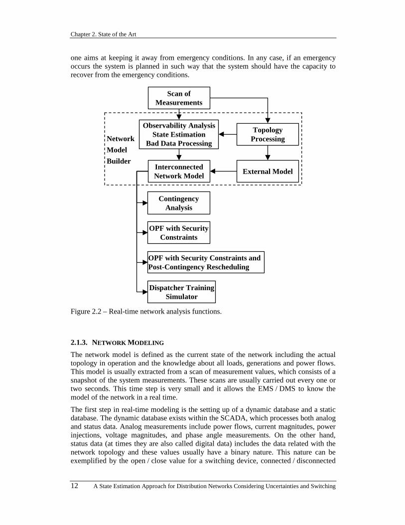
Chapter 2. State of the Art
12 A State Estimation Approach for Distribution Networks Considering Uncertainties and Switching
one aims at keeping it away from emergency conditions. In any case, if an emergency occurs the system is planned in such way that the system should have the capacity to recover from the emergency conditions.
Network
Model
BuilderInterconnectedNetwork Model
External Model
TopologyProcessing
Observability AnalysisState Estimation
Bad Data Processing
Scan ofMeasurements
ContingencyAnalysis
OPF with SecurityConstraints
OPF with Security Constraints andPost-Contingency Rescheduling
Dispatcher TrainingSimulator
Figure 2.2 – Real-time network analysis functions.
2.1.3. NETWORK MODELING
The network model is defined as the current state of the network including the actual topology in operation and the knowledge about all loads, generations and power flows. This model is usually extracted from a scan of measurement values, which consists of a snapshot of the system measurements. These scans are usually carried out every one or two seconds. This time step is very small and it allows the EMS / DMS to know the model of the network in a real time.
The first step in real-time modeling is the setting up of a dynamic database and a static database. The dynamic database exists within the SCADA, which processes both analog and status data. Analog measurements include power flows, current magnitudes, power injections, voltage magnitudes, and phase angle measurements. On the other hand, status data (at times they are also called digital data) includes the data related with the network topology and these values usually have a binary nature. This nature can be exemplified by the open / close value for a switching device, connected / disconnected

2.1. EMS / DMS
A State Estimation Approach for Distribution Networks Considering Uncertainties and Switching 13
for a generator or a load, in service / out of service for a line or a transformer. The static database contains the fixed information for the network like the equipment parameters (lines impedances, transformer impedances, …) and the configuration data (connections between the equipments). If it is possible to evaluate the state variables with the available data in the two databases, the network is considered observable.
The different steps needed to build the network model, after performing the scan of measurements by the SCADA, are represented in the top of the Figure 2.2. There are several different methodologies to treat these steps. However, we can identify some common points to all of them. Furthermore, there is a conventional methodology for the state estimation where almost all the others are based, which was developed by Schweppe and co-authors presented in references [5], [6] and [7]. The expression State Estimation can be considered in a wide meaning since it can involve not only the evaluation algorithm but also the entire network model builder.
Conventional state estimation is performed on a bus / branch model of the same type of the one that is used in power flow calculations. However, the network configuration is described in the static database in terms of connections between bus sections and switching devices, and between switching devices and lines or transformers. This level of representation of the network is called Physical Level. The network topology processor, using the status data in the dynamic database, is used to convert the physical level representation in the bus / branch model.
In the conventional topology processor the bus / branch model is built before the state estimation process as well as the other functions like the observability analysis and bad data processing. This means, it is assumed that is possible to know the topology and that this topology is considered to be correct beyond any doubt. The bad data processing only looks at analog data to identify large errors. Therefore, the network model builder can be divided in two distinct main data processors. One data processor is for the status data, it is run in the first place and it consists of the network topology processor. Another data processor is for the analog data, it is composed of the observability analysis, state estimation and bad data processing, and it uses the bus / branch model build by the first data processor.
An important issue when the EMS / DMS builds the network model is related with interconnections with other systems that are not included under this control system responsibility, and that are adjacent networks affecting the state of the network under control. For instance, topology changes such as line or generation outages in the nearby networks can have a significant effect on the controlled system. Therefore, in order to improve the ability to monitor and securely operate the network, the information about the system operation of the neighboring electrical systems is highly required.
The network controlled by the EMS / DMS will be called Internal System (usually one simply uses power system to refer to this system) and the others interconnected networks are called External Systems. The External Systems can be replaced by equivalent networks or they can be maintained in the unreduced form. Nevertheless, the best approach to adopt is a compromise between the unreduced model, for a part of the each adjacent network, and the reduced equivalent used for the remainder of each network.
There are three main approaches to build the model for the interconnected systems:

Chapter 2. State of the Art
14 A State Estimation Approach for Distribution Networks Considering Uncertainties and Switching
−−−− The power flow technique - in this method the external model is attached to the internal model by the inclusion of the corresponding boundary injections. These injections are calculated by solving a power flow for the external network while treating the boundary buses as swing buses. The voltage values in these buses are obtained by state estimation in the Internal System. These buses totally absorb the possible errors existing on the assumptions of network topology and power injections for the External System. The Internal System is correctly reproduced by this method, but the errors can affect the contingency analysis and optimal power flow studies because the reactions of the external model to the internal changes may be incorrect. Incorporation of telemetered branch flow data is difficult in this method, although generator reactive power limits and voltage limits enforcement may be implemented. Some applications using this approach were developed by Deckmann, Pizzolante, Monticelli, Stott and Alsaç in references [8] and [9];
−−−− The state estimation technique with one-pass - in this method one single state estimation is run for the whole network (internal and external). In this method, one must be careful to avoid any contamination of the effects of bad data from the External into the Internal System. In addition, enforcement of generator reactive power limits and voltage limits at controlled buses may be accomplished. An application using this approach was developed by Monticelli and Wu in reference [10];
−−−− The state estimation technique with two-passes - in this method state estimation is used to produce an initial estimate of the Internal System state. The external model is then attached in two passes. In the first pass, an initial power flow is used, as in the first approach, to evaluate branch power flows in the unobservable network. In the second pass, state estimation runs using the estimated states in the Internal System as pseudo-measurements and the evaluated power flows for the External System. Any real-time telemetry available from the External System can be effectively used by state estimation in the second pass. An application using this approach was developed by Bose in reference [11].
Some other mixed methodologies have been presented to deal with the external network modeling like the one presented in reference [12] by Lu, Liu and Vemuri. In this reference it is presented a method that combines the power flow technique and the state estimation technique described in the previous paragraphs. This method is based in a two stage solution approach: stage one simulates the external data using a power flow; and stage two runs a state estimation on the external network model in order to refine it.
A critical review of external system modeling was presented in reference [13] by Wu and Monticelli. More recently the state of the art in the external network model topic was reviewed by the IEEE Task Force on External Network Modeling, chaired by Kato and the resulting work is presented in reference [14].
2.2. PROBLEM TO SOLVE As discussed in the previous sections, the state estimator is used to build the model for the network under analysis together with results that can be used to build models for external connected networks. If the system has an appropriate redundancy level (ratio
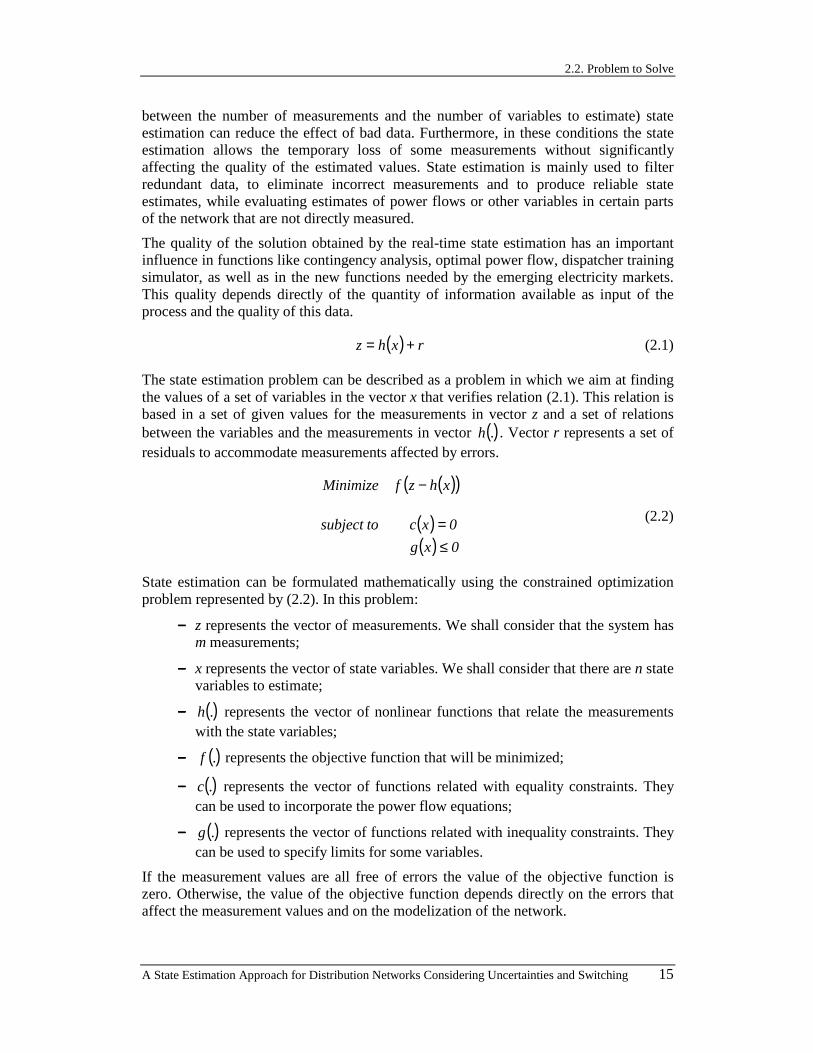
2.2. Problem to Solve
A State Estimation Approach for Distribution Networks Considering Uncertainties and Switching 15
between the number of measurements and the number of variables to estimate) state estimation can reduce the effect of bad data. Furthermore, in these conditions the state estimation allows the temporary loss of some measurements without significantly affecting the quality of the estimated values. State estimation is mainly used to filter redundant data, to eliminate incorrect measurements and to produce reliable state estimates, while evaluating estimates of power flows or other variables in certain parts of the network that are not directly measured.
The quality of the solution obtained by the real-time state estimation has an important influence in functions like contingency analysis, optimal power flow, dispatcher training simulator, as well as in the new functions needed by the emerging electricity markets. This quality depends directly of the quantity of information available as input of the process and the quality of this data.
( ) rxhz += (2.1)
The state estimation problem can be described as a problem in which we aim at finding the values of a set of variables in the vector x that verifies relation (2.1). This relation is based in a set of given values for the measurements in vector z and a set of relations between the variables and the measurements in vector ( ).h . Vector r represents a set of residuals to accommodate measurements affected by errors.
( )( )
( )( ) 0xg
0xcto subject
xhzfMinimize
≤=
−
(2.2)
State estimation can be formulated mathematically using the constrained optimization problem represented by (2.2). In this problem:
−−−− z represents the vector of measurements. We shall consider that the system has m measurements;
−−−− x represents the vector of state variables. We shall consider that there are n state variables to estimate;
−−−− ( ).h represents the vector of nonlinear functions that relate the measurements with the state variables;
−−−− ( ).f represents the objective function that will be minimized;
−−−− ( ).c represents the vector of functions related with equality constraints. They can be used to incorporate the power flow equations;
−−−− ( ).g represents the vector of functions related with inequality constraints. They can be used to specify limits for some variables.
If the measurement values are all free of errors the value of the objective function is zero. Otherwise, the value of the objective function depends directly on the errors that affect the measurement values and on the modelization of the network.

Chapter 2. State of the Art
16 A State Estimation Approach for Distribution Networks Considering Uncertainties and Switching
2.2.1. INPUT INFORMATION
The input information for the state estimation process obviously corresponds to all values in the related static database for the area in which one wants to estimate the network model. The data in this static database can comprise some elements, or in general all the elements, of the following list:
−−−− Set of all equipment included in the analysed area. This includes a set of buses, lines, transformers, generators, loads, capacitor banks, switching devices as well as their physical characteristics. These characteristics can be, for instance, the impedances, the nominal current, the length and other information for each line, or the magnetizing admittances, the windings connection type, the type of the tap, the available tap positions if the tap can be changed, the winding impedances, the nominal apparent power and other information for each transformer;
−−−− Connections between the terminals of all the elements. This information includes only the physical connections between the elements and not the status of the equipment that has manoeuvre capability. This means that, for instance, if a switching device has one terminal in one line and the other in one bus, these two equipments are connected even if the switching device has the opened status at a certain moment. At this point it is not possible to know the information included in the dynamic database that is updated in a real-time mode. On the contrary, this kind of information is obtained in a off-line mode before starting the process.
The state estimation function estimates a set of variables based in a set of measurements and pseudo-measurements of different types. These measurements are preserved dynamically and on-line in the dynamic database referred in the previous section. The different types of measurements are:
−−−− Voltage magnitude measurement in one bus or indicated value for the voltage magnitude in case it is considered as a pseudo-measurement;
−−−− Voltage angle measurement in one bus or indicated value for the voltage angle if it is considered as a pseudo-measurement;
−−−− Active power injection measurement in one bus or indicated value for the active power injection. This active power injection specification can be done by the system operator, or by another function used to predict power injection values like a load allocation function or a load forecast function;
−−−− Reactive power injection measurement in one bus or indicated value for the reactive power injection. This reactive power injection specification can also be indicated by the system operator, or by another function used to predict power injection values like a load allocation function or a load forecast function;
−−−− Injected current magnitude measurement in one bus or indicated value for the injected current magnitude. This value can also be indicated by the system operator, or by another function used to predict current values like a load allocation function or a load forecast function;

2.2. Problem to Solve
A State Estimation Approach for Distribution Networks Considering Uncertainties and Switching 17
−−−− Active power flow measurement in one branch (line, group of lines or transformer) or other available value for this flow used as pseudo--measurement;
−−−− Reactive power flow measurement in one branch (line, group of lines or transformer) or other available value for this flow used as pseudo--measurement;
−−−− Current magnitude flow measurement in one branch (line, group of lines or transformer) or other available value for this flow used as pseudo--measurement;
−−−− Switching device status measurement in a switching equipment (switcher, breaker, fuse, sectionaliser, switch-fuse, sectionaliser-fuse, …) or specified as pseudo-measurement by the system operator;
−−−− Magnitude of the tap measurement in one transformer winding or an available value used as pseudo-measurement;
−−−− Phase shifter angle measurement in one transformer winding or an available value used as pseudo-measurement;
−−−− Reactive power injection measurement by a capacitor bank at the nominal voltage, in the connection bus of the network, or an available value used as pseudo-measurement.
All these information can be used if necessary. If the redundancy level is large, the state estimation process can ignore the measurements that have lower quality. This means that, for instance, in a system having a redundancy level equal to two there may be available two measurements for the same load value. One of these values is obtained by the SCADA with a good quality and the other value is obtained by qualitative information provided by the operator. The state estimation, in general, uses only the measured value. However, it is possible that an error occurs with this value and then the other one can be used to replace the first one.
2.2.2. OUTPUT INFORMATION
The output of the state estimator is a complete description of the current network model for all the observable areas of the analysed network. This also means that the unobservable areas are identified. There must exist consistency between the solution obtained for observable and initially declared unobservable areas of the network. In particular there cannot be mismatches at the boundaries of those areas. The areas previously referred as unobservable are treated as observable ones after including all available pseudo-measurements.
The current network model can be obtained from a complete voltage solution, magnitudes and phases for all buses in the network under analysis, together with the topology status. An easy test to the process consists of using as input a set of measurements completely free of errors. With these values, the state estimator must provide a solution that corresponds to the solution of a traditional power flow study. This means that the results for the variables used as measurements must coincide with the values used as inputs.

Chapter 2. State of the Art
18 A State Estimation Approach for Distribution Networks Considering Uncertainties and Switching
The outputs of the state estimation process can be all of the following values or only some to take into account eventual simplifications:
−−−− Status of the switching devices with unknown status or with wrong status as input;
−−−− Identification of the buses and branches integrating unobservable areas;
−−−− Voltages magnitude values for each bus in the observable areas;
−−−− Voltage angle values for each bus in the observable areas;
−−−− Active and reactive injected power on each bus in the observable areas;
−−−− Reactive power injections by each capacitor bank in the observable areas;
−−−− Active and reactive power consumption by each load in the observable areas;
−−−− Active and reactive power generation by each generator or group of generators in the observable areas;
−−−− Transformer tap and phase shift for each transformer for the transformers having these devices, in the observable areas;
−−−− Active and reactive power flows in the extremities of each branch in the observable areas;
−−−− Current flows and power factors in the extremities of each branch in the observable areas;
−−−− Set of measurements and pseudo-measurements that were used to estimate the computed values;
−−−− Set of measurements and pseudo-measurements that were identified as being affected by larger errors;
−−−− Normalised residuals for all the used measurements;
−−−− Confidence index for the computed solution.
These values are all the desirable values that an EMS / DMS should deliver as output of the state estimator. However, some available methodologies are able to evaluate all these variables, and some of them assume some variables as having fixed values in the input data.
2.2.3. PROBLEM DIFFICULTIES
As it was seen, if there were no errors in the input data the state estimator should have no problems to converge to the correct solution. However, the input data is affected by different type of errors that must be filtered by the state estimator. These errors happen as a consequence of one or more than one of the following factors:
−−−− Error of the measurement equipment, usually called Remote Telemetry Unit (RTU). These errors can be due to noise or malfunction of the equipment that causes the loss of the measured value;

2.3. Overview of State Estimation Modeling Approaches
A State Estimation Approach for Distribution Networks Considering Uncertainties and Switching 19
−−−− Error on the communication of the measured value from the RTU to the control center;
−−−− Calibration errors in the RTU. These errors are generally represented in the mathematical model by random variables considered has having a certain probabilistic distribution. However, the adopted distribution can also be affected by errors;
−−−− Synchronization problems related with the instant on time when the values are acquired. In some cases the values are not obtained simultaneously in the time. This issue is usually known as time skew problem and means that a state estimator is run using measured values from different states;
−−−− Some values can be obtained during a perturbation like a short-circuit, for instance. These are transient states that may not be adequately sampled to be fully characterized by a state estimation procedure;
−−−− Asymmetries on the system related with an unbalanced situation between the three phases;
−−−− Errors on the equipment parameters of the static database, that can be a consequence of an error in the introduction of these values;
−−−− Errors in the mathematical model, that can be due to an incorrect validation of the model or a consequence of an arrangement between some questionable factors for the model;
−−−− Topological errors due erroneous status data stored in the dynamic database. These errors can result from errors in the SCADA or errors due to the operator knowledge of the operation conditions given that he may believe that a status is correct while being, in fact, incorrect;
−−−− Pseudo-measurements data obtained from other functions that generally are not completely correct. Some of these functions give as results not a single value but a range of possible values;
−−−− Pseudo-measurements data specified by the operator using his knowledge and experience. These may be not completely correct, apart from being eventually specified in terms of a range of possible values.
This list of problems that can affect the values of the input data is very extensive. This means that some of these errors affect the input data and so the solution can be affected by some errors that must be minimized by the state estimator. If they are not completely eliminated, the algorithm must filter, as much as possible, the good from the bad input data.
2.3. OVERVIEW OF STATE ESTIMATION MODELING APPROACHES There are two different approaches to deal with the state estimation problem. In one of them, the system is considered static while in the other it is assumed dynamic. In the first case, the algorithms handle with a time invariant case in which state estimated values are evaluated from a single scan of measurements. This is the approach that will be discussed in a more detailed way in this Thesis. In the second set of approaches, the
Chapter 2. State of the Art
20 A State Estimation Approach for Distribution Networks Considering Uncertainties and Switching
algorithms consider the time evolution of the system and aim at dealing with multiple scans of measurements.
2.3.1. DYNAMIC STATE ESTIMATORS
The algorithms that address the dynamic state estimation problem to evaluate the state variables use a sequence of measurements through time. The time is defined as a discrete variable and it is increased considering a time step. This approach uses a model like (2.3) to describe the scan of measurements at instant it and a model (2.4) to
describe the dynamic state vector overtime. In these models:
−−−− ( )itz represents the vector of measurement values corresponding to instant it ;
−−−− ( ).h is the vector of nonlinear functions;
−−−− ( )itx is the state vector at instant it ;
−−−− ( )ite is the error vector at instant it with zero mean and assumed to be not
correlated through time;
−−−− ( )itv is the vector including changes on the state vector from instant 1it − to it .
It is assumed that they also are zero mean random variables not correlated through time.
( ) ( )( ) ( )iii tetxhtz += (2.3)
( ) ( ) ( )i1ii tvtxtx += − (2.4)
The algorithms aiming at solving the dynamic state estimation problem can be classified in three groups:
−−−− Tracking State Estimator - this algorithm does not make assumptions about the time behavior of the state vector. This means, that this algorithm only uses the equation (2.3) of the dynamic model;
−−−− Linear Dynamic State Estimator, which uses the Kalman Filter technique to describe the dynamic behavior of the system. These algorithms make a linearization in the measurement model, using the linear model (2.5) instead of using equation (2.3). In this equation ( )itH represents the Jacobian matrix of
( ).h at instant it ;
( ) ( ) ( ) ( )iiii tetxtHtz += (2.5)
−−−− Non-Linear Dynamic State Estimator, which can be solved using the Kalman Bucy Filter technique to describe the dynamic behavior of the system. The algorithms of this group use the nonlinear model and adopt a successive linearization strategy.
A solution approach for the dynamic state estimation problem was proposed by Leite da Silva, Coutto Filho and Cantera in reference [15]. This solution incorporates the main

2.3. Overview of State Estimation Modeling Approaches
A State Estimation Approach for Distribution Networks Considering Uncertainties and Switching 21
advantages of the tracking estimators and the dynamic estimators. This algorithm is used to facilitate the detection and identification of bad data.
A critical review of the main developments in dynamic state estimation was presented in 1990 by Rousseaux, Van Cutsem and Dy Liacco in reference [16]. More recently, some algorithms have been proposed to deal with the problem of the dynamic state estimation as, for instance, the solutions proposed by Sinha and Mondal in reference [17] and by Gou and Abur in reference [18]. The algorithm described in reference [17] incorporates a short term load forecasting module using Artificial Neural Networks (ANN) to obtain a realistic dynamic model for the prediction step. This method solves the problem of the non-linear dynamic state estimation. The Tracking State Estimator algorithm presented in reference [18] is intended to monitor power system operation under nonsinusoidal periodic steady state conditions. This estimator is based on the discrete time equations of the power system and it uses system wide synchronously sampled branch current and bus voltage measurements at regular intervals.
The complexity related with this type of modelization leads to several simplifications in the models and the algorithms. In this way, these types of algorithms are seldom used in control systems. On the contrary, the static state estimation based algorithms are the most popular and applied ones in the DMS / EMS commercial packages.
2.3.2. STATIC STATE ESTIMATORS
The general mathematical model that must be solved by the state estimator corresponds to the optimization problem represented by formulation (2.2). This optimization problem includes equality and inequality constraints, and it is generally called constrained state estimation. This optimization problem can be solved using the Weighted Least Squares (WLS) method. In this case, the equality constraints can be used to represent target values included in the model as pseudo-measurements. The inequality constraints are used to represent limits in the unobservable parts of the network.
The WLS method applied to the static state estimation problems in power systems based on the bus / branch model was introduced by Schweppe in references [5], [6] and [7]. Much research on these methods was developed since then aiming at finding better methods to solve large least square problems. The WLS method is the best estimator in the maximum likelihood sense when the errors have Gaussian nature, but it does not exhibit an inherent capability of filtering bad data. There are essentially four different methods to solve the WLS problem: the normal equations method, the orthogonal transformation method, the augmented matrix method and the Peters and Wilkinson method (also called by pseudo-inverses method).
A comparison of some of these approaches was presented by Holten, Gjelsvik, Aam, Wu, and Liu in reference [19]. The methods that are compared are the normal equations method, orthogonal transformation methods, hybrid methods of the two previous ones, normal equations with constraints method, and Hatchel's augmented matrix method. These methods are compared in terms of their numerical stability, computational efficiency and implementation complexity.
Another way to solve the optimization problem (2.2) corresponds to use the Weighted Least Absolute Value (WLAV) method. This type of estimators has been used
Chapter 2. State of the Art
22 A State Estimation Approach for Distribution Networks Considering Uncertainties and Switching
essentially given the good quality in filtering bad data. It can be solved using linear programming methods, like the simplex method, or an interior point approach.
Reviews of the state of the art in state estimation algorithms based on this modeling approaches were made by Bose and Clements in reference [20] and by Wu and Monticelli in reference [21]. A comprehensive bibliography on state estimation from 1968-1989 was prepared by Coutto Filho, Leite da Silva and Falcão and it was presented in reference [22].
2.3.2.1. Normal Equations Method
In the WLS method, the objective function is defined as a quadratic function according to expression (2.6). In this expression, W represents the matrix of weights and index T represents the transpose of a matrix or vector. This matrix of weights is assumed diagonal and for the telemetered variables, the elements of the diagonal of W usually correspond to the inverse of the variances of error measurement.
( )( ) ( )( ) ( )( )xhzWxhzxhzf T −−=− (2.6)
The resulting optimization problem can be solved by a numerical method such as the Newton-Raphson Method. This is clearly the most widely used approach to solve this problem. This numerical method is applied in terms of finding the zeros of the derivatives of the performance index ( )xJ , represented by expression (2.7). The
stationary conditions of (2.7) lead to the set of equations (2.8). In these expressions jjW
represents the diagonal element of the row j of the matrix of weights and m represents the number of elements of the measurements vector.
( )( ) ( )( ) ( )( )[ ] Wxhz2
1xhzWxhz
2
1J(x)
m
1jjj
2jj
T ∑=
−=−−= (2.7)
( )( ) 0.0x
(x)hWxhz
x
J(x) m
1j
jjjjj =
∂
∂−−=
∂∂ ∑
= (2.8)
Another numerical method used to solve the optimization problem (2.2) is the Gauss--Newton Method. This method involves the transformation of the original optimization problem into a linear least squares problem by linearizing the vector of functions ( )xh . If the Newton-Raphson Method is formulated in terms of only using the first derivatives in the Taylor Series of the function under analysis, the two numerical methods have the same iterative expression to update the state vector. This expression is represented by (2.9). The importance of second order derivatives in the Newton-Raphson Method in dealing with the presence of erroneous data was emphasized by Van Amerongen in the reference [23].
( )[ ] ( )[ ] ( )[ ] ( )xZWxHxWHxHx T1T ∆∆−
= (2.9)

2.3. Overview of State Estimation Modeling Approaches
A State Estimation Approach for Distribution Networks Considering Uncertainties and Switching 23
The method that solves the state estimation problem using the WLS method and using a numerical method like the Newton-Raphson Method is usually designated as the Normal Equations Method.
The numerical performance of the normal equations approach can be negatively affected by the presence of injection measurements, by the use of large weighting factors, and by the presence of very low impedance branches. These problems are related to the fact that
the gain matrix ( ) ( )[ ] ( )xWHxHxG T= is obtained by squaring the Jacobian matrix
( )xH , which makes the condition number worse. Most of the methods developed to improve the numerical robustness of the WLS estimators are thus designed to deal with this squaring problem.
The condition number is defined as the norm of a matrix times the norm of its inverse. The norm used can be one-norm or two-norm, and this condition number can be associated to all state estimation matrices. The smallest condition number for a matrix is one. Small values (below 100) generally indicate good conditioning and few numerical difficulties. Large values (greater than 100) indicate ill-conditioning. Multiplying a matrix by itself squares its condition number. Therefore, methods that rely on the explicit computation of the gain matrix are likely to be ill-conditioned, and this is designated as the squaring problem.
2.3.2.2. Normal Equations with Constraints Method
In the previous formulation, the equality constraints that appear in the WLS optimization problem (2.2) are included as pseudo-measurements by assigning them large weights. In this case, the optimization problem is solved using a Langrangian function to accommodate the equality constraints. Therefore, the inclusion of pseudo--measurements to represent these constraints is not required. The problem to be solved is now represented by (2.10).
( ) ( )( ) ( )( )( ) 0xcto subject
xhzWxhz2
1xJMinimize T
=
−−= (2.10)
This problem can be solved using the Langrangian function (2.11). ( )λ,xL should now be differentiated to obtain the Karush-Kuhn-Tucker first order necessary conditions for an optimal solution, yielding a system of nonlinear equations (2.12). In these equations
( ).H and ( ).C are Jacobian matrices. These nonlinear equations can be solved by a numerical method like the Gauss-Newton method.
( ) ( )( ) ( )( ) ( )xcxhzWxhz2
1,xL TT λλ −−−= (2.11)
( ) ( ) ( )( ) ( )( ) ( ) 0xc
,xL
0xCxhzWxHx
,xL T
=−=∂
∂
=−−−=∂
∂
λλ
λλ
(2.12)
Chapter 2. State of the Art
24 A State Estimation Approach for Distribution Networks Considering Uncertainties and Switching
In the reference [24] Aschmoneit, Peterson and Adrian propose a method that solves the state estimation problem using this approach. In the proposed algorithm, the equality constraints are used to represent the zero injections.
2.3.2.3. Orthogonal Factorization Methods
The use of orthogonal transformation methods to solve the WLS problem in the static state estimation of power systems was introduced by Simões Costa and Quintana in references [25] and [26]. The orthogonal transformations are based on the Householder transformation in the first reference and the Givens Rotations in the second one.
This type of methods solves the WLS constrained state estimation (2.2) by linearizing, with respect to a system operating point x, the vectors of nonlinear functions ( ).h , ( ).c
and ( ).g . In this case, the problem to be solved is represented by (2.13). In this
optimization problem, ( ).H , ( ).C and ( ).G are the Jacobian matrices, ( )xhzz −=∆ ,
( )xc0b −=∆ , ( )xg0d −=∆ and the x∆ can be used to update the state variable values. This update process can correspond to an iteration of the least-squares problem solved through Givens Rotations.
( ) ( )( ) ( )( ) ( )( )( ) dxxG
bxxCto subject
xxHWzWxxHzWxxHzxJMinimize2½½T
∆∆∆∆
∆∆∆∆∆∆∆
≤=
−=−−= (2.13)
The orthogonal transformation method avoids squaring the gain matrix by using a decomposition of the Jacobian matrix according to (2.14). This decomposition consists
of finding an orthogonal matrix Q (defined as having the propriety: IQQT = ) and an
upper trapezoidal matrix U ( 1U is a triangular matrix).
==0
UQUQHW 1TT½ (2.14)
The objective function ( )xJ ∆ of the problem (2.13) is then transformed according to (2.15). In this sequence two new vectors resulting from expression (2.16) are used.
( ) ( )
22
211
21
2
1
2½2½½
yxUyx0
U
y
y
xUzQWxxHQWzQWxJ
∆∆∆∆∆∆
∆∆∆∆∆
+−=
−
=
=−=−=
(2.15)
zQWy
y ½
2
1 ∆∆∆
=
(2.16)

2.3. Overview of State Estimation Modeling Approaches
A State Estimation Approach for Distribution Networks Considering Uncertainties and Switching 25
The minimum of the above objective function ( )xJ ∆ occurs when the expression (2.17) is verified and this coincides with the problem to be solved.
xUy 11 ∆∆ = (2.17)
Another method to solve the state estimation problem corresponds to a hybrid approach that solves the normal equations (2.9) using the orthogonal transformation only in the gain matrix. This transformation is given by expression (2.18). This method was proposed by Monticelli, Murari and Wu in reference [27].
( )[ ] ( ) ( )[ ] ( ) 1T
1T½T½T UUUUxHWxHWxWHxHG ==== (2.18)
Efficient sparse vector / matrix techniques based on Givens Rotation and the various advances made in speeding up the orthogonalization in the state estimation were achieved by Vempati, Slutsker and Tinney and they were presented in references [28] and [29]. Orthogonal sparse vector methods can be used to speed up processing sparse vectors in an orthogonal estimator by following factorization paths that skip nonessential operations. This is especially advantageous to compute the impact of small changes departing from a previously solved subproblem. Therefore, sparse vector methods can be used for partial reorthogonalization.
Recently, Pires, Simões Costa and Mili presented in reference [30] the application of the orthogonal transformation through the Givens Rotations to solve estimators based on the iteratively reweighted least squares (IRLS). The IRLS method is widely used in linear regression and its convergence properties are well known in Statistic applications. The first application of this method to the state estimation in power systems was done by Mili, Cheniae, Vichare and Rousseeuw in reference [31].
2.3.2.4. Augmented Matrix Method
This type of methods can be used to solve state estimation problems without and with constraints. If it does not include constraints, the problem to be solved is represented by (2.19). This problem can be solved using the augmented equations represented in matrix notation by (2.20).
( ) ( )( ) ( )( )xxHzWxxHzxJ Minimize T −−= (2.19)
( )( )[ ]
( )( )
=
−
−
0
z
x
xxHzW
0xH
xHWT
1 (2.20)
The augmented method requires that the computations are properly organized. There are many possibilities for doing that and the selection of the most adequate one to be used depends on the application. Once, this algorithm is started many of the diagonal elements in the augmented matrix are zero or very small, so that it is not possible to select diagonal pivots in an arbitrary way. There are three possibilities of doing this selection. In the first one, perform diagonal pivoting but defer the selection of an element as a pivot until its numeric value becomes sufficiently large. In the second one,
Chapter 2. State of the Art
26 A State Estimation Approach for Distribution Networks Considering Uncertainties and Switching
perform off-diagonal pivoting, making the matrix unsymmetrical. In the third one, allow for the automatic recognition of nonsingular 2 by 2 blocks, which include a zero component along the diagonal.
( )( )
( ) 0xc
xxHzrto subject
WrrxJMinimize T
=−==
(2.21)
( )( )
( )[ ] ( )[ ]( )( )
=
−
−
0
z
0
x
xxHzW
0xHxC
xHW0
xC00
TT
1λ
(2.22)
The constrained optimization problem can be solved by a slight extension of the above method, including equality constraints into the formulation (2.19). This problem is now represented by formulation (2.21). It can be solved using the augmented equations represented in (2.22).
The algorithms described to solve these problems are designated by Hatchel's Augmented Matrix Methods and were introduced in the state estimation literature by Gjelsvik, Aam and Holten in reference [32].
A variation of the Hatchel Method consists of using blocked matrices. This method was presented by Alvarado and Tinney in reference [33]. It consists of the partition of the measurements vector in two vectors: one vector is bz and includes all branch flow
measurements and all voltage measurements. The other vector is nz and includes all
nodal injection measurements. The Jacobian matrix is also partitioned accordingly to this division. Therefore, the augmented matrix method is used to solve the problem with this partition.
2.3.2.5. Peters Wilkinson Method
The Peters Wilkinson Method was applied to power system state estimation by Gu, Clements, Krumpholtz and Davis in reference [34]. This method is also known as the pseudo-inverses method. This method performs a least squares error minimization on a transformation of the original problem. This transformation consists of firstly finding two factors matrices L (m rows by n columns) and U (n rows by n columns) for the
matrix ( )xHWA ½−= (m rows by n columns). This factorization (2.23) is not unique and must be done in order to keep the matrix U nonsingular. The most convenient factorization is such that matrix L is lower trapezoidal and U is upper triangular.
( ) LUxHWA -½ == (2.23)
Defining Uxy = , the original state estimation problem can be solved by first solving the least squares problem (2.24). Solving this problem to find y corresponds to find y that verifies equation (2.25). This approach requires the use of conventional sparsity--preserving factorization.

2.3. Overview of State Estimation Modeling Approaches
A State Estimation Approach for Distribution Networks Considering Uncertainties and Switching 27
zWLyrto subject
rrMinimize½-
T
−= (2.24)
( ) zWLyLL -½TT = (2.25)
The solution of the original problem is obtained by solving the upper triangular system of equations Uxy = . This step consists of a simple backward substitution using the triangular factor U.
The solution of the state estimation problem in power systems with equality constraints using this method was introduced by Clements, Woodzell and Burchett in reference [35]. In this case, the matrix A to be factorized is given by expression (2.26).
( )( ) U
LL
0L
xHW
xCA
2221
11½-
=
= (2.26)
The original problem can be solved by firstly solving an ordinary set of permuted equations (2.27) based on 11L for an intermediate variable w, by a forward substitution. Then it is solved a permuted modified least squares problem (2.28) for an intermediate variable y, by a sparse factorization. Finally, the original variables x are computed by a backward substitution (2.29).
0wL11 = (2.27)
zWLyLL -½T2222
T22 = (2.28)
=y
wUx (2.29)
2.3.2.6. WLAV using Interior Point Method
This method applies the interior point methods to the Weighted Least Absolute Value (WLAV) state estimation problem, or to particular case of these estimators that is the Least Absolute Value (LAV) state estimation problem. This problem can be formulated by (2.30), where m is the number of measurements.
( )
( )xhzrto subject
rwxJMinimizem
1iii
−=
=∑= (2.30)
The WLAV state estimation problem was firstly solved by using a standard linear programming formulation by Irving, Owen and Sterling in reference [36]. This method

Chapter 2. State of the Art
28 A State Estimation Approach for Distribution Networks Considering Uncertainties and Switching
is based on the simplex method to solve linear programming problems in which the solution at every iteration lies at a vertex of the polyedric feasible region. Each iteration of the simplex method involves the solution of two linear systems and a factor update to reflect the change of one column of the basis. This can be done in a fast and stable manner. However, the number of iterations in the simplex method and the effort per iteration grow linearly with system size, resulting in the total effort growth with the square of system size. Simplex implementations of WLAV methods are therefore slower than WLS based methods.
The main difference between the simplex and the interior point methods to solve a linear programming problem, relies on the strategy to search for the optimal solution. While the simplex method searches vertices of the feasible region, the interior point methods search strategy includes movements inside the frontier of the feasible region. Most of the computational effort in interior point methods involves a sequence of least square problems.
The application of interior point methods to solve WLAV state estimation problem was presented by Singh and Alvarado in reference [37]. In this formulation, the interior point methods are applied to the primal and dual formulations of the problem. The dual formulation involves solving least squares problems identical in structure to those used in conventional WLS state estimation. These two formulations are compared and there are some advantages if the dual formulation is used.
Recently, another application was developed by Ramírez and Barocio in reference [38]. In this formulation it is used a primal-dual predictor-corrector to solve the linear programming problem. The results obtained indicate that, in the presence of multiple measurements containing large errors, this WLAV formulation can lead to a precise estimation.
2.3.2.7. Decoupled State Estimators
The decoupled process can be seen as a procedure to zeroing coupling sub-matrices of the Jacobian matrix and the Gain matrix, or as a two step procedure to solve the full equations without major approximations. In the presentation of these algorithms and to turn the expressions in the matrix notation more easily understandable, it is ignored the matrix W of weights. The inclusion of this matrix is easy to understand and it only corresponds to a transformation of the Jacobian matrix.
The zeroing procedure can be applied when the ratio between the branch resistance and the branch reactance is small. If a network has a very large value for this ratio, at least for some branches, this decoupled version may display convergence problems even with the algorithm largely recognized as the most reliable. The Jacobian matrix can be represented by including four sub-matrices as in (2.31). In this equation:
≈
Q
P
QVQ
PVP
z
z
VHH
HH
∆∆
∆θ∆
θ
θ (2.31)
−−−− ( ) θθθ ∂∂= ,VhH PP ;
−−−− ( ) V,VhH PPV ∂∂= θ ;

2.3. Overview of State Estimation Modeling Approaches
A State Estimation Approach for Distribution Networks Considering Uncertainties and Switching 29
−−−− ( ) θθθ ∂∂= ,VhH QQ ;
−−−− ( ) V,VhH QQV ∂∂= θ ;
−−−− V is the vector of voltages magnitudes, sub-vector of x;
−−−− θ is the vector of voltages angles, sub-vector of x;
−−−− ( )θ,VhP is the vector of functions related with active power flows, active
injections and voltage angle measurements, sub-vector of ( )xh ;
−−−− ( )θ,VhQ is the vector of functions related with reactive power flows, reactive
injections and voltage magnitude measurements, sub-vector of ( )xh ;
−−−− ( )θ∆ ,Vhzz PPP −= ;
−−−− Pz is the vector of the active power flows, active injections and voltage angle measurements, sub-vector of z;
−−−− ( )θ∆ ,Vhzz QQQ −= ;
−−−− Qz is the vector of the reactive power flows, reactive injections and voltage
magnitude measurements, sub-vector of z.
( )
≈
QV
P
H0
0HxH
θ (2.32)
( ) [ ][ ]
=
QVT
QV
PT
P
HH0
0HHxG θθ (2.33)
The first procedure consists of ignoring the matrices PVH and θQH . This means that
in the evaluation of the Jacobian matrix ( )xH and the Gain matrix ( )xG one can use expressions (2.32) and (2.33). For instance, the expression (2.9) used in the normal equations method to evaluated the updates for the state variables, can be replaced by expressions (2.34).
[ ][ ] [ ][ ][ ] [ ]
=
=−
−
QT
QV1
QVT
QV
PT
P1
PT
P
zHHHV
zHHH
∆∆
∆θ∆ θθθ (2.34)
This decoupled algorithm was presented, among others references, by Garcia, Monticelli and Abreu in reference [39] and by Allemong, Radu and Sasson in reference [40].
The second procedure within the decoupled state estimator approaches was presented by Monticelli and Garcia in reference [41]. With this algorithm the sub-matrices PVH and
θQH are not zeroed. Instead it is adopted a two-step algorithm in which the corrections

Chapter 2. State of the Art
30 A State Estimation Approach for Distribution Networks Considering Uncertainties and Switching
in the state vector θ∆ and V∆ are computed separately, without any other major approximation. The first step consists of finding a pseudo-inverse matrix, represented by
θPA , for the θPH matrix and given by (2.35). Premultiplying Pz∆ equations by the
matrix ( )θθ PP AH− and adding the resulting equations to Qz∆ equations, it is obtained
the vector of equations PPQQQ zAHzz~ ∆∆∆ θθ−= . Defining the matrix
PVPQQVQV HAHHH~
θθ−= , the system of equations (2.31) can be represented by the
system of equations (2.36).
[ ][ ] [ ]TP1
PT
PP HHHA θθθθ−
= (2.35)
≈
Q
P
QV
PVP
z~z
VH~
0
HH
∆∆
∆θ∆θ
(2.36)
It is also possible to make another transformation to the system (2.36) by considering
the pseudo-inverse QVÃ of the matrix QVH~
, [ ] [ ]TQV
1
QVT
QVQV H~
H~
H~
Ã−
= .
Defining the vector QQVPVPP z~ÃHzz~ ∆∆∆ −= the system (2.36) can be represented in
the decoupled form (2.37).
≈
Q
P
QV
P
z~z~
VH~
0
0H
∆∆
∆θ∆θ
(2.37)
The second step corresponds to solve the problem in another decoupled form. This decoupled form can be obtained by a similar sequence of sub-matrix transformations. This is represented by the system of equations (2.38).
≈
Q
P
QV
P
z~z~
VH0
0H~
∆∆
∆θ∆θ (2.38)
These equations include the following matrices and vectors:
−−−− θθθ QQVPVPP HAHHH~ −= ;
−−−− [ ][ ] [ ]TQV1
QVT
QVQV HHHA−
= ;
−−−− QQVPVPP zAHzz~ ∆∆∆ −= ;
−−−− PPQQQ z~ÃHzz~ ∆∆∆ θθ−= ;
−−−− [ ] [ ]TP
1
PT
PP H~
H~
H~
à θθθθ−
= .

2.3. Overview of State Estimation Modeling Approaches
A State Estimation Approach for Distribution Networks Considering Uncertainties and Switching 31
The two decoupled forms (2.37) and (2.38) are solved by algorithms described in reference [41].
An extension of the previous method was developed by Habiballah and Quintana in reference [42]. The proposed algorithm is a decoupled state estimator using node voltages in rectangular coordinates. Therefore, the Jacobian matrix is decoupled into real power and reactive power sub-matrices, which are evaluated only once at the beginning of the process.
Recently, a fast decoupled algorithm of the second type applied to an IRLS state estimator was presented in reference [43] by Pires and Simões Costa. This algorithm solves this problem using orthogonal transformations through the Givens Rotations method in each step of the algorithm.
2.3.2.8. Addressing the Topology Problem
The previously presented algorithms to solve the state estimation problem in power systems assume that the physical level model has been successfully processed by the network topology processor. Therefore, it is considered that the resulting model is exact. This physical level is based on a node / switching-device representation.
In recent years, some authors proposed approaches that admit changes in the topology during the state estimation algorithm. This means that the algorithms work with the physical level model in some parts of the network or even in the entire network. The modeling of zero impedance branches for conventional WLS state estimator was proposed by Monticelli and Garcia in reference [44]. These zero impedance branches can correspond to a short circuit branch. These branches are modeled exactly by including equality constraints in the WLS problem and including also more state variables related with the flow through these branches.
A WLS state estimator for a network modeled at the physical level was introduced by Monticelli in reference [45]. This approach is an extension of the previous one where the modelization of zero impedance branches is used to model closed switching devices. The opened switching devices are also considered in this model. Given its relevance, this algorithm will be presented in section 4.2.1 of this thesis in a more detailed way.
A generalized state estimator integrating on the state vector the traditional state variables, the status and some network parameters was proposed by Alsaç, Vempati, Stott and Monticelli in reference [46]. This methodology can be used with the WLS method or another approach.
Another method that considers that topology can be affected by errors was presented by Singh and Alvarado in reference [47]. This method uses a conventional LAV estimator in which the authors introduce additional variables and pseudo-measurements. A variable that is included in the model is a parameter for every branch admittance that can take the values:
−−−− 0 if there is no connection between the two terminal nodes of the branch;
−−−− 1 if there exists a connection between the two terminal nodes of the branch;
−−−− 0.5 if the status of the connection between the two terminal nodes of the branch is uncertain.

Chapter 2. State of the Art
32 A State Estimation Approach for Distribution Networks Considering Uncertainties and Switching
Another method that considers that topology can be affected by errors was presented by Abur, Kim and Çelik in reference [48]. This method also uses a conventional LAV estimator and applies the same approach of reference [45].
All these previous algorithms use a two steps procedure. In the first step, a bus / branch state estimation is run and a residual analysis is performed. In the event that the residuals associated with a branch or a bus are found large, then a detailed representation of the substations under suspicion is carried out and the state vector is expanded accordingly. Finally, the expanded state vector is estimated through the estimator described in the previous paragraphs.
A method that identifies topology errors by a pre-processing algorithm was presented by Mili, Steeno, Dobraca and French in reference [49]. This algorithm solves an IRLS algorithm by applying the Huber M-estimator to two decoupled real and reactive power models that include for both of them a detailed substation representation and a super-node modeling. The state variables are the collection of the active and reactive power flows located at one end of every branch of the network. The branch statuses are determined based on a statistical test applied to the power flow estimates.
2.3.2.9. Other State Estimation Methods
Çelik and Abur propose in reference [50] an estimator based in the WLAV formulation using transformations that represent a change of coordinates in the state space. This method is, in the authors opinion, a robust estimator and remains insensitive to measurements with large errors even when these are associated with leverage points.
The same authors, Çelik and Abur propose in reference [51] the usage of the knowledge about the numerical stability and computational efficiency of the scaling linear programming problems. They applied this method in the WLAV state estimation problem of power systems.
In reference [52] El-Keib and Singh present a solution for the WLS state estimation problem using linear programming. Therefore, this reference proposes four formulations for the state estimation problem: the primal problem formulation, the dual problem formulation, the decoupled problem formulation and the decoupled dual formulation.
In reference [53] Singh, Alvarado and Liu propose a method to solve the inequality constrained WLAV state estimation problem by using penality functions. The reference shows how WLAV state estimators with inequality constraints can be useful for estimating the state of external networks. This is important in a competitive environment where precise information about utility's neighboring systems may not be available.
In reference [54] Lu, Teng and Liu present a three-phase distribution state estimation algorithm. This algorithm introduces a current based formulation, instead of power formulation, with a rectangular form in a WLS state estimator. Therefore, it is used a rectangular form for the state variables and all power measurements are converted into equivalent current measurements. With this transformation the Jacobian matrix will be constant throughout the iterative process, because it only depends on the branch characteristics.
A three-phase distribution state estimator based on the branch current evaluation is presented in reference [55] by Baran and Kelley. This algorithm also converts all power

2.4. Overview of Observability Problem
A State Estimation Approach for Distribution Networks Considering Uncertainties and Switching 33
measurements into equivalent current measurements. However, this algorithm uses polar coordinates and it is tailored for distribution feeders with few loops.
One important issue in the power system state estimation, specially when the power system under analysis is a distribution network, is related with the current measurements and their uncomplete information about the flows in the lines. To deal with this problem, Muñoz, and Expósito in reference [56] propose a method to solve the state estimation problem when the set of measurements consists basically of node voltages and line currents. The algorithm is based on an Augmented Langrangian estimator.
The presence of current measurements and the role of these measurements on the existence of multiple solutions was investigated by Abur and Expósito in reference [57]. This work investigates in particular the influence of this type of measurements in the observability problem. These two authors, Abur and Expósito, also investigate in reference [58] the influence of this kind of measurements in the bad data identification problem.
2.4. OVERVIEW OF OBSERVABILITY PROBLEM In the previous section, they were presented several different algorithms to solve the state estimation problem. However, a question must be addressed previously in order to apply one of these algorithms. The question is:
−−−− The input information is enough and it is well distributed to estimate the state variables in the entire network?
If there are enough measurements available to estimate the state variables in the network, the network is considered as observable. If the network is not observable, it is still useful to know which parts of the network have measurements to estimate their state. These parts of the network are called observable islands. Regarding the parts not observable it is important to know if it is possible to turn them observable by the addition of some other measurements obtained by another application (for instance a Load Forecast Application or a Load Allocation Application).
For the make of clarity let us introduce two definitions. A physical island is a connected part of a network, with branches representing transmission lines and transformers. An observable island is an island for which all branch flows can be calculated from the available measurements, independent from the value adopted for angular reference. This means that a network is observable if all the flows can be calculated from a set of values for the available measurements. A physical island can have one or more observable islands and one or more unobservable nodes and branches.
The observability analysis has three main functions. The first function is designed to identify if the network is observable or not. If the network is not observable, then the second function must identify the observable islands. The third function aims at turning the unobservable parts into observable ones by introducing some extra measurements from Load Forecast Application, Load Allocation or pseudo-measurements.
There are two different approaches to develop the observability analysis. The first one is based in a topological analysis and the second is based in a numerical analysis.

Chapter 2. State of the Art
34 A State Estimation Approach for Distribution Networks Considering Uncertainties and Switching
2.4.1. TOPOLOGICAL ANALYSIS
This type of observability analysis is based on the relationship between the system configurations and the meter placement. In this scope, a network can be classified as topological observable if there is a spanning tree of full rank for the graph representing the network with the locations of the measurements. On these type of approaches can also be included all the algorithms that use a graph oriented approach of combinatorial nature, that check the connectivity of the Jacobian matrix and that use a matroid intersection.
The topological observability analysis approach was developed by Krumpholz, Clements and Davis in reference [59] and by Clements, Krumpholz and Davis in references [60], [61] and [62].
An observability analysis based on matroid intersections was developed by Quintana, Simões Costa and Mandel in reference [63].
An observability analysis method which is based on a symbolic reduction of the measurement Jacobian matrix without requiring its numerical computation was proposed by Slutsker and Scudder in reference [64].
The minimum spanning tree technique in terms of Graph Theory was applied to the observability analysis by Mori and Tsuzuki in reference [65]. The problem of the topological observability analysis is transformed into a problem of finding a minimum spanning tree by considering a weighted graph. The weights are determined by according to the existence or not of meters in branches and nodes.
Another topological algorithm for observability analysis is based on combinatorial optimization and it relies on the concept of augmenting sequences. Based on these concepts, this algorithm correctly determines a maximal forest of full rank. This algorithm was developed by Nucera and Gilles and it is presented in reference [66].
2.4.2. NUMERICAL ANALYSIS
This type of observability analysis is based on the analysis of the matrices of the state estimation algorithms. These matrices can be the gain matrix or a factorization of the gain matrix.
A numerical approach proposed in the scope of observability analysis, taking into account both topological and numerical aspects, was developed by Monticelli and Wu in reference [67]. This approach is based on the triangular factorization of the gain matrix of the normal equations. It uses subroutines already in the normal equations of the WLS state estimation program. This numerical approach was extended to the orthogonal estimators in reference [68]. This approach can be applied either to the pure orthogonal state estimators method or to the hybrid method.
A mixed topological-numerical analysis for the observability problem was described by Contaxis and Korres in reference [69]. This algorithm uses the topological processing of flow measurement groups of buses to determine which can be represented as super-nodes of a reduced network. Therefore, for this reduced network, the problems of observability analysis and restoration are examined by numerical techniques. These techniques are based on linear algebra and they provide a direct identification of the
2.5. Overview of Bad Data Problem
A State Estimation Approach for Distribution Networks Considering Uncertainties and Switching 35
observable and unobservable parts of the network as well as the required pseudo--measurements for observability restoration.
2.5. OVERVIEW OF BAD DATA PROBLEM The state estimation algorithm provides to the operator a set of results for several security assessment and control functions of energy control centers. These results are reliable only if the measurements are affected by random errors. If measurements with larger errors are present, then the resulting state estimation may be unreliable. The ability to detect and identify bad measurements is one of the functions of state estimation algorithms.
A practical method for bad data identification should at least have two features. The first one corresponds to have a good identification performance. This means that it should be able to identify bad data from measurement data without either false alarm or non--identification of bad data. The second feature is related with the computational efficiency. It should be able to get the identification results in a time as short as possible.
The detection and identification of bad data is generally based in a residual sensitivity matrix S , obtained by expression (2.39). The residual sensitivity matrix S is semi-
-positive, it has m rows and m columns, it is an idempotent matrix ( SS 2 = ), and all the values in the diagonal are between zero and one.
( ) WHWHHHIS T1T −−= (2.39)
The importance of the residual sensitivity matrix in the processing of bad data analysis was first recognized by Handschin, Schweppe, Kohlas and Fiechter in reference [70]. This reference proposes a heuristic approach for processing either multiple analog bad measurements, errors in the structure and parameter errors. The algorithms based on this approach to detect and identify bad data are called Combinatorial Optimization Identification Methods.
An algorithm that interprets the residual estimates, which are seen as the result of a state estimation process based on parts of the sensitivity relation (2.40), was presented by Xiang, Wang and Yu in reference [71]. In this relation, ε represents the measurement errors vector, r represents the residuals vector, defined as zzr −= , z represents the measurement estimates vector. In this approach, the detection test relies upon ( )xJ defined for a reduced set of suspect measurements (2.41).
εSr = (2.40)
( ) ( )( ) ( )( ) WrrxhzWxhzxJ TT =−−= (2.41)
The hypothesis testing approach to detect bad data based on the test of the ( )xJ index
was proposed by Mili, Van Cutsem, Ribbens-Pavella in reference [72]. The ( )xJ index is evaluated using expression (2.41). Therefore, the detection of bad data is based on a hypothesis testing with the two hypotheses H0 and H1 given below:

Chapter 2. State of the Art
36 A State Estimation Approach for Distribution Networks Considering Uncertainties and Switching
H0: no bad data is present
H1: there are bad data
When this test confirms the presence of bad data, then the identification of the bad measurements is based in a list of the suspect measurements selected on the Nr and Wr hypothesis tests. The algorithms based on this approach to detect and identify bad data are called Hypothesis Testing Identification Methods. A more detailed description of this approach can be found in reference [72].
Some important aspects for an on-line implementation of this method are discussed in reference [73] by Mili and Van Cutsem. The algorithm involves a sequential measurement error estimator along with adequate sparsity programming techniques.
In reference [74] by Korres and Contaxis it is used a reduced model instead of the entire network and the whole set of measurements. This approach uses the concept of error residual spread areas. Thus, based on the reduced model, theoretic statistical indices can be defined for each error residual spread area and therefore detection and identification techniques can be applied for each error residual spread area separately.
The bad data capability of the LAV estimator was studied by Falcão and Assis in reference [75]. The motivation behind this bad data detection and identification procedure is that LAV estimators are more robust in rejecting large errors than WLS estimators. However, this property fails in some cases. The failure of the LAV estimator in rejecting bad data can be attributed to the existence of leverage points in the power system model. In this case, a scheme like the one used for the WLS estimators is needed for the LAV estimators. Therefore, the algorithm proposed in this reference deals with this problem and considers an error analysis that follows a development similar to the one available for the WLS estimators but requires a different interpretation of the obtained results. The results can be used in a detection procedure based on a hypotheses test. Once detected the presence of large errors, the identification of the contaminated measurements is performed exploring the structural properties of the solution method.
Another method for bad data identification within LAV estimators was proposed by Abur in reference [76]. This procedure first detects the bad data using the measurement residuals of those measurements rejected by the LAV estimator. Then, the bad measurements are identified and eliminated by estimating the measurement errors of the zero residual measurements. In order to minimize the computational burden during the elimination cycles, a fast way of eliminating measurements through weight changing is also used in this procedure.
The LAV estimator was extended to the identification of network topology errors by Abur, Kim e Çelik in reference [48] and by Singh and Alvarado in reference [47]. These methods are also referred in section 2.3.2.8. of this Thesis.
The method described in reference [48] proposes solving this problem by a modified two stages LAV state estimator which eliminates the need to model the entire system at the substation level. Since LAV estimators converge in the presence of topology errors, normalized measurement residuals at the first stage carry information about the location of the possible topology errors. This information is used to localize the area to be modeled in detail in the second estimation. This means that from the results of stage one it is possible to draw a set of suspect buses whose substation configurations may be erroneous. In the second stage, the identified buses are modeled in detail using the bus

2.6. Chapter References
A State Estimation Approach for Distribution Networks Considering Uncertainties and Switching 37
sections and the circuit breaker models while keeping the bus level network models for the rest of the system. The LAV estimation is repeated for the expanded system model and any remaining significant normalized residuals are flagged as bad analog measurements, while the correct topology is determined based on the estimated flows through the modeled circuit breakers in the substations.
The method of reference [47] uses the LAV state estimator to identify the suspect elements in the network. Instead of viewing the problem as one of detecting and identifying topology errors, it is viewed as one of topology determination for network elements whose status is unknown or suspect. This is made possible by expanding the set of variables and measurements in the conventional formulation of state estimation in power systems, as it was seen in section 2.3.2.8.
The Least Median of Squares (LMS) estimator was proposed by Mili, Phaniraj and Rousseeuw in reference [77]. This algorithm finds the solutions through resampling methods based on linear approximations. This method is very suitable for parallel processing.
2.6. CHAPTER REFERENCES
[1] Y. Kokai, F. Masuda, S. Horiike, Y. Sekine, “Recent Development in Open Systems for EMS/SCADA”, International Journal on Electrical Power and Energy Systems, Elsevier Science, Vol. 20, No. 2, pp. 111-123, 1998.
[2] Dy Liacco, “System security: The computer role”, IEEE Spectrum, Vol. 16, No. 6, pp. 48-53, June 1978.
[3] B. Stott, O. Alsaç, A. Monticelli, “Security analysis and optimization”, IEEE Proceedings, Vol. 75, No. 12, pp. 1623-1644, Dec. 1987.
[4] A. Monticelli, State Estimation in Electric Power Systems – A Generalized Approach, Kluwer´s Power Electronics and Power Systems Series, M. A. Pai series editor, 1999.
[5] F. C. Schweppe, J. Wildes, “Power System Static State Estimation, Part I: Exact Model”, IEEE Transactions on Power Apparatus and Systems, Vol. 89, pp. 120-125, Jan. 1970.
[6] F. C. Schweppe, D. B. Rom, “Power System Static State Estimation, Part II: Approximate Model”, IEEE Transactions on Power Apparatus and Systems, Vol. 89, pp. 125-130, Jan. 1970.
[7] F. C. Schweppe, “Power System Static State Estimation, Part III: Implementation”, IEEE Transactions on Power Apparatus and Systems, Vol. 89, pp. 130-135, Jan. 1970.
[8] S. Deckmann, A. Pizzolante, A. Monticelli, B. Stott, O. Alsaç, "Numerical Testing of Power System Load Flow Equivalencing", IEEE Transactions on Power Apparatus and Systems, Vol. 99, No. 6, pp. 2292-2300, Aug. 1980.
[9] S. Deckmann, A. Pizzolante, A. Monticelli, B. Stott, O. Alsaç, "Studies on Power System Load Flow Equivalencing", IEEE Transactions on Power Apparatus and Systems, Vol. 99, No. 6, pp. 2301-2310, Aug. 1980.

Chapter 2. State of the Art
38 A State Estimation Approach for Distribution Networks Considering Uncertainties and Switching
[10] A. Monticelli, F. F. Wu, "Method that Combines Internal State Estimation and External Network Modeling", IEEE Transactions on Power Apparatus and Systems, Vol. 104, No. 1, pp. 91-103, Jan. 1985.
[11] A. Bose, "Modeling of External Networks for On-line Security Analysis", IEEE Transactions on Power Apparatus and Systems, Vol. 103, No. 8, pp. 2117-2125, Aug. 1984.
[12] C. N. Lu, K. C. Liu, S. Vemuri, “An External Network Modeling Approach for On-line Security Analysis”, IEEE Transactions on Power Systems, Vol. 5, No. 2, pp. 565-573, May 1990.
[13] F. F. Wu, A. Monticelli, “A critical review on external network modeling for on-line security analysis”, International Journal on Electrical Power and Energy Systems, Elsevier Science, Vol. 5, pp. 222-235, Oct. 1983.
[14] K. Kato, Chairmain of IEEE Task Force, “External network modeling - recent pratical experience”, IEEE Transactions on Power Systems, Vol. 9, No. 1, pp. 216-225, Nov. 1997.
[15] A. M. Leite da Silva, M. B. do Coutto Filho, J. M. C. Cantera, “An Efficient Dynamic State Estimation Algorithm Including Bad Data Processing”, IEEE Transactions on Power Systems, Vol. 2, No. 4, pp. 1050-1058, Nov. 1987.
[16] P. Rousseaux, Th. Van Cutsem, T. E. Dy Liacco, “Whither Dynamic State Estimation”, International Journal on Electrical Power and Energy Systems, Elsevier Science, Vol. 12, No. 2, pp. 105-116, Apr. 1990.
[17] A. K. Sinha, J. K. Mondal, “Dynamic State Estimator Using ANN Based Bus Load Prediction”, IEEE Transactions on Power Systems, Vol. 14, No. 4, pp. 1219-1225, Nov. 1999.
[18] B. Gou, A. Abur, “A Tracking State Estimator for Nonsinusoidal Periodic Steady-State Operation”, IEEE Transactions on Power Delivery, Vol. 13, No. 4, pp. 1509-1514, Oct. 1998.
[19] L. Holten, A. Gjelsvik, S. Aam, F. F. Wu, W.-H. E. Liu, "Comparison of Different Methods for State Estimation", IEEE Transactions on Power Systems, Vol. 3, No. 4, pp. 1798-1806, Nov. 1988.
[20] A. Bose, K. A. Clements, “Real-time Modeling of Power Networks”, IEEE Proceedings, Special Issue on Computers in Power System Operations, Vol. 75, No. 12, pp. 1607-1622, Dec. 1987.
[21] F. F. Wu, A. Monticelli, “Power System State Estimation: A Survey”, International Journal on Electrical Power and Energy Systems, Elsevier Science, Vol. 12, No. 1, pp. 80-87, Jan. 1990.
[22] M. B. Do Coutto Filho, A. M. Leite da Silva, D. M. Falcão, “Bibliography on Power System State Estimation (1968-1989)”, IEEE Transactions on Power Systems, Vol. 5, No. 3, pp. 950-961, Aug. 1990.
[23] R. A. M. Van Amerongen, “On Convergence Analysis and Convergence Enhancement of Power System Least-Squares State Estimators”, IEEE Transactions on Power Systems, Vol. 10, No. 4, pp. 2038-2044, Nov. 1995.

2.6. Chapter References
A State Estimation Approach for Distribution Networks Considering Uncertainties and Switching 39
[24] F. C. Aschmoneit, N. M. Peterson, E. C. Adrian, “State Estimation with Equality Constraints”, Proceedings of PICA'77, pp. 427-430, Toronto, May 1977.
[25] A. Simões Costa, V. H. Quintana, “A Robust Numerical Technique for Power System State Estimation”, IEEE Transactions on Power Apparatus and Systems, Vol. 100, No. 2, pp. 691-698, Feb. 1981.
[26] A. Simões Costa, V. H. Quintana, “An Orthogonal Row Processing Algorithm for Power System Sequential State Estimation”, IEEE Transactions on Power Apparatus and Systems, Vol. 100, No. 8, pp. 3791-3800, Aug. 1981.
[27] A. Monticelli, C. A. F. Murari, F. F. Wu, "A Hybrid State Estimation: Solving Normal Equations by Orthogonal Transformations", IEEE Transactions on Power Apparatus and Systems, Vol. 104, No. 12, pp. 3460-3468, Dec. 1985.
[28] N. Vempati, I.W. Slutsker, W.F. Tinney, “Enhancements to Givens Rotations for Power System State Estimation”, IEEE Transactions on Power Systems, Vol. 6, No. 2, pp. 842-849, May 1991.
[29] N. Vempati, I.W. Slutsker, W.F. Tinney, “Orthogonal Sparse Vector Methods”, IEEE Transactions on Power Systems, Vol. 7, No. 2, pp. 926-932, May 1992.
[30] R. C. Pires, A. Simões Costa, L. Mili, “Iteratively Reweighted Least-Squares State Estimation Through Givens Rotations”, IEEE Transactions on Power Systems, Vol. 14, No. 4, pp. 1499-1505, Nov. 1999.
[31] L. Mili, M. G. Cheniae, N. S. Vichare, P. J. Rousseeuw, “Robust State Estimation Based on Projection Statistics”, IEEE Transactions on Power Systems, Vol. 11, No. 2, pp. 1118-1127, May 1996.
[32] A. Gjelsvik, S. Aam, L. Holten, “Hatchel's Augmented Matrix Method - A Rapid Method Improving Numerical Stability in Power System Static State Estimation”, IEEE Transactions on Power Apparatus and Systems, Vol. 104, pp. 2987-2993, Nov. 1985.
[33] F. L. Alvarado, W. F. Tinney, “State Estimation Using Augmented Blocked Matrices”, IEEE Transactions on Power Systems, Vol. 5, No. 3, pp. 911-921, Aug. 1990.
[34] J. W. Gu, K. A. Clements, G. R. Krumpholtz, P. W. Davis, “The Solution of Ill--conditioned Power System State Estimation Problems via the Method of Peters and Wilkinson”, IEEE Transactions on Power Apparatus and Systems, Vol. 102, pp. 3473-3480, Oct. 1983.
[35] K. A. Clements, G. W. Woodzell, R. C. Burchett, “A New Method for Solving Equality-Constrained Power System Static State Estimation”, IEEE Transactions on Power Systems, Vol. 5, No. 4, pp. 1260-1266, Nov. 1990.
[36] M. R. Irving, R. C. Owen, M. J. H. Sterling, “Power System State Estimation Using Linear Programming”, Proceedings of the IEE, Part C, Vol. 125, No. 9, pp. 879-885, Sep. 1978.
[37] H. Singh, F. L. Alvarado, “Weighted Least Absolute Value State Estimation Using Interior Point Methods”, IEEE Transactions on Power Systems, Vol. 9, No. 3, pp. 1478-1484, Aug. 1994.
Chapter 2. State of the Art
40 A State Estimation Approach for Distribution Networks Considering Uncertainties and Switching
[38] J. M. Ramírez, E. E. Barocio, “Solving State Estimation in Power Systems by an Interior Point Method”, International Journal on Electrical Power and Energy Systems, Elsevier Science, Vol. 22, No. 5, pp. 355-365, 2000.
[39] A. Garcia, A. Monticelli, P. Abreu, “Fast Decoupled State Estimation and Bad Data Processing”, IEEE Transactions on Power Apparatus and Systems, Vol. 98, pp. 1645-1652, Sep./Oct. 1979.
[40] J. J. Allemong, L. Radu, A. M. Sasson, “A Fast and Reliable State Estimatior Algorithm for AEP's New Control Center”, IEEE Transactions on Power Apparatus and Systems, Vol. 101, pp. 933-944, Apr. 1982.
[41] A. Monticelli, A. Garcia, “Fast Decoupled State Estimators”, IEEE Transactions on Power Systems, Vol. 5, No. 2, pp. 556-564, May 1990.
[42] I. O. Habiballah, V. H. Quintana, “Exact-Decoupled Rectangular Coordinates State Estimation With Efficient Data Structure Management”, IEEE Transactions on Power Systems, Vol. 7, No. 1, pp. 45-53, Feb. 1992.
[43] R. C. Pires, A. Simões Costa, “Fast Decoupled IRLS State Estimation Through Givens Rotations”, Proceedings of the PSCC99 - 13th Power Systems Computation Conference, Vol. 1, pp. 434-440, Trondheim, Norway, Jun./Jul. 1999.
[44] A. Monticelli, A. Garcia, “Modeling Zero Impedance Branches in Power System State Estimation”, IEEE Transactions on Power Systems, Vol. 6, No. 4, pp. 1561-1570, Nov. 1991.
[45] A. Monticelli, “Modeling Circuit Breakers in Weighted Least Squares State Estimation”, IEEE Transactions on Power Systems, Vol. 8, No. 3, pp. 1143-1149, Aug. 1993.
[46] O. Alsaç, N. Vempati, B. Stott, A. Monticelli, “Generalized State Estimation”, Proceedings of PICA'97, pp. 90-96, Columbus, Ohio, May 1997.
[47] H. Singh, F. L. Alvarado, “Network Topology Determination using Least Absolute Value State Estimation”, IEEE Transactions on Power Systems, Vol. 10, No. 3, pp. 1159-1165, Aug. 1995.
[48] A. Abur, H. Kim, M. K. Çelik, “Identifying the Unknown Circuit Breaker Statuses in Power Networks”, IEEE Transactions on Power Systems, Vol. 10, No. 4, pp. 2029-2037, Nov. 1995.
[49] L. Mili, G. Steeno, F. Dobraca, D. French, “A Robust Estimation Method for Topology Error Identification”, IEEE Transactions on Power Systems, Vol. 14, No. 4, pp. 1469-1476, Nov. 1999.
[50] M. K. Çelik, A. Abur, “A Robust WLAV State Estimatior Using Transformations”, IEEE Transactions on Power Systems, Vol. 7, No. 1, pp. 106-113, Feb. 1992.
[51] M. K. Çelik, A. Abur, “Use of Scaling in WLAV Estimation of Power System States”, IEEE Transactions on Power Systems, Vol. 7, No. 2, pp. 684-692, May 1992.
2.6. Chapter References
A State Estimation Approach for Distribution Networks Considering Uncertainties and Switching 41
[52] A. A. El-Keib, H. Singh, “Fast Linear Programming State Estimation using the Dual Formulation”, IEEE Transactions on Power Systems, Vol. 7, No. 2, pp. 620-628, May 1992.
[53] H. Singh, F. L. Alvarado, W. H. E. Liu, “Constrained LAV State Estimation Using Penality Functions”, IEEE Transactions on Power Systems, Vol. 12, No. 1, pp. 383-388, Feb. 1997.
[54] C. N. Lu, J. H. Teng, W. H. E. Liu, “Distribution System State Estimation”, IEEE Transactions on Power Systems, Vol. 10, No. 1, pp. 229-240, Feb. 1995.
[55] M. E. Baran, A. W. Kelley, “A Branch-Current-Based State Estimation Method for Distribution Systems”, IEEE Transactions on Power Systems, Vol. 10, No. 1, pp. 483-491, Feb. 1995.
[56] J. M. R. Muñoz, A. G. Expósito, “A Line-current Measurement Based State Estimator”, IEEE Transactions on Power Systems, Vol. 7, No. 2, pp. 513-519, May 1992.
[57] A. Abur, A. G. Expósito, “Detecting Multiple Solutions in State Estimation in the Presence of Current Magnitude Measurements”, IEEE Transactions on Power Systems, Vol. 12, No. 1, pp. 370-375, Feb. 1997.
[58] A. Abur, A. G. Expósito, “Bad Data Identification when Using Ampere Measurements”, IEEE Transactions on Power Systems, Vol. 12, No. 2, pp. 831-836, May 1997.
[59] G. R. Krumpholz, K. A. Clements, P. W. Davis, “Power System Observability: a Practical Algorithm Using Network Topology”, IEEE Transactions on Power Apparatus and Systems, Vol. 99, No. 4, pp. 1534-1542, July/Aug. 1980.
[60] K. A. Clements, G. R. Krumpholz, P. W. Davis, “Power System State Estimation Residual Analysis: An Algorithm Using Network Topology”, IEEE Transactions on Power Apparatus and Systems, Vol. 100, No. 4, pp. 1779-1787, Apr. 1981.
[61] K. A. Clements, G. R. Krumpholz, P. W. Davis, “Power System State Estimation with Measurement Deficiency: An Algorithm that Determines the Maximal Observable Subnetwork”, IEEE Transactions on Power Apparatus and Systems, Vol. 101, No. 9, pp. 3044-3052, Sep. 1982.
[62] K. A. Clements, G. R. Krumpholz, P. W. Davis, “Power System State Estimation with Measurement Deficiency: An Observability/Measurement Placement Algorithm”, IEEE Transactions on Power Apparatus and Systems, Vol. 102, pp. 2012-2020, July 1983.
[63] V. H. Quintana, A. Simões Costa, A. Mandel, “Power System Topological Observability Using a Direct Graph-Theoretic Approach”, IEEE Transactions on Power Apparatus and Systems, Vol. 101, pp. 617-625, Mar. 1982.
[64] I. W. Slutsker, J. M. Scudder, “Network Observability Analysis Through Measurement Jacobian Matrix Reduction”, IEEE Transactions on Power Systems, Vol. 2, No. 2, pp. 331-338, May 1987.
Chapter 2. State of the Art
42 A State Estimation Approach for Distribution Networks Considering Uncertainties and Switching
[65] H. Mori, S. Tsuzuki, “A Fast Method for Topological Observability Analysis Using a Minimum Spanning Tree Technique”, IEEE Transactions on Power Systems, Vol. 6, No. 2, pp. 491-500, May 1991.
[66] R. R. Nucera, M. L. Gilles, “Observability Analysis: A New Topological Algorithm”, IEEE Transactions on Power Systems, Vol. 6, No. 2, pp. 466-475, May 1991.
[67] A. Monticelli, F. F. Wu, “Network Observability: Theory”, IEEE Transactions on Power Apparatus and Systems, Vol. 104, No. 5, pp. 1035-1041, May 1985.
[68] A. Monticelli, F. F. Wu, “Observability Analysis for Orthogonal Transformation Based State Estimation”, IEEE Transactions on Power Systems, Vol. 1, No. 1, pp. 201-208, Feb. 1986.
[69] G. C. Contaxis, G. N. Korres, “A Reduced Model for Power System Observability Analysis and Restoration”, IEEE Transactions on Power Systems, Vol. 3, No. 4, pp. 1411-1417, Nov. 1988.
[70] E. Handschin, F. C. Schweppe, J. Kohlas, A. Fiechter, “Bad Data Analysis for Power System State Estimation”, IEEE Transactions on Power Apparatus and Systems, Vol. 94, No. 2, pp. 329-337, 1975.
[71] N. D. Xiang, S. Y. Wang, E. K. Yu, “A New Approach for Detection and Identification of Multiple Bad Data in Power System State Estimation”, IEEE Transactions on Power Apparatus and Systems, Vol. 101, No. 2, pp. 454-462, Feb. 1982.
[72] L. Mili, Th. Van Cutsem, M. Ribbens-Pavella, “Hypothesis testing Identification - A New Method for Bad Data Analysis in Power System State Estimation”, IEEE Transactions on Power Apparatus and Systems, Vol. 103, No. 11, pp. 3239-3252, Nov. 1984.
[73] L. Mili, T. Van Cutsem, “Implementation of the Hypothesis Testing Identification in Power System State Estimation”, IEEE Transactions on Power Systems, Vol. 3, No. 3, pp. 887-893, Aug. 1988.
[74] G. N. Korres, G. C. Contaxis, “A Reduced Model for Bad Data Processing in State Estimation”, IEEE Transactions on Power Systems, Vol. 6, No. 2, pp. 550-557, May 1991.
[75] D. M. Falcao, S. M. de Assis, “Linear Programming State Estimation: Error Analysis and Gross Error Identification”, IEEE Transactions on Power Systems, Vol. 3, No. 3, pp. 809-815, Aug. 1988.
[76] A. Abur, “A Bad Data Identification Method for Linear Programming State Estimation”, IEEE Transactions on Power Systems, Vol. 5, No. 3, pp. 894-901, Aug. 1990.
[77] L. Mili, V. Phaniraj, P. J. Rousseeuw, “Least Median of Squares Estimation in Power System”, IEEE Transactions on Power Systems, Vol. 6, No. 2, pp. 511-523, May 1991.

A State Estimation Approach for Distribution Networks Considering Uncertainties and Switching 43
3. FUZZY STATE ESTIMATION
3.1. DATA SOURCES FOR STATE ESTIMATION
3.1.1. TELEMEASUREMENTS
In some parts of the network, there are installed measurement equipment devices. These devices are permanently in communication with SCADA with a small pre-defined time-step. The information given by these devices is the most important data source for the State Estimator process, because these data are obtained in real time and represent, apart from accuracy or communication errors, the real state of system. The main objective of state estimation consists of getting a consistent image of the operation point of the system.
The system elements or values that can be telemeasured, using the measurement equipment devices, are called measurement variables and can correspond to one of the following types:
−−−− Voltage magnitude at bus with index i represented by iV ;
−−−− Voltage angle at bus with index i represented by iθ ;
−−−− Active power injection at bus with index i represented by iP . It can correspond
to the active power injected by: one load or a group of loads in bus i; one generator or a group of generators in bus i; or a group of loads and generators in the same bus i;
−−−− Reactive power injection at bus with index i represented by iQ . It can
correspond to the reactive power injected by: one load or a group of loads in the bus i; one generator or a group of generators in bus i; one capacitor bank or a group of capacitor banks in bus i; or a group of loads, generators and capacitor banks in the same bus i;
−−−− Injected current magnitude at bus with index i represented by iI . This can
represent the current magnitude injected by: one load or a group of loads in bus i; one generator or a group of generators in bus i; one capacitor bank or a group of capacitor banks in bus i; or a group of loads, generators and capacitor banks in the same bus i;
−−−− Active power flow in a branch (line segment or transformer) from bus with index i to bus with index j with a positive direction departing from the first bus, represented by ijP ;
−−−− Reactive power flow in a branch (line segment or transformer) from bus with index i to bus with index j with a positive direction departing from the first bus, represented by ijQ ;

Chapter 3. Fuzzy State Estimation
44 A State Estimation Approach for Distribution Networks Considering Uncertainties and Switching
−−−− Current magnitude flow in a branch (line segment or transformer) from bus with index i to bus with index j with a positive direction departing from the
first bus, represented by ijI ;
−−−− Switching device status in a switching equipment (switcher, breaker, fuse, sectionaliser, switch-fuse, sectionaliser-fuse, …) installed between bus with index i and bus with index j, represented by ijD ;
−−−− Magnitude of the tap in the primary winding or in the secondary winding of a transformer installed between bus with index i and the bus with index j. This is represented by ijt or by jit respectively;
−−−− Phase shifter angle in the primary winding or in the secondary winding of transformer installed between bus with index i and the bus with index j. This is represented by ijϕ or by jiϕ respectively.
Each one of these data types can have errors related with different problems like problems in communications, problems in measurements devices or problems with the synchronization between them. As we referred before, the state estimation algorithm tries to find the data affected by errors and therefore evaluate the values of a set of variables that better explain the current operational state of the network.
The diagram shown in Figure 3.1 represents all kind of measurements that can be associated to a generic bus with g points of injection (generators, connections with other networks, …), l load points (consumers, feeders, LV substations, …) and b branches connected to this bus (line segments or transformers). Of course, only some of these measurement devices are present and in some buses there are maybe no measurement devices. This detail is an important characteristic of distribution networks that in fact have a small number of measurement devices installed throughout the network.
bus i
111 loadi
loadi
loadi jQPS +=
…
111 inji
inji
inji jQPS +=
…
ggg inji
inji
inji jQPS +=
1injiI
ginjiI
1loadiI
…
lll loadi
loadi
loadi jQPS +=
lloadiI
iV iθ
bbb ininin jQPS +=
111 ininin jQPS +=
binI1inI
Figure 3.1 – Generic bus representing all possible measurement devices, taking into account that this bus has g injection points, l loads and b branches connected with it.
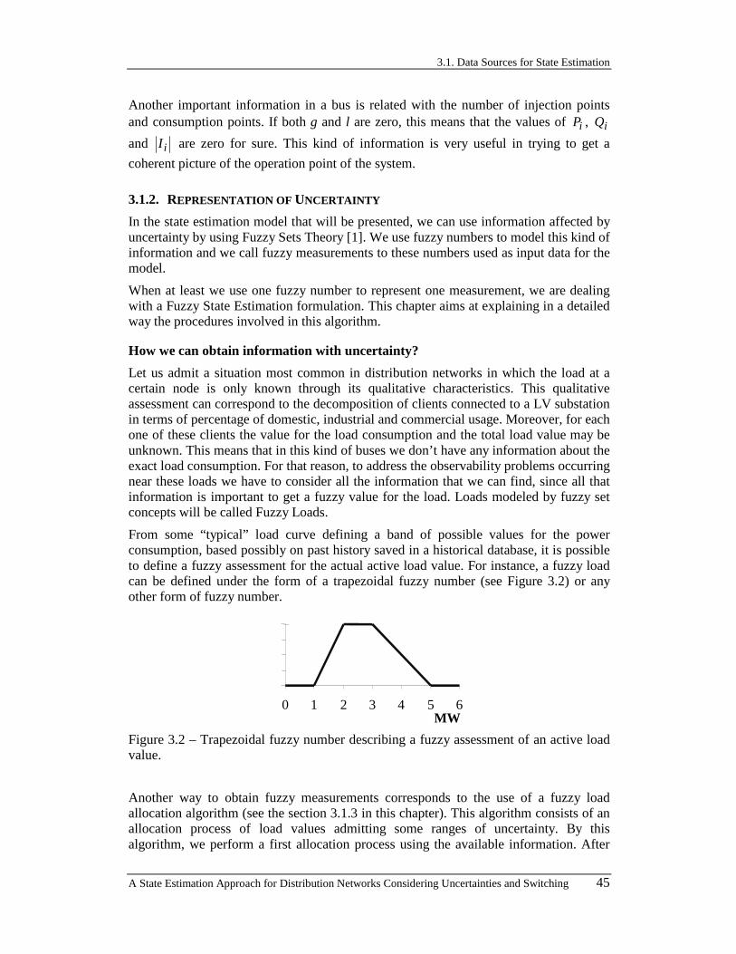
3.1. Data Sources for State Estimation
A State Estimation Approach for Distribution Networks Considering Uncertainties and Switching 45
Another important information in a bus is related with the number of injection points and consumption points. If both g and l are zero, this means that the values of iP , iQ
and iI are zero for sure. This kind of information is very useful in trying to get a
coherent picture of the operation point of the system.
3.1.2. REPRESENTATION OF UNCERTAINTY
In the state estimation model that will be presented, we can use information affected by uncertainty by using Fuzzy Sets Theory [1]. We use fuzzy numbers to model this kind of information and we call fuzzy measurements to these numbers used as input data for the model.
When at least we use one fuzzy number to represent one measurement, we are dealing with a Fuzzy State Estimation formulation. This chapter aims at explaining in a detailed way the procedures involved in this algorithm.
How we can obtain information with uncertainty?
Let us admit a situation most common in distribution networks in which the load at a certain node is only known through its qualitative characteristics. This qualitative assessment can correspond to the decomposition of clients connected to a LV substation in terms of percentage of domestic, industrial and commercial usage. Moreover, for each one of these clients the value for the load consumption and the total load value may be unknown. This means that in this kind of buses we don’t have any information about the exact load consumption. For that reason, to address the observability problems occurring near these loads we have to consider all the information that we can find, since all that information is important to get a fuzzy value for the load. Loads modeled by fuzzy set concepts will be called Fuzzy Loads.
From some “typical” load curve defining a band of possible values for the power consumption, based possibly on past history saved in a historical database, it is possible to define a fuzzy assessment for the actual active load value. For instance, a fuzzy load can be defined under the form of a trapezoidal fuzzy number (see Figure 3.2) or any other form of fuzzy number.
0 1 2 3 4 5 6MW
Figure 3.2 – Trapezoidal fuzzy number describing a fuzzy assessment of an active load value.
Another way to obtain fuzzy measurements corresponds to the use of a fuzzy load allocation algorithm (see the section 3.1.3 in this chapter). This algorithm consists of an allocation process of load values admitting some ranges of uncertainty. By this algorithm, we perform a first allocation process using the available information. After
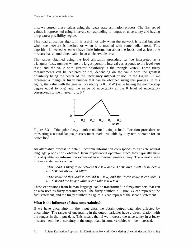
Chapter 3. Fuzzy State Estimation
46 A State Estimation Approach for Distribution Networks Considering Uncertainties and Switching
this, we correct these values using the fuzzy state estimation process. The first set of values is represented using intervals corresponding to ranges of uncertainty and having the greatest possibility degree.
This load allocation algorithm is useful not only when the network is radial but also when the network is meshed or when it is meshed with some radial areas. This algorithm is needed when we have little information about the loads, and at least one measure has an undefined value in an unobservable area.
The values obtained using the load allocation procedure can be interpreted as a triangular fuzzy number where the largest possible interval corresponds to the level zero α-cut and the value with greatest possibility is the triangle vertex. These fuzzy measurements can be centered or not, depending on the value with the greatest possibility being the center of the uncertainty interval or not. In the Figure 3.3 we represent a triangular fuzzy number that can be obtained using this process. In this figure, the value with the greatest possibility is 0.3 MW (value having the membership degree equal to one) and the range of uncertainty at the 0 level of uncertainty corresponds to the interval [0.1, 0.4].
0
1
0 0.1 0.2 0.3 0.4 0.5MW
Figure 3.3 – Triangular fuzzy number obtained using a load allocation procedure or translating a natural language assessment made available by a system operator for an active load.
An alternative process to obtain uncertain information corresponds to translate natural language propositions obtained from experienced operators since they typically have lots of qualitative information expressed in a non-mathematical way. The operator may produce statements such as:
“This load is likely to be between 0.2 MW and 0.3 MW, and it will not be below 0.1 MW nor above 0.4 MW”
“The value of this load is around 0.3 MW, and the lower value it can take is 0.1 MW and the larger value it can take is 0.4 MW”
These expressions from human language can be transformed in fuzzy numbers that can be also used as fuzzy measurements. The fuzzy number in Figure 3.4 can represent the first statement, and the fuzzy number in Figure 3.3 can represent the second statement.
What is the influence of these uncertainties?
If we have uncertainty in the input data, we obtain output data also affected by uncertainty. The ranges of uncertainty in the output variables have a direct relation with the ranges in the input data. This means that if we increase the uncertainty in a fuzzy measurement, the uncertainty in the output data in some variables will be increased.
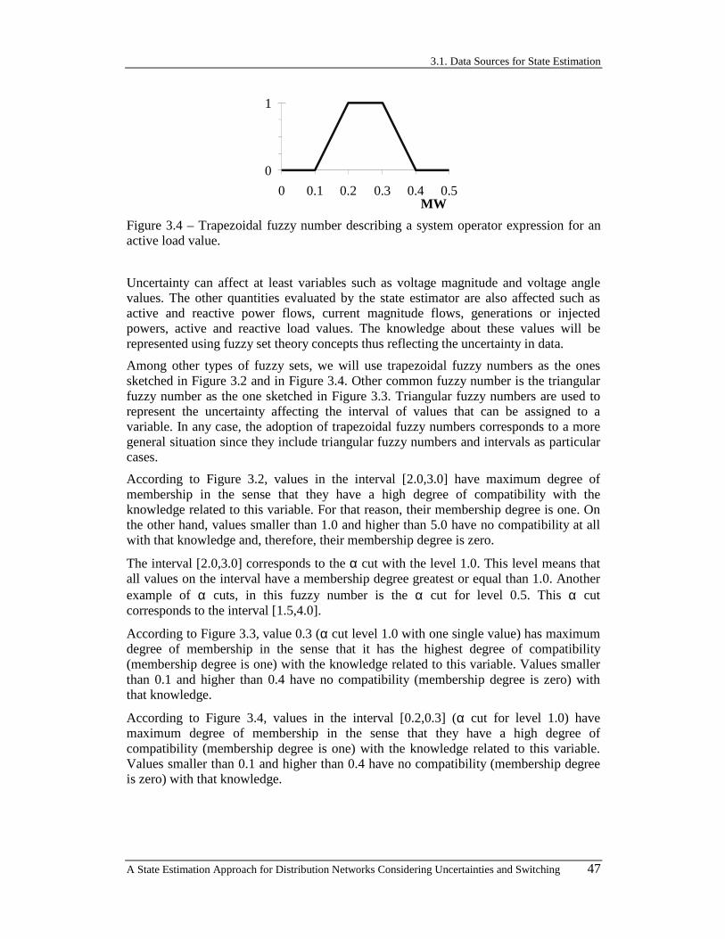
3.1. Data Sources for State Estimation
A State Estimation Approach for Distribution Networks Considering Uncertainties and Switching 47
0
1
0 0.1 0.2 0.3 0.4 0.5MW
Figure 3.4 – Trapezoidal fuzzy number describing a system operator expression for an active load value.
Uncertainty can affect at least variables such as voltage magnitude and voltage angle values. The other quantities evaluated by the state estimator are also affected such as active and reactive power flows, current magnitude flows, generations or injected powers, active and reactive load values. The knowledge about these values will be represented using fuzzy set theory concepts thus reflecting the uncertainty in data.
Among other types of fuzzy sets, we will use trapezoidal fuzzy numbers as the ones sketched in Figure 3.2 and in Figure 3.4. Other common fuzzy number is the triangular fuzzy number as the one sketched in Figure 3.3. Triangular fuzzy numbers are used to represent the uncertainty affecting the interval of values that can be assigned to a variable. In any case, the adoption of trapezoidal fuzzy numbers corresponds to a more general situation since they include triangular fuzzy numbers and intervals as particular cases.
According to Figure 3.2, values in the interval [2.0,3.0] have maximum degree of membership in the sense that they have a high degree of compatibility with the knowledge related to this variable. For that reason, their membership degree is one. On the other hand, values smaller than 1.0 and higher than 5.0 have no compatibility at all with that knowledge and, therefore, their membership degree is zero.
The interval [2.0,3.0] corresponds to the α cut with the level 1.0. This level means that all values on the interval have a membership degree greatest or equal than 1.0. Another example of α cuts, in this fuzzy number is the α cut for level 0.5. This α cut corresponds to the interval [1.5,4.0].
According to Figure 3.3, value 0.3 (α cut level 1.0 with one single value) has maximum degree of membership in the sense that it has the highest degree of compatibility (membership degree is one) with the knowledge related to this variable. Values smaller than 0.1 and higher than 0.4 have no compatibility (membership degree is zero) with that knowledge.
According to Figure 3.4, values in the interval [0.2,0.3] (α cut for level 1.0) have maximum degree of membership in the sense that they have a high degree of compatibility (membership degree is one) with the knowledge related to this variable. Values smaller than 0.1 and higher than 0.4 have no compatibility (membership degree is zero) with that knowledge.

Chapter 3. Fuzzy State Estimation
48 A State Estimation Approach for Distribution Networks Considering Uncertainties and Switching
3.1.3. FUZZY LOAD ALLOCATION
3.1.3.1. The Problem
The problem of generating a coherent load set is critical for distribution networks. This happens because usually the only real time measurements available at a SCADA system installed in a Control Center are the power or current values at the sending end of a feeder coming from a medium voltage (MV) substation. One must therefore rely on other type of data, recorded for instance in commercial files, to try to infer the values of loads.
The need of an inference mechanism resulted in a large research effort in many places. Some models correspond to a more heuristic approach, while others have a probabilistic theoretical background [2]. Some of the primitive approaches to assess line flows in distribution systems addressed the “peak flow” problem: one was only trying to assess the peak flow that could occur at any time in every section of the network.
However, a modern DMS must try to address the problem of evaluating actual synchronized flows and making them compatible with any measurements available at a SCADA system at any time. This is necessary and useful if the DMS is to be used as an effective operation tool. For instance, some switching manoeuvres leading to load transfers may be possible under certain conditions and not technically feasible in other cases.
The complexity of the problem increased with the expanding connection at the distribution level of dispersed generation plants from industrial co-generation, small hydros or wind parks. These connections have two effects:
a) They changed the top-down traditional character of power flows in distribution systems, usually operated under radial configurations. In this case, radial means that there are no loops and that for each sub-network there is only one injection point;
b) In many cases, this power injection is monitored and more real-time measurements are available at the SCADA system, both for power injections and for some line flows.
The model described in [3] derives characteristic load curves for low voltage (LV) substations from commercial data. This model, based on neural networks, was tested and adopted by the Portuguese utility and is giving remarkably accurate results.
However, we can not imagine that all utilities have available, for every LV substation, descriptions of their characteristic daily load curves, for distinct weekdays and seasons of the year. For the LV substations where we have not this information available, neither other type of information, and if we have observability problems near these LV substations, we can run a load allocation algorithm to get a first and rough picture of load values.
3.1.3.2. Algorithm
This section describes a Fuzzy Load Allocation model that was presented in [4], which can be used in a DMS environment. A process of rough allocation is initiated based on information on actual measurements and on data about installed capacity and power and

3.1. Data Sources for State Estimation
A State Estimation Approach for Distribution Networks Considering Uncertainties and Switching 49
energy consumption at LV substations. This process generates a fuzzy load allocation, which is then corrected by a fuzzy state estimation procedure in order to generate a power flow compatible set of load allocations, coherent with available real time measurements recorded in the SCADA.
The loads in a medium voltage (MV) network are mainly composed by low voltage (LV) distribution substations, either public or private. The LV substations can be classified in four general types:
−−−− Type POWER - Substations for which one only knows transformer installed capacity or peak load; capacitors are treated as loads by transforming them into reactive power values under nominal voltage;
−−−− Type ENERGY - Substations for which there is also knowledge about their load composition in terms of three classes of consumers (domestic, industrial and commercial) and their energy consumption for some of them, at peak, normal and valley hours;
−−−− Type CURVE - Substations for which there is also a model, such as described in [3], that allows a prediction of the load at a given hour;
−−−− Type MEASURED - Substations where there are real time power consumption measurements.
The power injection sources in the network are classified in three general types:
−−−− Type ROOT - Main injection point, usually the connection of the substation to a higher voltage level grid;
−−−− Type SOURCE - Any dispersed generation facility for which there are real time measurements in the SCADA system;
−−−− Type NEGATIVE LOAD - Generators for which there are no real time measurements. These are treated as negative loads. Depending on the type of information available, they are merged to one of the previously referred load types.
We assume that there are active and reactive power measurements available for the node ROOT. These values are obtained from the SCADA database or by other information source like the results of a prediction consumption process. If the available measurement corresponds to a current value, a direction and a power factor will be assigned to transform it into active and reactive power values. All other measurements will be considered as corresponding to active or reactive power or voltage. In this model, current measurements will all be transformed into power measurements, but these current values are also used as input data in the state estimation process.
For the algorithm description, we also consider two types of measurements:
−−−− NODAL – measurements at network nodes. Possible points for these type of data are power injection sources type ROOT and type SOURCE, and load nodes;
−−−− BRANCH – measurements obtained from network branches related to lines or transformers.
The basic constraints of the model are:

Chapter 3. Fuzzy State Estimation
50 A State Estimation Approach for Distribution Networks Considering Uncertainties and Switching
−−−− It must represent flows at a given time, in a way they are compatible with the Kirchoff Laws;
−−−− It must display coherency between estimated loads and all available measurements;
−−−− The load allocation must be independent of the network topology under operation.
This last point is important since it would be unacceptable, from an operator point of view, that the estimated load for a given node could change if he performed some switching or load transfer simulation. The traditional concept of “loss of diversity”, when one moves down in a radial network, has no application. In fact, this concept applies to peak values, but it gave place to misconceptions on several occasions.
Besides, the model we will describe does not really require the network topology to be radial: it may be applied to systems with several injection points and to systems with closed loops, with slight adaptations, turning it general.
The model requires the specification of values for two balancing parameters [ ]1;0,m ∈λ . This is a tuning process to be done taking in account the system history and
the operator experience. For instance, if 0=λ , the allocation will be done considering values proportional to the installed capacity or the peak values. Otherwise, if 1=λ , the allocation values will be proportional to average energy consumption values. Another value to be specified is the uncertainty parameter x that may be derived from a linguistic interface about how uncertain an operator feels about estimating loads from the installed capacities.
The model makes an initial rough load allocation for all loads in the network. With these results of this first phase, it is obtained data used as input for the Fuzzy State Estimation model that works like a corrective phase working over the Fuzzy Load Allocation process. To perform a load allocation at instant t, the algorithm includes the following steps:
ROUGH ALLOC
−−−− Discount all MEASURED loads from the ROOT;
−−−− Predict load allocP at every CURVE node and discount it from ROOT. If ROOT power is less than a specified threshold (0, by default), then the CURVE nodes will be treated as ENERGY nodes;
−−−− For CURVE nodes, fix [ ]maxmin P ,P according to (fuzzy) precision indications
associated with the curve models;
−−−− For the nodes in {ENERGY, POWER} calculate, from the installed capacity and peak information, the power powerP , using a balancing parameter
[ ]1;0m ∈ and the expression (3.1);
( ) installedpeakpower mPPm1P +−= (3.1)
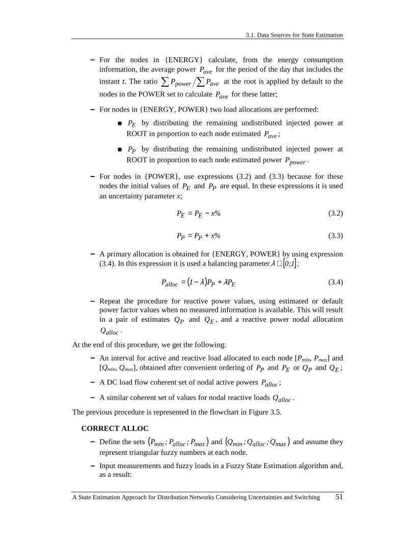
3.1. Data Sources for State Estimation
A State Estimation Approach for Distribution Networks Considering Uncertainties and Switching 51
−−−− For the nodes in {ENERGY} calculate, from the energy consumption information, the average power aveP for the period of the day that includes the
instant t. The ratio ∑∑ avepower PP at the root is applied by default to the
nodes in the POWER set to calculate aveP for these latter;
−−−− For nodes in {ENERGY, POWER} two load allocations are performed:
■ EP by distributing the remaining undistributed injected power at
ROOT in proportion to each node estimated aveP ;
■ PP by distributing the remaining undistributed injected power at
ROOT in proportion to each node estimated power powerP .
−−−− For nodes in {POWER}, use expressions (3.2) and (3.3) because for these nodes the initial values of EP and PP are equal. In these expressions it is used an uncertainty parameter x;
%xPP EE −= (3.2)
%xPP PP += (3.3)
−−−− A primary allocation is obtained for {ENERGY, POWER} by using expression (3.4). In this expression it is used a balancing parameter [ ]1;0∈λ ;
( ) EPalloc PP1P λλ +−= (3.4)
−−−− Repeat the procedure for reactive power values, using estimated or default power factor values when no measured information is available. This will result in a pair of estimates PQ and EQ , and a reactive power nodal allocation
allocQ .
At the end of this procedure, we get the following:
−−−− An interval for active and reactive load allocated to each node [Pmin, Pmax] and [Qmin, Qmax], obtained after convenient ordering of PP and EP or PQ and EQ ;
−−−− A DC load flow coherent set of nodal active powers allocP ;
−−−− A similar coherent set of values for nodal reactive loads allocQ .
The previous procedure is represented in the flowchart in Figure 3.5.
CORRECT ALLOC
−−−− Define the sets ( )maxallocmin P ;P ;P and ( )maxallocmin Q ;Q ;Q and assume they represent triangular fuzzy numbers at each node.
−−−− Input measurements and fuzzy loads in a Fuzzy State Estimation algorithm and, as a result:

Chapter 3. Fuzzy State Estimation
52 A State Estimation Approach for Distribution Networks Considering Uncertainties and Switching
■ Define, for each load, the final allocP and allocQ ;
■ Define, for each branch, a credible flow F and lower and upper bound flows [ ]maxmin F;F .
−−−− Compare branch flow limit itlimF with minF , F and maxF and activate, if necessary, a level of alarm.
At the end of this procedure, the allocP and allocQ values plus the measurements form an AC Power Flow coherent set of values.
Pi,E = PROOT ×××× Pi,ave/ PSUM,avePi,P = PROOT ×××× Pi,power / PSUM,power
for each node i of type MEASUREDPROOT = PROOT - Pi
begin
for each node i of type CURVEpredict Pi , Pi,min , Pi,max
PROOT = PROOT - Pi
PROOT < 0for each node i of type CURVEchange node i type to ENERGY
yes
for each node i of type ENERGYcalculate Pi,ave in this period
Pi,power = (1-m)××××Pi,peak + m××××Pi,installed
PROOT,ratio = ΣΣΣΣPi,power / ΣΣΣΣ Pi,ave
no
for each node i of type POWERPi,power = (1-m)××××Pi,peak + m××××Pi,installed
Pi,ave = Pi,power / PROOT,ratio
Pi,E = Pi,PPi,E= Pi,E -x%Pi,P= Pi,P +x%
yes
no
Pi = (1-λλλλ)××××Pi,P + λ×λ×λ×λ×Pi,E
end
for each node i oftype POWER or
ENERGY
Figure 3.5 – Flowchart for the rough load allocation algorithm of the active power.

3.1. Data Sources for State Estimation
A State Estimation Approach for Distribution Networks Considering Uncertainties and Switching 53
3.1.3.3. Example
The Fuzzy State Estimation algorithm used as the CORRECT ALLOC procedure will be presented in the following sections of this Chapter and will be illustrated using a larger network in Chapter 7. At this moment, we selected a small scale illustrative example, that is a part of the network used in Chapter 7, in order to detail the application of the Fuzzy Load Allocation procedure. This illustrative network has 14 buses and it is represented in Figure 3.6.
25
27
30
34
35
2826
36 38
31
37
29
32
33
61.09 MW12.82 Mvar
54.79 MW11.75 Mvar
64.49 MW13.87 Mvar
Figure 3.6 – Network example for the application of the described fuzzy load allocation algorithm.
Figure 3.6 represents a system for which we admitted the existence of active and reactive power flow measurements on all lines that leave the substation connected to bus 25. In the LV substations, it is possible to run a procedure of rough load allocation and we can consider that the general type of these buses, based in the information available, is ENERGY type. The parameters needed to run the load allocation procedure are indicated in Table 3.1. The balancing parameter m is assigned the value 0.5, the uncertainty parameter x has the value 5% and the balancing parameter λ has the value 0.5.
Using these parameters and the available measurements of type BRANCH it is possible to run the ROUGH ALLOC procedure described in the previous section. This procedure will be run considering a sub-network formed by buses 25, 26, 29, 32 and 33 that have the ROOT in the branch from bus 25 to bus 26. This ROOT has a measure with value 61.09 MW for the active power flow and 12.82 Mvar for the reactive power flow. Another sub-network is formed by buses 25, 27, 30, 34 and 35 and have the ROOT in the branch from 25 to bus 27. This ROOT has a measure with the value 64.49 MW for the active power flow and 13.87 Mvar for the reactive power flow. Finally, the third sub-network is formed by buses 25, 28, 31, 36, 37 and 38 and has the ROOT in the branch from bus 25 to bus 28. This ROOT has a measure with value 54.79 MW for the active power flow and 11.75 Mvar for the reactive power flow.
After running the referred algorithm in each sub-network we obtain the sets of values ( )maxallocmin P ;P ;P and ( )maxallocmin Q ;Q ;Q that will be used as input of the Fuzzy

Chapter 3. Fuzzy State Estimation
54 A State Estimation Approach for Distribution Networks Considering Uncertainties and Switching
State Estimation algorithm. These values are used as fuzzy measurements having triangular membership functions. In this case, the values obtained are indicated in Table 3.2.
Bus# peakP
(MW) installedP (MW)
aveP
(MW) peakQ
(Mvar) installedQ (Mvar)
aveQ
(Mvar)
26 50.00 75.00 28.25 12.75 20.40 6.67 27 50.00 75.00 27.00 10.20 16.30 5.60 28 50.00 80.00 27.00 10.20 16.30 5.60 29 30.00 45.00 13.75 7.75 10.90 3.25 30 30.00 45.00 13.00 6.20 8.70 2.60 31 30.00 42.00 13.00 6.20 8.70 2.60 32 20.00 30.00 9.50 5.25 7.90 3.04 33 20.00 30.00 11.50 5.25 7.90 3.04 34 20.00 30.00 9.00 4.20 6.30 2.60 35 10.00 15.00 6.00 1.90 2.90 1.45 36 20.00 30.00 9.00 4.20 6.30 2.60 37 20.00 30.00 11.00 4.20 6.30 2.60 38 10.00 15.00 5.00 1.90 2.90 0.95
Table 3.1 – Values for the parameters used to run the rough load allocation algorithm for all the LV substations of ENERGY type.
Bus# minP
(MW) allocP
(MW) maxP
(MW) minQ
(Mvar) allocQ
(Mvar) maxQ
(Mvar)
26 -27.39 -26.42 -25.45 -5.44 -5.39 -5.34 27 -26.90 -25.90 -24.91 -5.49 -5.43 -5.37 28 -26.79 -26.21 -25.64 -5.47 -5.44 -5.41 29 -15.27 -14.30 -13.33 -3.06 -2.83 -2.60 30 -14.94 -13.95 -12.95 -3.09 -2.79 -2.49 31 -14.20 -13.55 -12.90 -3.08 -2.79 -2.51 32 -10.18 -9.70 -9.21 -2.44 -2.30 -2.16 33 -11.15 -10.67 -10.18 -2.44 -2.30 -2.16 34 -9.96 -9.46 -8.97 -2.49 -2.34 -2.18 35 -5.98 -5.48 -4.98 -1.39 -1.19 -1.00 36 -9.86 -9.40 -8.93 -2.51 -2.34 -2.17 37 -10.91 -10.39 -9.86 -2.51 -2.34 -2.17 38 -4.96 -4.95 -4.93 -0.99 -0.95 -0.92
Table 3.2 – Values obtained from the rough load allocation algorithm for all the LV substations.
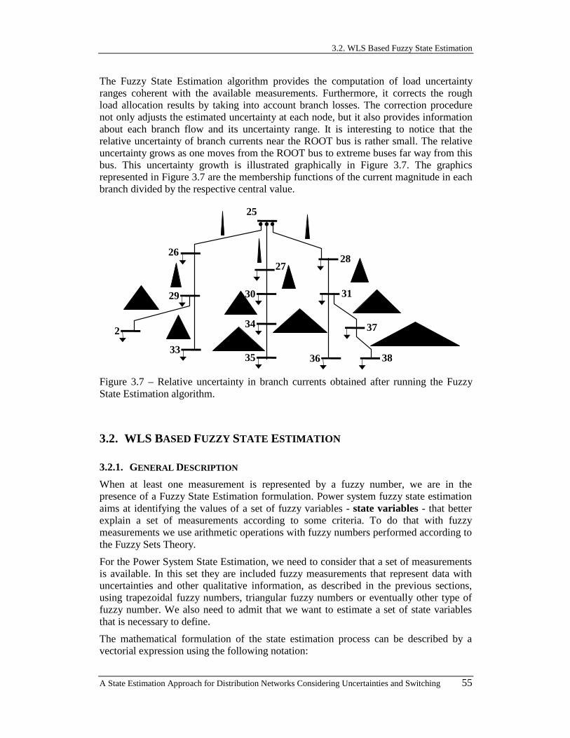
3.2. WLS Based Fuzzy State Estimation
A State Estimation Approach for Distribution Networks Considering Uncertainties and Switching 55
The Fuzzy State Estimation algorithm provides the computation of load uncertainty ranges coherent with the available measurements. Furthermore, it corrects the rough load allocation results by taking into account branch losses. The correction procedure not only adjusts the estimated uncertainty at each node, but it also provides information about each branch flow and its uncertainty range. It is interesting to notice that the relative uncertainty of branch currents near the ROOT bus is rather small. The relative uncertainty grows as one moves from the ROOT bus to extreme buses far way from this bus. This uncertainty growth is illustrated graphically in Figure 3.7. The graphics represented in Figure 3.7 are the membership functions of the current magnitude in each branch divided by the respective central value.
25
27
30
34
35
2826
36 38
31
37
29
2
33
Figure 3.7 – Relative uncertainty in branch currents obtained after running the Fuzzy State Estimation algorithm.
3.2. WLS BASED FUZZY STATE ESTIMATION
3.2.1. GENERAL DESCRIPTION
When at least one measurement is represented by a fuzzy number, we are in the presence of a Fuzzy State Estimation formulation. Power system fuzzy state estimation aims at identifying the values of a set of fuzzy variables - state variables - that better explain a set of measurements according to some criteria. To do that with fuzzy measurements we use arithmetic operations with fuzzy numbers performed according to the Fuzzy Sets Theory.
For the Power System State Estimation, we need to consider that a set of measurements is available. In this set they are included fuzzy measurements that represent data with uncertainties and other qualitative information, as described in the previous sections, using trapezoidal fuzzy numbers, triangular fuzzy numbers or eventually other type of fuzzy number. We also need to admit that we want to estimate a set of state variables that is necessary to define.
The mathematical formulation of the state estimation process can be described by a vectorial expression using the following notation:
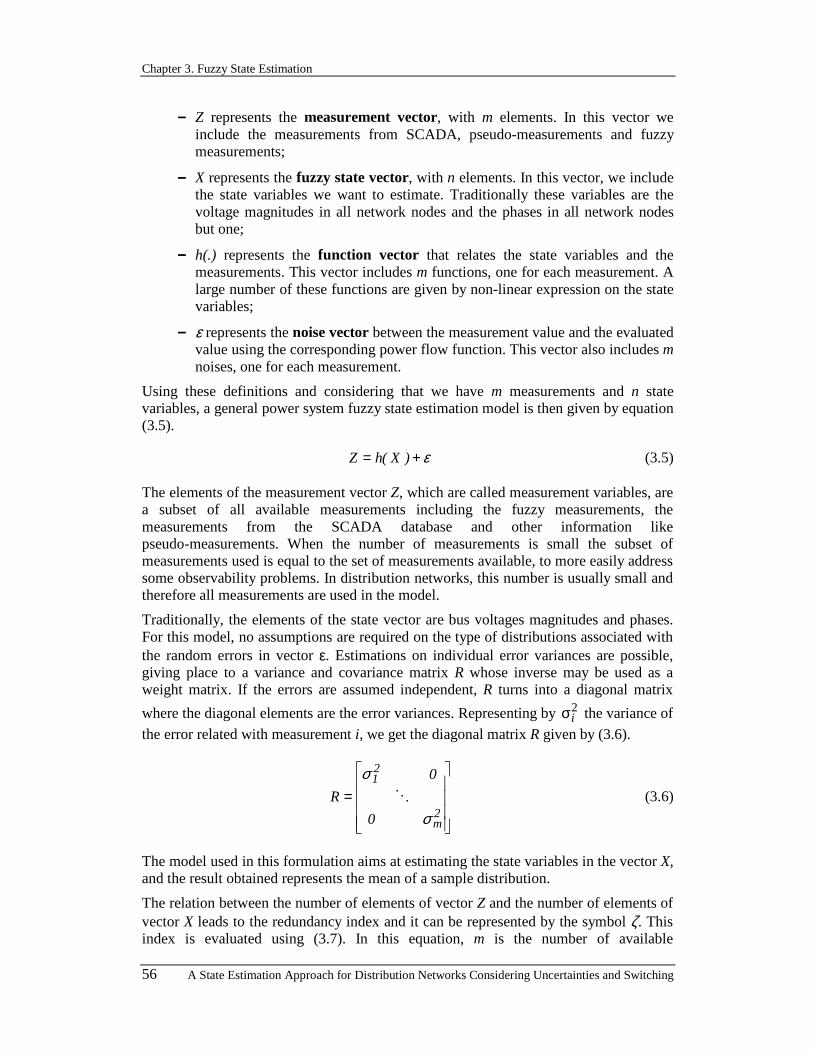
Chapter 3. Fuzzy State Estimation
56 A State Estimation Approach for Distribution Networks Considering Uncertainties and Switching
−−−− Z represents the measurement vector, with m elements. In this vector we include the measurements from SCADA, pseudo-measurements and fuzzy measurements;
−−−− X represents the fuzzy state vector, with n elements. In this vector, we include the state variables we want to estimate. Traditionally these variables are the voltage magnitudes in all network nodes and the phases in all network nodes but one;
−−−− h(.) represents the function vector that relates the state variables and the measurements. This vector includes m functions, one for each measurement. A large number of these functions are given by non-linear expression on the state variables;
−−−− ε represents the noise vector between the measurement value and the evaluated value using the corresponding power flow function. This vector also includes m noises, one for each measurement.
Using these definitions and considering that we have m measurements and n state variables, a general power system fuzzy state estimation model is then given by equation (3.5).
ε+= )X(hZ (3.5)
The elements of the measurement vector Z, which are called measurement variables, are a subset of all available measurements including the fuzzy measurements, the measurements from the SCADA database and other information like pseudo-measurements. When the number of measurements is small the subset of measurements used is equal to the set of measurements available, to more easily address some observability problems. In distribution networks, this number is usually small and therefore all measurements are used in the model.
Traditionally, the elements of the state vector are bus voltages magnitudes and phases. For this model, no assumptions are required on the type of distributions associated with the random errors in vector ε. Estimations on individual error variances are possible, giving place to a variance and covariance matrix R whose inverse may be used as a weight matrix. If the errors are assumed independent, R turns into a diagonal matrix
where the diagonal elements are the error variances. Representing by 2iσ the variance of
the error related with measurement i, we get the diagonal matrix R given by (3.6).
=2m
21
0
0
R
σ
σO (3.6)
The model used in this formulation aims at estimating the state variables in the vector X, and the result obtained represents the mean of a sample distribution.
The relation between the number of elements of vector Z and the number of elements of vector X leads to the redundancy index and it can be represented by the symbol ζ. This index is evaluated using (3.7). In this equation, m is the number of available

3.2. WLS Based Fuzzy State Estimation
A State Estimation Approach for Distribution Networks Considering Uncertainties and Switching 57
measurements (elements of vector Z) and n is the number of state variables (elements of vector X).
n
m=ζ (3.7)
The redundancy index must have a value larger than 1.0, otherwise the network is not observable. If this value is larger than 1.0 the network can still be not observable. Furthermore, it is also needed that the available measurements are distributed uniformly in the entire network and that it will be possible to evaluate each state variable for each node using the available information.
3.2.2. ALGORITHM TO COMPUTE STATE VARIABLES
The problem of power system state estimation can be solved using an algorithm that aims at identifying the values of the state variables that minimize the weighted sum of the square errors, according to expression (3.8). This kind of algorithm is called Weighted Least Squares (WLS) and corresponds to the most well known and widely used and described one.
εε 1T −Rmin (3.8)
The weights may correspond to the inverse of the measurement variances, contributing to give more credibility to the measurements from more precise devices. Apart from this, flexible procedures for the weight allocation may be adopted to represent several other characteristics of the real world problem. Besides this, it is also necessary to define weights for the other information not coming from the SCADA database but have another source. When other equations are inserted in the model (3.5) to represent some knowledge about state variables, it is also needed to define weights for the corresponding measurements.
[ ] [ ])X(hZR)X(hZ 1T −− −min (3.9)
Expression (3.8) represents a Weighted Least Square problem whose solution algorithm is well known. Expression (3.9) is obtained by replacing ε in this expression by an expression obtained from (3.5). This minimization problem is solved by formulating a set of equations expressing the stationary conditions of this function, called normal equations.
The function to be minimized in (3.9) can be rewritten in terms of the performance index ( )XJ given by (3.10). The above referred normal equations are obtained by
getting the derivatives of ( )XJ regarding the state variables X and putting them equal to zero thus leading to (3.11).
( )
XhZ
2
1J(X)
m
1j
2
j
jj∑=
−=
σ (3.10)

Chapter 3. Fuzzy State Estimation
58 A State Estimation Approach for Distribution Networks Considering Uncertainties and Switching
( )0.0
X
(X)h
XhZ
X
J(X) jm
1j j
jj =∂
∂
−−=
∂∂ ∑
= σ (3.11)
Finally, we obtain the normal equations given by expression (3.12) using matrix notation. In this expression H(X) represents the measurement Jacobian matrix, which is evaluated using the derivatives represented in (3.13).
[ ] 0)X(hZR)X(H 1T =−− (3.12)
( ) ( )
( ) ( )
∂∂
∂∂
∂∂
∂∂
=
n
m
1
m
n
1
1
1
X
Xh
X
Xh
X
Xh
X
Xh
)X(H
L
MOM
L
(3.13)
The computation of the state vector corresponding to the measurement vector Z is performed by solving the set of non-linear equations (3.12). This set of equations can be solved by an iterative process using the Newton-Raphson´s method. At the (k+1)th iteration the refreshed values of the state variables can be obtained from the values in the iteration k by (3.14). In this equation G is the gain matrix given by (3.15).
( )[ ] ( )[ ]
−+= −− k1Tk1kk1k+ XhZRXHXGXX (3.14)
( ) ( )[ ] ( )k1Tkk XHRXHXG −= (3.15)
This algorithm evaluates the state variables if the measurements are enough to deal with the observability problem, and if there are no fuzzy measurements. With fuzzy measurements this algorithm needs some simplifications in order to turn it computationally possible and, by this way, finding the fuzzy state variables. If we try to apply fuzzy operations directly to the equations (3.14) and (3.15) we would need a long period of time to do these operations and the uncertainty in the results would be so large that the results would be of little significance.
Let us consider that we have a fuzzy vector of measurements FZ . This means that this vector integrates, at least, one measurement modeled by a fuzzy number. This fuzzy vector can be decomposed in a crisp vector of measurements Z and in a fuzzy vector of deviations FZ∆ . The vector Z can be obtained from FZ by replacing each fuzzy
measurement in FZ by its Central Value while the vector of deviations FZ∆ can be
obtained by performing the subtraction between FZ and Z using the rules of fuzzy arithmetic (see equation (3.16)). An important detail is that each element of the vector of deviations FZ∆ has a Central Value equal to zero.
FF ZZZ ∆+= (3.16)
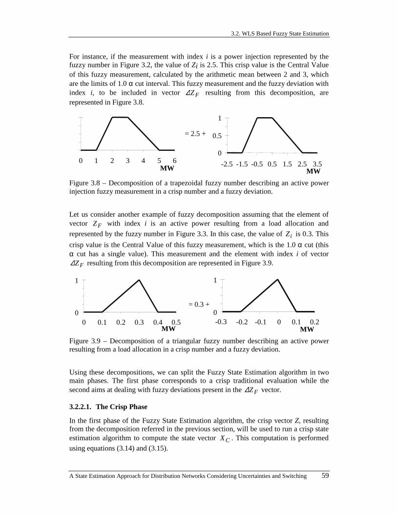
3.2. WLS Based Fuzzy State Estimation
A State Estimation Approach for Distribution Networks Considering Uncertainties and Switching 59
For instance, if the measurement with index i is a power injection represented by the fuzzy number in Figure 3.2, the value of Zi is 2.5. This crisp value is the Central Value of this fuzzy measurement, calculated by the arithmetic mean between 2 and 3, which are the limits of 1.0 α cut interval. This fuzzy measurement and the fuzzy deviation with index i, to be included in vector FZ∆ resulting from this decomposition, are represented in Figure 3.8.
0 1 2 3 4 5 6MW
= 2.5 +
0
0.5
1
-2.5 -1.5 -0.5 0.5 1.5 2.5 3.5MW
Figure 3.8 – Decomposition of a trapezoidal fuzzy number describing an active power injection fuzzy measurement in a crisp number and a fuzzy deviation.
Let us consider another example of fuzzy decomposition assuming that the element of vector FZ with index i is an active power resulting from a load allocation and
represented by the fuzzy number in Figure 3.3. In this case, the value of iZ is 0.3. This
crisp value is the Central Value of this fuzzy measurement, which is the 1.0 α cut (this α cut has a single value). This measurement and the element with index i of vector
FZ∆ resulting from this decomposition are represented in Figure 3.9.
0
1
0 0.1 0.2 0.3 0.4 0.5MW
= 0.3 + 0
1
-0.3 -0.2 -0.1 0 0.1 0.2MW
Figure 3.9 – Decomposition of a triangular fuzzy number describing an active power resulting from a load allocation in a crisp number and a fuzzy deviation.
Using these decompositions, we can split the Fuzzy State Estimation algorithm in two main phases. The first phase corresponds to a crisp traditional evaluation while the second aims at dealing with fuzzy deviations present in the FZ∆ vector.
3.2.2.1. The Crisp Phase
In the first phase of the Fuzzy State Estimation algorithm, the crisp vector Z, resulting from the decomposition referred in the previous section, will be used to run a crisp state estimation algorithm to compute the state vector CX . This computation is performed
using equations (3.14) and (3.15).

Chapter 3. Fuzzy State Estimation
60 A State Estimation Approach for Distribution Networks Considering Uncertainties and Switching
In this phase, the elements of the noise vector associated to the fuzzy measurements are considered to be independent and have zero means. The zero value for the mean of a fuzzy noise can be interpreted, in fact, as the mean of all central values considering the fuzzy representation of the noises of those measurements. Therefore, these elements of the noise vector have a fuzzy mean with central value equal to zero.
The fuzzy representation of noises is needed because if in the equation model (3.5) are included fuzzy measurements it is also necessary to include fuzzy noises (see Figure 3.10).
0
1
0.8 0.9 1 1.1 1.2
Zi (p.u.)
=
0
1
0.8 0.9 1 1.1 1.2
hi(X)
+
0
1
-0.15 -0.05 0.05
εi
Figure 3.10 – Three fuzzy numbers representing one possible equation of the general fuzzy state estimation model given by (3.5).
At this point, it should be stressed that all measurement errors are represented by a probability distribution although the mean values of some of them (the fuzzy measurements) are affected by uncertainty represented by fuzzy numbers. This means that noises related to the fuzzy measurements are considered to have a probability distribution with a fuzzy mean, corresponding to a value around zero.
3.2.2.2. The Fuzzy Phase
In the second phase of the Fuzzy State Estimation algorithm, the fuzzy deviations specified for the measurements are reflected on the results of the state estimation. These results are obtained using the state vector CX , the gain matrix inverse G-1 and the
Jacobian matrix H computed in the last iteration of the previously run crisp state estimation (the first phase of this algorithm). Therefore, estimates of the variations for the fuzzy state variables can be obtained using equation (3.17).
[ ] ( )[ ]C1T1 XhZRHGX −×=∆ −−
(3.17)
How can we obtain this equation?
In Figure 3.11 it is represented graphically the iterative Newton-Raphson algorithm, used in the first phase, for two consecutive iterations considering an unidimensional case, only for representation purposes. As we see, at each iteration of this algorithm it is performed a linearization of the function ( )Xf . The linearization in the k iteration is
done considering the derivative ( )kXf ′ of the function ( )Xf around the current point kX , and the next point 1kX + is evaluated using this simplification (see equation
(3.18), which in fact is in line with equation (3.14)).

3.2. WLS Based Fuzzy State Estimation
A State Estimation Approach for Distribution Networks Considering Uncertainties and Switching 61
( )[ ] ( )k1kk1k XfX'fXX−+ −= (3.18)
Xk
f(X)
linearization of f(X)in iteration k
Xk+1
f(Xk)
f(Xk+1)
Xk+2
f(Xk+2)[ ])X(hZR)X(H)X(f 1T −= −
where
X
Figure 3.11 – Graphical representation of the Newton-Raphson’s algorithm to obtain the solution of an equation as ( ) 0Xf = .
Using the linearization done in the last iteration of Newton-Raphson´s algorithm, we can easily evaluate an approximation for the deviations of the function ( )Xf given some deviations on the input variable X . In the same way, we can also evaluate an approximation for the deviations on the variable X for some deviations on the function
( )Xf . In the point CX obtained in the last iteration of the iterative process, the value of the function in this point is approximately zero. In our function, this means that Z is approximately equal to ( )CXh and a small deviation in the value of Z corresponds to a
small deviation in the value of function ( )Xf .
In the Figure 3.12 it is represented for an unidimensional case, the result obtained using this linearization and the exact value (deviation of 2d in the value of CX ) for a
deviation 1d in the function value ( )CXf . The point CX is the result of the iterative process and also corresponds to the point where the linearization is performed when starting the fuzzy phase.
According to expression (3.17), we evaluate the fuzzy deviation of a measurement by the difference between each fuzzy measurement in Z and the crisp value obtained for that measurement by the corresponding ( )Xh function evaluated using the crisp state
variables in CX . This is a fuzzy vector because some elements of vector Z are fuzzy
numbers, and will now be multiplied by the matrix 11 −− RHG T . This matrix is obtained in the last iteration in the crisp phase. To do this operation, we use fuzzy arithmetic rules in order to compute the fuzzy vector ∆X that correspond to the fuzzy deviations affecting the state variables.

Chapter 3. Fuzzy State Estimation
62 A State Estimation Approach for Distribution Networks Considering Uncertainties and Switching
f(X)linearization of f(X)in the last iteration
XC
f(XC)+d1
f(XC)[ ])X(hZR)X(H)X(f
where
C1T
CC −= −
XC+d2
exact value
X
Figure 3.12 – Representation of the result deviation (exact value and an approximation) for a deviation in the value of the function.
XXX CF ∆+= (3.19)
According to expression (3.19), the final fuzzy state vector FX is obtained by
performing the fuzzy addition of the fuzzy vector X∆ with the crisp state vector CX
computed in the first phase of the algorithm. An important point to consider regarding these calculations is that the fuzzy state vector is computed directly from fuzzy deviations in the measures. In this way, we can determine the influence of measurement uncertainties in some elements in the results. These influences are computed using the
elements of 11 −− RHG T matrix and with some arithmetic operations easily performed.
With the described algorithm, one is able to characterize the state estimation results in terms of membership functions for the state variables. These variables have a probabilistic nature since in traditional state estimation models the error measurements are assigned a probabilistic interpretation. However, they also have a fuzzy nature since we considered that error means are represented by fuzzy numbers having a zero central value. Accordingly, this Fuzzy State Estimation model represents a novel and hybrid way of combining two theoretical frameworks to model uncertainty: probabilistic and fuzzy models. Fuzzy Sets and Probabilities are not competing against each other, instead they must be seen as complementary and used whenever they are more adequate.
3.2.3. COMPUTATION OF OTHER VARIABLES
System operators in control centers can also be interested in analyzing the possible behavior of other variables, such as:
−−−− Active and reactive power flows;
−−−− Currents in lines and transformers;
−−−− Power injected by generators or by connections with other networks;

3.2. WLS Based Fuzzy State Estimation
A State Estimation Approach for Distribution Networks Considering Uncertainties and Switching 63
−−−− Active and reactive load values.
However, the evaluation of the membership functions of these variables should not be performed using the fuzzy values of the state variables computed with the previous algorithm. The required arithmetic operations are possible, but the results should display too large uncertainties due to the large number of arithmetic operations to be performed.
These membership functions can be obtained directly from the values of the original fuzzy measurements. To do this we can linearize a generic function ijF , representing
either branch active and reactive power flows or currents. Taking the first terms of its Taylor's series computed around CX , represented in expression (3.20), we obtain expression (3.21). In expression (3.21) it is considered that a deviation in a power flow or current is approximated by a linear expression depending on voltages and phases deviations on the extremes buses.
( ) ( ) ( )
( )444 3444 21
Cj
ii
i
CijCijCij
XiF
XX
XFXFXXF
∆
∆∆ ∑
∂∂
+≅+
(3.20)
( ) ( ) ( ) ( ) ( )j
j
Ciji
i
Cijj
j
Ciji
i
CijCij V
V
XFV
V
XFXFXFXF ∆
∂∂
∆∂
∂θ∆
∂θ∂
θ∆∂θ
∂∆ +++≅ (3.21)
In expression (3.21) we have the following variables:
−−−− ijF represents a generic function representing a branch flow in the line between
buses i and j;
−−−− CX represents the crisp state vector resulting from the first phase of the
algorithm as described in section 3.2.2.1 (page 59);
−−−− iV and jV represent the voltage magnitudes in buses i and j respectively,
corresponding to elements of the state vector X;
−−−− iθ and jθ represent the voltage angles in buses i and j respectively
corresponding to elements of the state vector X.
The derivatives of ijF in expression (3.21) can be organized in one matrix represented
by ( )CF XJ and with a form similar to the one represented in (3.22). Each element of
this matrix corresponds to the derivatives of each flow regarding the elements of the state vector CX . In this matrix representation, the elements in (3.22) for the line related
with the function ijF are the only ones that are different from zero, all the other
elements in that line are zero.
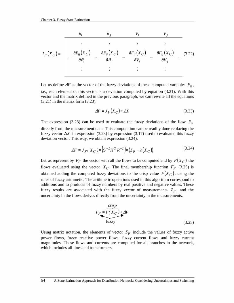
Chapter 3. Fuzzy State Estimation
64 A State Estimation Approach for Distribution Networks Considering Uncertainties and Switching
( ) ( ) ( ) ( ) ( )
MMMM
MMMM
...j
Cij...
i
Cij...
j
Cij...
i
Cij...
j iji
CF
V
XF
V
XFXFXF
VV
XJ
∂
∂
∂
∂
∂
∂
∂
∂=θθ
θθ
(3.22)
Let us define ∆F as the vector of the fuzzy deviations of these computed variables ijF ,
i.e., each element of this vector is a deviation computed by equation (3.21). With this vector and the matrix defined in the previous paragraph, we can rewrite all the equations (3.21) in the matrix form (3.23).
( ) XXJF CF ∆∆ ×= (3.23)
The expression (3.23) can be used to evaluate the fuzzy deviations of the flow ijF
directly from the measurement data. This computation can be readily done replacing the fuzzy vector X∆ in expression (3.23) by expression (3.17) used to evaluated this fuzzy deviation vector. This way, we obtain expression (3.24).
( ) ( )( )CF1T1
CF XhZRHG)X(JF −××= −−∆ (3.24)
Let us represent by FF the vector with all the flows to be computed and by ( )CXF the
flows evaluated using the vector CX . The final membership function FF (3.25) is
obtained adding the computed fuzzy deviations to the crisp value ( )CXF , using the
rules of fuzzy arithmetic. The arithmetic operations used in this algorithm correspond to additions and to products of fuzzy numbers by real positive and negative values. These fuzzy results are associated with the fuzzy vector of measurements FZ , and the uncertainty in the flows derives directly from the uncertainty in the measurements.
fuzzy
F
crisp
)X(FF CF ∆+=48476
(3.25)
Using matrix notation, the elements of vector FF include the values of fuzzy active power flows, fuzzy reactive power flows, fuzzy current flows and fuzzy current magnitudes. These flows and currents are computed for all branches in the network, which includes all lines and transformers.

3.2. WLS Based Fuzzy State Estimation
A State Estimation Approach for Distribution Networks Considering Uncertainties and Switching 65
3.2.3.1. Power Flows
Let us now consider the line between bus i and bus j, represented in Figure 3.13. When the flow we want to compute is an active or a reactive power flow in this line the corresponding elements in vector FF are represented by:
−−−− Pij to represent the active power flow;
−−−− Qij to represent the reactive power flow.
bus i bus j
shij
shij jby = sh
jishji jby =
ijijij jbgy +=
ijijij jQPS += jijiji jQPS +=
Figure 3.13 – Representation of π equivalent model of a line between buses i and j.
The formulas used to evaluate these values based on the crisp state vector CX are given
by expression (3.26) for the active power flow (denoted by ( )Cij XP ) and by expression
(3.27) for the reactive power flow (denoted by ( )Cij XQ ).
( ) ( ) ( )( )jiijjiijji2
iijCij sinbcosgVVVgXP θθθθ −+−−= (3.26)
( ) ( ) ( ) ( )( )jiijjiijji2
ishijijCij singcosbVVVbbXQ θθθθ −−−++−= (3.27)
In these expressions and also in Figure 3.13, we use the following notation:
−−−− iV and jV represent the voltage magnitudes in buses i and j respectively. These
variables are elements of vector CX ;
−−−− iθ and jθ represent the voltage angles in buses i and j respectively. These
variables are elements of vector CX ;
−−−− ijy represents the line admittance, corresponding to a complex value;
−−−− ijg represents the line conductance, that is the real part of the line admittance;
−−−− ijb represents the line susceptance, that is the imaginary part of the line
admittance;
−−−− shijy and sh
jiy represent the line shunt admittances in the extremities i and j
respectively;
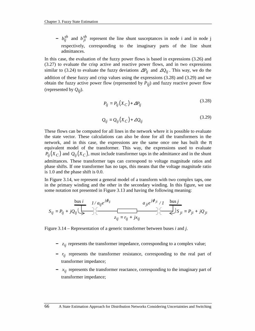
Chapter 3. Fuzzy State Estimation
66 A State Estimation Approach for Distribution Networks Considering Uncertainties and Switching
−−−− shijb and sh
jib represent the line shunt susceptances in node i and in node j
respectively, corresponding to the imaginary parts of the line shunt admittances.
In this case, the evaluation of the fuzzy power flows is based in expressions (3.26) and (3.27) to evaluate the crisp active and reactive power flows, and in two expressions similar to (3.24) to evaluate the fuzzy deviations ijP∆ and ijQ∆ . This way, we do the
addition of these fuzzy and crisp values using the expressions (3.28) and (3.29) and we obtain the fuzzy active power flow (represented by Pij) and fuzzy reactive power flow (represented by Qij).
( ) ijCijij PXPP ∆+= (3.28)
( ) ijCijij QXQQ ∆+= (3.29)
These flows can be computed for all lines in the network where it is possible to evaluate the state vector. These calculations can also be done for all the transformers in the network, and in this case, the expressions are the same once one has built the π equivalent model of the transformer. This way, the expressions used to evaluate
( )Cij XP and ( )Cij XQ , must include transformer taps in the admittance and in the shunt
admittances. These transformer taps can correspond to voltage magnitude ratios and phase shifts. If one transformer has no taps, this means that the voltage magnitude ratio is 1.0 and the phase shift is 0.0.
In Figure 3.14, we represent a general model of a transform with two complex taps, one in the primary winding and the other in the secondary winding. In this figure, we use some notation not presented in Figure 3.13 and having the following meaning:
bus i bus jijjijea/1
ϕ
ijijij jxrz +=ijijij jQPS += jijiji jQPS +=
1/ea jijji
ϕ
Figure 3.14 – Representation of a generic transformer between buses i and j.
−−−− ijz represents the transformer impedance, corresponding to a complex value;
−−−− ijr represents the transformer resistance, corresponding to the real part of
transformer impedance;
−−−− ijx represents the transformer reactance, corresponding to the imaginary part of
transformer impedance;
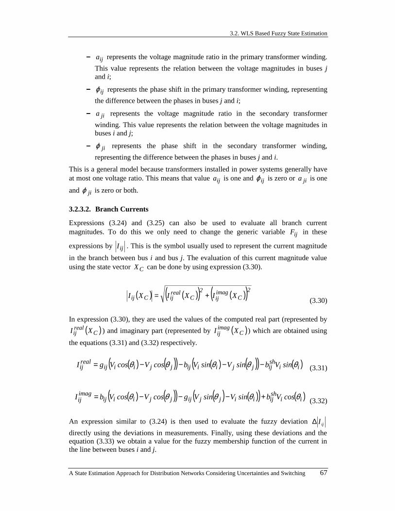
3.2. WLS Based Fuzzy State Estimation
A State Estimation Approach for Distribution Networks Considering Uncertainties and Switching 67
−−−− ija represents the voltage magnitude ratio in the primary transformer winding.
This value represents the relation between the voltage magnitudes in buses j and i;
−−−− ijϕ represents the phase shift in the primary transformer winding, representing
the difference between the phases in buses j and i;
−−−− jia represents the voltage magnitude ratio in the secondary transformer
winding. This value represents the relation between the voltage magnitudes in buses i and j;
−−−− jiϕ represents the phase shift in the secondary transformer winding,
representing the difference between the phases in buses j and i.
This is a general model because transformers installed in power systems generally have at most one voltage ratio. This means that value ija is one and ijϕ is zero or jia is one
and jiϕ is zero or both.
3.2.3.2. Branch Currents
Expressions (3.24) and (3.25) can also be used to evaluate all branch current magnitudes. To do this we only need to change the generic variable ijF in these
expressions by ijI . This is the symbol usually used to represent the current magnitude
in the branch between bus i and bus j. The evaluation of this current magnitude value using the state vector CX can be done by using expression (3.30).
( ) ( )( ) ( )( )2Cimagij
2C
realijCij XIXIXI +=
(3.30)
In expression (3.30), they are used the values of the computed real part (represented by
( )Crealij XI ) and imaginary part (represented by ( )C
imagij XI ) which are obtained using
the equations (3.31) and (3.32) respectively.
( ) ( )( ) ( ) ( )( ) ( )iishijjjiiijjjiiij
realij sinVbsinVsinVbcosVcosVgI θθθθθ −−−−= (3.31)
( ) ( )( ) ( ) ( )( ) ( )iishijiijjijjjiiij
imagij cosVbsinVsinVgcosVcosVbI θθθθθ +−−−= (3.32)
An expression similar to (3.24) is then used to evaluate the fuzzy deviation ijI∆
directly using the deviations in measurements. Finally, using these deviations and the equation (3.33) we obtain a value for the fuzzy membership function of the current in the line between buses i and j.

Chapter 3. Fuzzy State Estimation
68 A State Estimation Approach for Distribution Networks Considering Uncertainties and Switching
( ) ijCijij IXII ∆+= (3.33)
Why current magnitude can be clearly erroneous?
Due to the adopted linearization process, the estimated values for currents can be affected by errors especially evident if the current values are close to zero. For instance, in Figure 3.15 it is presented the membership function for the current magnitude in the line between bus 1 and bus 2, obtained using this process. This membership function is clearly affected by errors since some negative values have a membership positive degree. As everyone knows, the magnitude of a complex value is always positive and a current value with membership positive degree means that is a possible value for that variable given the specified uncertainties. In this case, the negative values having a positive membership degree are clearly impossible, that is, they should have zero membership degree.
erroneous zone
0
1
-10 0 10A
Figure 3.15 – Representation of the membership function for a current magnitude in the line between bus 1 and bus 2.
This happens when the linearization process is no longer an acceptable way to obtain a good approximation for the exact fuzzy membership function. In the case of current magnitudes this error is frequent when the values of currents are very small or even close to zero.
C
0
LD
B0 A
linearizationpoint
linearizedfunction
I non-linearfunction
realI
imagI is fixed
Figure 3.16 – Representation of errors incurred when it is done a linearization in the computation of the membership function for a current magnitude.
In Figure 3.16 it is represented a generic linearization where the type of error described in the previous paragraphs occurs. In this example, it is fixed the value of imaginary part

3.2. WLS Based Fuzzy State Estimation
A State Estimation Approach for Distribution Networks Considering Uncertainties and Switching 69
and, on the other side, the real part is a variable represented in one axis. In the other axis it is represented the current magnitude. In this figure they are represented two functions to evaluate the current magnitude. One is the non-linear function corresponding to expression (3.30) and it is the correct value for the current magnitude. The other is a linear function considering A the point where the linearization is performed (this point is the result of the crisp state estimation phase) and this function is the approximation obtained using expression (3.33). In this case, it is possible to see that this linearization has a rough error, because the negative value C, for the current magnitude, obtained in
the B value of realI is impossible and the corrected value is D.
The correction of this kind of problems can be done by two different methods that will be described in the following paragraphs.
First method to correct the erroneous current magnitude
Corrected values may be obtained if the real and imaginary parts of the branch current are also calculated. To do this computation, the derivatives of these real and imaginary parts regarding the state variables must be integrated in the ( )CF XJ matrix and their
deviations calculated using an expression similar to (3.24). In Figure 3.17 we represent the real and imaginary parts of the current between buses 1 and 2 (regarding the example represented in Figure 3.15) evaluated using this technique.
0
1
-10 0 10A
Ireal
0
1
-10 0 10A
Iimag
Figure 3.17 – Representation of the membership functions of the real part and the imaginary part of the current in the line between bus 1 and bus 2.
Using the fuzzy values for the real and the imaginary parts it becomes possible to evaluate the magnitude of a fuzzy complex variable, by using the formula to find a magnitude of a complex value. This is done using the expression (3.34), but in this case using the arithmetic of fuzzy numbers for a quadratic function (see expression (3.35) with k=2), addition (see expression (3.36)) and square root extraction (see expression (3.35) with k=½). These arithmetic expressions are based in the Extension Principle (see references [1] and [5]).
( ) ( )2imagij
2realijij III += (3.34)
( ) ( ){ }za | asupzAZ kAA
kk =∀=⇒= µµ (3.35)
( ) ( ) ( )( ){ }zba | b,aminsupzBAZ BABA =+∀=⇒+= + µµµ (3.36)

Chapter 3. Fuzzy State Estimation
70 A State Estimation Approach for Distribution Networks Considering Uncertainties and Switching
It is possible to do all the previous calculations simply using the function of two fuzzy numbers by the expression (3.37) (A is the real part, B is the imaginary part and Z is the current magnitude). The transformation of two fuzzy numbers in another one by f is also based in the Extension Principle.
( ) ( ) ( )( ){ }z)b,a(f | b,aminsupzBA)B,A(fZ BA)B,A(f22 =∀=⇒+== µµµ
(3.37)
In Figure 3.18, it is represented the membership curve (left side) and the membership function (right side) for the current magnitude computed from the real and imaginary parts represented in Figure 3.17. This evaluation is done using the previous expressions and considering the discretization of the membership functions in 11 α cuts (0.0, 0.1, …, 0.9, 1.0). In the right side of this Figure, we represent the membership function obtained from the curve on the left by taking for each value of I the maximum of all
possible membership values. This means that, if the same magnitude value I occurs at
different levels α1 and α2, we assign to I a level α = Max {α1, α2}.
0 5 10A
0 5 10A
Figure 3.18 – Representation of the membership curve (left side) and membership function (right side) representing the magnitude of the fuzzy complex value related to the current in the line between bus 1 and bus 2.
Second method to correct the erroneous current magnitude
Another way that can be used to correct the membership function of the current in one line is presented in reference [6]. The corrective process to eliminate the referred errors is similar to the situation described in [7], and the corresponding algorithm will be described in the next paragraphs.
The real and the imaginary parts of a current, at a given level α, define a rectangle in the complex plane. This happens namely at the 0.0 level and 1.0 level. In the Figure 3.19 they are represented two rectangles for the current real and imaginary parts of Figure 3.17 and taking into consideration the levels 0.0 and 1.0. The level 0.0 corresponds to the external rectangle represented in this figure having the vertices in the points (-6;1), (-6;7), (2;7) and (2;1); to the level 1.0 corresponds the internal rectangle with vertices in the points (-2;2), (-2;3), (-1;3) and (-1;2).
This way, we have rectangles for each level considered, and we must remember that the magnitude of the current is given by (3.34). Using these two elements, for every instantiation of a real and imaginary part we just have to check which pairs
( )imagreal I,I in this figure give the best approximation to the values for I obtained

3.2. WLS Based Fuzzy State Estimation
A State Estimation Approach for Distribution Networks Considering Uncertainties and Switching 71
from expression (3.33). This matching is done only in the feasible region (positive values of I ).
0
1
2
3
4
5
6
7
-8 -6 -4 -2 0 2 4
level 0.0
level 1.0
Ireal
imag
Figure 3.19 – Representation of two rectangles in the complex plane defined by the real and the imaginary parts of the current in the line between bus 1 and bus 2, corresponding to the membership levels α = 0.0 and α = 1.0.
In Figure 3.20 are represented two different membership curves for the current magnitude in the line between buses 1 and 2, obtained from the real part (the trapezoidal fuzzy number (-6;-2;-1;2)) and the imaginary part (the trapezoidal fuzzy number (1;2;3;7)) directly using expression (3.34). The left membership curve is obtained applying this expression in the real and imaginary parts in the same order, which corresponds to use the four vertices represented by circles in Figure 3.20. The four vertices of the left curve correspond to the following points:
−−−− ( ) ( ) ≈+− 22 16 6.083 with membership degree equal to 0.0;
−−−− ( ) ( ) ≈+− 22 22 2.828 with membership degree equal to 1.0;
−−−− ( ) ( ) ≈+− 22 31 3.162 with membership degree equal to 1.0;
−−−− ( ) ( ) ≈+ 22 72 7.280 with membership degree equal to 0.0.
Otherwise, the right membership curve is obtained applying the same expression in one part in the inverse sequence, which corresponds to use the four vertices represented by lozenges in Figure 3.20. The four vertices of the right curve correspond to the following points:
−−−− ( ) ( ) ≈+− 22 76 9.220 with membership degree equal to 0.0;
−−−− ( ) ( ) ≈+− 22 32 3.610 with membership degree equal to 1.0;
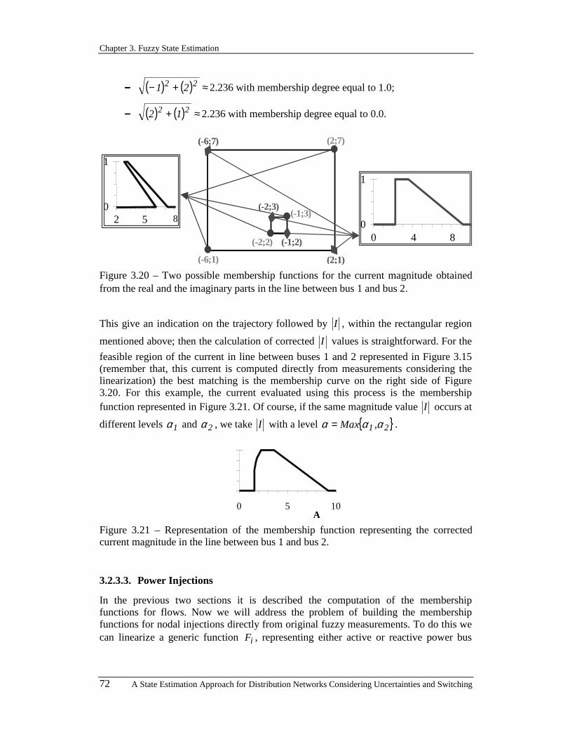
Chapter 3. Fuzzy State Estimation
72 A State Estimation Approach for Distribution Networks Considering Uncertainties and Switching
−−−− ( ) ( ) ≈+− 22 21 2.236 with membership degree equal to 1.0;
−−−− ( ) ( ) ≈+ 22 12 2.236 with membership degree equal to 0.0.
0(-1;3)
(-2;2)
(-6;1)
(-6;7) (2;7)
(2;1)
(-1;2)
(-2;3)
1
2 5 80
1
0 4 8
Figure 3.20 – Two possible membership functions for the current magnitude obtained from the real and the imaginary parts in the line between bus 1 and bus 2.
This give an indication on the trajectory followed by I , within the rectangular region
mentioned above; then the calculation of corrected I values is straightforward. For the
feasible region of the current in line between buses 1 and 2 represented in Figure 3.15 (remember that, this current is computed directly from measurements considering the linearization) the best matching is the membership curve on the right side of Figure 3.20. For this example, the current evaluated using this process is the membership function represented in Figure 3.21. Of course, if the same magnitude value I occurs at
different levels 1α and 2α , we take I with a level { }21 ,Max ααα = .
0 5 10A
Figure 3.21 – Representation of the membership function representing the corrected current magnitude in the line between bus 1 and bus 2.
3.2.3.3. Power Injections
In the previous two sections it is described the computation of the membership functions for flows. Now we will address the problem of building the membership functions for nodal injections directly from original fuzzy measurements. To do this we can linearize a generic function iF , representing either active or reactive power bus
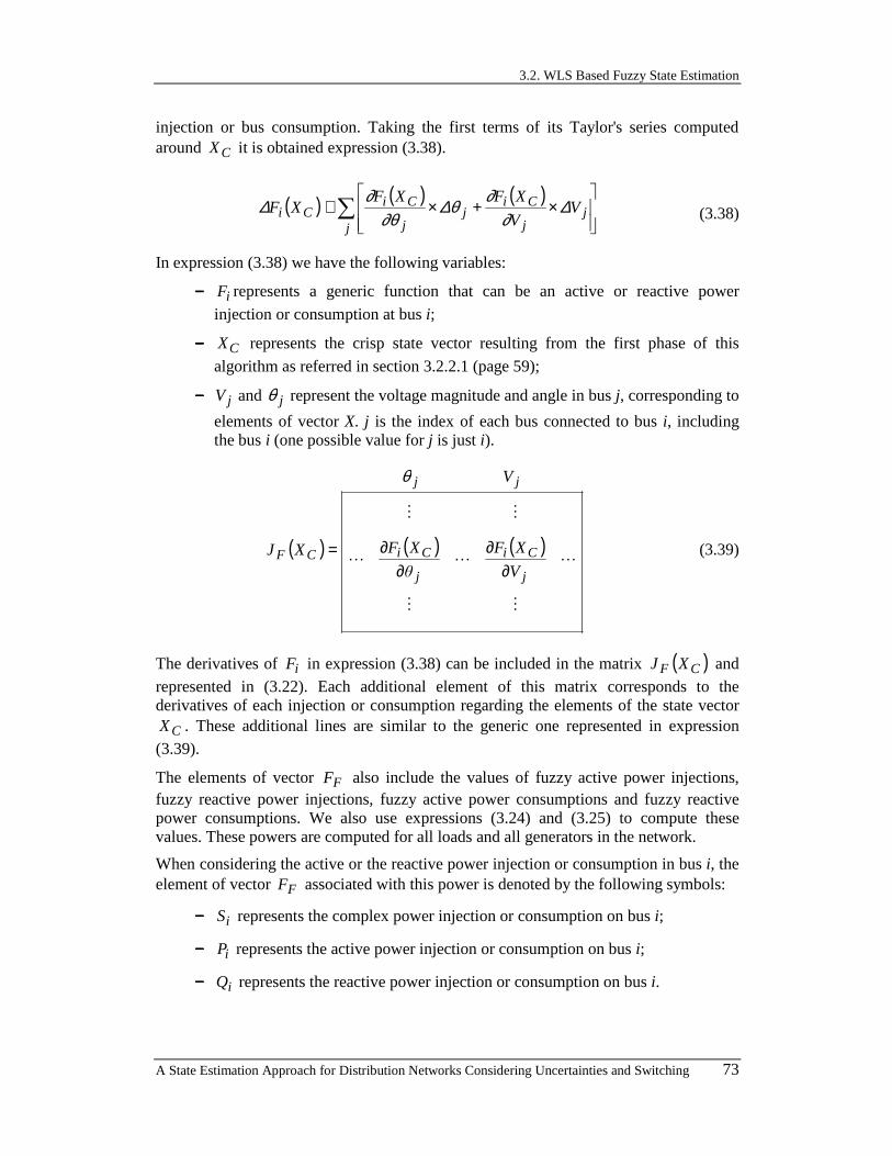
3.2. WLS Based Fuzzy State Estimation
A State Estimation Approach for Distribution Networks Considering Uncertainties and Switching 73
injection or bus consumption. Taking the first terms of its Taylor's series computed around CX it is obtained expression (3.38).
( ) ( ) ( )∑
×+×≅
jj
j
Cij
j
CiCi V
V
XFXFXF ∆
∂∂θ∆
∂θ∂∆ (3.38)
In expression (3.38) we have the following variables:
−−−− iF represents a generic function that can be an active or reactive power
injection or consumption at bus i;
−−−− CX represents the crisp state vector resulting from the first phase of this
algorithm as referred in section 3.2.2.1 (page 59);
−−−− jV and jθ represent the voltage magnitude and angle in bus j, corresponding to
elements of vector X. j is the index of each bus connected to bus i, including the bus i (one possible value for j is just i).
( ) ( ) ( )
MM
LLL
MM
j
Ci
j
Ci
jj
CFV
XF
θXF
V
XJ∂
∂∂
∂=
θ
(3.39)
The derivatives of iF in expression (3.38) can be included in the matrix ( )CF XJ and represented in (3.22). Each additional element of this matrix corresponds to the derivatives of each injection or consumption regarding the elements of the state vector
CX . These additional lines are similar to the generic one represented in expression (3.39).
The elements of vector FF also include the values of fuzzy active power injections, fuzzy reactive power injections, fuzzy active power consumptions and fuzzy reactive power consumptions. We also use expressions (3.24) and (3.25) to compute these values. These powers are computed for all loads and all generators in the network.
When considering the active or the reactive power injection or consumption in bus i, the element of vector FF associated with this power is denoted by the following symbols:
−−−− iS represents the complex power injection or consumption on bus i;
−−−− iP represents the active power injection or consumption on bus i;
−−−− iQ represents the reactive power injection or consumption on bus i.
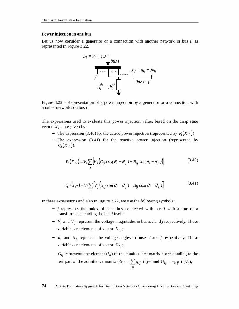
Chapter 3. Fuzzy State Estimation
74 A State Estimation Approach for Distribution Networks Considering Uncertainties and Switching
Power injection in one bus
Let us now consider a generator or a connection with another network in bus i, as represented in Figure 3.22.
bus i
shij
shij jby =
ijijij jbgy +=
iii jQPS +=
… …
line i - j
Figure 3.22 – Representation of a power injection by a generator or a connection with another networks on bus i.
The expressions used to evaluate this power injection value, based on the crisp state vector CX , are given by:
−−−− The expression (3.40) for the active power injection (represented by ( )Ci XP );
−−−− The expression (3.41) for the reactive power injection (represented by ( )Ci XQ ).
( ) ( )[ ]∑ −+−=j
jiijjiijjiCi )sin(B)cos(GVVXP θθθθ (3.40)
( ) ( )[ ]∑ −−−=j
jiijjiijjiCi )cos(B)sin(GVVXQ θθθθ (3.41)
In these expressions and also in Figure 3.22, we use the following symbols:
−−−− j represents the index of each bus connected with bus i with a line or a transformer, including the bus i itself;
−−−− iV and jV represent the voltage magnitudes in buses i and j respectively. These
variables are elements of vector CX ;
−−−− iθ and jθ represent the voltage angles in buses i and j respectively. These
variables are elements of vector CX ;
−−−− ijG represents the element (i,j) of the conductance matrix corresponding to the
real part of the admittance matrix ( ∑≠
=ij
ijii gG if j=i and ijij gG −= if j≠i);
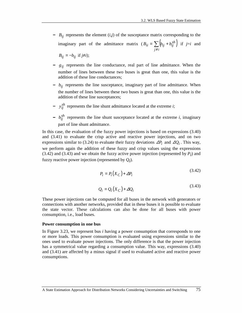
3.2. WLS Based Fuzzy State Estimation
A State Estimation Approach for Distribution Networks Considering Uncertainties and Switching 75
−−−− ijB represents the element (i,j) of the susceptance matrix corresponding to the
imaginary part of the admittance matrix ( ( )∑≠
+=ij
shijijii bbB if j=i and
ijij bB −= if j≠i);
−−−− ijg represents the line conductance, real part of line admittance. When the
number of lines between these two buses is great than one, this value is the addition of these line conductances;
−−−− ijb represents the line susceptance, imaginary part of line admittance. When
the number of lines between these two buses is great than one, this value is the addition of these line susceptances;
−−−− shijy represents the line shunt admittance located at the extreme i;
−−−− shijb represents the line shunt susceptance located at the extreme i, imaginary
part of line shunt admittance.
In this case, the evaluation of the fuzzy power injections is based on expressions (3.40) and (3.41) to evaluate the crisp active and reactive power injections, and on two expressions similar to (3.24) to evaluate their fuzzy deviations iP∆ and iQ∆ . This way, we perform again the addition of these fuzzy and crisp values using the expressions (3.42) and (3.43) and we obtain the fuzzy active power injection (represented by Pi) and fuzzy reactive power injection (represented by Qi).
( ) iCii PXPP ∆+= (3.42)
( ) iCii QXQQ ∆+= (3.43)
These power injections can be computed for all buses in the network with generators or connections with another networks, provided that in these buses it is possible to evaluate the state vector. These calculations can also be done for all buses with power consumption, i.e., load buses.
Power consumption in one bus
In Figure 3.23, we represent bus i having a power consumption that corresponds to one or more loads. This power consumption is evaluated using expressions similar to the ones used to evaluate power injections. The only difference is that the power injection has a symmetrical value regarding a consumption value. This way, expressions (3.40) and (3.41) are affected by a minus signal if used to evaluated active and reactive power consumptions.

Chapter 3. Fuzzy State Estimation
76 A State Estimation Approach for Distribution Networks Considering Uncertainties and Switching
bus i
shij
shij jby =
ijijij jbgy +=iii jQPS += … …
line i - j
Figure 3.23 – Representation of power consumption by one or more loads on bus i.
Power injection and consumption in one bus
In Figure 3.24, it is represented a situation in which, in the same bus, we have power
injection ( inji
inji
inji jQPS += ) and power consumption ( cons
icons
iconsi jQPS += ). In
this case, we must consider the total injected power ( iii jQPS += ) and use the expressions previously presented for a bus power injection. The total injected power is the result of adding all power injections and subtracting all power consumptions, i.e.,
consi
injii SSS −= .
bus i
shij
shij jby =
ijijij jbgy +=
consi
consi
consi jQPS +=
… …
line i - j
inji
inji
inji jQPS +=
Figure 3.24 – Representation of a generic power injection due to generation, connection to another networks or consumptions at bus i.
3.3. RISK INDICES
3.3.1. DEFINITION
The fuzzy state estimation algorithm incorporates fuzzy information in terms of fuzzy numbers. The algorithm described in previous sections translates the uncertainty in input data in the results of the state estimation process. As we have seen these results can correspond to voltage magnitudes, voltage phases, power flows, currents and power injections, all these values being represented by fuzzy numbers.
In particular, this means that the algorithm provides the fuzzy membership function of the current in each branch (that can be or a line or a transformer) represented by a fuzzy number that reflects and is a consequence of admitting uncertainty in measurements. If we want to activate an alarm because the current thermal limit was exceeded we will
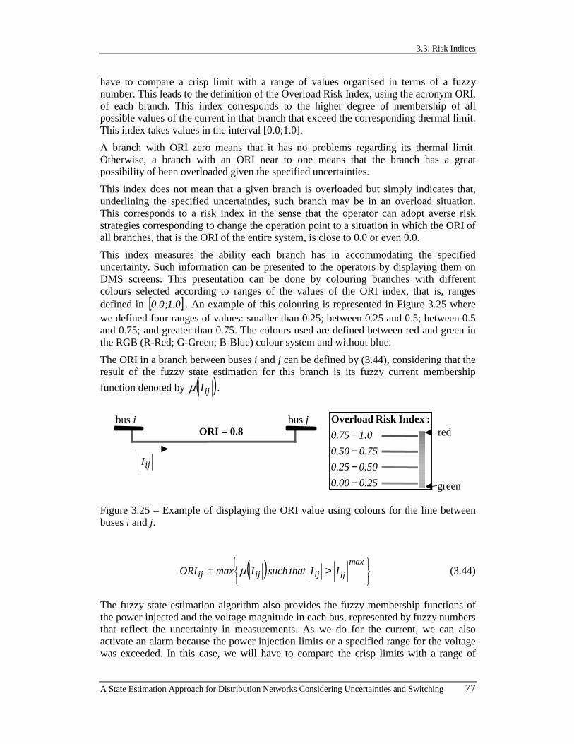
3.3. Risk Indices
A State Estimation Approach for Distribution Networks Considering Uncertainties and Switching 77
have to compare a crisp limit with a range of values organised in terms of a fuzzy number. This leads to the definition of the Overload Risk Index, using the acronym ORI, of each branch. This index corresponds to the higher degree of membership of all possible values of the current in that branch that exceed the corresponding thermal limit. This index takes values in the interval [0.0;1.0].
A branch with ORI zero means that it has no problems regarding its thermal limit. Otherwise, a branch with an ORI near to one means that the branch has a great possibility of been overloaded given the specified uncertainties.
This index does not mean that a given branch is overloaded but simply indicates that, underlining the specified uncertainties, such branch may be in an overload situation. This corresponds to a risk index in the sense that the operator can adopt averse risk strategies corresponding to change the operation point to a situation in which the ORI of all branches, that is the ORI of the entire system, is close to 0.0 or even 0.0.
This index measures the ability each branch has in accommodating the specified uncertainty. Such information can be presented to the operators by displaying them on DMS screens. This presentation can be done by colouring branches with different colours selected according to ranges of the values of the ORI index, that is, ranges defined in [ ]0.1;0.0 . An example of this colouring is represented in Figure 3.25 where we defined four ranges of values: smaller than 0.25; between 0.25 and 0.5; between 0.5 and 0.75; and greater than 0.75. The colours used are defined between red and green in the RGB (R-Red; G-Green; B-Blue) colour system and without blue.
The ORI in a branch between buses i and j can be defined by (3.44), considering that the result of the fuzzy state estimation for this branch is its fuzzy current membership
function denoted by ( )ijIµ .
bus i bus j
ijI
0.8ORI =
25.000.0
50.025.0
75.050.0
0.175.0
−−−−
:Index Risk Overloadred
green
Figure 3.25 – Example of displaying the ORI value using colours for the line between buses i and j.
( )
>=max
ijijijij II that suchImaxORI µ (3.44)
The fuzzy state estimation algorithm also provides the fuzzy membership functions of the power injected and the voltage magnitude in each bus, represented by fuzzy numbers that reflect the uncertainty in measurements. As we do for the current, we can also activate an alarm because the power injection limits or a specified range for the voltage was exceeded. In this case, we will have to compare the crisp limits with a range of
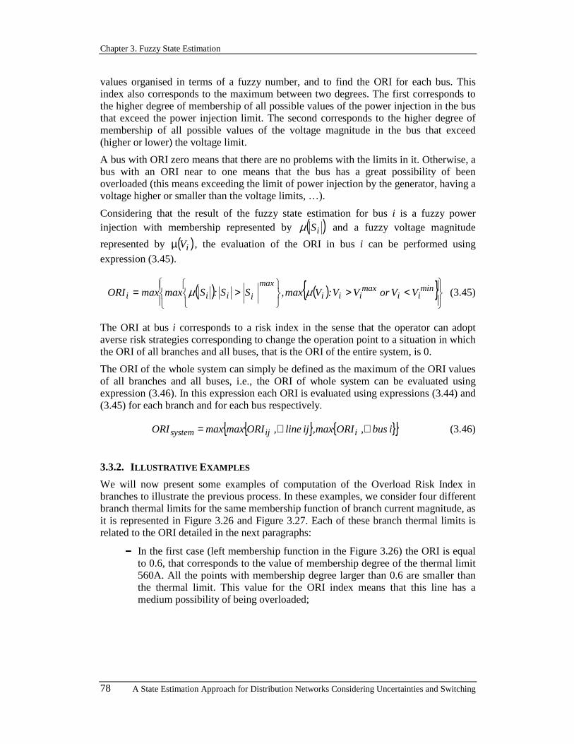
Chapter 3. Fuzzy State Estimation
78 A State Estimation Approach for Distribution Networks Considering Uncertainties and Switching
values organised in terms of a fuzzy number, and to find the ORI for each bus. This index also corresponds to the maximum between two degrees. The first corresponds to the higher degree of membership of all possible values of the power injection in the bus that exceed the power injection limit. The second corresponds to the higher degree of membership of all possible values of the voltage magnitude in the bus that exceed (higher or lower) the voltage limit.
A bus with ORI zero means that there are no problems with the limits in it. Otherwise, a bus with an ORI near to one means that the bus has a great possibility of been overloaded (this means exceeding the limit of power injection by the generator, having a voltage higher or smaller than the voltage limits, …).
Considering that the result of the fuzzy state estimation for bus i is a fuzzy power injection with membership represented by ( )iSµ and a fuzzy voltage magnitude
represented by ( )iVµ , the evaluation of the ORI in bus i can be performed using
expression (3.45).
( ) ( ){ }
<>
>= minii
maxiii
max
iiii VV or VV :Vmax ,SS :SmaxmaxORI µµ (3.45)
The ORI at bus i corresponds to a risk index in the sense that the operator can adopt averse risk strategies corresponding to change the operation point to a situation in which the ORI of all branches and all buses, that is the ORI of the entire system, is 0.
The ORI of the whole system can simply be defined as the maximum of the ORI values of all branches and all buses, i.e., the ORI of whole system can be evaluated using expression (3.46). In this expression each ORI is evaluated using expressions (3.44) and (3.45) for each branch and for each bus respectively.
{ } { }{ }i bus ,ORImax,ij line ,ORImaxmaxORI iijsystem ∀∀= (3.46)
3.3.2. ILLUSTRATIVE EXAMPLES
We will now present some examples of computation of the Overload Risk Index in branches to illustrate the previous process. In these examples, we consider four different branch thermal limits for the same membership function of branch current magnitude, as it is represented in Figure 3.26 and Figure 3.27. Each of these branch thermal limits is related to the ORI detailed in the next paragraphs:
−−−− In the first case (left membership function in the Figure 3.26) the ORI is equal to 0.6, that corresponds to the value of membership degree of the thermal limit 560A. All the points with membership degree larger than 0.6 are smaller than the thermal limit. This value for the ORI index means that this line has a medium possibility of being overloaded;

3.3. Risk Indices
A State Estimation Approach for Distribution Networks Considering Uncertainties and Switching 79
0
1
400 500 600
A
max12I
0.6
560
0
1
400 500 600
A
max34I
0.6
Figure 3.26 – Representation of the membership function for a current magnitude in branches with thermal limits equal to 560A and 500A.
−−−− In the second case (right membership function in the Figure 3.26) the ORI is equal to 1.0, that corresponds to the value of membership degree of points larger than the thermal limit 500A. This means that there is a set of points with great possibility of occurring and therefore a great possibility for the branch to be overloaded. This value for the ORI index means that this line has a very high possibility of being overloaded;
−−−− In the third case (left membership function in the Figure 3.27) the ORI is equal to 1.0, that corresponds to the value of membership degree in points larger than the thermal limit 440A. This means that there is a set of points with great possibility of occurring and therefore a great possibility for the branch to be overloaded. This value for the ORI index means that this branch will be overloaded for every instantiation of the data specified uncertainty;
0
1
400 500 600
A
max23I
4400
1
400 500 600
A
max45I
Figure 3.27 – Representation of the membership function for a current magnitude in branches with thermal limits equal to 440A and 600A.
−−−− In the forth case (right membership function in the Figure 3.27) the ORI is equal to zero, that corresponds to the value of the membership degree related to the thermal limit 600A. All the points with membership degree larger than zero are smaller than the thermal limit. This value for the ORI index means that, despite the specified uncertainty, this line will never be overloaded.
In order to illustrate the computation of the ORI index for buses let us consider the examples in Figure 3.28 and Figure 3.29. In these cases, they are specified ranges for the nodal voltage so that it is possible to measure the risk that voltage has of lying outside this range.
−−−− In the first case (left membership function in the Figure 3.28) the ORI is equal to 0.75, that corresponds to the value of membership degree for the voltage maximum limit 1.1 p.u. All the points with membership degree larger than 0.75 are smaller than the maximum limit and larger than the minimum limit. This
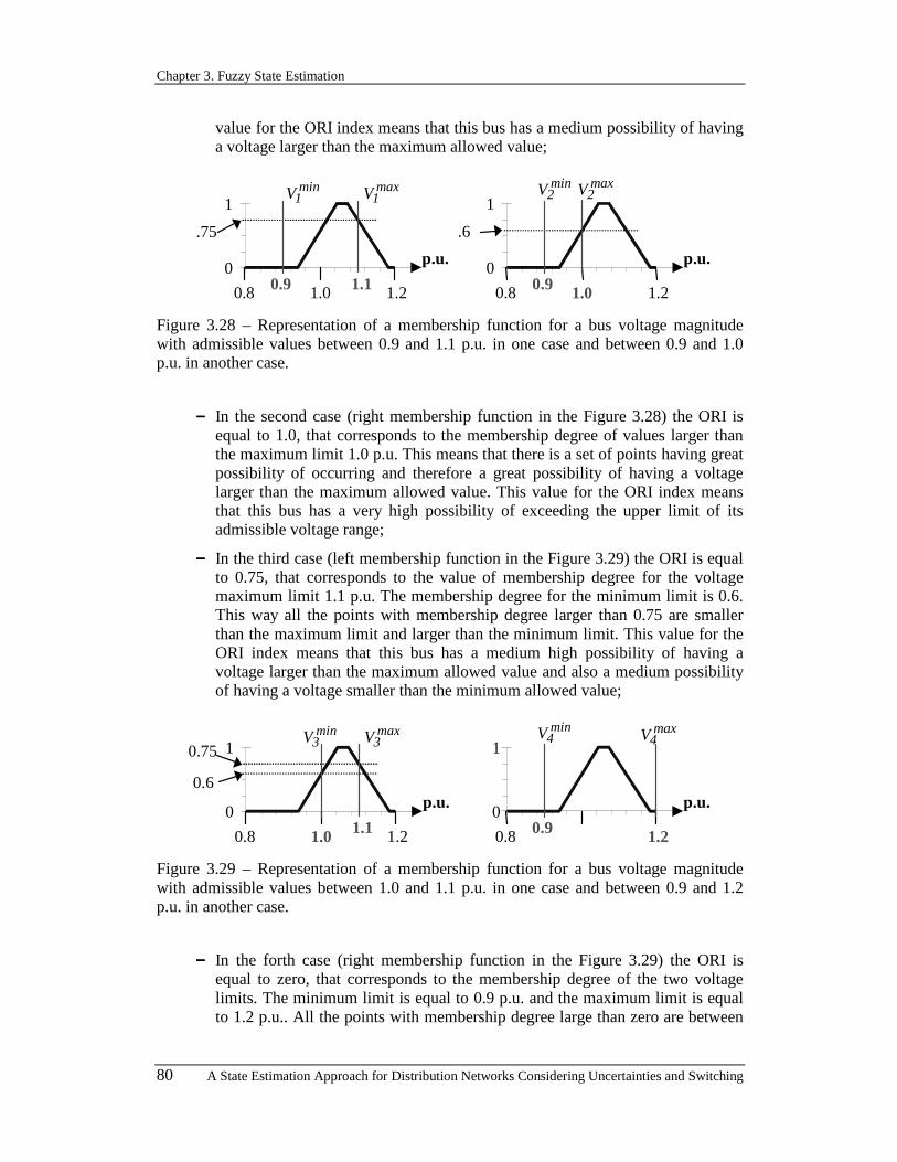
Chapter 3. Fuzzy State Estimation
80 A State Estimation Approach for Distribution Networks Considering Uncertainties and Switching
value for the ORI index means that this bus has a medium possibility of having a voltage larger than the maximum allowed value;
0
1
0.8 1.0 1.2
p.u.
max1V
.75
1.1
min1V
0.90
1
0.8 1.0 1.2
p.u.
max2V
.6
min2V
0.9
Figure 3.28 – Representation of a membership function for a bus voltage magnitude with admissible values between 0.9 and 1.1 p.u. in one case and between 0.9 and 1.0 p.u. in another case.
−−−− In the second case (right membership function in the Figure 3.28) the ORI is equal to 1.0, that corresponds to the membership degree of values larger than the maximum limit 1.0 p.u. This means that there is a set of points having great possibility of occurring and therefore a great possibility of having a voltage larger than the maximum allowed value. This value for the ORI index means that this bus has a very high possibility of exceeding the upper limit of its admissible voltage range;
−−−− In the third case (left membership function in the Figure 3.29) the ORI is equal to 0.75, that corresponds to the value of membership degree for the voltage maximum limit 1.1 p.u. The membership degree for the minimum limit is 0.6. This way all the points with membership degree larger than 0.75 are smaller than the maximum limit and larger than the minimum limit. This value for the ORI index means that this bus has a medium high possibility of having a voltage larger than the maximum allowed value and also a medium possibility of having a voltage smaller than the minimum allowed value;
0
1
0.8 1.0 1.2
p.u.
max3V
0.75
1.1
min3V
0.6
0
1
0.8 1.2
p.u.
max4Vmin
4V
0.9
Figure 3.29 – Representation of a membership function for a bus voltage magnitude with admissible values between 1.0 and 1.1 p.u. in one case and between 0.9 and 1.2 p.u. in another case.
−−−− In the forth case (right membership function in the Figure 3.29) the ORI is equal to zero, that corresponds to the membership degree of the two voltage limits. The minimum limit is equal to 0.9 p.u. and the maximum limit is equal to 1.2 p.u.. All the points with membership degree large than zero are between

3.3. Risk Indices
A State Estimation Approach for Distribution Networks Considering Uncertainties and Switching 81
the two voltage limits. This value for the ORI index means that this bus has null possibility of being in an over or in an under voltage situation.
Finally, we present some examples of the ORI index computation for buses now considering the verification of the power injection limits. To do this they are considered two different limits for the bus power injection for the same membership function of power injection magnitude, as represented in Figure 3.30. Each one of these bus power injection limits has the ORI indicated in the next paragraphs:
−−−− In the first case (left membership function in the Figure 3.30) the ORI in the bus is equal to 0.75, that corresponds to the membership degree of the power injection limit 1100 MVA. All the possible values for the power injection magnitude with membership degree larger than 0.75 are smaller than the power injection limit. This value for the ORI index means that this bus has a medium possibility of its injected power being larger than the maximum allowed value. In other words, it has a medium possibility of being in overload given that the power injection can be related to a generator or a connection with another network;
0
1
800 1000 1200
MVA
max1S
.75
11000
1
800 1000 1200
MVA
max2S
.6
Figure 3.30 – Representation of a membership function example for a bus power injection magnitude with limit of 1100 MVA in one case and 1000 MVA in another case.
−−−− In the second case (right membership function in the Figure 3.30) the ORI in the bus is equal to 1.0, that corresponds to the membership degree of points larger than the power injection limit 1000 MVA. This means that there is a set of points with great possibility of occurring and therefore a great possibility of being overloaded. This value for the ORI index means that this bus has a very high possibility of being overloaded given that it can be a generator or a connection with another network.
Admitting that all the presented examples are included in the same network, the Overload Risk Index for whole system is 1.0, that is the maximum of the 10 indices presented. With this index, the system has lines with a very high possibility of being overloaded, bus voltages with very high possibility of being outside the allowed voltage range and also injection values in some buses that can exceed the maximum limit with very high possibility.
In such situation, the operator would be recommended to change the operation point of the system to a situation in which the ORI index of all branches and all buses, that is the ORI index of the entire system, is closer to 0.0 or even assumes the 0.0 value.

Chapter 3. Fuzzy State Estimation
82 A State Estimation Approach for Distribution Networks Considering Uncertainties and Switching
3.4. CONCLUSIONS In this Chapter we described a State Estimation methodology aiming at identifying the state of distribution networks. The model is highly flexible in terms of the data it can incorporate. This can be traditional real time measurements, fuzzy evaluations and results from load allocation procedures. This means that we enlarged the traditional nature of WLS state estimation algorithms to deal with data having uncertainty.
It should be stressed that in this approach we combine traditional WLS probabilistic algorithms with fuzzy concepts. This reflects our desire to use the most adequate mathematical tools for each particular situation, our purpose to use emergent techniques and our belief that fuzzy concepts, despite very appealing, will not replace probabilistic concepts.
This kind of applications have a large potential of use in the future given that they are more adapted to represent reality in a closer way and that they provide a more complete knowledge about the system in operation. It should be referred that the algorithm is computationally very efficient since, in average, the surplus of execution time when compared with traditional WLS approaches is very low. From several experimental runs, we got an average figure of only more 55% computational time when comparing the developed Fuzzy approach with traditional WLS models. This seems a well reduced price to pay when considering the more complete knowledge about system behaviour that is provided.
3.5. CHAPTER REFERENCES
[1] L. A. Zadeh, “Fuzzy Sets”, Information and Control, Vol. 8, pp. 338-353, August 1965.
[2] E. Comellini, G. Gambelli, U. Magagnoli, M. Silvestri, “Correlations entre puissance et énergie consumée par les charges des réseaux publics de distribution” Proceedings of CIRED 1979.
[3] J. N. Fidalgo, M. Matos, M. T. Ponce de Leão, “Assessing Error Bars in Distribution Load Curve Estimation”, Proceedings of the 7th ICANN, W.Gerstner, A.Germond, M.Hasler, J-D.Nicoud (Eds.), Springer, Lausanne, Switzerland, 1997.
[4] Vladimiro Miranda, Jorge Pereira, J. Tomé Saraiva, “Load Allocation in DMS with a Fuzzy State Estimator”, IEEE Transactions on Power Systems, Vol. 15, No. 2, pp. 529-534, May 2000.
[5] A. Kaufmann, M. M. Gupta, Fuzzy Mathematical Models in Engineering and Management Science, North Holland ed., 1988.
[6] V. Miranda, J. Pereira, J. T. Saraiva, “Experiences in State Estimation Models for Distribution Systems Including Fuzzy Systems”, Proceedings of Stockholm Power Tech, Stockholm, Sweden, June 1995.
[7] V. Miranda, M. Matos, J. T. Saraiva, “Fuzzy Load Flow - New Algorithms Incorporating Uncertain Generation and Load Representation”, 10th PSCC, Graz, August 1990; Proceedings of the 10th PSCC, Butterworths, London, 1990.
A State Estimation Approach for Distribution Networks Considering Uncertainties and Switching 83
4. THE SWITCHING PROBLEM
4.1. DESCRIPTION OF PROBLEM At the beginning of the State Estimation process, it is required to identify the current topology in operation. The identification of the topology in operation means that it could be possible to eliminate all the switching devices and to obtain an equivalent network only including the measurements, buses and branches, and of course, the connections between these elements. In the conventional state estimation algorithms and in other electric network applications, the process that performs this search is named Network Topology Processor.
The main objective of the Network Topology Processor is to find the topology of the network based in the data in the SCADA database that is assumed to contain a complete description of the network model. This description includes the location of metering devices for the bus sections (couplers) and for the switching devices (breakers, switches and sectionalizers). The status of these switching devices can be telemetered or entered manually by system operators.
In conventional state estimation algorithms the topology is processed and fixed before running all the other state estimation functions (observability analysis, main algorithm, bad data analysis, …). This means that network topology is known and the state estimation assumes that the topology is correct. Therefore, the identification of bad data only admits errors in the other measurements and never in the status of switching devices. In this case, the state estimation only uses the network simplified by the topology processor and it is not necessary to know where the switching devices and the measurements devices are located.
There are some power systems, like distribution systems, in which it is not frequently possible to find and to fixe one topology beyond any kind of uncertainty. These difficulties regarding distribution systems are caused by the frequent changes in the topology together with the small number of existing measurement devices. These problems lead to situations in which the topology of the system that is currently in operation is not completely known. In any case, it must be considered one topology to initiate the state estimation process but the formulation should be flexible enough to allow changes in the topology if the initial one will not lead to the best solution. This means that the topology processor must be able to consider that the identification of bad data can find errors in the status of some switching devices.
The bad data analysis applied to the switching device status can be structured in two different classes:
−−−− The first class occurs when one switching device is initiated in the open status and at the end of the process, the best solution includes this switching device in the closed status. Some critical examples of this type of bad data can be: equipment that is considered out of service but is in fact in service, equipment considered operating in different sub-networks but that are in fact in the same sub-network, one part of the network is considered operating under a radial configuration but in fact it has loops, …
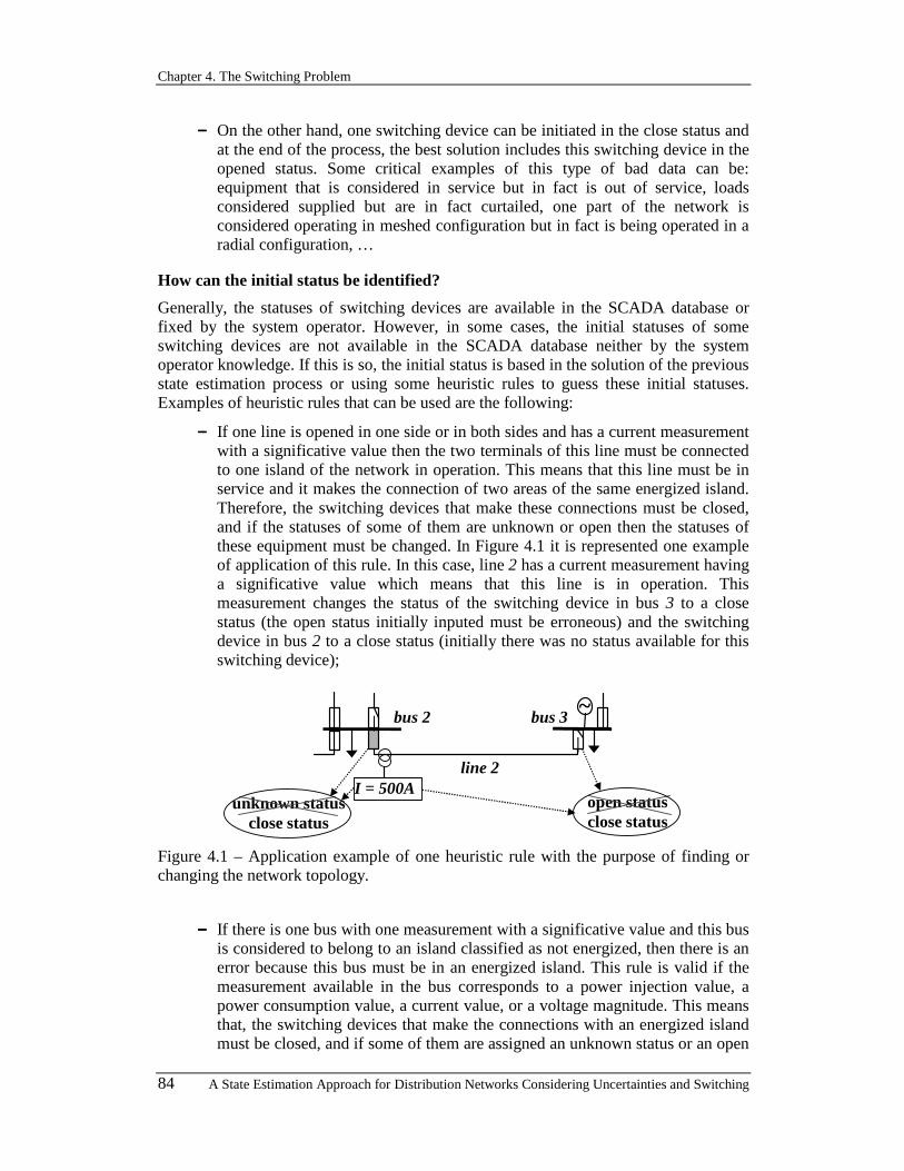
Chapter 4. The Switching Problem
84 A State Estimation Approach for Distribution Networks Considering Uncertainties and Switching
−−−− On the other hand, one switching device can be initiated in the close status and at the end of the process, the best solution includes this switching device in the opened status. Some critical examples of this type of bad data can be: equipment that is considered in service but in fact is out of service, loads considered supplied but are in fact curtailed, one part of the network is considered operating in meshed configuration but in fact is being operated in a radial configuration, …
How can the initial status be identified?
Generally, the statuses of switching devices are available in the SCADA database or fixed by the system operator. However, in some cases, the initial statuses of some switching devices are not available in the SCADA database neither by the system operator knowledge. If this is so, the initial status is based in the solution of the previous state estimation process or using some heuristic rules to guess these initial statuses. Examples of heuristic rules that can be used are the following:
−−−− If one line is opened in one side or in both sides and has a current measurement with a significative value then the two terminals of this line must be connected to one island of the network in operation. This means that this line must be in service and it makes the connection of two areas of the same energized island. Therefore, the switching devices that make these connections must be closed, and if the statuses of some of them are unknown or open then the statuses of these equipment must be changed. In Figure 4.1 it is represented one example of application of this rule. In this case, line 2 has a current measurement having a significative value which means that this line is in operation. This measurement changes the status of the switching device in bus 3 to a close status (the open status initially inputed must be erroneous) and the switching device in bus 2 to a close status (initially there was no status available for this switching device);
|
bus 3 bus 2 ~
line 2
|
I = 500A open status close status
unknown status close status
Figure 4.1 – Application example of one heuristic rule with the purpose of finding or changing the network topology.
−−−− If there is one bus with one measurement with a significative value and this bus is considered to belong to an island classified as not energized, then there is an error because this bus must be in an energized island. This rule is valid if the measurement available in the bus corresponds to a power injection value, a power consumption value, a current value, or a voltage magnitude. This means that, the switching devices that make the connections with an energized island must be closed, and if some of them are assigned an unknown status or an open
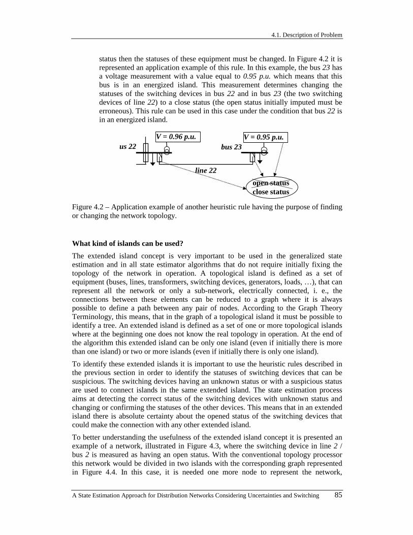
4.1. Description of Problem
A State Estimation Approach for Distribution Networks Considering Uncertainties and Switching 85
status then the statuses of these equipment must be changed. In Figure 4.2 it is represented an application example of this rule. In this example, the bus 23 has a voltage measurement with a value equal to 0.95 p.u. which means that this bus is in an energized island. This measurement determines changing the statuses of the switching devices in bus 22 and in bus 23 (the two switching devices of line 22) to a close status (the open status initially imputed must be erroneous). This rule can be used in this case under the condition that bus 22 is in an energized island.
| |
bus 23 us 22
line 22
V = 0.95 p.u.
open status close status
V = 0.96 p.u.
Figure 4.2 – Application example of another heuristic rule having the purpose of finding or changing the network topology.
What kind of islands can be used?
The extended island concept is very important to be used in the generalized state estimation and in all state estimator algorithms that do not require initially fixing the topology of the network in operation. A topological island is defined as a set of equipment (buses, lines, transformers, switching devices, generators, loads, …), that can represent all the network or only a sub-network, electrically connected, i. e., the connections between these elements can be reduced to a graph where it is always possible to define a path between any pair of nodes. According to the Graph Theory Terminology, this means, that in the graph of a topological island it must be possible to identify a tree. An extended island is defined as a set of one or more topological islands where at the beginning one does not know the real topology in operation. At the end of the algorithm this extended island can be only one island (even if initially there is more than one island) or two or more islands (even if initially there is only one island).
To identify these extended islands it is important to use the heuristic rules described in the previous section in order to identify the statuses of switching devices that can be suspicious. The switching devices having an unknown status or with a suspicious status are used to connect islands in the same extended island. The state estimation process aims at detecting the correct status of the switching devices with unknown status and changing or confirming the statuses of the other devices. This means that in an extended island there is absolute certainty about the opened status of the switching devices that could make the connection with any other extended island.
To better understanding the usefulness of the extended island concept it is presented an example of a network, illustrated in Figure 4.3, where the switching device in line 2 / bus 2 is measured as having an open status. With the conventional topology processor this network would be divided in two islands with the corresponding graph represented in Figure 4.4. In this case, it is needed one more node to represent the network,
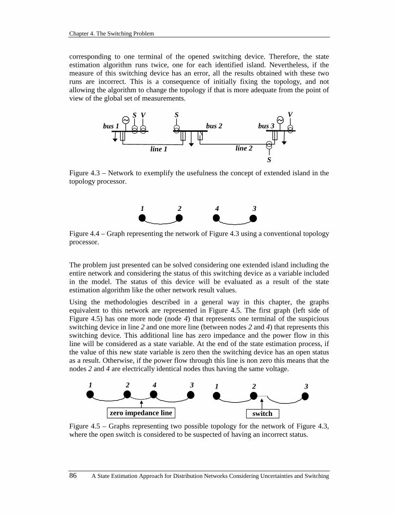
Chapter 4. The Switching Problem
86 A State Estimation Approach for Distribution Networks Considering Uncertainties and Switching
corresponding to one terminal of the opened switching device. Therefore, the state estimation algorithm runs twice, one for each identified island. Nevertheless, if the measure of this switching device has an error, all the results obtained with these two runs are incorrect. This is a consequence of initially fixing the topology, and not allowing the algorithm to change the topology if that is more adequate from the point of view of the global set of measurements.
bus 3bus 2
line 2
S
bus 1
line 1
VS V
S
~~
Figure 4.3 – Network to exemplify the usefulness the concept of extended island in the topology processor.
1 2 4 3
Figure 4.4 – Graph representing the network of Figure 4.3 using a conventional topology processor.
The problem just presented can be solved considering one extended island including the entire network and considering the status of this switching device as a variable included in the model. The status of this device will be evaluated as a result of the state estimation algorithm like the other network result values.
Using the methodologies described in a general way in this chapter, the graphs equivalent to this network are represented in Figure 4.5. The first graph (left side of Figure 4.5) has one more node (node 4) that represents one terminal of the suspicious switching device in line 2 and one more line (between nodes 2 and 4) that represents this switching device. This additional line has zero impedance and the power flow in this line will be considered as a state variable. At the end of the state estimation process, if the value of this new state variable is zero then the switching device has an open status as a result. Otherwise, if the power flow through this line is non zero this means that the nodes 2 and 4 are electrically identical nodes thus having the same voltage.
1 2 4 3
zero impedance line
1 2 3
switch Figure 4.5 – Graphs representing two possible topology for the network of Figure 4.3, where the open switch is considered to be suspected of having an incorrect status.

4.2. Currently Available Solutions for this Problem
A State Estimation Approach for Distribution Networks Considering Uncertainties and Switching 87
The second graph (right side of Figure 4.5) has one more node only if the switch is open. On the other hand, if it is closed, the change is that the state estimation knows that the line 2 has the possibility of being opened in this side. Therefore, one more variable would be added to the vector of state variables. At the end of the state estimation process, the value of this new state variable is zero if the switch has an open status as a result. Otherwise, if the new state variable is one the switch has a close status as a result.
With these examples, it is possible to see that more nodes and more lines will have to be considered in some formulations. Apart from that, it will be necessary to consider more state variables and of different types than the traditional voltages magnitudes and phases. In these cases they will be considered active and reactive power flows as state variables, or switching device variables as state variables, depending on the formulation used. In the next sections, it will describe the changes needed in the state estimation model when the network has a switching device having an unknown status, an open suspicious status or a close suspicious status.
In this type of generalized state estimation the type of state variables is increased and one important rule that should be applied is that the set of state variables should correspond to a minimum set. This means that the number of state variables must be the minimum one while still guaranteeing that all the relevant information about the system can be derived.
In the next sections of this chapter, some available methodologies proposed by some authors to identify the topology throughout the state estimation process are described. In the next section it is described the formulation proposed by Monticelli [1999] on his book [1] that includes ideas already described in references [2], [3] and [4]. In the subsequent section it is described the solution proposed by the author of this Thesis. This approach was described in first place in references [5] and [6] and it was afterwards updated in references [7] and [8].
4.2. CURRENTLY AVAILABLE SOLUTIONS FOR THIS PROBLEM
4.2.1. FORMULATION PROPOSED BY MONTICELLI ET AL
The formulation presented in this section is described in reference [1] and the basic idea of this network topology processor is that a switching device can be modelled as a zero impedance branch. The author names the resulting algorithm to solve the state estimation problem as described in the above-mentioned book, as “Generalized State Estimation”.
4.2.1.1. Modeling switching devices with unknown status
In this section, it is described how one can include in the state estimation algorithm the switching devices with unknown status. To do that, it is considered that in the network where the state estimation is to be run it was identified at least one situation as represented in Figure 4.6. When a switching device with unknown status is present, variables representing the active (denoted by swP ) and the reactive (denoted by swQ ) power flows, through the switching device, are added as state variables. This means that the vector of state variables X has two more elements.

Chapter 4. The Switching Problem
88 A State Estimation Approach for Distribution Networks Considering Uncertainties and Switching
nodew
nodes
MMMM MMMMmeassw
meassw
meassw jQPS +=
nodew
nodes
MMMM MMMMzero impedance line
Figure 4.6 – Generic representation of a switching device with unknown status between node s and w (left figure) and the equivalent graph with a new line (right figure).
In the modelization of one switching device with unknown status there are no constraints related with the voltages in the two terminals, because there is no information about its status. At the end, the status of this switching device is open if the power flows have a zero value as a result. On the other hand, the status is close if the power flows have a non-zero value as a result of the state estimation process.
A consequence of the addition of power flows representing switching devices to the model is related with the measurements available in the neighbourhood of the switching device under analysis.
If it is present in the network a measurement for these new state variables (power flows
denoted by meassw
meassw
meassw jQPS += ) then they must be appropriately included in the
model corresponding to the formulation (3.5) (see expression on page 56). The measurements vector Z has two more elements included on it: one for the active power
measurement through the switching device represented by measswP and another for the
reactive power measurement through the switching device represented by measswQ . In this
case, the expressions used in the referred model and associated to these measurements are (4.1) for the active power flow and (4.2) for the reactive power flow. In these expressions, the variables
swPε and swQε represent the measurement errors, i. e.,
represent the differences between the measured values ( measswP and meas
swQ ) and the true
values of these power flows ( swP and swQ ).
swPswmeassw PP ε+= (4.1)
swQswmeassw QQ ε+= (4.2)
These two new relations are directly expressed in terms of the new state variables swP
and swQ , and not depending on the conventional state variables that are voltage
magnitudes (V) and voltage phases (θ ). Therefore, the zero impedance of the line equivalent to the switching device is never used to evaluate the power flow on it and the numeric problems due to an infinite admittance are circumvented.
Other changes that must be included in the algorithm are related with power injection measurements in the terminal nodes of the switching device, if they exist. The power injections at a node are given by the summation of the power flows in all branches that
4.2. Currently Available Solutions for this Problem
A State Estimation Approach for Distribution Networks Considering Uncertainties and Switching 89
have one terminal in this node. The power flow in the branches that correspond to transmission lines or to transformers is evaluated using the same conventional formulations. These formulations are the expression (3.26) on page 65 for the active power flow and the expression (3.27) on page 65 for the reactive power flow. The power flow in the lines equivalent to switching devices is given directly by the new state variables. Therefore expressions (4.3) and (4.4) are used to relate the active power
injection measurement meassP and the reactive power injection measurement meas
sQ
respectively, in node s with these power injections evaluated using the state variables.
These state variables are now sV , jV , sθ , jθ , swP , swQ and sjP and sjQ only if line
sj is included in the formulation to represent a switching device.
sPswj
sjmeass PPP ε++=∑ (4.3)
sQswj
sjmeass QQQ ε++=∑ (4.4)
On the other hand, expressions (4.5) and (4.6) are used to relate the active power
injection measurement measwP and the reactive power injection measurement meas
wQ
respectively, in node w with these power injections evaluated using the state variables.
In this case, the state variables are wV , jV , wθ , jθ , swP , swQ and wjP and wjQ only
if line wj is included in the formulation to represent a switching device. Notice that the
state variables swP and swQ in these expressions have a minus sign. This is because the
power flow near node w and with the direction from node w to node s (denoted by
wsP and wsQ ) has the symmetrical value of the power flow near node s and with the
direction from node s to node w (denoted by swP and swQ ).
wPswj
wjmeasw PPP ε+−=∑ (4.5)
wQswj
wjmeasw QQQ ε+−=∑ (4.6)
In these expressions the variables sPε ,
sQε , wPε and
wQε represent the errors
affecting the power injection measurements.
4.2.1.2. Modeling opened switching device
Let us now consider that in the network where the state estimation process is running it was identified at least one situation as represented in Figure 4.7 (network on the left side on this figure). This means that in the network there is at least one switching device with
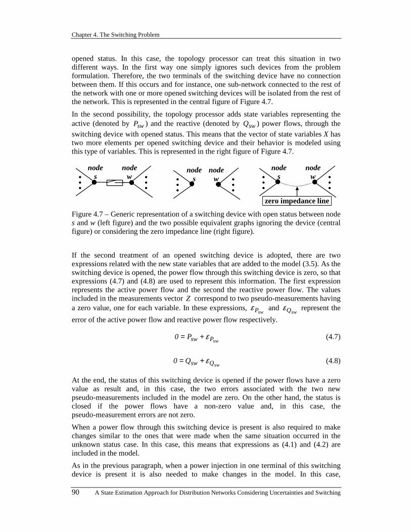
Chapter 4. The Switching Problem
90 A State Estimation Approach for Distribution Networks Considering Uncertainties and Switching
opened status. In this case, the topology processor can treat this situation in two different ways. In the first way one simply ignores such devices from the problem formulation. Therefore, the two terminals of the switching device have no connection between them. If this occurs and for instance, one sub-network connected to the rest of the network with one or more opened switching devices will be isolated from the rest of the network. This is represented in the central figure of Figure 4.7.
In the second possibility, the topology processor adds state variables representing the active (denoted by swP ) and the reactive (denoted by swQ ) power flows, through the
switching device with opened status. This means that the vector of state variables X has two more elements per opened switching device and their behavior is modeled using this type of variables. This is represented in the right figure of Figure 4.7.
node w
node s
MMMM MMMM node
w node
s MMMM MMMM
zero impedance line
node w
node s
MMMM MMMM
Figure 4.7 – Generic representation of a switching device with open status between node s and w (left figure) and the two possible equivalent graphs ignoring the device (central figure) or considering the zero impedance line (right figure).
If the second treatment of an opened switching device is adopted, there are two expressions related with the new state variables that are added to the model (3.5). As the switching device is opened, the power flow through this switching device is zero, so that expressions (4.7) and (4.8) are used to represent this information. The first expression represents the active power flow and the second the reactive power flow. The values included in the measurements vector Z correspond to two pseudo-measurements having a zero value, one for each variable. In these expressions,
swPε and swQε represent the
error of the active power flow and reactive power flow respectively.
swPswP0 ε+= (4.7)
swQswQ0 ε+= (4.8)
At the end, the status of this switching device is opened if the power flows have a zero value as result and, in this case, the two errors associated with the two new pseudo-measurements included in the model are zero. On the other hand, the status is closed if the power flows have a non-zero value and, in this case, the pseudo-measurement errors are not zero.
When a power flow through this switching device is present is also required to make changes similar to the ones that were made when the same situation occurred in the unknown status case. In this case, this means that expressions as (4.1) and (4.2) are included in the model.
As in the previous paragraph, when a power injection in one terminal of this switching device is present it is also needed to make changes in the model. In this case,
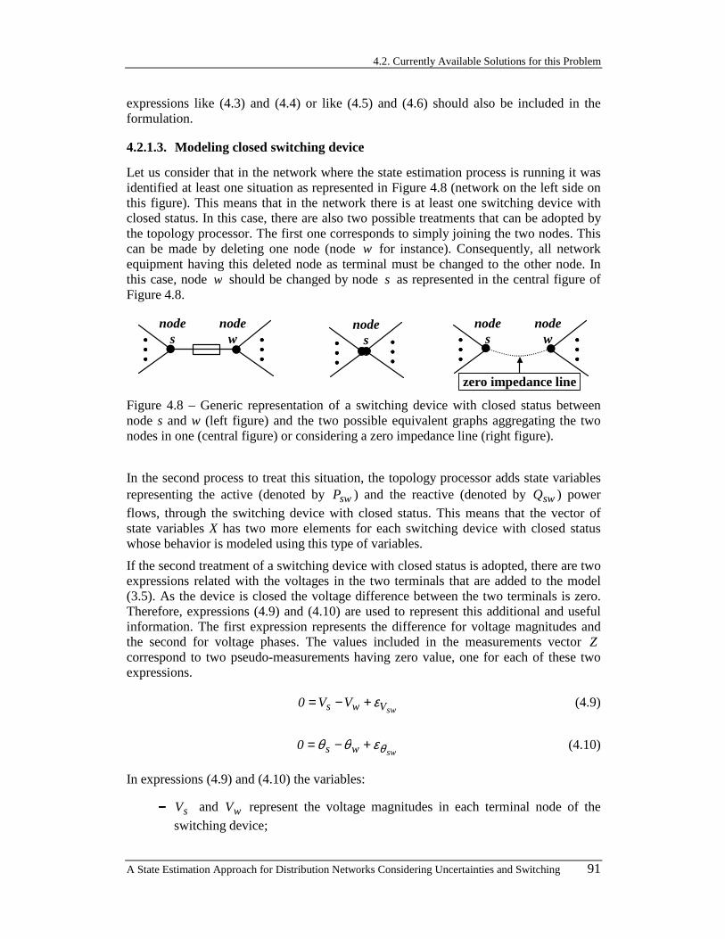
4.2. Currently Available Solutions for this Problem
A State Estimation Approach for Distribution Networks Considering Uncertainties and Switching 91
expressions like (4.3) and (4.4) or like (4.5) and (4.6) should also be included in the formulation.
4.2.1.3. Modeling closed switching device
Let us consider that in the network where the state estimation process is running it was identified at least one situation as represented in Figure 4.8 (network on the left side on this figure). This means that in the network there is at least one switching device with closed status. In this case, there are also two possible treatments that can be adopted by the topology processor. The first one corresponds to simply joining the two nodes. This can be made by deleting one node (node w for instance). Consequently, all network equipment having this deleted node as terminal must be changed to the other node. In this case, node w should be changed by node s as represented in the central figure of Figure 4.8.
node w
node s
MMMM MMMM node
w node
s MMMM MMMM
zero impedance line
node s
MMMM MMMM
Figure 4.8 – Generic representation of a switching device with closed status between node s and w (left figure) and the two possible equivalent graphs aggregating the two nodes in one (central figure) or considering a zero impedance line (right figure).
In the second process to treat this situation, the topology processor adds state variables representing the active (denoted by swP ) and the reactive (denoted by swQ ) power flows, through the switching device with closed status. This means that the vector of state variables X has two more elements for each switching device with closed status whose behavior is modeled using this type of variables.
If the second treatment of a switching device with closed status is adopted, there are two expressions related with the voltages in the two terminals that are added to the model (3.5). As the device is closed the voltage difference between the two terminals is zero. Therefore, expressions (4.9) and (4.10) are used to represent this additional and useful information. The first expression represents the difference for voltage magnitudes and the second for voltage phases. The values included in the measurements vector Z correspond to two pseudo-measurements having zero value, one for each of these two expressions.
swVws VV0 ε+−= (4.9)
swws0 θεθθ +−= (4.10)
In expressions (4.9) and (4.10) the variables:
−−−− sV and wV represent the voltage magnitudes in each terminal node of the
switching device;

Chapter 4. The Switching Problem
92 A State Estimation Approach for Distribution Networks Considering Uncertainties and Switching
−−−− sθ and wθ represent the voltage phases in each terminal node of the switching
device;
−−−− swVε and
swθε represent the error of the voltage magnitude and voltage phase
differences, respectively.
At the end of the state estimation process, the status of this switching device is opened if the power flows through it have a zero value as a result. In this case, the two errors associated with the two new pseudo-measurement included are not zero. On the other hand, the status is closed if the power flows have a non-zero value. In this case, the pseudo-measurement errors are zero.
When a power injection in one terminal of this switching device is present it is also required to make the same changes as the ones considered when the same situation occurred for the unknown status case. In this case, expressions like (4.3) and (4.4) or like (4.5) and (4.6) should also be included in the formulation.
4.3. NEW APPROACH TO ADDRESS THIS PROBLEM In this section, it is presented a methodology to solve the topology identification problem during the state estimation process. This novel approach was described in the first place in reference [5]. Now this approach will be presented, described and justified in a detailed way in the next paragraphs.
In this methodology, the topology unknown problem is addressed by incorporating in the state vector additional variables related with the topology that are called by Topological Variables. This additional type of variables can be used to represent the switching devices where it is not possible to know the current operational status. They can also be used to represent the switching devices for which the current value in the SCADA database is suspicious.
It is important to notice that the time required by the state estimation process to get the solution depends directly on the number of state variables. On the other hand, the number of equations in the problem to solve does not affect in a significative way the computational time. This is because the time spent by the process is very dependent on the time required to invert the gain matrix, and the dimension of this matrix is equal to the number of state variables. The number of equations in the model affects the time required to build this matrix. However, this time is negligible when compared with the time spent to perform the gain matrix inversion.
4.3.1. INCLUSION OF TOPOLOGICAL VARIABLES
The topological variables will be represented by ijD and they can be used to
characterize the knowledge about the branch between bus i and bus j being or not in operation. These variables can also be used to characterize the status of a switching device between bus i and bus j , either in the closed or opened statuses.
These topological variables have an integer and binary nature in the sense that they can only take two values. One possible value for these variables is 1.0 meaning that the branch between bus i and bus j is in operation or the switching device between bus i

4.3. New Approach to Address this Problem
A State Estimation Approach for Distribution Networks Considering Uncertainties and Switching 93
and bus j is closed. Otherwise, these variables take the value 0.0 meaning that the branch is disconnected or the switching device is opened. The incorporation of binary variables in optimization problems increases their complexity leading to non-convex and non-continuous solution sets.
Several formulations treat binary variables by admitting for them a continuous behavior in the interval [ ]0.1;0.0 and rounding them, at the end of the process, to the closer extreme value. This means that the variable during the process can take any value between 0.0 and 0.1 and the result of opened (out of service) or closed (in operation) is dependent on the final rounding. This rounding is done by considering that in the result a value between 0.0 and 5.0 leads to the integer value 0 (opened or out of service). On the other hand, the values between 5.0 and 0.1 lead to the integer value 1 (closed or in operation). This way of treating the binary variables generally has the crucial problem that the optimal solution obtained with continuous variables may not correspond to the optimal solution that would be obtained if the binary nature of these variables was preserved.
Other formulations adopt Branch and Bound type methodologies to treat the binary variables. With these formulations, the optimal solution will be found but they typically require a large number of iterations to do that. For that reason, the time required to obtain the solution is very huge for networks with the dimension of distribution systems. Therefore, these formulations can not be practically used in the determination of the solution for the state estimation problem, because this solution must be founded in real time.
A novel way of addressing this problem corresponds to admit that these variables have a continuous nature imposing, for each of them, a constraint having 0.0 and 0.1 as its solutions. The equation (4.11) can be used for this purpose, in such a way that it is a continuous function and has the possible and desirable solutions. An alternative for this expression is the equation (4.12) that is also a valid function or, in a more general way, one can use equation (4.13). In this case, it must be imposed some constraints to the exponents n and m .
( ) 0xx1 =− (4.11)
( ) 01xx =− (4.12)
0xx mn =− (4.13)
To be used for this purpose equation (4.13) must satisfy one simple criteria related with its exponents. The two exponents of x must be different, the greater exponent must be always an even integer and the smaller index must be always an odd integer. This means that, if n is greater than m then the n must be an even integer and the m must be an odd integer. On the other hand, if m is greater than n then the m must be an even integer and the n must be an odd integer.
The equation (4.11) is a particular case of the equation (4.13) with 1n = and 2m = , and the function associated to this equation is represented in Figure 4.9. This function is a convex one, which is an important property in the sense that the problem to be solved

Chapter 4. The Switching Problem
94 A State Estimation Approach for Distribution Networks Considering Uncertainties and Switching
is an optimization problem. In this way, it is preserved the convex and continuous nature of the problem while imposing that the only feasible solutions are 0.0 and 0.1 .
00 0.5 1 x
( )xx1 −y
zeros
Figure 4.9 – Graphical representation of the function ( )xx1y −= including the zeros of this function.
Additionally, equation (4.12) corresponds to another particular case of equation (4.13) now having 2n = and 1m = . The function associated to this equation is represented in Figure 4.10. This function is also convex and, as well as the previous one, it has only two zeros ( 0.0 and 0.1 ).
00
0.51 x
( )1xx −y zeros
Figure 4.10 – Graphical representation of the function ( )1xxy −= including the zeros of this function.
Furthermore, from our experience the integration of equation (4.11) is more advantageous than equation (4.12) to enforce the values 0.0 or 0.1 for the topological variables. Therefore, this equation will be used in the modelization described in the next paragraphs. Nevertheless, if another equation is used to enforce the binary nature of the continuous variables it is very easy to include it in the model by simply making an analogy with the procedure described in the next paragraphs. It is also presented a parallel modelization to demonstrate how easy this is. This parallel modelization is obtained adopting the equation (4.13) with 8n = and 1m = . This also gives very good results as indicates our experience. The function associated with this new equation is represented in Figure 4.11. This function is also a convex one and, as well as the previous ones, it has only two real zeros ( 0.0 and 0.1 ).
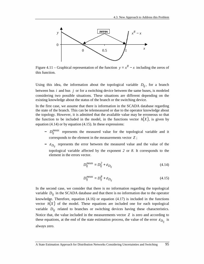
4.3. New Approach to Address this Problem
A State Estimation Approach for Distribution Networks Considering Uncertainties and Switching 95
0
0 0.5 1 x
xx8 −y zeros
Figure 4.11 – Graphical representation of the function xxy 8 −= including the zeros of this function.
Using this idea, the information about the topological variable ijD , for a branch
between bus i and bus j or for a switching device between the same buses, is modeled considering two possible situations. These situations are different depending on the existing knowledge about the status of the branch or the switching device.
In the first case, we assume that there is information in the SCADA database regarding the state of the branch. This can be telemeasured or due to the operator knowledge about the topology. However, it is admitted that the available value may be erroneous so that the function to be included in the model, in the functions vector ( )Xh , is given by equation (4.14) or by equation (4.15). In these expressions:
−−−− measijD represents the measured value for the topological variable and it
corresponds to the element in the measurements vector Z ;
−−−− ijDε represents the error between the measured value and the value of the
topological variable affected by the exponent 2 or 8. It corresponds to the element in the errors vector.
ijD2ij
measij DD ε+= (4.14)
ijD8ij
measij DD ε+= (4.15)
In the second case, we consider that there is no information regarding the topological variable ijD in the SCADA database and that there is no information due to the operator
knowledge. Therefore, equation (4.16) or equation (4.17) is included in the functions vector ( )Xh of the model. These equations are included one for each topological
variable ijD related to branches or switching devices having these characteristics.
Notice that, the value included in the measurements vector Z is zero and according to these equations, at the end of the state estimation process, the value of the error
ijDε is
always zero.

Chapter 4. The Switching Problem
96 A State Estimation Approach for Distribution Networks Considering Uncertainties and Switching
ijD2ijij DD0 ε+−= (4.16)
ijDij8ij DD0 ε+−= (4.17)
Regarding the equations (4.14) and (4.16), or the equations (4.15) and (4.17), one should notice that when the error tends to zero the only feasible solutions are 0.0 or
0.1 . Therefore, we are able to enforce the binary behavior of the topology variables while not compromising the continuous nature of the state estimation problem.
4.3.2. OTHER CHANGES REQUIRED IN THE BASIC MODEL
Apart from the methodology detailed in the previous section, the introduction of topological variables also originates modifications in the existing ( )Xh functions that are already included in the model corresponding to the formulation (3.5) (see expression on page 56). These changes are related with functions regarding branch active and reactive power flows, injected active and reactive powers and currents. These modifications must be done if there is at least a topological variable to represent the operational status of a branch, or at least a topological variable to represent the status of a switching device, or both.
4.3.2.1. Topological variable modeling a branch
In the next paragraphs, we will discuss the inclusion in the model of the topological variable ijD that, in this case, represents the status of the branch between bus i and bus
j . This means that by some reason the operational status of this branch is considered suspicious in terms of being in operation or out of service.
bus jbus i
line i-jmeasij
measij
measij jQPS += meas
jimeasji
measji jQPS +=
measi
measi
measi jQPS += meas
jmeasj
measj jQPS +=
Figure 4.12 – Line represented with unknown status and the inclusion of power measures in the both ends of the line and in the buses.
In Figure 4.12 it is represented an example of one line whose the operational status is unknown, because the two switching devices are assigned an unknown status. According to this figure, there are active and reactive power measurements for both extremes of this line and, in this section, it is discussed the inclusion of each one of this measurements in the model. Therefore, in the next paragraphs will discuss the changes to be implemented when they are available active and reactive power flow measurements in each extremity of a suspicious branch. They are also analyzed the
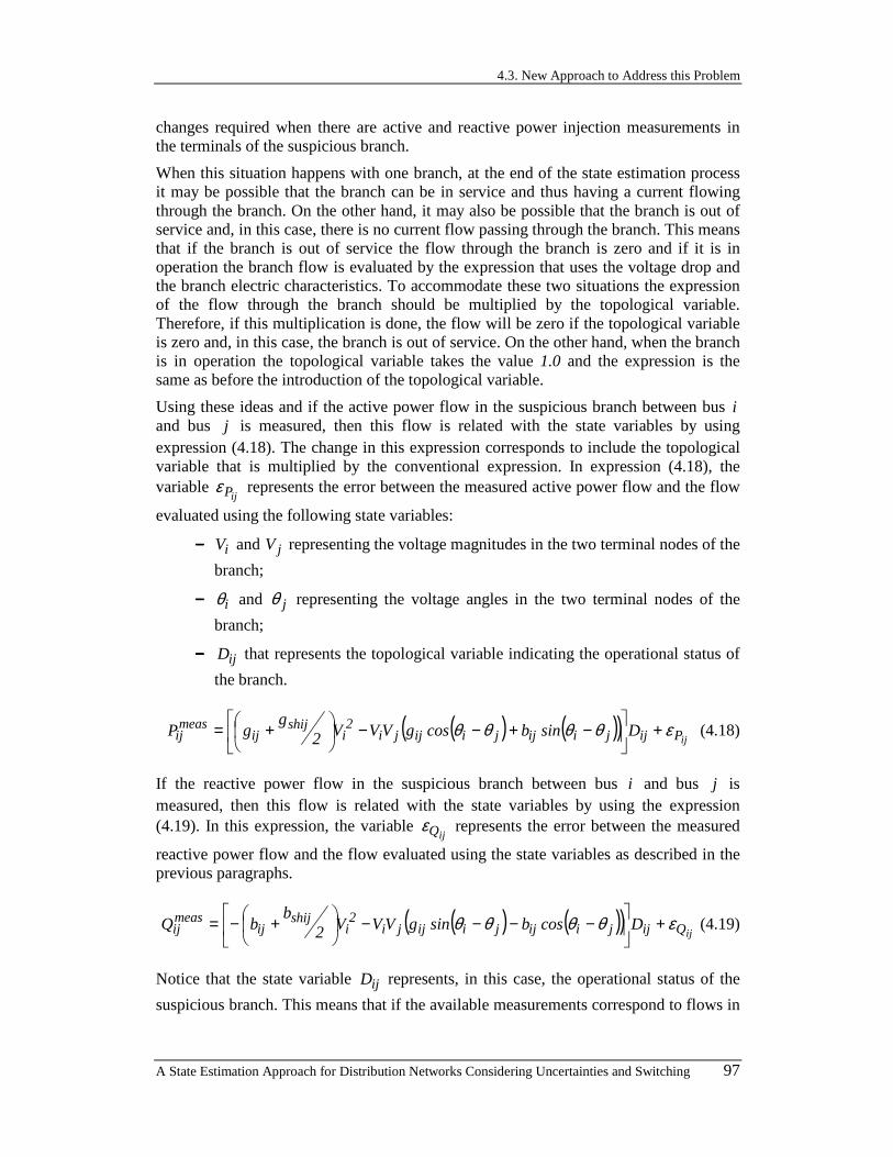
4.3. New Approach to Address this Problem
A State Estimation Approach for Distribution Networks Considering Uncertainties and Switching 97
changes required when there are active and reactive power injection measurements in the terminals of the suspicious branch.
When this situation happens with one branch, at the end of the state estimation process it may be possible that the branch can be in service and thus having a current flowing through the branch. On the other hand, it may also be possible that the branch is out of service and, in this case, there is no current flow passing through the branch. This means that if the branch is out of service the flow through the branch is zero and if it is in operation the branch flow is evaluated by the expression that uses the voltage drop and the branch electric characteristics. To accommodate these two situations the expression of the flow through the branch should be multiplied by the topological variable. Therefore, if this multiplication is done, the flow will be zero if the topological variable is zero and, in this case, the branch is out of service. On the other hand, when the branch is in operation the topological variable takes the value 1.0 and the expression is the same as before the introduction of the topological variable.
Using these ideas and if the active power flow in the suspicious branch between bus i and bus j is measured, then this flow is related with the state variables by using expression (4.18). The change in this expression corresponds to include the topological variable that is multiplied by the conventional expression. In expression (4.18), the variable
ijPε represents the error between the measured active power flow and the flow
evaluated using the following state variables:
−−−− iV and jV representing the voltage magnitudes in the two terminal nodes of the
branch;
−−−− iθ and jθ representing the voltage angles in the two terminal nodes of the
branch;
−−−− ijD that represents the topological variable indicating the operational status of
the branch.
( ) ( )( )ijPijjiijjiijji
2i
shijij
measij DsinbcosgVVV2
ggP εθθθθ +
−+−−
+= (4.18)
If the reactive power flow in the suspicious branch between bus i and bus j is measured, then this flow is related with the state variables by using the expression (4.19). In this expression, the variable
ijQε represents the error between the measured
reactive power flow and the flow evaluated using the state variables as described in the previous paragraphs.
( ) ( )( )ijQijjiijjiijji
2i
shijij
measij DcosbsingVVV2
bbQ εθθθθ +
−−−−
+−= (4.19)
Notice that the state variable ijD represents, in this case, the operational status of the
suspicious branch. This means that if the available measurements correspond to flows in

Chapter 4. The Switching Problem
98 A State Estimation Approach for Distribution Networks Considering Uncertainties and Switching
the opposite direction it can be used the same state variable ijD , because the values of
the variable jiD and of the variable ijD are the same. Therefore, the model only uses
one of them, in this case the topological variable ijD . The expressions (4.20) and (4.21)
represent the modifications that must be done in the relations between the power flow measurements in a branch and the state variables for ji flow measurements. Of course these expressions are only used when the active or the reactive flows are measured in the direction from node j to node i .
( ) ( )( )jiPijijjiijjiji
2j
shjiji
measji DsinbcosgVVV2
ggP εθθθθ +
−+−−
+= (4.20)
( ) ( )( )jiQijijjiijjiji
2j
shjiji
measji DcosbsingVVV2
bbQ εθθθθ +
−−−−
+−= (4.21)
If measurements of active or reactive power injections are available in the bus i , then the modifications due to the introduction of the new topological variables are the represented in the expressions (4.22) and (4.23). These expressions are used to express
the active power injected measurement (represented by measiP ) and the reactive power
injected measurement (represented by measiQ ) in the bus i with the corresponding state
variables. In these expressions, the variables iPε and
iQε represent the errors between
the measured power injection and the injection evaluated using the state variables.
( ) ( )( )iP
sissiissiissi
2i
shisis
measi DsinbcosgVVV2
ggP εθθθθ +
−+−−
+=∑
isP
(4.22)
( ) ( )( )iQ
sissiissiissi
2i
shisis
measi DcosbsingVVV2
bbQ εθθθθ +
−−−−
+−=∑
isQ
(4.23)
It should be referred that the index s in these expressions always corresponds to a terminal bus of one branch that leaves bus i . Since it is not known a priori what branches are in operation, that is, which ones are effectively connected to bus i , it is not possible to evaluate the ( )i,i diagonal element of the admittance matrix. To overcome this problem, the index s in the summations in expressions (4.22) and (4.23) will never take value i . The terms that would determine the referred ( )i,i diagonal element are
multiplied by the topological variable isD . This means that, given the lack of

4.3. New Approach to Address this Problem
A State Estimation Approach for Distribution Networks Considering Uncertainties and Switching 99
knowledge regarding the status of the branches, the iig element is given by expression
(4.24) and the iib element is given by expression (4.25).
∑
+−=
sis
shisisii D2
ggg (4.24)
∑
+=
sis
shisisii D2
bbb (4.25)
From this moment onwards, it will be used a compacted notation to represent the expressions to evaluate the power flows in one branch based in the branch characteristics and in the voltages and phases in the two terminal buses. The first compaction corresponds to use isP to represent the expression to evaluate the active
power flow in the branch between bus i and bus s . In a similar way isQ represents the expression to evaluate the reactive power flow in the same branch.
Until now, for any power injection measurements we assumed that all branches that leave one bus are suspicious. However, some of them can be suspicious while others are not under this situation. Therefore, the expressions to model these measures should be a combination between the traditional expressions and the ones presented in this chapter. Expressions (4.26) and (4.27) represent this combination for the active power injection measurement and for the reactive power injection measurement, respectively. In these expressions, the index s represents the buses in such way that the branches between bus i and bus s are considered suspicious and the index k represents the terminal nodes of all other branches under the condition they are connected to bus i .
[ ] [ ]iP
kik
sisis
measi PDPP ε++= ∑∑ (4.26)
[ ] [ ]iQ
kik
sisis
measi QDQQ ε++= ∑∑ (4.27)
4.3.2.2. Topological variable modeling a switching device
In the next paragraphs it is discussed the inclusion in the model of the topological variable ijD that, in this case, represents the status of the switching device between bus
i and bus j . This means that by some reason the status of this switching device is considered suspicious in terms of being opened or closed or simply the state is considered unknown.
In Figure 4.13 it is represented an example of one switching device whose status is unknown. The possible status for a switching device can be also suspicious with opened status, or suspicious with closed status or not suspicious. The case of not being suspicious is not important to be included in the model for the reason that it is eliminated by the initial network topology processor. In the next paragraphs when the open status is assigned to a switching device we mean that the status of the device is

Chapter 4. The Switching Problem
100 A State Estimation Approach for Distribution Networks Considering Uncertainties and Switching
open but it is suspicious by some reason. The same meaning has the close status. It signifies that the status of the switching device is close but it is also suspicious.
bus jbus i
switching device
measi
measi
measi jQPS += meas
jmeasj
measj jQPS +=
Figure 4.13 – Part of a network with a switching device that has an unknown status and with power measures in the both terminal buses of the switching device.
In Figure 4.13 they are represented measures of power injections in both buses and the inclusion of these measurements in the model is the main topic addressed in this section. Therefore, in the next paragraphs they will be discussed the changes to be implemented when there are active and reactive power injection measurements in the terminals of the switching devices with unknown status, closed status or opened status.
When this happens with one switching device, at the end of the state estimation process it may be possible that the switching device can be opened and therefore the two buses are disconnected. On the other hand, it may also be possible that the switching device can be closed and, in this case, the two buses are connected and are electrically the same bus. This electrical connection or disconnection can be represented in the mathematical formulation by expressions (4.28) and (4.29), one for the voltage magnitude and the other for the voltage angle. These expressions represent the voltage difference between the two switching device terminals, buses i and j , and at the end of the state estimation process, the two expressions are always true. This is because the switching device is closed and the voltage in the two terminals is the same ( 0VV ji =− and 0ji =−θθ ) or
it is opened and the topological variable is zero ( 0Dij = ).
( )ijV0ijji DVV0 ε+−= (4.28)
( )ij0ijji D0 θεθθ +−= (4.29)
Another important characteristic of the status of a switching device is that if the switching device is opened the power injection in each bus only corresponds to the addition of all power flows in all branches leaving that bus. On the other hand, when the switching device is closed the power injection in the connected two buses is the addition of all power flows in all branches leaving the two buses all together. Therefore, the voltage in the two buses has the same value.
In the next paragraphs we will explain the other changes required in the model. We will detail these changes for the active power measurements since the changes for the reactive power measurements are similar.
To describe all the modifications that must be introduced in the model when the network has one switching device on these conditions we will consider the three
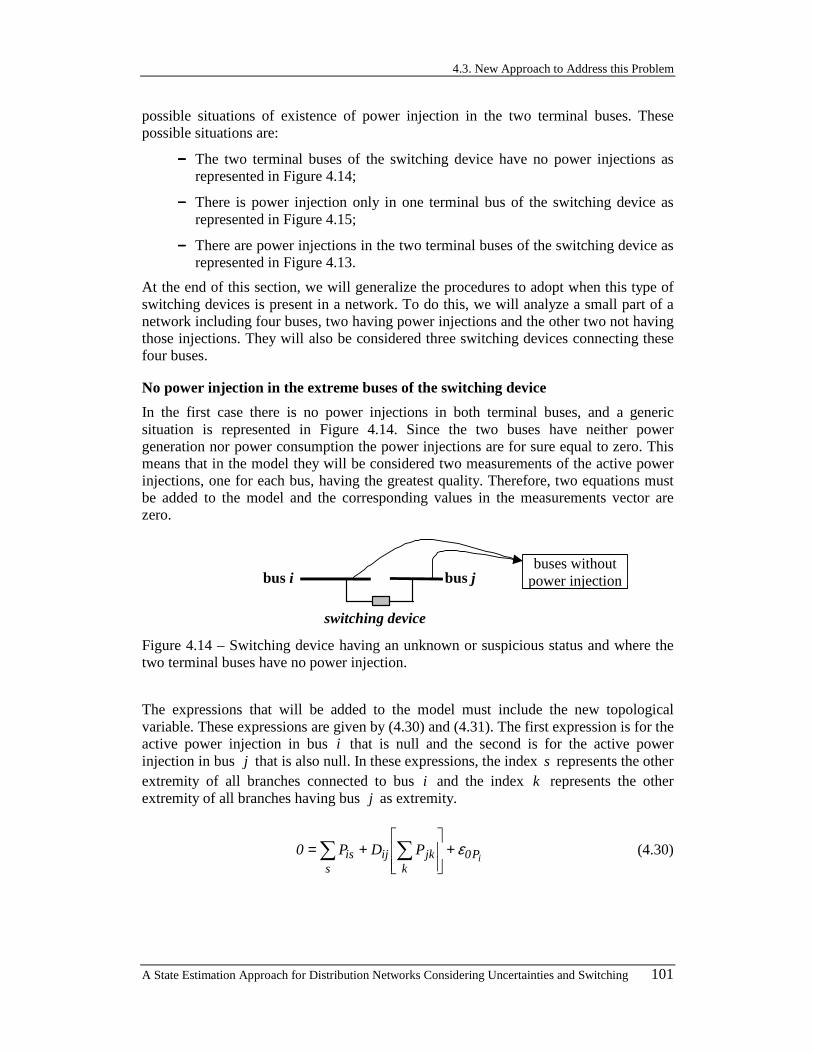
4.3. New Approach to Address this Problem
A State Estimation Approach for Distribution Networks Considering Uncertainties and Switching 101
possible situations of existence of power injection in the two terminal buses. These possible situations are:
−−−− The two terminal buses of the switching device have no power injections as represented in Figure 4.14;
−−−− There is power injection only in one terminal bus of the switching device as represented in Figure 4.15;
−−−− There are power injections in the two terminal buses of the switching device as represented in Figure 4.13.
At the end of this section, we will generalize the procedures to adopt when this type of switching devices is present in a network. To do this, we will analyze a small part of a network including four buses, two having power injections and the other two not having those injections. They will also be considered three switching devices connecting these four buses.
No power injection in the extreme buses of the switching device
In the first case there is no power injections in both terminal buses, and a generic situation is represented in Figure 4.14. Since the two buses have neither power generation nor power consumption the power injections are for sure equal to zero. This means that in the model they will be considered two measurements of the active power injections, one for each bus, having the greatest quality. Therefore, two equations must be added to the model and the corresponding values in the measurements vector are zero.
bus jbus i
switching device
buses withoutpower injection
Figure 4.14 – Switching device having an unknown or suspicious status and where the two terminal buses have no power injection.
The expressions that will be added to the model must include the new topological variable. These expressions are given by (4.30) and (4.31). The first expression is for the active power injection in bus i that is null and the second is for the active power injection in bus j that is also null. In these expressions, the index s represents the other extremity of all branches connected to bus i and the index k represents the other extremity of all branches having bus j as extremity.
iP0k
jkijs
is PDP0 ε+
+= ∑∑ (4.30)
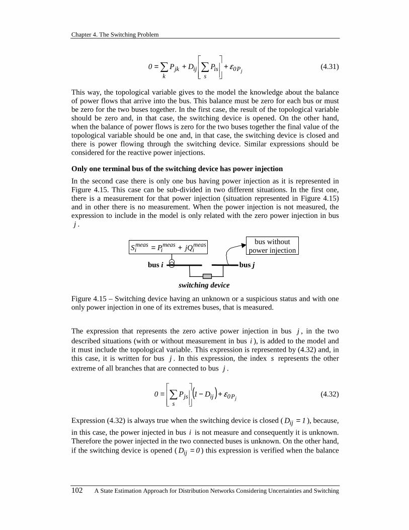
Chapter 4. The Switching Problem
102 A State Estimation Approach for Distribution Networks Considering Uncertainties and Switching
jP0s
isijk
jk PDP0 ε+
+= ∑∑ (4.31)
This way, the topological variable gives to the model the knowledge about the balance of power flows that arrive into the bus. This balance must be zero for each bus or must be zero for the two buses together. In the first case, the result of the topological variable should be zero and, in that case, the switching device is opened. On the other hand, when the balance of power flows is zero for the two buses together the final value of the topological variable should be one and, in that case, the switching device is closed and there is power flowing through the switching device. Similar expressions should be considered for the reactive power injections.
Only one terminal bus of the switching device has power injection
In the second case there is only one bus having power injection as it is represented in Figure 4.15. This case can be sub-divided in two different situations. In the first one, there is a measurement for that power injection (situation represented in Figure 4.15) and in other there is no measurement. When the power injection is not measured, the expression to include in the model is only related with the zero power injection in bus j .
bus jbus i
switching device
measi
measi
measi jQPS +=
bus withoutpower injection
Figure 4.15 – Switching device having an unknown or a suspicious status and with one only power injection in one of its extremes buses, that is measured.
The expression that represents the zero active power injection in bus j , in the two described situations (with or without measurement in bus i ), is added to the model and it must include the topological variable. This expression is represented by (4.32) and, in this case, it is written for bus j . In this expression, the index s represents the other extreme of all branches that are connected to bus j .
( )jP0ij
sjs D1P0 ε+−
= ∑ (4.32)
Expression (4.32) is always true when the switching device is closed ( 1Dij = ), because,
in this case, the power injected in bus i is not measure and consequently it is unknown. Therefore the power injected in the two connected buses is unknown. On the other hand, if the switching device is opened ( 0Dij = ) this expression is verified when the balance
4.3. New Approach to Address this Problem
A State Estimation Approach for Distribution Networks Considering Uncertainties and Switching 103
of all power flows that arrive to bus j is zero. This means that the power injection in this bus is zero, and this is the correct solution because bus i is isolated from bus j .
Finally, regarding the active power injection, its expression must be included in the model provided that injection is measured. The expression for bus i is given by (4.33) and it includes the new topological variable. In this expression, the index s represents the other extreme of all branches connected to bus i and the index k represents the other extreme of all branches connected to bus j .
iPk
jkijs
ismeas
i PDPP ε+
+= ∑∑ (4.33)
Expression (4.33) represents the balance of all power flows that arrive only to bus i when the switching device is opened ( 0Dij = ), apart from the error variable
iPε . On
the other hand, if the switching device is closed ( 1Dij = ) this expression is verified,
apart from the error variable iPε , when the balance of all power flows that arrive to the
bus i and to the bus j is the measured value measiP . This means that the balance of all
power flows in the lines with an extreme equal to the bus j (∑k
jkP ) can be zero or not.
This corresponds to the correct situation that can physically happen in real systems. Similar expressions should be considered for the reactive power injections.
The two terminal buses of the switching device have power injections
In the third case there are power injections in the two buses. This case can be represented by Figure 4.13 and it can also be sub-divided in three different situations:
−−−− None of the two power injections are measured;
−−−− Both power injections are measured in each of the two buses, similar to the situation represented in Figure 4.13;
−−−− Finally, there is only one available power injection measurement (situation represented in Figure 4.16).
When the power injections are not measured, there are no additional expressions to be included in the model regarding the power injections in the buses.
In the second situation, when the two power injections are measured, it is necessary to add to the state vector an extra state variable ijP to represent the power flow through the
switching device. Together with this new state variable it is necessary to include in the model three expressions, one for each power injection measurement (expressions (4.34) and (4.35)) and the other for the relation between the new state variable and the topological variable (expression (4.36)).
iPijs
ismeas
i PPP ε++=∑ (4.34)
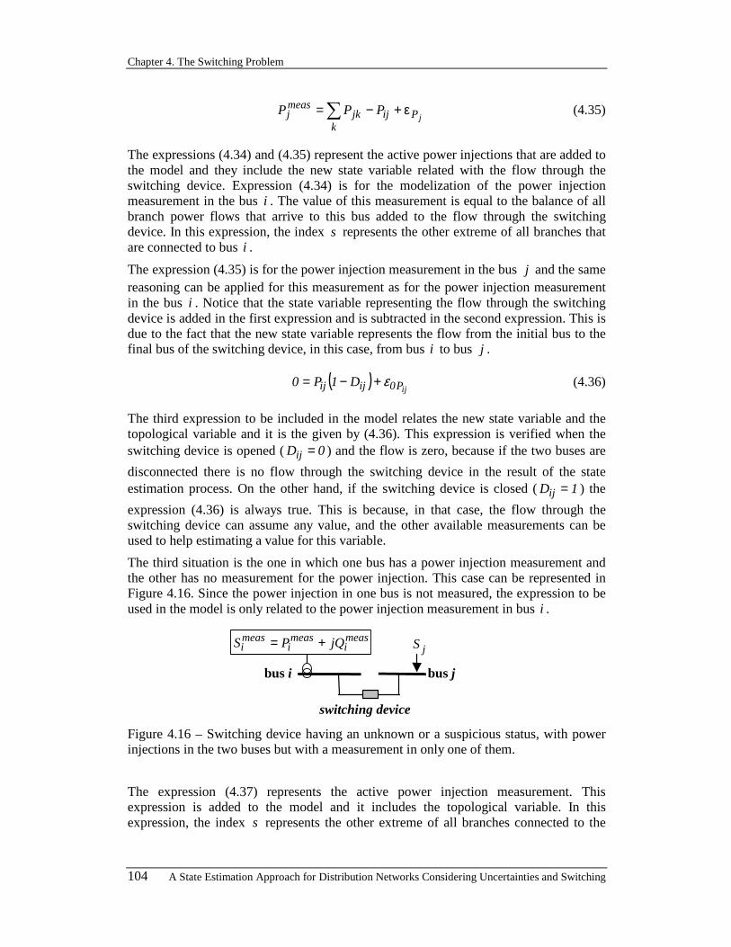
Chapter 4. The Switching Problem
104 A State Estimation Approach for Distribution Networks Considering Uncertainties and Switching
jPijk
jkmeasj PPP ε+−=∑ (4.35)
The expressions (4.34) and (4.35) represent the active power injections that are added to the model and they include the new state variable related with the flow through the switching device. Expression (4.34) is for the modelization of the power injection measurement in the bus i . The value of this measurement is equal to the balance of all branch power flows that arrive to this bus added to the flow through the switching device. In this expression, the index s represents the other extreme of all branches that are connected to bus i .
The expression (4.35) is for the power injection measurement in the bus j and the same reasoning can be applied for this measurement as for the power injection measurement in the bus i . Notice that the state variable representing the flow through the switching device is added in the first expression and is subtracted in the second expression. This is due to the fact that the new state variable represents the flow from the initial bus to the final bus of the switching device, in this case, from bus i to bus j .
( )ijP0ijij D1P0 ε+−= (4.36)
The third expression to be included in the model relates the new state variable and the topological variable and it is the given by (4.36). This expression is verified when the switching device is opened ( 0Dij = ) and the flow is zero, because if the two buses are
disconnected there is no flow through the switching device in the result of the state estimation process. On the other hand, if the switching device is closed ( 1Dij = ) the
expression (4.36) is always true. This is because, in that case, the flow through the switching device can assume any value, and the other available measurements can be used to help estimating a value for this variable.
The third situation is the one in which one bus has a power injection measurement and the other has no measurement for the power injection. This case can be represented in Figure 4.16. Since the power injection in one bus is not measured, the expression to be used in the model is only related to the power injection measurement in bus i .
bus jbus i
switching device
measi
measi
measi jQPS += jS
Figure 4.16 – Switching device having an unknown or a suspicious status, with power injections in the two buses but with a measurement in only one of them.
The expression (4.37) represents the active power injection measurement. This expression is added to the model and it includes the topological variable. In this expression, the index s represents the other extreme of all branches connected to the
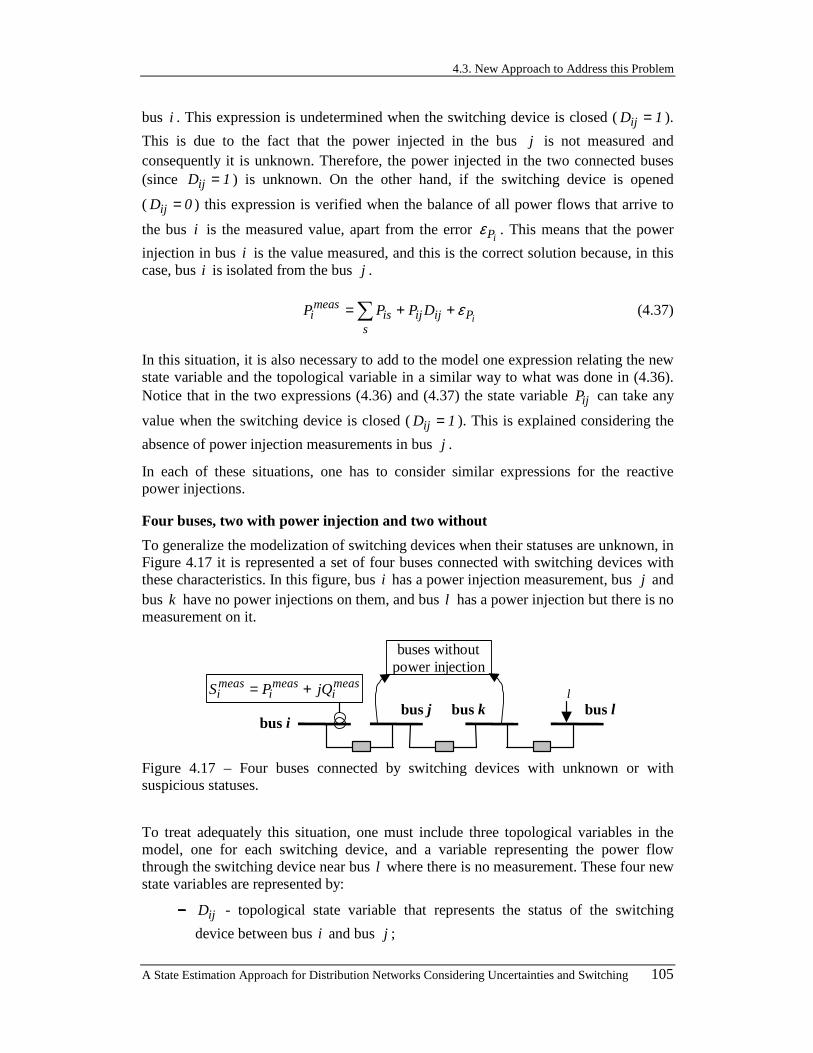
4.3. New Approach to Address this Problem
A State Estimation Approach for Distribution Networks Considering Uncertainties and Switching 105
bus i . This expression is undetermined when the switching device is closed ( 1Dij = ).
This is due to the fact that the power injected in the bus j is not measured and consequently it is unknown. Therefore, the power injected in the two connected buses (since 1Dij = ) is unknown. On the other hand, if the switching device is opened
( 0Dij = ) this expression is verified when the balance of all power flows that arrive to
the bus i is the measured value, apart from the error iPε . This means that the power
injection in bus i is the value measured, and this is the correct solution because, in this case, bus i is isolated from the bus j .
iPijijs
ismeas
i DPPP ε++=∑ (4.37)
In this situation, it is also necessary to add to the model one expression relating the new state variable and the topological variable in a similar way to what was done in (4.36). Notice that in the two expressions (4.36) and (4.37) the state variable ijP can take any
value when the switching device is closed ( 1Dij = ). This is explained considering the
absence of power injection measurements in bus j .
In each of these situations, one has to consider similar expressions for the reactive power injections.
Four buses, two with power injection and two without
To generalize the modelization of switching devices when their statuses are unknown, in Figure 4.17 it is represented a set of four buses connected with switching devices with these characteristics. In this figure, bus i has a power injection measurement, bus j and bus k have no power injections on them, and bus l has a power injection but there is no measurement on it.
bus j bus i
measi
measi
measi jQPS +=
buses without power injection
bus l bus k l
Figure 4.17 – Four buses connected by switching devices with unknown or with suspicious statuses.
To treat adequately this situation, one must include three topological variables in the model, one for each switching device, and a variable representing the power flow through the switching device near bus l where there is no measurement. These four new state variables are represented by:
−−−− ijD - topological state variable that represents the status of the switching
device between bus i and bus j ;
Chapter 4. The Switching Problem
106 A State Estimation Approach for Distribution Networks Considering Uncertainties and Switching
−−−− jkD - topological state variable that represents the status of the switching
device between bus j and bus k ;
−−−− klD - topological state variable that represents the status of the switching
device between bus k and bus l ;
−−−− klP - new state variable that represents the active power flow through the
switching device between bus k and bus l , and with this conventional direction. In this case, there is one only constraint on the value that this variable can take because, although there is a power injection on bus l , lS is not
measured. This constraint imposes that the value of klP is zero if the switching
device between bus k and bus l is opened, in the final result of the state estimation algorithm.
Several equations must be added to the model to represent the information available about the measurements and the zero injections in buses j and k . The first type of equations to be added to the formulation aim at representing the electrical connection or disconnection of each pair of buses as a result of final status of the intermediate switching device. These equations are similar to (4.28) and (4.29) but for clarity purposes we will now detail them:
−−−− equations (4.38) and (4.39) to represent the electrical connection or disconnection of bus i and bus j ;
( )ijV0ijji DVV0 ε+−= (4.38)
( )ij0ijji D0 θεθθ +−= (4.39)
−−−− equations (4.40) and (4.41) to represent the electrical connection or disconnection of bus j and bus k ;
( )jkV0jkkj DVV0 ε+−= (4.40)
( )jk0jkkj D0 θεθθ +−= (4.41)
−−−− equations (4.42) and (4.43) to represent the electrical connection or disconnection of bus k and bus l .
( )klV0kllk DVV0 ε+−= (4.42)
( )kl0kllk D0 θεθθ +−= (4.43)
Another type of equations is related with the power injections in each bus. Once again, in this example we will only present equations for the active power, because the equations for the reactive power are similar and they are equally easy to include in the
4.3. New Approach to Address this Problem
A State Estimation Approach for Distribution Networks Considering Uncertainties and Switching 107
model. The active power injection on bus i is measured and is equal to the addition of all active power flows in all lines that have one terminal in bus i . If the switching device between bus i and bus j is closed we will also have to add all active power flows in all lines that have one terminal in the bus j . If this switching device is closed and the switching device between bus j and bus k is also closed we will also have to add all active power flows in all lines that have one terminal in the bus k . Finally, if the three switching devices are closed we will also have to add the active power flow through the switching device between bus k and bus l . All these additions are represented by equation (4.44) that must be added to the model.
iPklkls
ksjks
jsijs
ismeas
i DPPDPDPP ε+
+++= ∑∑∑ (4.44)
Another expression that must be included in the model associates the power flow state variable and the topological state variable and it is the given by (4.45). When the switching device is opened ( 0Dkl = ) this expression is verified when the flow is zero.
On the other hand, if the switching device is closed ( 1Dkl = ) the expression (4.45) is
always true.
( )klP0klkl D1P0 ε+−= (4.45)
The equation regarding the zero active power injection on the bus j must be also included in the model. This power injection is equal to the addition of all active power flows in all lines that have one terminal in bus j . If the switching device between bus j and bus k is closed we will also have to add all active power flows in all lines that have one terminal in bus k . We will also have to add the active power flow through the switching device between bus k and bus l if the switching devices between buses j and k and between buses k and l are closed. These additions only make sense if the switching device between bus i and bus j is opened ( 0Dij = ). Otherwise the
information about the zero injection in bus j is already included in the equation (4.44).
Supposing that 0Dij = , equation (4.46) has to be included in the formulation.
( )jP0ijklkl
sksjk
sjs D1DPPDP0 ε+−
++= ∑∑ (4.46)
The zero active power injection on bus k must be also included in the model. This power injection is equal to the addition of all active power flows in all lines that have one terminal in bus k . If the switching device between bus j and bus k is closed we will also have to add all active power flows in all lines that have one terminal in bus j . These additions are only required if the switching device between bus i and bus j is
opened ( 0Dij = ) or the switching device between bus j and bus k is opened
( 0D jk = ). Otherwise the information about the zero injection in bus k is already
Chapter 4. The Switching Problem
108 A State Estimation Approach for Distribution Networks Considering Uncertainties and Switching
included in the previous equations (4.44) and (4.46). Besides, these additions are only meaningful if the switching device between bus k and bus l is opened ( 0Dkl = ).
Otherwise, if 1Dkl = and the power injection in the bus l is not measured the power
injection in the two buses k and l together is unknown. All this information is represented by equation (4.47) that must be included in the formulation.
( )( )kP0kljkij
sjsjk
sks D1DD1PDP0 ε+−−
+= ∑∑ (4.47)
In each of these situations, one has to consider similar expressions for the reactive power injections.
4.4. CHAPTER REFERENCES
[1] A. Monticelli, State Estimation in Electric Power Systems – A Generalized Approach, Kluwer´s Power Electronics and Power Systems Series, M. A. Pai series editor, 1999.
[2] A. Monticelli, A. Garcia, “Modeling Zero Impedance Branches in Power System State Estimation”, IEEE Transactions on Power Systems, Vol. 6, No. 4, pp. 1561-1570, Nov. 1991.
[3] A. Monticelli, “Modeling Circuit Breakers in Weighted Least Squares State Estimation”, IEEE Transactions on Power Systems, Vol. 8, No. 3, pp. 1143-1149, Aug. 1993.
[4] O. Alsaç, N. Vempati, B. Stott, A. Monticelli, “Generalized State Estimation”, Proceedings of PICA'97, pp. 90-96, Columbus, Ohio, May 1997.
[5] J. Pereira, J. T. Saraiva, V. Miranda, “Combining Fuzzy and Probabilistic Data in Power System State Estimation”, Proceedings of PMAPS´97 - Probabilistic Methods Applied to Power Systems, pp. 151-157, Vancouver, B.C., Canada, Sep. 1997.
[6] J. Pereira, J. T. Saraiva, V. Miranda, “Um Modelo Avançado para Estimação de Estado em Redes de Distribuição Incluindo Conceitos da Teoria dos Fuzzy Sets e Informação Relativa a Aparelhagem de Corte”, Actas das 5ª Jornadas Hispano-Lusas de Ingenieria Electrica, Vol. 2, pp. 1153-1160, Salamanca, Espanha, Jul. 1997.
[7] J. Pereira, J. T. Saraiva, V. Miranda, “A Comprehensive State Estimation Approach for EMS/DMS Applications”, Proceedings of IEEE Budapest Power Tech´99, paper BPT99-358-16, Budapest, Hungary, Aug. 1999.
[8] J. Pereira, J. T. Saraiva, V. Miranda, “Some Practical Issues in the Migration of State Estimation Modules from EMS to DMS Systems”, Proceedings of PMAPS´2000 – 6th International Conference on Probabilistic Methods Applied to Power Systems, Funchal, Madeira, Portugal, Sep. 2000.

A State Estimation Approach for Distribution Networks Considering Uncertainties and Switching 109
5. OBSERVABILITY AND SPLITTING PROBLEMS
5.1. DESCRIPTION OF THE PROBLEMS
5.1.1. OBSERVABILITY PROBLEM
The observability problem was brief addressed in Chapter 2. In a more detailed way observability is directly related with a question that must be addressed in order to solve the state estimation problem. This problem must be solved in order to find the state variables in the largest possible number of equipments of the system under study and with the available information. The referred question is:
−−−− Is the input information enough and is it well distributed throughout the system to estimate the state variables in the entire network?
The observability problem is simply solved if the number of available measurements in the SCADA database is large and if they are well dispersed in the entire system. In this case, another problem appears related with the selection of the set of measurements that in a particular run will be used by the state estimator. This problem has several solutions that can be analyzed on the specialized literature. For example, references [1], [2] and [3] deal with this problem.
In general, the number of measurements in the distribution networks is very small. In this case, there is a real observability problem and, in general, the network is not completely observable. However, it is still useful to estimate the state variables in all parts of the network that have measurements. These measurements are not only the SCADA measurements but also all the information that can be added. This information can be obtained by some applications (for instance a Load Forecasting Application or a Load Allocation Application) or by another way as described in Chapter 3 of this Thesis.
After the addition of all available information to the measurements system, the problem of the observability analysis can be divided in three main sub-problems that must be solved:
−−−− Identification of the nodes in the network that are not observable. This means that one must found the nodes where it is not possible to compute the state variables;
−−−− Identification of all the system equipments where the values obtained by the state estimator can be affected by the nodes that are not observable. At the end of the study, the results obtained for these equipments can be senseless;
−−−− Identification of the different sub-systems that can be energized or isolated. This problem is more important when the input data includes some switching devices whose statuses are suspicious or even unknown.
An isolated island is any part of the network formed by a set of nodes connected between them and where there isn’t any node having generation capability. The state

Chapter 5. Observability and Splitting Problems
110 A State Estimation Approach for Distribution Networks Considering Uncertainties and Switching
estimation algorithm for an island under these conditions must lead to voltage magnitudes and phases in all nodes equal to zero.
An energized island corresponds to any part of the network formed by a set of nodes connected between them and having one or more nodes with power injection capability. All the loads included in this island are supplied. If the measurements are enough, the state estimation algorithm computes the state vector of an island of this type.
5.1.2. SPLITTING PROBLEM
In the last sub-problem identified and addressed by the observability analysis, it emerges another important problem related with the fact that voltage phases are computed in relation to a phase reference. This problem is a direct consequence of the formula used to evaluate the power flow through a branch (see expressions (3.26) and (3.27) in page 65). Apart from branch characteristics, this formula depends on the voltage magnitude in the two extreme buses of the branch and on the difference between their voltage phases. This means that for each island on the network it must be considered a reference for the voltage phases in the island. This reference is obtained by fixing an arbitrary value for the voltage phase in any bus, in each island of the network.
This problem seems to be easy to solve. However, the problem exists when the number of network islands is not known at the beginning of the state estimation process. This lack of knowledge is a consequence of some switching devices having an unknown status or being on a suspicious status. In this case, the number of buses where the voltage phase must be fixed is also unknown.
The splitting problem can be formulated as the problem of finding the state variables in all the islands in the network. This must be done even if initially the number of islands is different or unknown when compared with the topological result at the end of the state estimation process.
5.1.3. NETWORK USED IN THE EXAMPLES
In Figure 5.1 it is represented an illustrative network having 9 buses and 11 lines. This network has also three nodes with generation capability, and it has four lines with a suspicious status. In the figure they are also presented some measurement devices installed on the network that give input values for the state estimation algorithm. Parts of this network or the entire network will be used in the next sections, as small and illustrative examples to better understand the description of the problems and the solutions that are proposed. The measurements to be used in the examples correspond to the ones indicated in Figure 5.1 plus some others that will be specified in each illustrative case.
With this network, we can illustrate some problems that can happen in the state estimation process and that will be addressed and solved in the next sections:
−−−− If line 9 is initially erroneously closed, the state estimation must correct this situation by identifying a new island with buses 7 and 9. In this case, the system needs two references, one for each island;
−−−− If lines 8 and 9 are both initially erroneously closed, the state estimation must correct this situation. Therefore, it must identify the previous situation and also
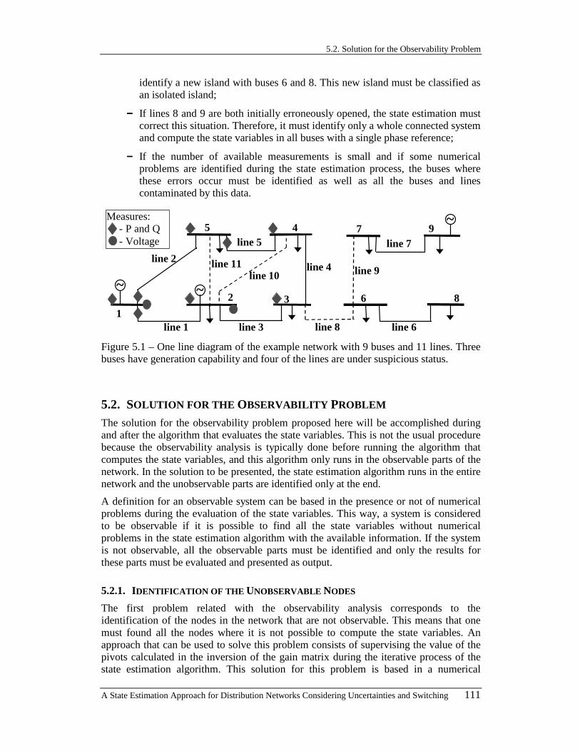
5.2. Solution for the Observability Problem
A State Estimation Approach for Distribution Networks Considering Uncertainties and Switching 111
identify a new island with buses 6 and 8. This new island must be classified as an isolated island;
−−−− If lines 8 and 9 are both initially erroneously opened, the state estimation must correct this situation. Therefore, it must identify only a whole connected system and compute the state variables in all buses with a single phase reference;
−−−− If the number of available measurements is small and if some numerical problems are identified during the state estimation process, the buses where these errors occur must be identified as well as all the buses and lines contaminated by this data.
1
~
5 4
32~
line 1 line 3
line 2line 4
line 10line 11
line 57 9
6 8
~
line 6
line 9
line 7
line 8
Measures:- P and Q- Voltage
Figure 5.1 – One line diagram of the example network with 9 buses and 11 lines. Three buses have generation capability and four of the lines are under suspicious status.
5.2. SOLUTION FOR THE OBSERVABILITY PROBLEM The solution for the observability problem proposed here will be accomplished during and after the algorithm that evaluates the state variables. This is not the usual procedure because the observability analysis is typically done before running the algorithm that computes the state variables, and this algorithm only runs in the observable parts of the network. In the solution to be presented, the state estimation algorithm runs in the entire network and the unobservable parts are identified only at the end.
A definition for an observable system can be based in the presence or not of numerical problems during the evaluation of the state variables. This way, a system is considered to be observable if it is possible to find all the state variables without numerical problems in the state estimation algorithm with the available information. If the system is not observable, all the observable parts must be identified and only the results for these parts must be evaluated and presented as output.
5.2.1. IDENTIFICATION OF THE UNOBSERVABLE NODES
The first problem related with the observability analysis corresponds to the identification of the nodes in the network that are not observable. This means that one must found all the nodes where it is not possible to compute the state variables. An approach that can be used to solve this problem consists of supervising the value of the pivots calculated in the inversion of the gain matrix during the iterative process of the state estimation algorithm. This solution for this problem is based in a numerical

Chapter 5. Observability and Splitting Problems
112 A State Estimation Approach for Distribution Networks Considering Uncertainties and Switching
analysis procedure that corresponds to one type of observability analysis. As it was referred in Chapter 2, this type of analysis is based on the analysis of the matrices of the state estimation algorithm. These matrices can be the gain matrix or a factorization of the gain matrix.
To solve this problem, in the state estimation algorithm it must also be included additional instructions to check the presence or not of zero pivots in the factorization or in the process used to invert the gain matrix. When a zero pivot is founded the associated state variable is marked as unobservable and the inverse of this pivot is set to zero. The state variable that is marked with unobservable status, is, from this moment onwards, with this status until the end of the state estimation algorithm. This means that, even if this pivot gets different from zero, in the next iterations, the inverse of this pivot is always zero because the state variable has been unobservable in a previous iteration.
The action of putting the value of the inverse of a zero pivot equal to zero means that the respective state variable will be assigned a zero value. In this way, the state variables marked with the unobservable status have the zero value as result and these zero values can affect some nearby buses if the number of measurements available for these buses is small.
The instructions that must be added to prevent possible numerical errors during the state estimation algorithm, caused by the observability problem, are described in the following paragraphs.
Modified State Estimation Algorithm
−−−− Initially mark all state variables with the observable status;
−−−− (…)
−−−− In each iteration of the state estimation algorithm, in the factorization process:
■ If the current column number is associated to a unobservable state variable, set the pivot inverse equal to zero;
■ Else if the pivot of this column number is zero, mark the state variable with the unobservable status and set the pivot inverse equal to zero;
■ Else for this column evaluate the factorization using the usual procedure;
−−−− (…)
For instance, in the example presented in Figure 5.1 the state estimation algorithm always runs in the entire network, independently of the number and the position of the available measurements and pseudo-measurements. This means that, from the state estimation problem point of view, this network has always 9 buses and 11 lines. However, during the algorithm, the unobservable state variables are identified and, as result, these variables have zero values. Nevertheless, at the end of the algorithm it is also needed to identify all the equipments affected by the non observability of these state variables. This corresponds to another problem that is addressed in the next section.

5.2. Solution for the Observability Problem
A State Estimation Approach for Distribution Networks Considering Uncertainties and Switching 113
5.2.2. IDENTIFICATION OF THE UNOBSERVABLE EQUIPMENTS
The second problem related with the observability analysis is the identification of all the equipments on the system where the values obtained by the state estimation algorithm can be affected by the nodes that are unobservable. The results obtained for these equipments can be meaningless because the zero values of the unobservable state variables can influence the state variables marked with observable status in the nearby buses.
The algorithm adopted to solve this problem is based in two facts. The first fact is that a branch that connects two unobservable buses is also unobservable. The second fact is that an unobservable bus that is connected to another bus without measurements by a branch also without measurements, is an unobservable bus. In that case, the branch that makes the connection is also unobservable. A bus is considered with valid measurements if it has measurements of active and reactive power injections or active power injection and voltage magnitude. Moreover, the branch is considered with valid measurements if it has measurements of active and reactive power flow, or a current magnitude with a power factor value. In the last case, it must be also available information about the inductive or capacitive nature of the referred current.
When the state estimation algorithm ends, one has the values for the state variables. The next step corresponds to the identification of the observable buses and branches. To carry on this analysis, the branches between unobservable buses are also unobservable but they have to be considered to complete the observability analysis. This means that, a branch and the related buses must be analyzed by the observability algorithm if that branch has an opened result from the state estimation run and one of its terminals is unobservable. This way, if the conclusion of this algorithm is in such that the branch is unobservable, the state estimation result for the status of that branch must be ignored.
The algorithm that marks the buses and the branches in the system with observable or unobservable status is described in the following paragraphs. The other equipments in the network are observable if their terminal buses are observable or, on the other hand, they are unobservable if their terminal buses are unobservable.
Finding All Unobservable Buses and Branches
−−−− If all state variables are marked with observable status then set all branches and all buses with observable status and exit from this procedure;
−−−− For each bus i in the system:
■ If bus i has at least one state variable unobservable, then set this bus with unobservable status and keep it in the array of buses to visit;
■ Else set bus i with observable status;
−−−− Mark all branches with observable status;
−−−− For each bus i in the array of buses to visit:
■ For each bus j connected to bus i by branch k:
• If bus j is marked with unobservable status then mark branch k with unobservable status;

Chapter 5. Observability and Splitting Problems
114 A State Estimation Approach for Distribution Networks Considering Uncertainties and Switching
• Else if branch k and bus j do not have a pair of valid measurements then put bus j in the array of buses to visit and mark bus j and branch k with unobservable status;
−−−− End of the algorithm.
5.2.3. IDENTIFICATION OF THE STATUS OF THE ISLANDS
The third problem related with the observability analysis corresponds to the identification of the different sub-systems that can be energized or isolated. This problem only exists when the state estimation algorithm founds the topology in operation, and in the input data are included some switching devices whose statuses are suspicious or even unknown.
After solving the two previous problems, the solution for this problem is easier to find. The classification of islands only makes sense if in the island exists at least one observable bus and the branches with suspicious or unknown status at the beginning have, at the end, its status identified and are observable. Otherwise, the number of islands and their identification can be affected since the topology is not completely identified.
An island is classified as energized if in the set of buses in the island there is, at least, one bus with generation capability. This bus can have a generator or a connection to a network of other voltage level. This means that all loads in this island are supplied, but it may not be possible to compute the values of all variables. Obviously, this computation is possible if the island is observable in terms of all buses and branches.
An island is classified as isolated if in the set of buses in that island there isn’t any bus with generation capability. This means that the loads in this island are not supplied. In this case, the computation of all variables is possible even if the island is not observable in terms of all buses and branches, because the values for the voltages, powers and currents are all zero.
When a branch with suspicious or unknown status at the beginning of the state estimation algorithm has, at the end, an unobservable status, this result must be discarded. In fact, one has to consider the two possibilities of status, opened or closed, in order to identify the possible resulting topologies. Furthermore, for each status it is important to provide as output the number of islands that are identified and the respective status.
5.2.4. ILLUSTRATIVE EXAMPLE
We will now present an example of application of this algorithm, based on the network presented in Figure 5.1. In this network, the state estimation algorithm runs in the entire network considering that the measurements used are represented in Figure 5.1 and considering that the suspicious lines are all closed. The algorithm identifies the correct topology for the lines where this is possible (lines 8, 10 and 11). However, during the algorithm, the unobservable identified state variables are the voltage magnitudes and the voltage phases in buses 7, 8 and 9. Applying the described algorithm to this example we can consider the following steps:
Example of Algorithm Run

5.2. Solution for the Observability Problem
A State Estimation Approach for Distribution Networks Considering Uncertainties and Switching 115
−−−− bus 7 is marked with unobservable status and it is kept in the array to visit;
−−−− bus 8 is marked with unobservable status and it is kept in the array to visit;
−−−− bus 9 is marked with unobservable status and it is kept in the array to visit;
−−−− all other buses (from 1 to 6) are marked with observable status;
−−−− all branches are marked with observable status;
−−−− set i= 7; ■ set j=6;
• bus 6 is kept in the array to visit and bus 6 and line 9 are marked with unobservable status;
■ set j=9; • line 7 is marked with unobservable status;
−−−− set i= 8; ■ set j=6;
• line 6 is marked with unobservable status;
−−−− set i=9; ■ set j=7;
• line 7 is marked with unobservable status;
−−−− set i=6; ■ set j=3;
• do nothing because bus 3 has a pair of valid measurements; ■ set j=7;
• line 9 is marked with unobservable status; ■ set j=8;
• line 6 is marked with unobservable status;
For this example, the results of the observability analysis are:
−−−− buses from 1 to 5 are observable;
−−−− buses from 6 to 9 are unobservable;
−−−− lines 1, 2, 3, 4, 5, 8, 10 and 11 are observable;
−−−− lines 6, 7 and 9 are unobservable.
In this example, line 9 has at beginning a suspicious status and, at the end, is unobservable. This means, that the two possible statuses for line 9 must be considered as equally possible. If line 9 is opened, the system integrates two islands that are both energized, because one has the generation buses 1 and 2, and the other has the generation bus 9. On the other hand, if line 9 is closed, the system is composed by a single island having three generation buses.

Chapter 5. Observability and Splitting Problems
116 A State Estimation Approach for Distribution Networks Considering Uncertainties and Switching
5.3. SOLUTION FOR THE SPLITTING PROBLEM
5.3.1. FORMULATION
The consideration of uncertainty affecting topology variables introduces in the state estimation problem a new focusing that one denotes as the Splitting Problem. A way to treat the problem of system splitting that will be detailed in this section, was firstly presented in references [4] and [5].
In fact, traditional state estimation approaches assume that the topology is known and that is fixed a priori. Therefore, it is assumed that the whole system corresponds to an unique connected island, or a well pre-defined number of islands. In this case, there is no splitting problem, because the number of islands at the beginning and at the end of the state estimation process is always the same.
Admitting uncertainties regarding the statuses of switching devices implies that one should also admit that the system currently in operation is initially considered as a single island but may in fact integrate a set of non-connected islands. Another situations that can occur are related with the number of islands at the beginning and at the end of the state estimation. On one hand, the number of islands admitted for the system can be smaller than the number of islands really existing on the system. On the other hand, it can occur that the number of islands admitted for the system can be larger than the number of islands really existent on the system. In this situation, even a system admitted as non-connected can result in a single island at the end of the state estimation process.
In some of these situations, from a state estimation point of view, this is a very appealing possibility since the available measurements can be more adequately explained by a different topology than the initially considered as input. On one hand, it can happen that this explanation can be more adequate for a non-connected system while the system is initially considered as connected. On the other hand, the measurements can be more adequately explained for a connected system while the system is initially considered as non-connected. This means that the sum of the squares of the errors of the measurements can be smaller if one admits a different topology with a different number of islands when compared to the values of the initial topology for the system.
In other words, incorporating these situations in the state estimation contributes to increase the flexibility of the model and definitely contributes to model real systems in a more adequate way. In traditional formulations splitting of the system was not possible since there was an unique bus selected for reference of the phases in each considered island. For instance, let us consider again the problem that is represented in Figure 5.1 and let us suppose that the suspicious lines are initially considered closed. In the beginning, all the combinations of open/close for each of these lines are possible. The solution that fits in the best way to the measurements is the one that is selected by the state estimation algorithm.
In the state estimation algorithm described in this Thesis, the number of islands at the beginning of the algorithm can be different from the number of islands at the end. If in the state estimation algorithm it is used the traditional way to fix the voltage phases in some buses, there will be some problems. In this case, if the splitting in one or more islands occurs some matrices would be singular introducing numerical problems in the state estimation process and consequently compromising the solution of the state
5.3. Solution for the Splitting Problem
A State Estimation Approach for Distribution Networks Considering Uncertainties and Switching 117
estimation problem. On the other hand, if a splitting is initially considered in some islands and at the end there is only one island, the solution is affected by the existence of several buses in the same island having fixed voltage. This situation also compromises the solution of the state estimation problem.
This difficulty can be solved if, instead of fixing a voltage phase in a bus for each island, one associates to each node with generation capability a voltage phase pseudo--measurement, having the zero value initially assigned. These nodes are selected for the reason that for an island to be in operation it must have at least one node with generation to supply the loads in the island. If in one identified island there are no nodes with generation, the results must be discarded because the island is classified as isolated. In this case, if there are loads included on it, then they are not supplied.
The association of a phase value for each node with generation capability is accomplished by including in the model a pseudo-measurement for these voltage phases. This pseudo-measurement has a zero value and it is represented using expression (5.1). In this expression, the variable iθ represents the voltage phase in node
i, which is a state variable, the variable iθε represents the voltage angle measurement
error and i represents the index of one node having generation capability.
ii0 θεθ += (5.1)
Since one does not know how many islands there are in the system, or even if the system is actually splitted or not, a large weight is assigned to the voltage phase measurement in one of these nodes. This node is the one that has the largest generation connected to it. The reason for selecting this node is that in general, this would be the reference for the whole system when it was completely connected and when there is only a single energized island. The inclusion of pseudo-measurements for all possible references in the entire system, including in this node, means that the number of voltage phases in the state vector is the same of the number of voltage magnitudes in this vector. In this case, all the voltage phases are considered state variables. In the traditional formulation, the number of state variables corresponding to voltage phases, is given by the number of nodes minus the number of phase references that are considered, because in this case these fixed voltage phases are not state variables.
The weights of the remaining voltage phase pseudo-measurements should be smaller. In the algorithm, these pseudo-measurements have the effect of being used only if necessary. If they are not necessary, they do not affect the results of the state estimation algorithm. This does not compromise any of the two possible ways of operation of the system:
−−−− If the operation in an unique island is the more adequate one, from the state estimation point of view, the estimated phase for the larger generation node will be zero. The pseudo-measurement values of voltage phases in the remaining generation nodes are affected by errors. However, the corresponding residuals will not determine in a significant way the final state vector since their weights are very small;

Chapter 5. Observability and Splitting Problems
118 A State Estimation Approach for Distribution Networks Considering Uncertainties and Switching
−−−− On the other hand, if splitting the system in islands is the most convenient situation, one has the possibility of obtaining a zero phase reference in each island if at least one generation node exists in each of them.
The splitting problem for the energized parts of the network is solved. There is now a new problem that emerges from the previous analysis. This problem occurs when an island is isolated and there is no reference for the phases included on it. These islands have other problems related with the other measurements affected by errors and, in general, these parts of the network are unobservable. These problems were discussed in section 5.2.3 of this thesis.
5.3.2. ILLUSTRATIVE EXAMPLE
In the problem illustrated with the system in Figure 5.1 there are three nodes with generation capability, node 1, node 2 and node 9. In this way, three zero pseudo--measurements are included in the model and we use equations represented by (5.2) for the node 1, (5.3) for the node 2 and (5.4) for the node 9. Let us consider that node 1 has the largest generation. In this case, a larger weight is associated to the zero pseudo--measurement related to (5.2), and smaller weights will be assigned to the other two pseudo-measurements.
110 θεθ += (5.2)
220 θεθ += (5.3)
990 θεθ += (5.4)
In this example, at the end of the state estimation algorithm the state variable voltage phase in node 1 will be zero and it is the reference for phases in the island. The voltage phase in node 2 will be evaluated by the other available measurements and its zero value in the pseudo-measurement has an error associated to it. Finally, the voltage phase in node 9 will be zero if line 8 or line 9 are opened, or it is evaluated using the other measurements if these lines are closed.
The number of state variables in the network used in this Chapter is always 22, because the number of buses is 9 and it is considered that 4 lines have suspicious status. For each node in the network it is always considered two state variables, one voltage magnitude and one voltage phase, even if the node is the island phase reference.
5.4. ILLUSTRATIVE EXAMPLES
5.4.1. CASE 1 - TWO ENERGIZED ISLANDS
The first example is based in the system of Figure 5.1 admitting that line 9 is considered initially erroneously closed. If the state estimation algorithm has enough information, it must correct this situation by identifying a new energized island with buses 7 and 9. The other suspicious lines statuses have the correct values as opened for lines 10 and 11 and closed for line 8.
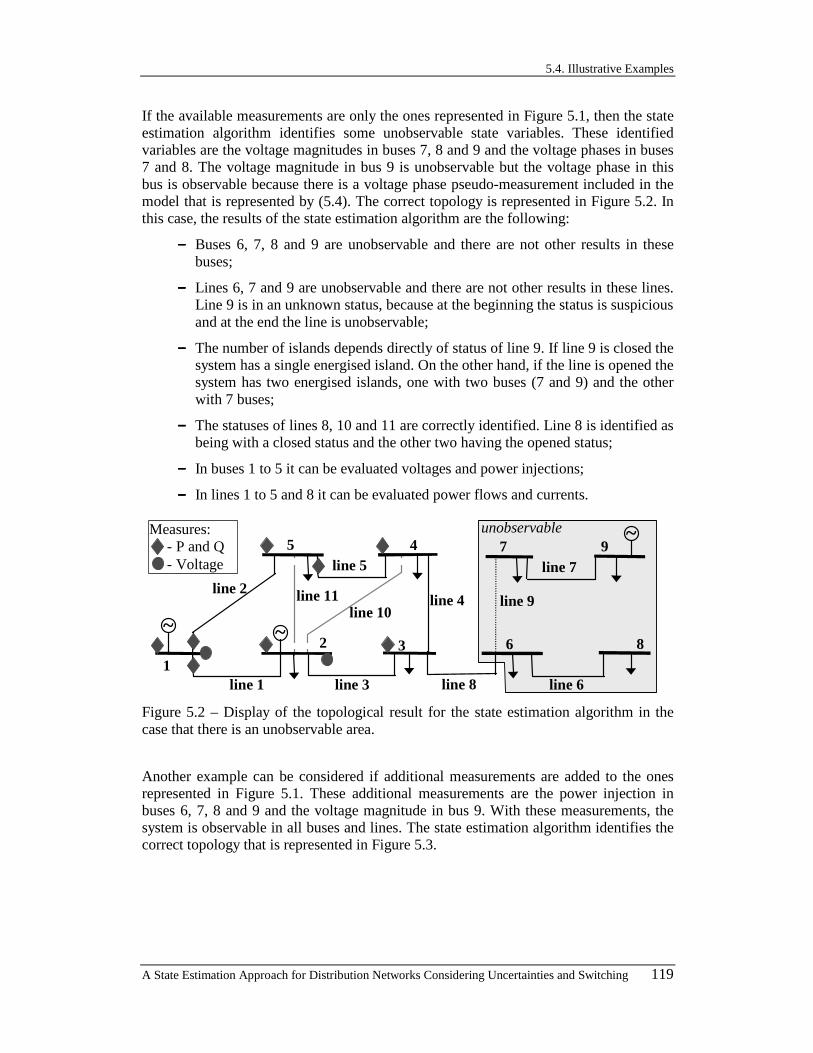
5.4. Illustrative Examples
A State Estimation Approach for Distribution Networks Considering Uncertainties and Switching 119
If the available measurements are only the ones represented in Figure 5.1, then the state estimation algorithm identifies some unobservable state variables. These identified variables are the voltage magnitudes in buses 7, 8 and 9 and the voltage phases in buses 7 and 8. The voltage magnitude in bus 9 is unobservable but the voltage phase in this bus is observable because there is a voltage phase pseudo-measurement included in the model that is represented by (5.4). The correct topology is represented in Figure 5.2. In this case, the results of the state estimation algorithm are the following:
−−−− Buses 6, 7, 8 and 9 are unobservable and there are not other results in these buses;
−−−− Lines 6, 7 and 9 are unobservable and there are not other results in these lines. Line 9 is in an unknown status, because at the beginning the status is suspicious and at the end the line is unobservable;
−−−− The number of islands depends directly of status of line 9. If line 9 is closed the system has a single energised island. On the other hand, if the line is opened the system has two energised islands, one with two buses (7 and 9) and the other with 7 buses;
−−−− The statuses of lines 8, 10 and 11 are correctly identified. Line 8 is identified as being with a closed status and the other two having the opened status;
−−−− In buses 1 to 5 it can be evaluated voltages and power injections;
−−−− In lines 1 to 5 and 8 it can be evaluated power flows and currents.
1
~
5 4
32~
line 1 line 3
line 2line 4
line 57 9
6 8
~
line 6
line 7
line 8
Measures:- P and Q- Voltage
line 9
unobservable
line 10line 11
Figure 5.2 – Display of the topological result for the state estimation algorithm in the case that there is an unobservable area.
Another example can be considered if additional measurements are added to the ones represented in Figure 5.1. These additional measurements are the power injection in buses 6, 7, 8 and 9 and the voltage magnitude in bus 9. With these measurements, the system is observable in all buses and lines. The state estimation algorithm identifies the correct topology that is represented in Figure 5.3.

Chapter 5. Observability and Splitting Problems
120 A State Estimation Approach for Distribution Networks Considering Uncertainties and Switching
1
~
5 4
32~
line 1 line 3
line 2line 4
line 57 9
6 8
~
line 6
line 7
line 8
Measures:- P and Q- Voltage
line 9line 10
line 11
Figure 5.3 – Display of the topological result for the state estimation algorithm in the case there are two energized islands.
In this case, the state estimation algorithm identifies two energized islands. The occurred splitting has no problems related with the need of two distinct phase references at the end of the algorithm when at the beginning it is required only one phase reference. This happens because the status of line 9 is erroneously closed at the beginning, and this situation is corrected by the algorithm. If the three pseudo-measurements for the voltage phase are not considered and it is fixed only the phase reference on the bus 1, at the end of the state estimation algorithm there is a state variable that is unobservable. This variable is one voltage phase in the energized island that includes buses 7 and 9.
The values for the phase voltages pseudo-measurements considered at buses 1 and 9 are used. This means that the results for the phase in these buses are the value 0.0. On the other hand, the pseudo-measurement in bus 2 is not used and the result for the phase in this bus is -0.00042 p.u.. If this pseudo-measurement were not considered the result provided by the state estimation algorithm would be the same.
5.4.2. CASE 2 - TWO ENERGIZED ISLANDS AND ONE ISOLATED ISLAND
The second example is based in the system of Figure 5.1 where lines 8 and 9 are considered initially erroneously closed. Therefore, if the state estimation algorithm has enough information, it must correct this situation by identifying an energized island with buses 7 and 9 and an isolated island with buses 6 and 8. For the other suspicious lines the algorithm assign the correct values for the state variables as opened for line 10 and closed for line 11.
If the available measurements are only the represented in Figure 5.1, as in the previous example the state estimation algorithm identifies some unobservable state variables. In this case, the identification of islands also depends on the status of line 9 that is unobservable.
We will now considered the additional measurements that were added in the second example of the previous section. This means that the measurements added are the power injection in buses 6, 7, 8 and 9 and the voltage magnitude in bus 9. With these measurements, the system is observable in all state variables with exception of the voltage phase in bus 6 (or in bus 8). The state estimation algorithm identifies the correct topology that is represented in Figure 5.4.
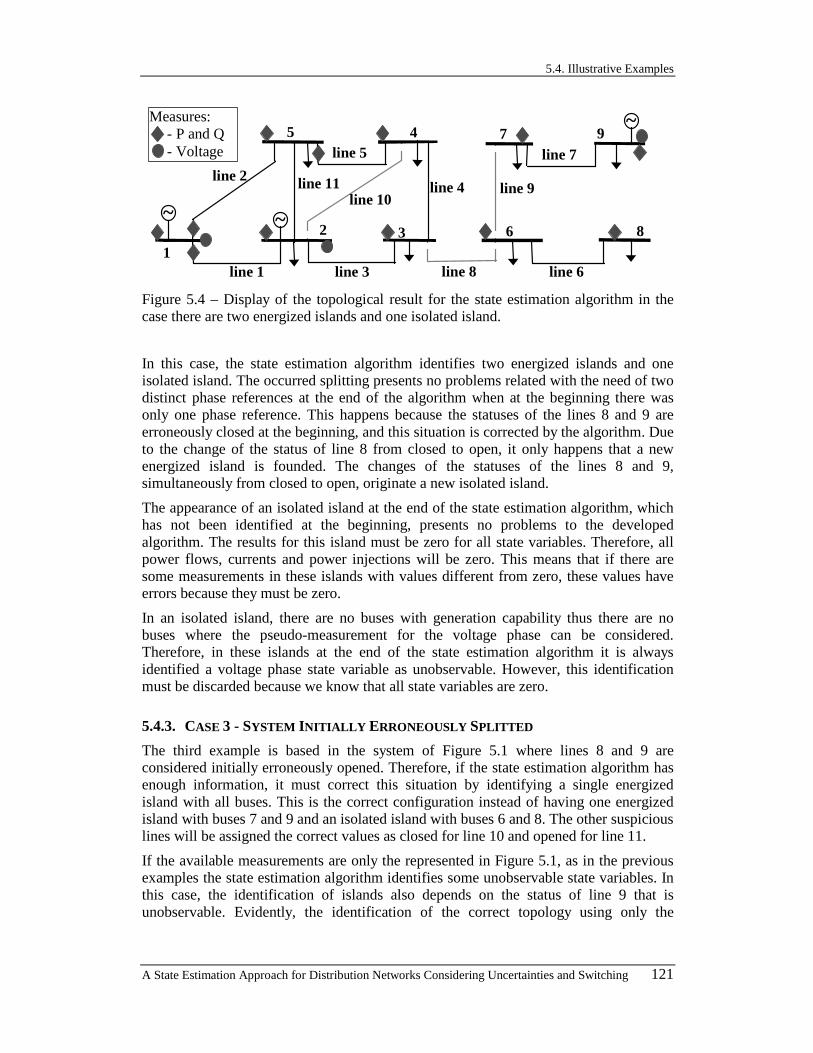
5.4. Illustrative Examples
A State Estimation Approach for Distribution Networks Considering Uncertainties and Switching 121
1
~
5 4
32~
line 1 line 3
line 2line 4
line 57 9
6 8
~
line 6
line 7
Measures:- P and Q- Voltage
line 11
line 8
line 9line 10
Figure 5.4 – Display of the topological result for the state estimation algorithm in the case there are two energized islands and one isolated island.
In this case, the state estimation algorithm identifies two energized islands and one isolated island. The occurred splitting presents no problems related with the need of two distinct phase references at the end of the algorithm when at the beginning there was only one phase reference. This happens because the statuses of the lines 8 and 9 are erroneously closed at the beginning, and this situation is corrected by the algorithm. Due to the change of the status of line 8 from closed to open, it only happens that a new energized island is founded. The changes of the statuses of the lines 8 and 9, simultaneously from closed to open, originate a new isolated island.
The appearance of an isolated island at the end of the state estimation algorithm, which has not been identified at the beginning, presents no problems to the developed algorithm. The results for this island must be zero for all state variables. Therefore, all power flows, currents and power injections will be zero. This means that if there are some measurements in these islands with values different from zero, these values have errors because they must be zero.
In an isolated island, there are no buses with generation capability thus there are no buses where the pseudo-measurement for the voltage phase can be considered. Therefore, in these islands at the end of the state estimation algorithm it is always identified a voltage phase state variable as unobservable. However, this identification must be discarded because we know that all state variables are zero.
5.4.3. CASE 3 - SYSTEM INITIALLY ERRONEOUSLY SPLITTED
The third example is based in the system of Figure 5.1 where lines 8 and 9 are considered initially erroneously opened. Therefore, if the state estimation algorithm has enough information, it must correct this situation by identifying a single energized island with all buses. This is the correct configuration instead of having one energized island with buses 7 and 9 and an isolated island with buses 6 and 8. The other suspicious lines will be assigned the correct values as closed for line 10 and opened for line 11.
If the available measurements are only the represented in Figure 5.1, as in the previous examples the state estimation algorithm identifies some unobservable state variables. In this case, the identification of islands also depends on the status of line 9 that is unobservable. Evidently, the identification of the correct topology using only the

Chapter 5. Observability and Splitting Problems
122 A State Estimation Approach for Distribution Networks Considering Uncertainties and Switching
referred measurements is very difficult and the algorithm can lead to some errors, specially in the identification of the closed status of line 8.
We will now consider this example with the additional measurements that were added in the two previous examples in the previous section. This means that the measurements added are the power injection in buses 6, 7, 8 and 9 and the voltage magnitude in bus 9. With these measurements, the system is observable in all buses and all lines. The state estimation algorithm identifies the correct topology that is represented in Figure 5.5.
In this case, the state estimation algorithm identifies a single energized island, while the input data indicates that the system has two energized islands and one isolated island. The initially wrong splitting poses no problems related with the inclusion of only one phase reference at the end of the algorithm when, at the beginning, they were required two phase references. This happens because the statuses of lines 8 and 9 are erroneously opened at the beginning, and this situation is corrected by the algorithm. By changing the status of line 9 from opened to close, it only happens that the isolated island is eliminated. However, changing the statuses of lines 8 and 9 simultaneously from opened to close, leads to the connection of the two initially energized islands thus creating a single one.
With the algorithm described, the number of phase references can be different in the beginning and at the end of the state estimation algorithm. In this case, there are three pseudo-measurements for the voltage phases, which were considered at the beginning. At the end of the state estimation algorithm, it is fixed only the phase reference at bus 1. The voltage phase state variable in bus 9 is evaluated by the algorithm. Moreover, the value fixed at the beginning using the pseudo-measurement (5.4) is ignored and an error will be associated to this measurement. This error has no effect in the other measurements because the weight that is related with this value is small.
1
~
5 4
32~
line 1 line 3
line 2line 4
line 57 9
6 8
~
line 6
line 7
line 8
Measures:- P and Q- Voltage
line 10 line 9line 11
Figure 5.5 – Display of the example network result from the state estimation algorithm and with a single island including the 11 nodes.
As for the voltage phase pseudo-measurement in bus 9, it also occurs that the voltage phase pseudo-measurement in bus 2 is not used. This means that the results for the phase in buses 2 and 9 are evaluated by the state estimator algorithm. The result for the voltage phase in bus 2 is -0.00378 p.u. and in bus 9 is -0.04843 p.u.. If the referred phase pseudo-measurements for these two nodes were not used, the state estimation algorithm would provide the same values for the estimates phases in buses 2 and 9.

5.5. Chapter References
A State Estimation Approach for Distribution Networks Considering Uncertainties and Switching 123
5.5. CHAPTER REFERENCES
[1] Y. M. Park, Y. H. Moon, J. B. Choo, T. W. Kwon, “Design of Reliable Measurement System for State Estimation”, IEEE Transactions on Power Systems, Vol. 3, No. 3, pp. 830-836, Aug. 1988.
[2] G. N. Korres, G. C. Contaxis, “Identification and Updating of Minimally Dependent Sets of Measurements in State Estimation”, IEEE Transactions on Power Systems, Vol. 6, No. 3, pp. 999-1005, Aug. 1991.
[3] A. Abur, F. H. Magnago, “Optimal Meter Placement for Maintaining Observability During Single Branch Outages”, IEEE Transactions on Power Systems, Vol. 14, No. 4, pp. 1273-1278, Nov. 1999.
[4] J. Pereira, J. T. Saraiva, V. Miranda, “A Comprehensive State Estimation Approach for EMS/DMS Applications”, Proceedings of IEEE Budapest Power Tech´99, paper BPT99-358-16, Budapest, Hungary, Aug. 1999.
[5] J. Pereira, J. T. Saraiva, V. Miranda, “Estimação de Estado em Sistemas de Distribuição de Energia Incluindo Aparelhos de Corte, Divisão em Ilhas e Dados Qualitativos”, Revista Eletroevolução, CIGRÉ - Brasil, No. 16, pp. 69-75, Jun. 1999.

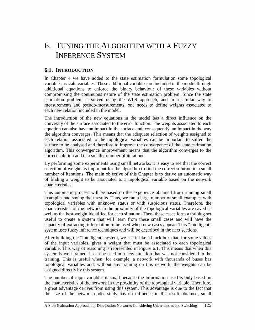
A State Estimation Approach for Distribution Networks Considering Uncertainties and Switching 125
6. TUNING THE ALGORITHM WITH A FUZZY INFERENCE SYSTEM
6.1. INTRODUCTION In Chapter 4 we have added to the state estimation formulation some topological variables as state variables. These additional variables are included in the model through additional equations to enforce the binary behaviour of these variables without compromising the continuous nature of the state estimation problem. Since the state estimation problem is solved using the WLS approach, and in a similar way to measurements and pseudo-measurements, one needs to define weights associated to each new relation included in the model.
The introduction of the new equations in the model has a direct influence on the convexity of the surface associated to the error function. The weights associated to each equation can also have an impact in the surface and, consequently, an impact in the way the algorithm converges. This means that the adequate selection of weights assigned to each relation associated to the topological variables can be important to soften the surface to be analysed and therefore to improve the convergence of the state estimation algorithm. This convergence improvement means that the algorithm converges to the correct solution and in a smaller number of iterations.
By performing some experiments using small networks, it is easy to see that the correct selection of weights is important for the algorithm to find the correct solution in a small number of iterations. The main objective of this Chapter is to derive an automatic way of finding a weight to be associated to a topological variable based on the network characteristics.
This automatic process will be based on the experience obtained from running small examples and saving their results. Thus, we ran a large number of small examples with topological variables with unknown status or with suspicious status. Therefore, the characteristics of the network in the proximity of the topological variables are saved as well as the best weight identified for each situation. Then, these cases form a training set useful to create a system that will learn from these small cases and will have the capacity of extracting information to be used when new cases appear. This “intelligent” system uses fuzzy inference techniques and will be described in the next sections.
After building the “intelligent” system, we use it like a black box that, for some values of the input variables, gives a weight that must be associated to each topological variable. This way of reasoning is represented in Figure 6.1. This means that when this system is well trained, it can be used in a new situation that was not considered in the training. This is useful when, for example, a network with thousands of buses has topological variables and, without any training on this network, the weights can be assigned directly by this system.
The number of input variables is small because the information used is only based on the characteristics of the network in the proximity of the topological variable. Therefore, a great advantage derives from using this system. This advantage is due to the fact that the size of the network under study has no influence in the result obtained, small
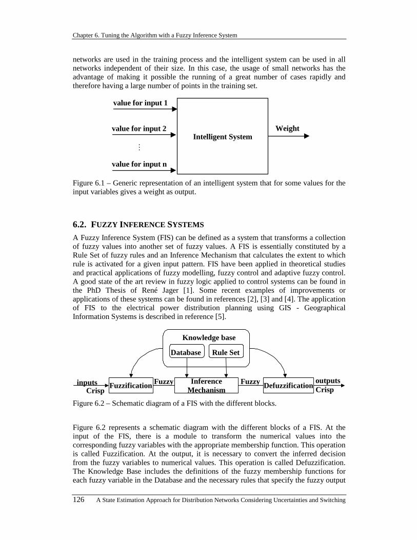
Chapter 6. Tuning the Algorithm with a Fuzzy Inference System
126 A State Estimation Approach for Distribution Networks Considering Uncertainties and Switching
networks are used in the training process and the intelligent system can be used in all networks independent of their size. In this case, the usage of small networks has the advantage of making it possible the running of a great number of cases rapidly and therefore having a large number of points in the training set.
Intelligent SystemWeight
value for input 1
value for input 2
value for input n
M
Figure 6.1 – Generic representation of an intelligent system that for some values for the input variables gives a weight as output.
6.2. FUZZY INFERENCE SYSTEMS A Fuzzy Inference System (FIS) can be defined as a system that transforms a collection of fuzzy values into another set of fuzzy values. A FIS is essentially constituted by a Rule Set of fuzzy rules and an Inference Mechanism that calculates the extent to which rule is activated for a given input pattern. FIS have been applied in theoretical studies and practical applications of fuzzy modelling, fuzzy control and adaptive fuzzy control. A good state of the art review in fuzzy logic applied to control systems can be found in the PhD Thesis of René Jager [1]. Some recent examples of improvements or applications of these systems can be found in references [2], [3] and [4]. The application of FIS to the electrical power distribution planning using GIS - Geographical Information Systems is described in reference [5].
Fuzzification InferenceMechanism
Defuzzificationinputs outputsFuzzy
Knowledge base
Database Rule Set
FuzzyCrisp Crisp
Figure 6.2 – Schematic diagram of a FIS with the different blocks.
Figure 6.2 represents a schematic diagram with the different blocks of a FIS. At the input of the FIS, there is a module to transform the numerical values into the corresponding fuzzy variables with the appropriate membership function. This operation is called Fuzzification. At the output, it is necessary to convert the inferred decision from the fuzzy variables to numerical values. This operation is called Defuzzification. The Knowledge Base includes the definitions of the fuzzy membership functions for each fuzzy variable in the Database and the necessary rules that specify the fuzzy output
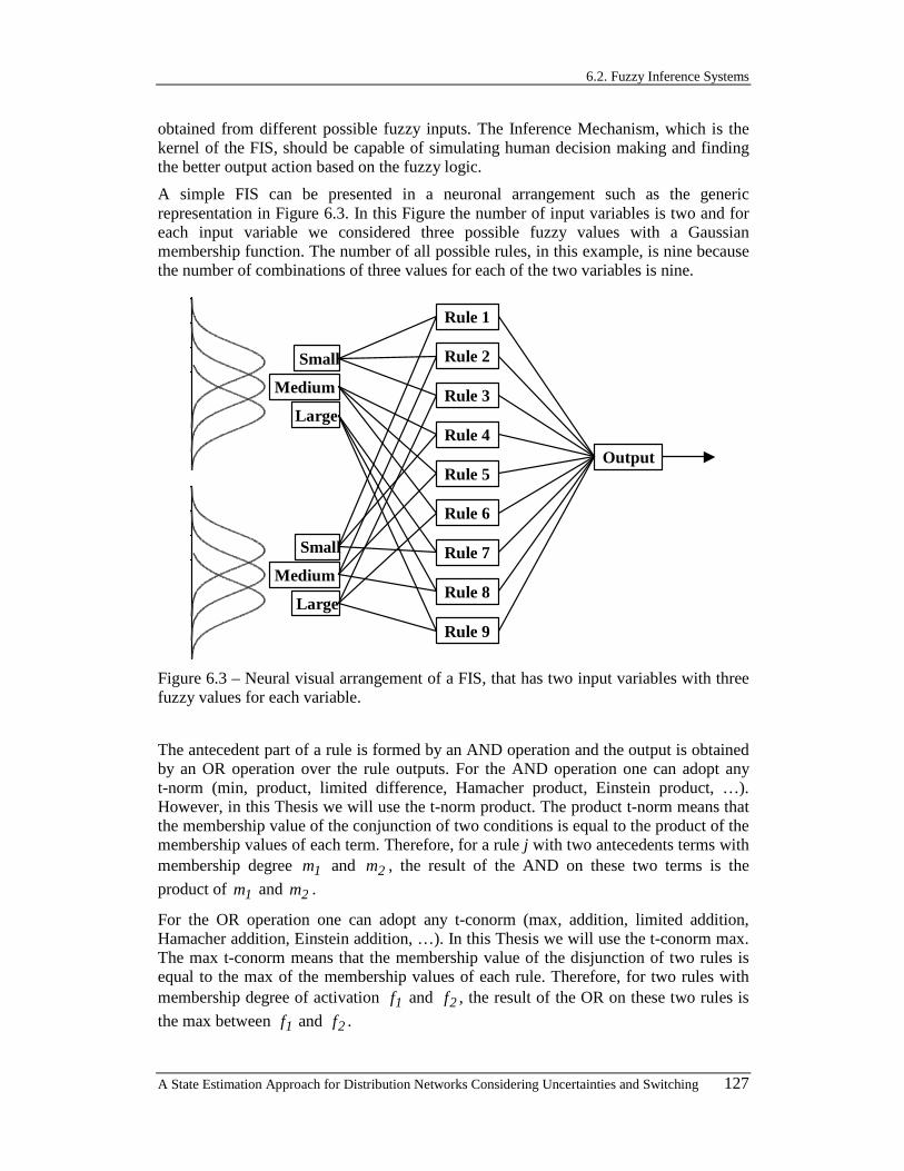
6.2. Fuzzy Inference Systems
A State Estimation Approach for Distribution Networks Considering Uncertainties and Switching 127
obtained from different possible fuzzy inputs. The Inference Mechanism, which is the kernel of the FIS, should be capable of simulating human decision making and finding the better output action based on the fuzzy logic.
A simple FIS can be presented in a neuronal arrangement such as the generic representation in Figure 6.3. In this Figure the number of input variables is two and for each input variable we considered three possible fuzzy values with a Gaussian membership function. The number of all possible rules, in this example, is nine because the number of combinations of three values for each of the two variables is nine.
Small
Medium
Large
Small
Medium
Large
Rule 1
Output
Rule 2
Rule 3
Rule 4
Rule 5
Rule 6
Rule 7
Rule 8
Rule 9
Figure 6.3 – Neural visual arrangement of a FIS, that has two input variables with three fuzzy values for each variable.
The antecedent part of a rule is formed by an AND operation and the output is obtained by an OR operation over the rule outputs. For the AND operation one can adopt any t-norm (min, product, limited difference, Hamacher product, Einstein product, …). However, in this Thesis we will use the t-norm product. The product t-norm means that the membership value of the conjunction of two conditions is equal to the product of the membership values of each term. Therefore, for a rule j with two antecedents terms with membership degree 1m and 2m , the result of the AND on these two terms is the
product of 1m and 2m .
For the OR operation one can adopt any t-conorm (max, addition, limited addition, Hamacher addition, Einstein addition, …). In this Thesis we will use the t-conorm max. The max t-conorm means that the membership value of the disjunction of two rules is equal to the max of the membership values of each rule. Therefore, for two rules with membership degree of activation 1f and 2f , the result of the OR on these two rules is
the max between 1f and 2f .
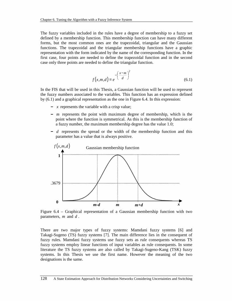
Chapter 6. Tuning the Algorithm with a Fuzzy Inference System
128 A State Estimation Approach for Distribution Networks Considering Uncertainties and Switching
The fuzzy variables included in the rules have a degree of membership to a fuzzy set defined by a membership function. This membership function can have many different forms, but the most common ones are the trapezoidal, triangular and the Gaussian functions. The trapezoidal and the triangular membership functions have a graphic representation with the form indicated by the name of the corresponding function. In the first case, four points are needed to define the trapezoidal function and in the second case only three points are needed to define the triangular function.
( )2
d
mx
ed,m,xf
−−
= (6.1)
In the FIS that will be used in this Thesis, a Gaussian function will be used to represent the fuzzy numbers associated to the variables. This function has an expression defined by (6.1) and a graphical representation as the one in Figure 6.4. In this expression:
−−−− x represents the variable with a crisp value;
−−−− m represents the point with maximum degree of membership, which is the point where the function is symmetrical. As this is the membership function of a fuzzy number, the maximum membership degree has the value 1.0;
−−−− d represents the spread or the width of the membership function and this parameter has a value that is always positive.
0
.3679
1
m
Gaussian membership function
x
( )d,m,xf
m+dm-d Figure 6.4 – Graphical representation of a Gaussian membership function with two parameters, m and d .
There are two major types of fuzzy systems: Mamdani fuzzy systems [6] and Takagi-Sugeno (TS) fuzzy systems [7]. The main difference lies in the consequent of fuzzy rules. Mamdani fuzzy systems use fuzzy sets as rule consequents whereas TS fuzzy systems employ linear functions of input variables as rule consequents. In some literature the TS fuzzy systems are also called by Takagi-Sugeno-Kang (TSK) fuzzy systems. In this Thesis we use the first name. However the meaning of the two designations is the same.

6.2. Fuzzy Inference Systems
A State Estimation Approach for Distribution Networks Considering Uncertainties and Switching 129
An example of a generic rule for a Mamdani fuzzy system is given by (6.2). This expression represents the rule number j of a Rule Set. This rule has n input fuzzy variables ( n1 x ..., ,x ) and one output fuzzy variable (y). In this rule, the symbols that appear in it have the following meaning:
−−−− ijA represents the fuzzy number associated to the input variable ix in the rule
number j , which is characterised by the membership function ( )iij xf ;
−−−− jB represents the fuzzy number associated to the output variable y in the rule
number j , which is characterised by the membership function ( )yf j0 .
jnjnj11 y is B is Ax... is Ax THEN AND AND IF (6.2)
To define a FIS of the Mamdani type, with Gaussian membership functions and one output variable, the following parameters are required:
−−−− Number of linguistic labels for each input variable;
−−−− Number of linguistic labels for the output variable;
−−−− Values of parameters m and d for each membership function;
−−−− Defuzzification procedure. This can be the centre-of-gravity method (COG) or the mean of maximums method (MOM).
An example of one generic rule for a TS fuzzy system is given by (6.3). This expression represents the rule number j of a Rule Set. This rule has also n input fuzzy variables ( n1 x ..., ,x ) and one output variable ( jy ). In this rule, the symbols in it have the
following meaning:
−−−− ijA represents the fuzzy number associated to the input variable ix in the rule
number j , which is characterised by the membership function ( )iij xf ;
−−−− ija represents the coefficients (numerical weights) associated to each input
variable ix in the rule number j . If these values are zero for i>0 the FIS is called Zero-Order TS fuzzy system. Otherwise the FIS is called First-Order TS fuzzy system;
−−−− j0a represents the constant coefficient (numerical weight) associated to the
rule number j .
nnj1j1j0jnjnj11 xa...xaay is Ax... is Ax +++= THEN AND AND IF (6.3)
In a FIS based on a TS fuzzy system the OR operation is not needed because the output of each rule j is a crisp number jy given by the expression (6.4).

Chapter 6. Tuning the Algorithm with a Fuzzy Inference System
130 A State Estimation Approach for Distribution Networks Considering Uncertainties and Switching
∑=
+=n
1iiij0jj xaay (6.4)
The result of the inference system is obtained by the expression (6.5), which is the weighted addition of all outputs of all activated rules. In this expression, an represents
the number of rules activated by the input and jg represents the firing strength of rule
j which is evaluated using expression (6.6).
∑
∑
=
==a
a
n
1jj
n
1jjj
g
yg
y (6.5)
( ) ( ) ( )nnj2j21j1j xfxfxfg ×××= L (6.6)
To define a FIS based on the first-order TS fuzzy system with Gaussian membership functions the following parameters need to be specified:
−−−− Number of linguistic labels for each input variable;
−−−− Values of m and d for each membership function;
−−−− Weights j0a and ija for each rule j .
The great advantage of the TS model corresponds to its representing power. It is capable of describing a highly nonlinear system using a small number of rules. Moreover, since the output of the model has an explicit functional expression given by (6.5), it is conventional to identify its parameters using some learning algorithms. Several commonly used fuzzy neural systems such as adaptive neuro-fuzzy inference system (ANFIS) are described by Roger Jang in reference [8]. Another learning approach to identify the parameters is presented by Nauck and Kruse in [9] and [10] and it is designated by NEFPROX (Neuro Fuzzy Function Aproximator).
6.3. USE OF A FIS TO FIND WEIGHTS
6.3.1. GENERAL ASPECTS
In this section we will describe a FIS that, for a set of input values, will find a weight for each topological variable. To do this it is necessary to define the values to be used as input variables. The input variables will be described using Gaussian membership functions. After the definition of the input variables, the FIS will be trained, by using an ANFIS. This means that the rules, the parameters for membership functions and the coefficients for the rules (in the case that the FIS is a TS fuzzy system) are obtained using an ANFIS and a training set.
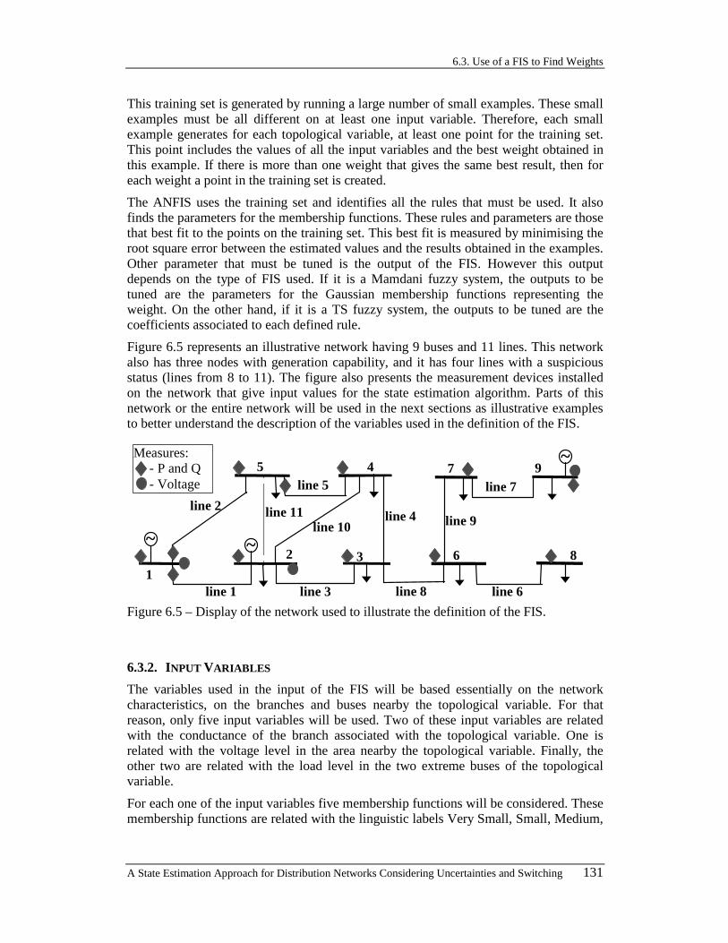
6.3. Use of a FIS to Find Weights
A State Estimation Approach for Distribution Networks Considering Uncertainties and Switching 131
This training set is generated by running a large number of small examples. These small examples must be all different on at least one input variable. Therefore, each small example generates for each topological variable, at least one point for the training set. This point includes the values of all the input variables and the best weight obtained in this example. If there is more than one weight that gives the same best result, then for each weight a point in the training set is created.
The ANFIS uses the training set and identifies all the rules that must be used. It also finds the parameters for the membership functions. These rules and parameters are those that best fit to the points on the training set. This best fit is measured by minimising the root square error between the estimated values and the results obtained in the examples. Other parameter that must be tuned is the output of the FIS. However this output depends on the type of FIS used. If it is a Mamdani fuzzy system, the outputs to be tuned are the parameters for the Gaussian membership functions representing the weight. On the other hand, if it is a TS fuzzy system, the outputs to be tuned are the coefficients associated to each defined rule.
Figure 6.5 represents an illustrative network having 9 buses and 11 lines. This network also has three nodes with generation capability, and it has four lines with a suspicious status (lines from 8 to 11). The figure also presents the measurement devices installed on the network that give input values for the state estimation algorithm. Parts of this network or the entire network will be used in the next sections as illustrative examples to better understand the description of the variables used in the definition of the FIS.
1
~
5 4
32~
line 1 line 3
line 2line 4
line 57 9
6 8
~
line 6
line 7
line 8
Measures:- P and Q- Voltage
line 10 line 9line 11
Figure 6.5 – Display of the network used to illustrate the definition of the FIS.
6.3.2. INPUT VARIABLES
The variables used in the input of the FIS will be based essentially on the network characteristics, on the branches and buses nearby the topological variable. For that reason, only five input variables will be used. Two of these input variables are related with the conductance of the branch associated with the topological variable. One is related with the voltage level in the area nearby the topological variable. Finally, the other two are related with the load level in the two extreme buses of the topological variable.
For each one of the input variables five membership functions will be considered. These membership functions are related with the linguistic labels Very Small, Small, Medium,

Chapter 6. Tuning the Algorithm with a Fuzzy Inference System
132 A State Estimation Approach for Distribution Networks Considering Uncertainties and Switching
Large and Very Large. Each one of these linguistic labels is represented by a fuzzy set that has a membership function with the following form:
−−−− The Very Small linguistic label will be associated with a Gaussian membership function given by expression (6.1) considering only values of x greater than m . In this case, the left side of the membership function is such that all points have membership degree equal to one;
−−−− The Very Large linguistic label will be associated with a Gaussian membership function given by expression (6.1) considering only values of x lower than m . In this case, the right side of the membership function is such that all points have membership degree equal to one;
−−−− The other three linguistic labels are associated with a Gaussian membership function given by expression (6.1).
6.3.2.1. Connectivity of the branch (RLAr)
The first input variable is related with the conductance of the branch associated with the topological variables. This variable will be represented by the symbol RLAr. This variable is evaluated by making the quotient between the branch conductance and the average of the conductances of the two terminal buses. Branch conductance is the real part of the branch admittance and the bus conductance is the real part of the respective diagonal element of the admittance matrix. This admittance matrix is built considering that all branches are closed, including the branches with suspicious status or with unknown status. If the topological variable represents a branch status, this input variable is evaluated as detailed. Alternatively, if the topological variable represents a single switching device, the value of this input variable is zero.
The RLAr variable is important to measure the significance of this branch for the connectivity of the network between the two terminal buses and the other buses. A large value of RLAr means that the two buses are highly dependent on the status of the branch, while a small value means that the buses are connected to one or more other buses with a larger conductance.
Let us consider the network of Figure 6.5. As an example, for the suspicious status of line 8, this input variable is evaluated in the following way:
−−−− The conductance value of line 8 is 1.025738 p.u.;
−−−− Line 8 is connected between buses 3 and 6:
■ The real part of the diagonal element of the admittance matrix for bus 3 has the value 4.147010 p.u.. This value of conductance is the addition of the conductances of lines 3, 4 and 8, independently of the status of theses lines;
■ The real part of the diagonal element of the admittance matrix for bus 6 has the value 3.873261 p.u.. This value of conductance is the addition of the conductances of lines 6, 8 and 9, independently of the status of theses lines;
255786.0873261.3147010.4
2025738.1 8) line(RLAr =
+×= (6.7)
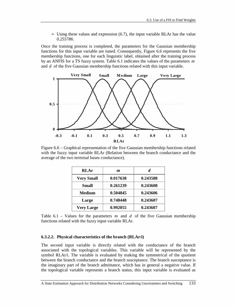
6.3. Use of a FIS to Find Weights
A State Estimation Approach for Distribution Networks Considering Uncertainties and Switching 133
−−−− Using these values and expression (6.7), the input variable RLAr has the value 0.255786.
Once the training process is completed, the parameters for the Gaussian membership functions for this input variable are tuned. Consequently, Figure 6.6 represents the five membership functions, one for each linguistic label, obtained after the training process by an ANFIS for a TS fuzzy system. Table 6.1 indicates the values of the parameters m and d of the five Gaussian membership functions related with this input variable.
0
0.5
1
-0.3 -0.1 0.1 0.3 0.5 0.7 0.9 1.1 1.3RLAr
Very Small Small M edium Large Very Large
Figure 6.6 – Graphical representation of the five Gaussian membership functions related with the fuzzy input variable RLAr (Relation between the branch conductance and the average of the two terminal buses conductance).
RLAr m d
Very Small 0.017638 0.243588
Small 0.261239 0.243608
Medium 0.504845 0.243606
Large 0.748448 0.243607
Very Large 0.992055 0.243607
Table 6.1 – Values for the parameters m and d of the five Gaussian membership functions related with the fuzzy input variable RLAr.
6.3.2.2. Physical characteristics of the branch (RLAr/i)
The second input variable is directly related with the conductance of the branch associated with the topological variables. This variable will be represented by the symbol RLAr/i. The variable is evaluated by making the symmetrical of the quotient between the branch conductance and the branch susceptance. The branch susceptance is the imaginary part of the branch admittance, which has in general a negative value. If the topological variable represents a branch status, this input variable is evaluated as

Chapter 6. Tuning the Algorithm with a Fuzzy Inference System
134 A State Estimation Approach for Distribution Networks Considering Uncertainties and Switching
indicated. Alternatively, if the topological variable represents a single switching device, the value of this input variable is zero.
The RLAr/i variable is important to get information about the type of branch. A large value means that the branch has a conductance larger than the susceptance and, of course, the branch has a resistance larger than the reactance. On the other hand, a small value for this input variable means that the branch has a susceptance larger than the conductance and, of course, the branch has a reactance larger than the resistance.
Let us consider the network of Figure 6.5. As an example, for the suspicious status of line 8, this input variable is evaluated in the following way:
−−−− The conductance value of line 8 is 1.025738 p.u.;
−−−− The susceptance value of line 8 is -4.235920 p.u.;
242152.0235920.4
025738.1 8) line(i/RLAr =
−−= (6.8)
−−−− Using these values and expression (6.8), the input variable RLAr/i has the value 0.242152.
As for the previous variable, once the training process is completed, the parameters for the Gaussian membership functions for this input variable are tuned. Consequently, Figure 6.7 represents the five membership functions, one for each linguistic label, obtained after the training process by an ANFIS for a TS fuzzy system. Table 6.2 indicates the values of the parameters m and d of the five Gaussian membership functions related with this input variable.
0
0.5
1
-1 0 1 2 3 4RLAr/i
Very Small Small M edium Large Very Large
Figure 6.7 – Graphical representation of the five Gaussian membership functions related with the fuzzy input variable RLAr/i (Relation between the branch conductance and the branch susceptance).

6.3. Use of a FIS to Find Weights
A State Estimation Approach for Distribution Networks Considering Uncertainties and Switching 135
RLAr/i m d
Very Small 0.005057 0.700349
Small 0.705427 0.700414
Medium 1.405840 0.700394
Large 2.106233 0.700393
Very Large 2.806626 0.700392
Table 6.2 – Values for the parameters m and d of the five Gaussian membership functions related with the fuzzy input variable RLAr/i.
6.3.2.3. Voltage deviation level of the area (VoltageDLevel)
The third input variable is related with the voltage level in the area nearby the topological variables, and it will be represented by VoltageDLevel. This variable is evaluated by making the average between the bus voltage magnitude on the two terminal buses of the equipment associated to the topological variable, and to this average it is then subtracted 1.0. If the topological variable represents a branch status, this variable is evaluated using the voltage magnitudes in the two extreme buses of the branch. Alternatively, if the topological variable represents a single switching device, this variable is evaluated using the voltage magnitudes in the two extreme buses of the switching device.
The voltage magnitude values used to evaluate this input variable can be a measured value, if at the bus exists a measurement device or if the voltage is specified using a pseudo-measurement. Otherwise, the value used can be a result from a previous run of the state estimation. If none of these situations is possible for the two buses, but only one bus has a voltage magnitude measurement, instead of making the average minus 1.0, the input variable is assigned the only available value minus 1.0. If no values are available for the two buses, this input variable must be considered as having zero value. In all these situations the voltage values are considered in per unit (p.u.).
The VoltageDLevel variable is important to measure the voltage level of the area where the topological variable is included. A large value means that the two terminal buses have a large voltage level eventually meaning that there is an injection point near the topological variable. On the other hand, a small value means that the two terminal buses have a lower voltage level eventually meaning there is no injection points near the topological variable.
Let us consider once again the network in Figure 6.5. As an example, for the suspicious status of line 8, this input variable is evaluated in the following way:
−−−− Line 8 is connected between buses 3 and 6, for that reason:
■ Voltage magnitude in bus 3 obtained in the previous state estimation run has the value 1.027467 p.u.;
■ Voltage magnitude in bus 6 obtained in the previous state estimation run has the value 1.004376 p.u.;

Chapter 6. Tuning the Algorithm with a Fuzzy Inference System
136 A State Estimation Approach for Distribution Networks Considering Uncertainties and Switching
015922.012
004376.1027467.1)8line(velVoltageDLe =−+= (6.9)
−−−− Using these values and expression (6.9), the input variable VoltageDLevel has the value 0.015922.
Like with previous variables, once the training process is complete, the parameters for the Gaussian membership functions for this input variable are tuned. Consequently, Figure 6.8 represents the five membership functions, one for each linguistic label, obtained after the training process by an ANFIS for a TS fuzzy system. Table 6.3 indicates the values of the parameters m and d of the five Gaussian membership functions related with this input variable.
0
0.5
1
-0.2 -0.15 -0.1 -0.05 0 0.05 0.1VoltageDLevel
Very Small Small M edium Large Very Large
Figure 6.8 – Graphical representation of the five Gaussian membership functions related with the fuzzy input variable VoltageDLevel (average of the two differences for the nominal voltage in the terminal buses).
VoltageDLevel m d
Very Small -0.141213 0.054194
Small -0.087017 0.054192
Medium -0.032816 0.054185
Large 0.021373 0.054190
Very Large 0.075563 0.054211
Table 6.3 – Values for the parameters m and d of the five Gaussian membership functions related with the fuzzy input variable VoltageDLevel.
6.3.2.4. Load level of the extreme buses (LoadLevel)
The fourth input variable is related with the load level in the two terminal buses of the equipment associated to the topological variables, and it will be represented by the

6.3. Use of a FIS to Find Weights
A State Estimation Approach for Distribution Networks Considering Uncertainties and Switching 137
symbol LoadLevel. This variable is evaluated by making the average between the active power consumption on the two terminal buses of the equipment associated to the topological variable. If the topological variable represents a branch status, this input variable is evaluated using the active power consumptions in the two extreme buses of the branch. Alternatively, if the topological variable represents a single switching device, this input variable is evaluated using the active power consumptions in the two extreme buses of the switching device.
The active power consumption value used to evaluate this variable can be a measured value, if in the bus a measurement device exists or if the active power is specified using a pseudo-measurement. Otherwise, the value used can be a result from a previous run of the state estimation. If none of these situations is possible for the two buses, but only one bus has an active power measurement, instead of making the average, the input variable is assigned the only available value. If no values are available for the two buses a load allocation procedure can be used to define values for the active power consumption in the two buses. In any case, all these values are considered in per unit (p.u.).
The LoadLevel variable is important to measure the load level of the area where the topological variable is included. A large value means that the two terminal buses have a large load level. On the other hand, a small value means that the two terminal buses have a lower load level.
We consider again the network in Figure 6.5. As an example, for the suspicious status of line 8, this input variable is evaluated in the following way:
−−−− Line 8 is connected between buses 3 and 6, for that reason:
■ Active power consumption in bus 3 from the measurement device has the value 0.120032 p.u.;
■ Active power consumption in bus 8 from the measurement device has the value 0.070028 p.u.;
095030.02
070028.0120032.0 8) line(LoadLevel =+= (6.10)
−−−− Using these values and expression (6.10), the input variable LoadLevel has the value 0.095030.
Once the training process is complete, the parameters for the Gaussian membership functions for this input variable are tuned. Consequently, Figure 6.9 represents the five membership functions, one for each linguistic label, obtained after the training process by an ANFIS for a TS fuzzy system. Table 6.4 indicates the values of the parameters m and d of the five Gaussian membership functions related with this input variable.
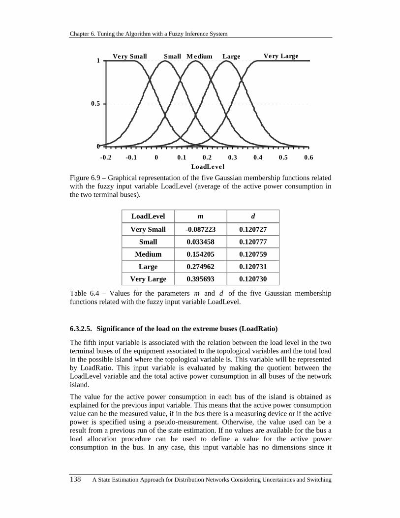
Chapter 6. Tuning the Algorithm with a Fuzzy Inference System
138 A State Estimation Approach for Distribution Networks Considering Uncertainties and Switching
0
0.5
1
-0.2 -0.1 0 0.1 0.2 0.3 0.4 0.5 0.6LoadLevel
Very Small Small M edium Large Very Large
Figure 6.9 – Graphical representation of the five Gaussian membership functions related with the fuzzy input variable LoadLevel (average of the active power consumption in the two terminal buses).
LoadLevel m d
Very Small -0.087223 0.120727
Small 0.033458 0.120777
Medium 0.154205 0.120759
Large 0.274962 0.120731
Very Large 0.395693 0.120730
Table 6.4 – Values for the parameters m and d of the five Gaussian membership functions related with the fuzzy input variable LoadLevel.
6.3.2.5. Significance of the load on the extreme buses (LoadRatio)
The fifth input variable is associated with the relation between the load level in the two terminal buses of the equipment associated to the topological variables and the total load in the possible island where the topological variable is. This variable will be represented by LoadRatio. This input variable is evaluated by making the quotient between the LoadLevel variable and the total active power consumption in all buses of the network island.
The value for the active power consumption in each bus of the island is obtained as explained for the previous input variable. This means that the active power consumption value can be the measured value, if in the bus there is a measuring device or if the active power is specified using a pseudo-measurement. Otherwise, the value used can be a result from a previous run of the state estimation. If no values are available for the bus a load allocation procedure can be used to define a value for the active power consumption in the bus. In any case, this input variable has no dimensions since it
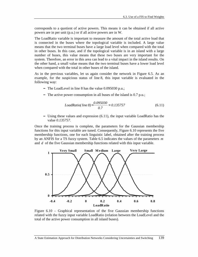
6.3. Use of a FIS to Find Weights
A State Estimation Approach for Distribution Networks Considering Uncertainties and Switching 139
corresponds to a quotient of active powers. This means it can be obtained if all active powers are in per unit (p.u.) or if all active powers are in W.
The LoadRatio variable is important to measure the amount of the total active load that is connected in the buses where the topological variable is included. A large value means that the two terminal buses have a large load level when compared with the total in other buses. In this case, and if the topological variable is in an island with a large number of buses, this value means that these two buses are very important for the system. Therefore, an error in this area can lead to a vital impact in the island results. On the other hand, a small value means that the two terminal buses have a lower load level when compared with the total in other buses of the island.
As in the previous variables, let us again consider the network in Figure 6.5. As an example, for the suspicious status of line 8, this input variable is evaluated in the following way:
−−−− The LoadLevel in line 8 has the value 0.095030 p.u.;
−−−− The active power consumption in all buses of the island is 0.7 p.u.;
135757.07.0
095030.0 8) line(LoadRatio == (6.11)
−−−− Using these values and expression (6.11), the input variable LoadRatio has the value 0.135757.
Once the training process is complete, the parameters for the Gaussian membership functions for this input variable are tuned. Consequently, Figure 6.10 represents the five membership functions, one for each linguistic label, obtained after the training process by an ANFIS for a TS fuzzy system. Table 6.5 indicates the values of the parameters m and d of the five Gaussian membership functions related with this input variable.
0
0.5
1
-0.4 -0.2 0 0.2 0.4 0.6 0.8LoadRatio
Very Small Small M edium Large Very Large
Figure 6.10 – Graphical representation of the five Gaussian membership functions related with the fuzzy input variable LoadRatio (relation between the LoadLevel and the total of the active power consumption in all island buses).

Chapter 6. Tuning the Algorithm with a Fuzzy Inference System
140 A State Estimation Approach for Distribution Networks Considering Uncertainties and Switching
LoadRatio m d
Very Small -0.181714 0.186288
Small 0.004577 0.186286
Medium 0.191019 0.186132
Large 0.377122 0.186318
Very Large 0.563440 0.186289
Table 6.5 – Values for the parameters m and d of the five Gaussian membership functions related with the fuzzy input variable LoadRatio.
6.3.3. OUTPUT VARIABLE AND TRAINING SET
The variable used as output is the weight that must be associated to the topological variable for the good convergence of the state estimation algorithm. This good convergence characteristic is related to the identification of the correct topology and to the lower number of iterations. Therefore, the weight for the topological variable will be the variable present in the consequent of the rules. If the FIS is a Mamdani fuzzy system, the output variable must be defined as a fuzzy number and then a defuzzyfication procedure must be used to return a crisp value for the weight. If the FIS corresponds to a TS fuzzy system, the output variable is obtained directly from the rules by using the expressions (6.4), (6.5) and (6.6).
In any case, the training set is generated by considering a set of values for the input variables together with a value for the best weight. The weight is represented by a continuous positive variable and any positive value is possible for this variable. However, for the generation of the training set it will be considered that only some values are possible. These values lie between 1 and 0.000001 and there will only be considered powers of 10 raised to integer numbers between minus six and zero. This means that the possible values to the weight are only seven values: 1, 0.1, 0.01, 0.001, 0.0001, 0.00001 and 0.000001.
For representation purposes, instead of considering for the output variable the value of the weight, it will be considered the decimal logarithmic of the weight. This means that the output value from the FIS is not the weight but the decimal logarithmic value of the weight. To obtain the weight one must simply compute the power of 10 raised to the result.
The generation of the training set, for each set of input variables, is performed automatically by running seven state estimation procedures, one for each weight considered. Afterwards, the weight or the weights for which the results are better are selected as the output for the input values. By changing the input values, a set to train a FIS is generated. To change the input values one must only change the values of the loads, the characteristics of the lines, the voltage level in the reference buses, and consider some different networks to consider different topologies.
The training set used to obtain the FIS has 14993 points, where each point is defined by 5 values for the input variables and a value for the output variable. Table 6.6 represents

6.3. Use of a FIS to Find Weights
A State Estimation Approach for Distribution Networks Considering Uncertainties and Switching 141
some points, more exactly 10 points, included in the training set. As an example, the values in the first row of the table mean that the branch where the topological variable is, has the variables RLAr equal to 0.394226 and RLAr/i equal to 0.240658. The voltage has values such that VoltageDLevel is equal to -0.014839. The load of the network is such that LoadLevel is equal to 0.000193 and LoadRatio is equal to 0.000743. For that
input values the best weight, among the considered weights, is 610000001.0 −= , and consequently the last value of the first row is -6.
point# RLAr RLAr/i VoltageDLevel LoadLevel LoadRatio weight
1 0.394226 0.240658 -0.014839 0.000193 0.000743 -6
2 0.399249 0.247991 -0.049875 -0.001688 -0.001624 -6
3 0.383486 0.234594 -0.046232 -0.000650 -0.000500 -6
4 0.388577 0.241800 -0.006563 -0.000299 -0.000384 -4
5 0.388577 0.241800 -0.035554 -0.004083 -0.003141 -3
6 0.122131 0.109201 -0.032132 -0.026588 -0.034087 -2
7 0.056328 0.072349 -0.007535 0.000584 0.001124 -4
8 0.054655 0.070285 -0.012423 0.000921 0.001181 -1
9 0.053823 0.069258 -0.011029 0.000426 0.000410 -6
10 0.031125 0.052933 -0.018505 0.000477 0.001835 -6
… … … … … … …
Table 6.6 – Some points used in the training set for the FIS.
Let us now consider that the inference system used is of Mamdani type, and that the output variable is described by seven membership functions with Gaussian form. After the training process, we obtained the parameters for these functions. In Figure 6.11 we present the membership functions of these seven Gaussian membership functions of the weight using a decimal logarithmic scale. This makes it easier to represent these membership functions in a graphic way. The adoption of a logarithmic scale also contributes to solve another difficulty due to the symmetrical nature of Gaussian functions. In fact, if not using this logarithmic scale, each function would be defined for the whole range of weights from 0 to 1. Since, in practice, the weights are located near zero, a large number of membership functions would be located near zero turning the results hardly possible to be interpreted. The adoption of a logarithmic scale leads to a homogenous distribution of the membership functions from –7 to 1.
On the other hand, if the inference system used is a TS fuzzy system, the output variable will be obtained directly from the consequent of the rules, calculated by a function of the input values. After the training process, the coefficients for these functions are obtained. In the next section we will describe some rules obtained for this system. By looking at these rules, it is possible to notice the influence of the different input variables in the output. This influence is transmitted by the values of the coefficients. The final weight
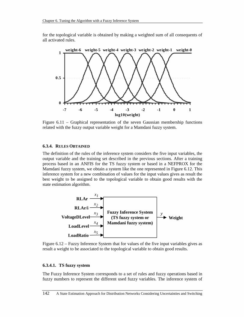
Chapter 6. Tuning the Algorithm with a Fuzzy Inference System
142 A State Estimation Approach for Distribution Networks Considering Uncertainties and Switching
for the topological variable is obtained by making a weighted sum of all consequents of all activated rules.
0
0.5
1
-7 -6 -5 -4 -3 -2 -1 0 1log10(weight)
weight-6 weight-5 weight-4 weight-3 weight-0weight-1weight-2
Figure 6.11 – Graphical representation of the seven Gaussian membership functions related with the fuzzy output variable weight for a Mamdani fuzzy system.
6.3.4. RULES OBTAINED
The definition of the rules of the inference system considers the five input variables, the output variable and the training set described in the previous sections. After a training process based in an ANFIS for the TS fuzzy system or based in a NEFPROX for the Mamdani fuzzy system, we obtain a system like the one represented in Figure 6.12. This inference system for a new combination of values for the input values gives as result the best weight to be assigned to the topological variable to obtain good results with the state estimation algorithm.
Fuzzy Inference System (TS fuzzy system or
Mamdani fuzzy system) Weight
RLAr
RLAr/i
VoltageDLevel
LoadLevel
LoadRatio
1x
2x
3x
4x
5x
y
Figure 6.12 – Fuzzy Inference System that for values of the five input variables gives as result a weight to be associated to the topological variable to obtain good results.
6.3.4.1. TS fuzzy system
The Fuzzy Inference System corresponds to a set of rules and fuzzy operations based in fuzzy numbers to represent the different used fuzzy variables. The inference system of

6.3. Use of a FIS to Find Weights
A State Estimation Approach for Distribution Networks Considering Uncertainties and Switching 143
type TS has rules like those that are represented by expression (6.3). The total number of rules obtained for this system was 256 rules. Some of these rules, more exactly 10 rules, are represented in Table 6.7. A generic rule for this system is represented by expression (6.12). In this expression: ijA can have the linguistic value VerySmall, Small, Medium,
Large or VeryLarge; 1x is the variable RLAr, 2x is the variable RLAr/i, 3x is the
variable VoltageDLevel, 4x is the variable LoadLevel and 5x id the variable LoadRatio.
5j54j43j32j21j1j0j
j55j44j33j22j11
xaxaxaxaxaay
is Ax is Ax is Ax is Ax is Ax
+++++= THEN
AND AND AND AND IF (6.12)
As an example, the first row in Table 6.7 corresponds to the rule represented by (6.13). To each of the linguistic labels that appear in the rules it is associated a membership function that was presented when the input variables were described.
Rule# 1x 2x 3x 4x 5x jy
1 Medium VerySmall Medium Small Small -2.24081 +0.093616 1x -0.086654 2x
-0.004344 3x +0.081907 4x -0.029661 5x
2 Small VerySmall Large Small Small -3.931146 +0.053003 1x +0.013158 2x
-0.085609 3x -0.044722 4x -0.034429 5x
3 VeryLarge VerySmall Medium Large Large -1.986407 -0.070798 1x +0.061146 2x
-0.07328 3x +0.044333 4x +0.058285 5x
4 Medium Medium Large Small Small -3.425492 -0.074884 1x -0.027902 2x
+0.072456 3x +0.038099 4x -0.08833 5x
5 Large VerySmall Small Large Large -1.898921 -0.086424 1x -0.044003 2x
+0.010467 3x -0.039017 4x -0.040638 5x
6 VeryLarge VerySmall Medium Medium Medium -2.651554 +0.066545 1x -0.022055 2x
-0.059652 3x +0.09139 4x +0.096496 5x
7 VeryLarge Small Small Medium Medium -0.912832 -0.016662 1x -0.04859 2x
+0.030806 3x -0.09544 4x -0.099458 5x
8 VeryLarge Large Small Large Medium -0.916422 -0.013741 1x -0.036931 2x
-0.010297 3x +0.028395 4x -0.038957 5x
9 VeryLarge Medium Medium Large Large -2.507903 -0.062563 1x +0.053205 2x
-0.081182 3x -0.035094 4x -0.011131 5x
10 VerySmall VerySmall Medium Medium Medium -1.622042 +0.02121 1x -0.081252 2x
+0.018248 3x -0.08381 4x +0.063932 5x
… … … … … … …
Table 6.7 – Some rules obtained after the training process by an ANFIS for a TS fuzzy system.
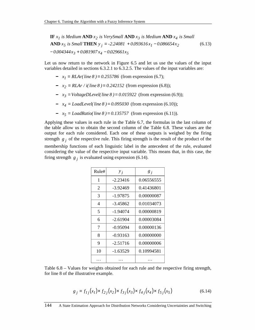
Chapter 6. Tuning the Algorithm with a Fuzzy Inference System
144 A State Estimation Approach for Distribution Networks Considering Uncertainties and Switching
543
21j5
4321
x029661.0x081907.0x004344.0
x086654.0x093616.0 24081.2-y is Smallx
is Smallx is Mediumxall is VerySmx is Medium x
−+−
−+= THEN AND
AND AND ANDIF
(6.13)
Let us now return to the network in Figure 6.5 and let us use the values of the input variables detailed in sections 6.3.2.1 to 6.3.2.5. The values of the input variables are:
−−−− 255786.0)8line(RLArx1 == (from expression (6.7);
−−−− 242152.0)8line(i/RLArx2 == (from expression (6.8));
−−−− 015922.0)8line(velVoltageDLex3 == (from expression (6.9));
−−−− 095030.0)8line(LoadLevelx4 == (from expression (6.10));
−−−− 135757.0)8line(LoadRatiox5 == (from expression (6.11)).
Applying these values in each rule in the Table 6.7, the formulas in the last column of the table allow us to obtain the second column of the Table 6.8. These values are the output for each rule considered. Each one of these outputs is weighed by the firing strength jg of the respective rule. This firing strength is the result of the product of the
membership functions of each linguistic label in the antecedent of the rule, evaluated considering the value of the respective input variable. This means that, in this case, the firing strength jg is evaluated using expression (6.14).
Rule# jy jg
1 -2.23416 0.06556555
2 -3.92469 0.41436801
3 -1.97875 0.00000087
4 -3.45862 0.01034073
5 -1.94074 0.00000819
6 -2.61904 0.00003084
7 -0.95094 0.00000136
8 -0.93163 0.00000000
9 -2.51716 0.00000006
10 -1.63529 0.10994581
… … …
Table 6.8 – Values for weights obtained for each rule and the respective firing strength, for line 8 of the illustrative example.
( ) ( ) ( ) ( ) ( )5j54j43j32j21j1j xfxfxfxfxfg ××××= (6.14)

6.3. Use of a FIS to Find Weights
A State Estimation Approach for Distribution Networks Considering Uncertainties and Switching 145
As an example, the evaluation of the firing strength for the first rule 1g is obtained by the following steps:
−−−− is Mediumx1 , therefore ( )2
1
243606.0
504845.0x
111 exf
−
−= . As the value of 1x is
equal to 0.255786 then this function ( )255786.0f11 =0.35160;
−−−− all is VerySmx2 , therefore ( )2
2
700349.0
005057.0x
221 exf
−
−= . As the value of 2x is
equal to 0.242152 then this function ( )242152.0f21 =0.89172;
−−−− is Mediumx3 , therefore ( )2
3
054185.0
032816.0x
331 exf
+−
= . As the value of 3x is
equal to 0.015922 then this function ( )015922.0f31 =0.44528;
−−−− is Smallx4 , therefore ( )2
4
120777.0
033458.0x
441 exf
−−
= . As the value of 4x is
equal to 0.095030 then this function ( )095030.0f41 =0.77113;
−−−− is Smallx5 , therefore ( )2
5
186286.0
004577.0x
551 exf
−−
= . As the value of 5x is
equal to 0.135757 then this function ( )135757.0f51 =0.60904;
−−−− Applying the expression (6.14) the value for the firing strength 1g is obtained 1g =0.35160×0.89172×0.44528×0.77113×0.60904=0.065566.
The previous calculations are performed for each one of the 256 rules. After obtaining all jy and all jg the output of the TS fuzzy system is obtained by applying the
expression (6.5). The summation in the numerator of this expression can be done for all the rules, because the rules that are not activated by the values of the input variables have values of the firing strength coefficient very small, near zero. Therefore, the importance of these rules is negligible when compared with other rules.
The output for the line 8 of the example network in Figure 6.5 has the value -1.8831, which means that the weight that must be associated to the topological variable related
with line 8 is 8831.110− =0.01308881. The other lines under suspicion of this network have the following weights as output of the TS fuzzy system:
−−−− Topological variable related with line 9 has a weight associated equal to 3541.210− =0.00442486;
−−−− Topological variable related with line 10 has a weight associated equal to 5436.310− =0.00028602;
−−−− Topological variable related with line 11 has a weight associated equal to 6794.310− =0.00020922.

Chapter 6. Tuning the Algorithm with a Fuzzy Inference System
146 A State Estimation Approach for Distribution Networks Considering Uncertainties and Switching
In the example presented along this Chapter and with the weights obtained from the FIS of type TS fuzzy system described in this section, the state estimation algorithm converges in five iterations to the correct solution. In this solution, lines 8, 9 and 10 are closed, and line 11 is opened. In this case, instead of using these weights, if a very low weight (0.000001) associated to each topological variable is used, the state estimation algorithm converges in six iterations.
6.3.4.2. Mamdani fuzzy system
The inference system of the Mamdani type has rules like those that are represented by expression (6.2). The total number of rules that were obtained for this system was 256 rules. Some of these rules, more exactly 10 rules, are represented in Table 6.9. A generic rule for this system is represented by expression (6.15). In this expression: ijA can have
the linguistic value VerySmall, Small, Medium, Large or VeryLarge; jB can have the
linguistic value weight-6, weight-5, weight-4, weight-3, weight-2, weight-1, weight-0;
1x is the variable RLAr, 2x is the variable RLAr/i, 3x is the variable VoltageDLevel,
4x is the variable LoadLevel and 5x is the variable LoadRatio.
j
j55j44j33j22j11
y is B
is Ax is Ax is Ax is Ax is Ax
THEN
AND AND AND AND IF (6.15)
4t-y is weigh THEN is Mediumx AND
is Smallx AND VeryLarge is x AND is Smallx AND all is VerySmx IF
5
4321 (6.16)
Rule# 1x 2x 3x 4x 5x jy
1 VerySmall Small VeryLarge Small Medium weight-4
2 Small Large Large Small Medium weight-4
3 Small Large VeryLarge Small Medium weight-3
4 Small VeryLarge Large Small Medium weight-3
5 Small VeryLarge VeryLarge Small Medium weight-3
6 Small Medium Large Small Medium weight-4
7 Small Medium VeryLarge Small Medium weight-5
8 Large VerySmall Small Small Small weight-3
9 Large VerySmall Medium Small Small weight-1
10 Medium VerySmall Small Small Small weight-0
… … … … … … …
Table 6.9 – Some rules obtained after the training process by an NEFPROX for a Mamdani fuzzy system.

6.3. Use of a FIS to Find Weights
A State Estimation Approach for Distribution Networks Considering Uncertainties and Switching 147
As an example, the first row of Table 6.9 corresponds to the rule represented by expression (6.16). To each one of the linguistic labels that appear in the rules it is associated a membership function that was presented when describing the input variables and the output variable.
VeryLarge
0
1
-0.1 0 0.1
VoltageDLevel
0 .22555
0
1
-0.3 0.2 0.7
LoadLevel0 .69989
S mall
0
1
-1 1 3
RLAr/iS mall
0 .40671
0
1
-0.3 0.2 0 .7 1.2
RLArVerySmall
0 .31315
weight-4
0
0.5
1
-7 -5 -3 -1 1
Weights
T H
E N
0
1
-0.4 0.1 0.6
LoadRatioMedium
0.9839
0.22555
0.255786
0.242152
0.015922
0.095030
0.135757
Figure 6.13 – Example of application of one rule and the membership function for the consequent variable obtained by application of this rule to line 8 of the network in Figure 6.5.
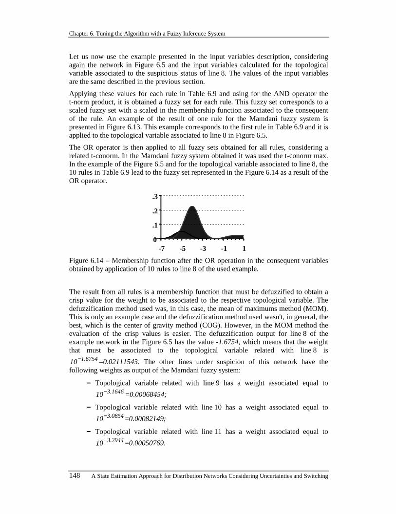
Chapter 6. Tuning the Algorithm with a Fuzzy Inference System
148 A State Estimation Approach for Distribution Networks Considering Uncertainties and Switching
Let us now use the example presented in the input variables description, considering again the network in Figure 6.5 and the input variables calculated for the topological variable associated to the suspicious status of line 8. The values of the input variables are the same described in the previous section.
Applying these values for each rule in Table 6.9 and using for the AND operator the t-norm product, it is obtained a fuzzy set for each rule. This fuzzy set corresponds to a scaled fuzzy set with a scaled in the membership function associated to the consequent of the rule. An example of the result of one rule for the Mamdani fuzzy system is presented in Figure 6.13. This example corresponds to the first rule in Table 6.9 and it is applied to the topological variable associated to line 8 in Figure 6.5.
The OR operator is then applied to all fuzzy sets obtained for all rules, considering a related t-conorm. In the Mamdani fuzzy system obtained it was used the t-conorm max. In the example of the Figure 6.5 and for the topological variable associated to line 8, the 10 rules in Table 6.9 lead to the fuzzy set represented in the Figure 6.14 as a result of the OR operator.
0
.1
.2
.3
-7 -5 -3 -1 1
Figure 6.14 – Membership function after the OR operation in the consequent variables obtained by application of 10 rules to line 8 of the used example.
The result from all rules is a membership function that must be defuzzified to obtain a crisp value for the weight to be associated to the respective topological variable. The defuzzification method used was, in this case, the mean of maximums method (MOM). This is only an example case and the defuzzification method used wasn't, in general, the best, which is the center of gravity method (COG). However, in the MOM method the evaluation of the crisp values is easier. The defuzzification output for line 8 of the example network in the Figure 6.5 has the value -1.6754, which means that the weight that must be associated to the topological variable related with line 8 is
6754.110− =0.02111543. The other lines under suspicion of this network have the following weights as output of the Mamdani fuzzy system:
−−−− Topological variable related with line 9 has a weight associated equal to 1646.310− =0.00068454;
−−−− Topological variable related with line 10 has a weight associated equal to 0854.310− =0.00082149;
−−−− Topological variable related with line 11 has a weight associated equal to 2944.310− =0.00050769.

6.4. Conclusions
A State Estimation Approach for Distribution Networks Considering Uncertainties and Switching 149
In the example presented in this Chapter and with the weights obtained from the FIS of type Mamdani fuzzy system described in this section, the state estimation algorithm converges in five iterations to the correct solution. In this solution, the lines 8, 9 and 10 are closed, and line 11 is opened.
6.4. CONCLUSIONS In this Chapter, an inference system was built that, for a set of values for five input variables, gives a weight to be associated to a topological variable. This set of values is obtained based on the characteristics of buses and branches near the device or branch with suspicious or unknown status. This inference system was created based in the experience obtained from running small examples and saving the results for each one of these examples. Thus, a large number of small examples are run with topological variables with unknown status or with suspicious status.
The inference system obtained is based on the Fuzzy Inference System theory, namely considering the ideas related to Takagi-Sugeno fuzzy systems and Mamdani fuzzy systems. In practice, it is better to use the TS fuzzy system due to the simplicity in the way that it founds a solution, and since it is more easily understood.
The great advantage of this inference system is that it is possible to find a weight for device or branch in a large network using an inference system that was never trained in that network. This means that with the knowledge obtained from small networks it is possible to infer weights for large networks only using the information in the neighbourhood of the variable under analysis. This generalisation capacity will be illustrated in the Chapter 7.
6.5. CHAPTER REFERENCES
[1] René Jager, Fuzzy Logic in Control, PhD Thesis, Technische Universiteit Delft, The Netherlands, ISBN90-9008318-9, 1995.
[2] H. Ying, "Constructing Nonlinear Variable Gain Controllers via the Takagi-Sugeno Fuzzy Control", IEEE Transactions on Fuzzy Systems, Vol. 6, No. 2, pp. 226-234, May 1998.
[3] J. Yen, L. Wang, C. W. Gillespie, "Improving the Interpretability of TSK Fuzzy Models by Combining Global Learning and Local Learning", IEEE Transactions on Fuzzy Systems, Vol. 6, No. 4, pp. 530-537, Nov. 1998.
[4] I. Rojas, H. Pomares, F. Hoffmann, F. J. Pelayo, A. Prieto, "New Design for an On-line Adaptive Fuzzy Controller", 1999 IEEE International Fuzzy Systems Conference Proceedings, Seoul, Korea, Vol. 3, pp. 1287-1292, Aug. 1999.
[5] V. Miranda, C. Monteiro, "Fuzzy Inference in Spatial Load Forecasting", Proceedings of IEEE PES Winter Meeting, Singapore, Jan. 2000.
[6] E. H. Mamdani, S. Assilian, "An experiment in linguistic synthesis with a fuzzy logic controller", International Journal of Man-Machine Studies, Vol. 7, pp. 1-13, 1975.

Chapter 6. Tuning the Algorithm with a Fuzzy Inference System
150 A State Estimation Approach for Distribution Networks Considering Uncertainties and Switching
[7] T. Takagi, M. Sugeno, "Fuzzy identification of systems and its applications to modeling and control", IEEE Transactions on Systems, Man and Cybernetics, Vol. 15, pp. 116-132, Jan. 1985.
[8] J.-S. Roger Jang, "ANFIS: Adaptive-network-based fuzzy inference systems", IEEE Transactions on Systems, Man and Cybernetics, Vol. 23, pp. 665-685, May/June 1993.
[9] D. Nauck, R. Kruse, “Neuro-Fuzzy System for Function Approximation”, Fuzzy Sets and Systems, Elsevier Science, Vol. 101, No. 2, pp. 261-271, Jan. 1999.
[10] D. Nauck, R. Kruse, “A Neuro-Fuzzy Approach to Obtain Interpretable Fuzzy Systems for Function Approximation”, Proceedings of IEEE International Conference on Fuzzy Systems 1998, pp. 1106-1111, Anchorage, May 1998.

A State Estimation Approach for Distribution Networks Considering Uncertainties and Switching 151
7. APPLICATION OF THE DEVELOPED ALGORITHMS TO AN ILLUSTRATIVE NETWORK
7.1. ILLUSTRATIVE NETWORK
7.1.1. NETWORK USED
In this Chapter, we will illustrate the application of the developed algorithms using a network based in the IEEE 24 buses network (see references [1] and [2]). The characteristics of the IEEE 24 buses network, namely branch and bus characteristics as well as power flow results, are included in the Appendix B of this Thesis.
19
17 18~
21~
22 ~
16 ~20
23 ~
1514
24 11 12
13~
3 9 10
4
12 5
7
~
8
6
138 kV230 kV
Measures: - Power - Voltage
~ Sync.Cond.
~~
~
30 kV138 kV
39
41
43
46
47
4840
51 52
49
50
42
44
45
25
27
30
34
35
2826
36 38
31
37
29
32
33
~
Figure 7.1 – Augmented network based on the IEEE 24 buses network with a new voltage level at 30 kV.

Chapter 7. Application of the Developed Algorithms to an Illustrative Network
152 A State Estimation Approach for Distribution Networks Considering Uncertainties and Switching
Using the IEEE 24 buses network and adding some buses and branches in a new voltage level of 30 kV, it is obtained the network used as an example. It was also added to this new network a branch between the buses 3 and 4. Therefore, this augment network is represented in Figure 7.1 and the purpose of this addition is to turn the original network into a more realistic case in terms of distribution networks.
The buses and branches that were considered in the voltage level of 30 kV are such that they are structured as a set of feeders operating under a radial configuration. This means that, the group composed by the buses 3, 24 and 25 represent a substation with three voltage levels (230 kV, 138 kV and 30 kV). Three feeders do the output of this substation for the 30 kV level. For that reason, this substation has two transformer groups:
−−−− One with the nominal voltages of 138 kV and 230 kV, represented in the network by the branch from bus 3 to 24;
−−−− Another with the nominal voltages of 138 kV and 30 kV, represented in the network by the branch from bus 3 to 25.
On the other hand, the group composed by the buses 6 and 39 represent a substation with two voltage levels (138 kV and 30 kV). Three feeders do the output of this substation for the 30 kV level. For that reason, this substation has one transformer group with the nominal voltages of 138 kV and 30 kV, represented in the network by the branch from bus 6 to 39.
The characteristics of this augmented network are included in the Appendix B of this Thesis. These characteristics are the generations and consumptions in all buses, the type of bus to be used for the power flow calculations and also the specified voltage when that is required, the impedance and shunt admittance of all branches, the results of the power flow for all buses and for all branches.
7.1.2. AVAILABLE MEASUREMENTS
In the representation of the example network in Figure 7.1 they are also included the available measurement devices and the respective position. The measurement devices represented are located in the buses and in the branches and they can measure the voltage magnitude or the active and reactive power.
The measurement devices installed on buses can measure the voltage magnitude and in Figure 7.1 they are represented by a black square on the buses where they are included (buses 1, 2, 3, 6, 7, 13, 15, 16 and 23). The measurement devices on buses can also measure the active and reactive power injected in the bus and in Figure 7.1 they are represented by a black circle on the bus where they are installed (buses 2, 5, 7, 8, 9, 10, 13, 15, 16 and 23). The used values for measurements obtained from these devices are given in Table 7.1.
Apart from the values obtained from the measurement devices, Table 7.1 also indicates the zero values for the power injection on some buses (buses 3, 6, 17, 24, 25 and 39). These zero values are related with the fact that these buses haven't got any power injection or power consumption. Therefore the amount of total power injected in the bus is zero.

7.1. Illustrative Network
A State Estimation Approach for Distribution Networks Considering Uncertainties and Switching 153
Bus# P
(MW) Q
(Mvar) V
(p.u.) θ Bus# P
(MW) Q
(Mvar) V
(p.u.) θ
1 - - 1.0750 0 13 276.0000 113.1027 1.0250 0 2 70.0000 91.5535 1.0750 0 15 -127.0000 98.1999 1.0250 0 3 0.0000 0.0000 0.9867 - 16 30.0000 149.1282 1.0250 0 5 -71.0000 -14.0000 - - 17 0.0000 0.0000 - - 6 0.0000 0.0000 0.9803 - 23 505.0000 48.9284 1.0250 0 7 125.0000 84.1714 1.0750 0 24 0.0000 0.0000 - - 8 -171.0000 -35.0000 - - 25 0.0000 0.0000 - - 9 -175.0000 -36.0000 - - 39 0.0000 0.0000 - -
10 -195.0000 -40.0000 - - 50 - - - 0
Table 7.1 – Values for the measurements obtained from the measurement devices in the buses. They are also indicated the zero values for the buses having zero injection and zero values for possible voltage phase references.
Bus i Bus f ifP
(MW) ifQ
(Mvar) Bus i Bus f ifP
(MW) ifQ
(Mvar)
1 3 -3.31834 46.01104 13 12 162.94350 47.43751 1 5 48.52185 57.84915 13 23 -90.8269 15.1084 2 1 -1.94377 0.09740 15 16 51.4434 -6.3363 2 4 29.63759 48.54961 15 21 -361.3526 62.4407 2 6 42.30618 42.90647 15 24 182.9092 42.0955 3 9 -4.46555 -2.89376 16 14 269.7568 60.0043 3 24 -180.66239 3.33583 16 15 -51.3871 6.7404 3 25 181.80960 41.78900 16 17 -245.8822 44.2834 6 39 137.79060 31.29180 16 19 57.5126 38.1002 7 8 125.00000 84.17138 19 20 -123.6234 0.1038 8 9 -33.33038 21.22033 20 23 -252.0033 -28.6625 8 10 -15.79444 15.90220 25 26 61.0897 12.8191 9 11 -118.40010 3.56357 25 27 54.7946 11.7541 9 12 -141.11736 3.33390 25 28 64.4919 13.8728 10 8 16.00495 -15.13301 39 40 80.8700 17.1781 12 9 141.11736 13.66939 39 41 56.9206 12.0037 13 11 203.88339 50.55681
Table 7.2 – Values for the measurements obtained from the measurement devices installed in the branches of the augmented network.
In the Table 7.1 are also represented the zero values for the voltage phase in some buses (buses 1, 2, 7, 13, 15, 16, 23, 50). In addition to these values, they are also indicated the buses that have zero values for the voltage phase pseudo-measurements. These are the buses 18, 21 and 22. These values are related with the splitting problems caused by the

Chapter 7. Application of the Developed Algorithms to an Illustrative Network
154 A State Estimation Approach for Distribution Networks Considering Uncertainties and Switching
fact of considering some uncertainty on the network topology. These buses are such that have generation capability and, in fact, these are the best buses to fix the voltage phase reference because an energised island must have at least one of these buses. The bus selected to be the phase reference for the whole network is bus 1. Of course if the network is splitted they are needed more references but these buses will be selected by the state estimation algorithm. The way that this selection is performed was described in Chapter 5 of this Thesis.
The measurement devices on the branches can measure active a reactive power flows in the branch. In this case, black circle on the branch near the bus where they are installed represents in the Figure 7.1 these measurement devices (branches 1-3, 1-5, 2-1, 2-4, 2-6, 3-9, 3-24, 3-25, 6-39, 7-8, 8-9, 8-10, 9-11, 9-12, 10-8, 12-9, 13-11, 13-12, 13-23, 15-16, 15-21, 15-24, 16-14, 16-15, 16-17, 16-19, 19-20, 20-23, 25-26, 25-27, 25-28, 39-40 and 39-41). The used values for the measurements obtained from these devices are represented in Table 7.2.
7.1.3. OBSERVABILITY ANALYSIS
With the described input information for the state estimation algorithm there are some problems related with the observability of some areas of the network. Among others, they are presented three areas that are clearly unobservable. The first area is formed by buses 18, 21 and 22, because the flow through the branches 18-21, 21-22, 17-18 and 17-22 are unobservable. The second unobservable area is formed by all feeders that leave bus 25, because they have measures only in the branches that leave this bus. Finally, the third unobservable area is formed by all feeders that leave bus 39, because they have measures only in two branches that leave this bus.
The first step to address this problem is to add more information to the set of measurements to turn the network observable. To do this we used two distinct procedures. The first procedure is to include qualitative information based in the information from the system operator or from the historical database. With this procedure, we turn observable the first identified unobservable area. The second procedure consists of running the load allocation algorithm that was described in Chapter 3 of this Thesis. As a result, we turn observable the second and the third identified unobservable areas.
7.1.3.1. Adding qualitative information
The qualitative information obtained from the system operator can correspond to information about the generation and the voltage in the buses 21 and 22. As examples, these can be characterised by the following expressions:
“The group of generators on bus 21 produces around 350 MW and this generation will not be below 315 MW nor above 385 MW. This group of generators consumes around 23 Mvar and this will not be below 20 Mvar nor above 25 Mvar”
“The connection with other network on bus 22 injects approximately 250 MW. This injection can vary by a difference from this value up to 25 MW. This connection consumes around 18 Mvar and this will not be below 16 Mvar nor above 20 Mvar”

7.1. Illustrative Network
A State Estimation Approach for Distribution Networks Considering Uncertainties and Switching 155
"The buses 21 and 22 have a voltage magnitude around 1.025 p.u., but this value can vary from 0.9225 to 1.1275 p.u."
These expressions from human language can be translated into fuzzy numbers that can be used as fuzzy measurements. A generic fuzzy number that can be used to represent each one of these fuzzy numbers is represented in Figure 7.2 and corresponds to a triangular fuzzy number. For the first expression we have two fuzzy measurements, one for the active power injected in the bus 21 and other for the reactive power injected in the same bus. In the first case, the values in Figure 7.2 will be 350 MW for the central value, 315 MW for the min and 385 MW for the max. In the case of the reactive power injection on bus 21, the values in Figure 7.2 will be -23 Mvar for the central value, -25 Mvar for the min and -20 Mvar for the max.
min central value max Figure 7.2 – Generic representation of a fuzzy measurement with a triangular membership function.
P injected (MW) Q injected (Mvar) Voltage magnitude (p.u.) Bus#
min central value
max min central value
max min central value
max
11 - - - - - - 0.9439 0.9936 1.0433 12 - - - - - - 0.9461 0.9959 1.0457 14 -213.40 -194.00 -174.60 -42.90 -39.00 -35.10 0.8946 0.9940 1.0934 18 - - - - - - 0.9738 1.0250 1.0763 21 315.00 350.00 385.00 -25.00 -23.00 -20.00 0.9225 1.0250 1.1275 22 225.00 250.00 275.00 -20.00 -18.00 -16.00 0.9225 1.0250 1.1275 24 - - - - - - 0.8962 0.9958 1.0953 50 13.50 14.20 14.90 3.40 3.60 3.80 0.9500 1.0000 1.0500
Table 7.3 – Values for the fuzzy measurements of the power injection and voltage magnitude in buses obtained from the operator information or from historical data.
The other expressions can be converted into fuzzy numbers in a similar way to the previous one. The three values needed to define a triangular fuzzy number for all the buses, where qualitative information is available like the expressions presented previously, are presented in Table 7.3. As we can see, these values can be obtained from the operator information or from the historical information in the database. In this table, examples of the fuzzy numbers obtained from the historical information in the database are, for instance, the voltage magnitude in buses 11, 12, 14 and 24.
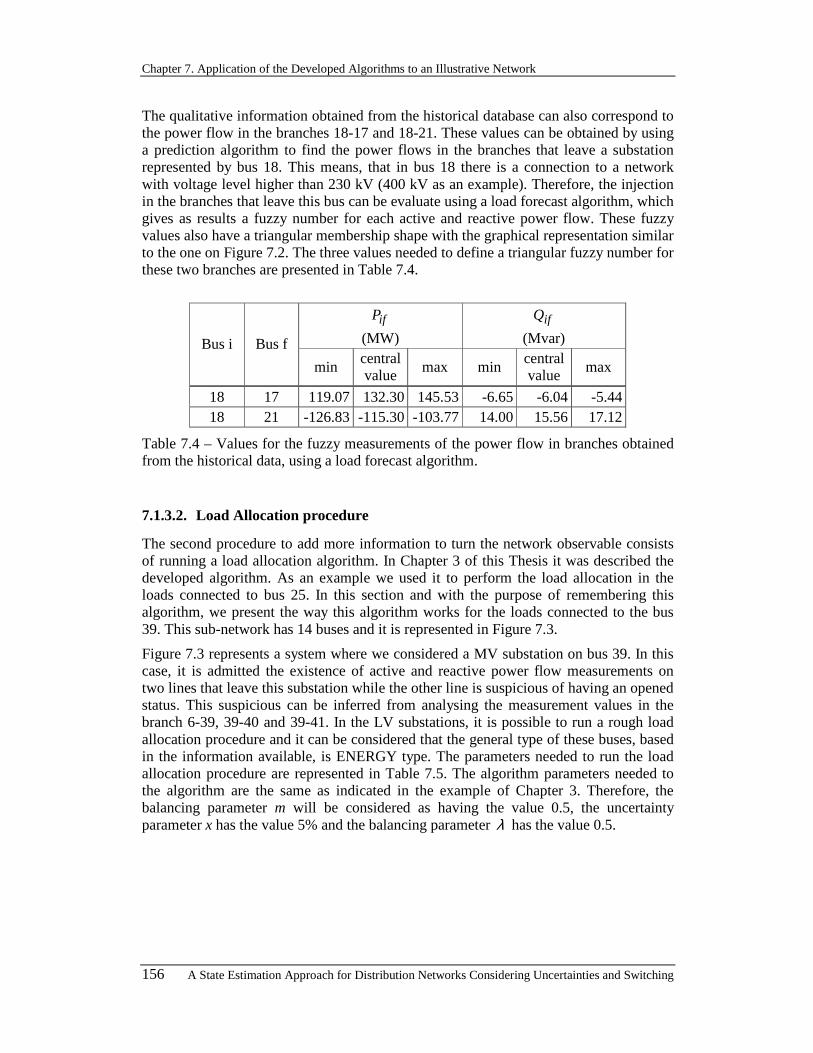
Chapter 7. Application of the Developed Algorithms to an Illustrative Network
156 A State Estimation Approach for Distribution Networks Considering Uncertainties and Switching
The qualitative information obtained from the historical database can also correspond to the power flow in the branches 18-17 and 18-21. These values can be obtained by using a prediction algorithm to find the power flows in the branches that leave a substation represented by bus 18. This means, that in bus 18 there is a connection to a network with voltage level higher than 230 kV (400 kV as an example). Therefore, the injection in the branches that leave this bus can be evaluate using a load forecast algorithm, which gives as results a fuzzy number for each active and reactive power flow. These fuzzy values also have a triangular membership shape with the graphical representation similar to the one on Figure 7.2. The three values needed to define a triangular fuzzy number for these two branches are presented in Table 7.4.
ifP
(MW) ifQ
(Mvar) Bus i Bus f
min central value
max min central value
max
18 17 119.07 132.30 145.53 -6.65 -6.04 -5.44 18 21 -126.83 -115.30 -103.77 14.00 15.56 17.12
Table 7.4 – Values for the fuzzy measurements of the power flow in branches obtained from the historical data, using a load forecast algorithm.
7.1.3.2. Load Allocation procedure
The second procedure to add more information to turn the network observable consists of running a load allocation algorithm. In Chapter 3 of this Thesis it was described the developed algorithm. As an example we used it to perform the load allocation in the loads connected to bus 25. In this section and with the purpose of remembering this algorithm, we present the way this algorithm works for the loads connected to the bus 39. This sub-network has 14 buses and it is represented in Figure 7.3.
Figure 7.3 represents a system where we considered a MV substation on bus 39. In this case, it is admitted the existence of active and reactive power flow measurements on two lines that leave this substation while the other line is suspicious of having an opened status. This suspicious can be inferred from analysing the measurement values in the branch 6-39, 39-40 and 39-41. In the LV substations, it is possible to run a rough load allocation procedure and it can be considered that the general type of these buses, based in the information available, is ENERGY type. The parameters needed to run the load allocation procedure are represented in Table 7.5. The algorithm parameters needed to the algorithm are the same as indicated in the example of Chapter 3. Therefore, the balancing parameter m will be considered as having the value 0.5, the uncertainty parameter x has the value 5% and the balancing parameter λ has the value 0.5.
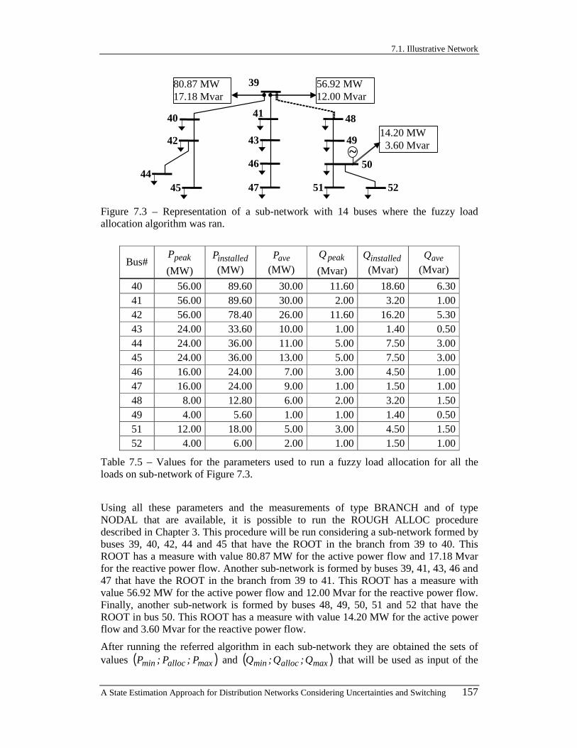
7.1. Illustrative Network
A State Estimation Approach for Distribution Networks Considering Uncertainties and Switching 157
39
41
43
46
47
4840
51 52
49
50
42
4445
~
80.87 MW17.18 Mvar
56.92 MW12.00 Mvar
14.20 MW 3.60 Mvar
Figure 7.3 – Representation of a sub-network with 14 buses where the fuzzy load allocation algorithm was ran.
Bus# peakP
(MW) installedP (MW)
aveP (MW)
peakQ
(Mvar) installedQ (Mvar)
aveQ (Mvar)
40 56.00 89.60 30.00 11.60 18.60 6.30 41 56.00 89.60 30.00 2.00 3.20 1.00 42 56.00 78.40 26.00 11.60 16.20 5.30 43 24.00 33.60 10.00 1.00 1.40 0.50 44 24.00 36.00 11.00 5.00 7.50 3.00 45 24.00 36.00 13.00 5.00 7.50 3.00 46 16.00 24.00 7.00 3.00 4.50 1.00 47 16.00 24.00 9.00 1.00 1.50 1.00 48 8.00 12.80 6.00 2.00 3.20 1.50 49 4.00 5.60 1.00 1.00 1.40 0.50 51 12.00 18.00 5.00 3.00 4.50 1.50 52 4.00 6.00 2.00 1.00 1.50 1.00
Table 7.5 – Values for the parameters used to run a fuzzy load allocation for all the loads on sub-network of Figure 7.3.
Using all these parameters and the measurements of type BRANCH and of type NODAL that are available, it is possible to run the ROUGH ALLOC procedure described in Chapter 3. This procedure will be run considering a sub-network formed by buses 39, 40, 42, 44 and 45 that have the ROOT in the branch from 39 to 40. This ROOT has a measure with value 80.87 MW for the active power flow and 17.18 Mvar for the reactive power flow. Another sub-network is formed by buses 39, 41, 43, 46 and 47 that have the ROOT in the branch from 39 to 41. This ROOT has a measure with value 56.92 MW for the active power flow and 12.00 Mvar for the reactive power flow. Finally, another sub-network is formed by buses 48, 49, 50, 51 and 52 that have the ROOT in bus 50. This ROOT has a measure with value 14.20 MW for the active power flow and 3.60 Mvar for the reactive power flow.
After running the referred algorithm in each sub-network they are obtained the sets of values ( )maxallocmin P ;P ;P and ( )maxallocmin Q ;Q ;Q that will be used as input of the

Chapter 7. Application of the Developed Algorithms to an Illustrative Network
158 A State Estimation Approach for Distribution Networks Considering Uncertainties and Switching
Fuzzy State Estimation algorithm. These values are used as fuzzy measurements having triangular membership functions. In this case, the values obtained are represented in Table 7.6.
P injected (MW) Q injected (Mvar)
Bus# min
central value
max min central value
max
40 -30.33 -29.88 -29.44 -6.25 -6.20 -6.15 41 -30.49 -29.88 -29.26 -3.55 -3.49 -3.43 42 -27.17 -26.73 -26.28 -5.75 -5.46 -5.17 43 -11.58 -10.87 -10.16 -1.71 -1.68 -1.64 44 -12.13 -11.63 -11.12 -2.93 -2.76 -2.59 45 -13.14 -12.64 -12.13 -2.93 -2.76 -2.59 46 -8.04 -7.58 -7.12 -5.12 -4.27 -3.43 47 -9.15 -8.59 -8.04 -3.43 -2.57 -1.71 48 -6.09 -5.14 -4.20 -1.20 -1.13 -1.06 49 -1.94 -1.48 -1.01 -0.49 -0.45 -0.40 51 -6.05 -5.56 -5.07 -1.53 -1.37 -1.20 52 -2.03 -2.02 -2.02 -0.80 -0.66 -0.51
Table 7.6 – Values for the pseudo-measurements obtained from the load allocation for all the loads on sub-network of Figure 7.3.
Again, it is important to notice that the Fuzzy State Estimation algorithm provides the definition of load uncertainty ranges coherent with the measurements available. Furthermore, it corrects the rough load allocation by taking into account branches losses. The correction procedure not only adjusts the estimated uncertainty at each node, but it also provides information about each branch flow and its uncertainty range.
7.1.4. TOPOLOGICAL ISSUES
The topology of the illustrative network used in this Chapter is not completely known. The status of branches 4-9, 6-10, 14-16 and 15-24 are considered to be unknown and the status of branches 3-4 and 39-48 are considered to be suspicious of having the opened status. This suspicious is inferred from analysing the measurement values, although the status for these branches in the Database is closed.
On the case of branch 3-4, bus 3 hasn't any power injection, because this bus wasn't any load or generation. This means that the power injection on the bus is zero, which means that the addition of all power flows that leave this bus must be zero. The addition of the measures on branches 1-3, 3-9, 3-24 and 3-25 for the active power flow gives a value near zero. Then branch 3-4 has a very low active power flow or it is opened. By this analysis, this branch is included in the state estimation as opened but this status can be erroneous. Consequently, the status of this branch will be included in the state vector considering a topological variable as described in Chapter 4 of this Thesis.
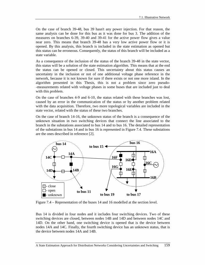
7.1. Illustrative Network
A State Estimation Approach for Distribution Networks Considering Uncertainties and Switching 159
On the case of branch 39-48, bus 39 hasn't any power injection. For that reason, the same analysis can be done for this bus as it was done for bus 3. The addition of the measures on branches 6-39, 39-40 and 39-41 for the active power flow gives a value near zero. This means that branch 39-48 has a very low active power flow or it is opened. By this analysis, this branch is included in the state estimation as opened but this status can be erroneous. Consequently, the status of this branch will be included as a state variable.
As a consequence of the inclusion of the status of the branch 39-48 in the state vector, this status will be a solution of the state estimation algorithm. This means that at the end the status can be opened or closed. This uncertainty about this status causes an uncertainty in the inclusion or not of one additional voltage phase reference in the network, because it is not known for sure if there exists or not one more island. In the algorithm presented in this Thesis, this is not a problem since zero pseudo--measurements related with voltage phases in some buses that are included just to deal with this problem.
On the case of branches 4-9 and 6-10, the status related with these branches was lost, caused by an error in the communication of the status or by another problem related with the data acquisition. Therefore, two more topological variables are included in the state vector, related with the status of these two branches.
On the case of branch 14-16, the unknown status of the branch is a consequence of the unknown situation in two switching devices that connect the line associated to the branch in the substations associated to bus 14 and to bus 16. The detailed representation of the substations in bus 14 and in bus 16 is represented in Figure 7.4. These substations are the ones described in reference [2].
14C
bus 14
to bus 11
14D
14A
14B
to bus 17to bus 19
bus 16
16Ato bus 15
16B
16C16D
16G
16F
16E
- close- open- unknown
Figure 7.4 – Representation of the buses 14 and 16 modelled at the section level.
Bus 14 is divided in four nodes and it includes four switching devices. Two of these switching devices are closed, between nodes 14B and 14D and between nodes 14C and 14D. On the other hand, one switching device is opened that is the device between nodes 14A and 14C. Finally, the fourth switching device has an unknown status, that is the device between nodes 14A and 14B.

Chapter 7. Application of the Developed Algorithms to an Illustrative Network
160 A State Estimation Approach for Distribution Networks Considering Uncertainties and Switching
Bus 16 is divided in seven nodes and it includes 8 switching devices. Five of these switching devices have a closed status. On the other hand, two switching devices have an opened status. Finally, one switching device has an unknown status, that is the device between nodes 16A and 16F.
In the configuration in Figure 7.4 these two switching devices with unknown status are precisely the switching devices that connect the line 14A-16F to the other nodes in the two substations. Therefore, instead of modelling the two switching devices with two topological variables, we modelled the status of the branch with one topological variable. The same can be done if the switching device 16F-16G has an unknown status or if the switching device 14A-14C has an unknown status, or if these two have the unknown status, or even if these two more the other two previously indicated have the unknown status.
On the case of branch 15-24, the unknown status of the branch is a consequence of the unknown situation in two switching devices that connect the line associated to the branch in the substations associated to bus 15 and to bus 24. The detailed substations in bus 15 and in bus 24 are represented in Figure 7.5. These substations are the ones described in reference [2].
bus 24
to bus 3
24A
24B
to bus 21to bus 16
bus 15
15A
15B
15C15F
15G
15H
15E 15D
- close- open- unknown
Figure 7.5 – Representation of the buses 15 and 24 modelled at the section level.
Bus 15 is divided in 8 nodes and it includes 9 switching devices. Five of these switching devices are closed. On the other hand, three switching devices are opened. Finally, the switching device between nodes 15A and 15H has an unknown status.
Bus 24 is divided in 2 nodes and it includes 2 switching devices. One of these switching devices is closed and the other, between nodes 24A and 24B, has an unknown status.
As for the branch 14-16, the same analysis can be done for branch 15-24. This means that, in the configuration in Figure 7.5, the two switching devices with unknown status are precisely the switching devices that connect the line 15H-24A to the other nodes in the two substations. Therefore, instead of modelling the two switching devices with two topological variables, we modelled the status of the branch with a single topological variable. The same can be done if the switching device 15G-15H has an unknown status or if the other switching device 24A-24B has an unknown status, or if these two have
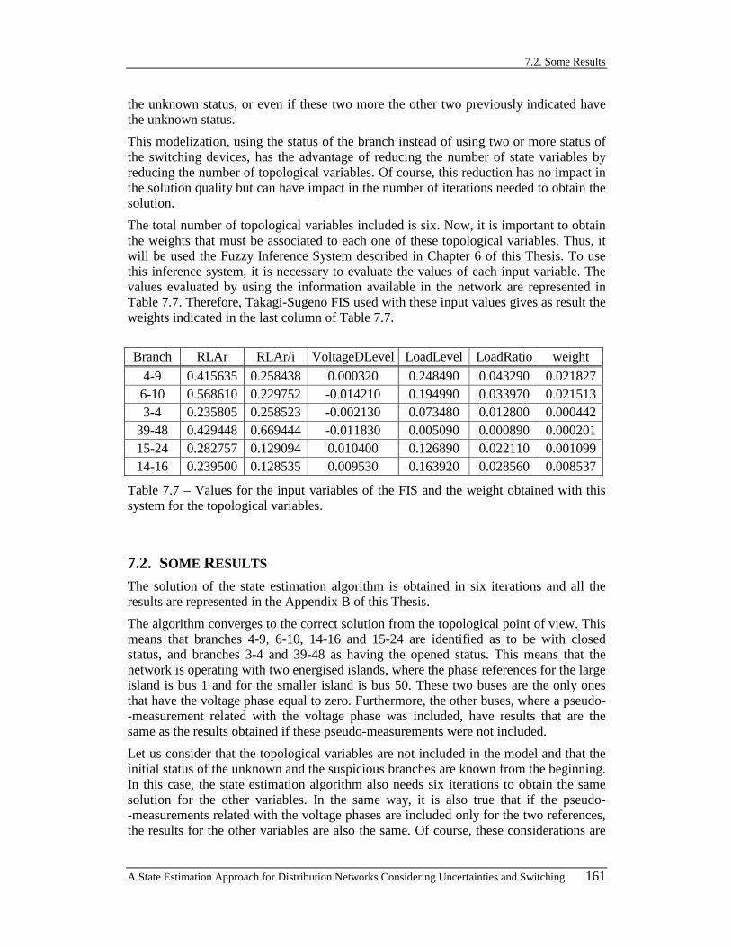
7.2. Some Results
A State Estimation Approach for Distribution Networks Considering Uncertainties and Switching 161
the unknown status, or even if these two more the other two previously indicated have the unknown status.
This modelization, using the status of the branch instead of using two or more status of the switching devices, has the advantage of reducing the number of state variables by reducing the number of topological variables. Of course, this reduction has no impact in the solution quality but can have impact in the number of iterations needed to obtain the solution.
The total number of topological variables included is six. Now, it is important to obtain the weights that must be associated to each one of these topological variables. Thus, it will be used the Fuzzy Inference System described in Chapter 6 of this Thesis. To use this inference system, it is necessary to evaluate the values of each input variable. The values evaluated by using the information available in the network are represented in Table 7.7. Therefore, Takagi-Sugeno FIS used with these input values gives as result the weights indicated in the last column of Table 7.7.
Branch RLAr RLAr/i VoltageDLevel LoadLevel LoadRatio weight
4-9 0.415635 0.258438 0.000320 0.248490 0.043290 0.021827 6-10 0.568610 0.229752 -0.014210 0.194990 0.033970 0.021513 3-4 0.235805 0.258523 -0.002130 0.073480 0.012800 0.000442
39-48 0.429448 0.669444 -0.011830 0.005090 0.000890 0.000201 15-24 0.282757 0.129094 0.010400 0.126890 0.022110 0.001099 14-16 0.239500 0.128535 0.009530 0.163920 0.028560 0.008537
Table 7.7 – Values for the input variables of the FIS and the weight obtained with this system for the topological variables.
7.2. SOME RESULTS The solution of the state estimation algorithm is obtained in six iterations and all the results are represented in the Appendix B of this Thesis.
The algorithm converges to the correct solution from the topological point of view. This means that branches 4-9, 6-10, 14-16 and 15-24 are identified as to be with closed status, and branches 3-4 and 39-48 as having the opened status. This means that the network is operating with two energised islands, where the phase references for the large island is bus 1 and for the smaller island is bus 50. These two buses are the only ones that have the voltage phase equal to zero. Furthermore, the other buses, where a pseudo--measurement related with the voltage phase was included, have results that are the same as the results obtained if these pseudo-measurements were not included.
Let us consider that the topological variables are not included in the model and that the initial status of the unknown and the suspicious branches are known from the beginning. In this case, the state estimation algorithm also needs six iterations to obtain the same solution for the other variables. In the same way, it is also true that if the pseudo--measurements related with the voltage phases are included only for the two references, the results for the other variables are also the same. Of course, these considerations are

Chapter 7. Application of the Developed Algorithms to an Illustrative Network
162 A State Estimation Approach for Distribution Networks Considering Uncertainties and Switching
only possible in an experimental case, because, as explained in this Thesis, the inclusion of these pseudo-measurements is required to deal with some problems when a real network is analysed.
Other results obtained in the state estimation algorithm are the values for the state variables related with the voltage in each bus, the power injections for each bus, power flows and current on each branch. It should be emphasised that the methodology described in Chapter 3 of this Thesis can incorporate both deterministic traditional measurements, although affected by metering errors, as well as fuzzy measurements as the ones referred before. In this case, measurement devices obtain some input data while other input data related to fuzzy measurements are obtained by the different referred sources.
In any case, as a result of the specified uncertainties, the state estimation results are also affected by uncertainty. This means that we obtain a description of the possible state of the system as a result of the referred uncertainties. The fuzzy state estimation procedure can be interpreted as a way to reflect uncertainties present on data on the usual state estimation results.
In order to illustrate this procedure, we present the membership functions of several output variables obtained from the fuzzy state estimation algorithm for the illustrative network. In some cases, when the output variable is measured, it is presented the input and the output membership functions. These membership functions have a triangular shape because the fuzzy measurements considered are all triangular fuzzy numbers. If some input variables were trapezoidal or had another shapes, the output variables would also be trapezoidal or would also have another shapes, even non-normalised ones.
0.94 0.99 1.04
V11(p.u.)
measure result
0.88 0.98 1.08
V14(p.u.)
measure
result
Figure 7.6 – Membership functions for the measurements and for the results of the voltage magnitude in the buses 11 and 14.
In Figure 7.6 they are presented the membership functions for the measures and the results obtained for the voltage magnitude in buses 11 and 14. These two voltages magnitudes are included in the input data as fuzzy measurements. The analysis of these membership functions deserves some comments. One of the most interesting features of the developed fuzzy state estimation model is that the specified fuzziness is in some cases, as the ones represented in Figure 7.6, larger than the uncertainty resulting for the same variables for the membership functions obtained at the end of the state estimation study.
This can be explained if we remember that state estimation models are a way to eliminate incoherencies in data relative to a process, in this case a power system running in a steady state. Therefore, one can think that the uncertainty ranges defined as data integrate values that are incoherent with the pattern defined by the global set of
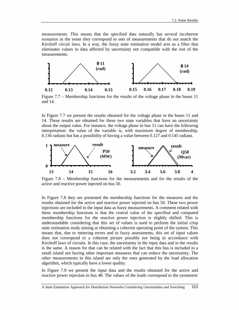
7.2. Some Results
A State Estimation Approach for Distribution Networks Considering Uncertainties and Switching 163
measurements. This means that the specified data naturally has several incoherent scenarios in the sense they correspond to sets of measurements that do not match the Kirchoff circuit laws. In a way, the fuzzy state estimation model acts as a filter that eliminates values in data affected by uncertainty not compatible with the rest of the measurements.
0.12 0.13 0.14 0.15
θ θ θ θ 11(rad)
0.15 0.16 0.17 0.18 0.19
θ θ θ θ 14(rad)
Figure 7.7 – Membership functions for the results of the voltage phase in the buses 11 and 14.
In Figure 7.7 we present the results obtained for the voltage phase in the buses 11 and 14. These results are obtained for these two state variables that have an uncertainty about the output value. For instance, the voltage phase in bus 11 can have the following interpretation: the value of the variable is, with maximum degree of membership, 0.136 radians but has a possibility of having a value between 0.127 and 0.145 radians.
0
1
13 14 15 16
resultmeasure
P50(MW)
3.2 3.4 3.6 3.8 4
resultmeasureQ50
(Mvar)
Figure 7.8 – Membership functions for the measurements and for the results of the active and reactive power injected on bus 50.
In Figure 7.8 they are presented the membership functions for the measures and the results obtained for the active and reactive power injected on bus 50. These two power injections are included in the input data as fuzzy measurements. A comment related with these membership functions is that the central value of the specified and computed membership functions for the reactive power injection is slightly shifted. This is understandable considering that this set of values is used to perform the initial crisp state estimation study aiming at obtaining a coherent operating point of the system. This means that, due to metering errors and to fuzzy assessments, this set of input values does not correspond to a coherent picture possibly not being in accordance with Kirchoff laws of circuits. In this case, the uncertainty in the input data and in the results is the same. A reason for that can be related with the fact that this bus is included in a small island not having other important measures that can reduce the uncertainty. The other measurements in this island are only the ones generated by the load allocation algorithm, which typically have a lower quality.
In Figure 7.9 we present the input data and the results obtained for the active and reactive power injection in bus 48. The values of the loads correspond to the symmetric
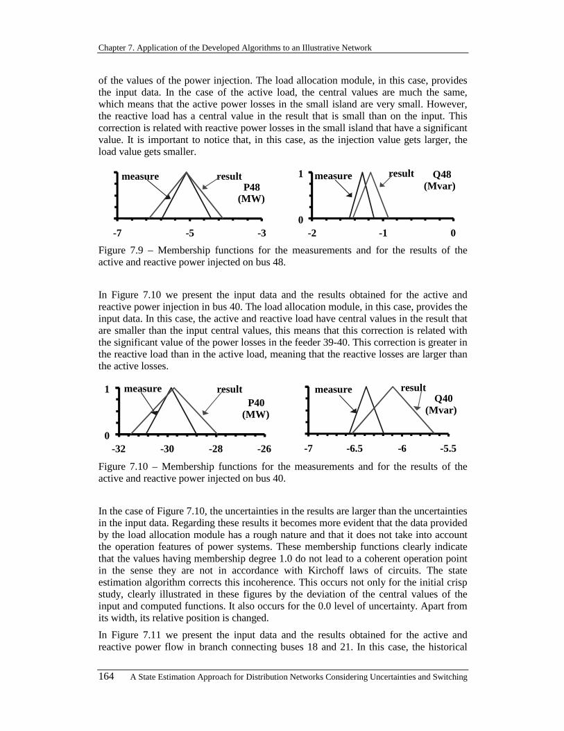
Chapter 7. Application of the Developed Algorithms to an Illustrative Network
164 A State Estimation Approach for Distribution Networks Considering Uncertainties and Switching
of the values of the power injection. The load allocation module, in this case, provides the input data. In the case of the active load, the central values are much the same, which means that the active power losses in the small island are very small. However, the reactive load has a central value in the result that is small than on the input. This correction is related with reactive power losses in the small island that have a significant value. It is important to notice that, in this case, as the injection value gets larger, the load value gets smaller.
-7 -5 -3
resultmeasureP48
(MW)
0
1
-2 -1 0
resultmeasure Q48(Mvar)
Figure 7.9 – Membership functions for the measurements and for the results of the active and reactive power injected on bus 48.
In Figure 7.10 we present the input data and the results obtained for the active and reactive power injection in bus 40. The load allocation module, in this case, provides the input data. In this case, the active and reactive load have central values in the result that are smaller than the input central values, this means that this correction is related with the significant value of the power losses in the feeder 39-40. This correction is greater in the reactive load than in the active load, meaning that the reactive losses are larger than the active losses.
0
1
-32 -30 -28 -26
resultmeasureP40
(MW)
-7 -6.5 -6 -5.5
resultmeasureQ40
(Mvar)
Figure 7.10 – Membership functions for the measurements and for the results of the active and reactive power injected on bus 40.
In the case of Figure 7.10, the uncertainties in the results are larger than the uncertainties in the input data. Regarding these results it becomes more evident that the data provided by the load allocation module has a rough nature and that it does not take into account the operation features of power systems. These membership functions clearly indicate that the values having membership degree 1.0 do not lead to a coherent operation point in the sense they are not in accordance with Kirchoff laws of circuits. The state estimation algorithm corrects this incoherence. This occurs not only for the initial crisp study, clearly illustrated in these figures by the deviation of the central values of the input and computed functions. It also occurs for the 0.0 level of uncertainty. Apart from its width, its relative position is changed.
In Figure 7.11 we present the input data and the results obtained for the active and reactive power flow in branch connecting buses 18 and 21. In this case, the historical

7.2. Some Results
A State Estimation Approach for Distribution Networks Considering Uncertainties and Switching 165
database provides the input data by defining a fuzzy measurement. The central values for the active and reactive power flow are much the same, which means that the central values are coherent with the other measurements. However, the uncertainties in the results are larger than the uncertainties in the input data. Regarding these results it becomes also evident that data, provided from the historical database, does not take into account correctly the operation features of the network.
-150 -130 -110 -90
resultmeasure P18-21
(MW)
0
1
8 13 18 23
resultmeasure Q18-21
(Mvar)
Figure 7.11 – Membership functions for the measurements and for the results of the active and reactive power flow on the branch connecting buses 18 and 21.
In Figure 7.12 we present the results obtained for the active and reactive power flow on the branch connecting buses 29 and 32. These power flows are representing by triangular membership functions reflecting the uncertainties in data. These variables are located on an extreme branch of one of the feeders that leaves the bus 25. For instance, the result for the active power flow in this branch can have the following interpretation: the value of the active power flow is 9.75 MW with 1.0 membership degree, but has a possibility of having a value between 8.29 MW and 11.21 MW.
0
1
8 10 12
P29-32(MW)
1.8 2.3 2.8
Q29-32(Mvar)
Figure 7.12 – Membership functions for the measurements and for the results of the active and reactive power flow on the branch connecting buses 29 and 32.
8 10 12
P32(MW)
0
1
1.8 2.3 2.8
Q32(Mvar)
Figure 7.13 – Membership functions for the results of the active and reactive power load on bus 32.
The branch 29-32 supplies one only load connected to bus 32. This means that the power flow through this branch is used only to supply this load. Therefore, in Figure 7.13 we present the results obtained for the active and reactive power load on bus 32.
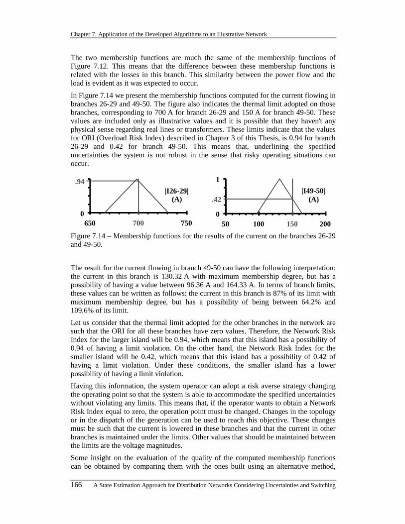
Chapter 7. Application of the Developed Algorithms to an Illustrative Network
166 A State Estimation Approach for Distribution Networks Considering Uncertainties and Switching
The two membership functions are much the same of the membership functions of Figure 7.12. This means that the difference between these membership functions is related with the losses in this branch. This similarity between the power flow and the load is evident as it was expected to occur.
In Figure 7.14 we present the membership functions computed for the current flowing in branches 26-29 and 49-50. The figure also indicates the thermal limit adopted on those branches, corresponding to 700 A for branch 26-29 and 150 A for branch 49-50. These values are included only as illustrative values and it is possible that they haven't any physical sense regarding real lines or transformers. These limits indicate that the values for ORI (Overload Risk Index) described in Chapter 3 of this Thesis, is 0.94 for branch 26-29 and 0.42 for branch 49-50. This means that, underlining the specified uncertainties the system is not robust in the sense that risky operating situations can occur.
0650 700 750
|I26-29|(A)
.94
0
1
50 100 150 200
|I49-50|(A).42
Figure 7.14 – Membership functions for the results of the current on the branches 26-29 and 49-50.
The result for the current flowing in branch 49-50 can have the following interpretation: the current in this branch is 130.32 A with maximum membership degree, but has a possibility of having a value between 96.36 A and 164.33 A. In terms of branch limits, these values can be written as follows: the current in this branch is 87% of its limit with maximum membership degree, but has a possibility of being between 64.2% and 109.6% of its limit.
Let us consider that the thermal limit adopted for the other branches in the network are such that the ORI for all these branches have zero values. Therefore, the Network Risk Index for the larger island will be 0.94, which means that this island has a possibility of 0.94 of having a limit violation. On the other hand, the Network Risk Index for the smaller island will be 0.42, which means that this island has a possibility of 0.42 of having a limit violation. Under these conditions, the smaller island has a lower possibility of having a limit violation.
Having this information, the system operator can adopt a risk averse strategy changing the operating point so that the system is able to accommodate the specified uncertainties without violating any limits. This means that, if the operator wants to obtain a Network Risk Index equal to zero, the operation point must be changed. Changes in the topology or in the dispatch of the generation can be used to reach this objective. These changes must be such that the current is lowered in these branches and that the current in other branches is maintained under the limits. Other values that should be maintained between the limits are the voltage magnitudes.
Some insight on the evaluation of the quality of the computed membership functions can be obtained by comparing them with the ones built using an alternative method,

7.3. Chapter References
A State Estimation Approach for Distribution Networks Considering Uncertainties and Switching 167
based on a gradient optimization method as described in reference [3]. The results directly obtained by the two methods are remarkably close. That is, we may be confident that the FSE results have good quality and display a good accuracy. Of course, the gradient model was developed only for the purpose of assessing this feature, since it is irrealistic to use in any real world application due to its extremely large computation burden.
7.3. CHAPTER REFERENCES
[1] IEEE RTS Task Force of APM Subcommittee, “IEEE Reliability Test System”, IEEE Transactions on Power Apparatus and Systems, Vol. 98, No. 6, pp. 2047-2054, Nov/Dec. 1979.
[2] R. Billinton, P.K. Vohra, S. Kumar, “Effect of Station Originated Outages in a Composite System Adequacy Evaluation of the IEEE Reliability Test System”, IEEE Transactions on Power Apparatus and Systems, Vol. 104, No. 10, pp. 2649-2656, Oct. 1985.
[3] Jorge Pereira, Estimação de Estado em Redes de Distribuição de Energia com Medidas Imprecisas, MSc. Thesis, Faculdade de Engenharia da Universidade do Porto, Porto, May 1995.


A State Estimation Approach for Distribution Networks Considering Uncertainties and Switching 169
8. CONCLUSIONS
8.1. GENERAL CONCLUSIONS In this Thesis we described an integrated State Estimation methodology aiming at identifying the state of distribution networks also including the identification of the topology in operation. The model is highly flexible in terms of the data it can incorporate. This can correspond to traditional real time measurements, fuzzy assessments and results from load allocation procedures. Additionally, the model has the ability to address topology issues given that in the input data, the topology of the network can be unknown in some areas. These are related with the uncertainty that may affect the knowledge about the status of switching devices and thus it is important to give the system the ability to split in several islands or to merge different input areas into larger ones, if that is more adequate to explain the available measurements. This means that we enlarged the traditional nature of WLS state estimation algorithms explicitly to deal with data having several forms of uncertainty including topology aspects. This also implies that the state of the system is not only characterised by voltages and phases but also by topology variables that are computed by the algorithm.
It should be stressed that in this approach we combine traditional WLS probabilistic algorithms with fuzzy concepts. This reflects our desire to use the most adequate mathematical tools for each particular situation, our purpose to use emergent techniques and our belief that fuzzy concepts, despite very appealing, will not replace probabilistic concepts.
The possibility of integrating fuzzy representations appears important in the scope of the move to restructure power systems. This clearly leads to a more uncertain world so that this kind of algorithms can play an important role in control centres of transmission or distribution systems. In any case, fuzzy representations are always useful if we remember that distribution networks have a small number of available measurements and that available qualitative information can be modelled by fuzzy numbers. This qualitative information can correspond to information about dispersed generation connected to the network, like wind power generation, mini-hydro power plants generation, co-generation. Other qualitative information can be related with the results of prediction modules to forecast load consumption at the substation level, which can be affected by uncertainty. The forecasted values obtained by these applications are introduced afterwards in a Fuzzy Load Allocation procedure that, as results, gives uncertain values for loads.
The referred Fuzzy Load Allocation procedure is also presented in this Thesis and it is described how from uncertain data one may produce, in a DMS environment, a consistent load allocation to system buses, so that other calculation modules may work, namely load flow routines. DMS software demands a specific Load Allocation procedure because, contrary to EMS environments for Generation / Transmission systems, there is usually a small number of real time information or load measurements in distribution systems. In this work, this algorithm was considered as a possible source of fuzzy measures for the Fuzzy State Estimation. It can also be interpreted as an

Chapter 8. Conclusions
170 A State Estimation Approach for Distribution Networks Considering Uncertainties and Switching
algorithm that allocates values to loads in order to subsequently activate the Fuzzy State Estimation as a corrective procedure for the rough loads initially allocated.
In this scope, the solution conceived for the Fuzzy Load Allocation algorithm, making use of Fuzzy State Estimation concepts, guarantees not only a load allocation where total load matches power injections, but also where flows are described by the possible ranges compatible with actual measurements in the distribution network. These can correspond to traditional radial systems or to meshed networks, without posing any problem to the formulation.
The results of the State Estimation algorithm give not only an indication of some range of uncertainty on estimated variables, but also allows operators to become aware of levels of risk and possible alarms, if the combination of uncertainties open the possibility to have branch limits to be surpassed by power flows or to have violation of nodal voltage ranges.
Regarding topology issues, it should be pointed out the novel, mathematically sounded and computationally efficient treatment given to uncertainties affecting the current status of switching devices and the new and effective way adopted to address numerical problems due to system splitting. To solve the unknown topology problem, they are included in the formulation some topological variables as state variables. These variables have continuous nature but they are constrained so that in the results they assume the value 0 - open or 1 - close. With this approach we obtain good results to identify the topology along with the estimation of the other state variables. This means that the identified solution will correspond to the topology that better adjusts to the available information. The topology is not a priori fixed, but it will result from the state estimation run.
The consideration of uncertainty on the topology in operation introduces the system splitting difficulty related with the fact that, at the beginning, it may not be possible to know how many islands there are actually in the network. Consequently, it is not possible to know how many voltage phase references are required. The solution presented for this problem corresponds to consider several voltage phase pseudo--measurements with zero values. This approach allow us to obtain very good results because the number of references is always the same as the number of energised islands, and the pseudo-measurements that are not used have no influence in the final results.
This Thesis also describes an inference system that was built to generate the weight to assign to each topological variable, based on a set of values for five input variables. This set of values is obtained based on the characteristics of buses and branches near the device or branch with suspicious or unknown status. This inference system was created based in the experience obtained from running a large number of small examples and saving the results for each one of them. Thus, a large number of small examples are run with topological variables with unknown status or with suspicious status. The inference system obtained is based on the Fuzzy Inference System Theory, namely considering the ideas related to Takagi-Sugeno (TS) fuzzy systems. It is used a TS fuzzy system due to the simplicity in the way that it founds a solution, and since it is more easily understood.
The great advantage of this inference system is that it is possible to assign a weight for a device or branch in a large network using an inference system that was never trained for that network, but rather for small networks. This means that with the knowledge obtained from small networks it is possible to infer weights for large networks only

8.2. Perspectives of Future Work
A State Estimation Approach for Distribution Networks Considering Uncertainties and Switching 171
using the information in the neighbourhood of the variable under analysis. This system was used in the illustrative network referred in Chapter 7 of this Thesis and the identified solution was the correct one from the topological point of view. The application of this inference system to other networks allow us to conclude that it works well and that it can be applied in any network regardless of its size.
Some interesting results are presented in Chapter 7 and Appendix B for the illustrative network. Among them, we can refer the fact that the Fuzzy State Estimation model allows in some cases to narrow the range of uncertainty present in the input fuzzy data. This may represent a new way of improving the consistency of historical file for loads that are not directly monitored, which could be of great interest in managing distribution systems.
This kind of State Estimation applications has a large potential of use in the future given that they are more adapted to represent reality in a closer way and that they provide a more complete knowledge about the system in operation. It should be referred that the algorithm is computationally very efficient since, in average, the surplus of execution time when compared with traditional WLS approaches is very low. From several experimental runs, we got an average figure of only more 55% computational time when comparing the developed Fuzzy approach with traditional WLS models. This seems a well reduced price to pay when considering the more complete knowledge about system behaviour that is provided and the possibility of running the module even if the topology is not completely unknown.
It must be said that the Fuzzy State Estimation model is not specific of distribution systems, and it can be applied directly to transmission systems and included in EMS environments, adding either its switch status variable handling ability or its fuzzy data representation capacity.
Finally, it is important to say that some ideas of the model described in this Thesis have already been integrated in a DMS package offered in the market, applied in some utilities in the world, making it not only a theoretical exercise, but a case of successful transfer of knowledge to industry.
8.2. PERSPECTIVES OF FUTURE WORK The subject of this Thesis was extensive and ambitious. Therefore it will not be a surprise to enumerate some aspects that were not covered as deeply as one could expect. Apart from that, some ideas developed in this research can be applied in other areas.
Among other aspects that could be further developed, the author would like to refer the following possible developments:
−−−− Modern control centres for distribution systems are integrating a more and more detailed network representation and, in some cases, they integrate parts of the generation / production system as well as LV networks. This leads to the large increase of the network size turning it eventually difficult to run the State Estimation algorithm in the entire network. Therefore, the network should be separated so that the State Estimation runs rapidly in each sub-network. This division must be done in such a way that the global solution must be always the same as if the entire network as treated by a single run. This separation algorithm must deal with unknown topology problem;

Chapter 8. Conclusions
172 A State Estimation Approach for Distribution Networks Considering Uncertainties and Switching
−−−− The developed approach was done based in the State Estimation algorithm using the Weighted Least Squares Method. The application of the developed methodology to other State Estimation approaches problem is possible after some modifications. The alternative approaches can be the based on the Weighted Least Absolute Values Method or on the Orthogonal Factorization Method. The ideas to be applied in these methods would include fuzzy measurements, topological variables and pseudo-measurements to deal with splitting problems;
−−−− Using the ideas that lead to the fuzzy inference system developed to assign weights to the topological variables, an important line of research would correspond to analyse the application of the same concepts to other kind of algorithms. This means that, when it is required a procedure to control an algorithm convergence by changing some variables, a fuzzy inference system trained for small examples can eventually be used for this purpose. This application can be explored not only in the scope of power systems problems, but eventually in other areas;
−−−− The same can be said for topological variables. The ideas included in this Thesis to address the problem related with binary behaviours correspond to the adoption of constrained continuous variables. This preserves the continuous nature of formulations turning it unnecessary the use of time consuming methods to solve integer or binary problems.
At the end of these six years of research, a long way was covered, from simple and traditional applications to more involving and closer to reality ones. Despite the rapid changes in our world, the developed models can be of use, and in some cases are already being used, in real control centres. This is a new route to follow in next years going on reducing the gap between theoretical models and real applications. I hope this Thesis is a contribution to this global objective.

A State Estimation Approach for Distribution Networks Considering Uncertainties and Switching 173

174 A State Estimation Approach for Distribution Networks Considering Uncertainties and Switching
APPENDICES
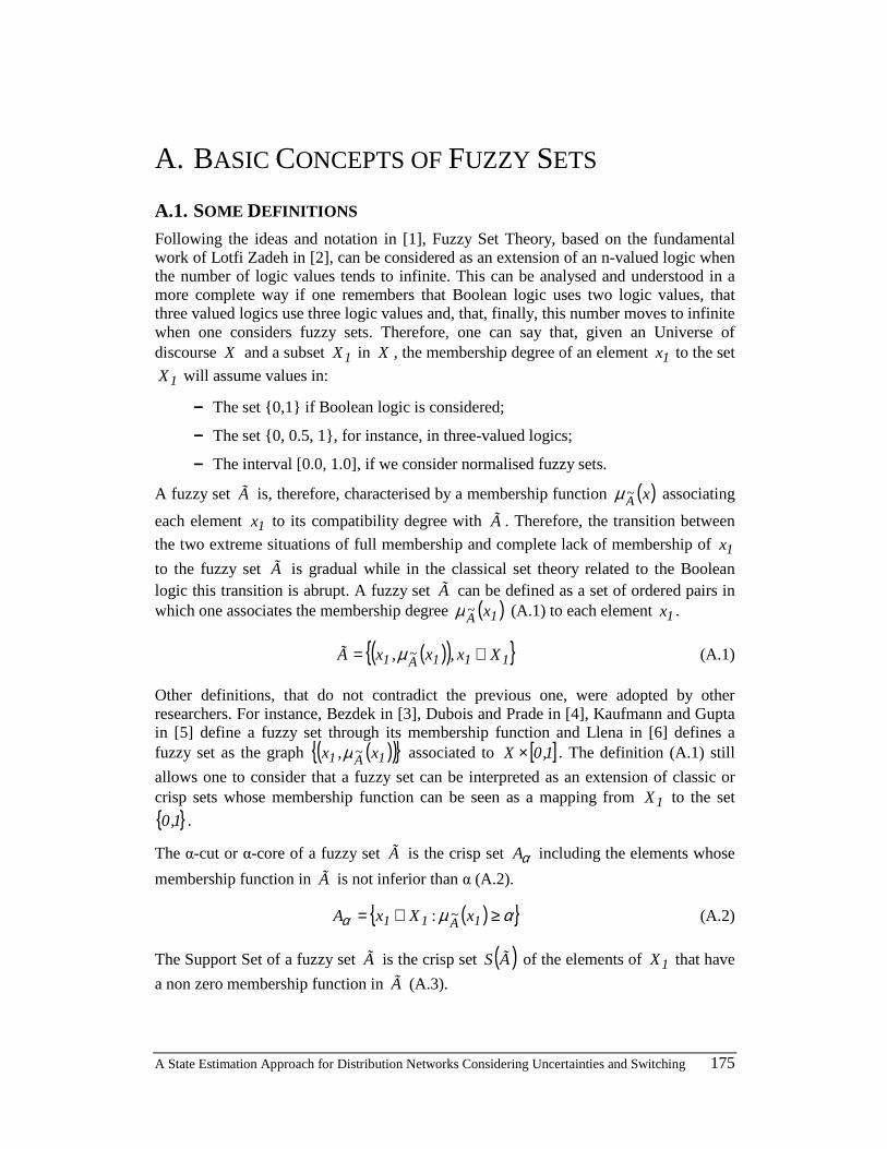
A State Estimation Approach for Distribution Networks Considering Uncertainties and Switching 175
A. BASIC CONCEPTS OF FUZZY SETS
A.1. SOME DEFINITIONS Following the ideas and notation in [1], Fuzzy Set Theory, based on the fundamental work of Lotfi Zadeh in [2], can be considered as an extension of an n-valued logic when the number of logic values tends to infinite. This can be analysed and understood in a more complete way if one remembers that Boolean logic uses two logic values, that three valued logics use three logic values and, that, finally, this number moves to infinite when one considers fuzzy sets. Therefore, one can say that, given an Universe of discourse X and a subset 1X in X , the membership degree of an element 1x to the set
1X will assume values in:
−−−− The set {0,1} if Boolean logic is considered;
−−−− The set {0, 0.5, 1}, for instance, in three-valued logics;
−−−− The interval [0.0, 1.0], if we consider normalised fuzzy sets.
A fuzzy set à is, therefore, characterised by a membership function ( )xA~µ associating
each element 1x to its compatibility degree with à . Therefore, the transition between
the two extreme situations of full membership and complete lack of membership of 1x
to the fuzzy set à is gradual while in the classical set theory related to the Boolean logic this transition is abrupt. A fuzzy set à can be defined as a set of ordered pairs in which one associates the membership degree ( )1A
~ xµ (A.1) to each element 1x .
( )( ){ }111A~1 Xx,x,xà ∈= µ (A.1)
Other definitions, that do not contradict the previous one, were adopted by other researchers. For instance, Bezdek in [3], Dubois and Prade in [4], Kaufmann and Gupta in [5] define a fuzzy set through its membership function and Llena in [6] defines a fuzzy set as the graph ( )( ){ }1A
~1 x,x µ associated to [ ]1,0X × . The definition (A.1) still
allows one to consider that a fuzzy set can be interpreted as an extension of classic or crisp sets whose membership function can be seen as a mapping from 1X to the set
{ }1,0 .
The α-cut or α-core of a fuzzy set à is the crisp set αA including the elements whose
membership function in à is not inferior than α (A.2).
( ){ }αµα ≥∈= 1A~11 xXxA : (A.2)
The Support Set of a fuzzy set à is the crisp set ( )ÃS of the elements of 1X that have
a non zero membership function in à (A.3).

Appendix A. Basic Concepts of Fuzzy Sets
176 A State Estimation Approach for Distribution Networks Considering Uncertainties and Switching
( ) ( ){ }0xXxÃS 1A~11 >∈= µ : (A.3)
A fuzzy set à is convex if and only if (A.4) holds. This definition means that, for any pair of values 1x and 2x , the membership degree of ix such that 2i1 xxx ≤≤ is non
inferior than the smaller of the membership degrees of 1x and 2x in à . Therefore, the fuzzy set sketched in the left side of the Figure A.1 is convex and the fuzzy set in the right side is not convex.
[ ] ( )( ) ( ) ( )( )2A~1A
~21A~121 x,xminx1xXx,x µµλλµλ ≥−+∈∀∈∀ ,0,1 , (A.4)
0 x
( )xA~µ
0 x
( )xA~µ
Figure A.1 – Membership functions for two fuzzy sets, one is convex (left function) and the other is non convex (right function).
A.2. BASIC OPERATIONS ON FUZZY SETS The membership function is a fundamental component of a fuzzy set so that several operations are usually defined through relations involving these functions. Zadeh in [2] proposed the following definitions for the union, intersection and complementation of fuzzy sets.
Let à and B~
be two fuzzy sets and let ( )xA~µ and ( )xB
~µ be their membership
functions. The membership functions of B~
à ∪ , B~
à ∩ and à are defined by (A.5), (A.6) and (A.7).
( ) ( ) ( ){ } Xx,x,xmaxx B~
A~
B~
A~ ∈=∪ µµµ (A.5)
( ) ( ) ( ){ } Xx,x,xminx B~
A~
B~
A~ ∈=∩ µµµ (A.6)
( ) ( ) Xx,x1x A~
A~ ∈−= µµ (A.7)
Considering, once again, the fuzzy sets à and B~
, the equality and inclusion relations are defined by (A.8) and (A.9).
( ) ( ) Xx,xx~~
B~
A~ ∈∀=⇔= µµBA (A.8)

A.3. Fuzzy Logic Operators
A State Estimation Approach for Distribution Networks Considering Uncertainties and Switching 177
( ) ( ) Xx,xx~~
B~
A~ ∈∀≥⇔⊇ µµBA (A.9)
Definitions (A.5), (A.6) and (A.7) allow one to clarify the fundamental difference between crisp sets and fuzzy sets. In Boolean logic, the Non-Contradiction and Excluded-Middle Laws hold. Considering the isomorphism between Boolean logic and Crisp Set Theory these two laws can be represented by (A.10) and (A.11).
∅=∩ AA (A.10)
XAA =∪ (A.11)
In Fuzzy Set Theory, these two laws are not valid. Considering the Non-Contradiction
Law, the degree of membership of x in A~
A~ ∩ , according to (A.6) and (A.7), is given
by (A.12) or, in an equivalent way, by (A.13). This way, one can conclude that an element x can have simultaneously non zero membership degrees to a fuzzy set and to its complementary.
( ) ( ) ( ){ } Xx,x1,xminx A~
A~
ÃÃ∈−=∩ µµµ (A.12)
( ) ( ) ( ) ( ) ( )( ) ( ) ( ) ( ) Xx,
5.0xx1xif,x1
5.0xx1xif,xx
A~
A~
A~
A~
A~
A~
A~
A~
ÃÃ∈
≥⇔−≥−≤⇔−≤
=∩ µµµµµµµµ
µ (A.13)
Regarding the Excluded Middle Law, according to (A.5) and (A.7), the degree of
membership of x in A~
A~ ∪ is given by (A.14). This means that the union of a fuzzy set
with its complementary may not have as a result the universe X .
( ) ( ) ( ) ( ) ( )( ) ( ) ( ) ( ) Xx,
5.0xx1xif,x1
5.0xx1xif,xx
A~
A~
A~
A~
A~
A~
A~
A~
ÃÃ∈
≤⇔−≤−≥⇔−≥
=∪ µµµµµµµµ
µ (A.14)
A.3. FUZZY LOGIC OPERATORS
A.3.1. T-NORMS AND T-CONORMS
The definitions of the union (based on max operator), intersection (based on min operator) and complementation proposed by Zadeh in [2] were re-established afterwards by Bellman and Giertz. These researchers formulated a set of axioms, referred by Zimmermann in [7] and by El-Hawary in [8]. They also proved that the operators given by (A.5), (A.6) and (A.7) are the only ones to be in accordance with those axioms.
Until now, the minimum operator was used to represent the intersection of fuzzy sets, interpreted as the logical “and”. Moreover, the maximum operator was used to represent the union, interpreted as the logical “or”. Alternative operators were also proposed as described in [8]. These proposals vary with respect to the generality or adaptability of the operators as well as to the degree to which and how they are justified. The way in which this justification was handled ranges from intuitive arguments to empirical or
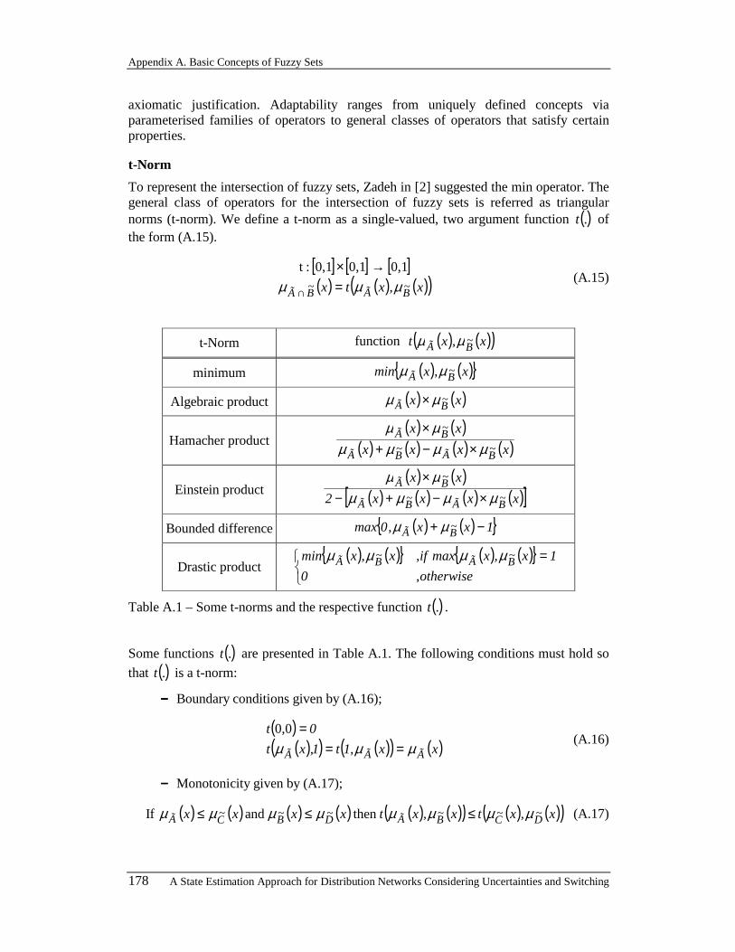
Appendix A. Basic Concepts of Fuzzy Sets
178 A State Estimation Approach for Distribution Networks Considering Uncertainties and Switching
axiomatic justification. Adaptability ranges from uniquely defined concepts via parameterised families of operators to general classes of operators that satisfy certain properties.
t-Norm
To represent the intersection of fuzzy sets, Zadeh in [2] suggested the min operator. The general class of operators for the intersection of fuzzy sets is referred as triangular norms (t-norm). We define a t-norm as a single-valued, two argument function ( ).t of the form (A.15).
[ ] [ ] [ ]( ) ( ) ( )( )x,xtx B
~ÃB~
à µµµ =→×
∩
0,10,10,1:t (A.15)
t-Norm function ( ) ( )( )x,xt B~Ã µµ
minimum ( ) ( ){ }x,xmin B~Ã µµ
Algebraic product ( ) ( )xx B~Ã µµ ×
Hamacher product ( ) ( )
( ) ( ) ( ) ( )xxxx
xx
B~ÃB
~Ã
B~Ã
µµµµµµ
×−+×
Einstein product ( ) ( )
( ) ( ) ( ) ( )[ ]xxxx2
xx
B~ÃB
~Ã
B~Ã
µµµµµµ
×−+−×
Bounded difference ( ) ( ){ }1xx,0max B~Ã −+ µµ
Drastic product ( ) ( ){ } ( ) ( ){ }
=
otherwise,0
1x,xmaxif,x,xmin B~ÃB
~Ã µµµµ
Table A.1 – Some t-norms and the respective function ( ).t .
Some functions ( ).t are presented in Table A.1. The following conditions must hold so
that ( ).t is a t-norm:
−−−− Boundary conditions given by (A.16);
( )( )( ) ( )( ) ( )xx,1t1,xt
0t
ÃÃÃ µµµ ===
0,0 (A.16)
−−−− Monotonicity given by (A.17);
( ) ( ) ( ) ( ) ( ) ( )( ) ( ) ( )( )x,xtx,xtxxxx D~
C~
B~ÃD
~B~
C~Ã µµµµµµµµ then and If ≤≤≤ (A.17)
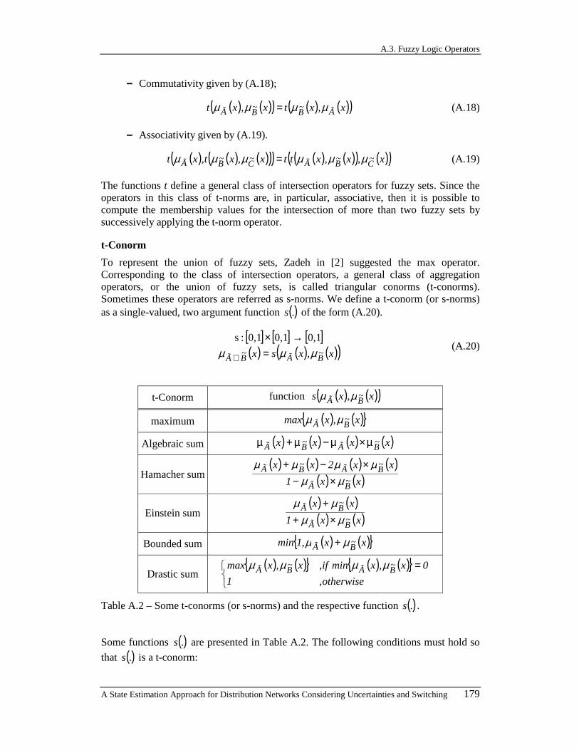
A.3. Fuzzy Logic Operators
A State Estimation Approach for Distribution Networks Considering Uncertainties and Switching 179
−−−− Commutativity given by (A.18);
( ) ( )( ) ( ) ( )( )x,xtx,xt ÃB~
B~Ã µµµµ = (A.18)
−−−− Associativity given by (A.19).
( ) ( ) ( )( )( ) ( ) ( )( ) ( )( )x,x,xttx,xt,xt C~
B~ÃC
~B~Ã µµµµµµ = (A.19)
The functions t define a general class of intersection operators for fuzzy sets. Since the operators in this class of t-norms are, in particular, associative, then it is possible to compute the membership values for the intersection of more than two fuzzy sets by successively applying the t-norm operator.
t-Conorm
To represent the union of fuzzy sets, Zadeh in [2] suggested the max operator. Corresponding to the class of intersection operators, a general class of aggregation operators, or the union of fuzzy sets, is called triangular conorms (t-conorms). Sometimes these operators are referred as s-norms. We define a t-conorm (or s-norms) as a single-valued, two argument function ( ).s of the form (A.20).
[ ] [ ] [ ]( ) ( ) ( )( )x,xsx B
~ÃB~
à µµµ =→×
∪
0,10,10,1:s (A.20)
t-Conorm function ( ) ( )( )x,xs B~Ã µµ
maximum ( ) ( ){ }x,xmax B~Ã µµ
Algebraic sum ( ) ( ) ( ) ( )xxxx B~ÃB
~Ã µ×µ−µ+µ
Hamacher sum ( ) ( ) ( ) ( )
( ) ( )xx1
xx2xx
B~Ã
B~ÃB
~Ã
µµµµµµ
×−×−+
Einstein sum ( ) ( )
( ) ( )xx1
xx
B~Ã
B~Ã
µµµµ×+
+
Bounded sum ( ) ( ){ }xx,1min B~Ã µµ +
Drastic sum ( ) ( ){ } ( ) ( ){ }
=
otherwise,1
0x,xminif,x,xmax B~ÃB
~Ã µµµµ
Table A.2 – Some t-conorms (or s-norms) and the respective function ( ).s .
Some functions ( ).s are presented in Table A.2. The following conditions must hold so
that ( ).s is a t-conorm:

Appendix A. Basic Concepts of Fuzzy Sets
180 A State Estimation Approach for Distribution Networks Considering Uncertainties and Switching
−−−− Boundary conditions given by (A.21);
( )( )( ) ( )( ) ( )xx,0s0,xs
1s
ÃÃÃ µµµ ===
1,1 (A.21)
−−−− Monotonicity given by (A.22);
( ) ( ) ( ) ( ) ( ) ( )( ) ( ) ( )( )x,xsx,xsxxxx D~
C~
B~ÃD
~B~
C~Ã µµµµµµµµ then and If ≤≤≤ (A.22)
−−−− Commutativity given by (A.23);
( ) ( )( ) ( ) ( )( )x,xsx,xs ÃB~
B~Ã µµµµ = (A.23)
−−−− Associativity given by (A.24).
( ) ( ) ( )( )( ) ( ) ( )( ) ( )( )x,x,xssx,xs,xs C~
B~ÃC
~B~Ã µµµµµµ = (A.24)
t-norms and t-conorms are related in a sense of logical duality. A t-conorm can be defined as a two-argument function mapping from [ ] [ ]0,10,1 × to [ ]0,1 , such that the function t defined as (A.25) is a t-norm. Therefore, any t-conorm can be generated from a t-norm t through this transformation. More generally, for suitable negation operators like the complement operator for fuzzy sets, defined by (A.7), pairs of t-norms t and t-conorms s satisfy the generalization of De Morgan’s law (A.26).
( ) ( )( ) ( ) ( )( )x1,x1s1x,xt B~ÃB
~Ã µµµµ −−−= (A.25)
( ) ( )( ) ( ) ( )( )( ) ( )( ) ( ) ( )( )x,xt1x,xs
x,xs1x,xt
B~ÃB
~Ã
B~ÃB
~Ã
µµµµ
µµµµ
−=
−= (A.26)
Typical pairs of t-norms and t-conorms are displayed in Table A.3. The t-norms in this table are the ones included in Table A.1 and the t-conorms are the ones in Table A.2.
t-Norm t-Conorm
minimum maximum
Algebraic product Algebraic sum
Hamacher product Hamacher sum
Einstein product Einstein sum
Bounded difference Bounded sum
Drastic product Drastic sum
Table A.3 – Typical dual pairs of t-norms and t-conorms (or s-norms).

A.3. Fuzzy Logic Operators
A State Estimation Approach for Distribution Networks Considering Uncertainties and Switching 181
However, the t-norms and t-conorms for the union and intersection operations are not the only ones, as other sets of axioms were proposed by other researchers. In this scope, El-Hawary in [8] presents several other families of aggregation operators as the Hamacher’s family, Yager’s family, Dubois and Prade’s family, Schweizer and Sklar’s family, Dombi’s family, Frank’s family. They are also presented the axioms related to the Hamacher operator.
A.3.2. SELECTION OF THE AGGREGATION OPERATORS TO BE USED
The selection of operators to be used to aggregate fuzzy sets has a great importance if one remembers that Fuzzy Set Theory is not a purely formal theory but it also aims at modeling real phenomena. Therefore, the representation of the world through Fuzzy Set Theory should not be the cause of large distortions of the phenomena being analysed. This turns into an even more delicate question knowing that fuzzy sets can be used to build mathematical representations of propositions of human natural language so that they can be integrated in subsequent calculations. For this reason one should use the operators that represent more adequately the different phases of human reasoning. That is why purely axiomatic justifications may not be enough.
In this scope, Thöle, Zimmermann and Zysno in [9] analysed, in an experimental way, the adequacy of the minimum and algebraic product to model the intersection of fuzzy sets. For this purpose, they used the answers of a set of students of a German university to a pre-established set of questions. From the results, they concluded that the membership function of the intersection can be larger than the minimum value of the membership functions of the elements to be aggregated. In the conclusions of this research, it was also referred that none of the two studied operators are able to perform the intersection in a fully adequate way. Nevertheless, it seems that the minimum operator should be preferred. On the other hand, in [10] Turksen describes in a detailed way, a set of methodologies to be used to measure and build membership functions requiring different levels of data discrimination.
Several criteria have been referred to be used to select the operators on fuzzy sets. Among them, one can refer:
−−−− Axiomatic strength;
−−−− Experimental adequacy;
−−−− Adaptability;
−−−− Numerical efficiency;
−−−− Degree of compensation;
−−−− Range of values that the resulting membership function can assume;
−−−− Behavior of the aggregation process;
−−−− Discrimination level required to the membership functions to be aggregated.
The two first criteria of this list have a formal and an experimental nature, respectively, while the other ones have a pragmatic character. A detailed description of these criteria can be found in Zimmermann [11].

Appendix A. Basic Concepts of Fuzzy Sets
182 A State Estimation Approach for Distribution Networks Considering Uncertainties and Switching
A.4. FUZZY NUMBERS A fuzzy number is defined as a normalized, convex fuzzy set defined on the real axis such that its membership function is piece wise continuous. A fuzzy number à is positive or negative if (A.27) or (A.28) hold, respectively. If (A.29) holds the number is non negative. It is a non positive number if (A.30) holds.
( ) 0x,0xA~ ≤∀=µ (A.27)
( ) 0x,0xA~ ≥∀=µ (A.28)
( ) 0x,0xA~ <∀=µ (A.29)
( ) 0x,0xA~ >∀=µ (A.30)
Among the several types of fuzzy numbers, one will address in the next paragraphs triangular, trapezoidal, Gaussian and L-R fuzzy numbers.
A.4.1. TRIANGULAR FUZZY NUMBER
The membership function of a triangular fuzzy number à can be represented by (A.31). Therefore, the α-cut ( ∈α [0,1]) of this fuzzy number is given by (A.32). A number of this type, as the one sketched in Figure A.2, can be used to represent the uncertain knowledge about a value 2a admitting that values in ] [ ] [3221 a,aa,a ∪ are still possible representations of this value having, however, lower compatibility degrees than the one of 2a . In a symbolic way one can represent a number of this type by ( )321 a,a,a .
( )
[ ]
[ ]
[ ]
∉
∈−
−
∈−
−
=
31
3232
3
2112
1
A~
a,axif,0
a,axif,aa
ax
a,axif,aa
ax
xµ (A.31)
( ) ( )[ ]323121 aaa,aaaA −+−+= ααα (A.32)

A.4. Fuzzy Numbers
A State Estimation Approach for Distribution Networks Considering Uncertainties and Switching 183
0
1
x
( )xA~µ
2a1a 3a
Figure A.2 – Membership function for a triangular fuzzy number.
A.4.2. TRAPEZOIDAL FUZZY NUMBER
If a trapezoidal fuzzy number à is considered, the membership function is given by (A.33). Therefore, the α-cut ( ∈α [0,1]) of this fuzzy number is given by (A.34). A number of this type can be used to model the uncertainty around [ ]32 a,a . In this sense, the values in this interval have a membership value of 1.0 indicating that they are equally good representations of that knowledge having, therefore, maximum credibility. The values in ] [ ] [4321 a,aa,a ∪ are still possible representations but having lower
levels of credibility. In Figure A.3 one sketches a trapezoidal fuzzy number. In a symbolic way one can represent a number of this type by ( )4321 a,a,a,a . This fuzzy
number degenerates in a triangular fuzzy number if 32 aa = . On the other hand, a
trapezoidal fuzzy number degenerates in a rectangular one if 21 aa = and 43 aa = ,
which corresponds to a crisp set.
( )
[ ][ ][ ][ ]
∉
∈−−
∈
∈−
−
=
41
4343
4
32
2112
1
A~
a,axif,0
a,axif,aa
axa,axif,1
a,axif,aa
ax
xµ (A.33)
( ) ( )[ ]434121 aaa,aaaA −+−+= ααα (A.34)
0
1
x
( )xA~µ
2a1a 3a 4a Figure A.3 – Membership function for a trapezoidal fuzzy number.

Appendix A. Basic Concepts of Fuzzy Sets
184 A State Estimation Approach for Distribution Networks Considering Uncertainties and Switching
A.4.3. GAUSSIAN FUZZY NUMBER
If a Gaussian fuzzy number à is considered, the membership function is given by (A.35). Therefore, the α-cut ( ∈α [0,1]) of this fuzzy number is given by (A.36). A number of this type can be used to model the uncertainty around m, which is a parameter of this function and it corresponds to the point regarding which the function is symmetrical. Another parameter of this function is d that represents the spread or the width of the membership function. This parameter has a value that is always positive. In Figure A.4 one sketches a Gaussian fuzzy number.
( )2
d
mx
A~ ex
−−
=µ (A.35)
[ ]ααα ee logdm,logdmA −+−−= (A.36)
0
.3679
1
m x
( )xA~µ
m+dm-d
Figure A.4 – Membership function for a Gaussian fuzzy number.
A.4.4. LR FUZZY NUMBER
Dubois and Prade in [12] suggested a new type of fuzzy numbers, the LR fuzzy numbers. These numbers are defined using functions, called reference ones, having the following properties:
−−−− They are symmetrical regarding the zero, ( ) ( )xfxf −= ;
−−−− For zero they have a value equal to one, ( ) 0.10f = ;
−−−− They are decreasing functions in [0,+∞[.
Using functions L and R having these properties, these authors defined a LR fuzzy number as a fuzzy number whose membership function is given by (A.37). In a symbolic way, such a number can be represented by (A.38).
( )
>≥
−
>≤
−
=0andmxif,
mxR
0andmxif,xm
L
xA~
ββ
ααµ (A.37)
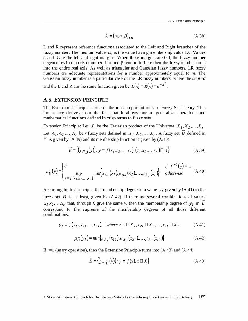
A.5. Extension Principle
A State Estimation Approach for Distribution Networks Considering Uncertainties and Switching 185
( )LR,,mà βα= (A.38)
L and R represent reference functions associated to the Left and Right branches of the fuzzy number. The medium value, m, is the value having membership value 1.0. Values α and β are the left and right margins. When these margins are 0.0, the fuzzy number degenerates into a crisp number. If α and β tend to infinite then the fuzzy number turns into the entire real axis. As well as triangular and Gaussian fuzzy numbers, LR fuzzy numbers are adequate representations for a number approximately equal to m. The Gaussian fuzzy number is a particular case of the LR fuzzy numbers, where the α=β=d
and the L and R are the same function given by ( ) ( ) 2xexRxL −== .
A.5. EXTENSION PRINCIPLE The Extension Principle is one of the most important ones of Fuzzy Set Theory. This importance derives from the fact that it allows one to generalize operations and mathematical functions defined in crisp terms to fuzzy sets.
Extension Principle: Let X be the Cartesian product of the Universes r21 X,,X,X K .
Let r21 Ã,,Ã,Ã K be r fuzzy sets defined in r21 X,,X,X K . A fuzzy set B~
defined in Y is given by (A.39) and its membership function is given by (A.40).
( )( ) ( ) ( ){ }X,x,,xx,,x,,xxf: yyy,µB~
r21r21B~ ∈== KK (A.39)
( )( )
( )( ) ( ) ( ){ }
∅=
==
−
otherwise,xµ,,xµ,xµminsup
yfif,0yµ
rÃ2Ã1Ã,x,,xxfy
1
B~
r21r21
KK
(A.40)
According to this principle, the membership degree of a value 1y given by (A.41) to the
fuzzy set B~
is, at least, given by (A.42). If there are several combinations of values
r21 ,x,,xx K that, through f, give the same y, then the membership degree of 1y in B~
correspond to the supreme of the membership degrees of all those different combinations.
( ) r1r2211111r21111 Xx,,Xx,Xxwhere,,x,,xxfy ∈∈∈= KK (A.41)
( ) ( ) ( ) ( ){ }1rÃ21Ã11Ã1B~ xµ,,xµ,xµminyµ
r21K= (A.42)
If r=1 (unary operation), then the Extension Principle turns into (A.43) and (A.44).
( )( ) ( ){ }Xx,xf: yyy,µB~
B~ ∈== (A.43)
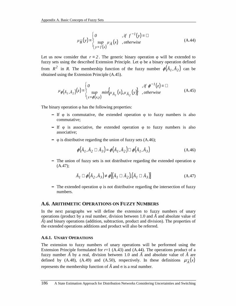
Appendix A. Basic Concepts of Fuzzy Sets
186 A State Estimation Approach for Distribution Networks Considering Uncertainties and Switching
( )( )
( )( )
∅=
==
−
otherwise,xµsup
yfif,0yµ
Ãxfy
1
B~ (A.44)
Let us now consider that 2r = . The generic binary operation φ will be extended to fuzzy sets using the described Extension Principle. Let φ be a binary operation defined
from 2R in R. The membership function of the fuzzy number ( )21 Ã,Ãϕ can be obtained using the Extension Principle (A.45).
( )( )( )
( )( ) ( ){ }
∅=
==
−
otherwise,yµ,xµminsup
zif,0zµ
2121 ÃÃ
x,yz
1
Ã,Ãϕ
ϕϕ
(A.45)
The binary operation φ has the following properties:
−−−− If φ is commutative, the extended operation φ to fuzzy numbers is also commutative;
−−−− If φ is associative, the extended operation φ to fuzzy numbers is also associative;
−−−− φ is distributive regarding the union of fuzzy sets (A.46);
( ) ( ) ( )3121321 Ã,ÃÃ,ÃÃÃ,Ã ϕϕϕ ∪=∪ (A.46)
−−−− The union of fuzzy sets is not distributive regarding the extended operation φ (A.47);
( ) ( ) ( )[ ]3121321 ÃÃ,ÃÃÃ,ÃÃ ∪∪≠∪ ϕϕ (A.47)
−−−− The extended operation φ is not distributive regarding the intersection of fuzzy numbers.
A.6. ARITHMETIC OPERATIONS ON FUZZY NUMBERS In the next paragraphs we will define the extension to fuzzy numbers of unary operations (product by a real number, division between 1.0 and à and absolute value of Ã) and binary operations (addition, subtraction, product and division). The properties of the extended operations additions and product will also be referred.
A.6.1. UNARY OPERATIONS
The extension to fuzzy numbers of unary operations will be performed using the Extension Principle formulated for r=1 (A.43) and (A.44). The operations product of a fuzzy number à by a real, division between 1.0 and à and absolute value of à are defined by (A.48), (A.49) and (A.50), respectively. In these definitions ( )xA
~µ
represents the membership function of à and σ is a real number.

A.6. Arithmetic Operations on Fuzzy Numbers
A State Estimation Approach for Distribution Networks Considering Uncertainties and Switching 187
( ) 0,xµxµ ÃÃ ≠∀
= σσσ (A.48)
( ) 0x,x
0.1µxµ ÃÃ 1 ≠∀
=− (A.49)
( ) ( ) ( )( )
<≥−
=0xif,0
0xif,xµ,xµmaxyµ ÃÃ
à (A.50)
According to these definitions one can say that:
−−−− The product of a fuzzy number by a real number σ is distributive regarding the addition of fuzzy numbers (A.51). However, the distributive property of the product of a fuzzy number by a real σ regarding the addition of real numbers does not hold (A.52);
( ) ( ) ( )2121 ÃÃÃÃ σσσ ⊕=⊕ (A.51)
( ) ( ) ( )ÃÃÃ 2121 σσσσ ⊕≠+ (A.52)
−−−− If the fuzzy number à is not non positive or is not non negative then result of the division between 1.0 and à is not convex and, thus, is not a fuzzy number;
−−−− The fuzzy number related to the absolute value of à is non negative.
A.6.2. BINARY OPERATIONS
The extension to fuzzy numbers of binary operations will be performed using the Extension Principle formulated for r=2 (A.45).
Addition
The binary operation addition ( ) 2121 ÃÃÃ,Ã ⊕=ϕ is a fuzzy number whose membership function is given by (A.53).
( ) ( ) ( ){ }yµ,xµminsupzµ2121 ÃÃ
yxzÃÃ
+=⊕ = (A.53)
This extended operation has the following properties:
−−−− Commutativity;
−−−− Associativity;
−−−− It holds the equality: ( ) ( ) ( )2121 ÃÃÃÃ −⊕−=⊕− ;
−−−− The crisp number 0.0 is the neutral element of the extended addition, that is,
111 Ã,Ã0Ã ∀=⊕ .

Appendix A. Basic Concepts of Fuzzy Sets
188 A State Estimation Approach for Distribution Networks Considering Uncertainties and Switching
−−−− Given a fuzzy number, there is not another fuzzy number that added with the first one gives 0.0. In this sense, no fuzzy number has opposite regarding the extended addition. Thus, the set of fuzzy numbers associated with this operation is not a group.
Subtraction
The binary operation subtraction can be redefined considering (A.54). Therefore, using the Extension Principle, one can obtain (A.55).
( )2121 ÃÃÃÃ −⊕=Θ (A.54)
( ) ( ) ( ){ }yµ,xµminsupzµ2121 ÃÃ
yxzÃÃ −
+==Θ (A.55)
Product
The product of two fuzzy numbers both non negative or both non positive, 21 ÃÃ ⊗ , is a fuzzy number. Its membership function, according to the Extension Principle, is given by (A.56). Considering (A.56), the product of two both negative or positive fuzzy numbers is a positive fuzzy number.
( ) ( ) ( ){ }yµ,xµminsupzµ2121 ÃÃ
yxzÃÃ
×=⊗ = (A.56)
In a similar way to what we have done for the extended subtraction, the product of a non positive by a non negative number, can be redefined according to (A.57).
( )( )2121 ÃÃÃÃ ⊗−−=⊗ (A.57)
This extended operation has the following properties:
−−−− Commutativity;
−−−− Associativity;
−−−− It holds the equality: ( ) ( ) ( )2121 ÃÃÃÃ ⊗−=⊗− ;
−−−− The crisp number 1.0 is the neutral element of the extended product. This means that, 111 Ã,Ã1Ã ∀=⊗ ;
−−−− Given a fuzzy number Ã, there is no other fuzzy number that, if multiplied by Ã, gives 1.0. In this sense, no fuzzy number has opposite regarding the extended product. Therefore, the set of fuzzy numbers associated to this operation is not a group.
Division
If 1Ã and 2Ã are respectively non negative and positive (or non positive and negative) fuzzy numbers, the binary operation division can be redefined by (A.58). Now, using the Extension Principle we can obtain (A.59).
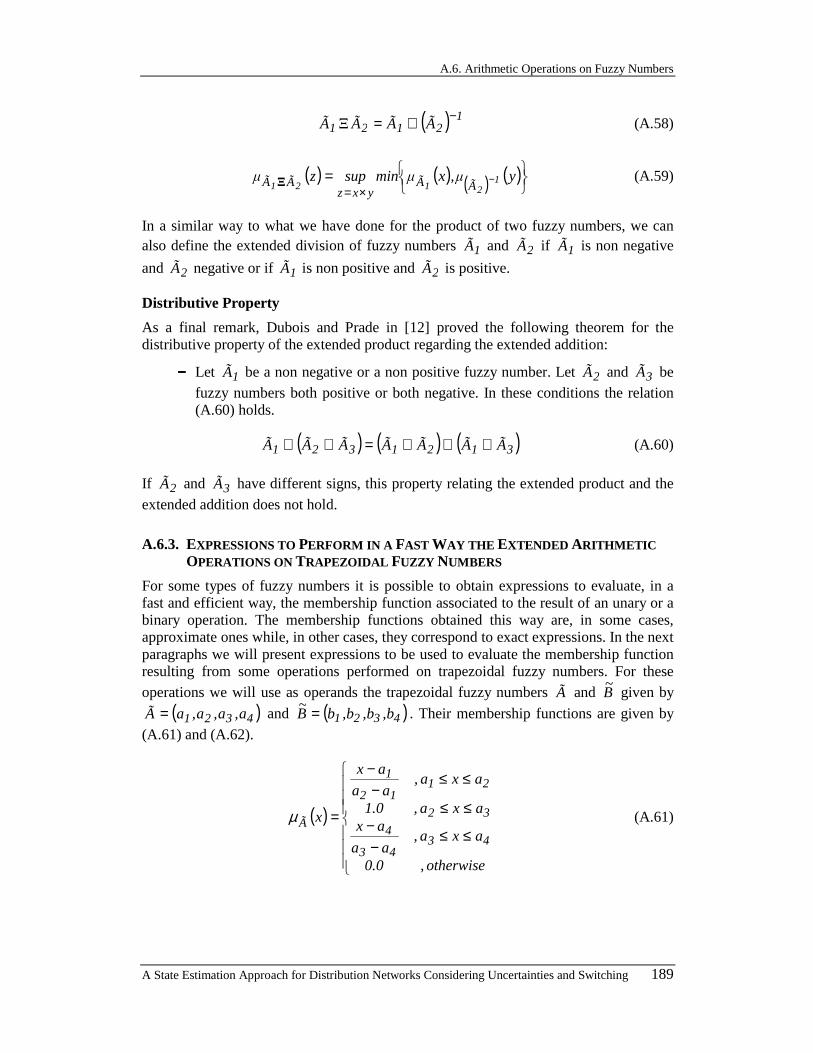
A.6. Arithmetic Operations on Fuzzy Numbers
A State Estimation Approach for Distribution Networks Considering Uncertainties and Switching 189
( ) 12121 ÃÃÃÃ
−⊗=Ξ (A.58)
( ) ( ) ( ) ( )
= −
×=yµ,xµminsupzµ 1
2121 ÃÃyxz
ÃÃ Ξ (A.59)
In a similar way to what we have done for the product of two fuzzy numbers, we can also define the extended division of fuzzy numbers 1Ã and 2Ã if 1Ã is non negative
and 2Ã negative or if 1Ã is non positive and 2Ã is positive.
Distributive Property
As a final remark, Dubois and Prade in [12] proved the following theorem for the distributive property of the extended product regarding the extended addition:
−−−− Let 1Ã be a non negative or a non positive fuzzy number. Let 2Ã and 3Ã be fuzzy numbers both positive or both negative. In these conditions the relation (A.60) holds.
( ) ( ) ( )3121321 ÃÃÃÃÃÃÃ ⊗⊕⊗=⊕⊗ (A.60)
If 2Ã and 3Ã have different signs, this property relating the extended product and the
extended addition does not hold.
A.6.3. EXPRESSIONS TO PERFORM IN A FAST WAY THE EXTENDED ARITHMETIC OPERATIONS ON TRAPEZOIDAL FUZZY NUMBERS
For some types of fuzzy numbers it is possible to obtain expressions to evaluate, in a fast and efficient way, the membership function associated to the result of an unary or a binary operation. The membership functions obtained this way are, in some cases, approximate ones while, in other cases, they correspond to exact expressions. In the next paragraphs we will present expressions to be used to evaluate the membership function resulting from some operations performed on trapezoidal fuzzy numbers. For these operations we will use as operands the trapezoidal fuzzy numbers à and B
~ given by
( )4321 a,a,a,aà = and ( )4321 b,b,b,bB~ = . Their membership functions are given by
(A.61) and (A.62).
( )
≤≤−−
≤≤
≤≤−
−
=
otherwise,0.0
axa,aa
axaxa,0.1
axa,aa
ax
x
4343
4
32
2112
1
õ (A.61)
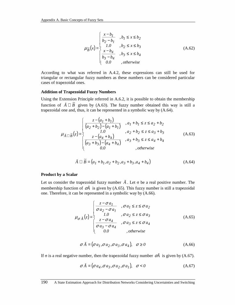
Appendix A. Basic Concepts of Fuzzy Sets
190 A State Estimation Approach for Distribution Networks Considering Uncertainties and Switching
( )
≤≤−−
≤≤
≤≤−−
=
otherwise,0.0
bxb,bb
bxbxb,0.1
bxb,bb
bx
x
4343
4
32
2112
1
B~µ (A.62)
According to what was referred in A.4.2, these expressions can still be used for triangular or rectangular fuzzy numbers as these numbers can be considered particular cases of trapezoidal ones.
Addition of Trapezoidal Fuzzy Numbers
Using the Extension Principle referred in A.6.2, it is possible to obtain the membership
function of B~
à ⊕ given by (A.63). The fuzzy number obtained this way is still a trapezoidal one and, thus, it can be represented in a symbolic way by (A.64).
( )
( )( ) ( )
( )( ) ( )
+≤≤++−+
+−+≤≤+
+≤≤++−+
+−
=⊕
otherwise,0.0
bazba,baba
bazbazba,0.1
bazba,baba
baz
z
44334433
44
3322
22111122
11
B~
õ (A.63)
( )44332211 ba,ba,ba,baB~
à ++++=⊕ (A.64)
Product by a Scalar
Let us consider the trapezoidal fuzzy number à . Let σ be a real positive number. The membership function of Ãσ is given by (A.65). This fuzzy number is still a trapezoidal one. Therefore, it can be represented in a symbolic way by (A.66).
( )
≤≤−
−≤≤
≤≤−
−
=
otherwise,0.0
aza,aa
azaza,0.1
aza,aa
az
z
4343
4
32
2112
1
Ãσσ
σσσ
σσ
σσσσ
σ
µσ (A.65)
( ) 0,a,a,a,aà 4321 ≥= σσσσσσ (A.66)
If σ is a real negative number, then the trapezoidal fuzzy number Ãσ is given by (A.67).
( ) 0,a,a,a,aà 1234 <= σσσσσσ (A.67)

A.6. Arithmetic Operations on Fuzzy Numbers
A State Estimation Approach for Distribution Networks Considering Uncertainties and Switching 191
Subtraction of Two Trapezoidal Fuzzy Numbers
Let us consider, once again, the two trapezoidal fuzzy numbers à and B~
. According to what was referred in A.6.2, the binary operation subtraction can be performed considering (A.68) and the expression obtained to perform the addition of two fuzzy numbers and the product of a fuzzy number by the scalar σ=-1.0. Therefore, the
membership function of B~
ÃΘ is given by (A.69). This still corresponds to a trapezoidal fuzzy number and, thus, it can be represented by (A.70).
( )B~
0.1ÃB~
à ×−⊕=Θ (A.68)
( )
( )( ) ( )
( )( ) ( )
−≤≤−−−−
−−−≤≤−
−≤≤−−−−
−−
=
otherwise,0.0
bazba,baba
bazbazba,0.1
bazba,baba
baz
z
14231423
14
2332
32414132
41
B~
ÃΘµ (A.69)
( )14233241 ba,ba,ba,baB~
à −−−−=Θ (A.70)
Product of Two Trapezoidal Fuzzy Numbers
The product of two trapezoidal fuzzy numbers is not, in general, a fuzzy number of this type. In fact, it is possible to prove that the left and right branches of the membership
function of B~
à ⊗ correspond to concave and convex curves, respectively, assuming
that à and B~
are both non positive or non negative numbers. This non linear character
is due to the presence of quadratic terms in the membership function of B~
à ⊗ . If, among others, these non linear terms are not considered, the exact expression of the membership function degenerates in the membership function of a trapezoidal fuzzy number. In the majority of the current life situations this trapezoidal approximation is sufficient.
If à and B~
are two both non negative trapezoidal numbers the operation product
B~
à ⊗ has a membership function approximated by a trapezoidal fuzzy number given by (A.71). This number can be symbolically represented by (A.72).
( )
≤≤−
−≤≤
≤≤−
−
≅⊗
otherwise,0.0
bazba,baba
bazbazba,0.1
bazba,baba
baz
z
44334433
44
3322
22111122
11
B~
õ (A.71)
( )44332211 ba,ba,ba,baB~
à ≅⊗ (A.72)
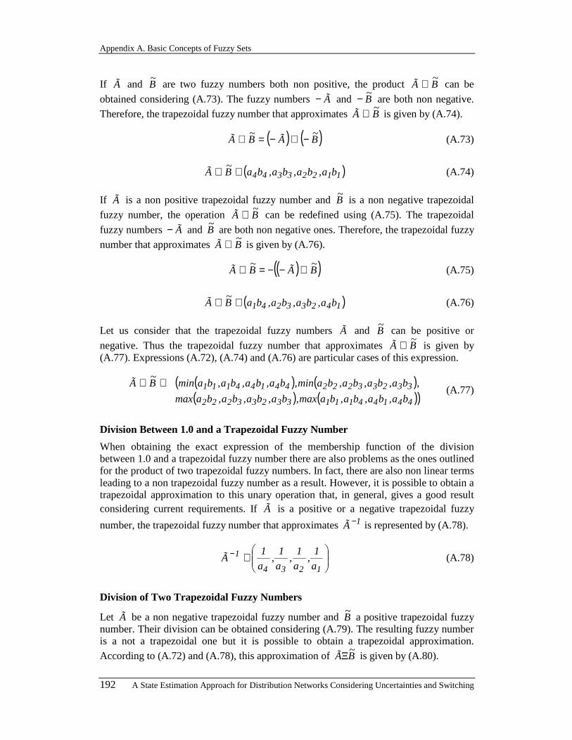
Appendix A. Basic Concepts of Fuzzy Sets
192 A State Estimation Approach for Distribution Networks Considering Uncertainties and Switching
If à and B~
are two fuzzy numbers both non positive, the product B~
à ⊗ can be
obtained considering (A.73). The fuzzy numbers Ã− and B~− are both non negative.
Therefore, the trapezoidal fuzzy number that approximates B~
à ⊗ is given by (A.74).
( ) ( )B~
ÃB~
à −⊗−=⊗ (A.73)
( )11223344 ba,ba,ba,baB~
à ≅⊗ (A.74)
If à is a non positive trapezoidal fuzzy number and B~
is a non negative trapezoidal
fuzzy number, the operation B~
à ⊗ can be redefined using (A.75). The trapezoidal
fuzzy numbers Ã− and B~
are both non negative ones. Therefore, the trapezoidal fuzzy
number that approximates B~
à ⊗ is given by (A.76).
( )( )B~
ÃB~
à ⊗−−=⊗ (A.75)
( )14233241 ba,ba,ba,baB~
à ≅⊗ (A.76)
Let us consider that the trapezoidal fuzzy numbers à and B~
can be positive or
negative. Thus the trapezoidal fuzzy number that approximates B~
à ⊗ is given by (A.77). Expressions (A.72), (A.74) and (A.76) are particular cases of this expression.
( ) ( )(( ) ( ))4414411133233222
3323322244144111
ba,ba,ba,bamax,ba,ba,ba,bamax
,ba,ba,ba,bamin,ba,ba,ba,baminB~
à ≅⊗ (A.77)
Division Between 1.0 and a Trapezoidal Fuzzy Number
When obtaining the exact expression of the membership function of the division between 1.0 and a trapezoidal fuzzy number there are also problems as the ones outlined for the product of two trapezoidal fuzzy numbers. In fact, there are also non linear terms leading to a non trapezoidal fuzzy number as a result. However, it is possible to obtain a trapezoidal approximation to this unary operation that, in general, gives a good result considering current requirements. If à is a positive or a negative trapezoidal fuzzy
number, the trapezoidal fuzzy number that approximates 1Ã − is represented by (A.78).
≅−
1234
1
a
1,
a
1,
a
1,
a
1Ã (A.78)
Division of Two Trapezoidal Fuzzy Numbers
Let à be a non negative trapezoidal fuzzy number and B~
a positive trapezoidal fuzzy number. Their division can be obtained considering (A.79). The resulting fuzzy number is a not a trapezoidal one but it is possible to obtain a trapezoidal approximation.
According to (A.72) and (A.78), this approximation of B~
ÃΞ is given by (A.80).
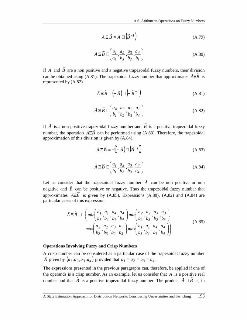
A.6. Arithmetic Operations on Fuzzy Numbers
A State Estimation Approach for Distribution Networks Considering Uncertainties and Switching 193
( )1B~
ÃB~
à −⊗=Ξ (A.79)
≅
1
4
2
3
3
2
4
1
b
a,
b
a,
b
a,
b
aB~
Ã Ξ (A.80)
If à and B~
are a non positive and a negative trapezoidal fuzzy numbers, their division can be obtained using (A.81). The trapezoidal fuzzy number that approximates B
~ÃΞ is
represented by (A.82).
( ) ( )1B~
ÃB~
à −−⊗−=Ξ (A.81)
≅
4
1
3
2
2
3
1
4
b
a,
b
a,
b
a,
b
aB~
Ã Ξ (A.82)
If à is a non positive trapezoidal fuzzy number and B~
is a positive trapezoidal fuzzy number, the operation B
~ÃΞ can be performed using (A.83). Therefore, the trapezoidal
approximation of this division is given by (A.84).
( ) ( )( )1B~
ÃB~
à −⊗−−=Ξ (A.83)
≅
4
4
3
3
2
2
1
1
b
a,
b
a,
b
a,
b
aB~
Ã Ξ (A.84)
Let us consider that the trapezoidal fuzzy number à can be non positive or non
negative and B~
can be positive or negative. Thus the trapezoidal fuzzy number that approximates B
~ÃΞ is given by (A.85). Expressions (A.80), (A.82) and (A.84) are
particular cases of this expression.
≅
4
4
1
4
4
1
1
1
3
3
2
3
3
2
2
2
3
3
2
3
3
2
2
2
4
4
1
4
4
1
1
1
b
a,
b
a,
b
a,
b
amax,
b
a,
b
a,
b
a,
b
amax
,b
a,
b
a,
b
a,
b
amin,
b
a,
b
a,
b
a,
b
aminB
~Ã Ξ
(A.85)
Operations Involving Fuzzy and Crisp Numbers
A crisp number can be considered as a particular case of the trapezoidal fuzzy number à given by ( )4321 a,a,a,a provided that 4321 aaaa === .
The expressions presented in the previous paragraphs can, therefore, be applied if one of the operands is a crisp number. As an example, let us consider that à is a positive real
number and that B~
is a positive trapezoidal fuzzy number. The product B~
à ⊗ is, in
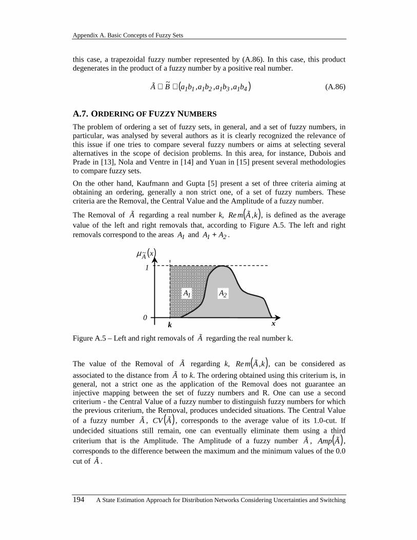
Appendix A. Basic Concepts of Fuzzy Sets
194 A State Estimation Approach for Distribution Networks Considering Uncertainties and Switching
this case, a trapezoidal fuzzy number represented by (A.86). In this case, this product degenerates in the product of a fuzzy number by a positive real number.
( )41312111 ba,ba,ba,baB~
à ≅⊗ (A.86)
A.7. ORDERING OF FUZZY NUMBERS The problem of ordering a set of fuzzy sets, in general, and a set of fuzzy numbers, in particular, was analysed by several authors as it is clearly recognized the relevance of this issue if one tries to compare several fuzzy numbers or aims at selecting several alternatives in the scope of decision problems. In this area, for instance, Dubois and Prade in [13], Nola and Ventre in [14] and Yuan in [15] present several methodologies to compare fuzzy sets.
On the other hand, Kaufmann and Gupta [5] present a set of three criteria aiming at obtaining an ordering, generally a non strict one, of a set of fuzzy numbers. These criteria are the Removal, the Central Value and the Amplitude of a fuzzy number.
The Removal of à regarding a real number k, ( )k,ÃmRe , is defined as the average value of the left and right removals that, according to Figure A.5. The left and right removals correspond to the areas 1A and 21 AA + .
0
1
x
( )xA~µ
k
2A1A
Figure A.5 – Left and right removals of à regarding the real number k.
The value of the Removal of à regarding k, ( )k,ÃmRe , can be considered as
associated to the distance from à to k. The ordering obtained using this criterium is, in general, not a strict one as the application of the Removal does not guarantee an injective mapping between the set of fuzzy numbers and R. One can use a second criterium - the Central Value of a fuzzy number to distinguish fuzzy numbers for which the previous criterium, the Removal, produces undecided situations. The Central Value of a fuzzy number à , ( )ÃCV , corresponds to the average value of its 1.0-cut. If undecided situations still remain, one can eventually eliminate them using a third criterium that is the Amplitude. The Amplitude of a fuzzy number à , ( )ÃAmp , corresponds to the difference between the maximum and the minimum values of the 0.0 cut of à .

A.8. Appendix References
A State Estimation Approach for Distribution Networks Considering Uncertainties and Switching 195
Regarding a trapezoidal fuzzy number à given by ( )4321 a,a,a,a , the Removal of Ã
regarding k=0.0 is given by (A.87). The Central Value and the Amplitude of à are given by (A.88) and (A.89).
( )4
aaaa0.0,ÃmRe 4321 +++
= (A.87)
( )2
aaÃCV 32 +
= (A.88)
( ) 14 aaÃAmp −= (A.89)
As it was already referred the successive application of these three criteria does not guarantee that a strict ordering of a set of fuzzy numbers is obtained. However, for real life applications the use of these three criteria lead, in general, to satisfactory results.
This Appendix is included in this Thesis with the purpose of highlighting several concepts that are referred along the main text. The interested reader can obtain a more detailed text in reference [16], as well as the previous references of this Appendix. The reference [16] includes more information on issues as fuzzy relations and fuzzy inference systems.
A.8. APPENDIX REFERENCES
[1] J. T. Saraiva, “Fuzzy Sets - Concepts, Definitions and Basic Operations Rules”, FEUP and INESC, Jan. 1996.
[2] L. A. Zadeh, “Fuzzy Sets”, Information and Control, Vol.º8, pp. 338-353, Aug. 1965.
[3] J. C. Bezdeck, Pattern Recognition with Fuzzy Objective Function Algorithms, Plenum Press, New York, 1981.
[4] D. Dubois, H. Prade, Théorie des Possibilités - Applications à la Representation des Connaissances en Informatique, (2e Édition), Masson, Paris, 1987.
[5] A. Kaufmann, M. M. Gupta, Fuzzy Mathematical Models in Engineering and Management Science, North Holland ed., Amsterdam, 1988.
[6] J. Llena, “On Fuzzy Linear Programming”, European Journal of Operational Research, Vol. 22, 1985.
[7] H.-J., Zimmermann, Fuzzy Set Theory and Its Applications, Kluwer, Nijhoff Publishing, Dordrecht, 1985.
[8] M. E. El-Hawary, “Fuzzy Systems: An Engineering Point of View”, Electric Power Applications of Fuzzy Systems, M. E. El-Hawary (ed), IEEE Press, Piscataway, 1998.

Appendix A. Basic Concepts of Fuzzy Sets
196 A State Estimation Approach for Distribution Networks Considering Uncertainties and Switching
[9] U. Thöle, H.-J. Zimmermann, P. Zysno, “On the Suitability of Minimum and Product Operators for the Intersection of Fuzzy Sets”, Fuzzy Sets and Systems, Vol. 2, 1979.
[10] I. B. Turksen, “Measurement of Membership Functions and their Acquisition”, Fuzzy Sets and Systems, Vol. 40, 1991.
[11] H.-J., Zimmermann, Fuzzy Set, Decision Making and Expert Systems, Kluwer Academic Publishers, Boston, 1987.
[12] D. Dubois, H. Prade, “Fuzzy Real Algebra: Some Results”, Fuzzy Sets and Systems, Vol. 2, pp. 327-348, 1979.
[13] D. Dubois, H. Prade, “The Use of Fuzzy Numbers in Decision Analysis”, Fuzzy Information and Decision Processes, M. Gupta and E. Sanchez (eds), North Holland, Amsterdam, 1982.
[14] A. Nola, A. Ventre, “Ordering via Fuzzy Entropy”, Fuzzy Information and Decision Processes, M. Gupta and E. Sanchez (eds), North Holland, Amsterdam, 1982.
[15] Y. Yuan, “Criteria for Evaluating Fuzzy Ranking Methods”, Fuzzy Sets and Systems, Vol. 44, 1991.
[16] René Jager, Fuzzy Logic in Control, PhD. Thesis, Technische Universiteit Delft, The Netherlands, ISBN90-9008318-9, 1995.

A State Estimation Approach for Distribution Networks Considering Uncertainties and Switching 197
B. DATA OF ILLUSTRATIVE NETWORKS In this Appendix will present the network used for illustrative purposes in Chapter 7. This network is based on the IEEE 24 bus Test System. For that reason, previously it will be presented this network and afterwards they will be detailed the modifications as used in Chapter 7.
B.1. IEEE 24 BUS TEST SYSTEM
B.1.1. NETWORK CHARACTERISTICS
The IEEE 24 bus Test System is represented in Figure B.1. For this network they will be presented all the characteristics needed to run a power flow exercise. These characteristics are the voltage level in each bus and the type of bus based on the equipments connected to it. These values are indicated in the second and in the third column of Table B.1. In this table they are also included the active power generation (Pg) in MW specified for each bus, the active power consumption (Pc) in MW, the reactive power generation (Qg) in Mvar, the reactive power consumption (Qc) in Mvar and the specified voltage magnitude (Vsp) in p.u..
19
17 18~
21~
22 ~
16 ~20
23 ~
1514
24 11 12
13~
3 9 10
4
12 5
7
~
8
6
138 kV230 kV
~ Sync.Cond.
~~
~
Figure B.1 – IEEE 24 bus Test System.
The buses can be of type PQ, PV or RC. The type PQ means that the active and reactive injections are known or specified. The type PV means that the bus has a generation

Appendix B. Data of Illustrative Networks
198 A State Estimation Approach for Distribution Networks Considering Uncertainties and Switching
capability by a generator or by a connection to another network. For these buses they must be known or specified the values for the active injected power and the voltage magnitude. The RC bus is selected among the buses of type PV and, in general, is the bus of the island with type PV that has the largest generation capability. In each energised island of the network there is a bus of this type. For the buses of type RC it must be known or specified the voltage magnitude. This bus is also the reference for the voltage phases, which means that a value for the voltage phase must be specified and the voltage phases in the other buses are evaluated using this value as reference.
Bus# type Vn
(kV) Pg
(MW) Pc
(MW) Qg
(Mvar) Qc
(Mvar) Vsp. (pu)
1 RC 138 0 108 0 22 1.075 2 PV 138 167 97 0 20 1.075 3 PQ 138 0 180 0 37 - 4 PQ 138 0 74 0 15 - 5 PQ 138 0 71 0 14 - 6 PQ 138 0 136 0 28 - 7 PV 138 250 125 0 25 1.075 8 PQ 138 0 171 0 35 - 9 PQ 138 0 175 0 36 -
10 PQ 138 0 195 0 40 - 11 PQ 230 0 0 0 0 - 12 PQ 230 0 0 0 0 - 13 PV 230 541 265 0 54 1.025 14 PQ 230 0 194 0 39 - 15 PV 230 190 317 0 64 1.025 16 PV 230 130 100 0 20 1.025 17 PQ 230 0 0 0 0 - 18 PV 230 350 333 0 68 1.025 19 PQ 230 0 181 0 37 - 20 PQ 230 0 128 0 26 - 21 PV 230 350 0 0 0 1.025 22 PV 230 250 0 0 0 1.025 23 PV 230 505 0 0 0 1.025 24 PQ 230 0 0 0 0 -
Table B.1 – Characteristics of the buses of the IEEE 24 bus Test System.
For this network they are presented in Table B.2 all branch characteristics needed to run a power flow algorithm. These characteristics are the branch resistance (R) in p.u., the branch reactance (X) in p.u. and the branch shunt susceptance (Ysh) in 1000×p.u.. These per unit (p.u.) values are obtained by using as power base the value of 500 MVA and as voltage base in this case was used the nominal voltage on each bus.
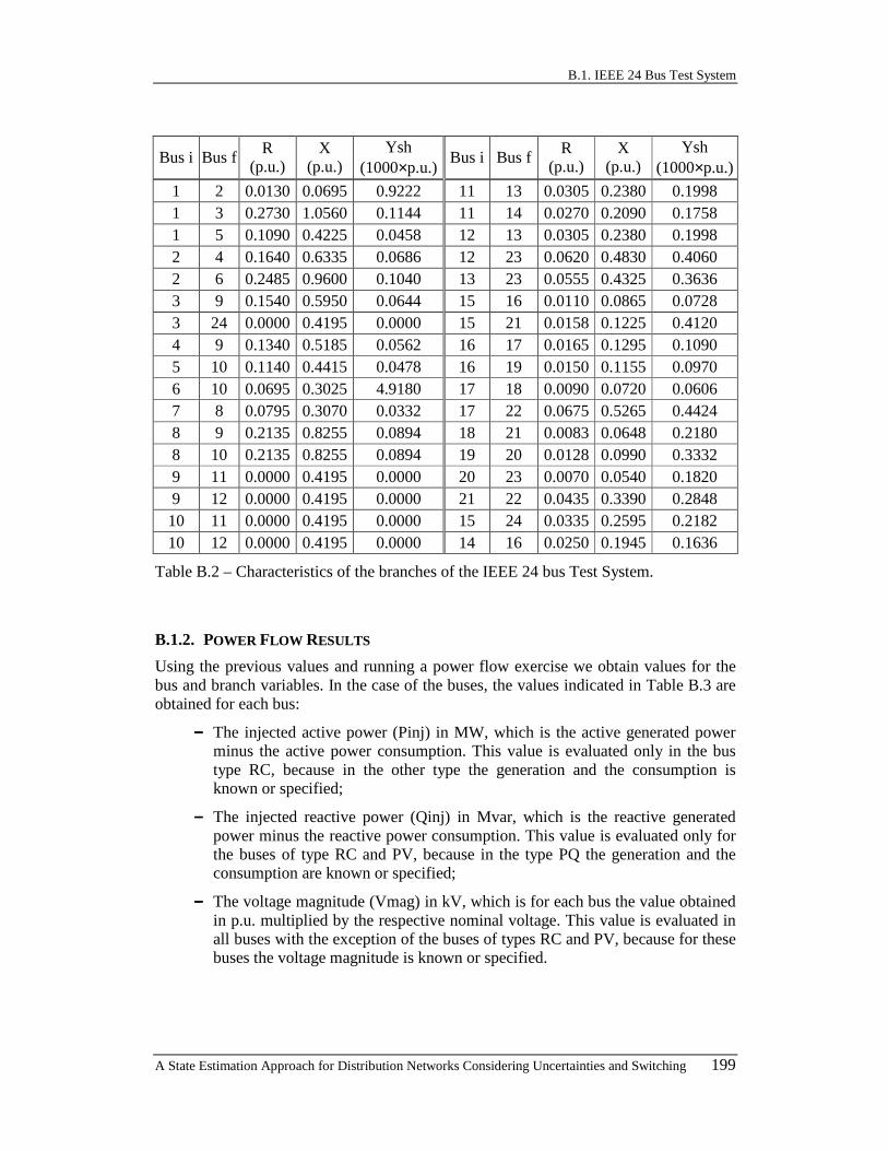
B.1. IEEE 24 Bus Test System
A State Estimation Approach for Distribution Networks Considering Uncertainties and Switching 199
Bus i Bus f R
(p.u.) X
(p.u.) Ysh
(1000×p.u.) Bus i Bus f
R (p.u.)
X (p.u.)
Ysh (1000×p.u.)
1 2 0.0130 0.0695 0.9222 11 13 0.0305 0.2380 0.1998 1 3 0.2730 1.0560 0.1144 11 14 0.0270 0.2090 0.1758 1 5 0.1090 0.4225 0.0458 12 13 0.0305 0.2380 0.1998 2 4 0.1640 0.6335 0.0686 12 23 0.0620 0.4830 0.4060 2 6 0.2485 0.9600 0.1040 13 23 0.0555 0.4325 0.3636 3 9 0.1540 0.5950 0.0644 15 16 0.0110 0.0865 0.0728 3 24 0.0000 0.4195 0.0000 15 21 0.0158 0.1225 0.4120 4 9 0.1340 0.5185 0.0562 16 17 0.0165 0.1295 0.1090 5 10 0.1140 0.4415 0.0478 16 19 0.0150 0.1155 0.0970 6 10 0.0695 0.3025 4.9180 17 18 0.0090 0.0720 0.0606 7 8 0.0795 0.3070 0.0332 17 22 0.0675 0.5265 0.4424 8 9 0.2135 0.8255 0.0894 18 21 0.0083 0.0648 0.2180 8 10 0.2135 0.8255 0.0894 19 20 0.0128 0.0990 0.3332 9 11 0.0000 0.4195 0.0000 20 23 0.0070 0.0540 0.1820 9 12 0.0000 0.4195 0.0000 21 22 0.0435 0.3390 0.2848 10 11 0.0000 0.4195 0.0000 15 24 0.0335 0.2595 0.2182 10 12 0.0000 0.4195 0.0000 14 16 0.0250 0.1945 0.1636
Table B.2 – Characteristics of the branches of the IEEE 24 bus Test System.
B.1.2. POWER FLOW RESULTS
Using the previous values and running a power flow exercise we obtain values for the bus and branch variables. In the case of the buses, the values indicated in Table B.3 are obtained for each bus:
−−−− The injected active power (Pinj) in MW, which is the active generated power minus the active power consumption. This value is evaluated only in the bus type RC, because in the other type the generation and the consumption is known or specified;
−−−− The injected reactive power (Qinj) in Mvar, which is the reactive generated power minus the reactive power consumption. This value is evaluated only for the buses of type RC and PV, because in the type PQ the generation and the consumption are known or specified;
−−−− The voltage magnitude (Vmag) in kV, which is for each bus the value obtained in p.u. multiplied by the respective nominal voltage. This value is evaluated in all buses with the exception of the buses of types RC and PV, because for these buses the voltage magnitude is known or specified.
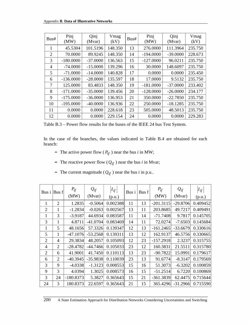
Appendix B. Data of Illustrative Networks
200 A State Estimation Approach for Distribution Networks Considering Uncertainties and Switching
Bus# Pinj
(MW) Qinj
(Mvar) Vmag (kV)
Bus# Pinj
(MW) Qinj
(Mvar) Vmag (kV)
1 45.5304 101.5196 148.350 13 276.0000 111.3964 235.750 2 70.0000 89.9245 148.350 14 -194.0000 -39.0000 228.673 3 -180.0000 -37.0000 136.563 15 -127.0000 96.0211 235.750 4 -74.0000 -15.0000 139.296 16 30.0000 148.6097 235.750 5 -71.0000 -14.0000 140.828 17 0.0000 0.0000 235.450 6 -136.0000 -28.0000 135.597 18 17.0000 9.5132 235.750 7 125.0000 83.4833 148.350 19 -181.0000 -37.0000 233.402 8 -171.0000 -35.0000 139.456 20 -128.0000 -26.0000 234.177 9 -175.0000 -36.0000 136.953 21 350.0000 -22.7850 235.750 10 -195.0000 -40.0000 136.936 22 250.0000 -18.1285 235.750 11 0.0000 0.0000 228.618 23 505.0000 48.5013 235.750 12 0.0000 0.0000 229.154 24 0.0000 0.0000 229.283
Table B.3 – Power flow results for the buses of the IEEE 24 bus Test System.
In the case of the branches, the values indicated in Table B.4 are obtained for each branch:
−−−− The active power flow ( ifP ) near the bus i in MW;
−−−− The reactive power flow ( ifQ ) near the bus i in Mvar;
−−−− The current magnitude ( ifQ ) near the bus i in p.u..
Bus i Bus f ifP
(MW) ifQ
(Mvar) ifI
(p.u.) Bus i Bus f ifP
(MW) ifQ
(Mvar) ifI
(p.u.)
1 2 1.2835 -0.5064 0.002388 11 13 -201.3115 -29.8706 0.409452 2 1 -1.2834 -0.0263 0.002567 13 11 203.8685 49.7217 0.409491 1 3 -3.9187 44.6934 0.083587 11 14 -71.7408 9.7817 0.145705 3 1 4.8711 -41.0704 0.083469 14 11 72.0274 -7.6503 0.145684 1 5 48.1656 57.3326 0.139347 12 13 -161.2465 -33.6679 0.330616 5 1 -47.1076 -53.2568 0.139311 13 12 162.9137 46.5756 0.330665 2 4 29.3834 48.2057 0.105093 12 23 -157.2918 2.3237 0.315755 4 2 -28.4782 -44.7466 0.105033 23 12 160.3831 21.5511 0.315780 2 6 41.9001 41.7450 0.110113 13 23 -90.7822 15.0991 0.179617 6 2 -40.3945 -35.9838 0.110039 23 13 91.6774 -8.3147 0.179569 3 9 -4.0338 -1.3123 0.008553 15 16 51.3073 -6.3202 0.100859 9 3 4.0394 1.3025 0.008573 16 15 -51.2514 6.7220 0.100869 3 24 -180.8373 5.3827 0.365643 15 21 -361.3839 62.4475 0.715644
24 3 180.8373 22.6597 0.365643 21 15 365.4296 -31.2966 0.715590

B.2. Augmented Network Based on the IEEE 24 Test System
A State Estimation Approach for Distribution Networks Considering Uncertainties and Switching 201
Bus i Bus f ifP
(MW) ifQ
(Mvar) ifI
(p.u.) Bus i Bus f ifP
(MW) ifQ
(Mvar) ifI
(p.u.)
4 9 -45.5218 29.7466 0.107776 16 17 -245.8510 44.2764 0.487443 9 4 46.2998 -26.7642 0.107746 17 16 247.8111 -28.9494 0.487427 5 10 -23.8924 39.2568 0.090107 16 19 57.4457 38.1092 0.134566
10 5 24.3550 -37.4895 0.090066 19 16 -57.3100 -37.1143 0.134511 6 10 -95.6055 7.9838 0.195593 17 18 -131.9732 8.4141 0.258364
10 6 96.9336 -4.6011 0.195277 18 17 132.2736 -6.0429 0.258361 7 8 125.0000 83.4833 0.279673 17 22 -115.8379 20.5352 0.229895 8 7 -121.8911 -71.4958 0.279655 22 17 117.6214 -6.8557 0.229842 8 9 -33.3388 20.9404 0.077963 18 21 -115.2736 15.5560 0.226991 9 8 33.9873 -18.4778 0.077917 21 18 115.4874 -14.0013 0.226963 8 10 -15.7701 15.5554 0.043901 19 20 -123.6900 0.1143 0.243770
10 8 15.9756 -14.8058 0.043840 20 19 124.0704 2.6551 0.243774 9 11 -118.2902 4.0942 0.238532 20 23 -252.0704 -28.6551 0.498314
11 9 118.2902 7.8401 0.238532 23 20 252.9395 35.2650 0.498338 9 12 -141.0363 3.8452 0.284335 21 22 -130.9170 22.5129 0.259234
12 9 141.0363 13.1123 0.284335 22 21 132.3786 -11.2728 0.259197 10 11 -154.7621 8.2173 0.312369 15 24 183.0765 39.8938 0.365643 11 10 154.7621 12.2488 0.312369 24 15 -180.8373 -22.6597 0.365605 10 12 -177.5021 8.6791 0.358190 14 16 -266.0274 -31.3497 0.538817 12 10 177.5021 18.2319 0.358190 16 14 269.6567 59.5021 0.538844
Table B.4 – Power flow results for the branches of the IEEE 24 bus Test System.
B.2. AUGMENTED NETWORK BASED ON THE IEEE 24 TEST SYSTEM
B.2.1. NETWORK CHARACTERISTICS
The second network is based on the IEEE 24 bus Test System and it is represented in Figure B.2. This network was used in Chapter 7 as an illustrative network. As for the previous network, for this network we will present all the characteristics needed to run a power flow exercise. These can be bus characteristics (Table B.5) and branch characteristics (Table B.6).
The values and the symbols that appear in Table B.5 have the same meaning as indicated for Table B.1. The buses not included in Table B.5 have the same values as indicated for the previous network, and buses 3 and 6 are included in this table because the values of the Pc and Qc are different.
The values and the symbols that appear in Table B.6 have the same meaning as indicated for Table B.2. In this case, in Table B.6 they are only included the branches that were added to this network. The branches that belong to the IEEE 24 bus Test System have the same characteristics as indicated before.

Appendix B. Data of Illustrative Networks
202 A State Estimation Approach for Distribution Networks Considering Uncertainties and Switching
19
17 18 21 22
1620
23
1514
24 11 12
13
3 9 10
4
12 5
7
8
6
138 kV230 kV
Measures:- Power- Voltage
Sync.Cond.
30 kV138 kV
39
41
43
46
47
4840
51 52
49
50
42
44
45
25
27
30
34
35
2826
36 38
31
37
29
32
33
19
17 18 21 22
1620
23
1514
24 11 12
13
3 9 10
4
12 5
7
8
6
138 kV230 kV
Measures:- Power- Voltage
Sync.Cond.
30 kV138 kV
39
41
4343
4646
4747
48484040
5151 5252
4949
50
4242
4444
4545
25
27
3030
3434
3535
28282626
3636 3838
3131
3737
2929
3232
3333
Figure B.2 – Augmented network based on the IEEE 24 bus network with a new voltage level at 30 kV.
Bus# type Vn
(kV) Pg
(MW) Pc
(MW) Qg
(Mvar) Qc
(Mvar) Vsp. (pu)
3 PQ 138 0 0 0 0 - 6 PQ 138 0 0 0 0 -
25 PQ 30 0 0 0 0 - 26 PQ 30 0 25 0 5.1 - 27 PQ 30 0 25 0 5.1 - 28 PQ 30 0 25 0 5.1 - 29 PQ 30 0 15 0 3.1 - 30 PQ 30 0 15 0 3.1 - 31 PQ 30 0 15 0 3.1 -
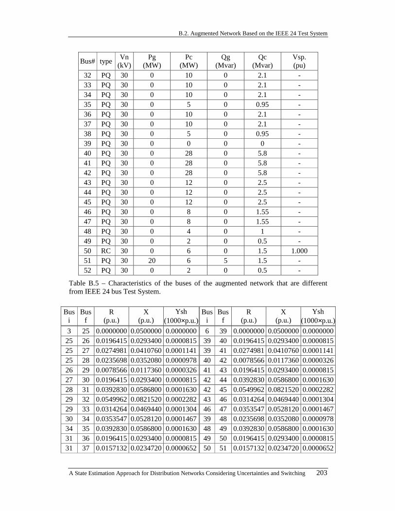
B.2. Augmented Network Based on the IEEE 24 Test System
A State Estimation Approach for Distribution Networks Considering Uncertainties and Switching 203
Bus# type Vn
(kV) Pg
(MW) Pc
(MW) Qg
(Mvar) Qc
(Mvar) Vsp. (pu)
32 PQ 30 0 10 0 2.1 - 33 PQ 30 0 10 0 2.1 - 34 PQ 30 0 10 0 2.1 - 35 PQ 30 0 5 0 0.95 - 36 PQ 30 0 10 0 2.1 - 37 PQ 30 0 10 0 2.1 - 38 PQ 30 0 5 0 0.95 - 39 PQ 30 0 0 0 0 - 40 PQ 30 0 28 0 5.8 - 41 PQ 30 0 28 0 5.8 - 42 PQ 30 0 28 0 5.8 - 43 PQ 30 0 12 0 2.5 - 44 PQ 30 0 12 0 2.5 - 45 PQ 30 0 12 0 2.5 - 46 PQ 30 0 8 0 1.55 - 47 PQ 30 0 8 0 1.55 - 48 PQ 30 0 4 0 1 - 49 PQ 30 0 2 0 0.5 - 50 RC 30 0 6 0 1.5 1.000 51 PQ 30 20 6 5 1.5 - 52 PQ 30 0 2 0 0.5 -
Table B.5 – Characteristics of the buses of the augmented network that are different from IEEE 24 bus Test System.
Bus i
Bus f
R (p.u.)
X (p.u.)
Ysh (1000×p.u.)
Bus i
Bus f
R (p.u.)
X (p.u.)
Ysh (1000×p.u.)
3 25 0.0000000 0.0500000 0.0000000 6 39 0.0000000 0.0500000 0.0000000 25 26 0.0196415 0.0293400 0.0000815 39 40 0.0196415 0.0293400 0.0000815 25 27 0.0274981 0.0410760 0.0001141 39 41 0.0274981 0.0410760 0.0001141 25 28 0.0235698 0.0352080 0.0000978 40 42 0.0078566 0.0117360 0.0000326 26 29 0.0078566 0.0117360 0.0000326 41 43 0.0196415 0.0293400 0.0000815 27 30 0.0196415 0.0293400 0.0000815 42 44 0.0392830 0.0586800 0.0001630 28 31 0.0392830 0.0586800 0.0001630 42 45 0.0549962 0.0821520 0.0002282 29 32 0.0549962 0.0821520 0.0002282 43 46 0.0314264 0.0469440 0.0001304 29 33 0.0314264 0.0469440 0.0001304 46 47 0.0353547 0.0528120 0.0001467 30 34 0.0353547 0.0528120 0.0001467 39 48 0.0235698 0.0352080 0.0000978 34 35 0.0392830 0.0586800 0.0001630 48 49 0.0392830 0.0586800 0.0001630 31 36 0.0196415 0.0293400 0.0000815 49 50 0.0196415 0.0293400 0.0000815 31 37 0.0157132 0.0234720 0.0000652 50 51 0.0157132 0.0234720 0.0000652
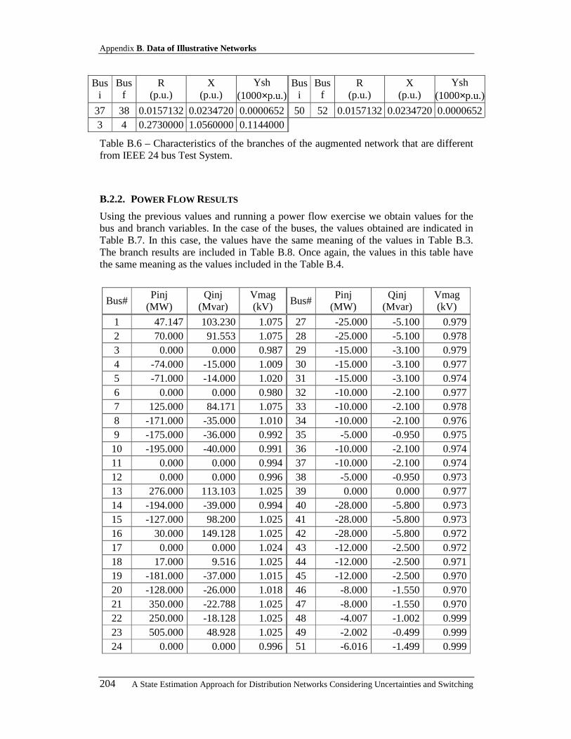
Appendix B. Data of Illustrative Networks
204 A State Estimation Approach for Distribution Networks Considering Uncertainties and Switching
Bus i
Bus f
R (p.u.)
X (p.u.)
Ysh (1000×p.u.)
Bus i
Bus f
R (p.u.)
X (p.u.)
Ysh (1000×p.u.)
37 38 0.0157132 0.0234720 0.0000652 50 52 0.0157132 0.0234720 0.0000652 3 4 0.2730000 1.0560000 0.1144000
Table B.6 – Characteristics of the branches of the augmented network that are different from IEEE 24 bus Test System.
B.2.2. POWER FLOW RESULTS
Using the previous values and running a power flow exercise we obtain values for the bus and branch variables. In the case of the buses, the values obtained are indicated in Table B.7. In this case, the values have the same meaning of the values in Table B.3. The branch results are included in Table B.8. Once again, the values in this table have the same meaning as the values included in the Table B.4.
Bus# Pinj
(MW) Qinj
(Mvar) Vmag (kV)
Bus# Pinj
(MW) Qinj
(Mvar) Vmag (kV)
1 47.147 103.230 1.075 27 -25.000 -5.100 0.979 2 70.000 91.553 1.075 28 -25.000 -5.100 0.978 3 0.000 0.000 0.987 29 -15.000 -3.100 0.979 4 -74.000 -15.000 1.009 30 -15.000 -3.100 0.977 5 -71.000 -14.000 1.020 31 -15.000 -3.100 0.974 6 0.000 0.000 0.980 32 -10.000 -2.100 0.977 7 125.000 84.171 1.075 33 -10.000 -2.100 0.978 8 -171.000 -35.000 1.010 34 -10.000 -2.100 0.976 9 -175.000 -36.000 0.992 35 -5.000 -0.950 0.975 10 -195.000 -40.000 0.991 36 -10.000 -2.100 0.974 11 0.000 0.000 0.994 37 -10.000 -2.100 0.974 12 0.000 0.000 0.996 38 -5.000 -0.950 0.973 13 276.000 113.103 1.025 39 0.000 0.000 0.977 14 -194.000 -39.000 0.994 40 -28.000 -5.800 0.973 15 -127.000 98.200 1.025 41 -28.000 -5.800 0.973 16 30.000 149.128 1.025 42 -28.000 -5.800 0.972 17 0.000 0.000 1.024 43 -12.000 -2.500 0.972 18 17.000 9.516 1.025 44 -12.000 -2.500 0.971 19 -181.000 -37.000 1.015 45 -12.000 -2.500 0.970 20 -128.000 -26.000 1.018 46 -8.000 -1.550 0.970 21 350.000 -22.788 1.025 47 -8.000 -1.550 0.970 22 250.000 -18.128 1.025 48 -4.007 -1.002 0.999 23 505.000 48.928 1.025 49 -2.002 -0.499 0.999 24 0.000 0.000 0.996 51 -6.016 -1.499 0.999
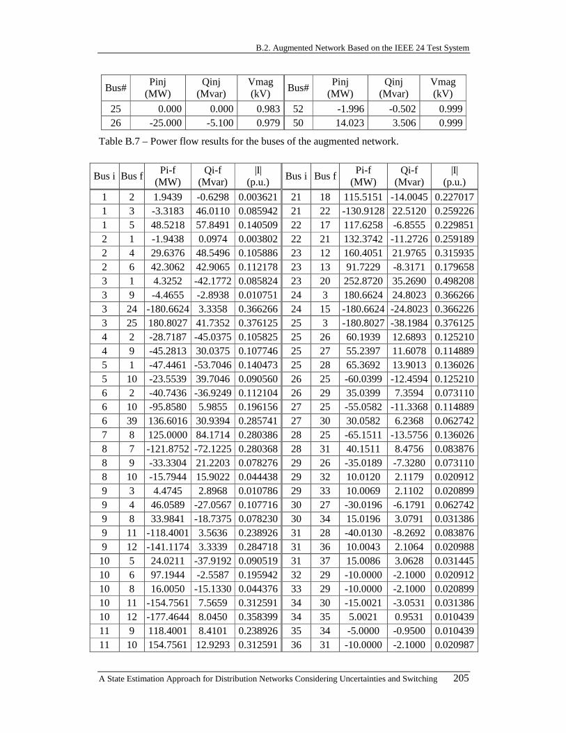
B.2. Augmented Network Based on the IEEE 24 Test System
A State Estimation Approach for Distribution Networks Considering Uncertainties and Switching 205
Bus# Pinj
(MW) Qinj
(Mvar) Vmag (kV)
Bus# Pinj
(MW) Qinj
(Mvar) Vmag (kV)
25 0.000 0.000 0.983 52 -1.996 -0.502 0.999 26 -25.000 -5.100 0.979 50 14.023 3.506 0.999
Table B.7 – Power flow results for the buses of the augmented network.
Bus i Bus f Pi-f
(MW) Qi-f
(Mvar) |I|
(p.u.) Bus i Bus f
Pi-f (MW)
Qi-f (Mvar)
|I| (p.u.)
1 2 1.9439 -0.6298 0.003621 21 18 115.5151 -14.0045 0.227017 1 3 -3.3183 46.0110 0.085942 21 22 -130.9128 22.5120 0.259226 1 5 48.5218 57.8491 0.140509 22 17 117.6258 -6.8555 0.229851 2 1 -1.9438 0.0974 0.003802 22 21 132.3742 -11.2726 0.259189 2 4 29.6376 48.5496 0.105886 23 12 160.4051 21.9765 0.315935 2 6 42.3062 42.9065 0.112178 23 13 91.7229 -8.3171 0.179658 3 1 4.3252 -42.1772 0.085824 23 20 252.8720 35.2690 0.498208 3 9 -4.4655 -2.8938 0.010751 24 3 180.6624 24.8023 0.366266 3 24 -180.6624 3.3358 0.366266 24 15 -180.6624 -24.8023 0.366226 3 25 180.8027 41.7352 0.376125 25 3 -180.8027 -38.1984 0.376125 4 2 -28.7187 -45.0375 0.105825 25 26 60.1939 12.6893 0.125210 4 9 -45.2813 30.0375 0.107746 25 27 55.2397 11.6078 0.114889 5 1 -47.4461 -53.7046 0.140473 25 28 65.3692 13.9013 0.136026 5 10 -23.5539 39.7046 0.090560 26 25 -60.0399 -12.4594 0.125210 6 2 -40.7436 -36.9249 0.112104 26 29 35.0399 7.3594 0.073110 6 10 -95.8580 5.9855 0.196156 27 25 -55.0582 -11.3368 0.114889 6 39 136.6016 30.9394 0.285741 27 30 30.0582 6.2368 0.062742 7 8 125.0000 84.1714 0.280386 28 25 -65.1511 -13.5756 0.136026 8 7 -121.8752 -72.1225 0.280368 28 31 40.1511 8.4756 0.083876 8 9 -33.3304 21.2203 0.078276 29 26 -35.0189 -7.3280 0.073110 8 10 -15.7944 15.9022 0.044438 29 32 10.0120 2.1179 0.020912 9 3 4.4745 2.8968 0.010786 29 33 10.0069 2.1102 0.020899 9 4 46.0589 -27.0567 0.107716 30 27 -30.0196 -6.1791 0.062742 9 8 33.9841 -18.7375 0.078230 30 34 15.0196 3.0791 0.031386 9 11 -118.4001 3.5636 0.238926 31 28 -40.0130 -8.2692 0.083876 9 12 -141.1174 3.3339 0.284718 31 36 10.0043 2.1064 0.020988
10 5 24.0211 -37.9192 0.090519 31 37 15.0086 3.0628 0.031445 10 6 97.1944 -2.5587 0.195942 32 29 -10.0000 -2.1000 0.020912 10 8 16.0050 -15.1330 0.044376 33 29 -10.0000 -2.1000 0.020899 10 11 -154.7561 7.5659 0.312591 34 30 -15.0021 -3.0531 0.031386 10 12 -177.4644 8.0450 0.358399 34 35 5.0021 0.9531 0.010439 11 9 118.4001 8.4101 0.238926 35 34 -5.0000 -0.9500 0.010439 11 10 154.7561 12.9293 0.312591 36 31 -10.0000 -2.1000 0.020987
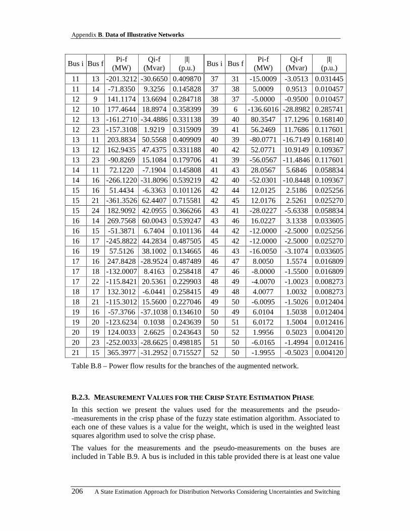
Appendix B. Data of Illustrative Networks
206 A State Estimation Approach for Distribution Networks Considering Uncertainties and Switching
Bus i Bus f Pi-f
(MW) Qi-f
(Mvar) |I|
(p.u.) Bus i Bus f
Pi-f (MW)
Qi-f (Mvar)
|I| (p.u.)
11 13 -201.3212 -30.6650 0.409870 37 31 -15.0009 -3.0513 0.031445 11 14 -71.8350 9.3256 0.145828 37 38 5.0009 0.9513 0.010457 12 9 141.1174 13.6694 0.284718 38 37 -5.0000 -0.9500 0.010457 12 10 177.4644 18.8974 0.358399 39 6 -136.6016 -28.8982 0.285741 12 13 -161.2710 -34.4886 0.331138 39 40 80.3547 17.1296 0.168140 12 23 -157.3108 1.9219 0.315909 39 41 56.2469 11.7686 0.117601 13 11 203.8834 50.5568 0.409909 40 39 -80.0771 -16.7149 0.168140 13 12 162.9435 47.4375 0.331188 40 42 52.0771 10.9149 0.109367 13 23 -90.8269 15.1084 0.179706 41 39 -56.0567 -11.4846 0.117601 14 11 72.1220 -7.1904 0.145808 41 43 28.0567 5.6846 0.058834 14 16 -266.1220 -31.8096 0.539219 42 40 -52.0301 -10.8448 0.109367 15 16 51.4434 -6.3363 0.101126 42 44 12.0125 2.5186 0.025256 15 21 -361.3526 62.4407 0.715581 42 45 12.0176 2.5261 0.025270 15 24 182.9092 42.0955 0.366266 43 41 -28.0227 -5.6338 0.058834 16 14 269.7568 60.0043 0.539247 43 46 16.0227 3.1338 0.033605 16 15 -51.3871 6.7404 0.101136 44 42 -12.0000 -2.5000 0.025256 16 17 -245.8822 44.2834 0.487505 45 42 -12.0000 -2.5000 0.025270 16 19 57.5126 38.1002 0.134665 46 43 -16.0050 -3.1074 0.033605 17 16 247.8428 -28.9524 0.487489 46 47 8.0050 1.5574 0.016809 17 18 -132.0007 8.4163 0.258418 47 46 -8.0000 -1.5500 0.016809 17 22 -115.8421 20.5361 0.229903 48 49 -4.0070 -1.0023 0.008273 18 17 132.3012 -6.0441 0.258415 49 48 4.0077 1.0032 0.008273 18 21 -115.3012 15.5600 0.227046 49 50 -6.0095 -1.5026 0.012404 19 16 -57.3766 -37.1038 0.134610 50 49 6.0104 1.5038 0.012404 19 20 -123.6234 0.1038 0.243639 50 51 6.0172 1.5004 0.012416 20 19 124.0033 2.6625 0.243643 50 52 1.9956 0.5023 0.004120 20 23 -252.0033 -28.6625 0.498185 51 50 -6.0165 -1.4994 0.012416 21 15 365.3977 -31.2952 0.715527 52 50 -1.9955 -0.5023 0.004120
Table B.8 – Power flow results for the branches of the augmented network.
B.2.3. MEASUREMENT VALUES FOR THE CRISP STATE ESTIMATION PHASE
In this section we present the values used for the measurements and the pseudo--measurements in the crisp phase of the fuzzy state estimation algorithm. Associated to each one of these values is a value for the weight, which is used in the weighted least squares algorithm used to solve the crisp phase.
The values for the measurements and the pseudo-measurements on the buses are included in Table B.9. A bus is included in this table provided there is at least one value

B.2. Augmented Network Based on the IEEE 24 Test System
A State Estimation Approach for Distribution Networks Considering Uncertainties and Switching 207
available. One bus can have four different measurement values that are indicated in the following paragraphs:
−−−− The injected active power (Pinj) in MW;
−−−− The injected reactive power (Qinj) in Mvar;
−−−− The voltage magnitude (Vmag) in p.u.;
−−−− The voltage phase (Vphase) in radians.
The values for the measurements and the pseudo-measurements on the branches are included in Table B.10. A branch is included in this table provided there is at least a value available. The active power flow is represented in this table by the symbol ifP
and the values are in MW. On the other hand, the reactive power flow is represented in this table by the symbol ifQ and the values are in Mvar.
Pinj Qinj Vmag Vphase Bus
# MW weight Mvar weight p.u. weight rad weight
1 - - - - 1.0750 100 0 1000000 2 70.0000 100 91.5535 100 1.0750 100 0 0.000001 3 0.0000 100 0.0000 100 0.9867 100 - - 5 -71.0000 100 -14.0000 100 - - - - 6 0.0000 100 0.0000 100 0.9803 100 - - 7 125.0000 100 84.1714 100 1.0750 100 0 0.000001 8 -171.0000 100 -35.0000 100 - - - - 9 -175.0000 100 -36.0000 100 - - - - 10 -195.0000 100 -40.0000 100 - - - - 11 0.0000 100 0.0000 100 0.9936 1 - - 12 0.0000 100 0.0000 100 0.9959 1 - - 13 276.0000 100 113.1027 100 1.0250 100 0 0.000001 14 -194.0000 1 -39.0000 1 0.9940 1 - - 15 -127.0000 100 98.1999 100 1.0250 100 0 0.000001 16 30.0000 100 149.1282 100 1.0250 100 0 0.000001 17 0.0000 100 0.0000 100 - - - - 18 - - - - 1.0250 1 0 0.000001 21 350.0000 1 -23.0000 1 1.0250 1 0 0.000001 22 250.0000 1 -18.0000 1 1.0250 1 0 0.000001 23 505.0000 100 48.9284 100 1.0250 100 0 0.000001 24 0.0000 1 0.0000 1 0.9958 1 - - 25 0.0000 100 0.0000 100 - - - - 26 -26.38 0.1 -5.56 0.1 - - - - 27 -25.85 0.1 -5.66 0.1 - - - - 28 -27.30 0.1 -5.86 0.1 - - - - 29 -14.35 0.1 -2.93 0.1 - - - -
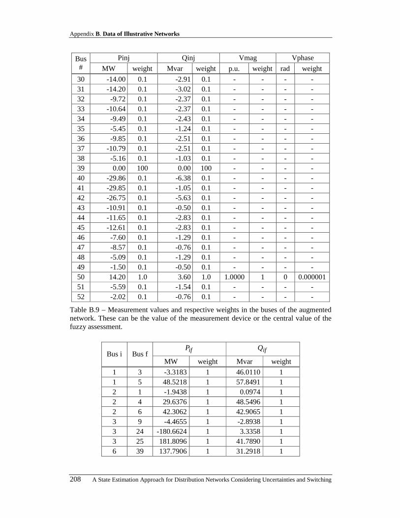
Appendix B. Data of Illustrative Networks
208 A State Estimation Approach for Distribution Networks Considering Uncertainties and Switching
Pinj Qinj Vmag Vphase Bus# MW weight Mvar weight p.u. weight rad weight
30 -14.00 0.1 -2.91 0.1 - - - - 31 -14.20 0.1 -3.02 0.1 - - - - 32 -9.72 0.1 -2.37 0.1 - - - - 33 -10.64 0.1 -2.37 0.1 - - - - 34 -9.49 0.1 -2.43 0.1 - - - - 35 -5.45 0.1 -1.24 0.1 - - - - 36 -9.85 0.1 -2.51 0.1 - - - - 37 -10.79 0.1 -2.51 0.1 - - - - 38 -5.16 0.1 -1.03 0.1 - - - - 39 0.00 100 0.00 100 - - - - 40 -29.86 0.1 -6.38 0.1 - - - - 41 -29.85 0.1 -1.05 0.1 - - - - 42 -26.75 0.1 -5.63 0.1 - - - - 43 -10.91 0.1 -0.50 0.1 - - - - 44 -11.65 0.1 -2.83 0.1 - - - - 45 -12.61 0.1 -2.83 0.1 - - - - 46 -7.60 0.1 -1.29 0.1 - - - - 47 -8.57 0.1 -0.76 0.1 - - - - 48 -5.09 0.1 -1.29 0.1 - - - - 49 -1.50 0.1 -0.50 0.1 - - - - 50 14.20 1.0 3.60 1.0 1.0000 1 0 0.000001 51 -5.59 0.1 -1.54 0.1 - - - - 52 -2.02 0.1 -0.76 0.1 - - - -
Table B.9 – Measurement values and respective weights in the buses of the augmented network. These can be the value of the measurement device or the central value of the fuzzy assessment.
ifP ifQ Bus i Bus f
MW weight Mvar weight
1 3 -3.3183 1 46.0110 1 1 5 48.5218 1 57.8491 1 2 1 -1.9438 1 0.0974 1 2 4 29.6376 1 48.5496 1 2 6 42.3062 1 42.9065 1 3 9 -4.4655 1 -2.8938 1 3 24 -180.6624 1 3.3358 1 3 25 181.8096 1 41.7890 1 6 39 137.7906 1 31.2918 1
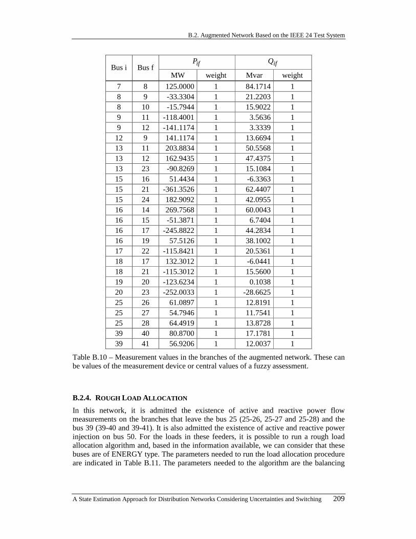
B.2. Augmented Network Based on the IEEE 24 Test System
A State Estimation Approach for Distribution Networks Considering Uncertainties and Switching 209
ifP ifQ Bus i Bus f
MW weight Mvar weight
7 8 125.0000 1 84.1714 1 8 9 -33.3304 1 21.2203 1 8 10 -15.7944 1 15.9022 1 9 11 -118.4001 1 3.5636 1 9 12 -141.1174 1 3.3339 1
12 9 141.1174 1 13.6694 1 13 11 203.8834 1 50.5568 1 13 12 162.9435 1 47.4375 1 13 23 -90.8269 1 15.1084 1 15 16 51.4434 1 -6.3363 1 15 21 -361.3526 1 62.4407 1 15 24 182.9092 1 42.0955 1 16 14 269.7568 1 60.0043 1 16 15 -51.3871 1 6.7404 1 16 17 -245.8822 1 44.2834 1 16 19 57.5126 1 38.1002 1 17 22 -115.8421 1 20.5361 1 18 17 132.3012 1 -6.0441 1 18 21 -115.3012 1 15.5600 1 19 20 -123.6234 1 0.1038 1 20 23 -252.0033 1 -28.6625 1 25 26 61.0897 1 12.8191 1 25 27 54.7946 1 11.7541 1 25 28 64.4919 1 13.8728 1 39 40 80.8700 1 17.1781 1 39 41 56.9206 1 12.0037 1
Table B.10 – Measurement values in the branches of the augmented network. These can be values of the measurement device or central values of a fuzzy assessment.
B.2.4. ROUGH LOAD ALLOCATION
In this network, it is admitted the existence of active and reactive power flow measurements on the branches that leave the bus 25 (25-26, 25-27 and 25-28) and the bus 39 (39-40 and 39-41). It is also admitted the existence of active and reactive power injection on bus 50. For the loads in these feeders, it is possible to run a rough load allocation algorithm and, based in the information available, we can consider that these buses are of ENERGY type. The parameters needed to run the load allocation procedure are indicated in Table B.11. The parameters needed to the algorithm are the balancing

Appendix B. Data of Illustrative Networks
210 A State Estimation Approach for Distribution Networks Considering Uncertainties and Switching
parameter m (we considered a value of 0.5); uncertainty parameter x (we used the value 5%); and balancing parameter λ (we used the value 0.5).
Bus# peakP
(MW) installedP (MW)
aveP (MW)
peakQ
(Mvar) installedQ (Mvar)
aveQ (Mvar)
26 50.00 75.00 28.25 12.75 20.40 6.67 27 50.00 75.00 27.00 10.20 16.30 5.60 28 50.00 80.00 27.00 10.20 16.30 5.60 29 30.00 45.00 13.75 7.75 10.90 3.25 30 30.00 45.00 13.00 6.20 8.70 2.60 31 30.00 42.00 13.00 6.20 8.70 2.60 32 20.00 30.00 9.50 5.25 7.90 3.04 33 20.00 30.00 11.50 5.25 7.90 3.04 34 20.00 30.00 9.00 4.20 6.30 2.60 35 10.00 15.00 6.00 1.90 2.90 1.45 36 20.00 30.00 9.00 4.20 6.30 2.60 37 20.00 30.00 11.00 4.20 6.30 2.60 38 10.00 15.00 5.00 1.90 2.90 0.95 40 56.00 89.60 30.00 11.60 18.60 6.30 41 56.00 89.60 30.00 2.00 3.20 1.00 42 56.00 78.40 26.00 11.60 16.20 5.30 43 24.00 33.60 10.00 1.00 1.40 0.50 44 24.00 36.00 11.00 5.00 7.50 3.00 45 24.00 36.00 13.00 5.00 7.50 3.00 46 16.00 24.00 7.00 3.00 4.50 1.00 47 16.00 24.00 9.00 1.00 1.50 1.00 48 8.00 12.80 6.00 2.00 3.20 1.50 49 4.00 5.60 1.00 1.00 1.40 0.50 51 12.00 18.00 5.00 3.00 4.50 1.50 52 4.00 6.00 2.00 1.00 1.50 1.00
Table B.11 – Values for the parameters used to run the fuzzy load allocation algorithm for all the loads on the feeders included in the IEEE 24 bus network.
After running the referred algorithm in each sub-network they are obtained the sets of values ( )maxallocmin P ;P ;P and ( )maxallocmin Q ;Q ;Q that will be used as input of the
Fuzzy State Estimation algorithm. These values are used as fuzzy measurements having triangular membership functions. In this case, the values obtained are indicated in Table B.12.

B.2. Augmented Network Based on the IEEE 24 Test System
A State Estimation Approach for Distribution Networks Considering Uncertainties and Switching 211
P injected (MW) Q injected (Mvar) Bus#
min central value
max min central value
max
26 -26.73 -26.38 -26.02 -5.71 -5.56 -5.41 27 -26.15 -25.85 -25.55 -5.77 -5.66 -5.56 28 -29.15 -27.30 -25.45 -6.19 -5.86 -5.53 29 -16.04 -14.35 -12.67 -3.21 -2.93 -2.64 30 -15.69 -14.00 -12.30 -3.24 -2.91 -2.58 31 -16.14 -14.20 -12.25 -3.48 -3.02 -2.57 32 -10.69 -9.72 -8.75 -2.47 -2.37 -2.27 33 -10.69 -10.64 -10.59 -2.47 -2.37 -2.27 34 -10.46 -9.49 -8.52 -2.58 -2.43 -2.29 35 -5.68 -5.45 -5.23 -1.44 -1.24 -1.04 36 -11.21 -9.85 -8.48 -2.57 -2.51 -2.45 37 -11.21 -10.79 -10.37 -2.57 -2.51 -2.45 38 -5.61 -5.16 -4.71 -1.12 -1.03 -0.94 40 -30.91 -29.86 -28.81 -6.56 -6.38 -6.19 41 -30.73 -29.85 -28.97 -1.12 -1.05 -0.98 42 -28.53 -26.75 -24.97 -6.04 -5.63 -5.21 43 -12.16 -10.91 -9.66 -0.52 -0.50 -0.49 44 -12.74 -11.65 -10.56 -2.95 -2.83 -2.72 45 -12.74 -12.61 -12.48 -2.95 -2.83 -2.72 46 -8.44 -7.60 -6.76 -1.61 -1.29 -0.98 47 -8.69 -8.57 -8.44 -0.98 -0.76 -0.54 48 -5.78 -5.09 -4.41 -1.47 -1.29 -1.12 49 -2.03 -1.50 -0.96 -0.52 -0.50 -0.49 51 -6.35 -5.59 -4.82 -1.61 -1.54 -1.47 52 -2.12 -2.02 -1.93 -0.98 -0.76 -0.54
Table B.12 – Values for the pseudo-measurements obtained from the load allocation algorithm for the loads on the feeders included in the IEEE 24 bus network.
B.2.5. FUZZY STATE ESTIMATION RESULTS
Using all the values included in the previous tables, it is possible to run the fuzzy state estimation algorithm. Therefore, the fuzzy state estimated voltage magnitudes and phases have a triangular membership function, with the three points used to define this function as represented in Table B.13.
The active and the reactive power injections on each bus also have a triangular membership function with the points indicated in Table B.14.

Appendix B. Data of Illustrative Networks
212 A State Estimation Approach for Distribution Networks Considering Uncertainties and Switching
The active and reactive power flows and the current magnitudes obtained for each branch also have a triangular membership function with the points indicated in Table B.15.
Vmag (p.u.) Vphase (rad)
Bus# min
central value
max min central value
max
1 1.07497 1.07501 1.07506 0.00000 0.00000 0.00000 2 1.07478 1.07502 1.07526 -0.00034 -0.00026 -0.00018 3 0.98601 0.98668 0.98736 0.02444 0.03004 0.03563 4 1.00684 1.00906 1.01128 -0.02100 -0.01996 -0.01891 5 1.01977 1.02002 1.02027 -0.02854 -0.02603 -0.02351 6 0.98012 0.98027 0.98042 -0.06083 -0.05775 -0.05466 7 1.07469 1.07500 1.07532 0.02356 0.02899 0.03444 8 1.00976 1.01016 1.01055 -0.03483 -0.02939 -0.02395 9 0.99095 0.99158 0.99221 0.02917 0.03474 0.04032
10 0.99077 0.99131 0.99185 -0.00204 0.00334 0.00873 11 0.99209 0.99360 0.99511 0.12657 0.13570 0.14483 12 0.99513 0.99591 0.99669 0.14745 0.15487 0.16229 13 1.02409 1.02500 1.02590 0.21956 0.22809 0.23664 14 0.99092 0.99406 0.99719 0.15356 0.16666 0.17977 15 1.02229 1.02501 1.02774 0.26260 0.27548 0.28836 16 1.02273 1.02501 1.02729 0.25445 0.26688 0.27932 17 1.02003 1.02371 1.02737 0.31517 0.32901 0.34286 18 1.02094 1.02501 1.02907 0.33315 0.34727 0.36142 19 1.01385 1.01480 1.01576 0.24504 0.25521 0.26538 20 1.01767 1.01817 1.01868 0.26906 0.27890 0.28875 21 1.02087 1.02500 1.02918 0.34664 0.36174 0.37686 22 1.01656 1.02506 1.03350 0.43115 0.44820 0.46528 23 1.02448 1.02501 1.02553 0.29508 0.30459 0.31411 24 0.99327 0.99578 0.99828 0.17637 0.18508 0.19380 25 0.98206 0.98263 0.98320 0.00583 0.01134 0.01685 26 0.97888 0.97942 0.97996 0.00264 0.00812 0.01360 27 0.97805 0.97858 0.97911 0.00183 0.00730 0.01277 28 0.97800 0.97854 0.97908 0.00179 0.00727 0.01275 29 0.97814 0.97870 0.97925 0.00189 0.00738 0.01288 30 0.97649 0.97706 0.97763 0.00025 0.00577 0.01128 31 0.97383 0.97456 0.97528 -0.00247 0.00326 0.00900 32 0.97654 0.97723 0.97792 0.00029 0.00596 0.01163 33 0.97722 0.97780 0.97838 0.00097 0.00648 0.01199 34 0.97498 0.97563 0.97628 -0.00127 0.00435 0.00996 35 0.97437 0.97507 0.97576 -0.00191 0.00375 0.00942
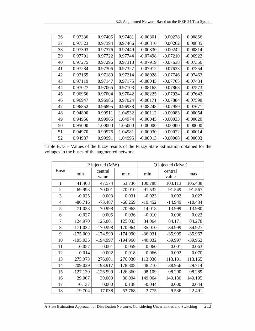
B.2. Augmented Network Based on the IEEE 24 Test System
A State Estimation Approach for Distribution Networks Considering Uncertainties and Switching 213
36 0.97330 0.97405 0.97481 -0.00301 0.00278 0.00856 37 0.97323 0.97394 0.97466 -0.00310 0.00262 0.00835 38 0.97303 0.97376 0.97449 -0.00330 0.00242 0.00814 39 0.97701 0.97722 0.97744 -0.07498 -0.07210 -0.06922 40 0.97275 0.97296 0.97318 -0.07919 -0.07638 -0.07356 41 0.97284 0.97306 0.97327 -0.07912 -0.07633 -0.07354 42 0.97165 0.97189 0.97214 -0.08028 -0.07746 -0.07463 43 0.97119 0.97147 0.97175 -0.08045 -0.07765 -0.07484 44 0.97027 0.97065 0.97103 -0.08163 -0.07868 -0.07573 45 0.96966 0.97004 0.97042 -0.08225 -0.07934 -0.07643 46 0.96947 0.96986 0.97024 -0.08171 -0.07884 -0.07598 47 0.96852 0.96895 0.96938 -0.08248 -0.07959 -0.07671 48 0.94890 0.99911 1.04932 -0.00112 -0.00083 -0.00054 49 0.94956 0.99965 1.04974 -0.00045 -0.00033 -0.00020 50 0.95000 1.00000 1.05000 0.00000 0.00000 0.00000 51 0.94970 0.99976 1.04981 -0.00030 -0.00022 -0.00014 52 0.94987 0.99991 1.04995 -0.00013 -0.00008 -0.00003
Table B.13 – Values of the fuzzy results of the Fuzzy State Estimation obtained for the voltages in the buses of the augmented network.
P injected (MW) Q injected (Mvar) Bus#
min central value
max min central value
max
1 41.408 47.574 53.736 100.788 103.113 105.438 2 69.993 70.001 70.010 91.532 91.549 91.567 3 -0.025 0.003 0.031 -0.023 0.002 0.027 4 -80.716 -73.487 -66.259 -19.452 -14.949 -10.434 5 -71.033 -70.998 -70.963 -14.018 -13.999 -13.980 6 -0.027 0.005 0.036 -0.010 0.006 0.022 7 124.970 125.001 125.033 84.064 84.171 84.278 8 -171.032 -170.998 -170.964 -35.070 -34.999 -34.927 9 -175.009 -174.999 -174.990 -36.031 -35.999 -35.967
10 -195.035 -194.997 -194.960 -40.032 -39.997 -39.962 11 -0.057 0.001 0.059 -0.060 0.001 0.063 12 -0.014 0.002 0.018 -0.066 0.002 0.070 13 275.973 276.001 276.030 113.038 113.101 113.165 14 -209.029 -193.917 -178.808 -48.210 -38.956 -29.714 15 -127.139 -126.999 -126.860 98.109 98.200 98.289 16 29.907 30.000 30.094 149.064 149.130 149.195 17 -0.137 0.000 0.138 -0.044 0.000 0.044 18 -19.704 17.038 53.768 -3.775 9.536 22.491
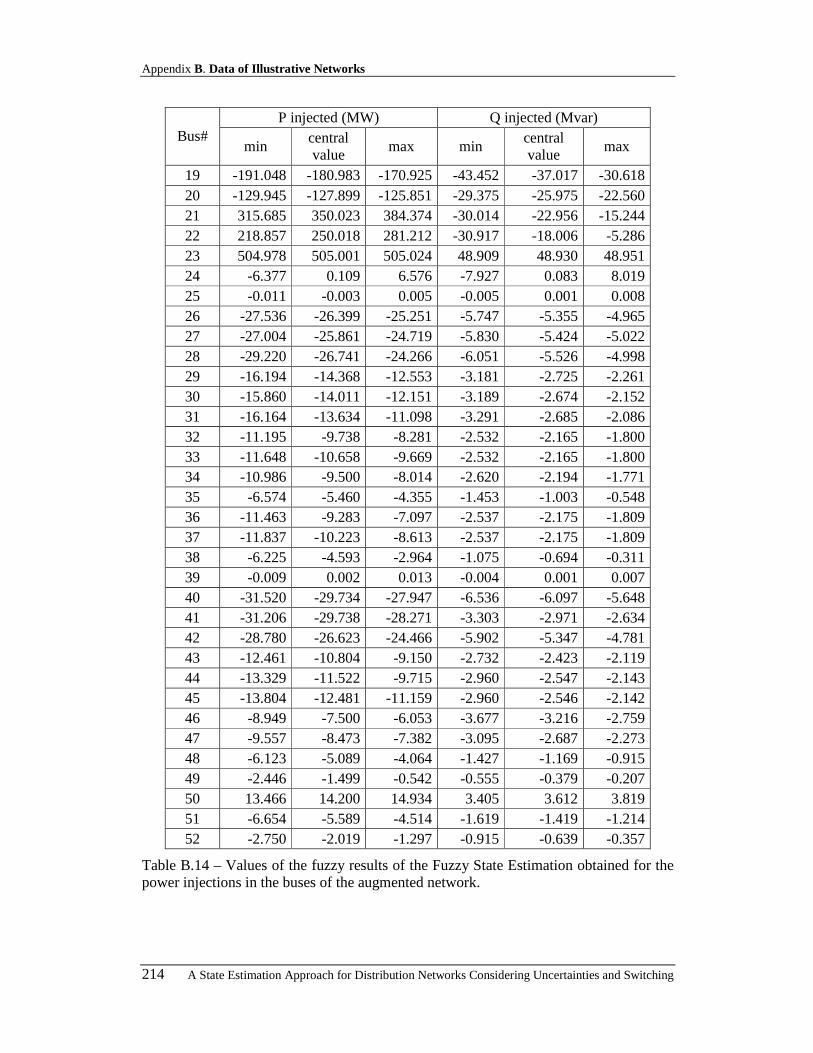
Appendix B. Data of Illustrative Networks
214 A State Estimation Approach for Distribution Networks Considering Uncertainties and Switching
P injected (MW) Q injected (Mvar) Bus#
min central value
max min central value
max
19 -191.048 -180.983 -170.925 -43.452 -37.017 -30.618 20 -129.945 -127.899 -125.851 -29.375 -25.975 -22.560 21 315.685 350.023 384.374 -30.014 -22.956 -15.244 22 218.857 250.018 281.212 -30.917 -18.006 -5.286 23 504.978 505.001 505.024 48.909 48.930 48.951 24 -6.377 0.109 6.576 -7.927 0.083 8.019 25 -0.011 -0.003 0.005 -0.005 0.001 0.008 26 -27.536 -26.399 -25.251 -5.747 -5.355 -4.965 27 -27.004 -25.861 -24.719 -5.830 -5.424 -5.022 28 -29.220 -26.741 -24.266 -6.051 -5.526 -4.998 29 -16.194 -14.368 -12.553 -3.181 -2.725 -2.261 30 -15.860 -14.011 -12.151 -3.189 -2.674 -2.152 31 -16.164 -13.634 -11.098 -3.291 -2.685 -2.086 32 -11.195 -9.738 -8.281 -2.532 -2.165 -1.800 33 -11.648 -10.658 -9.669 -2.532 -2.165 -1.800 34 -10.986 -9.500 -8.014 -2.620 -2.194 -1.771 35 -6.574 -5.460 -4.355 -1.453 -1.003 -0.548 36 -11.463 -9.283 -7.097 -2.537 -2.175 -1.809 37 -11.837 -10.223 -8.613 -2.537 -2.175 -1.809 38 -6.225 -4.593 -2.964 -1.075 -0.694 -0.311 39 -0.009 0.002 0.013 -0.004 0.001 0.007 40 -31.520 -29.734 -27.947 -6.536 -6.097 -5.648 41 -31.206 -29.738 -28.271 -3.303 -2.971 -2.634 42 -28.780 -26.623 -24.466 -5.902 -5.347 -4.781 43 -12.461 -10.804 -9.150 -2.732 -2.423 -2.119 44 -13.329 -11.522 -9.715 -2.960 -2.547 -2.143 45 -13.804 -12.481 -11.159 -2.960 -2.546 -2.142 46 -8.949 -7.500 -6.053 -3.677 -3.216 -2.759 47 -9.557 -8.473 -7.382 -3.095 -2.687 -2.273 48 -6.123 -5.089 -4.064 -1.427 -1.169 -0.915 49 -2.446 -1.499 -0.542 -0.555 -0.379 -0.207 50 13.466 14.200 14.934 3.405 3.612 3.819 51 -6.654 -5.589 -4.514 -1.619 -1.419 -1.214 52 -2.750 -2.019 -1.297 -0.915 -0.639 -0.357
Table B.14 – Values of the fuzzy results of the Fuzzy State Estimation obtained for the power injections in the buses of the augmented network.
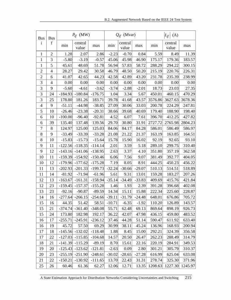
B.2. Augmented Network Based on the IEEE 24 Test System
A State Estimation Approach for Distribution Networks Considering Uncertainties and Switching 215
ifP (MW) ifQ (Mvar) ifI (A) Bus
i Bus
f min
central value
max min central value
max min central value
max
1 2 1.28 2.07 2.86 -2.23 -0.70 0.84 5.59 8.49 11.39 1 3 -5.80 -3.19 -0.57 45.06 45.98 46.90 175.17 179.36 183.57 1 5 45.61 48.69 51.78 56.94 57.83 58.72 288.29 294.22 300.15 2 4 28.27 29.42 30.58 46.79 48.50 50.20 215.19 220.76 226.31 2 6 41.07 42.65 44.23 42.58 42.89 43.20 231.78 235.39 238.99 3 4 0.00 0.00 0.00 0.00 0.00 0.00 0.00 0.00 0.00 3 9 -5.60 -4.61 -3.62 -3.74 -2.88 -2.01 18.73 23.03 27.35 3 24 -184.93 -180.84 -176.75 1.04 3.34 5.67 450.01 460.15 470.29 3 25 178.80 181.26 183.71 39.78 41.68 43.57 3576.86 3627.63 3678.36 4 9 -51.11 -44.98 -38.85 27.09 30.06 33.03 200.78 224.29 247.81 5 10 -26.46 -23.38 -20.31 38.66 39.68 40.69 179.40 188.90 198.40 6 10 -100.00 -96.40 -92.81 4.52 6.07 7.61 396.70 412.25 427.82 6 39 135.40 137.48 139.56 29.70 30.80 31.91 2727.72 2765.98 2804.23 7 8 124.97 125.00 125.03 84.06 84.17 84.28 586.01 586.49 586.97 8 9 -33.49 -33.39 -33.28 21.08 21.22 21.37 163.19 163.85 164.51 8 10 -15.83 -15.73 -15.64 15.78 15.90 16.02 92.19 92.65 93.10 9 11 -122.56 -118.35 -114.14 2.01 3.59 5.18 289.10 299.75 310.40 9 12 -143.16 -141.06 -138.95 2.63 3.37 4.10 351.80 357.19 362.58
10 11 -159.39 -154.92 -150.46 6.06 7.56 9.07 381.49 392.77 404.05 10 12 -179.96 -177.62 -175.28 7.19 8.05 8.91 444.25 450.23 456.22 11 13 -202.93 -201.33 -199.73 -32.24 -30.66 -29.07 510.13 514.51 518.89 11 14 -81.92 -71.94 -61.96 5.61 9.31 13.01 159.28 183.27 207.26 12 13 -163.67 -161.31 -158.94 -35.14 -34.49 -33.83 409.69 415.76 421.84 12 23 -159.45 -157.37 -155.28 1.46 1.93 2.39 391.28 396.68 402.08 13 23 -92.16 -90.87 -89.59 14.34 15.11 15.88 222.34 225.60 228.87 14 16 -277.64 -266.15 -254.66 -39.11 -31.79 -24.48 648.01 676.86 705.72 15 16 44.35 51.42 58.51 -10.71 -6.35 -1.92 110.20 126.89 143.57 15 21 -374.74 -361.40 -348.08 55.71 62.48 69.13 869.64 898.19 926.73 15 24 173.80 182.98 192.17 36.22 42.07 47.98 436.15 459.80 483.52 16 17 -255.71 -245.91 -236.12 37.46 44.28 51.14 590.47 611.92 633.40 16 19 45.72 57.50 69.29 30.99 38.11 45.24 136.96 168.93 200.94 17 18 -145.56 -132.02 -118.48 1.88 8.45 15.00 292.21 324.39 356.58 17 22 -127.03 -115.85 -104.68 14.57 20.50 26.47 262.23 288.49 314.79 18 21 -141.39 -115.29 -89.19 8.70 15.61 22.16 220.19 284.91 349.53 19 20 -125.43 -123.62 -121.81 -2.63 0.09 2.80 301.21 305.79 310.37 20 23 -255.19 -251.90 -248.61 -30.02 -28.65 -27.28 616.99 625.04 633.08 21 22 -150.21 -130.92 -111.65 13.70 22.43 31.31 278.74 325.30 371.96 25 26 60.46 61.36 62.27 12.06 12.71 13.35 1208.63 1227.30 1245.97

Appendix B. Data of Illustrative Networks
216 A State Estimation Approach for Distribution Networks Considering Uncertainties and Switching
ifP (MW) ifQ (Mvar) ifI (A) Bus
i Bus
f min central value
max min central value
max min central value
max
25 27 54.17 55.07 55.97 11.00 11.65 12.29 1083.80 1102.38 1120.95 25 28 63.89 64.82 65.75 13.12 13.78 14.42 1278.74 1297.91 1317.06 26 29 33.20 34.80 36.42 6.40 7.12 7.83 665.14 698.02 731.08 27 30 27.42 29.03 30.64 5.22 5.95 6.68 549.63 582.72 615.78 28 31 34.85 37.87 40.89 7.02 7.93 8.84 699.96 760.89 821.73 29 32 8.29 9.75 11.21 1.81 2.18 2.55 167.11 196.45 225.80 29 33 9.67 10.67 11.66 1.81 2.18 2.54 193.78 214.05 234.34 30 34 12.97 14.98 17.00 2.52 3.23 3.93 260.75 301.81 343.07 31 36 7.10 9.29 11.47 1.81 2.18 2.54 144.89 188.38 231.73 31 37 11.93 14.82 17.73 2.19 2.88 3.57 239.81 298.21 356.73 34 35 4.36 5.46 6.58 0.55 1.01 1.46 86.69 109.56 132.60 37 38 2.96 4.59 6.23 0.31 0.70 1.08 58.97 91.80 124.69 39 40 79.62 80.71 81.81 16.48 17.07 17.65 1604.38 1624.71 1645.04 39 41 55.67 56.77 57.86 11.09 11.67 12.26 1121.02 1141.32 1161.61 39 48 0.00 0.00 0.00 0.00 0.00 0.00 0.00 0.00 0.00 40 42 48.37 50.70 53.04 9.82 10.55 11.30 978.60 1024.35 1070.13 41 43 24.82 26.84 28.84 7.78 8.41 9.05 518.05 556.21 594.34 42 44 9.72 11.53 13.34 2.16 2.56 2.98 198.05 233.96 269.90 42 45 11.17 12.50 13.83 2.17 2.57 2.99 226.15 252.72 279.33 43 46 13.93 16.00 18.06 5.33 5.94 6.55 298.28 338.07 377.77 46 47 7.39 8.48 9.56 2.28 2.70 3.10 154.59 176.55 198.34 48 49 -6.12 -5.09 -4.06 -1.43 -1.17 -0.92 75.21 100.57 126.14 49 50 -7.98 -6.59 -5.20 -1.89 -1.55 -1.22 96.36 130.32 164.33 50 51 4.51 5.59 6.66 1.22 1.42 1.62 84.42 110.99 137.36 50 52 1.30 2.02 2.75 0.36 0.64 0.92 23.85 40.75 57.81
Table B.15 – Values of the fuzzy results of the Fuzzy State Estimation obtained for the power and current flows in the branches of the augmented network.