a static geometric medial axis domain decomposition in 2d ... · a static geometric medial axis...

A Static Geometric Medial Axis DomainDecomposition in 2D Euclidean Space

LEONIDAS LINARDAKIS and NIKOS CHRISOCHOIDES

College of William and Mary

We present a geometric domain decomposition method and its implementation, which producesgood domain decompositions in terms of three basic criteria: (1) The boundary of the subdomainscreate good angles, i.e., angles no smaller than a given tolerance Φ0, where the value of Φ0 isdetermined by the application which will use the domain decomposition. (2) The size of theseparator should be relatively small compared to the area of the subdomains. (3) The maximumarea of the subdomains should be close to the average subdomain area. The domain decompositionmethod uses an approximation of a Medial Axis as an auxiliary structure for constructing theboundary of the subdomains (separators). The N -way decomposition is based on the “divide andconquer” algorithmic paradigm and on a smoothing procedure that eliminates the creation of anynew artifacts in the subdomains. This approach produces well shaped uniform and graded domaindecompositions, which are suitable for parallel mesh generation.

Categories and Subject Descriptors: I.3.5 [Computer Graphics]: Computational Geometry andObject Modeling; J.6 [Computer-Aided Engineering]:

General Terms: Algorithms

Additional Key Words and Phrases: domain decomposition, parallel mesh generation, Delaunaytriangulation

1. INTRODUCTION

Although the Domain Decomposition (DD) problem has been studied for morethan 20 years in the context of parallel computing, there are many aspects of thisproblem which are unsolved. DD methods have been used for solving numericallypartial differential equations using parallel computing (cf. [Smith et al. 1996].Here we examine the Geometric Domain Decomposition problem (GDD) in thecontext of parallel mesh generation. We focus on the formulation, solution andimplementation of the GDD problem for a continuous 2-dimensional (2D) domainΩ into non-overlapping subdomains Ωi, so that the subdomains Ωi create no newartifacts, such as small angles between the separators ∂Ωi, and the separators and

This work was partially sponsored by the National Science Foundation under Grant No. 0049086,0085969. Funding support was also provided through the Virginia Institute of Marine Scienceand the Southeastern Universities Research Association under the grants ONR N00014-05-1-0831and NOAA NA04NOS4730254. Any opinions, findings, and conclusions or recommendationsexpressed in this material are those of the authors and do not necessarily reflect the views of theaforementioned institutes.Permission to make digital/hard copy of all or part of this material without fee for personalor classroom use provided that the copies are not made or distributed for profit or commercialadvantage, the ACM copyright/server notice, the title of the publication, and its date appear, andnotice is given that copying is by permission of the ACM, Inc. To copy otherwise, to republish,to post on servers, or to redistribute to lists requires prior specific permission and/or a fee.c© 2006 ACM 0098-3500/2006/1200-0001 $5.00

ACM Transactions on Mathematical Software, Vol. V, No. N, October 2006, Pages 1–26.

2 ·

Fig. 1. Left: Part of the Chesapeake bay geometry decomposed uniformly by the MADD method.The angles created by the separators are greater than 70. Right: Detail of the Delaunay meshof the decomposed geometry. The decompositions produced by the MADD are suitable for stableparallel graded mesh generation.

the external boundary ∂Ω. These decompositions are suitable for stable parallelgraded mesh generation procedures (see Fig. 1), where the termination of theseprocedures and the quality of the resulting elements depend on the features of thesubdomains. Furthermore, the same decompositions can be used for the next step,by the parallel FEM or FD solver. However, the geometric domain decompositionwe describe does not depend on how the mesh is used, or what is the PDE solvingmethod.

Parallel mesh generation methods decompose the original meshing problem intosmaller subproblems that can be solved (i.e., meshed) in parallel. There are twoapproaches that can be employed in order to decompose the problem: mesh datadecomposition and geometric domain decomposition techniques. Mesh data de-composition techniques compute data-subsets of the mesh that can be processedin parallel [Chrisochoides and Nave 2003; Kadow and Walkington 2003; Chernikovand Chrisochoides 2004]. The decomposition for these approaches is an easier prob-lem than the geometric domain decomposition problem, but communication andlocal synchronization are unavoidable during the parallel mesh generation in orderto maintain the conformity and quality of the distributed mesh.

Geometric domain decomposition techniques partition the domain into subdo-mains; the subdomains are created by inserting internal boundaries (separators)into the domain. Parallel mesh generation procedures that follow this approachrequire low communication [Chew et al. 1997], or no communication at all [Galtierand George 1996; Said et al. 1999; Linardakis and Chrisochoides 2006], and thusare very efficient. When communication is required by the parallel mesh generationprocedure, this will be analogous to the lengths of the separators. Hence, one of theACM Transactions on Mathematical Software, Vol. V, No. N, October 2006.

· 3

goals of the domain decomposition is to produce small separators. On the otherhand, the separators will be part of the geometry, and consequently part of thefinal mesh, so the decomposition has to meet certain quality criteria (like the sizeof the angles that it imposes), so that the quality of the mesh will not be distorted.

Geometric domain decomposition methods can be characterized as topology–basedor geometry–based. Typically topology–based techniques partition a mesh of thedomain, or the dual graph of a background mesh, giving a decomposition of thedomain. This approach is followed by the Metis library [Karypis and Kumar 1995b].On the other hand, geometry–based techniques take into account the geometriccharacteristics of the domain. For example, the Recursive Coordinate Bisectionapproach [Berger and Bokhari 1985] recursively bisects the domain along the axes,while the Inertial method [Nour-Omid et al. 1986] uses the inertia axis of the domainto produce a decomposition. Finally, libraries like Chaco [Hendrickson and Leland1995a] provide both topology and geometry-based approaches.

2. THE GEOMETRIC DOMAIN DECOMPOSITION PROBLEM

We examine the GDD problem in the context of parallel mesh generation. In the restof this paper we define as a domain Ω the closure of an open connected bounded setin R2. The boundary ∂Ω is defined by a planar straight line graph (PSLG), whichis formed by a set of line segments, intersecting only at their end points. Formallya 2-way domain decomposition is defined as follows. We assume the domain Ω isthe closure of an open connected bounded set and the boundary ∂Ω is a PSLGthat formed a set of linear segments which do not intersect1. A complete separatorH ⊆ Ω is a finite set of simple paths (a continuous 1-1 map h : [0, 1] → Ω), whichwe call partial separators, that do not intersect and define a decomposition Ω1,Ω2

of Ω, such that: Ω1 and Ω2 are connected sets, with Ω1 ∪ Ω2 = Ω, and for everypath P ⊂ Ω, which connects a point of Ω1 to a point of Ω2, we have P ∩H 6= ∅.

Guaranteed quality mesh generation algorithms [Chew 1989; 1993; Ruppert 1995]produce elements with good aspect ratio and good angles. These algorithms requirethat the initial boundary angles are within certain good bounds. For example,Ruppert’s algorithm [Ruppert 1995] requires boundary angles (the angles formed bythe boundary edges) no less than 60, in order to guarantee the termination. Whenthese algorithms are used in parallel, domain decomposition based, mesh generationprocedures, the separators are treated as external boundary of each subdomain. So,the domain decomposition should create separators that meet the requirements ofthe mesh generation algorithm. Therefore the constructed separator should formangles no less than a given bound Φ0, which is determined by the sequential meshgeneration procedure that will be used to mesh the individual subdomains. Even incases like [Triangle ], where a mesh generator can handle small input angles, theseangles are artifacts and will be permanent, distorting the quality of the final meshproduced by the parallel mesh generator.

The performance of the parallel mesh generation is affected by the required com-munication and the work-load balance among the processors. If there is com-munication, this is usually proportional to the size of the separator, therefore,

1This definition does not allow internal boundaries. The algorithm we present can be extendedto handle internal boundaries, if needed.

ACM Transactions on Mathematical Software, Vol. V, No. N, October 2006.

4 ·

Fig. 2. Left: The Pipe geometry. The angles produced by graph-based partitioners, like Metis,depend on the background mesh, and can be as small as the smaller angle of the mesh. The anglesmarked with dots are “small” (less than 60). Right: Part of the Chesapeake bay geometry. Whenthe geometry is complicated, methods like the Recursive Coordinate Bisection and the InertialMethod can produce arbitrary small angles between the separators and the domain boundary, andalso can place separators arbitrary close to the boundary.

one of our objectives in the domain decomposition step is to minimize the size ofthe separators. On the other hand, the load balancing problem is best addressedby over-decomposing the domain [Chrisochoides 1996]. Over-decomposition allowsboth static and dynamic load balancing methods to distribute equally the work-load among the processors more effectively [Barker et al. 2004; Linardakis andChrisochoides 2006]. These methods though will be less effective, if some of thesubdomains represent a much larger work-load than the average2. Therefore, weshould keep the maximum area of the subdomains close to the average subdomainarea3.

In conclusion, a geometric domain decomposition is suitable for stable parallelmesh generation, if it satisfies the following criteria.

C1. Create good angles, i.e., angles no smaller than a given tolerance Φ0 < π/2.The value of Φ0 is determined by the sequential, guaranteed quality, meshgeneration algorithm (for Ruppert’s algorithm we use the value Φ0 = 60).

C2. The length of the separator should be relatively small.C3. The maximum area of the subdomains should be close to the average subdo-

main area.

Previous DD approaches are very successful for traditional parallel PDE solvers,but they were not developed for parallel mesh generation procedures, and thus do

2Small work loads do not create load-balancing problems, on the contrary, the resulting granularitycan be used to improve the load balance, especially on heterogenous environments.3The area of the subdomains does not always reflect to work-load of the mesh generation proce-dure. However, for well shaped subdomains, as the ones produced by MADD, and Delaunay meshgenerators, the work-load is analogous to the area of the subdomain [Linardakis and Chrisochoides2006]


· 5

Fig. 3. Left: The Delaunay triangulation of the Pipe domain. The circumcenters of the trianglesapproximate the medial axis. Right: The circumcenters are the Voronoi nodes. The separator isformed by selecting a subset of the Voronoi nodes and connecting them with the boundary.

not address the problem of the formed angles. For example, graph based partition-ing algorithms, like Metis, give well-balanced decompositions with small separators,but the angles formed by the separators depend on the background mesh, and theycan be as small as the smallest angle of the mesh (see Figs. 2 Left, and 19). Onthe other hand, methods like the Recursive Coordinate Bisection and the InertialMethod can create arbitrary small angles, and also place the separators arbitraryclose to the boundary (see Fig. 2 Right), so they are unsuitable for parallel meshgeneration procedures. The geometric domain decomposition approach we presentaddresses all of the three above criteria, and is suitable for stable and efficientparallel mesh generation procedures.

3. MEDIAL AXIS DOMAIN DECOMPOSITION METHOD

The Medial Axis Domain Decomposition (MADD) method was first introducedin [Linardakis and Chrisochoides 2006] in the context of the Delaunay Decouplingmethod and it is based on an approximation of the medial axis (MA) of the do-main. The MA was introduced in [Blum 1967], and has been studied and utilizedextensively (cf. [Attali et al. ]. The approximation of the MA in the MADD methodis used as an auxiliary structure to determine separators that form good angles. Inthis paper we present an expanded and improved version of the MADD methodwhich includes a graded N-way domain decomposition procedure, and a smoothingprocedure for improving the quality of the separators.

A circle C ⊆ Ω is said to be maximal in a domain Ω, if there is no other circleC ′ ⊆ Ω such that C ( C ′. The closure of the locus of the circumcenters of allmaximal circles in Ω is called the medial axis Ω and will be denoted by MA(Ω).The intersection of the boundary of Ω and a maximal circle C is not empty. Thepoints C∩∂Ω, where a maximal circle C intersects the boundary, are called contactpoints of c, where c is the center of C. If b is a contact point of c, then theangles formed by the segment cb and the boundary are at least π/2 [Linardakis andChrisochoides 2006].

The medial axis of the domain can be approximated by Voronoi nodes of a dis-ACM Transactions on Mathematical Software, Vol. V, No. N, October 2006.

6 ·

external boundary Delaunay triangulation partial separators

a

a

a

2a3a

4

5

6

a1 a7

c

rejected separators

a

a

a

2a3a

4

5

6

a1 a7

c

Fig. 4. Left is a part of the Delaunay triangulation and right are the partial separators. Trianglea1a3a5 is a junction triangle, while the other triangles are not.

cretization of the domain [Brandt and Algazi 1992]. The Voronoi nodes are thecircumcenters of the Delaunay triangulation of the discretized domain (see Fig. 3right). As the Voronoi nodes approximate the MA, the segments that connect themto the boundary tend to create angles close to π/2. The approximation of MA(Ω)is achieved in two steps: (1) discretization of the boundary, and (2) computationof a boundary conforming Delaunay triangulation using the points from step (1).The circumcenters of the Delaunay triangles are the Voronoi nodes of the boundarypoints. The separators will be formed by either connecting these circumcenters totwo of the vertices of the Delaunay triangles, giving two segments, or from edgesof the Delaunay triangles, giving one segment. In both cases these segments arechosen so that they form good angles, with each other and the external boundary,and they are called partial separators. A complete separator will be formed by a setof one or more partial separators. Fig. 3 depicts the boundary conforming mesh ofthe cross section of a rocket and the medial axis approximation (left), and a 2-wayseparator for the same geometry (right).

Our goal is to create decompositions that form angles no less than a tolerance Φ0.The partial separators we choose are of two types (see Fig. 4): (a) non-boundaryedges of the Delaunay triangulation that form angles ≥ Φ0 with the boundary,and (b) segments that connect a triangle circumcenter with the triangle vertices.The first type of partial separator is easy to identify. We only have to scan thenon-boundary edges of the Delaunay triangulation and select the ones that createangles at least equal to our tolerance bound Φ0. In order to identify the secondtype of partial separator we define a special type of triangles. Let D be a Delaunaytriangulation of a discretization D of the boundary ∂Ω. We call a triangle t ∈ D ajunction triangle if:

(1) it includes its circumcenter c,(2) at least two of its edges are not in D,(3) at least two of the segments defined by the circumcenter and the vertices of t

form angles ≥ Φ0, both with the boundary and each other.

The second type of partial separators are included in junction triangles. In Fig. 4,ACM Transactions on Mathematical Software, Vol. V, No. N, October 2006.

· 7

triangle a1a3a5 satisfies all the above criteria and is a junction triangle. The othertriangles are not junction triangles. a1a2a3 and a1a5a6 do not include their circum-center and violate property (1); a3a4a5 has two edges on the boundary, violatingproperty (2); a1a6a7 does not include a partial separator that has acceptable an-gles (both angles at a1 and a7 are less than the tolerance Φ0, where Φ0 = 60),so it violates property (3). The partial separators are either internal Delaunayedges, like a1a2, a1a3 and a6a7, or are formed by connecting the circumcenter ofa junction triangle to its vertices. In our example a1ca3, a1ca5 and a3ca5 are thethree possible partial separators inside the junction triangle a1a2a3. The partialseparators always connect two points of the boundary, since D is a boundary con-forming triangulation. The complete separator is formed by choosing a subset ofpartial separators that will guarantee the decomposition of the geometry into twoconnected subdomains.

The existence and the quality of a complete separator depends on the numberand quality of the partial separators, which in turn depends on the level of thediscretization of the boundary segments. It is a difficult problem to pre-determinethe level of the refinement that would give an optimal decomposition. Increasingthe boundary refinement results a better approximation of the medial axis, andmore – and better in terms of the C1-C3 criteria – partial separators. However,over-refinement creates a number of problems. First, it increases the time for de-composing the geometry, since the time for creating the Delaunay triangulationdepends on the number of input points. Furthermore, it will take more time toidentify the partial separators and form a complete separator. Second, it couldresult into arithmetic rounding errors when calculating geometric entities, like cir-cumcenters and angles.

There are three parameters that effect the level of required refinement of theboundary: (1) the number of subdomains we want to create, (2) the characteristicsof the initial geometry, and (3) the angle lower bound Φ0. In our implementationwe compute a refining size based on the average length of the initial boundaryedges and on the square root of the number of subdomains (see Section 6). Theangle lower bound Φ0 can be as large as 80, depending on the geometry and therefining factor; for values larger than this the algorithm may not find a separatorthat satisfies the angle lower bound condition.

4. THE MADD ALGORITHM

The MADD algorithm uses as a starting point the approximation of the medialaxis by the Delaunay triangulation D, as described in the previous section. Anyalgorithm that gives a Delaunay boundary conforming triangulation can be used tocreate it. For our implementation we have used Triangle [Shewchuk 1996], which isconsidered to be a state of art Delaunay mesher for planar geometries. The MADDalgorithm uses the Delaunay triangulation to identify a set of candidate partialseparators. Then it will form a complete separator by a set of partial separators,that will guarantee the decomposition of the domain into two subdomains. Theselection of partial separators is based on minimizing the size of the separators,while maintaining the balance of the areas.

The MADD algorithm maps the Delaunay triangulation D into a graph GD,ACM Transactions on Mathematical Software, Vol. V, No. N, October 2006.

8 ·

external boundary Delaunay triangulation partial separators graph edges node contraction

a

a

a

2a3a

4

5

6

a1 a7

a

a

a

2a3a

4

5

6

a1 a7

a

a

a

2a3a

4

5

6

a1 a7

c

d

d

d

d

d d

d

1 1 12 2 2

3 3

4

5

7

d43

d

d

5

dd d d d d4d6d6

7

Fig. 5. An example of creating the MADD graph. Left is a part of the Delaunay triangulationand the creation of the corresponding initial graph GD. Center, the procedure of contracting thegraph by combining the vertices of GD. The vertices connected by doubled lines are combined.Right is the final graph G′

D that corresponds to this part.

which is a modified element dual graph. The information encapsulated in thisgraph includes: (a) the topology of D, (b) the length of the partial separators, and(c) the area of the subdomains that will be created. This information will be usedto : (1) guarantee that the inserted partial separators form a complete separator,(2) minimize the length of separators, and (3) keep the subdomain areas balanced.After GD is constructed, the graph is contracted, so that only the partial separatorsof D are represented as graph edges (see Section 4.2). Then the contracted graphis partitioned in a way that minimizes the cut cost and gives balanced subdomainweights. In our implementation we have used Metis [Karypis and Kumar 1995b],which is considered to be a state of art graph partitioner. Finally the graph parti-tion is translated back into insertions of partial separators, which results a 2-waydecomposition (see Section 4.3). The major steps of the algorithm are:

(1) Create a modified element dual graph GD from the Delaunay triangulation D.(2) Contract GD into the graph G′

D, so that only the candidate partial separatorsare represented as edges of G′

D.(3) Partition the graph G′

D, optimizing the cut-cost to subgraph weight ratio.(4) Translate the cuts of the previous partition into the corresponding partial sep-

arators and insert them into the geometry.

4.1 Construction of the Graph GD

In this step the junction triangles of the Delaunay triangulation D are dividedinto three triangles, and the final triangulation is represented as a weighted dualgraph. Each of the three triangles included into a junction triangle are representedby three graph vertices. Non-junction triangles are represented by a single graphvertex. Vertices that represent adjacent triangles are connected by a graph edge.The weight of each vertex is set equal to the area of the corresponding triangle,while the weight of a graph edge connecting two vertices is set equal to the lengthof the common triangle edge that is shared by the two corresponding triangles.

Fig. 5 (left) depicts the step for constructing the graph GD. Triangles a1a2a3,ACM Transactions on Mathematical Software, Vol. V, No. N, October 2006.

· 9

a1a5a6, a3a4a5 and a1a6a7 are not junctions, and each is represented by one vertex,d1, d6, d5, and d7 respectively. Triangle a1a3a5 is a junction triangle and is dividedin three triangles: a1ca3, a1ca5 and a3ca5, where c is the circumcenter of a1a3a5.These triangles are represented by the vertices d2, d4, and d3 respectively. Theweight of each vertex is equal to the area of the corresponding triangle. For example,the vertex d2 has weight equal to the area |a1ca3|. Vertices that represent adjacenttriangles are connected by a graph edge, with weight equal to the length of theircommon triangle edge. For example, the vertices d1 and d2 are connected by agraph edge with weight equal to the length |a1a3|, while the vertices for d2 and d3

are connected by a graph edge with weight equal to |ca3|. The above procedure isdescribed by Algorithm 1.

Algorithm 1.1. for all the triangles aiajak in D do2. if aiajak is a junction triangle then3. let c be the circumcenter of aiajak;4. create three vertices corresponding to triangles

aicaj , aicak, ajcak with weight equal to their areas;5. else6. create one vertex with weight equal to |aiajak|;7. endif8. endfor9. for all vertices d ∈ GD do

10. find the adjacent triangles and connect the correspondingvertices by a graph edge with weight equal to the length oftheir common triangle edge;

11. endfor

4.2 Graph Contraction

In this step the graph GD produced from the previous step is contracted into a newgraph G′

D, so that only the acceptable partial separators are represented as edges inG′D. In order to contract the graph GD we iterate through all the graph edges and

eliminate those that correspond to not acceptable triangle edges. A triangle edgeis not acceptable if at least one of the angles that it creates is less than Φ0. Thegraph edge that corresponds to non-acceptable triangle edges is deleted, and thetwo graph vertices that were connected by the eliminated edge are combined intoone vertex; the new vertex represents the total area of the triangles represented bythe contracted vertices.

Fig. 5 (center) illustrates the procedure of contracting the graph. The triangleedge a3a5 forms small angles with the boundary and is not acceptable. The corre-sponding graph edge d3d5 is eliminated, while the vertices d3 and d5 are combinedinto a new vertex. The new vertex represents the polygon a3ca5a4 and its weightis equal to the polygon area, which is the sum of the two previous areas. The newvertex also inherits all the external graph edges of the two previous vertices, which


10 ·

external boundary Delaunay triangulation partial separators graph edges node contraction

a

a

2a3a 5

6

a1 a7

c

4a

a

a

2a3a 5

6

a1 a7

4a

a

a

2a3a 5

6

a1 a7

4a

cd dd

d

d

d

d dd

d

dd

d

dd d d1 1 12 2 2

3 34

4 4

5 5

6 6

77

Fig. 6. An example of contraction of the vertices inside of a junction triangle. Left is a part ofthe Delaunay triangulation and the creation of the corresponding initial graph GD. Center, theprocedure of contracting the graph, in this case the two vertices of the junction triangle a1a3a5

are combined. Right is the final graph G′D and the corresponding candidate partial separators.

in this case are the two edges d3d4 and d2d3. The same procedure is followed foreliminating the edges d4d6 and d6d7. In Fig. 5 right the final graph G′

D is depictedwith the corresponding areas and partial separators.

In Fig. 6 we have a slightly different geometry, which depicts the elimination ofan internal edge of a junction triangle. The triangle edge ca3 forms a small anglewith the boundary, so it is not acceptable and it is eliminated. The two verticesd2 and d3 in the junction triangle a1a3a5, which are separated by this edge, arecombined into a new vertex. The new vertex inherits two graph edges connectingit to the same vertex d4. These two edges have a total weight equal to the lengthof the partial separator a1ca5. The above procedure is described by Algorithm 2.

Algorithm 2.1. for all edges didj ∈ GD do2. if the corresponding triangle edge

forms an angle < Φ0 then3. delete the edge didj ;4. create a new vertex d with weight equal to the

sum of the weights of the vertices di, dj ;5. transfer all the external graph edges of

di and dj to the new vertex d;6. endif7. endfor

4.3 The Construction of the Separator

The result of the previous step is a graph G′D, whose edges represent the partial

separators that can be used to decompose the domain. The next step is to partitionthe graph in two connected subgraphs and translate this partition into a geometricdomain decomposition.ACM Transactions on Mathematical Software, Vol. V, No. N, October 2006.

· 11

a

a

a

2a3a

4

5

6

a1 a7

a

a

a

2a3a

4

5

6

a1 a7

external boundary partial separators graph edges

c

a

a

a

2a3a

4

5

6

a1 a7

d 1 2

3

4

3

d1 4

d

dd2

d

d d

Fig. 7. Left is depicted the graph G′D with the corresponding areas. Center The graph is

partitioned by deleting two graph edges. Right The corresponding partial separator is insertedto the geometry.

The weights of the vertices of G′D represent the size of the corresponding areas,

while the weights of the edges represent the length of the corresponding partialseparators. The objective of the graph partitioner is to minimize the ratio of the cut-cost to the subgraph weight. The graph partitioning problem is challenging and hasbeen the source of good algorithms and software [Kernighan and Lin 1970; Barnardand Simon 1994; Hendrickson and Leland 1995b; 1995c; Karypis and Kumar 1995a;Walshaw et al. 1997], The graph contraction step, described in the previous section,has the additional merit of reducing significantly the size of the graph, resulting asmaller partitioning problem. In our implementation we have used Metis library ofgraph partitioning algorithms [Karypis and Kumar 1995b].

After partitioning the graph G′D into two connected subgraphs, the final step is

to construct the separator of the geometry, by translating the graph edge cuts toinsertions of partial separators. The partial separators, that correspond to edgescut by the graph partitioner, are inserted into the geometry. In Fig. 7 (left) thegraph G′

D is depicted, the graph partition cuts of the two edges d2d3 and d2d4

(middle), and the corresponding partial separator a1ca5 is inserted to the geometry(right). The construction of the separator is described in Algorithm 3.

Algorithm 3.1. for all the edges didj ∈ G′

D do2. if di and dj belong to different subgraphs then3. insert the partial separator, corresponding to didj ,

into the geometry;4. endif5. endfor

If the graph G′D has at least two vertices, then a 2-way partition exists and

it will give a decomposition of the domain into two subdomains (for the proofsee [Linardakis and Chrisochoides 2006]). Provided that the graph partitioner givesa small cut cost and balanced subgraph weights, the length of the separator will


12 ·

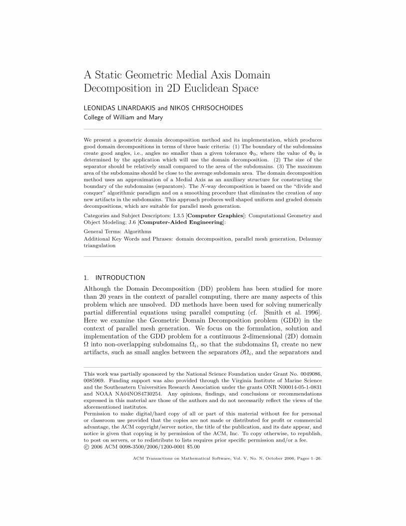
Fig. 8. N -way partitions, where N = 2, 4, 8, 16, by the MADD divide and conquer method.

be relatively small and the areas of the subdomains will be approximately equal.Moreover, since all the partial separators, by the construction of G′

D, form goodangles, the constructed separator will also form good angles. There are cases thoughwhere the graph partition will result the insertion of two partial separators thatmeet in the same boundary point. The angle formed between these two separatorsmight be less than the bound Φ0, giving a non-acceptable decomposition. We haveadded a routine that checks for these cases, modifies and repartitions the graph,so that only angles ≥ Φ0 are created during the insertion of separators. In generalthese cases correspond to high cut costs, due to the length of the two intersectingseparators, and in our experiments they rarely occured.

In summary, the constructed separator meets the decomposition criteria C1 - C3described in Section 2.

5. N-WAY DECOMPOSITION

The procedure described in the previous section decomposes the domain into twosubdomains, our goal though is to obtain much larger number of subdomains. N -way decompositions can be obtained by applying the MADD procedure recursively,in a divide and conquer way (see Fig. 8). In the first step the domain is decomposedinto two subdomains. Next, the largest subdomain is chosen and is decomposedagain into two subdomains. The procedure is repeated until we have created therequired number of subdomains. The N -way decomposition is described by Algo-rithm 4.

Algorithm 4.1. Read the definition of the domain Ω;2. Initialize and maintain a list of the subdomains;3. while the current number of subdomains is less than N do4. decompose the largest subdomain in two subdomains

using the MADD algorithm;5. update the list of the subdomains;6. endwhile

The recursive approach has both advantages and disadvantages. The MADDalgorithm is applied from scratch for every subdomain that is decomposed, so theACM Transactions on Mathematical Software, Vol. V, No. N, October 2006.

· 13

a bb

a

a

baa

ab

b

a

a

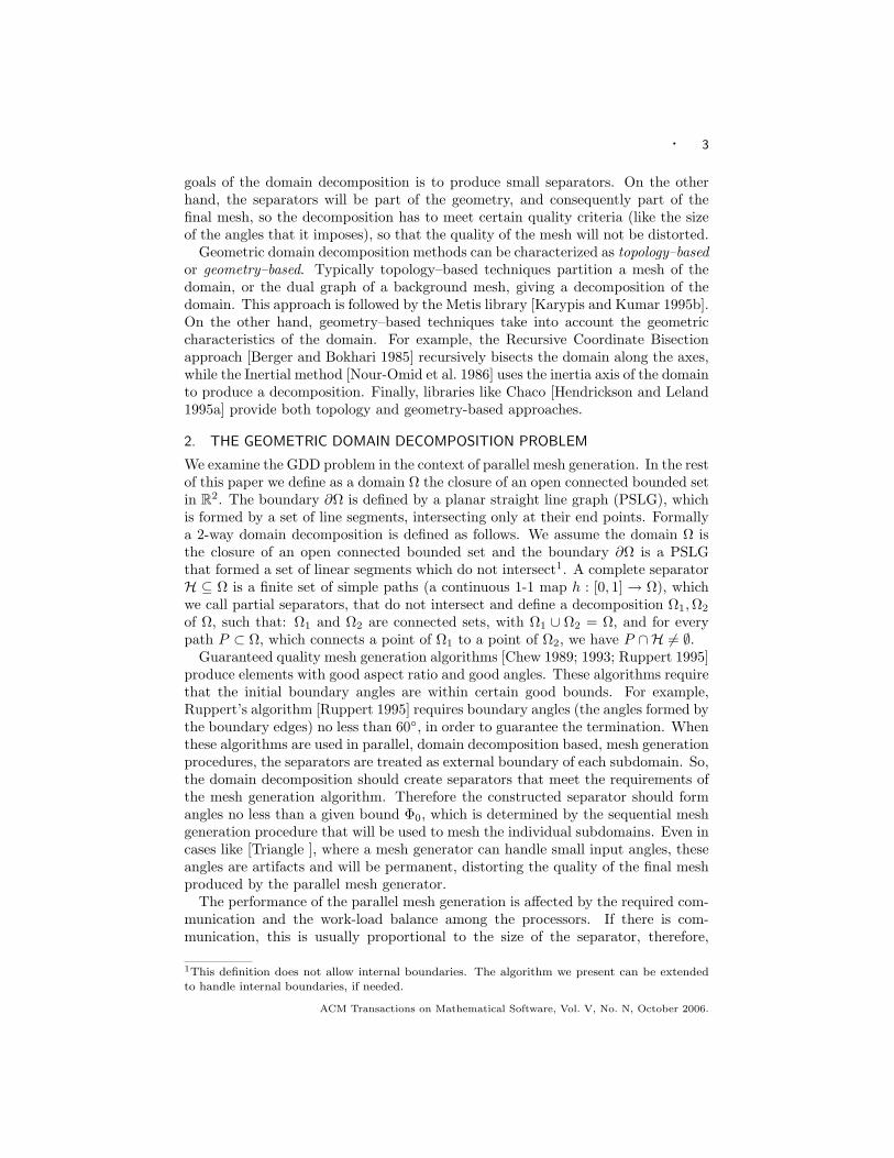
Fig. 9. The Pipe domain decomposed in 64 subdomains using the MADD algorithm. On the leftno smoothing is used. Most of the separators don’t meet at their end-points, and they create smallsegments on their common boundaries. On the middle the smoothing procedure is used, givingconforming separators. Right, the points of the first type (a) and second type (b) are depicted.

whole procedure, from the creation of the Delaunay triangulation to the graph par-tition and the insertion of separators, is repeated, discarding any previous informa-tion. Another disadvantage rises from the fact that each subdomain is decomposedindependently from the neighboring subdomain. This might cause the insertion ofseparators that create unnecessary small segments on their common boundary oftwo neighboring subdomains (see Fig. 9, left). In order to solve this problem weintroduce a smoothing procedure, which is described in Section 5.1.

The major advantage of the divide and conquer approach is that it adapts to thecurrent geometry. The Delaunay triangulation of the subdomains are re-calculated,after we insert the separators, incorporating the information of the so far decom-position. The new separators are formed taking into account the current shapeof the geometry. Fig. 8 demonstrates this fact. In contrast, if we used an N -waygraph partitioning approach, this information would not be avaliable, resulting poordecompositions.

5.1 Smoothing the Separators

One of the the disadvantages of independently decomposing each subdomain is thepossible creation of small features. The independent computation of the separatorsmight create small segments along their common boundary (see Fig. 9, left). Thesize of these segments depends on the level of the boundary refinement. As weincrease the number of segments, we also increase the probability of creating thesesmall segments. On the other hand, the graph partitioner has information onlyabout the size of the separators, and not about their quality, i.e., the angles thatthey form. Although all the permissible separators form angles greater than apredefined lower bound Φ0, we would like to choose the ones that are not onlysmall, but also form the best possible angles (that is near π/2). In order to dealwith these two issues we introduce a smoothing procedure that improves the qualityof the decomposition.

The smoothing procedure takes place in two steps. The first step takes placeduring the construction of the graph GD. In this step we incorporate into theweight of the graph edges two types of additional information: (a) the quality of


14 ·

the angles that the corresponding separators form, and (b) the conformity withexisting separators (i.e. if the separator’s end-points meet at the end-points of anexisting separator). The weight of each graph edge is multiplied by a coefficient f0,which reflects the quality of the minimum angle φ that the corresponding separatorforms. This coefficient is computed as f0 = 1

φ−Φ0+1 , for φ ≤ π/2, and 1π/2−Φ0+1 ,

for φ ≥ π/2. The coefficient f0 takes values from 1π/2−Φ0+1 , when φ ≥ π/2, up to

1, when the minimum angle is equal to the minimum acceptable bound φ = Φ0.So, the weight of the graph edge is decreased proportionally to the quality of theminimum angle.

We would also like to encourage the graph partitioner to choose separators thatconform with existing separators, i.e., that meet on the common boundary withthe existing partial separators of the adjacent subdomains. To this end we identifytwo types of boundary points (see Fig. 9, right). Points of the first type are eitherinitial points part of domain boundary, or are end-points of an existing separator.In order to encourage the graph partitioner to choose conforming separators, wedecrease the weight of the graph edges when these correspond to separators definedfrom points of the first type. These are end-points of existing separators (or ofthe initial boundary), and new separators that meet at these points are conformingwith the existing separators. The second type of points are the middle points ofsegments defined by the first type points. We also reduce the weight of the graphedges corresponding to separators defined from second type points. In this way weincrease the probability that a separator will be chosen that has end-points eitheron existing end-points (first type points), or away from them (second type points).

The previous step awards conforming separators, and the ones that form betterangles, but it does not guarantee that these will be chosen by the graph partitioner.In order to improve further the quality of the separator we introduce a secondsmoothing step, an ad hoc heuristic, after the graph partitioning procedure. Insteadof inserting the partial separators chosen by the graph partitioner, we examine allthe possible separators that are close to the initial ones, and insert the optimal,according to an optimality function. The neighboring separators are defined bythe neighboring points to the end-points of the initial separator. The optimalityfunction computes the degree of quality based on : (a) the size of the separator,(b) the minimum angle that it forms, and (c) the type of its end-points. Thecomputation of this function is similar as in the previous smoothing step.

The smoothing procedure, almost always, gives conforming separators that formgood angles. This depends though on the initial partition of the graph, the balanceof the decomposition, and of course, the geometric characteristics of the domain.

5.2 N-way Graded Decomposition

The procedure that we have described so far for N -way decompositions producesuniform domain decompositions, i.e. the areas of the subdomains are approximatelyequal. This approach is well suited for uniform mesh generation, but in many caseswe would like to have a graded, locally refined, mesh. Certain parts of the domain,where the model indicates higher activity, require smaller size of mesh elementsand thus a denser mesh. These parts could be determined in advance, based onthe properties of the geometry and the model, or as a result of an error estimationACM Transactions on Mathematical Software, Vol. V, No. N, October 2006.

· 15

Fig. 10. Graded MADD based on boundary weights. Left, a model of the Chesapeake bay isdecomposed in 1250 subdomains, with weights on all the boundary points and interpolation factorset to zero. Right, detail of the decomposition, the irregular inner polygons represent islands andare part of the initial domain.

function from a previous FEM procedure. The local mesh refinement procedurewill result disproportional mesh sizes for the subdomains that include these criticalareas. In order to maintain balanced memory requirements, and consequently work-load, during the mesh generation procedure, we have to follow a graded approachin creating the domain decomposition. The areas of the created subdomains shouldbe proportional to the expected mesh size, and the subdomains that require higherrefinement should be decomposed into smaller subdomains.

The problem of determining the element size, and thus the gradation of a mesh,has been studied extensively in the mesh generation and refinement literature (cf.[Borouchaki et al. 1997; Lohner 1997; Owen and Saigal 1997; Deister et al. 2004; Zhuet al. 2002]). Usually the size of the elements is computed as a function of: (a) thegeometry of the domain (curvature), (b) the distance from sources of activity in themodel (like heat sources), (c) a gradation control bound, and (d) error estimators,typically computed from a previous solution over a coarse mesh. In most cases abackground mesh and an interpolation procedure is employed to define the desiredelement size in each position of the domain.

In this section we describe a procedure that produces graded domain decompo-sitions. using the MADD method. There are two ways to define the gradation ofthe subdomains. The first is to define the required area for each subdomain. Thesecond is to assign a relative density weight for each subdomain, and use it as agradation criterion. While the first approach is a natural extension of the existingapproaches for defining the gradation of the mesh, it does not allow the user to pre-define the number of subdomains she wants to create. The number of subdomainsdepends not only on the expected size of the mesh, which can be estimated throughan area criterion, but also by the number of processors that we want to utilize andthe available memory. Using density weights allows us to produce graded decom-positions and at the same time to predefine the number of subdomains that will becreated.

N -way graded domain decompositions can be produced in a similar way as thenon-graded ones, by recursively applying the MADD procedure. The only step that


16 ·

needs to be modified is the way we choose the subdomain to be decomposed in line4 of Algorithm 4. In this step the subdomain with the greater area to required arearatio, or with the greater density weight, is chosen to be decomposed, instead of thesubdomain with the larger area. In the case of using the area ratio, no subdomainwith area ratio greater than a user-defined bound will be in the final decomposition.In the case of using a density weight criterion the parts of the geometry that havebeen assigned greater density weights will be decomposed more intensively, and thenumber of the created subdomains is predefined.

In our implementation the gradation of the decomposition can be controlled inthe following three ways:

(1) Using density weights on the boundary points.(2) Using density-weight or required-area values over an unstructured background

mesh.(3) Using a density-weight function or a required-area function over a structured

background grid.

Case (1). The use of density weights on the boundary points is the simplestcase, and can be viewed a sub-case of the case (2). We describe it separatelybecause it is simple to define, and in some cases (like crack propagation) we needa better refinement near the boundary. The weights assigned to the boundary aredefined in the PSLG file that describes the geometry. Each point, in addition toits coordinates, is assigned an integer density weight value. A value of zero meansthat the point will not contribute to the density. Each subdomain is assigned adensity weight value, which is the sum of its boundary weights. An interpolationfactor allows the user to define the weights of the created internal boundaries; weuse a linear interpolation procedure. An interpolation factor of zero will assign zeroweights to the interfaces. Examples of this approach are depicted in Fig. 10.

Case (2). In this case we use a density-weight or required-area background mesh.A set of points in the interior, or on the boundary, of the geometry is assigned ei-ther with density weights, which indicate the required level of refinement at theneighborhood of these points, or with required area values, which indicate the areaof the subdomain including this point. The points typically would be vertices of aprevious mesh (see Fig 12, left). The density weight of each subdomain is computedas the sum of the weights of the points included in the subdomain. An exampleof this approach is depicted in Fig. 11, which is a model used to study the incom-pressible turbulent flow past a circular cylinder [Dong and Karniadakis 2005], andin Fig. 12. The size of the background mesh should be proportional to the numbersubdomains we want to create. Creating a large number of subdomains using fewbackground points will result poor quality of the subdomain gradation, with muchlarger subdomains adjacent to small ones. This will increase the subdomain con-nectivity and the cost for the start-up in the communication of the FEM solver. Onthe other hand, too many background points will unnecessarily slow the procedure,without improving the quality of the gradation.

Case (3). In this case we use a density weight function, or a required area func-tion, to control the gradation of the decomposition. These functions are evaluatedACM Transactions on Mathematical Software, Vol. V, No. N, October 2006.

· 17

Fig. 11. Graded MADD based on weighted background mesh. Top is the weight backgroundmesh vertices of the Cylinder domain, and bottom is the corresponding decomposition in 280subdomains.

Fig. 12. Graded MADD based on weighted background mesh. Left is the weight background meshvertices of the Pipe domain, and right is the corresponding decomposition into 1250 subdomains.


18 ·

Fig. 13. Left, the Key is decomposed in 1250 subdomains using a linear weight function, propor-tional to x coordinate. Right, the Pipe decomposed in 1315 subdomains using an area functionproportional to ρ12, where ρ is the distance from the center of the inner circle.

over a structured gird created on the fly during the decomposition procedure. Thedensity-weight function assigns a weight to each point of the created backgroundmesh, and, as in case (2), the density weight of each subdomain is computed as thesum of these weights. An example of this approach is depicted in Fig. 13 (left).

The required-area function assigns to each point the maximum subdomain areathat is expected for the subdomain that includes this point. The required-area for asubdomain is computed as the minimum of the required-area function values of allthe mesh points contained in the subdomain. In each step the subdomain with thehighest ratio of area over required area is chosen to be decomposed. The procedureis repeated, until no ratio is greater than a user-defined bound (default is 1), oruntil a maximum number of subdomains is reached. An example of this approachis depicted in Fig. 13 (right).

6. IMPLEMENTATION

The programming language for our implementation is ANSI C++, and the wholelibrary is encapsulated into the madd class. The [Triangle ] library ([Shewchuk1996]) was used for the creation of the Delaunay triangulation during the MADDprocedure. Also, the [Metis ] library ([Karypis and Kumar 1995b]) was used for thegraph partitioning step in the MADD procedure. The MADD method requires agraph partition into two connected subgraphs; we implemented a routine that re-stores the connectivity in the cases where Metis returns non-connected components.All the libraries where used without modifications.

The basic methods are described in Table I, a detailed description is providedin the source program. The libraries for the area and weight function are loadeddynamically through the ld dynamic linker. The file format (.poly) of the domainsis the same as in [Triangle ], and describes the domain in three sections: (a) a set ofboundary points in x y coordinates, (b) a set of segments, in 〈endpoint1〉〈endpoint2〉form, and (c) a set of holes in x y coordinates. The file format of the decomposi-tions is similar. It describes the decomposition in four sections: (1) a set of points,(2) a set of segments, (3) a set of subdomains defined by segments of section (2),and (4) a set of holes for each subdomain. Examples of files are provided with thesoftware.ACM Transactions on Mathematical Software, Vol. V, No. N, October 2006.

· 19

readPolyFile(char* name) Reads a poly file (the initial domain).

decompose(int subDomains) The main decomposition routine.

readBackgroundWeights(char* name) Reads weighted background mesh nodes from a file.

readBackgroundAreas(char* name) Reads area background mesh nodes from a file.

writePolyFileAll(char* fileName) Writes all the subdomains to different poly files.

writeSubdomainFile(char* name) Writes the decomposition in points, segments, and

subdomains - segments.

setWeightFunction(char *libraryName, Sets the weight function.

char *functionName)

setAreaFunction(char *libraryName, Sets the area function.

char *functionName)

setPhi(double phiValue) Sets minimum acceptable angle formed during the decomposition.

setDecAreaRatio(double ratioValue) Sets the min area ratio for decomposing a subdomain.

setUniformRefineLevel(double uniformValue) Sets the uniform refining and

decomposition factor.

setAdaptiveRefineLevel(double adaptiveValue) Sets the graded refining and

decomposition factor.

setMaxImbalanceLevel(double imbalanceValue) Sets the maximum acceptable imbalance

during the madd partition.

setMaxSmoothLevel(int smoothLevel) Defines the number of the smoothing iterations.

setInterpolationWeightLevel(double weightValue) Sets the interpolation coefficient

for the weights of new points.

Table I. The basic methods of the madd class.

A line command user interface is provided with the library. This interface pro-gram (maddi) can receive and execute a number of simple commands; the basiccommands are are described in Table II. An example of a set of commands is:

read pipe.polyset f=0.35dec 400write pipe400.polywriteSubdomains pipe400.datexit

The user can set a number of optional parameters, through the set command,that controls various functional aspects, like the level of refinement, the level ofsmoothing, balancing, etc. The basic parameters are described in Table III.

The level of refinement is based on a user-defined uniform refinement factor r,and the

√N , where N are the number of subdomains. The square root function

of the number of subdomains was chosen in a heuristic way, based on the factthat the square of the lengths of the separators is analogous to the areas of thesubdomains. The average area of subdomain is A/N , where A is the total area andN the number of subdomains. So, the separator lengths will be proportional to√

1/N , and consequently the level of refinement should be analogous to√

N . Therefinement level, and the decomposition times, for the Pipe and the Chesapeakebay tend to reflect this “square root” behavior. This is not the case for the Key,which has few initial segments, and requires more intense refinement in order to getgood decompositions. The refinement factor r defines a uniform refinement level,


20 ·

read <filename> Reads a poly file.

dec [<noOfSubdomains>] Decomposes the doamin.

write <filename> [all] Writes the decomposed poly file.

read_weights <filename> Reads weighted background mesh nodes from a file.

read_areas <filename> Reads area background mesh nodes from a file.

writeSubdomains <filename> Writes the decomposition into a file.

setWeightFunction <libraryName> <functionName> Sets the weight function.

setAreaFunction <libraryName> <functionName> Sets the area function.

set <parameter>=<value> Sets the <value> to the <parameter>.

exit Exits.

Table II. The basic commands for the maddi interface.

for example, if a boundary segment is to be divided to four subsegments, a factorr = 2 will cause it to be divided into 8 subsegments. In all our experiments thevalues for r were between 2 and 4. The gradation factor a controls the level ofgradation, in association with the uniform refinement factor r. The total densityweight of the subdomain is computed as

r × subdomain area + a× subdomain weight.

In this way the relation between a and b controls the intensity of the gradation.

7. EXPERIMENTAL RESULTS

For our experiments we used three model domains. The Pipe model is an approx-imation of a cross section of a regenerative cooled pipe geometry. It consists of576 boundary segments and 9 holes. The Key is a domain provided with Trian-gle [Shewchuk 1996], and has 54 boundary segments and 1 hole. The Chesapeakebay (Cbay) model defined from 13,524 points and it has 26 islands.

We ran three sets of experiments. In the first set of experiments we produceduniform decompositions for the three test domains. In the second set of experi-ments we produced graded decompositions, using the three approaches describedin Section 5.2: (a) we used weights on the boundaries to produce graded decompo-sitions, (b) we experimented using weight and area background meshes, and (c) weused weight and area functions over structured grids. The above experiments wereperformed on a a Pentium IV 3GHz processor, and we used a lower angle boundof f = 0.3333 rads (≈ 60). A third set of experiments was performed in order toasses the quality and efficiency of the MADD and compare it to Metis, which is astate of the art graph partitioner. For these experiments we decomposed the Keygeometry, using a Dual Pentium 3.4GHz processor.

Our results show that the time to decompose a domain is directly related tothe size of the domain (measured in number of segments), and the level of therefinement we apply on it (see Figs. 14 -15). The problem size for all the majorroutines (Delaunay triangulation, graph creation and partition) is proportional tothe number of the input segments, and thus we should expect this behavior. Thelevel of refinement is analogous to

√N , where N are the number of subdomains.

The refinement level, and the decomposition times, for the Pipe and the Chesapeakebay tend to reflect this “square root” behavior. This is not the case for the Key,ACM Transactions on Mathematical Software, Vol. V, No. N, October 2006.

· 21

f Defines the minimum angle bound created by the separators (in rads).r Defines the uniform refinement level. The expected length of the segments, after

refining, is multiplied by 1/r. Equivalently, the number of the segments after refiningis multiplied by r.

a The gradation factor for density weights. The density weight of the subdomains ismultiplied by a, while the area is multiplied by the uniform refinement level r. Thetotal sum gives the density weight of the subdomain.

p The interpolation factor for density weights. The weights of the new points of theseparators are computed by linear interpolation of the weights of the separator endpoints, multiplied by p. A value p = 0 eliminates the weights on the separators.

i The level of acceptable imbalance during the smoothing. The values should be be-tween 0.6 and 0.9 (default is 0.75).

Table III. The basic parameters used in the set command.

which has few initial segments, and requires more intense refinement in order toget good decompositions.

For the first group of graded decomposition experiments we used boundaryweights on the three domains. The user can control the gradation level, by set-ting a gradation factor a, and the weight interpolation, p, that will be applied onthe interfaces. The parameters for the Pipe and the Key were r = 3, a = 3, p = 0.5,while for the Cbay they were r = 2, a = 3, p = 0. One of the difficulties for decom-posing a geometry based on boundary weights (and also weight or area functions)is that the boundary refinement will have to be adaptive on the local weights. Inour implementation, segments that have greater weight will be refined more. Thesedifficulties can be solved by a computing on the fly, locally and independently, thelevel of refinement required for each subdomain.

The second group of experiments was performed on the Pipe domain using abackground mesh of 1,010 points. Both area and weight values over the backgroundmesh were used, and they produced similar decompositions for the same number ofsubdomains (see Fig. 12). The quality of the gradation depends on the ratio of thenumber of mesh points to the number of subdomains, as well as the gradation ofthe background mesh. Domain decomposition into a large number of subdomains,while using a small number of background mesh points, will result poor gradation.

We also tested the Pipe and the Key domains using weight and area functions,evaluated over a structured grid. This grid is created on the fly, when each subdo-main is created; it includes a total of 21,684 points for the Pipe domain and 8,115points for the Key. This high number of the points results in a good approximationof the density for each subdomain (the decompositions are depicted in Fig. 13),while the cost to create them is small (see Fig. 17). Of course, defining the func-tions analytically has the advantage of avoiding the interpolation procedure, whichcan have a significant cost. The weight and area functions are defined by the userand are linked dynamically, during the execution of the program.

For the third set of experiments we partitioned the Key geometry up to 2,000subdomains uniformly, and we compare the results obtained by MADD to thoseobtained by Metis. For the Metis decompositions we created background Delaunaymeshes of size approximately 120 triangles per subdomain, The Delaunay meshgeneration procedure is the only one that provides quality guarantees, creating


22 ·

0 200 400 600 800 1000 1200

Subdomains

0

0.2

0.4

0.6

0.8

1

1.2

1.4

1.6

1.8

2

2.2

2.4

2.6

Tim

e (s

ecs)

PipeKeyCBay

Fig. 14. Decomposition times for the uniformMADD.

0 200 400 600 800 1000 1200

Subdomains

0

5000

10000

15000

20000

Ref

inem

ent (

segm

ents

)

PipeKeyCh. bay

Fig. 15. The refinement (number of segments)for the uniform decompositions

angles no less than 30. The background mesh was translated into a weightedgraph, with weights reflecting the edge lengths and the triangle areas. For theMADD we used an adaptive local refinement approach to produce the Medial Axisapproximation. The lower angle bound was set to 70.

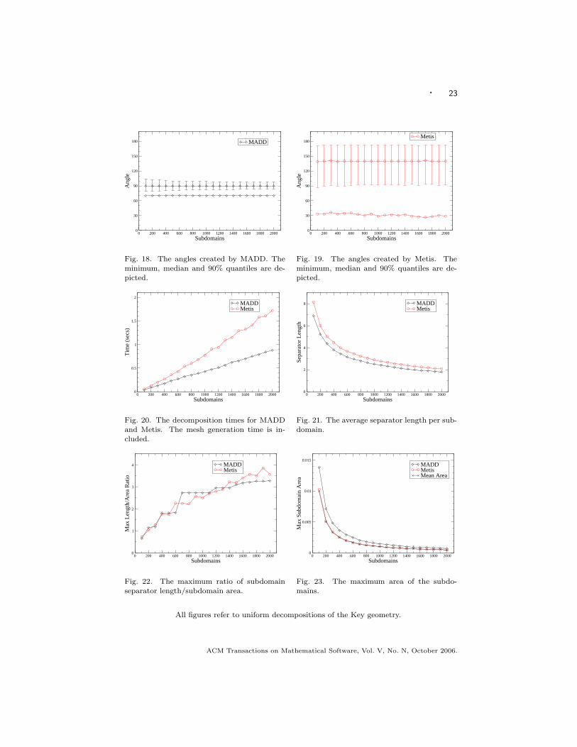
Figure 18 depicts the minimum, median and 90% quantiles of the angles createdby MADD. As expected, the minimum angles are no less than 70, while most ofthe angles are close to 90. In comparison, Metis gives minimum angles as smallas the ones in the background mesh (see Fig. 19). The efficiency of the MADDdepends on the geometry (Fig. 14), while the efficiency of Metis depends on thesize of the background mesh. For the Key geometry MADD performs better (seeFig. 20), for the Pipe the decomposition times had small differences, while for theCbay domain Metis performed better. The average length of the separators persubdomain is almost the same (Fig. 21), with MADD being slightly better. Themaximum ratio of the subdomain separator length to the subdomain area is thesame for the two methods, see Fig. 22. The maximum subdomain area is close tothe average subdomain area for the MADD method (Fig 23), while Metis resultsalmost perfect maximum subdomain area due to the near perfect balancing that it

0 200 400 600 800 1000 1200

Subdomains

0

0.2

0.4

0.6

0.8

1

1.2

1.4

1.6

1.8

2

2.2

2.4

2.6

Tim

e (s

ecs)

PipeKeyCBay

Fig. 16. Decomposition times for the weightedboundary MADD.

0 200 400 600 800 1000 1200

Subdomains

0

0.2

0.4

0.6

0.8

1

1.2

1.4

1.6

1.8

2

2.2

2.4

2.6

Tim

e (s

ecs)

Pipe (weight mesh)Pipe (weight function)Key (weight function)

Fig. 17. Decomposition times for the gradedMADD using a weighted background mesh andweight functions.


· 23

0 200 400 600 800 1000 1200 1400 1600 1800 2000

Subdomains

0

30

60

90

120

150

180

Ang

le

MADD

Fig. 18. The angles created by MADD. Theminimum, median and 90% quantiles are de-picted.

0 200 400 600 800 1000 1200 1400 1600 1800 2000

Subdomains

0

30

60

90

120

150

180

Ang

le

Metis

Fig. 19. The angles created by Metis. Theminimum, median and 90% quantiles are de-picted.

0 200 400 600 800 1000 1200 1400 1600 1800 2000

Subdomains

0

0.5

1

1.5

2

Tim

e (s

ecs)

MADDMetis

Fig. 20. The decomposition times for MADDand Metis. The mesh generation time is in-cluded.

0 200 400 600 800 1000 1200 1400 1600 1800 2000

Subdomains

0

2

4

6

8Se

para

tor

Len

gth

MADDMetis

Fig. 21. The average separator length per sub-domain.

0 200 400 600 800 1000 1200 1400 1600 1800 2000

Subdomains

0

1

2

3

4

Max

Len

gth/

Are

a R

atio

MADDMetis

Fig. 22. The maximum ratio of subdomainseparator length/subdomain area.

0 200 400 600 800 1000 1200 1400 1600 1800 2000

Subdomains

0

0.005

0.01

0.015

Max

Sub

dom

ain

Are

a

MADDMetisMean Area

Fig. 23. The maximum area of the subdo-mains.

All figures refer to uniform decompositions of the Key geometry.


24 ·

produces.

8. CONCLUSIONS AND FUTURE WORK

We propose a geometric domain decomposition method, based on the Medial Axis,which produces good domain decompositions in terms of three basic criteria: (1) Theinternal boundary of the subdomains forms good angles, i.e., angles no smaller thana given tolerance Φ0. (2) The size of the separator is relatively small compared tothe area of the subdomains. (3) The maximum area of the subdomains is closeto the average subdomain area. The resulting decompositions do not create newartifacts in the geometry and are suitable for stable and efficient parallel meshgeneration procedures. The MADD can also create graded decompositions, basedon density grids, or density functions; these decompositions are useful for gradedparallel mesh generation. The experimental data demonstrate that the method isefficient, generating more than a thousand subdomains in less than two seconds,and effective, resulting angles close to 90 and small length of separators.

Although it is straight forward to extend the MADD algorithm to three dimen-sions, using a tetrahedral Delaunay mesh, there are no guarantees of the quality ofthe resulting decomposition. The Voronoi points of the refinement do not convergeto the Medial Axis in three dimensions, and the formed angles are not guaranteedto be close to 90. However, we believe that the Medial Axis can be a useful toolfor geometric domain decompositions in three dimensions, and this is a subject offuture work.

ACKNOWLEDGMENTS

Two basic software libraries were used by our software: [Triangle ], by JonathanShewchuk, for the Delaunay triangulation, and [Metis ], by George Karypis et al.,as the graph partitioner. We thank them for kindly providing these libraries. Thecopyright and rights of use, for [Triangle ] and [Metis ] are as stated in the respectivesoftware; the user interested in using MADD should download these two librariesdirectly form their web sites, observing the conditions of use stated there and intheir source code. [Showme ] and [mview ] were used to produce the figures of thedomains in this paper.

We would like to thank Professor Harry Wang and Dr. Mac Sisson from VirginiaInstitute of Marine Science for providing the data for the shoreline of the Chesa-peake bay. Finally, we would like to thank the anonymous referees for their veryuseful suggestions, which improved this paper.

REFERENCES

Attali, D., Boissonnat, J.-D., and Edelsbrunner, H. Stability and computation of the medialaxis — a state-of-the-art report. In Mathematical Foundations of Scientific Visualization,Computer Graphics, and Massive Data Exploration.

Barker, K., Chrisochoides, N., Chernikov, A., and Pingali, K. 2004. A load balancingframework for adaptive and asynchronous applications. IEEE Trans. Parallel and DistributedSystems 15, 2 (Ferbruary), 183–192.

Barnard, S. T. and Simon, H. D. 1994. A fast multilevel implementation of recursive spectralbisection for partitioning unstructured problems. Concurrency: Practice and Experience 6,101–107.


· 25

Berger, M. and Bokhari, S. 1985. A partitioning strategy for pdes across multiprocessors. InProceedings of the 1985 International Conference on Parallel Processing.

Blum, H. 1967. A transformation for extracting new descriptors of shape. In Models for thePerception of speech and Visual Form. MIT Press, 362–380.

Borouchaki, H., George, P. L., Hecht, F., Laug, P., and Saltel, E. 1997. Delaunay meshgeneration governed by metric specifications, Part I. Algorithms and Part II. Applications.Finite Elements in Analysis and Design 25, 61–83 and 85–109.

Brandt, J. W. and Algazi, V. R. 1992. Continuous skeleton computation by Voronoi diagram.Comput. Vision, Graphics, Image Process. 55, 329–338.

Chernikov, A. and Chrisochoides, N. 2004. Practical and efficient point insertion schedulingmethod for parallel guaranteed quality Delaunay refinement. In Proceedings of the 18th annualinternational conference on Supercomputing. Malo, France, 48–57.

Chew, L. P. 1989. Guaranteed quality triangular meshes. Tech. Rep. TR-89-983, Department ofComputer Science, Cornell University.

Chew, L. P. 1993. Guaranteed-quality mesh generation for curved surfaces. In 9th AnnualSymposium on Computational Geometry. ACM, San Diego, California, 274–280.

Chew, L. P., Chrisochoides, N., and Sukup, F. 1997. Parallel constrained Delaunay triangula-tion. In ASME/ASCE/SES Special Symposium on Trends in Unstructured Mesh Generation.Evanston, IL, 89–96.

Chrisochoides, N. 1996. Multithreaded model for the dynamic load-balancing of parallel adaptivepde computations. Applied Numerical Mathematics 20, 349–365.

Chrisochoides, N. and Nave, D. 2003. Parallel Delaunay mesh generation kernel. InternationalJournal for Numerical Methods in Engineering 58, 2, 161–176.

Deister, F., Tremel, U., Hasan, O., and Weatherill, N. P. 2004. Fully automatic and fastmesh size specification for unstructured mesh generation. Engineering with Computers 20,237–248.

Dong, S. and Karniadakis, G. 2005. DNS of flow past a stationary and oscillating rigid cylinderat re = 10,000. Journal of Fluids and Structures 20(4), 519–531.

Galtier, J. and George, P.-L. 1996. Prepartitioning as a way to mesh subdomains in parallel.In 5th International Meshing Roundtable. Pittsburgh, Pennsylvania, 107–122.

Hendrickson, B. and Leland, R. W. 1995a. The Chaco user’s guide version 2.0. Tech. rep.,Sandia National Laboratories.

Hendrickson, B. and Leland, R. W. 1995b. An improved spectral graph partitioning algorithmfor mapping parallel computations. SIAM Journal on Scientific Computing 16, 2, 452–469.

Hendrickson, B. and Leland, R. W. 1995c. A multi-level algorithm for partitioning graphs. InSupercomputing. San Diego, CA.

Kadow, C. and Walkington, N. 2003. Design of a projection-based parallel Delaunay meshgeneration and refinement algorithm. In 4th Symposium on Trends in Unstructured MeshGeneration.

Karypis, G. and Kumar, V. 1995a. A fast and high quality multilevel scheme for partition-ing irregular graphs. Tech. Rep. TR 95-035, Department of Computer Science, University ofMinnesota, Minneapolis.

Karypis, G. and Kumar, V. 1995b. MeTis: Unstructured Graph Partitioning and Sparse MatrixOrdering System, Version 2.0.

Kernighan, B. W. and Lin, S. 1970. An efficient heuristic procedure for partitioning graphs.Bell Systems Technical Journal 49(2), 291–307.

Linardakis, L. and Chrisochoides, N. 2006. Delaunay Decoupling Method for parallel guaran-teed quality planar mesh refinement. SIAM Journal on Scientific Computing 27, 4, 1394–1423.

Lohner, R. 1997. Automatic unstructued grid generators. Finite Elements in Analysis andDesign 25, 111–135.

Metis. http://www-users.cs.umn.edu/~karypis/metis/index.html.

mview. http://mview.sourceforge.net/.


26 ·

Nour-Omid, B., Raefsky, A., and Lyzenga, G. 1986. Solving finite element equations onconcurrent computers. American Soc. Mech. Eng, 291–307.

Owen, S. J. and Saigal, S. 1997. Neighborhood-based element sizing control for finite elementsurface meshing. 6th International Meshing Roundtable.

Ruppert, J. 1995. A Delaunay refinement algorithm for quality 2-dimensional mesh generation.J. Algorithms 18, 3, 548–585.

Said, R., Weatherill, N., Morgan, K., and Verhoeven, N. 1999. Distributed parallel Delaunaymesh generation. Comp. Methods Appl. Mech. Engrg. 177, 109–125.

Shewchuk, J. R. 1996. Triangle: Engineering a 2D quality mesh generator and Delaunay tri-angulator. In Applied Computational Geometry: Towards Geometric Engineering, M. C. Linand D. Manocha, Eds. Lecture Notes in Computer Science, vol. 1148. Springer-Verlag, 203–222.From the First ACM Workshop on Applied Computational Geometry.

Showme. http://www.cs.cmu.edu/~quake/showme.html.

Smith, B., Bjrstad, P., and Gropp, W. 1996. Domain decomposition: parallel multilevel methodsfor elliptic partial differential equations. Cambridge University Press, 1996., New York.

Triangle. http://www.cs.cmu.edu/~quake/triangle.html.

Walshaw, C., Cross, M., and Everett, M. G. 1997. Parallel dynamic graph partitioning foradaptive unstructured meshes. Journal of Parallel and Distributed Computing 47, 2, 102–108.

Zhu, J., Blacker, T., and Smith, R. 2002. Background overlay grid size functions. In 11thInternational Meshing Roundtable. Sandia National Laboratories, 65–74.


a static geometric medial axis domain decomposition in 2d ... · a static geometric medial axis...

Documents