a statistical model to explain the mendel fisher controversy · pdf filea statistical model to...

arX

iv:1

104.

2975

v1 [

stat

.ME

] 1

5 A

pr 2

011

Statistical Science

2010, Vol. 25, No. 4, 545–565DOI: 10.1214/10-STS342c© Institute of Mathematical Statistics, 2010

A Statistical Model to Explain theMendel–Fisher ControversyAna M. Pires and Joao A. Branco

Abstract. In 1866 Gregor Mendel published a seminal paper contain-ing the foundations of modern genetics. In 1936 Ronald Fisher pub-lished a statistical analysis of Mendel’s data concluding that “the dataof most, if not all, of the experiments have been falsified so as to agreeclosely with Mendel’s expectations.” The accusation gave rise to a con-troversy which has reached the present time. There are reasonablegrounds to assume that a certain unconscious bias was systematicallyintroduced in Mendel’s experimentation. Based on this assumption, aprobability model that fits Mendel’s data and does not offend Fisher’sanalysis is given. This reconciliation model may well be the end of theMendel–Fisher controversy.

Key words and phrases: Genetics, ethics, chi-square tests, distributionof p-values, minimum distance estimates.

1. INTRODUCTION

Gregor Mendel is recognized as a brilliant scientistand the founder of modern genetics. However, longago, another eminent scientist, the statistician andgeneticist, Sir Ronald Fisher, questioned Mendel’sintegrity claiming that Mendel’s data agree betterwith his theory than expected under natural fluc-tuations. Fisher’s conclusion is based on strong sta-tistical arguments and has been interpreted as anevidence of misconduct. A large number of papersabout this controversy have been produced, culmi-nating with the publication in 2008 of a book (Frank-lin et al., 2008) aimed at ending the polemic and def-initely rehabilitating Mendel’s image. However, theauthors recognize, “the issue of the ‘too good to be

Ana M. Pires is Assistant Professor and Joao A.Branco is Associate Professor, Department ofMathematics and CEMAT, IST, Technical University ofLisbon (TULisbon), Av. Rovisco Pais, 1049-001 Lisboa,Portugal e-mail: [email protected];[email protected].

This is an electronic reprint of the original articlepublished by the Institute of Mathematical Statistics inStatistical Science, 2010, Vol. 25, No. 4, 545–565. Thisreprint differs from the original in pagination andtypographic detail.

true’ aspect of Mendel’s data found by Fisher stillstands”.After submitting Mendel’s data and Fisher’s sta-

tistical analysis to extensive computations and MonteCarlo simulations, attempting to discover a hiddenexplanation that could either confirm or refute Fisher’sallegation, we have concluded that a statistical modelwith a simple probability mechanism can clarify thecontroversy, that is, explain Fisher’s conclusions with-out accusing Mendel (or any assistant) of deliberatefraud.The paper is organized as follows. In Section 2 we

summarize the history of the controversy. Then, inSection 3, we present a brief description of Mendel’sexperiments and of the data under consideration. InSection 4 we examine previous statistical analyses ofMendel’s data, including Fisher’s chi-square analy-sis and a meta-analysis of p-values. In Section 5 wepresent the proposed statistical model and show howit can explain the pending issues. The conclusions ofthis work are summed up in Section 6.

2. A BRIEF HISTORY OF THE

MENDEL–FISHER CONTROVERSY

To situate the reader within the context of thesubject matter, we first highlight the most signifi-cant characteristics of the two leading figures and

1

http://arxiv.org/abs/1104.2975v1

http://www.imstat.org/sts/

http://dx.doi.org/10.1214/10-STS342

http://www.imstat.org

mailto:[email protected]

mailto:[email protected]

http://www.imstat.org

http://www.imstat.org/sts/

http://dx.doi.org/10.1214/10-STS342

2 A. M. PIRES AND J. A. BRANCO

(a) (b)

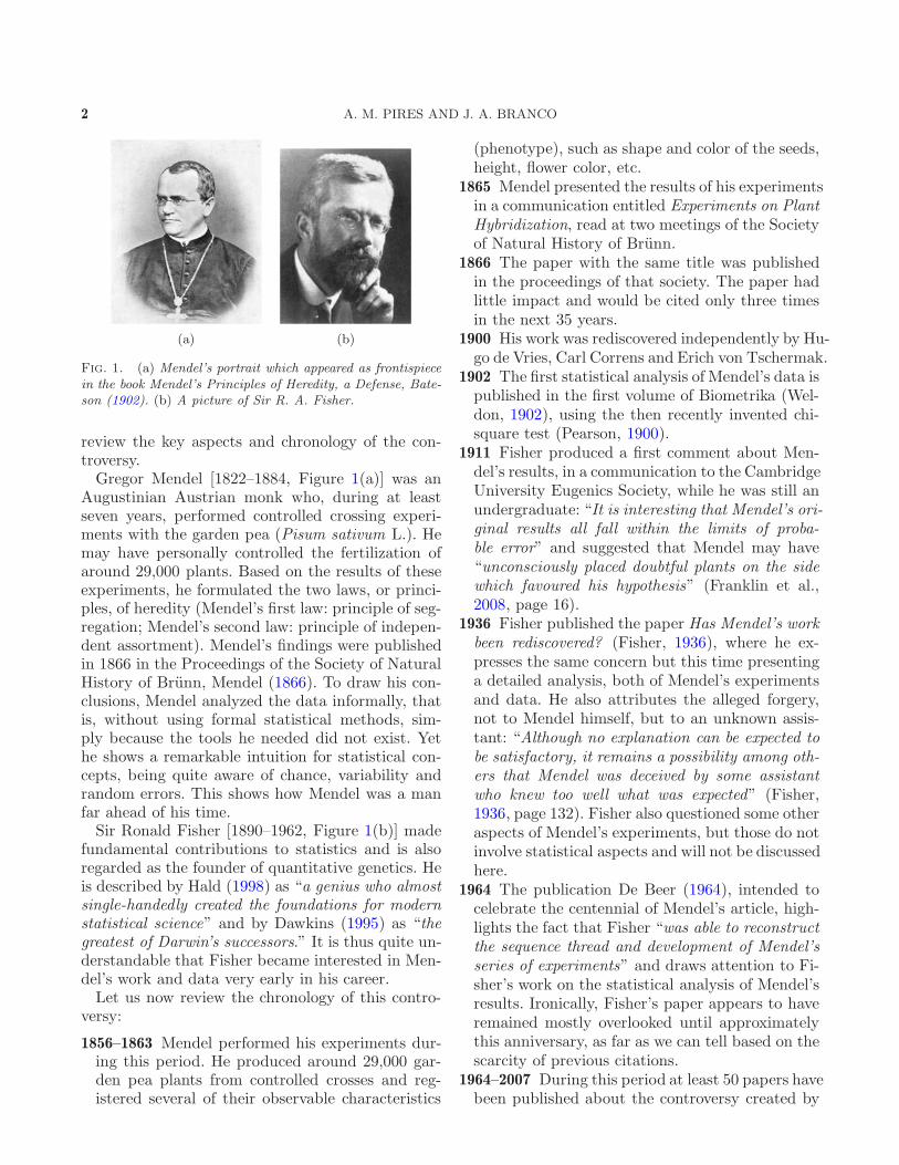
Fig. 1. (a) Mendel’s portrait which appeared as frontispiecein the book Mendel’s Principles of Heredity, a Defense, Bate-son (1902). (b) A picture of Sir R. A. Fisher.

review the key aspects and chronology of the con-troversy.Gregor Mendel [1822–1884, Figure 1(a)] was an

Augustinian Austrian monk who, during at leastseven years, performed controlled crossing experi-ments with the garden pea (Pisum sativum L.). Hemay have personally controlled the fertilization ofaround 29,000 plants. Based on the results of theseexperiments, he formulated the two laws, or princi-ples, of heredity (Mendel’s first law: principle of seg-regation; Mendel’s second law: principle of indepen-dent assortment). Mendel’s findings were publishedin 1866 in the Proceedings of the Society of NaturalHistory of Brunn, Mendel (1866). To draw his con-clusions, Mendel analyzed the data informally, thatis, without using formal statistical methods, sim-ply because the tools he needed did not exist. Yethe shows a remarkable intuition for statistical con-cepts, being quite aware of chance, variability andrandom errors. This shows how Mendel was a manfar ahead of his time.Sir Ronald Fisher [1890–1962, Figure 1(b)] made

fundamental contributions to statistics and is alsoregarded as the founder of quantitative genetics. Heis described by Hald (1998) as “a genius who almostsingle-handedly created the foundations for modernstatistical science” and by Dawkins (1995) as “thegreatest of Darwin’s successors.” It is thus quite un-derstandable that Fisher became interested in Men-del’s work and data very early in his career.Let us now review the chronology of this contro-

versy:

1856–1863 Mendel performed his experiments dur-ing this period. He produced around 29,000 gar-den pea plants from controlled crosses and reg-istered several of their observable characteristics

(phenotype), such as shape and color of the seeds,height, flower color, etc.

1865 Mendel presented the results of his experimentsin a communication entitled Experiments on PlantHybridization, read at two meetings of the Societyof Natural History of Brunn.

1866 The paper with the same title was publishedin the proceedings of that society. The paper hadlittle impact and would be cited only three timesin the next 35 years.

1900 His work was rediscovered independently by Hu-go de Vries, Carl Correns and Erich von Tschermak.

1902 The first statistical analysis of Mendel’s data ispublished in the first volume of Biometrika (Wel-don, 1902), using the then recently invented chi-square test (Pearson, 1900).

1911 Fisher produced a first comment about Men-del’s results, in a communication to the CambridgeUniversity Eugenics Society, while he was still anundergraduate: “It is interesting that Mendel’s ori-ginal results all fall within the limits of proba-ble error” and suggested that Mendel may have“unconsciously placed doubtful plants on the sidewhich favoured his hypothesis” (Franklin et al.,2008, page 16).

1936 Fisher published the paper Has Mendel’s workbeen rediscovered? (Fisher, 1936), where he ex-presses the same concern but this time presentinga detailed analysis, both of Mendel’s experimentsand data. He also attributes the alleged forgery,not to Mendel himself, but to an unknown assis-tant: “Although no explanation can be expected tobe satisfactory, it remains a possibility among oth-ers that Mendel was deceived by some assistantwho knew too well what was expected” (Fisher,1936, page 132). Fisher also questioned some otheraspects of Mendel’s experiments, but those do notinvolve statistical aspects and will not be discussedhere.

1964 The publication De Beer (1964), intended tocelebrate the centennial of Mendel’s article, high-lights the fact that Fisher “was able to reconstructthe sequence thread and development of Mendel’sseries of experiments” and draws attention to Fi-sher’s work on the statistical analysis of Mendel’sresults. Ironically, Fisher’s paper appears to haveremained mostly overlooked until approximatelythis anniversary, as far as we can tell based on thescarcity of previous citations.

1964–2007 During this period at least 50 papers havebeen published about the controversy created by

EXPLAINING THE MENDEL–FISHER CONTROVERSY 3

Fisher. Some elucidative titles: The too-good-to-be-true paradox and Gregor Mendel (Pilgrim, 1984);Are Mendel’s results really too close? (Edwards,1986a); Mud Sticks: On the Alleged Falsificationof Mendel’s Data (Hartl and Fairbanks, 2007).

2008 A group of scientists from different fields,Franklin (Physics and History of Science), Ed-wards (Biometry and Statistics, and curiously, Fi-sher’s last student), Fairbanks (Plant and WildlifeSciences), Hartl (Biology and Genetics) and Sei-denfeld (Philosophy and Statistics), who have pre-viously published work on the controversy, mergedtheir most relevant papers and published the bookEnding the Mendel–Fisher Controversy. But is itreally the end of the controversy? The authors dis-miss all of the issues raised by Fisher except the“too good to be true” (pages 68 and 310).In a very interesting book review, entitled CSI:Mendel, Stigler (2008) adds: “. . . an actual end tothat discussion is unlikely to be a consequence ofthis book.” and “. . . thanks to these lucid, insight-ful and balanced articles, another generation willbe able to join the quest with even better under-standing.”

3. EXPERIMENTS AND DATA

Before introducing the data and discussing thecorresponding statistical analysis, it is important tounderstand the experiments and the scientific hy-potheses under evaluation. Using a classification sim-ilar to that used by Fisher, the experiments can beclassified as follows: single trait, bifactorial, trifac-torial and gametic ratios experiments.Single trait experiments. These concern the trans-

mission of only one binary characteristic (or trait) ata time. Mendel examined seven traits, two observ-able in the seeds (seed shape: round or wrinkled;seed color: yellow or green) and five in the plants(flower color: purple or white; pod shape: inflated orconstricted; pod color: yellow or green; flower posi-tion: axial or terminal; stem length: long or short).First Mendel obtained what are now called “purelines,” with each of the two forms of the seven char-acters, that is, plants which yielded perfectly con-stant and similar offspring. When crossing the twopure lines, F0, for each character Mendel observedthat all the progeny, F1, presented only one of theforms of the trait. He called this one the dominantform and represented it by A. The other form wascalled recessive and denoted by a. In the seven traits

Fig. 2. A schematic representation of Mendel’s single traitexperiments (in modern notation and terminology).

listed above the first form is the dominant and thesecond is the recessive. He then crossed the F1 indi-viduals (which he called the hybrids) and observedthat in the resulting generation, F2, there were indi-viduals of the two original types, approximately inthe ratio 3 : 1 of the dominant type to the recessivetype. In modern notation and terminology, we arestudying a phenotype with possible values “A” and“a” governed by a single gene with two alleles (Aand a, where the first is dominant). The F0 plantsare homozygous AA (genotype AA, phenotype “A”)or aa (genotype aa, phenotype “a”), the F1 are allheterozygous Aa (genotype Aa, phenotype “A”),the F2 plants can have genotype AA (phenotype“A”), genotype Aa (phenotype “A”) and genotypeaa (phenotype “a”). When Mendel self-fertilized theF2 plants with phenotype “A,” he found that aboutone-third of these always produced phenotype “A”progeny, while about two-thirds produced pheno-type “A” and phenotype “a” progeny in the ratio3 : 1. This process is schematically represented inFigure 2, where (F3) refers to the progeny of theself-fertilized F2 individuals.Table 1 presents the data given in Mendel (1866)

for the single trait experiments just described. As anillustration of the variability of the results betweenplants, Mendel also presented the individual figuresobtained for the ten first plants of each of the ex-periments relative to the seed characteristics (theseare referred to by Fisher as “illustrations of plantvariation,” cf. Table 5).Bifactorial experiment. This is an experiment sim-

ilar to the single trait experiments but observingtwo characteristics simultaneously (seed shape, A,and seed color, B, starting from pure lines on both).The aim was to observe how the two traits are com-bined. Mendel postulated and confirmed from theresults of the experiment that the traits considered


Table 1

Data given in Mendel (1866) for the single trait experiments. “A” (“a”) denotes the dominant (recessive) phenotype; A (a)denotes the dominant (recessive) allele; n is the total number of observations per experiment (that is, seeds for the seed trait

experiments and plants otherwise); n“A”, n“a”, nAa and nAA denote observed frequencies

Obs. freq. Theor. ratioTrait “A” “a” n n“A” n“a” “A” : “a”

Seed shape round wrinkled 7324 5474 1850 3 : 1Seed color yellow green 8023 6022 2001 3 : 1Flower color purple white 929 705 224 3 : 1

F2 Pod shape inflated constricted 1181 882 299 3 : 1Pod color yellow green 580 428 152 3 : 1Flower position axial terminal 858 651 207 3 : 1Stem length long short 1064 787 277 3 : 1

Trait A a n nAa nAA Aa :AA

Seed shape round wrinkled 565 372 193 2 : 1Seed color yellow green 519 353 166 2 : 1Flower color purple white 100 64 36 2 : 1

(F3) Pod shape inflated constricted 100 71 29 2 : 1Pod color yellow green 100 60 40 2 : 1Flower position axial terminal 100 67 33 2 : 1Stem length long short 100 72 28 2 : 1Pod color (rep.) yellow green 100 65 35 2 : 1

Table 2

Data from the bifactorial experiment [as organized by Fisher(1936)]

AA Aa aa Total

BB 38 60 28 126Bb 65 138 68 271bb 35 67 30 132

Total 138 265 126 529

are assorted independently.1 That is, given a traitA with an F2 generation AA, Aa and aa in theratio 1 : 2 : 1, and a trait B with BB, Bb and bbin the same ratio, combining the two independentlyleads to the genotypes and theoretical ratios repre-sented in Figure 3. The data, organized by Fisherfrom Mendel’s description, are shown in Table 2.Trifactorial experiment. This experiment is also

similar to the previous experiment but consideringthe crossing of three traits (seed shape, seed colorand flower color). The data, organized by Fisherfrom Mendel’s description, are shown in Table 3,

1This independence hypothesis is also a matter of contro-versy (did Mendel detect linkage?) and has been discussedthoroughly in the literature (see Franklin et al., 2008, pages288–292).

Fig. 3. Genotypes and theoretical ratios for the bifactorialexperiment.

Fig. 4. Theoretical ratios for the trifactorial experiment.

whereas the corresponding theoretical ratios are gi-ven in Figure 4.Gametic ratios experiments. In this last series of

experiments Mendel designed more elaborated crossesin order to obtain “conclusions as regards the com-position of the egg and pollen cells of hybrids.” Thecrosses are represented in Figure 5 and the data areshown in Table 4.We will also use an organization of the data into 84

binomial experiments, similar to the one proposedby Edwards (1986a, see also Franklin et al., 2008,Chapter 4). The data set used is described in detailin Appendix A.


Table 3

Data from the trifactorial experiment [as organized by Fisher (1936)]

CC Cc cc TotalAA Aa aa Total AA Aa aa Total AA Aa aa Total AA Aa aa Total

BB 8 14 8 30 22 38 25 85 14 18 10 42 44 70 43 157Bb 15 49 19 83 45 78 36 159 18 48 24 90 78 175 79 332bb 9 20 10 39 17 40 20 77 11 16 7 34 37 76 37 150

Total 32 83 37 152 84 156 81 321 43 82 41 166 159 321 159 639

Table 4

Data from the gametic ratios experiments (Mendel,1866)

Exp. nObservedfrequencies

Theoreticalratio

TraitsA B

1 90 20 23 25 22 1 : 1 : 1 : 1 seed shape seed color2 110 31 26 27 26 1 : 1 : 1 : 1 seed shape seed color3 87 25 19 22 21 1 : 1 : 1 : 1 seed shape seed color4 98 24 25 22 27 1 : 1 : 1 : 1 seed shape seed color5 166 47 40 38 41 1 : 1 : 1 : 1 flower color stem length

All the computations and Monte Carlo simula-tions described were carried out using the R software(R Development Core Team, 2008). The full code isavailable upon request.

4. STATISTICAL ANALYSIS: INCRIMINATING

EVIDENCE

4.1 Fisher’s Analysis

As mentioned in Section 2, Fisher (1936) presentsa very detailed analysis of both Mendel’s experi-ments and data. Here we will concentrate on a par-ticular part of the analysis, the chi-square analysissummarized in Table V, page 131, of Fisher (1936),which is reproduced in Table 5. This table has beenthe subject of a lot of debate, and it constitutes themain evidence for the “too good to be true” aspect ofMendel’s data as claimed by Fisher. We later presenta new explanation for this evidence.The analysis is very simple to describe: for each

separate experiment, Fisher performed a chi-squaregoodness-of-fit test, where H0 specifies the probabil-ities implied by the theoretical ratios. Note that, forthe two category cases, this is equivalent to the usualasymptotic test for a single proportion. Then he ag-gregated all the tests by summing the chi-squarestatistics as well as the associated number of degreesof freedom and computed an aggregated p-value of

Table 5

Fisher’s chi-square analysis (“Deviations expected andobserved in all experiments”)

Experiments Expectation χ2

Probabilityof exceedingdeviationsobserved

3 : 1 ratios 7 2.1389 0.952 : 1 ratios 8 5.1733 0.74Bifactorial 8 2.8110 0.94Gametic ratios 15 3.6730 0.9987Trifactorial 26 15.3224 0.95

Total 64 29.1186 0.99987Illustrations of

plant variation 20 12.4870 0.90

Total 84 41.6056 0.99993

0.99993. This would mean that if Mendel’s exper-iments were repeated, under ideal conditions suchthat all the null-hypotheses are true, and all theBernoulli trials—within and between experiments—are independent, the probability of getting an overallbetter result would be 7/100,000.Fisher’s chi-square results were recomputed just

to confirm that we are working with exactly thesame data and assumptions. The results, given inthe first 4 columns of Table 6, show that the statis-tics (χ2

obs) are identical to Fisher’s values, but thereare some differences in the p-values which certainlyreflect different methods of computing the chi-squaredistribution function [p-value (χ2

df) denotes the p-valuecomputed from a χ2 distribution with df degrees offreedom, that is, P (χ2

df > χ2obs)].

The table also gives the Monte Carlo (MC) esti-mates of the p-values (and corresponding standarderrors, se) based on 1,000,000 random repetitions ofthe experiments using binomial or multinomial sam-pling, whichever is appropriate, as considered by Fi-sher. A more detailed description of the Monte Carlosimulation is given in Appendix B.1.


Comparing the list of χ2df p-values with the list of

MC p-values, the conclusion is that the approxima-tion of the sampling distribution of the test statis-tic by the chi-square distribution is very accurate,and that Fisher’s analysis is very solid [our resultsare also in accordance with the results of similarbut less extensive simulations described in Novitski(1995)]. Moreover, we can also conclude that the evi-dence “against” Mendel is greater than that given byFisher, since an estimate of the probability of gettingan overall better result is now 2/100,000. We havealso repeated the chi-square analysis considering the84 binomial experiments (results given in the next3 columns of Table 6) and concluded that the twosampling models are almost equivalent, the secondone (only binomial) being slightly more favorableto Fisher and less favorable to Mendel. Acting inMendel’s defense, the results will be more convinc-ing if we prove our case under the least favorablescenario. Thus, for the remaining investigation, weuse only the binomial model and data set.Franklin et al. (2008, pages 29–67) provide a com-

prehensive systematic review of all the papers pub-lished since the 1960s in reaction to Fisher’s ac-cusations. The vast majority of those authors tryto put forward arguments in Mendel’s defense. Weonly highlight here some of the more relevant con-tributions regarding specifically the “too good to betrue” conclusion obtained from the chi-square anal-ysis. The majority of the reactions/arguments canbe generically classified into three categories.In the first category we consider those who do not

believe in Fisher’s analysis. This is the case of Pil-

grim (1984, 1986) who in the first paper affirms tohave detected “four paradoxical elements in Fisher’sreasoning” and who, in the second, claims to havebeen able to show where Fisher went wrong. Pil-grim’s arguments are related to the application ofthe chi-square global statistic and were refuted byEdwards (1986b).As a second category, those who, in spite of believ-

ing that Fisher’s analysis is correct, think it is toodemanding and propose alternative ways to analyzeMendel’s data. Edwards (1986a) analyzes the distri-bution of a set of test statistics, whereas Seidenfeld(1998) analyzes the distribution of a set of p-values.They both find the “too good to be true” charac-teristic and come to the conclusion that Mendel’sresults were adjusted rather than censored.2 Themethods of Leonard (1977) and Robertson (1978),who analyzed only a small part of the data, couldalso be classified here, but, according to Piegorsch(1983), their contribution to advance the debate wasmarginal.Finally, as a third category, those who believe

Fisher’s analysis is correct under its assumptions(binomial/multinomial sampling, independent exper-iments) and then try to find a reason or explanation,other than deliberate cheating, for the observationof a very high global p-value. Such an explanation

2These are the precise words used in the cited references(Edwards, 1986b and Seidenfeld, 1998). They mean that someresults have been slightly modified to fit Mendel’s expecta-tions (“adjusted”), instead of just being eliminated (“cen-sored” or “truncated”).

(a)

(b)

Fig. 5. Schematic representation of the gametic ratios experiments: (a) experiments 1–4 in Table 4; (b) experiment 5 inTable 4.

EXPLAIN

ING

THE

MENDEL–FISHER

CONTROVERSY

7

Table 6

Results of the chi-square analysis considering different models and methods for computing/estimating p-values. Each line corresponds to a different type ofexperiment in Mendel’s paper: single trait, 3 : 1 ratios; single trait, 2 : 1 ratios; bifactorial (BF); gametic ratios (GR); trifactorial (TF); and illustrations of plant

variation (PV). df : degrees of freedom of the asymptotic distribution of the χ2 test statistic under H0 (Mendel’s theory); χ2obs: observed value of the χ2 test

statistic; p-value (χ2df): p-value computed assuming that the test statistic follows, under H0, a χ2 distribution with df degrees of freedom; p-value (MC): p-value

estimated from Monte Carlo simulation. se: standard error of the p-value (MC) estimate

Fisher(binomial + multinomial)

Model A Model BEdwards (binomial) α= 0.094 α= 0.201 α= 0.362 β = 0.261 β = 0.455 β = 0.634

p-value p-value p-value p-value p-value p-value p-value p-value p-value p-valueExp. df χ2

obs(χ2

df) (MC) χ2

obs(χ2

df) (MC) (MC) (MC) (MC) (MC) (MC) (MC)

(se) (se) (se) (se) (se) (se) (se) (se)

3:1 7 2.1389 0.9518 0.9519 2.1389 0.9518 0.9517 0.9069 0.8286 0.6579 0.9023 0.8446 0.7701(0.0002) (0.0002) (0.0003) (0.0004) (0.0005) (0.0003) (0.0004) (0.0004)

2:1 8 5.1733 0.7389 0.7401 5.1733 0.7389 0.7393 0.4955 0.2374 0.1156 0.6044 0.4826 0.3586(0.0004) (0.0004) (0.0005) (0.0004) (0.0003) (0.0005) (0.0005) (0.0005)

BF 8 2.8110 0.9457 0.9462 2.7778 0.9475 0.9482 0.8838 0.7839 0.5926 0.8914 0.8248 0.7376(0.0002) (0.0002) (0.0003) (0.0004) (0.0005) (0.0003) (0.0004) (0.0004)

GR 15 3.6730 0.9986 0.9987 3.6277 0.9987 0.9987 0.9950 0.9811 0.9063 0.9939 0.9827 0.9584(0.00004) (0.00004) (0.00007) (0.0001) (0.0003) (0.00008) (0.0001) (0.0002)

TF 26 15.3224 0.9511 0.9512 15.1329 0.9549 0.9555 0.6973 0.2917 0.0812 0.8493 0.6941 0.4847(0.0002) (0.0002) (0.0004) (0.0005) (0.0003) (0.0004) (0.0005) (0.0005)

Tot. 64 29.1185 0.99995 0.99995 28.8506 0.99995 0.99995 0.9917 0.8175 0.2965 0.9980 0.9800 0.8887(0.000007) (0.000007) (0.00008) (0.0004) (0.0005) (0.00004) (0.0001) (0.0003)

PV 20 12.4870 0.8983 0.9000 12.4870 0.8983 0.9003 0.5932 0.2196 0.0684 0.7582 0.5922 0.4028(0.0003) (0.0003) (0.0005) (0.0004) (0.0003) (0.0004) (0.0005) (0.0005)

Tot. 84 41.6055 0.99997 0.99998 41.3376 0.99998 0.99998 0.9860 0.6577 0.1176 0.9980 0.9733 0.8348(0.000005) (0.000005) (0.0001) (0.0005) (0.0003) (0.00004) (0.0002) (0.0004)


has to imply the failure of at least one of those twoassumptions. Moreover, that failure has to occur ina specific direction, the one which would reduce thechi-square statistics: for instance, the distributionof the phenotypes is not binomial and has a smallervariance than the binomial. The various explana-tions that have been put forward can be dividedinto the following: biological, statistical and metho-dological.Among the biological candidate explanations, one

that received some attention was the “Tetrad PollenModel” (see Fairbanks and Schaalje, 2007).Few purely statistical explanations have been pro-

posed and most of them are anecdotal. One thatraised some discussions was a proposal of Weiling(1986) who considers, based on the tetrad pollenmodel just mentioned, a distribution with smallervariance than the binomial for some of the experi-ments, and hypergeometric for other experiments.The majority of the suggested explanations are

of a methodological nature: the “anonymous” assis-tant (Fisher); sequential procedures, like stoppingthe count when the results look good (several au-thors); discard plants or complete experiments dueto suspicions of some experimental error, like pollencontamination (Dobzhansky, 1967); luck(?); inher-ent difficulties in the classification of the pheno-types (Root-Bernstein, 1983); data selection for pre-sentation (Di Trocchio, 1991; Fairbanks and Ryt-ting, 2001).It is important to keep in mind that for an expla-

nation to be acceptable as the solution to the con-troversy it must fulfill a number of conditions: (i)it must be biologically plausible and/or experimen-tally verifiable; (ii) it must be statistically correctand pass the chi-square and eventually other statis-tical analyses aiming at disentangling the enigma;and (iii) assuming that Mendel’s theory is correctand that he is not guilty of any deliberate fraud,it has to find support in and it can not contradictMendel’s writings. The fact is that all the explana-tions which were proposed up to now failed in oneor other of these requirements.In summary, Fisher’s analysis has resisted all at-

tempts to be either refuted or explained. Our sim-ulation also confirms that, under the standard as-sumptions, Fisher’s tests and conclusions are cor-rect.

4.2 Analysis of p-Values

As mentioned in Section 3, Edwards (1986a) pro-posed an organization of the data into 84 binomial

experiments. He then used the data to compute whathe called (signed) χ values, that is, the square rootof the chi-square statistic with the sign of the devi-ation (“+” if observed > expected and “−” if ob-served < expected). Since all the tests have one de-gree of freedom and, assuming that Mendel’s theoryis correct, the χ values should follow approximatelya standard normal distribution. However, a normalqqplot of those values shows apparently a large de-viation from normality (Franklin et al., 2008, Fig-ures 1.1 and 1.2, page 49). From the shape of theplot Edwards (1986a) concluded that it appears tobe more likely that Mendel’s results were adjustedrather than truncated. This conclusion, to whichSeidenfeld (1998) also arrives, and later Franklin etal. (2008) agree, would render some of the most plau-sible methodological explanations not viable.Another approach is to analyze the p-values of the

individual χ21 tests. This idea was explored by Sei-

denfeld (1998); (see also Franklin et al., 2008, Fig-ures 1.3 and 1.4, page 59), although not so system-atically as in the analysis provided here. The 84 χvalues, along with the 84 p-values, are also given inAppendix A.As for Fisher’s and Edwards’ analysis, we know

what to expect under the ideal assumptions. Thatis, if: (i) Mendel’s theory is valid for all the experi-ments, or, equivalently, if the null hypotheses of thechi-square tests are true in all cases; (ii) the ex-periments were performed independently and as de-scribed in Mendel’s paper; and (iii) the chi-squareapproximation is valid, then the p-values follow auniform (0,1) distribution. Therefore, the plot of theempirical cumulative distribution function (e.c.d.f.)3

of the p-values should be close to the diagonal of the(0,1) × (0,1) square. However, the e.c.d.f., plottedin Figure 6, reveals a marked difference from uni-formity. This visual assertion was confirmed by aKolmogorov–Smirnov (K–S) goodness-of-fit test (p-value = 0.0036, details in Appendix B.2). We cantherefore conclude with a high confidence that thedistribution of the p-values deviates from a uniform(0,1) distribution. It is then natural to wonder aboutthe kind of deviation and its meaning. In Figure 6we also plot the cumulative distribution function(c.d.f.) of the maximum of two uniform (0,1) ran-dom variables, y = x2, since this is central to theexplanation that we give later for Mendel’s results.

3The e.c.d.f. is defined, for a random sample of size n, asFn(x) = {n. of observations≤ x}/n.


Fig. 6. Empirical cumulative distribution function of thep-values (stair steps line); cumulative distribution function ofthe uniform (0,1) random variable (straight line); cumulativedistribution function of the maximum of two (0,1) uniformrandom variables (curve).

Fig. 7. Histogram of the 84 p-values observed [the dashedline indicates the expected frequencies under the uniform (0,1)distribution].

The histogram of the p-values (Figure 7) is help-ful for our argumentation. One could perhaps thinkthat the uniform distribution is not a good fit forthe sample of p-values because some of the null hy-potheses are not true. But if that were the case, wewould observe an excess of values close to 0, andthe histogram shows precisely the opposite. Possi-ble reasons for this to happen are as follows: eitherthe data shows that the hypotheses are “more true,”that is, the data are better than expected under thenull hypotheses, or there is something wrong withthe assumptions (and possible explanations are, asfor the chi-square analysis, smaller variance than bi-nomial, or lack of independence).

In conclusion, the p-value analysis shows that theprobability of obtaining overall results as good orbetter than those obtained by Mendel (under theassumptions) is about 4/1000. This “evidence” isnot as extreme as the 2/100,000 resulting from thechi-square analysis but points in the same direction.

5. A PLAUSIBLE EXPLANATION

5.1 A Statistical Model for the p-Values

In the previous section we have shown that thereis strong evidence that the p-values are not uni-formly distributed. What is then their distribution,and how can it be explained?The shape of the e.c.d.f. provides a hint: it re-

sembles the function x2, which is the c.d.f. of themaximum of two uniform (0,1) random variables,as can easily be shown. It appears that some c.d.f.intermediate between that corresponding to a uni-form (0,1) random variable and that correspondingto the maximum of two uniform (0,1) random vari-ables best fits the e.c.d.f. of the sample p-values (seeFigure 6).One explanation for this is the following: suppose

Mendel has repeated some experiments, presumablythose which deviate most from his theory, and re-ports only the best of the two. A related possibil-ity was suggested by Fairbanks and Rytting (2001,page 743): “We believe that the most likely explana-tion of the bias in Mendel’s data is also the simplest.If Mendel selected for presentation a subset of his ex-periments that best represented his theories, χ2 anal-ysis of those experiments should display a bias.” Theauthors support this explanation with citations fromMendel’s work. We have found only an attempt toverify the effect of such a selection procedure on thechi-square analysis (footnote number 62, page 73, ofFranklin et al., 2008), but it seems to lead to thewrong conclusion, as we conclude later that the ef-fect of the given explanation on the chi-square anal-ysis is very small. Moreover, the explanation appearsto have been abandoned because “It does not [how-ever] address the demonstration, by both Edwardsand Seidenfeld, that Mendel’s data had not merelybeen truncated, but adjusted” (Franklin et al., 2008,page 62).Both procedures described in the previous para-

graph for selecting the data to be presented canbe modeled by assuming that an experiment is re-peated whenever its p-value is smaller than α, where0≤ α≤ 1 is a parameter fixed by the experimenter,


and then only the one with the largest p-value isreported.4 Under this selection model (from now onnamed “model A”), the c.d.f. of the p-values of theexperiments reported is given by

Fα(x) =

{

x2, if 0≤ x≤ α,(1 + α)x− α, if α< x≤ 1.

(5.1)

Proof. For a given experiment, denote by Xthe p-value effectively reported. We have that X =X1, ifX1 ≥ α andX =max(X1,X2) ifX1 < α, whereX1 and X2 represent the p-values obtained in thefirst and the second realization of the experiment (ifthere is one), respectively. Assume that X1 and X2

are independent and identically distributed continu-ous uniform (0,1) random variables (i.e., the two re-alizations of the experiment are independent and theassociated null hypothesis is true), that is, P (X1 ≤x) = P (X2 ≤ x) = x, 0≤ x≤ 1. In the derivation ofFα(x) = P (X ≤ x), the cases 0≤ x < α and α≤ x≤1 are considered separately.If 0≤ x < α,

P (X ≤ x) = P (max(X1,X2)≤ x)

= P ({X1 ≤ x} ∩ {X2 ≤ x})= P (X1 ≤ x)P (X2 ≤ x) = x2.

If α≤ x≤ 1,

P (X ≤ x)

= P (({X ≤ x} ∩ {X1 <α})∪ ({X ≤ x} ∩ {X1 ≥ α}))

= P ({X ≤ x} ∩ {X1 < α})+P ({X ≤ x} ∩ {X1 ≥ α})

= P ({max(X1,X2)≤ x} ∩ {X1 < α})+P ({X1 ≤ x} ∩ {X1 ≥ α})

= P ({X1 < α} ∩ {X2 ≤ x}) + P (α≤X1 ≤ x)

= x×α+ (x− α). �

Suppose that model A holds but α is unknown andmust be estimated using the available sample of 84binomial p-values. The minimum distance estimatorbased on the Kolmogorov distance, also called the“Minimum Kolmogorov–Smirnov test statistic esti-mator” (Easterling, 1976), provides one method for

4Note that this is just an idealized model on which to baseour explanation. We are not suggesting that Mendel actuallycomputed p-values!

estimating α. This estimate is the value of α whichminimizes the K–S statistic,

D(α) = supx

|Fn(x)−Fα(x)|(5.2)

for testing the null hypothesis that the c.d.f. of thep-values is Fα. Equivalently, the estimate can be de-termined by finding the value of α which maximizesthe p-value of the K–S test, p(α), since p(·) is astrictly decreasing function of D(·).Figure 8 shows the plot of the K–S p-values, p(α),

as a function of α, together with the point esti-mate, α = 0.201 (D = 0.0623, P = 0.8804), and a

Fig. 8. Plot of the p-value of the K–S test as a functionof the parameter, showing the point estimate and the 90%confidence interval, for model A.

Fig. 9. Empirical cumulative distribution function of thep-values and fitted model (solid line: α= 0.201; dashed lines:90% confidence limits).


Fig. 10. Plot of the p-value of the K–S test as a functionof the parameter, showing the point estimate and the 90%confidence interval, for model B.

90% confidence interval for α, (0.094; 0.362). A de-tailed explanation on how these figures were ob-tained is given in Appendix B.3. Figure 9 confirmsthe good model fit.This model can also be submitted to Fisher’s chi-

square analysis. Assuming it holds for a certain valueα0, we may still compute “chi-square statistics,” butthe p-values can no longer be obtained from the chi-square distribution. However, they can be accuratelyestimated by Monte Carlo simulation. The differ-ence to the previous simulations is that statisticsand (χ2

1) p-values were always computed (for eachof the 84 binomial cases and each random repeti-tion) and whenever that p-value was smaller thanα0 another binomial result was generated and thestatistic recorded was the minimum of the two.The simulation results obtained for three values

of α (point estimate and limits of the confidenceinterval) are presented in the three columns of Ta-ble 6 under the heading “Model A.” The p-valuesin these columns (and especially those correspond-ing to α= 0.201) do not show any sign of being tooclose to one anymore, in fact, they are perfectly rea-sonable. In Appendix C we present a more detailed(and technical) justification of the results obtained.The conclusion is that our model explains Fisher’s

chi-square results: Mendel’s data are “too good tobe true” according to the assumption that all thedata presented in Mendel’s paper correspond to allthe experiments Mendel performed, or to a randomselection from all the experiments. When this as-sumption is replaced by model A the results can no

longer be considered too good. So we conclude thatmodel A is a reasonable statistical explanation forthe controversy. We do not pretend that it is neces-sarily the “true” model; however, it is very simpleand does provide extra insight into the complexity ofthis historical debate and in this sense it is useful.As G.E.P. Box said, “All models are wrong, somemodels are useful.”We have just seen how the suggested selection

mechanism can make Mendel’s results (which weknow are in fact correct) look too correct. This raisesa related question of general interest to all experi-mental sciences: is it possible to make an incorrecttheory look correct by applying this or a similar se-lection mechanism? Although a detailed answer tothis question is beyond the scope of this paper, inAppendix D we give an idea on how a generalizationof model A can be used to explore the question.

5.2 Alternative Models

No doubt there are many models, perhaps morecomplicated than ours, that explain Mendel’s dataas well as, or perhaps better than, ours. A relevantquestion to ask, then, is whether any model similarto ours, more specifically, a one parameter modelwith c.d.f. varying between x and x2, would producesimilar results and also a reasonable interpretation.To show that the answer to this question is nega-

tive, we have considered an alternative model, modelB, with distribution function computed as a lin-ear combination of the “extreme” models, that is,with c.d.f. given by Fβ(x) = (1 − β) × x + β × x2,with 0≤ β ≤ 1. This is mathematically simpler thanmodel A and its interpretation in terms of the de-sign of the experiments could be: Mendel would alsodecide to repeat some experiments and report onlythe best result of both (the original and the rep-etition), but the decision to repeat would be takenrandomly with probability β, for instance, by throw-ing a fair coin (β = 0.5) or something similar. Ap-plying the methods described in Appendix B.3 tothis model, we obtain (see Figure 10) β = 0.45 (K–S test: D = 0.0875, P = 0.5131) and CI 90%(β) =(0.261; 0.634). Figure 11 shows the e.c.d.f. of the p-values and the c.d.f. of model B with β = 0.45 (solidline) and β = 0.261,0.634 (dashed lines). Comparedto Figure 9, the fit of model B looks worse than thefit of model A, but it could still be considered ac-ceptable. However, in what concerns the chi-squareanalysis, model B is unable to produce good results


Fig. 11. E.c.d.f. of the p-values and alternative model (solidline: β = 0.45; dashed lines: 90% confidence limits).

(cf. the last three columns in Table 6). The aggre-gated p-value (84 df ) still points to “too good to betrue” except maybe for the last column, which cor-responds to the odd situation of randomly repeatingabout 60% of the experiments! We have presentedmodel B as just an exercise to show a specific point,it does not correspond to a plausible procedure asdoes model A.

5.3 Further Support for the Proposed Model

As a harder challenge, we observed the behaviorof each of the models in the context of Edwards’chi values analysis, mentioned at the beginning ofSection 4.2. The results of a simple simulation exer-cise are represented in the four plots in Figure 12.All the plots are normal quantile–quantile plots, andcontain the representation of the actual sample of 84χ values (thick line). Each plot also represents 100samples of simulated 84 χ values, generated by thecorresponding model (gray thin lines), plus a “syn-thetic” sample obtained by averaging the orderedobservations of those 100 simulated samples (inter-mediate line). Plot (a): the samples were generatedfrom a standard normal random variable (i.e., fromthe asymptotic distribution of the χ values underthe ideal assumptions, binomial sampling and in-dependent experiments). Plot (b): in this case theχ values were obtained (by transformation of theχ2 values) from the first 100 samples used to ob-tain the results given in the columns with heading“Edwards” in Table 6. Plot (c): similar to the pre-vious but with the samples generated under modelA. Plot (d): idem with model B.

From the top plots we conclude that the Normaland the Binomial models are very similar and donot explain the observed values, whereas from thebottom plots we can see that model A provides amuch better explanation of the χ values observedthan model B. These conclusions are no longer sur-prising, in the face of the previous evidence; how-ever, we shall remark that the several analyses arenot exactly equivalent, so the previous conclusionswould not necessarily imply this last one.Besides the statistical evidence, which by itself

may look speculative, the proposed model is sup-ported by Mendel’s own words. The following quo-tations from Mendel’s paper (Mendel, 1866, pagenumbers from Franklin et al., 2008) are all relevantto our interpretation:

“it appears to be necessary that all mem-bers of the series developed in each succes-sive generation should be, without excep-tion, subjected to observation” (page 80).

From this sentence we conclude that Mendel wasaware of the potential bias due to incomplete ob-servation, thus, it does not seem reasonable that hewould have deliberately censored the data or usedsequential sampling as suggested by some authors:

“As extremes in the distribution of the twoseed characters in one plant, there wereobserved in Expt. 1 an instance of 43 roundand only 2 angular, and another of 14 roundand 15 angular seeds. In Expt. 2 there wasa case of 32 yellow and only 1 green seed,but also one of 20 yellow and 19 green”(page 86).

“Experiment 5, which shows the greatestdeparture, was repeated, and then in lieuof the ratio of 60 : 40, that of 65 : 35 re-sulted” (page 89).

Here he mentions repetition of an experiment butgives both results (note that he decided to repeat anexperiment with p-value = 0.157). However, later hementions several further experiments (pages 94, 95,99, 100, 113) but presents results in only one case(page 99) and in another suggests that the resultswere not good (page 95):

“In addition, further experiments were madewith a smaller number of experimental plantsin which the remaining characters by twosand threes were united as hybrids: all yieldedapproximately the same results” (page 94).


Fig. 12. Each part of the figure contains a normal quantile–quantile plot of the original 84 Edwards’ χ values (solid thickline), and of 100 samples of simulated 84 χ values from each model (gray thin lines) as well as an intermediate line, locatedin the “middle” of the gray lines, corresponding to a “synthetic” sample obtained by averaging the ordered observations of the100 simulated samples.

“An experiment with peduncles of differ-ent lengths gave on the whole a fairly sat-isfactory results, although the differentia-tion and serial arrangement of the formscould not be effected with that certaintywhich is indispensable for correct exper-iment” (page 95).

“In a further experiment the characters offlower-color and length of stem were ex-perimented upon. . . ” in this case resultsare given, and then concludes “The the-ory adduced is therefore satisfactorily con-firmed in this experiment also” (pages 99/100).

“For the characters of form of pod, colorof pod, and position of flowers, experimentswere also made on a small scale and re-sults obtained in perfect agreement” (page 100).

“Experiments which in this connection werecarried out with two species of Pisum . . .

The two experimental plants differed in 5characters, . . . ” (page 113).

It is likely that the results omitted were worse andthat Mendel may have thought there would be nopoint in showing them anymore (he gave examplesof bad fit to his theory before, page 86).Our model may be seen as an approximation for

the omissions described by Mendel. In conclusion, anunconscious bias may have been behind the wholeprocess of experimentation and if that is accepted,then it explains the paradox and ends the contro-versy at last.

6. CONCLUSION

Gregor Mendel is considered by many a creativegenius and incontestably the founder of genetics.However, as with many revolutionary ideas, his lawsof heredity (Mendel, 1866), a brilliant and impres-sive achievement of the human mind, were not im-mediately recognized, and stayed dormant for about


35 years, until they were rediscovered in 1900. WhenRonald Fisher, famous statistician and geneticist,considered the father of modern statistics, used achi-square test to examine meticulously the datathat Mendel had provided in his classical paper toprove his theory, he concluded that the data wastoo close to what Mendel was expecting, suggest-ing that scientific misconduct had been present inone way or another. This profound conflict raiseda longstanding controversy that has been engagingthe scientific community for almost a century. Sincenone of the proposed explanations of the conflict issatisfactory, a large number of arguments, ideas andopinions of various nature (biological, psychological,philosophical, historical, statistical and others) havebeen continually put forward just like a never endingsaga.This study relies on the particular assumption that

the experimentation leading to the data analyzed byFisher was carried out under a specific unconsciousbias. The argument of unconscious bias has beenconsidered a conceivable justification by various au-thors who have committed themselves to study somevariations of this line of reasoning (Root-Bernstein,1983; Bowler, 1989; Dobzhansky, 1967; Olby, 1984;Meijer, 1983; Rosenthal, 1976; Thagard, 1988; Nis-sani and Hoefler-Nissani, 1992). But all these at-tempts are based on somehow subjective interpreta-tions and throw no definite light on the problem. Onthe contrary, in this paper the type of unconsciousbias is clearly identified and a well-defined statis-tical analysis based on a proper statistical modelis performed. The results show that the model is aplausible statistical explanation for the controversy.The study goes as follows: (i) Fisher results were

confirmed by repeating his analysis on the same realset of data and on simulated data, (ii) inspired byEdwards’ (1986a) approach, we next idealized a con-venient model of a sequence of binomial experimentsand recognized that the p-value produced by thismodel shows a slight increase, although it keeps veryclose to the result obtained by Fisher. This gaveus confidence to work with this advantageous struc-ture, (iii) we focused on the analysis of the p-valuesof the previous model and realized that the p-valuesdo not have a uniform distribution as they should,(iv) the question arose of what the distribution ofthe p-values could be, and we arrived at the sat-isfactory model we propose in the text, (v) finally,assuming that our model holds, and repeating the

chi-square analysis adopted by Fisher, one sees thatthe impressive effect detected by Fisher disappears.Returning to Fisher’s reaction to the paradoxical

situation he encountered, one may think that, de-spite his remarkable investigation (Fisher, 1936) ofMendel’s work, to prove that something had gonewrong with the selection of the experimental data,apparently neither did he question how could thedata have been generated nor did he identify thedefects of the sample or give a statistical explana-tion for the awkward result. In the end Fisher leftan inescapable global impression of scientific mal-practice, a conclusion that he based on a sound sta-tistical analysis.Probity is an essential component of the scientific

work that should always be contemplated to guar-antee credible final results and conclusions. That iswhy all measures should be taken to make sure thatneither conscious nor unconscious bias will affect theresults of the research work. Unfortunately there ex-ists unconscious bias, an intrinsic automatic humandrive based on culture, social prejudice or motiva-tion that is difficult to stop. Hidden bias influencesmany aspects of our decisions, our social behaviourand our work. That is why scientific enterprises in-cluding honourable doctors and well-intentioned pa-tients do not dispense the scientific techniques basedon blind or double blind procedures. In Mendel’scase we all know that there was a profound mo-tivation that could have triggered the bias and inthose days we guess that the attention given to un-conscious bias may have been poor or it may havenot existed at all. Frequently science ends up in de-tecting errors or fraud that have been induced bybias. But there are no errors in Mendel’s laws, orare there? So why are we worried? Anyway, we wishthat Mendel’s unconscious bias coincides with thearrangement we are suggesting in this paper, be-cause if Mendel did what we think he did, the con-troversy is finally over.

APPENDIX A: THE 84 BINOMIAL

EXPERIMENTS

Edwards (1986a) organized Mendel’s data as theresult of 84 binomial experiments. Note that thisinvolves decomposition of the multinomial experi-ments. In this study we have relied on Edwards’ de-compositions. In order to remain as close as possibleto Fisher’s choices, the data from Table 1—alreadybinomial experiments—were included exactly as


shown, unlike Edwards who subtracted the “plant il-lustrations” from these data. According to this pro-cedure, experiment No. 1 (No. 2) is not indepen-dent of the “plant illustrations” Nos 8–17 (Nos 18–27). But, attending to the relative magnitude of thenumber of observations, if we had used Edwards’numbers, the final results would have not been toodifferent and the conclusions would have been thesame. We have also considered the theoretical ratioof 2 : 1 throughout the experiments involving (F3)generations, instead of the ratio 0.63 : 0.37 that Ed-wards used in some cases. The number of binomialexperiments per pair of true probabilities (ratio) isas follows: 42 cases with 0.75 : 0.25 (3 : 1); 15 caseswith 0.5 : 0.5 (1 : 1); 27 cases with 2/3 : 1/3 (2 : 1).Table 7 contains the following information about

the 84 binomial experiments considered in this pa-per:

Trait: binary variable under consideration (the cat-egory of interest is called a “success” and the othercategory is a “failure”) using the following cod-ing: A (seed shape, round or wrinkled), B (seedcolor, yellow or green), C (flower color, purple orwhite), D (pod shape, inflated or constricted), E(pod color, yellow or green), F (flower position,axial or terminal), G (stem length, long or short).The usual notation is used to distinguish pheno-type (italic inside quotation marks) from genotype(italic), and the dominant form (upper case) fromthe recessive (lowercase); see also Section 3 andTable 1.

n: number of observations (Bernoulli trials) of theexperiment.

Observed: observed frequencies of “successes” (n1)and “failures” (n − n1). Under the standard as-sumptions n1 ∼ Bin(n,p), where p is the proba-bility of a “success” in one trial.

p0: theoretical probability of a “success” underMendel’s theory (H0 :p= p0).

χ: observed value of the test statistic to test H0

against H1 :p 6= p0, given by (n1 − np0)/√

np0(1− p0).p-value: p-value of the test. Assuming n is large,p-value = P (χ2

1 > χ2).

APPENDIX B: TECHNICAL DETAILS

B.1 Simulation of the Chi-Square Analysis

In each of the 1,000,000 repetitions a replicateof Mendel’s complete data set was generated, us-ing the probabilities corresponding to the theoret-ical ratios, and multinomial distributions with the

appropriate number of categories (which reduces tothe binomial distribution for the experiments withtwo categories and is strictly multinomial for theremaining, bifactorial, trifactorial and gametic ra-tios). For each replicate, a total “chi-square” statis-tic was computed as Fisher did for the actual dataset. From the 1,000,000 replicates of the test statis-tic it is possible to estimate the p-value of the testwithout knowledge of the sampling distribution ofthe test statistic. Recall that the MC estimate of ap-value (or simulated p-value) associated to a cer-tain observed statistic (which increases as the datadeviate from the null hypothesis) is the number ofrepetitions for which the corresponding simulatedstatistic is larger than the observed statistic (χ2

obs),divided by the number of repetitions. If we denotean MC estimate of a p-value by P , the correspond-ing estimated standard error is se =

√

P (1− P )/B,where B is the number of random repetitions. Thesefigures are also reported in Table 6.

B.2 Analysis of the p-Values

The Kolmogorov–Smirnov (K–S) test is a goodness-of-fit test based on the statistic D = supx |Fn(x)−F0(x)|, where Fn(x) is the e.c.d.f. obtained from arandom sample (x1, . . . , xn) and F0(x) is a hypoth-esized, completely specified, c.d.f. [D is simply thelargest vertical distance between the plots of Fn(x)and F0(x)]. This test was selected for analyzing thec.d.f. of the p-values because it is more powerfulfor detecting deviations from a continuous distribu-tion than other alternatives such as the chi-squaregoodness-of-fit test (Massey, 1951). Under the ap-propriate conditions [F0(x) is continuous, there areno ties in the sample], the exact p-value of the K–Stest can be computed. In our analysis these con-ditions are not exactly met (the true c.d.f. is notcontinuous and because of that there are ties in thedata), so it is necessary to proceed with caution.The first K–S test performed intended to test the

uniformity of the 84 p-values and produced D =0.1913 (P = 0.0036). The “exact” p-value was com-puted after eliminating the ties by addition of asmall amount of noise to each data point (randomnumbers generated from a normal distribution withzero mean and standard deviation 10−7).As there are several approximations involved, we

checked the whole procedure by performing a sim-ulation study similar to the one described in Sec-tion 4.1 for the chi-square analysis. In 1,000,000 ran-dom repetitions of the sample of 84 p-values a simu-lated p-value of 0.0038 (se = 0.00006) was obtained


Table 7

Data from the 84 binomial experiments

Type ofexperiment

ObservedNo. Trait n n1 n− n1 p0 χ p-value

Single trait 1 A 7324 5474 1850 3/4 −0.513 0.608F2 2 B 8023 6022 2001 3/4 0.123 0.903

3 C 929 705 224 3/4 0.625 0.5324 D 1181 882 299 3/4 −0.252 0.8015 E 580 428 152 3/4 −0.671 0.5026 F 858 651 207 3/4 0.591 0.5547 G 1064 787 277 3/4 −0.779 0.436

Illustrations 8 A 57 45 12 3/4 0.688 0.491of plant 9 A 35 27 8 3/4 0.293 0.770variation 10 A 31 24 7 3/4 0.311 0.756F2 11 A 29 19 10 3/4 −1.179 0.238

12 A 43 32 11 3/4 −0.088 0.93013 A 32 26 6 3/4 0.817 0.41414 A 112 88 24 3/4 0.873 0.38315 A 32 22 10 3/4 −0.817 0.41416 A 34 28 6 3/4 0.990 0.32217 A 32 25 7 3/4 0.408 0.68318 B 36 25 11 3/4 −0.770 0.44119 B 39 32 7 3/4 1.017 0.30920 B 19 14 5 3/4 −0.133 0.89521 B 97 70 27 3/4 −0.645 0.51922 B 37 24 13 3/4 −1.424 0.15523 B 26 20 6 3/4 0.227 0.82124 B 45 32 13 3/4 −0.603 0.54725 B 53 44 9 3/4 1.348 0.17826 B 64 50 14 3/4 0.577 0.56427 B 62 44 18 3/4 −0.733 0.463

Bifactorial 28 A 556 423 133 3/4 0.588 0.557experiment 29 B among “A” 423 315 108 3/4 −0.253 0.801F2 30 B among “a” 133 101 32 3/4 0.250 0.802

Trifactorial 31 A 639 480 159 3/4 0.069 0.945experiment 32 B among “A” 480 367 113 3/4 0.738 0.461F2 33 B among “a” 159 122 37 3/4 0.504 0.615

34 C among AaBb 175 127 48 3/4 −0.742 0.45835 C among AaBB 70 52 18 3/4 −0.138 0.89036 C among AABb 78 60 18 3/4 0.392 0.69537 C among AABB 44 30 14 3/4 −1.045 0.29638 C among Aabb 76 60 16 3/4 0.795 0.42739 C among AAbb 37 26 11 3/4 −0.664 0.50640 C among aaBb 79 55 24 3/4 −1.104 0.26941 C among aaBB 43 33 10 3/4 0.264 0.79242 C among aabb 37 30 7 3/4 0.854 0.393

Single trait 43 A 565 372 193 2/3 −0.417 0.677(F3) 44 B 519 353 166 2/3 0.652 0.515

45 C 100 64 36 2/3 −0.566 0.57246 D 100 71 29 2/3 0.919 0.35847 E 100 60 40 2/3 −1.414 0.15748 F 100 67 33 2/3 0.071 0.94449 G 100 72 28 2/3 1.131 0.25850 E 100 65 35 2/3 −0.354 0.724


Table 7

(Continued)

Type ofexperiment

ObservedNo. Trait n n1 n− n1 p0 χ p-value

Bifactorial 51 A among “AB” 301 198 103 2/3 −0.326 0.744experiment 52 A among “Ab” 102 67 35 2/3 −0.210 0.834(F3) 53 B among “aB” 96 68 28 2/3 0.866 0.386

54 B among Aa“B” 198 138 60 2/3 0.905 0.36655 B among AA“B” 103 65 38 2/3 −0.766 0.443

Trifactorial 56 A among “AB” 367 245 122 2/3 0.037 0.971experiment 57 A among “Ab” 113 76 37 2/3 0.133 0.894(F3) 58 B among “aB” 122 79 43 2/3 −0.448 0.654

59 B among Aa“B” 245 175 70 2/3 1.581 0.11460 B among AA“B” 122 78 44 2/3 −0.640 0.52261 C among AaBb 127 78 49 2/3 −1.255 0.21062 C among AaBB 52 38 14 2/3 0.981 0.32763 C among AABb 60 45 15 2/3 1.369 0.17164 C among AABB 30 22 8 2/3 0.775 0.43965 C among Aabb 60 40 20 2/3 0.000 1.00066 C among AAbb 26 17 9 2/3 −0.139 0.89067 C among aaBb 55 36 19 2/3 −0.191 0.84968 C among aaBB 33 25 8 2/3 1.108 0.26869 C among aabb 30 20 10 2/3 0.000 1.000

Gametic 70 A 90 43 47 1/2 −0.422 0.673ratios 71 B among AA 43 20 23 1/2 −0.458 0.647

72 B among Aa 47 25 22 1/2 0.438 0.66273 A 110 57 53 1/2 0.381 0.70374 B among Aa 57 31 26 1/2 0.662 0.50875 B among aa 53 27 26 1/2 0.137 0.89176 A 87 44 43 1/2 0.107 0.91577 B among AA 44 25 19 1/2 0.905 0.36678 B among Aa 43 22 21 1/2 0.153 0.87979 A 98 49 49 1/2 0.000 1.00080 B among Aa 49 24 25 1/2 −0.143 0.88681 B among aa 49 22 27 1/2 −0.714 0.47582 G 166 87 79 1/2 0.621 0.53583 C among Gg 87 47 40 1/2 0.751 0.45384 C among gg 79 38 41 1/2 −0.338 0.736

(the K–S statistic was larger than 0.1903 in 3807repetitions). This is statistically significantly largerthan 0.0036; however, the difference is not mean-ingful from a practical point of view, the “exact”p-value is 3 digits accurate. So we concluded that itis acceptable to use the K–S test as described.There is another aspect which needs to be ana-

lyzed. Because the outcomes of the experiments arebinomial, yielding whole numbers, the actual distri-bution of the p-values is discrete, not uniform con-tinuous. Therefore, we decided to investigate the dif-ferences between the true distribution and the uni-form continuous. The exact distribution of the p-values obtained when the 84 chi-square tests are ap-

plied to the binomial observations was determinedin the following way.For a fixed experiment (with number of trials, n,

and probability, p) we can list the n + 1 possiblep-values along with the corresponding probabilities.For instance, in one of the experiments the num-ber of seeds (trials) is n = 35 and the true proba-bility of a round seed is 0.75 (under Mendel’s the-ory, i.e., the null hypothesis). The possible valuesof round seeds observed in a repetition of this ex-periment are 0, 1, 2, . . . , 33, 34, 35 (y), each pro-ducing a possible value of the chi-square statistic(χ2(y) = (y − 35× 0.75)2/(0.75 × 0.25× 35)) and acorresponding p-value = P (χ2

1 > χ2(y)) with prob-


Table 8

Illustration of the computations necessary to obtain the exact distribution of the p-values (n= 35, p= 0.75)

y 0 1 . . . 25 26 27 . . . 33 34 35χ2(y) 105.00 97.15 . . . 0.24 0.0095 0.086 . . . 6.94 9.15 11.67p-value 10−24 10−22 . . . 0.626 0.922 0.770 . . . 0.008 0.002 0.0006P (y) 10−21 10−19 . . . 0.132 0.152 0.152 . . . 0.003 0.0005 10−5

Fig. 13. Equivalent to Figure 6 but showing the actual c.d.f.of the p-values under binomial sampling (black stair steps lineclose to the diagonal) and the c.d.f. of the maximum of twop-values (lower black stair steps line).

ability given by P (y) = C35y × 0.75y × 0.2535−y (see

Table 8).Ordering the p-values and summing up the prob-

abilities leads to the discrete c.d.f. defined by thepoints in Table 9.Proceeding similarly for all the 84 experiments

and combining the lists P (y) multiplied by 1/84(i.e., the contribution of each experiment to the over-all distribution), we obtain the global probabilityfunction of the p-values, from which the final cu-mulative distribution is computed (overall there are14,218 distinct possible p-values, but from those thesmallest 12,110 were not considered because theircumulative probability is smaller than 0.001). The

result is shown in Figure 13. Although for some ofthe experiments, when considered individually, thec.d.f. of the p-values is quite different from that ofthe uniform (0,1) distribution (like in the exampleabove), when the 84 experiments are taken togetherthe resulting c.d.f. of the p-values is very close tothe straight line F (x) = x, which means that we cansafely approximate this distribution by a continuousuniform distribution in (0,1) and trust the resultsobtained with the K–S test (the approximation isnot so good near the upper right corner, but thisarea is not relevant to this conclusion). The sameremarks apply when the exact distribution of themaximum of two p-values is approximated by thecurve y = x2 (see also Figure 6).

B.3 Estimation of the Parameter of Model A

As explained in Section 5.1, we consider the esti-mate of α defined as the value of α which maximizesthe p-value of the K–S test for testing the uniformityof the experimental p-values, denoted by p(α). Thesolution can be found by grid search, varying α in afinite set of equidistant points between 0 and 1. Witha grid width of 0.001, the value α = 0.201 was ob-tained. It is also possible (Easterling, 1976) to com-pute a 100× γ% confidence interval for α by inver-sion of the K–S test. This confidence interval is theset of points α ∈ (0,1) such that p-value(α)≥ 1− γ(it may happen that this confidence set is empty,which is an indication that the model is not appro-priate).A simulation study was performed to validate this

procedure. 1000 samples of 84 p-values were gen-erated from the 84 binomial experiments, but con-sidering the repetition mechanism of model A with

Table 9

The exact distribution of the p-values, when n= 35 and p= 0.75

p-value 0.001 0.002 0.005 0.008 0.015 0.025 0.040 0.064 0.097c.d.f. 0.002 0.003 0.007 0.010 0.019 0.029 0.050 0.077 0.117p-value 0.143 0.205 0.283 0.380 0.495 0.626 0.770 0.922c.d.f. 0.173 0.240 0.334 0.434 0.564 0.696 0.848 1.000


α = 0.2. For each of those 1000 samples the pointestimate and the 90% confidence interval for α werecomputed as described in the previous paragraph.The results of the simulation confirmed that thewhole procedure is adequate and performs as ex-pected: the 1000 point estimates are distributed al-most symetrically with mean = 0.2077 (se = 0.0032),median = 0.194 and standard deviation = 0.101. Theconfidence set was empty in one case only. Fromthe remaining 999 intervals (mean length = 0.3019,se = 0.0049; median length = 0.272), 895 containedthe true value of α= 0.2, which gives an estimatedconfidence level of 89.5%, in close agreement withthe specified 90% confidence.

APPENDIX C: THE CHI-SQUARE ANALYSIS

ASSUMING MODEL A

The aim of this note is to show in detail why modelA explains the chi-square analysis, and to derive the-oretically the approximate distribution of the globalchi-square statistic which can be used to computeapproximate p-values without the need to run sim-ulations.Fisher’s chi-square analysis is based on the follow-

ing simple reasoning: Let Xi, i = 1, . . . ,84, be therandom variable describing the results of the ith ex-periment, that is, the number of observations amongni which are classified into a category of interest(which one of the two categories is the category ofinterest is not relevant). Let pi be the probabilityof an observation of that category in a single trialand pi0 the value of the same probability accord-ing to Mendel’s theory. The standard model is Xi ∼Bin(ni, pi). If, furthermore, it is assumed, as Fisherdid, that the Xi are independent and H0i :pi = pi0is true for all i= 1, . . . ,84, it follows that

X1, . . . ,X84i.n.d.∼ Bin(ni, pi0)

⇒ χi =Xi − nipi0

√

nipi0(1− pi0)

i.i.d.∼ a N(0,1)

⇒ Qi =(Xi − nipi0)

2

nipi0(1− pi0)

i.i.d.∼ a χ21

⇒ QT =

84∑

i=1

Qi ∼a χ284.

We also have that E(QT ) = 84 and var(QT ) = 168[E(Qi) = 1 and var(Qi) = 2], and p-value = P (QT >QT observed) = P (QT > 41.3376) ≃ 0.99998.

From Mendel’s paper we already know that heperformed other experiments than the 84 binomialexperiments we have been considering. Let us as-sume that he has (or could have) done 2× 84 = 168binomial experiments, such that for each of the re-ported 84 experiments there is a repetition (eitheractual or conceptual) and denote the repetition ofXi byXi+84 and the corresponding chi-square statis-tics by Qi and Qi+84. If for each pair (Xi,X84+i) theselection of the reported experiment is random, thenthe observed statistics, denoted Q⋆

i , i = 1, . . . ,84,are still i.i.d. χ2

1 and Fisher’s analysis remains valid.However, if the selection is not random, and is doneaccording to our model A, we still have that (assum-ing, as Fisher did, that Xi are independent and H0i:pi = pi0 is true for all i= 1, . . . ,168)

X1, . . . ,X168i.n.d.∼ Bin(ni, pi0)

⇒ χ1, . . . , χ168i.i.d.∼ a N(0,1)

⇒ Q1, . . . ,Q168i.i.d.∼ a χ

21,

but each of the observed statistics, Q⋆i , i= 1, . . . ,84,

is no longer randomly chosen between Qi and Qi+84,in fact, they are chosen by the following rule,

Q⋆i =

{

Qi, if Qi ≤ cα,min(Qi,Qi+84), if Qi > cα,

where cα is the 1−α quantile of the χ21 distribution.

Therefore, the Q⋆i are i.i.d. but do not follow the

χ21 distribution, and, in consequence, Q⋆

T =∑84

i=1Q⋆i

also does not follow the χ284 distribution.

The exact distribution of Q⋆T appears to be very

difficult to derive; however, by the Central LimitTheorem (CLT), we can use a normal approxima-tion,

Q⋆T ∼a N(84µ⋆,84σ⋆2),

(C.1)with µ⋆ =E(Q⋆

i ) and σ⋆2 = var(Q⋆i ).

Assuming that Qi ∼ χ21, it is possible to compute

the mean and the variance of Q⋆i , either directly or

determining first the pdf of Q⋆i , fQ⋆ .

Given the reported value of the statistic, Q⋆i ac-

cording to model A, and the p-value computed us-ing the chi-square distribution, given by P = 1 −FQi

(Q⋆i ), with distribution function given by (5.1),

we have that

FQ⋆(x) = P (Q⋆ ≤ x) = P (P ≥ 1−FQi(x))

= 1−FP (1−FQi(x)).


Fig. 14. Plots of F ∗α when F0 is given by (D.1) for α= 0,0.2,1, p0 = 0.5 and three combinations of (n,p1).

Table 10

Mean and variance of Q⋆i and p-values obtained using the

normal approximation to Q∗T and from the Monte Carlo

simulation

p-value p-valueα cα µ∗ σ⋆2 (normal approx.) (simulation)

0.094 2.805 0.6636 0.5685 0.9814 0.98600.201 1.635 0.5160 0.3662 0.6412 0.65770.362 0.831 0.4164 0.3135 0.1076 0.1176

Taking derivatives on both sides yields

fQ⋆(x) = fQi(x)

dFP (u)

du

∣

∣

∣

∣

u=1−FQi(x)

=

{

2fQi(x)[1−FQi

(x)], if x > cα,(1 +α)fQi

(x), if x≤ cα,

where fQi(x) = e−x/2/

√2πx, x > 0, and FQi

(x) =∫ x0 fQi

(u)du.Using symbolic computation, we obtained µ⋆ =

1 − (2kα + (1 − α)√2cαkα), σ

⋆2 = 2 − (4k2α + (1 −α)

√2cαkα(4kα+1+ cα)+2(2+ cα(2−2α+α2))kα),

with kα = e−cα/π. Table 10 gives the values of µ⋆

and σ⋆2, as well as the p-values obtained using thenormal approximation (C.1), for the three values ofα considered previously. The p-values obtained inthe simulation study (see Table 6) are also providedfor comparison. The two columns of p-values arevery similar. The results presented in this appendixare thus an independent validation of the simulationresults, in case there was any doubt about them.

APPENDIX D: MODEL A FOR AN

INCORRECT THEORY

Suppose that Mendel’s theory was not right butthat the same selection mechanism was applied (i.e.,an experiment was repeated whenever its p-valuewas smaller than α, 0 ≤ α ≤ 1, and then only theexperiment with the largest p-value was reported).The difference between this case and that one con-sidered in Section 5.1 is that the original distributionof the p-values is not uniform (0,1) but has a c.d.f.F0(x) 6= x for some 0< x< 1. Then, proceeding as inthe proof of (5.1), we can conclude that the p-valueseffectively reported have a c.d.f. given by

F ∗

α(x) =

[F0(x)]2,

if 0≤ x≤ α,[1 +F0(α)]F0(x)−F0(α),if α< x≤ 1.

The selection procedure would make an incorrecttheory look correct if F ∗

α(x) is “close” to the c.d.f.of a uniform (0,1) random variable. The result de-pends on the starting point, F0(x), which in turndepends on the particular test under analysis andon the true and hypothesized parameters, as the fol-lowing example shows.Suppose that the theory states that the success

probability of a binomial random variable is p0 butthat data are actually observed from a binomial ran-dom variable with success probability p1 which maybe different from p0. Assuming that n is large, thenormal approximation to the binomial leads to

F0(x) = Φ

(−z − δ

η

)

+1−Φ

(

z − δ

η

)

,(D.1)


where Φ(x) is the c.d.f. of a standard normal randomvariable, z =Φ−1(1− x/2),

δ =n(p1 − p0)

√

np0(1− p0)and η2 =

p1(1− p1)

p0(1− p0).

Note that, when p0 = p1, F0(x)≡ x, as it should.Figure 14 shows the results for p0 = 1/2 and some

values of n, p1 and α. We conclude that in the firstcase (n= 100, p1 = 0.45) it is easy to make the the-ory look correct, but as n increases or p1 deviatesfrom p0 that becomes more difficult.There is, of course, the possibility of further gener-

alizing model A by making more than 2 repetitionsper experiment, say, k. With this extra flexibility itis easy to make any theory look correct.

ACKNOWLEDGMENTS

The authors would like to thank the Editor, theAssociate Editor and two referees whose critical butconstructive remarks and useful suggestions havegreatly improved the contents of this paper.

REFERENCES

Bateson, W. (1902). Mendel’s Principles of Heredity, a De-fense, 1st ed. Cambridge Univ. Press, London.

Bateson, W. (1909). Mendel’s Principles of Heredity, a De-fense, 2nd ed. Cambridge Univ. Press, London.

Bowler, P. J. (1989). The Mendelian Revolution. Athlone,London.

Dawkins, R. (1995). River out of Eden: A Darwinian Viewof Life. Perseus Books Group, New York.

De Beer, G. (1964). Mendel, Darwin and Fisher (1865–1965). Notes and Records Roy. Soc. London 19 192–226.

Di Trocchio, F. (1991). Mendel’s experiments: A reinter-pretation. J. Hist. Biol. 24 485–519.

Dobzhansky, T. (1967). Looking back at Mendel’s discovery.Science 156 1588–1589.

Easterling, R. G. (1976). Goodness of fit and parameterestimation. Technometrics 18 1–9.

Edwards, A. W. F. (1986a). Are Mendel’s results really tooclose? Biol. Rev. 61 295–312. Also reproduced in Franklinet al. (2008).

Edwards, A. W. F. (1986b). More on the too-good-to-betrue paradox and Gregor Mendel. J. Hered. 77 138.

Fairbanks, D. J. and Rytting, B. (2001). Mendelian con-troversies: A botanical and historical review. Am. J. Bot.88 737–752. [Also reproduced in Franklin et al. (2008).]

Fairbanks, D. J. and Schaalje, B. (2007). The tetrad-pollen model fails to explain the bias in Mendel’s pea(Pisum sativum) experiments. Genetics 177 2531–2534.

Fisher, R. A. (1936). Has Mendel’s work been rediscovered?Ann. of Sci. 1 115–137. [Also reproduced in Franklin et al.(2008).]

Franklin, A., Edwards, A. W. F., Fairbanks, D. J.,

Hartl, D. L. and Seidenfeld T. (2008). Ending theMendel–Fisher Controversy. Univ. Pittsburgh Press, Pitts-burgh.

Hald, A. (1998). A History of Mathematical Statistics. Wiley,New York. MR1619032

Hartl, D. L. and Fairbanks, D. J. (2007). Mud sticks: Onthe alleged falsification of Mendel’s data.Genetics 175 975–979.

Leonard, T. (1977). A Bayesian approach to some multino-mial estimation and pretesting problems. J. Amer. Statist.Assoc. 72 869–874. MR0652717

Massey, F. J. (1951). The Kolmogorov–Smirnov test forgoodness of fit. J. Amer. Statist. Assoc. 46 68–78.

Meijer, O. (1983). The essence of Mendel’s discovery. In Gre-gor Mendel and the Foundation of Genetics (V. Orel andA. Matalova, eds.) 123–172. Mendelianum of the MoravianMuseum, Brno, Czechoslovakia.

Mendel, G. (1866). Versuche uber plflanzenhybriden ver-handlungen des naturforschenden vereines in Brunn. In Bd.IV fur das Jahr, 1865 78–116. [The first english transla-tion, entitled “Experiments in plant hybridization,” pub-lished in Bateson (1909) is also reproduced in Franklin etal. (2008).]

Nissani, M. and Hoefler-Nissani, D. M. (1992). Experi-mental studies of belief-dependence of observations and ofresistance to conceptual change. Cognition Instruct. 9 97–111.

Novitski, C. E. (1995). Another look at some of Mendel’sresults. J. Hered. 86 62–66.

Olby, R. (1984). Origin of Mendelism, 2nd ed. Univ. ChicagoPress, Chicago.

Pearson, K. (1900). On the criterion that a given systemof deviations from the probable in the case of a correlatedsystem of variables is such that it can be reasonably sup-posed to have arised from random sampling. Philos. Mag.50 157–175.

Piegorsch, W. W. (1983). The questions of fit in the Gre-gor Mendel controversy. Comm. Statist. Theory Methods12 2289–2304.

Pilgrim, I. (1984). The too-good-to-be-true paradox andGregor Mendel. J. Hered. 75 501–502.

Pilgrim, I. (1986). A solution to the too-good-to-be-trueparadox and Gregor Mendel. J. Hered. 77 218–220.

R Development Core Team (2008). R: A Language andEnvironment for Statistical Computing. R Foundation forStatistical Computing, Vienna, Austria.

Robertson, T. (1978). Testing for and against an order re-striction on multinomial parameters. J. Amer. Statist. As-soc. 73 197–202. MR0488300

Root-Bernstein, R. S. (1983). Mendel and methodology.Hist. Sci. 21 275–295.

Rosenthal, R. (1976). Experimenter Effects in BehaviouralResearch. Irvington, New York.

Seidenfeld, T. (1998). P’s in a pod: Some recipes for cookingMendel’s data. PhilSci Archive, Department of History andPhilosophy of Science and Department of Philosophy, Univ.Pittsburgh. [Also reproduced in Franklin et al. (2008).]

Stigler, S. M. (2008). CSI: Mendel. Book review. Am. Sci.96 425–426.

http://www.ams.org/mathscinet-getitem?mr=1619032




Thagard, P. (1988). Computational Philosophy of Science.MIT Press, Cambridge, MA. MR0950373

Weiling, F. (1986). What about R.A. Fisher’s statement ofthe “Too Good” data of J. G. Mendel’s Pisum paper? J.

Hered. 77 281–283.Weldon, W. R. F. (1902). Mendel’s law of alternative in-

heritance in peas. Biometrika 1 228–254.


a statistical model to explain the mendel fisher controversy · pdf filea statistical model to...

Documents