a stochastic unit commitment model in the presence of o...
TRANSCRIPT

A Stochastic Unit Commitment Model in the
Presence of Offshore Wind Energy
Kevin K. Kim
Advisor: Warren B. Powell
April 15, 2012
Submitted in partial fulfillment
of the requirements for the degree of
Bachelor of Science in Engineering
Department of Operations Research and Financial Engineering
Princeton University

I hereby declare that I am the sole author of this thesis.
I authorize Princeton University to lend this thesis to other institutions or individuals
for the purpose of scholarly research.
Kevin K. Kim
I further authorize Princeton University to reproduce this thesis by photocopying or
by other means, in total or in part, at the request of other institutions or individuals
for the purpose of scholarly research.
Kevin K. Kim
i

Abstract
This thesis examines the effects of offshore wind energy on PJM’s power generator
allocation. To study this effect, the thesis will formulate a unit commitment model
for PJM’s Day-Ahead Market. Then the thesis will formulate a secondary model to
account for PJM’s Real-time energy rebalancing. These two models will be combined
to run simulations of PJM’s energy market under the presence of power output from
offshore wind farms. The simulations will output results under three levels of wind
penetration: 5%, 20%, and 40%. The current model responds well to an increase
to 5% wind penetration, but displays some significant load-shedding under 20% and
40% wind. However, such problems disappear completely when wind is deterministic,
which shows that the main cost of wind lies in its stochasticity, and not its volatility.
This result shows that with better data on wind, the model can significantly improve
its results.
ii

Acknowledgement
I would first like to thank Professor Powell for taking me as his advisee for this thesis.
His guidance and patience has been invaluable to the completion of this thesis and
my projects in PENSA.
I would also like to thank the staff of PENSA, mainly Dr. Hugo Simao and Dr.
Boris Defourny. Both of them have helped me greatly in debugging my models and
code. This thesis could not have been completed without them.
Finally, I would like to thank all of my friends who have read my thesis and
helped keep my sanity throughout the entire year. I can’t imagine how my Princeton
experience could have been fulfilling without them.
iii

To Mom, Dad, and Peter.
I dedicate this to you.
iv

Contents
1 Introduction 1
1.1 PJM Day-Ahead Market . . . . . . . . . . . . . . . . . . . . . . . . . 4
1.2 Real-Time Energy Rebalancing . . . . . . . . . . . . . . . . . . . . . 6
1.3 Offshore Wind Energy . . . . . . . . . . . . . . . . . . . . . . . . . . 7
1.4 Thesis Overview . . . . . . . . . . . . . . . . . . . . . . . . . . . . . . 10
2 Unit Commitment Literature Review 11
2.1 Mixed-Integer Programming . . . . . . . . . . . . . . . . . . . . . . . 11
2.2 Priority Listing . . . . . . . . . . . . . . . . . . . . . . . . . . . . . . 16
2.3 Lagrangian Relaxation . . . . . . . . . . . . . . . . . . . . . . . . . . 17
2.4 Additional Complexities . . . . . . . . . . . . . . . . . . . . . . . . . 18
3 Data Overview 20
3.1 Generator Data . . . . . . . . . . . . . . . . . . . . . . . . . . . . . . 20
3.2 Demand Data . . . . . . . . . . . . . . . . . . . . . . . . . . . . . . . 22
3.3 Wind Data . . . . . . . . . . . . . . . . . . . . . . . . . . . . . . . . 23
4 The Unit Commitment Model 28
4.1 The Day-Ahead Model . . . . . . . . . . . . . . . . . . . . . . . . . . 28
4.1.1 Model Assumptions . . . . . . . . . . . . . . . . . . . . . . . . 28
4.1.2 MIP Variables and Constraints . . . . . . . . . . . . . . . . . 31
v

4.1.2.1 Decision Variables . . . . . . . . . . . . . . . . . . . 33
4.1.2.2 Generator Parameters . . . . . . . . . . . . . . . . . 34
4.1.2.3 End-of-day Generator Parameters . . . . . . . . . . . 34
4.1.2.4 System variables . . . . . . . . . . . . . . . . . . . . 35
4.1.2.5 Objective Function . . . . . . . . . . . . . . . . . . . 36
4.1.2.6 Generator Constaints . . . . . . . . . . . . . . . . . . 36
4.1.2.7 End-of-day Transition Constraints . . . . . . . . . . 39
4.1.2.8 System Constraints . . . . . . . . . . . . . . . . . . . 40
4.2 The Hour-Ahead Model . . . . . . . . . . . . . . . . . . . . . . . . . 42
4.2.1 Model Assumptions . . . . . . . . . . . . . . . . . . . . . . . . 42
4.2.2 Model Variables . . . . . . . . . . . . . . . . . . . . . . . . . . 44
4.2.2.1 State Variables . . . . . . . . . . . . . . . . . . . . . 44
4.2.2.2 Decision Variables . . . . . . . . . . . . . . . . . . . 45
4.2.2.3 Exogenous Variables . . . . . . . . . . . . . . . . . . 45
4.2.3 Decision Algorithms . . . . . . . . . . . . . . . . . . . . . . . 46
4.2.3.1 Case 1: Supply Shortage . . . . . . . . . . . . . . . . 46
4.2.3.2 Case 2: Supply Overage . . . . . . . . . . . . . . . . 47
4.2.4 State Transition Functions . . . . . . . . . . . . . . . . . . . . 48
4.2.4.1 Five-Minute Transition Functions . . . . . . . . . . . 48
4.2.4.2 Hourly Transition Functions . . . . . . . . . . . . . . 49
5 Model Results and Discussion 51
5.1 Output Summary and Generator Breakdown . . . . . . . . . . . . . . 51
5.1.1 5% Wind . . . . . . . . . . . . . . . . . . . . . . . . . . . . . 51
5.1.2 20% Wind . . . . . . . . . . . . . . . . . . . . . . . . . . . . . 55
5.1.3 40% Wind . . . . . . . . . . . . . . . . . . . . . . . . . . . . . 60
5.2 Tuning q . . . . . . . . . . . . . . . . . . . . . . . . . . . . . . . . . . 64
5.2.1 Tuning with Load-Shedding . . . . . . . . . . . . . . . . . . . 65
vi

5.2.1.1 Shortages . . . . . . . . . . . . . . . . . . . . . . . . 65
5.2.1.2 Overages . . . . . . . . . . . . . . . . . . . . . . . . 66
5.2.1.3 Picking q . . . . . . . . . . . . . . . . . . . . . . . . 68
5.2.2 Tuning with Fuel Cost . . . . . . . . . . . . . . . . . . . . . . 69
5.3 The True Cost of Wind Energy . . . . . . . . . . . . . . . . . . . . . 70
5.3.1 Deterministic Wind . . . . . . . . . . . . . . . . . . . . . . . . 70
5.3.2 Constant Wind . . . . . . . . . . . . . . . . . . . . . . . . . . 72
5.3.3 Cost Comparison . . . . . . . . . . . . . . . . . . . . . . . . . 73
6 Conclusion and Further Research 76
6.1 Energy Storage . . . . . . . . . . . . . . . . . . . . . . . . . . . . . . 76
6.2 Better Wind Predictions . . . . . . . . . . . . . . . . . . . . . . . . . 78
6.3 Final Remarks . . . . . . . . . . . . . . . . . . . . . . . . . . . . . . . 78
vii

List of Figures
1.1 US wind power capacity from 1981-2010 . . . . . . . . . . . . . . . . 1
1.2 A wind farm in the Midwest . . . . . . . . . . . . . . . . . . . . . . . 2
1.3 Map of PJM transmission zones, as denoted by the colored areas . . . 3
1.4 Baseload and peaker generatorsp . . . . . . . . . . . . . . . . . . . . 5
1.5 Hourly actual/predicted demand comparison from 2009 PJM data . . 6
1.6 Map of wind energy and transmission grid in the US (NREL, 2008) . 8
3.1 Comparison of generation mixture before and after Ventyx integration 21
3.2 Node-by-node demand: aggregated . . . . . . . . . . . . . . . . . . . 22
3.3 Outputs of 6 offshore wind farms on the US east coast . . . . . . . . 24
3.4 Aggregate wind output . . . . . . . . . . . . . . . . . . . . . . . . . . 25
3.5 Wind predictions at different values of q . . . . . . . . . . . . . . . . 26
4.1 Sample cost curve for a steam plant . . . . . . . . . . . . . . . . . . . 29
4.2 Histogram of ramp rates as a percentage of maximum capacity. . . . 43
5.1 5% Wind UC Model Summary: q ∈ {0.1, 0.2, 0.3, 0.4, 0.5} . . . . . . . 52
5.2 5% Wind UC Model Summary: q ∈ {0.6, 0.7, 0.8, 0.9, 1.0} . . . . . . . 53
5.3 Close-up plot with 5% wind and q = 0.7 . . . . . . . . . . . . . . . . 54
5.4 5% wind: baseload and peaker generation percentages at each q . . . 55
5.5 20% Wind UC Model Summary: q ∈ {0.1, 0.2, 0.3, 0.4, 0.5} . . . . . . 56
5.6 20% Wind UC Model Summary: q ∈ {0.6, 0.7, 0.8, 0.9, 1.0} . . . . . . 57
viii

5.7 Close-up plot with 20% wind and q = 0.7 . . . . . . . . . . . . . . . . 58
5.8 20% wind: baseload and peaker generation percentages at each q . . . 59
5.9 Close-up plot with 20% wind and q = 0.3 . . . . . . . . . . . . . . . . 60
5.10 40% Wind UC Model Summary: q ∈ {0.1, 0.2, 0.3, 0.4, 0.5} . . . . . . 61
5.11 40% Wind UC Model Summary: q ∈ {0.6, 0.7, 0.8, 0.9, 1.0} . . . . . . 62
5.12 Close-up plot with 40% wind and q = 0.8 . . . . . . . . . . . . . . . . 63
5.13 40% wind: baseload and peaker generation percentages at each q . . . 64
5.14 Shortage % at each value of q . . . . . . . . . . . . . . . . . . . . . . 66
5.15 Overage % at each value of q . . . . . . . . . . . . . . . . . . . . . . . 67
5.16 Deterministic Wind: Summary . . . . . . . . . . . . . . . . . . . . . 71
5.17 Constant Wind: Summary . . . . . . . . . . . . . . . . . . . . . . . . 73
5.18 Total cost summary: graph . . . . . . . . . . . . . . . . . . . . . . . . 74
6.1 Load shed vs. time at 40% wind and q = 0.6 . . . . . . . . . . . . . . 77
ix

List of Tables
1.1 Side-by-side comparison of coal and natural gas generators (PJM, 2009) 5
3.1 Tally of generation assets before and after Ventyx integration . . . . . 21
5.1 Total shortage % at different values of q . . . . . . . . . . . . . . . . 65
5.2 Total overage % at different values of q . . . . . . . . . . . . . . . . . 67
5.3 Optimal q at each wind level . . . . . . . . . . . . . . . . . . . . . . . 68
5.4 Total generation costs at different values of q . . . . . . . . . . . . . . 69
5.5 Total generation cost comparison . . . . . . . . . . . . . . . . . . . . 69
5.6 Total load-shed with deterministic wind . . . . . . . . . . . . . . . . . 71
5.7 Total load-shed with constant wind . . . . . . . . . . . . . . . . . . . 72
5.8 Total cost summary, in millions of $ . . . . . . . . . . . . . . . . . . . 74
x

Chapter 1
Introduction
Infrastructure development for wind power has seen a meteoric rise in the US. In the
past five years, wind turbine installations have risen by a staggering 27.6%, and as
of 2011, the total installed capacity of wind power clocks in at 43 Gigawatts, making
the US second in the world behind China (AWEA, 2011).
Figure 1.1: US wind power capacity from 1981-2010
The upward trend illustrated in Figure 1.1 is set to continue into the future. In
1

the third quarter of 2011 alone, the American Wind Energy Association (AWEA)
reported 90 ongoing projects that are set to add an additional 8 Gigawatts of wind
power to the US energy markets. With these projects, along with developments for
offshore wind energy, the US is making tremendous progress towards the 20% wind
penetration benchmark that the Department of Energy has set for 2030 (DOE, 2008).
Unfortunately, great progress comes with great challenges. The main issue here
is the volatility and stochasticity of wind. Wind power is subject to massive hourly
fluctuations, which means that the supply of energy from wind farms is not stable.
In addition, these fluctuations are stochastic, and are quite difficult to predict on an
hourly basis. Because much of the power grid is not nimble enough to quickly respond
to such volatility, a grid operator must have accurate wind forecasts to efficiently
allocate their power generators.
Figure 1.2: A wind farm in the Midwest
One party that must consider the aforementioned issues is PJM Interconnections,
one of the regional transmission organizations (RTO) in the US that operates much
of the grid in the Pennsylvania-Jersey-Maryland area. With the recent influx of wind
2

infrastructure and the 20% wind penetration goal by 2030, it is imperative that PJM
refine its generation allocation strategies to account for increased wind power. Before
discussing the model that would investigate such a shift, it is important to form a
basic understanding of PJM’s energy market operations and understand why PJM
needs to worry about increased wind energy. In that regard, Section 1.1 will go over
the procedures of PJM’s Day-Ahead Market, and Section 1.2 will detail its real-time
rebalancing procedures. Section 1.3 will go over some news in offshore wind energy
and how it affects PJM. Finally, Section 1.4 will give a quick overview of the rest of
this thesis.
Figure 1.3: Map of PJM transmission zones, as denoted by the colored areas
3

1.1. PJM Day-Ahead Market
Ever since 2002, PJM has adopted an unregulated market-based bidding structure in
a move to deregulate the power industry. This bidding system divides each operating
day into 24 hourly blocks, and within each block, both energy suppliers and buyers
submit their offers and bids for each hour of the operating day by noon on the previous
day. Energy buyers and retailers, referred to as Load Serving Entities (LSEs) in the
energy industry, submit demand bids that contain forecasted demand needs (referred
to as ”load” in the energy industry) for each hourly block of the operating day and
their maximum buying price for each block. When aggregated amongst all LSEs,
these demand bids form an hourly demand curve that the energy suppliers must fill
for the operating day. At the same time, energy producers submit supply offers,
generator data (like maximum/minimum capacity, ramp rates, etc.), and minimum
selling prices at each block (PJM, 2010). At this point, the grid operator, like PJM
for example, selects generators to match the bids and offers and to minimize total
generation cost. This entire process repeats daily and forms the PJM Day-Ahead
Market.
Unlike a stock exchange, the auctioning process in the PJM Day-Ahead Market
consists of much more than matching demand and supply. The main challenge here
is that PJM must consider the physical limitations of the myriad of generator types
available in the market. PJM must take into account the ramp rates, the warm-
up times, and, most importantly, the fuel costs of each of the generators under its
jurisdiction. For example, nuclear generators have high maximum output capacities
and relatively low fuel costs. As a trade-off, however, their ramp rates are extremely
slow, and their warm-up times are even slower. They possess strict minimum on/of
time requirements as well; once on, they must stay on for several days to fully stabilize,
and once off, they must cool down for several days before being turned on again. On
the other hand, gas turbines can ramp-up and warm-up in a matter of minutes, but
4
they suffer from low maximum output capacity and high fuel costs.
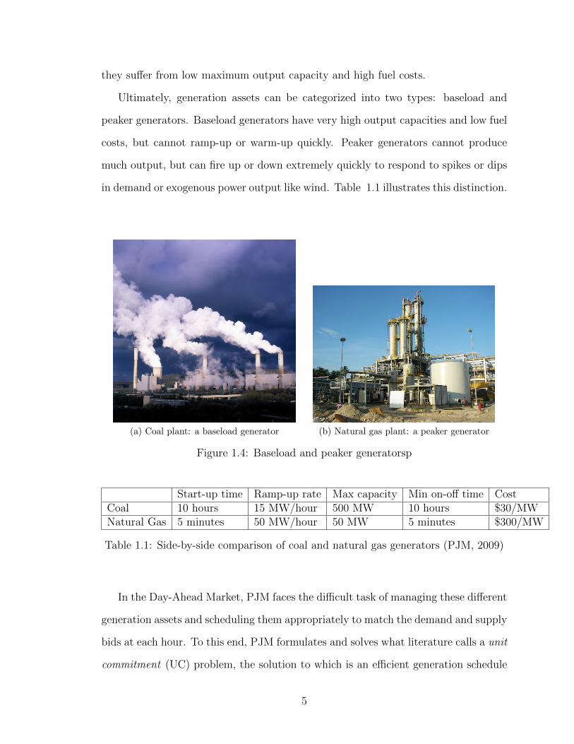
Ultimately, generation assets can be categorized into two types: baseload and
peaker generators. Baseload generators have very high output capacities and low fuel
costs, but cannot ramp-up or warm-up quickly. Peaker generators cannot produce
much output, but can fire up or down extremely quickly to respond to spikes or dips
in demand or exogenous power output like wind. Table 1.1 illustrates this distinction.
(a) Coal plant: a baseload generator (b) Natural gas plant: a peaker generator
Figure 1.4: Baseload and peaker generatorsp
Start-up time Ramp-up rate Max capacity Min on-off time CostCoal 10 hours 15 MW/hour 500 MW 10 hours $30/MWNatural Gas 5 minutes 50 MW/hour 50 MW 5 minutes $300/MW
Table 1.1: Side-by-side comparison of coal and natural gas generators (PJM, 2009)
In the Day-Ahead Market, PJM faces the difficult task of managing these different
generation assets and scheduling them appropriately to match the demand and supply
bids at each hour. To this end, PJM formulates and solves what literature calls a unit
commitment (UC) problem, the solution to which is an efficient generation schedule
5

for the next operating day. Then for each node in the power grid, the Day-Ahead
locational marginal prices (LMPs) are calculated. These are the buying and selling
prices for each megawatt of power that is agreed upon in the Day-Ahead Market. PJM
posts LMPs by 4 pm, and then from 4 pm to 6 pm, additional offers may be made or
modified in PJM’s Balancing Market. After this point, PJM makes additional runs
of its UC model to optimize next day’s generation allocation.
1.2. Real-Time Energy Rebalancing
Even after solving the UC problem, PJM still needs to tune its generator allocation
in real-time to better reflect actual market conditions. Currently, the main source
of uncertainty in the PJM Day-Ahead Market is the demand curve; a an energy
consumer’s demand bid from the previous day may not accurately reflect the actual
demand needed for the current day. Figure 1.5, which plots hour-by-hour actual
demand and demand forecasts from 2009 PJM data, illustrates this perfectly.
Figure 1.5: Hourly actual/predicted demand comparison from 2009 PJM data
6

Since the Day-Ahead scheduling will map generation to the predicted demand
and not the actual demand, PJM must take steps to correct the discrepancies. Once
the actual demand becomes known in real-time, PJM will fire up/down its peaker
generators depending on whether the demand prediction was higher or lower than
the actual. While baseload generators can ramped up/down as well, they do so at
a much slower rate, which makes them less suitable for real-time adjustments. In
general, the generators with the cheapest fuel costs are ramped first in the act of re-
balancing. However, ramp-rates must also be considered here, because the generators
with the cheapest fuel costs tend to have the slowest ramp rates. Once the real-time
rebalancing is complete, PJM calculates the Real-Time LMPs, which are the buying
and selling prices for each megawatt of energy calculated in real-time (PJM, 2009).
The real-time adjustments will become more difficult in the presence of increased
wind, since wind is a greater source of volatility and stochasticity than demand. In
reality, it is difficult to predict how increased wind penetration will affect PJM’s real-
time rebalancing. As of 2010, the level of wind energy constitutes only 0.5% of the
total generation in the PJM grid, which means that currently, wind fluctuations have
little to no affect on the system. However, this will no longer be the case as wind’s
total contribution to the system increases.
1.3. Offshore Wind Energy
As stated earlier, the US is beginning to develop significant capacity for wind energy.
However, from the viewpoint of a grid operator like PJM, the total capacity is not
indicative of wind energy’s potential. Instead, PJM needs to consider the locations
where wind energy is abundant. After all, grid operators must manage its transmis-
sion costs and ensure that the grid is not overloaded. Even if a stretch of land enjoys
high levels of wind, the transmission costs will be too high for PJM if that location is
7

too far away from its main grid. In addition, transmitting electricity from a faraway
location can put too much stress on the power lines, which is highly undesirable for
PJM.
Figure 1.6: Map of wind energy and transmission grid in the US (NREL, 2008)
As seen in Figure 1.6, the Midwest is the only part of the US with significant levels
of wind. However, that area serves little interest to PJM since its main jurisdiction
is at the Pennsylvania-Jersey-Maryland area near the east coast. PJM’s service does
extend into Illinois somewhat, as seen in Figure 1.3, but trying to transmit wind
energy from there could be cost-prohibitive. Ultimately, from PJM’s standpoint, the
best source of wind energy seems to be from the east coast. As evidenced by the map,
the offshore wind capacity along the east coast is quite staggering.
Unsurprisingly, this potential has not gone unnoticed. The Trans-Elect Develop-
ment Company has proposed an electrical transmission backbone along the east coast
to tap into its significant amount of wind energy. Funded by large private investors
8
like Google, this project, called the Atlantic Wind Connection (AWC), is set to be-
gin construction in 2013. Once completed, the AWC line will span 350 km along
the Mid-Atlantic coast. The initial phase of the project is set to connect population
and power transmission hubs in souther New Jersey and Reheboth Beach, Delaware.
When fully completed, the AWC will use 350 miles of cable as a backbone to deliver
power to southern Virginia and northern New Jersey as well. Estimates place the
total capacity of the AWC to be around 7000 MW, which is sufficient to power 1.9
million homes along the serviced areas (AWC 2011).
Needless to say, the injection of offshore wind will add a huge layer of stochasticity
to PJM’s energy market operations. In effect, PJM will need to face stochastic
elements from the supply side of its energy market as well as from the demand side.
Unfortunately, wind is extremely difficult to predict accurately, which makes PJM’s
UC problem even more challenging.
Other than finding accurate methods for wind prediction, an approach the grid
operator could take is to find ways to smooth out the volatility of wind. One of such
methods is the use of energy storage, like hydroelectric batteries. During high periods
of wind, the excess generation can be pumped into storage for later use during low
periods of wind. However, finding an optimal policy to implement this general idea
is an entire problem class altogether. Thus, this thesis focus more on dealing with
wind’s stochasticity, rather than its volatility.
If harnessed efficiently, offshore wind, because of its zero marginal cost, could
help PJM and other grid operators to save generation costs. However, a UC model
that does not assume wind penetration will not be able to handle the huge volatility
and stochasticity of wind. It will mostly likely result in overproduction during high
periods of wind, and shortages at low periods of wind. Overproduction obviously
leads to unnecessary cost, and shortages will force PJM to ramp up their expensive
peaker plants, which would also greatly increase cost of generation. Overall, accurate
9

wind predictions and a well-formed UC model are key to solving this problem.
1.4. Thesis Overview
This thesis will first summarize the main methods of solving the UC problem in
Chapter 2. Chapter 3 will give a quick overview of the data that serve as inputs
into the UC Model proposed in this thesis. Then, Chapter 4 will give a formulation
of PJM’s UC Model, the results of which are then discussed in Chapter 5. Finally,
Chapter 6 will give final remarks and comment on further areas of research.
10

Chapter 2
Unit Commitment Literature
Review
In order to meet the demand at every hour, PJM seeks to find the optimal allocation
among all of its generators. However, many generators have limitations from their
start-up time, ramp-up rates, minimum on/off time, etc. To solve this problem
given these constraints, PJM faces a unit commitment (UC) problem. The following
sections will review some methods for solving such a problem.
2.1. Mixed-Integer Programming
Mixed integer programming (MIP) is one of the most practical and popular ways of
solving the UC problem, especially given the advent of software packages like CPLEX
that can solve MIPs quickly. MIPs are much like regular linear programs, but the key
difference is that MIPs contain a mix of integer and non-integer variables. A sample
formulation is as follows (Yan & Stern, 2002):
11

Decision variables
uti =
1 if generator i is on at time t
0 otherwise
yti =
1 if generator i started up at time t
0 otherwise
zti =
1 if generator i shut down at time t
0 otherwise
pti = Output (in MW) of generator i at time t
Generator parameters
fi(pti) = Fuel cost of unit i at time t with generation of pti
pi
= Minimum capacity for generator i
p̄i = Maximum capacity for generator i
Cu,i = Start-up cost for generator i
Cd,i = Shut-down cost for generator i
Ru,i = Ramp-up rate for generator i
Rd,i = Ramp-down rate for generator i
Ui = Minimum on time for generator i
Di = Minimum off time for generator i
12
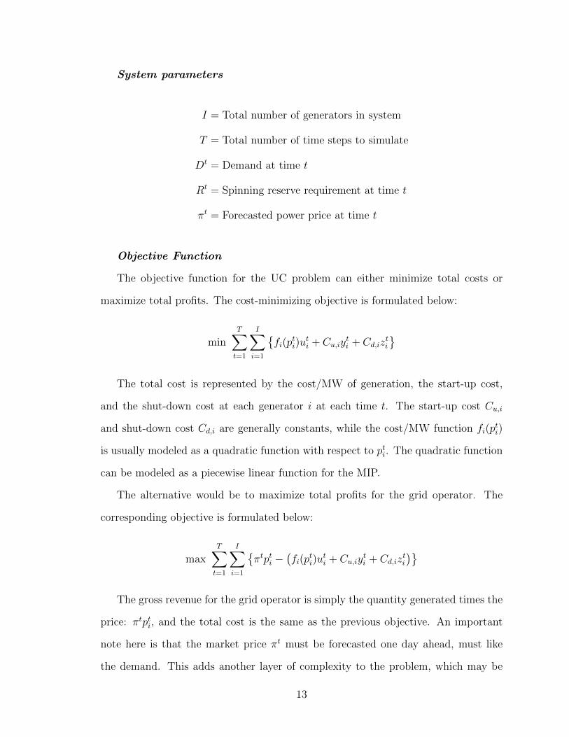
System parameters
I = Total number of generators in system
T = Total number of time steps to simulate
Dt = Demand at time t
Rt = Spinning reserve requirement at time t
πt = Forecasted power price at time t
Objective Function
The objective function for the UC problem can either minimize total costs or
maximize total profits. The cost-minimizing objective is formulated below:
minT∑t=1
I∑i=1
{fi(p
ti)u
ti + Cu,iy
ti + Cd,iz
ti
}The total cost is represented by the cost/MW of generation, the start-up cost,
and the shut-down cost at each generator i at each time t. The start-up cost Cu,i
and shut-down cost Cd,i are generally constants, while the cost/MW function fi(pti)
is usually modeled as a quadratic function with respect to pti. The quadratic function
can be modeled as a piecewise linear function for the MIP.
The alternative would be to maximize total profits for the grid operator. The
corresponding objective is formulated below:
maxT∑t=1
I∑i=1
{πtpti −
(fi(p
ti)u
ti + Cu,iy
ti + Cd,iz
ti
)}The gross revenue for the grid operator is simply the quantity generated times the
price: πtpti, and the total cost is the same as the previous objective. An important
note here is that the market price πt must be forecasted one day ahead, must like
the demand. This adds another layer of complexity to the problem, which may be
13
undesirable.
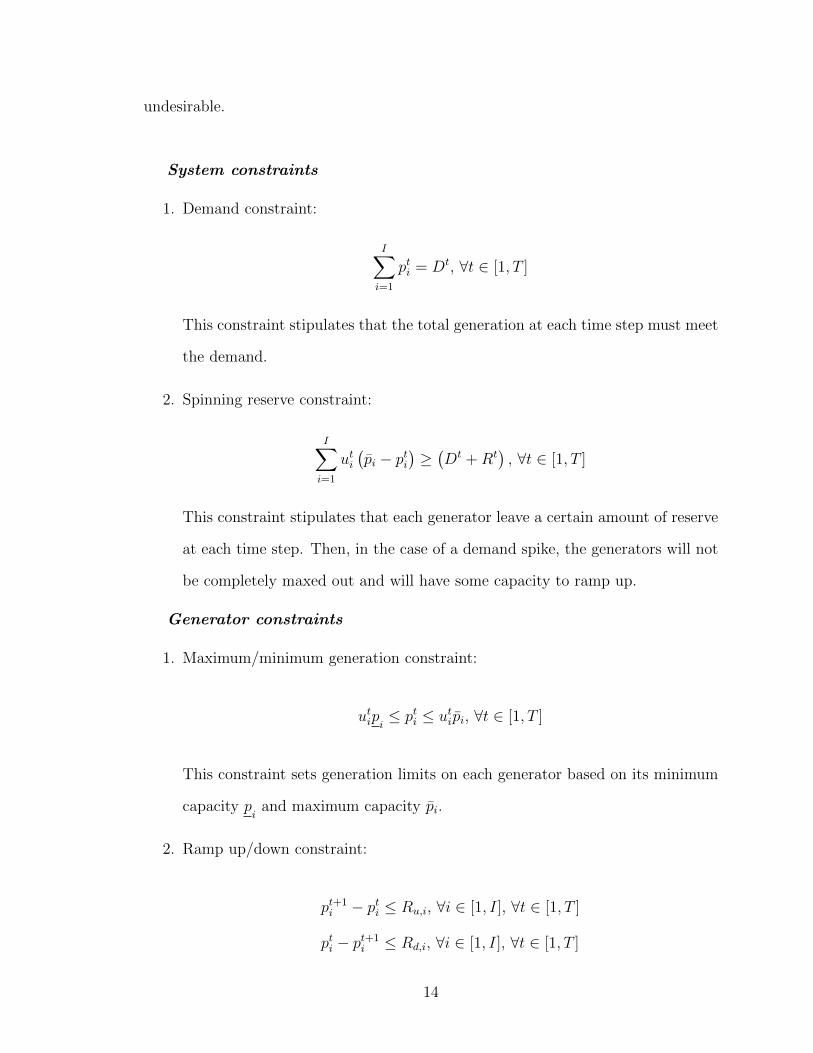
System constraints
1. Demand constraint:
I∑i=1
pti = Dt, ∀t ∈ [1, T ]
This constraint stipulates that the total generation at each time step must meet
the demand.
2. Spinning reserve constraint:
I∑i=1
uti(p̄i − pti
)≥(Dt +Rt
), ∀t ∈ [1, T ]
This constraint stipulates that each generator leave a certain amount of reserve
at each time step. Then, in the case of a demand spike, the generators will not
be completely maxed out and will have some capacity to ramp up.
Generator constraints
1. Maximum/minimum generation constraint:
utipi ≤ pti ≤ utip̄i, ∀t ∈ [1, T ]
This constraint sets generation limits on each generator based on its minimum
capacity pi
and maximum capacity p̄i.
2. Ramp up/down constraint:
pt+1i − pti ≤ Ru,i, ∀i ∈ [1, I], ∀t ∈ [1, T ]
pti − pt+1i ≤ Rd,i, ∀i ∈ [1, I], ∀t ∈ [1, T ]
14

These constraints limits how much power generation can change from one time
period to the next depending on the generator’s ramp-up rate Ru,i and ramp-
down rate Rd,i.
3. Start-up constraint:
uti − ut−1i = yti − zti , ∀i ∈ [1, I], ∀t ∈ [2, T ]
yti + zti ≤ 1, ∀i ∈ [1, I], ∀t ∈ [1, T ]
These constraints prevent generators from shutting down and starting up in the
same time step, and handles the transition between shutting down and starting
up.
4. Minimum on/off time constraint:
yti +
t+Ui−1∑k=t+1
zki ≤ 1, ∀i ∈ [1, I], ∀t ∈ [1, T ]
zti +
t+Di−1∑k=t+1
yki ≤ 1, ∀i ∈ [1, I], ∀t ∈ [1, T ]
These constraints prevent generators from shutting down immediately after
starting up, and vice versa. Once started up, the generator must stay on for
minimum on time Ui. In the opposite case, the generator must stay shut down
for minimum down time Di.
These objectives and constraints complete the sample formulation of the UC prob-
lem. Other formulations include the effect of government subsidies, breakdown of
power plants, disruptions in transmission, etc. The MIP model presented in this
thesis will not consider these rare, random events. The model will be similar to this
sample, but with some key additions and modifications.
15

2.2. Priority Listing
The priority listing method sorts every generator in a system with some priority
heuristic, and then commits each generator in sequence to fill out the demand curve.
This algorithm can be an effective way to circumvent one of the main weaknesses of
the MIP: infeasibility. An MIP formulation with many constraints can have difficulties
finding a feasible solution. In addition, depending on the complexity of the model,
MIP formulations can take a significant amount time to output a solution. Priority
lists will never run into these problems, and can yield near-optimal solutions if the
sorting heuristic is reasonably formed.
A simple formulation of this algorithm is as follows (Tingfang & Ting, 2008).
First, define the parameters below:
Pmaxi = Maximum capacity of generator i
Fi(Pi) = Fuel cost function of generator i with output Pi
= αi + βiPi + γiP2i where αi, βi, and γi are constants
First, generators with the higher capacity will be given higher priority. If genera-
tors share the same maximum capacity, then the one with the lower heat rate (HR)
will be given higher priority. The heat rate is calculated with the following equation:
HRi =Fi(P
maxi )
Pmaxi
Note that the heat rate is simply the fuel cost at a generator’s maximum capacity
weighted by the maximum capacity. The heat rate, instead of the strict fuel cost,
is often used in priority listing algorithms because it is the industry standard in
measuring how efficiently a generator used heat energy (Tingfang & Ting, 2008).
Placing priority on fuel cost alone may cause generators with low capacities to be
16

ranked higher than those with higher capacities. This can often lead to inefficient
solutions, especially if the low-capacity generators have a non-zero minimum on/off
time.
Once the generators are sorted by this priority heuristic, they are committed in
sequence to fill the demand curve. When being committed, the generators are still
subject to limitations like start-up time, ramp-up rate, minimum on time, etc. While
the priority listing algorithm is relatively simple, its results tend to be sub-optimal
when compared to the MIP, which tends to allow more complex, and thus more
realistic, formulations. Due to the existence of fast solvers like CPLEX and the fact
that well-formed MIPs should not be infeasible anyways, MIPs still remain one of
the most popular methods of solving the UC problem. Despite this fact, this thesis
will still use a modified version of this priority listing algorithm to implement its
simulation of real-time energy rebalancing.
2.3. Lagrangian Relaxation
The Lagrangian relaxation method basically solves the dual of the UC problem with
relaxed constraints. First, consider the demand and reserve constraints for the UC
problem, reproduced below (Che & Tang, 2009):
I∑i=1
pti = Dt, ∀t ∈ [1, T ]
I∑i=1
uti(p̄i − pti
)≥(Dt +Rt
), ∀t ∈ [1, T ]
Now, the Lagrangian function L can be defined as below:
L(~p, ~u,~λ, ~µ) = φ(~p, ~u) +T∑t=1
λt
(Dt −
I∑i=1
pti
)+
T∑t=1
µt
(Dt +Rt −
I∑i=1
uti(p̄i − pti
))
17
where ~λ = (λ1, ..., λT )T and ~µ = (µ1, ..., µT )T are the Lagrangian multipliers to the
two constraints. These variables serve to relax the constraints of the original problem.
Then this relaxed dual problem can be formulated as below:
max θ(~λ, ~µ)
s.t. ~µ ≥ 0
where θ(~λ, ~µ) = min~p,~u
{L(~p, ~u,~λ, ~µ)|(~p, ~u) ∈ Ui, i ∈ I
}. Here, Ui is the solution space
for ~p and ~u such that they satisfy all the other constraints in the UC problem, like
the maximum/minimum capacity constraint, ramp-up constraint, etc.
Solving this dual problem constructs the feasible, and possibly optimal, solution
~p, ~u. Lagrangian relaxation can also be used to divide a large UC problem into smaller
sub-problems, which can be solved individually as above. In addition, the relaxed
constraints mean that the Lagrangian Relaxation method is more likely to lead to
a feasible solution than the MIP. While Lagrangian Relaxation remains a popular
method of solving the UC problem, the advent of fast and reliable MIP solvers have
created a tendency to formulate the UC problem as a MIP instead of a Lagrangian
relaxation problem.
2.4. Additional Complexities
The methods covered in this chapter are perhaps the most common methods of solving
the UC problem. However, the formulations given above are deceptively simple; one
could possibly add additional complexities to the models to get more realistic results.
One factor that could be added is thermal states. Depending on the number of
hours that a generator has been on, its thermal state shifts from ”cold” to ”warm” to
”hot”. Intuitively, the start-up costs and marginal costs can be modeled as a function
of these thermal states; A ”cold” generator that has not been started for a long time
18

will obviously take more fuel to turn on than a ”hot” generator that has only been
shut down for a short time.
Another thing to note is that the generator constraints given in the first sub-
section may not suffice as general constraints. Different types of generators may be
governed by different constraints. For example, a hydro plant, along with its start-
up and ramp-up constraints, may also be subject to unique water flow and balance
constraints. Another exception to the constraints is the steam plant, which does not
have a uniform ramp-up rate. Steam plants are attached to ”fast” combustion tur-
bines, and thus cannot start ramping up unless the turbines start up and reach a
certain level of generation. At this point, the ramp-up rate of the steam plant would
depend on the thermal state of the turbine, which makes modeling such generators
quite complicated.
For the sake of tractability and simulation run-time, the model presented in Chap-
ter 4 will not include many of these additional complexities. Simplifying assumptions
and alternative formulations of some of these complexities will be presented in the
Chapter 4 as well.
19
Chapter 3
Data Overview
In order to formulate the UC Model, real generator, load, and wind data are used
as inputs. The generator and load data were provided by PJM and Ventyx, and the
wind data was provided by Stanford University. Sections 3.1, 3.2, 3.3 detail the
generator data, load data, and wind data, respectively.
3.1. Generator Data
The primary source of generator data in this thesis is the bid data provided by
PJM, which provides information on generator parameters like ramp rates, warm-up
times, and bid prices at hourly increments. The most important parameter to extract
from this data set is the bid price for each generator. As detailed in Chapter 1,
the amalgamation of the bids from energy consumers forms a cost curve for each
generator. These bid curves serve as the generator cost inputs into PJM’s UC Model
and are updated every hour as the bids change. The model implemented in this thesis
will do the same, with additional assumptions, as explained in Chapter 4. Updating
the bids at every hour as such gives the allows the UC Model here to accurately reflect
the dynamics of PJM’s Day-Ahead Market.
While bid prices should be updated at every hour, the same logic does not apply
20

for physical parameters like ramp rates and warm-up times. In PJM’s Day-Ahead
Market, it is possible for bids at certain hours to set certain ramp rates at 0 MW/hour,
or warm-up times to 0 hours. Such glitches in the bid data occur for generators that
have been on for some time; if a generator has already been on for several hours
at time t, it is feasible for the current Day-Ahead Market to set the ramp rate and
warm-up times as such at time t. Unfortunately, allowing this phenomenon in the
UC Model would skew the results, because the slow, baseload plants may be able to
ramp and warm up/down with little cost. For this reason, the physical parameters of
the PJM generators are pulled from a separate data set from Ventyx. A one-to-one
mapping between these two data sets was difficult to achieve, and some generators
were inevitably dropped in the process.
Generator Type Steam Nuclear CT Landfill Diesel Hydro Max Capacity (MW)Before Ventyx 708 51 952 43 74 82 294073.1After Ventyx 525 47 738 1 6 10 233351.283
Table 3.1: Tally of generation assets before and after Ventyx integration
Figure 3.1: Comparison of generation mixture before and after Ventyx integration
21
While the difference in total number of generators seems rather serious, the percent
difference in total maximum capacity turns out to be around 20%, which is within an
acceptable range. Furthermore, as evidenced by Figure 3.1, the distribution of the
total generation capacity is quite similar in both cases. Since the updated generator
parameters of the Ventyx data are more accurate than those of the PJM bid data,
this integrated data set will be used in the UC Model presented in this thesis.
3.2. Demand Data
For this thesis, PJM provided two sets of demand data: a time series of the aggregate
demand along with a corresponding time series of demand predictions, and a set
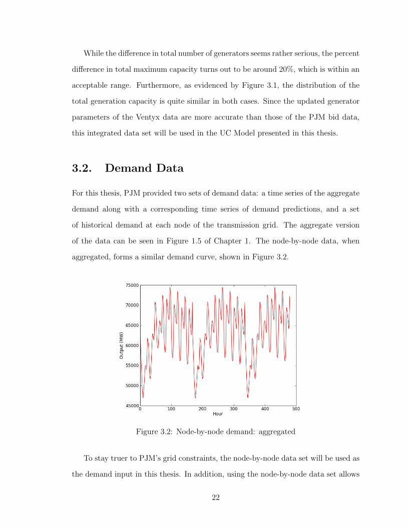
of historical demand at each node of the transmission grid. The aggregate version
of the data can be seen in Figure 1.5 of Chapter 1. The node-by-node data, when
aggregated, forms a similar demand curve, shown in Figure 3.2.
Figure 3.2: Node-by-node demand: aggregated
To stay truer to PJM’s grid constraints, the node-by-node data set will be used as
the demand input in this thesis. In addition, using the node-by-node data set allows
22
the model to filter out nodes that did not map to the current generator data set or
nodes with corrupted data. The unfortunate side effect is that prediction data was
not available in a node-by-node basis, which means that the aggregate demand must
be deterministic in this model. With the other data set, the discrepancy between the
actual demand and predicted demand stayed close to around 10%. This thesis will
assume this error margin small enough that assuming deterministic demand will not
skew the results significantly. This leaves wind as the main source of stochasticity in
this thesis. Wind is significantly more volatile and stochastic than demand, which
also supports the deterministic assumption.
3.3. Wind Data
The wind data for this thesis was provided by Stanford University, and consists of 6
offshore wind farms off the northeast coast of the US More specifically, the locations
represented are Martha’s Vineyard, Block Island, Long Island, and Nantucket. The
other 2 offshore wind farms are simulated data based on the wind from these 4
locations. The current wind data set contains the output (in MW) of each wind farm
at every hour in January, 2010 for one month. Figure 3.3 on the next page displays
the output of each farm at each hour.
23

Figure 3.3: Outputs of 6 offshore wind farms on the US east coast
24

Because these sample wind farms are clustered in the northeast coast of the U.S,
one may notice that the wind time series for all of them move quite similarly. In
other words, all 6 wind outputs tend to spike and dip at the same time. The side
effect of this trend is that the aggregate wind in the UC Model is much more volatile.
One way to offset aggregate wind volatility would be to pick more wind farms from
different locations, but this is not possible given the current wind data set.
The 3 levels of wind penetration explored in this thesis will be 5%, 20%, and
40%. To calibrate the wind data for these cases, the outputs of the 6 wind farms
are aggregated, and then compared against the total load in a simulation run. The
percentage of the total load that comes from wind output is then set as the wind level.
To achieve different values for the wind penetration, the aggregate wind was scaled
by a constant in each case. The results of this scaling can be seen in Figure 3.4.
Figure 3.4: Aggregate wind output
In this thesis, these aggregated wind time series are then used to make day-ahead
25

predictions for the Day-Ahead UC Model. Wind predictions for hour t of the next
day is derived from the wind output at the corresponding hour from the previous
seven days. At each hour, the q quantile of the wind at the same hour for the past
7 days is set to be the predicted wind. Figure 3.5 compares the wind prediction and
the actual wind in the 20% wind case for 3 values of q: 0.3, 0.5, and 0.7.
(a) q = 0.3 (b) q = 0.5
(c) q = 0.7
Figure 3.5: Wind predictions at different values of q
As observed here, increasing the quantile value q tends to increase the wind pre-
dictions. Considering that the predicted wind is an input value to the Day-Ahead UC
Model, q, in one sense, serves as the measure of the model’s ability to utilize wind.
To restrict the Day-Ahead Model’s ability to use wind, one could pick a low value for
26

q, and vice versa if one wished to allow the model to use more wind. In Chapter 5,
the value of q will be tuned over several runs to minimize total simulation costs. As
it turns out, tuning q also proves to be vital for eliminating shortages as well.
27

Chapter 4
The Unit Commitment Model
This chapter will present a unit commitment model to solve PJM’s power allocation
problem. The proposed solution consists of two steps: the Day-Ahead model and the
Hour-Ahead model. The following sections will propose the mathematical formulation
of these two components.
4.1. The Day-Ahead Model
The Day-Ahead model will solve for an optimal generator allocation for the next day
with predictions serving as placeholders for actual demand and wind data. Some of
the constraints for this model will be taken from the sample formulation in Chapter
2, with several additions and modifications to account for the different assumptions
and data.
4.1.1 Model Assumptions
Modeling every intricacy in PJM’s Day-Ahead Market would result in an intractable
and most likely infeasible MIP. To avoid such problems, assumptions are necessary
to simplify the model. The following assumptions allow for a simpler model without
28

sacrificing the accuracy of the results.
1. The first and perhaps most important simplification made in this model is the
calculation of bid costs for each generator. As explained in Chapter 1, the
amalgamation of demand bids form a cost curve for each generator, an example
of which is shown in Figure 4.1.
Figure 4.1: Sample cost curve for a steam plant
Unfortunately, not all cost curves can be modeled as piece-wise linear function.
In addition, going through the piece-wise process for all of the PJM generators
would increase the runtime to unmanageable levels. Thus, this model uses an
averaged cost of operations for each generator. Let c(x) be the bid curve. In
addition, let pmin and pmax be the minimum and maximum capacity of the
generator, respectively. Then we calculate the average cost cavg as follows:
cavg =
∫ pmax
pminc(x)dx
pmax − pmin
29
This averaging scheme is reasonable given the monotonically increasing nature
of most generator cost curves. In addition, if a generator has a horizontal
bidding curve, this equation will still yield the corresponding constant cost.
It is important to note that this scheme is only used to solve the Day-ahead
MIP. When tallying total costs at the end of a simulation trial, the actual
generation cost (a.k.a. the fuel cost of generation) will be used. Using the actual
generation cost for the final cost calculation is much more accurate because for
many baseload generators like nuclear plants, it is common for the bid costs to
be 0.
2. This model does not differentiate between thermal states (“hot” and “cold”)
of generators, as explained in the previous section. This difference noticeably
affects only the baseload generators when they are turning on, and in most power
grid operations, this is generally a one-time event since baseload generators
usually do not turn off after turning on because of the time constraints. Thus,
eliminating this distinction saves runtime in running the MIP without affecting
the results significantly.
3. This model does not consider generator start-up costs when allocating output.
The main reason for this is that start-up costs depend on the current thermal
state of the generator, which this model will not include. The marginal cost (in
$/MW) of running a generator greatly exceeds its start-up cost, especially when
a generator is being run for an extended period of time, so this assumption most
likely will not have a significant impact on the results.
4. All of the renewable energy assets in the model (hydroelectric plants, wind
farms, etc) are assumed to have zero marginal cost. The marginal cost cal-
culations for renewable assets become extremely complex because their costs
rely heavily on atmospheric conditions like rainfall, temperature, river flow, etc.
30

Predicting these conditions is outside the scope of this paper. Fortunately, com-
pared to the cost of running non-renewable assets like coal plants, the marginal
costs of renewable energy is quite negligible.
5. This model does not consider supply-side forces in the PJM energy markets.
A major part of PJM’s operations is to match energy buyers with willing en-
ergy suppliers. Unfortunately, data critical for modeling the supply-side, like
minimum sell prices and past offer history, are some of PJM’s most confidential
information. To simplify matters and overcome this lack of data, this model
will assume that PJM can manipulate any generator necessary to fill out the
aggregated demand curve for the day.
6. In this model, the nuclear generators will start at their on states and remain
on for the entirety of the simulations. This assumption is made because many
of the nuclear generators in the PJM bid data did not map to the new Ventyx
data set, which means that their ramp rates and warm-up times are undefined.
While most generators that did not map to the Ventyx data were dropped,
the nuclear generators produce far too much baseload generation to be merely
dropped from the model. Since the nuclear generators cannot ramp up/down
very quickly anyways, it is reasonable for them to merely stay on for the entirety
of the simulation.
4.1.2 MIP Variables and Constraints
The list of variables that will be used in this UC model is listed in the subsequent
sections. Before moving onto the model, however, it is important to explain the
notation used for all the variable definitions.
Ultimately, the model presented in this chapter is an information process with a
31

lag. Hence, all decision variables will be denoted with the following notation:
xt,t′,i = Decision about generator i. Decision made at time t. Executed at time t′.
In its normal operations, PJM runs its day-ahead UC model at noon to make
decisions for the next day. So in the notation above, t will always be noon of the
current day, while t′ will be some hour between noon and midnight of the next day.
In this model, the times denoted by t′ will be indexed 1, ..., T , where T is the number
of time periods to solve for the next day (24 hours in this case). The subscript i
will be indexed 1, ..., I, where I is the number of non-renewable energy assets (coal
generators, steam plants, etc) in the system. Wind farms will be treated separately
since they cannot be directly controlled. Whenever wind farms are involved, the
decision variable will have the subscript j ∈ [1, J ], where J is the total number of
wind farms in the system.
32

4.1.2.1 Decision Variables
The variables listed below will be the ones being directly manipulated by the MIP
model to optimally allocate power generation.
ut,t′,i =
1 if generator i is on at time t′
0 otherwise
yont,t′,i =
1 if generator i was turned on at time t′
0 otherwise
yofft,t′,i =
1 if generator i was turned off at time t′
0 otherwise
wont,t′,i =
1 if generator i began warming up at time t′
0 otherwise
wt,t′,i =
1 if generator i is warming up at time t′
0 otherwise
pt,t′,i = MW of power generated by generator i at time t′
pt,t′,j = MW of power generated by wind farm j at time t′
The important distinction here is warming up a generator vs. turning on a gen-
erator. A generator must go through a warm-up period before it can actually turn
on to minimum capacity. Once turned on, the generator may begin ramping up its
output to reach the desired level.
33

4.1.2.2 Generator Parameters
These variables serve as mathematical descriptors for each generator.
pmini = minimum output capacity of generator i
pmaxi = maximum output capacity of generator i
τ oni = minimum on time for generator i
τ offi = minimum off time for generator i
∆upi = ramp-up time for generator i
∆downi = ramp-down time for generator i
Ci = marginal cost of operation for generator i (in $/MW)
These parameters will be drawn from PJM’s generator data. To find Ci, a bid
curve averaging scheme, as explained in Section 4.1.1, will be used to find a constant
operation cost for a given day. As such, Ci is the only generator parameter that
changes from day to day; the rest of the parameters should be constant throughout
the entire simulation.
4.1.2.3 End-of-day Generator Parameters
These variables denote the state of each generator at the end of a day. These param-
eters are carried over into the next day’s MIP to allow for reasonable transition in
34

generator states.
pt,i = output of generator i at the end of a day (in MW)
ut,i = on/off status of generator i at the end of a day
nt,i = number of hours that generator i has been on at the end of a day
mt,i = number of hours that generator i has been off at the end of a day
φont,i =
1 if generator i satisfies minimum on-time requirement at the end of a day
0 otherwise
φofft,i =
1 if generator i satisfies minimum off-time requirement at the end of a day
0 otherwise
wt,i = warm-up status of generator i at the end of a day
ot,i = number of hours that generator i has been warming up at the end of a day
ψwarmt,i =
1 if generator i satisfies minimum warm-up requirement at the end of a day
0 otherwise
These parameters are used in the next day’s MIP to construct transition con-
straints for the first hour.
4.1.2.4 System variables
These two variables represent the system components in this model.
Dt,t′ = total predicted demand to meet at time t′
pwindt,t′,j = predicted wind at time t′ at wind farm j
εt,t′ = slack term for the objective function
The total predicted demand values (Dt,t′) are acquired from PJM data, and the
35

predicted wind data (pt,t′,j) will be provided by a climate group at Stanford University.
The slack term (εt,t′), as seen in the objective function, is added to allow for the
total generation to be less than the total required demand in periods of low wind or
high demand without crashing the MIP. This term is penalized heavily to ensure the
optimality of the final solution.
4.1.2.5 Objective Function
This formulation will use a simple objective function for cost-minimization, as detailed
below:
min
{∑t′
∑i
Ci · pt,t′,i + Cunder · εt,t′}
As detailed in previous sections, Ci is the cost/MW of running generator i, and
pt,t′,i is the power output of generator i at time t′. εt,t′ is the amount by which the
total output is below the total demand at time t′. This term is penalized accordingly
with the weight Cunder, which is the cost of underage (in $/MW).
4.1.2.6 Generator Constaints
The following constraints for the MIP model physical constraints for the generators,
like warm-up time, maximum output, etc. In this section, I will denote the total
number of generators in the system, and T will denote the number of hours in the
optimization horizon (usually 24 hours in the UC problem).
1. Capacity constraint
pt,t′,i ≥ pmini · ut.t′,i, ∀i ∈ [1, I], t′ ∈ [1, T ]
pt,t′,i ≤ pmaxi · ut,t′,i, ∀i ∈ [1, I], t′ ∈ [1, T ]
36

These constraints ensure that pt,t′,i, the output of generator i at time t′, stays
within the output bounds of generator i, as defined by the maximum capacity
pmaxi and minimum capacity pmini .
2. On/off constraint
yont,t′,i + yofft,t′,i + wont,t′,i ≤ 1, ∀i ∈ [1, I], t′ ∈ [1, T ]
ut,t′,i − ut,t′−1,i = yont,t′,i + yofft,t′,i, ∀i ∈ [1, I], t′ ∈ [1, T ]
The first constraint here ensure that a generator cannot turn on, turn off, and
begin warming up within the same hour, and the second constraint ensure that
the decision variables are updated accordingly when a generator turns on or off.
3. Minimum on/off time constraint
yont,t′,i +
min(t′+τoni −1,T)∑t′′=t′+1
yofft,t′′,i ≤ 1, ∀i ∈ [1, I], t′ ∈ [1, T − 1]
yofft,t′,i +
min(t′+τoffi −1,T)∑t′′=t′+1
wont,t′′,i ≤ 1, ∀i ∈ [1, I], t′ ∈ [1, T − 1]
These constraints ensure that a generator does not stay on/off for more than
the allotted minimum on/off times (τ oni and τ offi ). These constraints only apply
if τ oni ≥ 1 and/or τ offi ≥ 1. Otherwise, these constraints will not apply to
generator i. Note that for the second constraint, wont,t′′,i is used instead of yont,t′′,i.
This formulation states that a generator cannot begin warming up until it has
been off for at least τ offi hours. Since a generator must warm up from its off
state before turning on, this effectively has the intended effect of making sure
that the a generator cannot turn on for at least τ offi hours after it turns off.
37
4. Warm-up constraint
wont,t′,i +
min(t′+τwarmi −1,T)∑
t′′=t′+1
yont,t′′,i ≤ 1, ∀i ∈ [1, I], t′ ∈ [1, T − 1]
wt,t′,i − wt,t′−1,i = wont,t′,i − yont,t′,i, ∀i ∈ [1, I], t′ ∈ [2, T ]
0 ≤ ut,t′,i + wont,t′,i ≤ 1 + yont,t′,i, ∀i ∈ [1, I], t′ ∈ [1, T ]
(1− ut,t′,i − wt,t′,i)− (1− ut,t′−1,i − wt,t′−1,i) = yofft,t′,i − wont,t′,i, ∀i ∈ [1, I], t′ ∈ [2, T ]
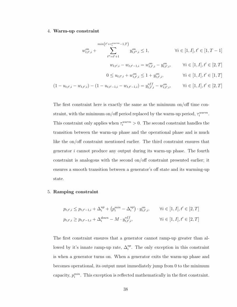
The first constraint here is exactly the same as the minimum on/off time con-
straint, with the minimum on/off period replaced by the warm-up period, τwarmi .
This constraint only applies when τwarmi > 0. The second constraint handles the
transition between the warm-up phase and the operational phase and is much
like the on/off constraint mentioned earlier. The third constraint ensures that
generator i cannot produce any output during its warm-up phase. The fourth
constraint is analogous with the second on/off constraint presented earlier; it
ensures a smooth transition between a generator’s off state and its warming-up
state.
5. Ramping constraint
pt,t′,i ≤ pt,t′−1,i + ∆upi +
(pmini −∆up
i
)· yont,t′,i, ∀i ∈ [1, I], t′ ∈ [2, T ]
pt,t′,i ≥ pt,t′−1,i + ∆downi −M · yofft,t′,i, ∀i ∈ [1, I], t′ ∈ [2, T ]
The first constraint ensures that a generator cannot ramp-up greater than al-
lowed by it’s innate ramp-up rate, ∆upi . The only exception in this constraint
is when a generator turns on. When a generator exits the warm-up phase and
becomes operational, its output must immediately jump from 0 to the minimum
capacity, pmini . This exception is reflected mathematically in the first constraint.
38

The second constraint follows the same idea, but covers the case of ramp-down.
In this case, the exceptional event that must be handled is when a generator
turns off. When a generator turns off, it is unplugged from the grid, and no
longer contributes any output. In mathematical terms, pt,t′,i must immediately
go to 0 in this case. To do this, let M be an arbitrarily large number, as ex-
pressed above. Then when a generator turns off yofft,t′,i, the ramp-down constraint
is slackened to allow this sudden output drop to occur.
4.1.2.7 End-of-day Transition Constraints
The following constraints apply only for the first hour of a day. They ensure that the
end-of-day parameters from the previous day are taken into account when starting a
new MIP for the current day.
1. Generator on/off transition constraint
ut,1,i − ut,i = yont,1,i − yofft,1,i, ∀i ∈ [1, I]
This is the exact same constraint as expressed in the previous section, except
at t′ = 1 and with the generator’s on/off status from the previous day, ut,i.
2. Minimum on/off time transition constraint
φont,i +
τoni −nt,i,T∑t′′=1
yofft,t′′,i ≤ 1, ∀i ∈ [1, I]
φofft,i +
τoffi −mt,i,T∑t′′=1
wont,t′′,i ≤ 1, ∀i ∈ [1, I]
These constraints are the same minimum on/off time constraints as expressed
in the previous section, except at t′ = 1. nt,i is the number of hours that a
39

generator has been on if it is still on at t′ = 1, and mt,i is the number of hours
that a generator has been off if it is still off at t′ = 1.
3. Ramping transition constraint
pt,1,i ≤ pt,i + ∆upi +
(pmini −∆up
i
)· yont,1,i, ∀i ∈ [1, I]
pt,1,i ≥ pt,i + ∆downi −M · yofft,1,i, ∀i ∈ [1, I]
These constraints are the same as the ramping constraints during the day, except
at t′ = 1. Here, pt,i is the output of generator i at the end of the previous day.
4. Warm-up transition constraints
ψwarmt,i +
min(τwarmi −ot,i,T)∑t′′=1
yont,t′′,i ≤ 1, ∀i ∈ [1, I]
wt,1,i − wt,i = wont,1,i − yont,1,i, ∀i ∈ [1, I]
(1− ut,1,i − wt,1,i)− (1− ut,i − wt,i) = yofft,1,i − wont,1,i, ∀i ∈ [1, I]
These are the same warm-up constraints as expressed in the previous section,
but at t′ = 1. The third warm-up constraint in the previous section does not
need a corollary here because it already covers the case of t′ = 1.
4.1.2.8 System Constraints
The following constraints for the MIP model the constraints to the system as a whole.
1. Demand constraint
∑i
pt,t′,i + εt,t′ ≥ Dt,t′ , ∀t′ ∈ [1, T ]
40

Here, Dt,t′ denotes the total energy demand (in MW) to be satisfied at time t′.
εt,t′ is an error term that allows this constraint to be satisfied even when the total
output is less than the total demand. With the increased presence of randomness
from wind, it is reasonable that the total output at time t′ may be less than the
amount needed. This error term prevents the MIP from becoming infeasible
in this case. To prevent this from undermining the solution’s optimality, it is
penalized accordingly in the objective function.
2. Reserves constraint
∑i
(pmaxi · ut,t′,i − pt,t′,i) ≥ ρ ·max(Dt,t′), ∀t′ ∈ [1, T ]
This constraint dictates that PJM’s generators cannot all be operating at max-
imum capacity. Instead, they must aggregately leave some capacity in reserve
to handle emergency demand spikes or dips in wind. The reserve capacity here
is specified by ρ ·max(Dt,t′). As specified by the North American Electric Re-
liability Corporation (NERC), grid operators must leave 1% of peak demand
forecasts in reserve at all times. In mathematical terms, this regulation sets
ρ = 0.01.
3. Wind constraint
0 ≤ pt,t′,j ≤ pwindt,t′,j (q), ∀j ∈ [1, J ], ∀t′ ∈ [1, T ]
In this model, wind farm outputs cannot be controlled directly. Instead, they
are at the mercy of the amount of wind at time t′. Here, wind predictions
for each wind farm j at each time t′ (denoted here by pwindt,t′,j (q)) is the upper
bound for the amount of output that the model can plan one day in advance.
Note that this term takes q, the quantile parameter discussed in Chapter 3, as
41

an argument because the wind predictions depend on the value of the quantile
chosen. The constraint allows the MIP to schedule less wind output than is
available; however, since wind energy has zero marginal cost in this model,
pt,t′,j will equal pwindt,t′,j (q) in most cases.
4.2. The Hour-Ahead Model
Because the results of the Day-Ahead model are based on predictions, discrepancies
between power generation and total demand are inevitable. The Hour-Ahead model
steps through the day hour-by-hour in real time and corrects these discrepancies by
ramping up/turning on the ”fast” generators accordingly. In day-to-day PJM op-
erations, this Hour-Ahead model consists of another MIP that schedules generators
hour-by-hour in 5 minute increments. Due to time constraints, this separate MIP
has not been integrated with the Day-Ahead model. Instead, the Hour-Ahead model
presented here will be an iterative algorithm quite similar to the priority listing al-
gorithm presented in Chapter 2. The following sections will give the mathematical
formulation of this model.
4.2.1 Model Assumptions
The assumptions from the Day-Ahead model still apply here. The additional assump-
tions for the Hour-Ahead model are listed below:
1. In real-time operations, PJM adjusts generator outputs in five-minute incre-
ments. However, due to the lack of sub-hourly wind and demand data, the
Hour-Ahead model here will need to plan in hourly increments. However, even
the baseload ”slow” plants in the PJM grid can ramp up considerably in an
entire hour, which would distort the results. Thus, the hour-ahead model com-
promises by allowing for 5 minutes of ramping per hour for each generator.
42

For example, if a generator has a ramp-rate of 60 MW/hour, it will be allowed
to ramp by 12 MW/hour in this model. With this formulation, the peaker
plants can still ramp quickly due to their extremely fast ramp rates, while the
slow plants will be much more limited, which accurately reflects their slow and
cumbersome nature. This distinction is visualized in Figure 4.2
(a) Baseload plants (b) Peaker plants
Figure 4.2: Histogram of ramp rates as a percentage of maximum capacity.
2. In their Hour-ahead model, PJM considers several variables like fuel cost, start-
up cost, and shutdown cost. However, only the fuel cost is reflected in this UC
model. Hence, the fuel cost will be the main factor in creating the priority list
of generators. Additional factors considered will be the minimum on/off times
of each generator. In general, units with lower minimum on/off times will be
favored in the priority list.
3. When firing up generators in the model, any plant with minimum on time
greater than 5 hours will not be allowed to turn on if it is off. This encompasses
most, if not all, of the baseload steam and nuclear plants, all of which have high
minimum on times. All plants with minimum on time less than 5 hours will be
prioritized according to the product of their minimum on time and fuel cost,
with the lowest products gaining the highest priority.
43
4. When turning down generators, any plant with minimum off time greater than
4 hours will not be allowed to turn off if it is on. Once again, this encompasses
most of the baseload plants, which tend to have high minimum off times. All
plants with minimum off times less than 4 hours will be prioritized according
to the product of their fuel costs and their minimum off times, with the lowest
values taking highest priority.
4.2.2 Model Variables
This subsection will list all of the variables necessary to run the Hour-ahead model.
Many of these variables are carried over from the Day-Ahead model, but many new
state and decision variables are introduced here.
4.2.2.1 State Variables
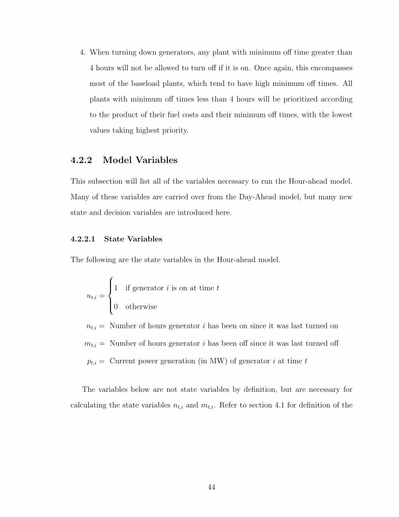
The following are the state variables in the Hour-ahead model.
ut,i =
1 if generator i is on at time t
0 otherwise
nt,i = Number of hours generator i has been on since it was last turned on
mt,i = Number of hours generator i has been off since it was last turned off
pt,i = Current power generation (in MW) of generator i at time t
The variables below are not state variables by definition, but are necessary for
calculating the state variables nt,i and mt,i. Refer to section 4.1 for definition of the
44

variables used here.
yont′,i, ∀t′ ∈ [t− τ oni , t] = Vector of yont′,i. Used with ut,i to calculate nt,i
yofft′,i , ∀t′ ∈[t− τ offi , t
]= Vector of yofft′,i . Used with ut,i to calculate mt,i
4.2.2.2 Decision Variables
The following are the decision variables in the Hour-ahead model. Note that the
decision variables in the Day-ahead model no longer apply in the Hour-ahead model.
xupt,i = Amount of power fired up by generator i at time t if there is supply shortage
xdownt,i = Amount of power turned down by generator i at time t if there is supply overage
The variables below are not decision variables themselves, but are vital for calcu-
lating xupt,i and xdownt,i .
Zshortt = Amount of supply shortage (in MW) at time t. Used to calculate xupt
Zovert = Amount of supply overage (in MW) at time t. Used to calculate xdownt
4.2.2.3 Exogenous Variables
The following are the exogenous variables in the Hour-ahead model.
D̂t = Actual power demand (in MW) at time t. Only known at time t′′ ≥ t
p̂t,wind = Actual wind output (in MW) at time t. Only known at time t′′ ≥ t
The data for D̂t was provided by PJM, while the data for p̂t,wind was provided by
Stanford University.
45

4.2.3 Decision Algorithms
The algorithm presented in this section details how to assign values to the decision
variables xupt,i and xdownt,i at a given time t. There are two cases to consider here: one in
which there is a supply shortage at time t, and one in which there is a supply overage
at time t. In both cases, the algorithms will use the generator parameter notation
introduced in Section 4.1.
4.2.3.1 Case 1: Supply Shortage
Algorithm 1 is the algorithm to run if there is a supply shortage at time t. It iterates
through the generator priority list and calculates xupt,i for each generator until the
shortage is eliminated.
Algorithm 1 Calculate xupt,i in the case of a supply shortage)
Require: Generators sorted in ascending order with respect to τ oni · CiZshortt = max
(D̂t − (
∑i pt,i + p̂t,wind) , 0
)while Zshort
t > 0 dofor all i ∈ I do
if ut,i == 1 then
xupt,i = min(pmaxi − pt,i, ∆up
i
12, Zshort
t
)else
if mt,i ≥ τ offi and τ oni ≤ 5 then
xupt,i = min(
max (min (pmaxi − pt,i) , pmini ) , Zshortaget
)end if
end ifZshortt = Zshort
t − xfiret,i
end forend while
The supply shortage at time t is calculated as the difference between the demand
at time t(D̂t
)and the total generation at time t (
∑i pt,i + p̂t,wind). While this
shortage is greater than 0 MW, Algorithm 1 loops through all the generators, which
are sorted in ascending order with respect to the product of the minimum on time
and the fuel cost (τ oni · Ci). If the current generator is still on (ut,i = 1), then the
46

generator can ramp up by the minimum of pmaxi − pt,i,∆up
i
12, and Zshort
t .∆up
i
12is the
amount that the generator can ramp in 5 minutes, as per the first assumption in
Section 4.2.1. The other quantities are added to handle edge cases. If the current
generator is off (ut,i = 0), then Algorithm 1 checks that it has been off for at least its
minimum off time (mt,i ≥ τ offi ), and that its minimum on time is less than 5 hours
(τ oni ≤ 5). If these conditions are met, the generator can turn on and fire output.
Algorithm 1 repeats this process until the shortage is eliminated or until there are no
more generators in the priority list.
4.2.3.2 Case 2: Supply Overage
Algorithm 2 should be run if there is a supply overage at time t. It goes through the
generator priority list and determines xdownt,i for each generator until the overage is
minimized.
Algorithm 2 Calculate xdownt,i in the case of a supply overage)
Require: Generators sorted in ascending order with respect to τ offi · CiZovert = max
((∑
i pt,i + p̂t,wind)− D̂t, 0)
while Zovert > 0 do
for all i ∈ I doif ut,i == 1 then
if nt,i ≥ τ oni and τ offi ≤ 4 then
xdownt,i = min(pt,i,−∆down
i
12, Zoverage
t
)else
if nt,i < τ oni or τ offi > 4 then
xdownt,i = min(pt,i − pmint,i ,−
∆downi
12, Zoverage
t
)end if
end ifend ifZovert = Zover
t − xdownt,i
end forend while
The supply overage at time t is calculated as the difference between the total
output (∑
i pt,i + p̂t,wind) and the actual demand at time t (D̂t). While this overage
47
is over 0 MW, Algorithm 2 iterates through the generator priority list. If the current
generator is on (ut,i = 1), then it can turn off if it has been on for at least its minimum
on time (nt,i ≥ τ oni ) and if its minimum off time is less than 4 hours (τ offi ≤ 4). In this
case, xdownt,i is calculated by similar logic as Algorithm 1. If the generator hasn’t been
on for at least its minimum on time (nt,i < τ oni ) or its minimum off time is greater
than 4 hours (τ offi > 4), then it can turn down, but not turn off completely. In this
case, the pt,i term in the min function is replaced by the term pt,i − pmint,i to prevent
the generator from completely turning off. Algorithm 2 stops when the overage is
eliminated or when there are no more generators in the priority list.
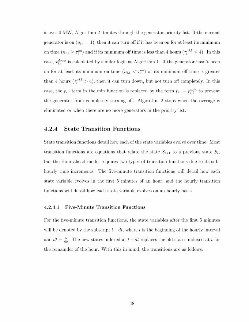
4.2.4 State Transition Functions
State transition functions detail how each of the state variables evolve over time. Most
transition functions are equations that relate the state St+1 to a previous state St,
but the Hour-ahead model requires two types of transition functions due to its sub-
hourly time increments. The five-minute transition functions will detail how each
state variable evolves in the first 5 minutes of an hour, and the hourly transition
functions will detail how each state variable evolves on an hourly basis.
4.2.4.1 Five-Minute Transition Functions
For the five-minute transition functions, the state variables after the first 5 minutes
will be denoted by the subscript t+dt, where t is the beginning of the hourly interval
and dt = 560
. The new states indexed at t+ dt replaces the old states indexed at t for
the remainder of the hour. With this in mind, the transitions are as follows.
48

pt+dt,i = pt,i + xfiret,i
ut+dt,i =
1 if pt+dt,i > 0
0 otherwise
yont+dt,i =
1 if pt,i > 0 and pt+dt,i > 0
yont,i otherwise
yofft+dt,i =
1 if pt,i > 0 and pt+dt,i = 0
yofft,i otherwise
nt+dt,i and mt+dt,i are in turn calculated from the updated values yont+dt,i and yofft+dt,i,
respectively.
4.2.4.2 Hourly Transition Functions
The transition functions here are hourly, where a decision in one hour affects the
state variable in the next hour. Due to the nature of unit commitment, formulating
transition functions at an hourly increment is a bit trickier than for the five-minute
case. According to the PJM Handbook, any generator that is assigned a non-zero
generation by the Day-Ahead model cannot deviate unless explicitly ordered by PJM.
This means that any generators that were committed by the Day-Ahead model must
readjust back to their planned output for time t + 1, regardless of how much they
ramped at time t in real-time. To model this realistically, the transition function
below only applies to generators that were not committed by the Day-Ahead model,
but were newly turned on by the Hour-Ahead model.
49

pt+1,i =
pt,i + xupt,i − xdownt,i if ut′,t,i = 0
pt′,t+1,i otherwise
If generator i was not planned at time t′ to be on at time t (ut′,t,i = 0), the power
output at time t + 1 is the output at time t plus however much the generator fired
up or down in real time. If generator i was planned at time t′ to be on at time t, it
must revert to the output planned at time t′ for time t+ 1 (pt′,t+1,i).
50

Chapter 5
Model Results and Discussion
This chapter will detail several outputs from the Day-Ahead and Hour-Ahead simu-
lations. First, the chapter will go over system summary plots at 5%, 20%, and 40%
wind penetration with the several values of q. The generation breakdown at each
wind level will be shown as well. Using these results, the parameter q will be tuned
at each level of wind penetration to minimize total cost. Finally, a case study will be
performed with deterministic wind to gauge the value of wind predictions.
5.1. Output Summary and Generator Breakdown
The summary plots in this section will include the total actual demand and the exact
breakdown of generationp types at each hour. For all plots, nuclear generation will
be denoted in blue, wind generation in green, steam generation in red, combustion
turbine (CT) generation in yellow, and all other generation in magenta. The total
demand to be met will be overlayed with a bolded line.
5.1.1 5% Wind
The summary plots with 5% wind penetration at each value of q are as follows.
51

(a) q = 0.1 (b) q = 0.2
(c) q = 0.3 (d) q = 0.4
(e) q = 0.5
Figure 5.1: 5% Wind UC Model Summary: q ∈ {0.1, 0.2, 0.3, 0.4, 0.5}
52

(a) q = 0.6 (b) q = 0.7
(c) q = 0.8 (d) q = 0.9
(e) q = 1.0
Figure 5.2: 5% Wind UC Model Summary: q ∈ {0.6, 0.7, 0.8, 0.9, 1.0}
53

The first trend to note is that the first day at all values of q suffer from shortages.
This occurs because in the beginning of the simulation, the baseload generators,
mainly the steam and nuclear plants, are still in the process of firing up and not
producing output yet. At all other periods, the system output fits the total demand
quite closely in all cases. In fact, the results don’t seem to be very different among
all the values of q. With wind output constituting only 5% of the total load, it is
possible that the stochasticity of wind does not have much effect in this case.
At all values of q, nuclear and steam plants constitute the majority of the gen-
eration, while the peaker plants (i.e. CT) kick in during periods of low wind. This
dynamic is illustrated in the close-up plot presented in Figure 5.3
(a) Close-up breakdown plot (b) Close-up wind plot
Figure 5.3: Close-up plot with 5% wind and q = 0.7
The wind throughout these 7 hours is extremely low, and the model has over-
predicted wind by approximately 5000 MW, as shown in the second subplot. As a
result, the model has consistently under-committed its baseload generators by 5000
MW. This gap must then be filled by the peaker plants in real time, which is reflected
in the first subplot. In general, scenarios as depicted in Figure 5.3 become more
common with higher values of q, which in turn leads to a greater presence of peaker
generation as q increases.
54

Figure 5.4: 5% wind: baseload and peaker generation percentages at each q
As demonstrated in Chapter 3, increasing q results generally results in higher wind
predictions, which would generally lead to the predicted wind being higher than the
actual wind. This would then cause the baseload generators to be under-committed in
the Day-Ahead model, which means that the peaker plants must fill in the difference
in the Hour-Ahead model. For the 5% case, however, the peaker generation is not
very significant, even at q = 1.0. The reasoning for this is that when wind, the
main source of stochasticity in the model, constitutes only 5% of the total load, it
probably will not have much of an impact on shortages in the Day-Ahead model.
The peaker generators become much more significant at higher levels of wind, where
under-predicting wind can actually cause severe under-commitments in generation.
5.1.2 20% Wind
The summary plots with 20% wind are presented below.
55

(a) q = 0.1 (b) q = 0.2
(c) q = 0.3 (d) q = 0.4
(e) q = 0.5
Figure 5.5: 20% Wind UC Model Summary: q ∈ {0.1, 0.2, 0.3, 0.4, 0.5}
56
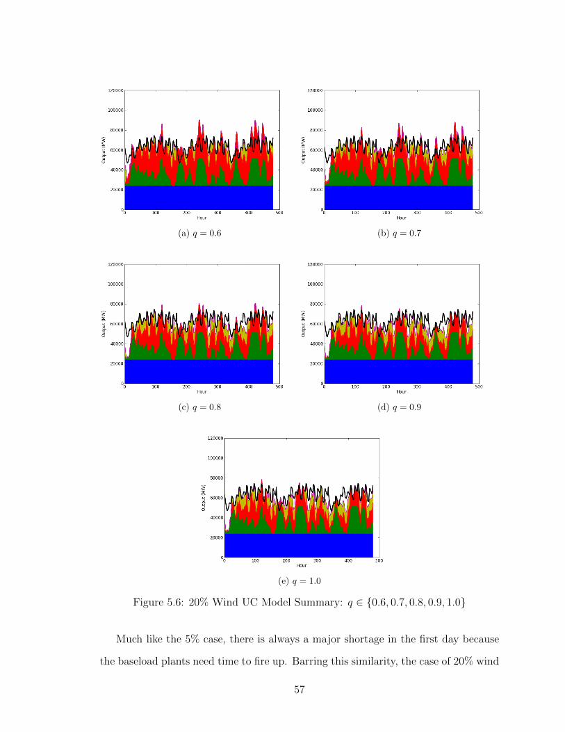
(a) q = 0.6 (b) q = 0.7
(c) q = 0.8 (d) q = 0.9
(e) q = 1.0
Figure 5.6: 20% Wind UC Model Summary: q ∈ {0.6, 0.7, 0.8, 0.9, 1.0}
Much like the 5% case, there is always a major shortage in the first day because
the baseload plants need time to fire up. Barring this similarity, the case of 20% wind
57
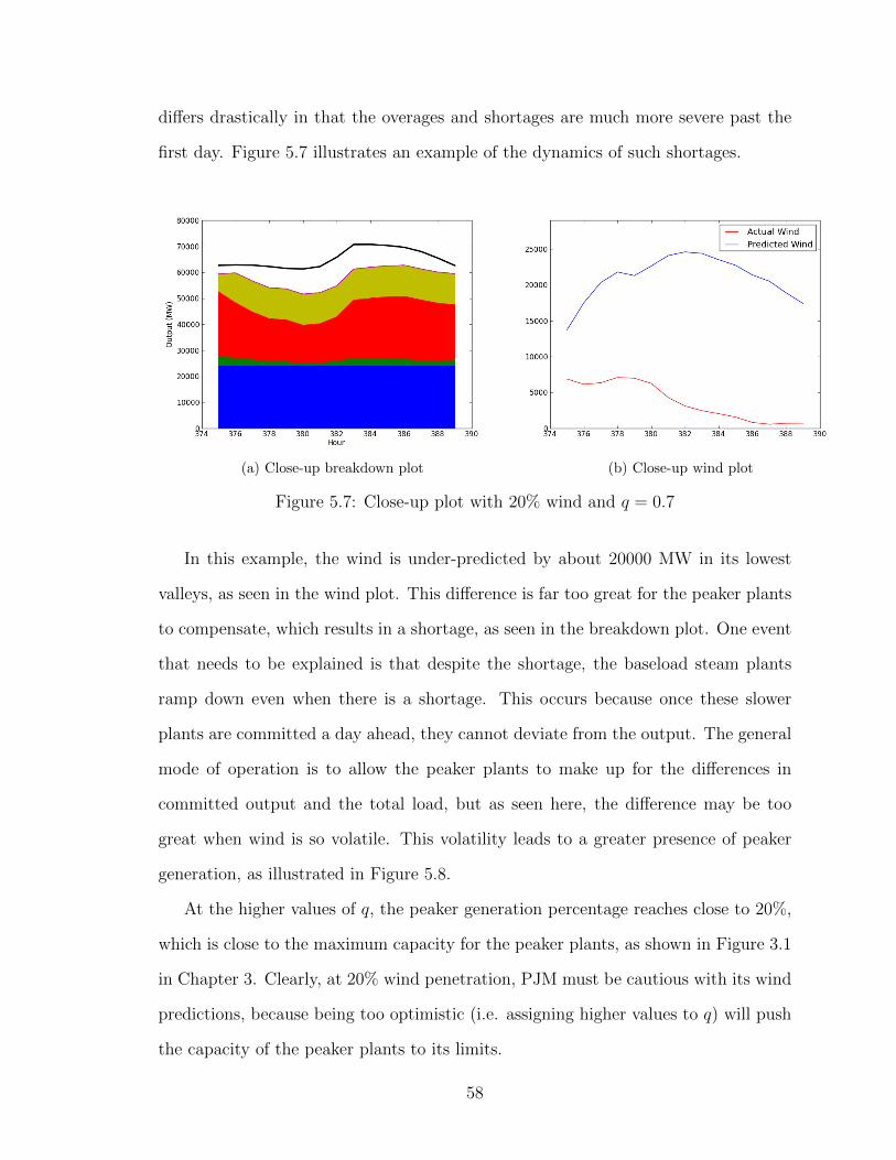
differs drastically in that the overages and shortages are much more severe past the
first day. Figure 5.7 illustrates an example of the dynamics of such shortages.
(a) Close-up breakdown plot (b) Close-up wind plot
Figure 5.7: Close-up plot with 20% wind and q = 0.7
In this example, the wind is under-predicted by about 20000 MW in its lowest
valleys, as seen in the wind plot. This difference is far too great for the peaker plants
to compensate, which results in a shortage, as seen in the breakdown plot. One event
that needs to be explained is that despite the shortage, the baseload steam plants
ramp down even when there is a shortage. This occurs because once these slower
plants are committed a day ahead, they cannot deviate from the output. The general
mode of operation is to allow the peaker plants to make up for the differences in
committed output and the total load, but as seen here, the difference may be too
great when wind is so volatile. This volatility leads to a greater presence of peaker
generation, as illustrated in Figure 5.8.
At the higher values of q, the peaker generation percentage reaches close to 20%,
which is close to the maximum capacity for the peaker plants, as shown in Figure 3.1
in Chapter 3. Clearly, at 20% wind penetration, PJM must be cautious with its wind
predictions, because being too optimistic (i.e. assigning higher values to q) will push
the capacity of the peaker plants to its limits.
58

Figure 5.8: 20% wind: baseload and peaker generation percentages at each q
Along with shortages, increasing the wind penetration to 20% leads to more no-
ticeable overages as well. The dynamics of overages are quite similar to those of
shortages. When the wind is under-predicted, the UC Model will over-commit its
baseload generators. Since baseload generators cannot ramp down significantly in
real time, this over-commitment leads to an output overage in most cases. This trend
is illustrated in Figure 5.9 on the next page.
59
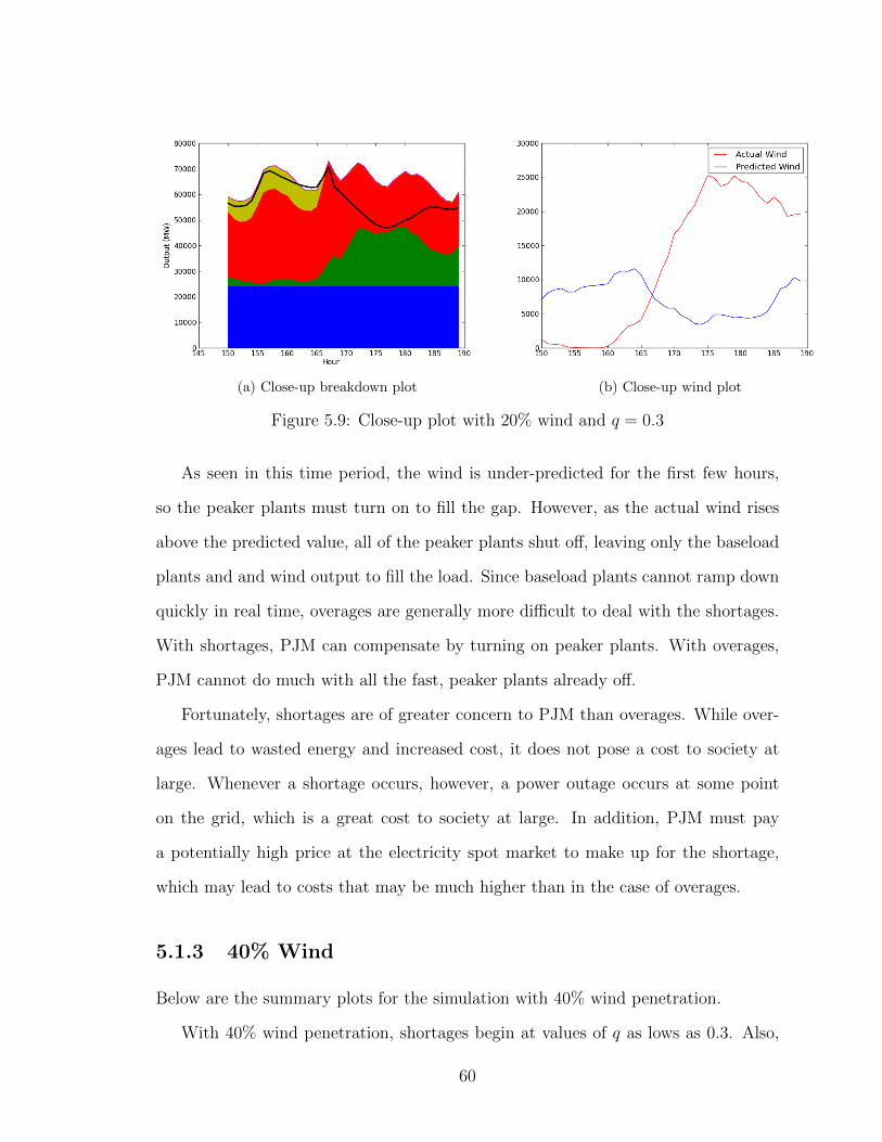
(a) Close-up breakdown plot (b) Close-up wind plot
Figure 5.9: Close-up plot with 20% wind and q = 0.3
As seen in this time period, the wind is under-predicted for the first few hours,
so the peaker plants must turn on to fill the gap. However, as the actual wind rises
above the predicted value, all of the peaker plants shut off, leaving only the baseload
plants and and wind output to fill the load. Since baseload plants cannot ramp down
quickly in real time, overages are generally more difficult to deal with the shortages.
With shortages, PJM can compensate by turning on peaker plants. With overages,
PJM cannot do much with all the fast, peaker plants already off.
Fortunately, shortages are of greater concern to PJM than overages. While over-
ages lead to wasted energy and increased cost, it does not pose a cost to society at
large. Whenever a shortage occurs, however, a power outage occurs at some point
on the grid, which is a great cost to society at large. In addition, PJM must pay
a potentially high price at the electricity spot market to make up for the shortage,
which may lead to costs that may be much higher than in the case of overages.
5.1.3 40% Wind
Below are the summary plots for the simulation with 40% wind penetration.
With 40% wind penetration, shortages begin at values of q as lows as 0.3. Also,
60

(a) q = 0.1 (b) q = 0.2
(c) q = 0.3 (d) q = 0.4
(e) q = 0.5
Figure 5.10: 40% Wind UC Model Summary: q ∈ {0.1, 0.2, 0.3, 0.4, 0.5}
for higher values of q, the UC Model does not plan that much steam generation, even
though the total output incurs a shortage. Figure 5.12 illustrates this result in greater
61

(a) q = 0.6 (b) q = 0.7
(c) q = 0.8 (d) q = 0.9
(e) q = 1.0
Figure 5.11: 40% Wind UC Model Summary: q ∈ {0.6, 0.7, 0.8, 0.9, 1.0}
detail
Note that the predicted wind in this case was in the 40000 MW to 60000 MW
62

(a) Close-up breakdown plot (b) Close-up wind plot
Figure 5.12: Close-up plot with 40% wind and q = 0.8
range, which is at the same order of magnitude as the total demand. Since the Day-
Ahead Model uses the wind prediction as an input, it does not schedule a significant
amount of steam generation, because it assumes that the high predicted wind will
cover most of the demand. However, this assumption does not hold true in real-time,
since the actual wind is much lower. Hence, the peaker plants need to fire up to
try and fill the demand, but there is not enough peaker capacity to do so completely.
Due to this phenomenon, peaker generation becomes much more prominent with 40%
wind, as evidenced by Figure 5.13.
63

Figure 5.13: 40% wind: baseload and peaker generation percentages at each q
These results make clear that the case of 40% wind suffers from the same problems
as 20% wind penetration, except more severe. This accentuates the fact that PJM
must be extremely careful with the choice of q, because picking a non-ideal value
for the parameter is more likely to cause severe load-shedding than with lower wind
levels. Picking the optimal value for q is the subject of Section 5.2.
5.2. Tuning q
To optimize the total cost and load-shed of the UC Model, the value of q must be
tuned. There are many criteria by which to tune this parameter; the model could
be tuned to minimize load-shedding (the occurrence of shortages and overages), or it
could be tuned to simply minimize the total fuel cost. Due to time constraints, the
model will be tuned based on the results for the 10 values of q presented in Section 5.1.
While more iterations would be necessary to reach a true optimum, the run-time of
the simulation would be too taxing. As usual, all simulations will be run at 3 different
64

levels of wind penetration: 5%, 20%, and 40%.
5.2.1 Tuning with Load-Shedding
This section will tune the UC model with respect to the amount of load shedding
at each value of q. Section 5.2.1.1 will show the total shortage from the simulation
at each value of q, and and Section 5.2.1.2 will detail the total overage. Finally,
Section 5.2.1.3 will detail how to pick the optimal q given the results.
5.2.1.1 Shortages
Table 5.1 and Figure 5.14 show the total output shortage as a percentage of the
total demand for the values of q and wind penetration. As shown in Section 5.1, the
baseload plants that typically make up the majority of power generation have not had
time to fire up during the first day. This means that in at all values of q and wind
penetration, shortages will be inevitable on the first day. To prevent this phenomenon
from skewing the results, the values presented below will omit the load-shed from the
first day.
Wind %/q 0.1 0.2 0.3 0.4 0.5 0.6 0.7 0.8 0.9 1.05% 0 0 0 0 0 0 0 0 0 020% 0 0 0 0 0.04 0.31 1.6 4.0 6.1 6.140% 0 0.02 0.3 0.83 2.1 5.4 10.8 16.9 21.7 21.7
Table 5.1: Total shortage % at different values of q
65

Figure 5.14: Shortage % at each value of q
As explored in Section 5.1, increasing q generally leads to greater shortages, be-
cause higher values of q imply a more optimistic prediction of wind, which would
inevitably mean that predictions will tend to be higher than the actual wind. This
is especially true for the case of 40% wind. Since the wind is scaled by a constant,
higher wind levels will observe much more volatility, which leads to greater shortages
with more optimistic predictions. This explains why shortages begin appearing so
early (at q = 0.3), with 40% wind. With 20% wind, shortages do not appear until
q = 0.6 and for 5% wind, there is simply no occurrence of shortages.
5.2.1.2 Overages
Table 5.2 and Figure 5.15 show the total overage as a percentage of the total demand
at different levels of wind. To remain consistent, the simulation results from the first
day have been discarded here as well.
66

Wind %/q 0.1 0.2 0.3 0.4 0.5 0.6 0.7 0.8 0.9 1.05% 5.6 4.9 4.1 3.4 2.9 2.4 1.9 1.5 1.2 1.220% 19.1 16.3 12.9 10.2 8.1 6.1 3.9 2.1 0.95 0.9240% 36.9 31.3 24.6 19 14.9 10.9 7.0 3.9 1.7 1.7
Table 5.2: Total overage % at different values of q
Figure 5.15: Overage % at each value of q
Intuitively, overages should decrease as q increases, which is the trend reflected
in Figure 5.15. Decreasing q means that the wind prediction will become more pes-
simistic, which means that the actual wind will tend to be greater than the predicted
value. This discrepancy scales much more drastically with 40% wind because of its
increased volatility, as reflected in Figure 3.4. Now that the results for shortage and
overage have been compiled, an optimal value for q can be picked, as explained in
Section 5.2.1.3.
67
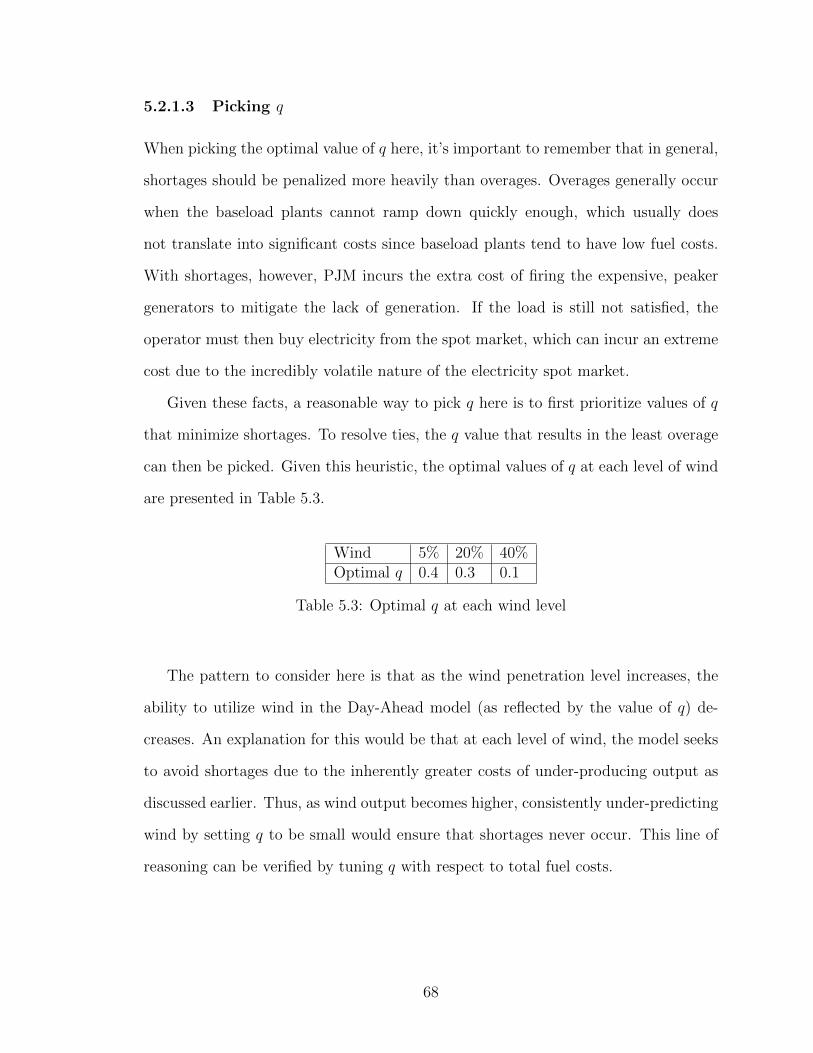
5.2.1.3 Picking q
When picking the optimal value of q here, it’s important to remember that in general,
shortages should be penalized more heavily than overages. Overages generally occur
when the baseload plants cannot ramp down quickly enough, which usually does
not translate into significant costs since baseload plants tend to have low fuel costs.
With shortages, however, PJM incurs the extra cost of firing the expensive, peaker
generators to mitigate the lack of generation. If the load is still not satisfied, the
operator must then buy electricity from the spot market, which can incur an extreme
cost due to the incredibly volatile nature of the electricity spot market.
Given these facts, a reasonable way to pick q here is to first prioritize values of q
that minimize shortages. To resolve ties, the q value that results in the least overage
can then be picked. Given this heuristic, the optimal values of q at each level of wind
are presented in Table 5.3.
Wind 5% 20% 40%Optimal q 0.4 0.3 0.1
Table 5.3: Optimal q at each wind level
The pattern to consider here is that as the wind penetration level increases, the
ability to utilize wind in the Day-Ahead model (as reflected by the value of q) de-
creases. An explanation for this would be that at each level of wind, the model seeks
to avoid shortages due to the inherently greater costs of under-producing output as
discussed earlier. Thus, as wind output becomes higher, consistently under-predicting
wind by setting q to be small would ensure that shortages never occur. This line of
reasoning can be verified by tuning q with respect to total fuel costs.
68
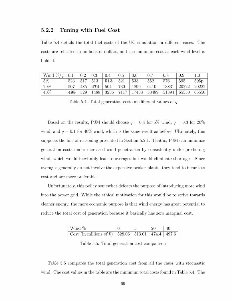
5.2.2 Tuning with Fuel Cost
Table 5.4 details the total fuel costs of the UC simulation in different cases. The
costs are reflected in millions of dollars, and the minimum cost at each wind level is
bolded.
Wind %/q 0.1 0.2 0.3 0.4 0.5 0.6 0.7 0.8 0.9 1.05% 523 517 513 513 521 533 552 576 595 595p20% 507 485 474 504 730 1899 6410 13831 20222 2022240% 498 529 1488 3256 7117 17433 33489 51394 65550 65550
Table 5.4: Total generation costs at different values of q
Based on the results, PJM should choose q = 0.4 for 5% wind, q = 0.3 for 20%
wind, and q = 0.1 for 40% wind, which is the same result as before. Ultimately, this
supports the line of reasoning presented in Section 5.2.1. That is, PJM can minimize
generation costs under increased wind penetration by consistently under-predicting
wind, which would inevitably lead to overages but would eliminate shortages. Since
overages generally do not involve the expensive peaker plants, they tend to incur less
cost and are more preferable.
Unfortunately, this policy somewhat defeats the purpose of introducing more wind
into the power grid. While the ethical motivation for this would be to strive towards
cleaner energy, the more economic purpose is that wind energy has great potential to
reduce the total cost of generation because it basically has zero marginal cost.
Wind % 0 5 20 40Cost (in millions of $) 528.06 513.01 474.4 497.6
Table 5.5: Total generation cost comparison
Table 5.5 compares the total generation cost from all the cases with stochastic
wind. The cost values in the table are the minimum total costs found in Table 5.4. The
69

total generation cost from a simulation with no wind is added for further comparison.
As seen here, there is a steady decrease in total cost with increasing wind until 20%.
At 40% wind penetration, the total cost actually increases from the 20% case. The
explanation for this phenomenon goes back to the fact that PJM wants to minimize
the occurrence of shortages. In that regard, the cost-minimizing value of q with 40%
wind was 0.1. As illustrated in Figure 5.15, the total overage with q = 0.1 constitutes
almost 40% of the total output, which would add significantly to the total generation
cost.
Ultimately, to make 40% wind penetration economically viable, the UC Model
needs to work with better wind predictions. All of the problems illustrated in this
chapter hinge around shortages and overages, which are mostly caused by the stochas-
tic and volatile nature of wind. In that regard, Section 5.3 will investigate whether
the main problem with the wind output is its randomness or its violent fluctuations.
5.3. The True Cost of Wind Energy
In this section, the results of the UC Model with stochastic wind that were presented
in Section 5.1 will be compared against the scenario in which the wind is deterministic
and the case in which the wind is constant. In the deterministic case, the stochasticity
of wind is removed, while in the latter case, the volatility of wind is removed as
well. The deterministic case represents what the results of the UC Model could look
like with better wind predictions, while the constant wind case is added for further
comparison.
5.3.1 Deterministic Wind
The most important thing to check with deterministic wind is the level of load-
shedding. Table 5.6 details the shortage and overage at each level of wind as a
70

percentage of the total load. As usual, the results here do not factor in the first day,
when shortages are inevitable.
Wind % 5 20 40Shortage 0.0 0.0 0.0Overage 1.13 1.17 2.29
Table 5.6: Total load-shed with deterministic wind
Even with 40% wind penetration, there are no shortages past the first day. Over-
ages still remain with deterministic wind, but they most likely occur only during
periods of extreme wind spikes, and is not unreasonable by any means. This can be
confirmed by examining Figure 5.16, which shows the output breakdown in greater
detail.
(a) 5% Wind (b) 20% Wind
(c) 40% Wind
Figure 5.16: Deterministic Wind: Summary
71

The overages are only noticeable at 20% and 40% wind, and they only occur
during wind spikes, as conjectured. Also, unlike the stochastic cases, peaker plant
usage is ratpher insignificant. This trend is intuitive, because peaker plants fire up
to respond to shortages caused by under-predicting wind; when the wind is assumed
to be deterministic, this issue, and thus the need for significant peaker output, is
eliminated.
5.3.2 Constant Wind
As before, the most important thing to check here is the amount of load-shedding,
which is summarized in Table 5.7.
Wind % 5 20 40Shortage 0.0 0.0 0.0Overage 1.12 1.13 1.15
Table 5.7: Total load-shed with constant wind
As before, there are no shortages past the first day when wind is constant. For
5% and 20% wind, the overage is also decreased, but not by a significant percent-
age. The largest drop in overage lies with 40% wind penetration, because with the
volatility smoothed out, there are no longer instances when the wind output spikes
to unmanageable levels.
Figure 5.17 on the next page summarizes the output breakdown at each level of
wind. For 5%, the constant wind does not make much of a difference, because the
wind does not constitute a significant percentage of the load anyways. For 20% and
40% wind however, the worst of the shortages and overages witnessed in the stochastic
case disappear completely, and the 40% case only sees overages during times when
the total load is low.
72

(a) 5% Wind (b) 20% Wind
(c) 40% Wind
Figure 5.17: Constant Wind: Summary
5.3.3 Cost Comparison
Ultimately, the purpose of this case study is to compare the total costs of the model
under deterministic and constant wind and compare them to the costs under stochas-
tic wind. In that regard, Table 5.8 and Figure 5.18 summarize the total costs in all
cases. The total costs for the stochastic wind case are taken from the minimal costs
after tuning q.
73
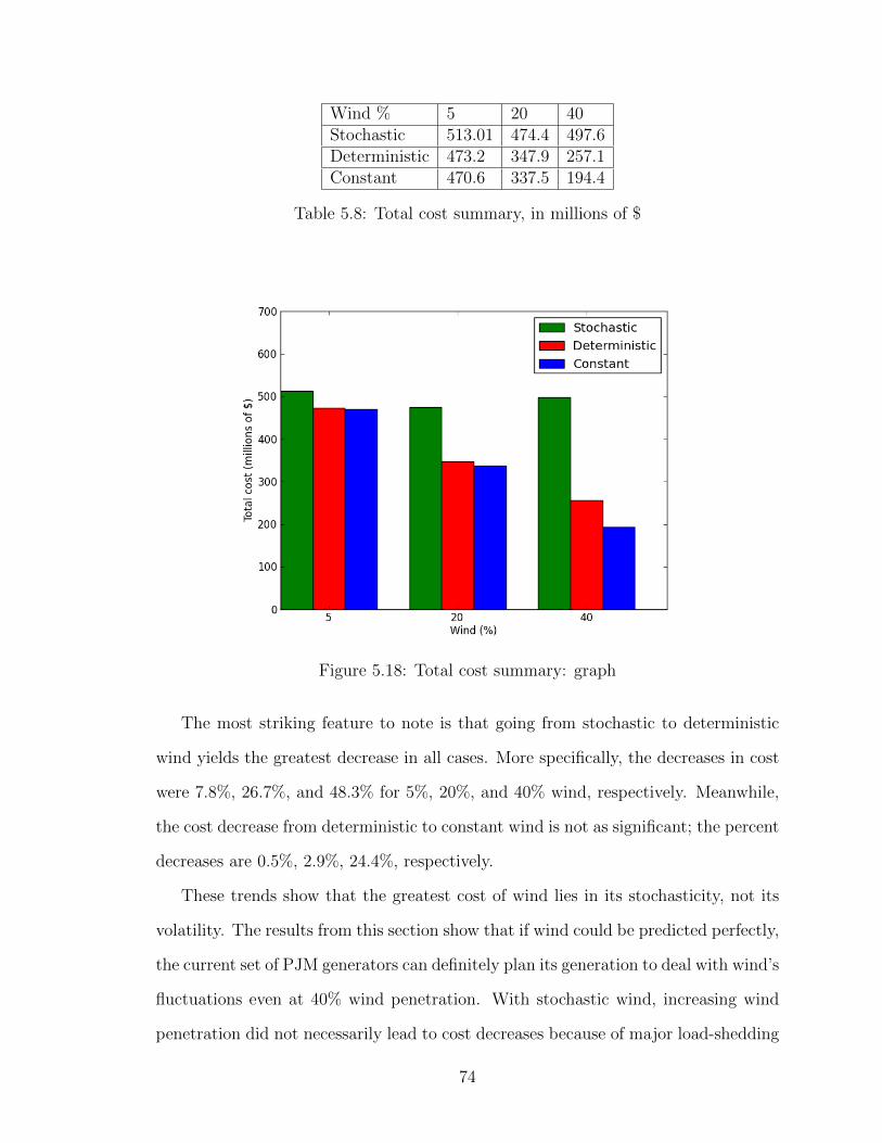
Wind % 5 20 40Stochastic 513.01 474.4 497.6Deterministic 473.2 347.9 257.1Constant 470.6 337.5 194.4
Table 5.8: Total cost summary, in millions of $
Figure 5.18: Total cost summary: graph
The most striking feature to note is that going from stochastic to deterministic
wind yields the greatest decrease in all cases. More specifically, the decreases in cost
were 7.8%, 26.7%, and 48.3% for 5%, 20%, and 40% wind, respectively. Meanwhile,
the cost decrease from deterministic to constant wind is not as significant; the percent
decreases are 0.5%, 2.9%, 24.4%, respectively.
These trends show that the greatest cost of wind lies in its stochasticity, not its
volatility. The results from this section show that if wind could be predicted perfectly,
the current set of PJM generators can definitely plan its generation to deal with wind’s
fluctuations even at 40% wind penetration. With stochastic wind, increasing wind
penetration did not necessarily lead to cost decreases because of major load-shedding
74

issues. With perfect wind predictions, however, load-shedding becomes almost a non-
issue, even though the wind output is still highly volatile.
In a way, the deterministic wind scenario explored in this section represents the
best-case results for the UC Model. Obviously, predictions will never be able to
perfectly match the actual wind, but this scenario still shows that increased wind
penetration is possible with the current set of PJM generators as long as the wind
predictions are reasonably accurate. The wind predictions used in this thesis were
less than ideal, but even then, the UC Model was able to minimize load-shedding
and generation costs with some tuning. Ultimately, better wind predictions will lead
to results that are closer to the deterministic scenario; generation costs will decrease
monotonically with increasing wind and PJM will have great economic incentive to
introduce more wind energy into its share of the grid.
75

Chapter 6
Conclusion and Further Research
Overall, simulations with the UC Model suggests that the current set of PJM gener-
ators is well-equipped to deal with 5% wind penetration with minimal load-shedding.
With 20% and 40% wind, however, the model needs to consistently under-predict
wind for the Day-Ahead Model in order to minimize costs and load-shed. This chap-
ter will investigate how the model could be modified to overcome these obstacles in
the future.
6.1. Energy Storage
Current wind predictions in the UC Model often lead to severe shortages and overages,
which ultimately inflate the total fuel costs. Having batteries, or any form of energy
storage, in the model could counteract this unfortunate result. To minimize the cost of
the battery, it will be useful to calculate the minimum capacity required to eliminate
shortages in a trial run of the simulation. Calculating this capacity would require
observing the load-shed as it evolves with time. Fortunately, the code built for this
thesis can produce such outputs, as shown in Figure 6.1.
The black horizontal line marks the baseline, where the load-shed is at 0. When-
ever the load-shed curve goes above this line, the system is incurring a shortage,
76

Figure 6.1: Load shed vs. time at 40% wind and q = 0.6
and vice versa for overage. Calculating the minimum battery capacity from this data
would require extensive research in the future, but a simple heuristic will be suggested
here as a starting point.
Denote the load-shed curve in Figure 6.1 as x(t). That is, x(t) > 0 signifies a
shortage at time t, and x(t) < 0 signifies an overage at time t. Now, let y(t) be the
total shortage incurred by the system by time t, which can be calculated recursively
as follows:
y(t) = max (0, y(t− 1) + x(t)) , where y(0) = 0
Let C be the minimum battery capacity. Assuming that the UC Model runs until
time t′, a reasonable approximation would be C = maxt
yt. Basically, this heuristic
would involve running the UC Model for t′ hours, where t′ is large, and then setting
the sample battery capacity as the maximum total shortage during the time period
[0,t′]. Repeated simulations will yield more sample battery capacities, from which
perhaps an average could be taken to reach the final estimate.
77

Obviously, this sample heuristic does not consider battery efficiency, the cost of
storage, and the other important subtleties involving energy storage. Nevertheless,
starting from the load shed vs. time perspective as shown in Figure 6.1 should serve
as a reasonable starting point for anyone wanting to do further studies on storage.
6.2. Better Wind Predictions
From a data perspective, this UC Model could be improved further by having better
wind predictions. As shown by the deterministic wind study in Section 5.3, more
accurate wind predictions will most likely lead to significant cost and load-shed de-
creases, especially at higher levels of wind penetration. Thankfully, there is still
much room for improvement in this regard. As detailed in Chapter 3, this thesis uses
a time-series method to generate wind predictions, which leaves much to be desired
in terms of accuracy.
A possible replacement for time-series wind modeling is the Weather Research and
Forecasting (WRF) model, a work-in-progress climate-based wind prediction system.
Because it is climate-based, it does not fall prey to the faults of models based on
time series, which rely far too much on short-term correlation that is inappropriate
for day-ahead forecasts. Future implementations of this UC Model could certainly
utilize other methods of wind prediction, but the basic idea of shifting to a climate-
based prediction model is highly recommended.
6.3. Final Remarks
Overall, the results of this thesis show a promising future for wind energy in the
PJM grid. At all wind penetration levels explored, the model was able to eliminate
shortages and minimize costs after some tuning. While the current results are quite
satisfactory, the model still leaves room for improvement, as discussed earlier in this
78

chapter. Future implementations of this UC Model would include battery storage, as
well as an updated system for wind predictions. With storage smoothing out wind
volatility and better wind predictions sorting out wind stochasticity, the simulated
total costs are certain to decrease from their current values. In conclusion, the re-
sults of this thesis show that with some fine-tuning, the PJM transmission grid will
certainly be ready for increased wind penetration that is to come in the future.
79
Bibliography
[1] AWC (2011). Atlantic Wind Connection Intro. Atlantic Wind Connection.
http://atlanticwindconnection.com/awc-intro
[2] AWEA (2011). 3rd quarter Public Market Report. American Wind Energy Asso-
ciation
[3] R. Barth, H. Brand, P. Meibom, and C. Weber (2006). A Stochastic Unit-
Commitment Model for the Evaluation of the Impacts of Integration of Large
Amounts of Intermittent Wind Power. International Conference on Probabilistic
Methods Applied to Power Systems, 1-8.
[4] Botterud, A., Wang, J., Monteiro, C., & Miranda, V. (2009).
Wind Power Forecasting and Electricity Market Operations (Vol.
2030, pg 1-13). San Francisco: IAEE International Conference.
http://www.usaee.org/usaee2009/submissions/OnlineProceedings/Botterud etal paper.pdf.
[5] Chandley, J.D. (2001). A standard market design for regional transmission orga-
nizations. The Electricity Journal, 14(10).
[6] Chang, G. W., Tsai, Y.D., Lai, C.Y., & Chung, J.S. (2004). A Prac-
tical Mixed Integer Linear Programming Based Approach for Unit
Commitment. Power Engineering Society General Meeting, IEEE.
http://ieeexplore.ieee.org/stamp/stamp.jsp?arnumber=01372789&tag=1.
80

[7] P. Che and L. Tang (2009). A Lagrangian Relaxation Approach for Unit Commit-
ment with Stochastic Disruption Management. International Joint Conference on
Computational Sciences and Optimization, 998-1001.
[8] Ott. A. L. (2003). Experience with PJM Market Operation, System Design, and
Implementation. IEEE Transactions on Power Systems. 18(2) 528-534.
[9] Padhy, N.P. (2004). Unit Commitment - A Bibliographical Survey. IEEE Trans-
actions on Power Systems, 19(2). 1192-1205.
[10] PJM. (2009). PJM Manual 12: Balancing Operations. ReVision. PJM.
http://www.pjm.com/ /media/documents/manuals/m12.ashx.
[11] PJM. (2010). PJM Manual 11: Scheduling Operations. ReVision. PJM.
http://www.pjm.com/ /media/documents/manuals/m11.ashx.
[12] PJM. (2010). PJM Manual 14D: Generator Operational Requirements. ReVision
http://www.pjm.com/ /media/documents/manuals/m14d.ashx.
[13] Pablo A. Ruiz, C. Russ Philbrick, Eugene Zak, Kwok W. Cheung, and Peter W.
Sauer (2009). Uncertainty Management in the Unit Commitment Problem. IEEE
Transactions on Power Systems, 24(2). 642-651. p
[14] Snyder, Brian and Mark J. Kaiser (2008). Ecological and Economic Cost-Benefit
Analysis of Offshore Wind Energy. Renewable Energy, 34(6):1567-1578.
[15] Tingfang, Y. and T.O. Ting (2008). Methodological Priority List for Unit Com-
mitment Problem. International Conference on Computer Science and Software
Engineering, 176-179.
[16] Tuohy, Aidan, Peter Meibom, Eleanor Denny, and Mark O’Malley (2009). Unit
Commitment for Systems with Significant Wind Penetration. IEEE Transactions
on Power Systems, 24(2):592-601.
81

[17] Ummels, Bart C., Madeleine Gibescu, Engbert Pelgrum, Wil L. Kling, and Arno
J. Brand (2007). Impacts of Wind Power on Thermal Generation Unit Commit-
ment and Dispatch. IEEE Transactions on Energy Conversion, 22(1):44-51.
[18] US Department of Energy. (2008). 20% Wind Energy by 2030. Wind Energy.
http://www.eia.doe.gov/emeu/aer/pdf/pages/sec1.pdf.
[19] U.S. Department of Energy. (2011). Strategies and Decision Support Systems
for Integrating Variable Energy Resources in Control Centers for Reliable Grid
Operations.
[20] Watson, S.J., Landberg, L., and Halliday, J.A. (1994). Application of wind speed
forecasting to the integration of wind energy into large scale power systems. Gen-
eration, Transmission and Distribution, IEEE Proceedings, 141(4). 357-362.
[21] Xie, T., Pejnovic, N., Lees, A.F., and Ewing E. (2008). Wind energy: A through-
out examination of economic viability. Energy and Energy Policy, University of
Chicago.
[22] Yan, J.H. and Stern, G.A. (2002). Simultaneous Optimal Auction and Unit Com-
mitment for Deregulated Electricity Markets. The Electricity Journal. 15(9). 72-
80.
[23] Zhou, Jessica (2010). 20% Generation and the Wind Market. Senior Thesis,
Princeton University.